Vol. 195: 47-59,2000 MARINE ECOLOGY PROGRESS SERIES Mar Ecol Prog Ser l Published March 31

Identification of 72 phytoplankton species by radial basis function neural network analysis

of flow cytometric data

Lynne B o d d y l l * , C . W. ~ o r r i s ~ , M. F. ~ i l k i n s ' , Luan ~l-Haddad2, G . A. ~ a r r a n ~ , R. R. Jonker4, P. H. Burkil13

'Cardiff School of Biosciences, University of Cardiff. Cardiff CFlO 3TL, United Kingdom 2 ~ c h o o l of Computing. University of Glamorgan. Pontypridd. United Kingdom

3 ~ e n t r e for Coastal and Marine Sciences, Plymouth Marine Laboratory, hospect Place, West Hoe, Plymouth PL13DH, United Kingdom 4AquaSense Lab. Kruislaan 411.1090 HC Amsterdam, The Netherlands

ABSTRACT: Radial basis function artificial neural networks (ANNs) were trained to discriminate be- tween phytoplankton species based on 7 flow cytometric parameters measured on axenic cultures. Comparison was made between the performance of networks restricted to using radially-symmetric basis functions and networks using more general arbitrarily oriented ellipso~dal basis functions, with the latter proving significantly superior in performance. ANNs trained on 62, 54 and 72 taxa identified them with respectively 77, 73 and 70% overall success. As well as high success in identification, high confidence of correct identification was also achieved. Misidentifications resulted from overlap of char- acter distributions. Improved overall identification success can be achieved by grouping together spe- cies with similar character distributions. This can be done within genera or based on groupings indi- cated in dendrograms constructed for the data on all species. When an ANN trained on 1 data set was tested with data on cells grown under different light conditions, overall successful identification was low (<20%), but when an ANN was trained on a combined data set identification success was high (>?0%). Clearly it is essential to include data on cells covering the whole spectrum of biological varia- tlon. Ways of obtaining data for training ANNs to identify phytoplankton from field samples are dis- cussed.

KEY WORDS: Radial basis functions. Neural networks . Principal component analysis . Dinoflagellates - Prymnesiomonads . Flagellates - Cryptomonads . Diatoms

INTRODUCTION

Phytoplankton play a pivotal role in marine ecosys- tems - collectively fuelling the food web, sometimes forming nuisance blooms, and being implicated in cli- mate control. Knowledge of their population dynamics, distribution and abundance in the world's oceans is crucial. There is therefore a need for a technique capa- ble of providing detailed descriptions of the species composition of phytoplankton populations from water samples. Research has been hampered by the limita- tions of traditional identification and enumeration techniques. Microscopic analysis in the laboratory is

laborious and time-consuming, abundance estimates are uncertain due to limitations on the number of cells that can be counted, and interesting phenomena can- not be followed up directly because analysis is often performed a long time after sampling. The use of image analysis is one possibility, and has been used success- fully to discriminate 23 dinoflagellate species (Culver- house et al. 1996). I t is, however, computationally in- tensive. HPLC has been used as a chemotaxonomic technique for bulk samples, but it has limited use as a diagnostic tool because it cannot provide fine resolu- tion of taxa (Jeffrey et al. 1997). It is also slow.

Analytical flow cytometry (AFC) may provide a solu- tion to this problem. Light scatter, diffraction and fluo- rescence parameters are measured on indvidual cells, at rates of up to 103 cells S-' (Burkill& Mantoura 1990), pro-

O Inter-Research 2000 Resale of full article not perrnltted

4 8 Mar Ecol Prog Ser 195: 47-59, 2000

ducing sets of characteristic 'signature' data patterns et al. 1994, Wilkins et al. 1994a,b, 1996), but, apart (1 for each cell) which may allow taxa to be discrimi- from 1 study (Boddy et al. 1994), only a few taxonomic nated. The use of a sorter module allows individual cells, categories have been discriminated. Scaling up is not a for which the data pattern satisfies selected criteria, to be trivial task. We examine the issues involved in the collected for further culture and microscopic analysis- application of a particular ANN type, the radial basis a significant advantage over the other techniques. function (RBF) network, for the discrimination of up to

AFC has already proved a valuable research tool 72 phytoplankton species. RBF ANNs have been at (Jonker et al. 1995), but its potential cannot be fully least as successful as other types in analysis of biologi- realised until appropriate ways of analysing the vast cal data (Wilkins et al. 1994b, 1996, Morgan et al. quantities of multivariate data that it generates have 1998). Moreover, they train rapidly and detect 'novel' been developed. Commonly, bivariate scatter plots of patterns, for which the identity is not known to the net- one flow cytometric parameter against another are still work (Morris & Boddy 1996). utilised (e.g. Hofstraat et al. 1991, Jonker et al. 1995), but this loses much of the information content of the signatures. Multivariate statistical methods have been RADIAL BASIS FUNCTION ARTIFICIAL NEURAL applied (e.g. Demers et al. 1992, Carr et al. 1996); NETWORKS while these can work well where the data distribution can be approximated by a simple parametric model, RBF ANNs are composed of 3 interconnected layers this is often not the case for AFC data, which are fre- of 'nodes', analogous to neurons (Fig. 1): an 'input layer' quently multimodal. Non-parametric statistical density containing 1 node per character (in this case AFC para- estimation methods such as Parzen windows and meter), a 'hidden layer', and an 'output layer' contain- k-nearest neighbours (Schalkoff 1992) can overcome ing 1 node per possible identity (in this case corre- this but are computationally intensive, posing prob- sponding to biological taxa). lems if the result of the analysis is to be used to drive a A data pattern is presented to the input layer, which real-time cell sorter module. serves merely to distribute input data to the hidden

An extremely powerful alternative is to employ arti- layer. Each hidden layer node (HLN) represents a sep- ficial neural networks (ANNs) (Fu 1994, Haykin 1994), arate basis function (a function for which the value which are both non-parametric and computationally depends solely on the distance between the input data efficient in use. ANNs were first developed to mimic pattern and a fixed point, termed the basis function the storage and analytical operations of the brain. centre). The basis function centres are collectively po- (Detailed treatment is provided by, for example, sitioned so as to represent the distribution of the data Caudill & Butler 1990, Boddy & Morris 1999 [both non- patterns throughout the data space. The distances be- mathematical], Schalkoff 1992, Hush & Horne 1993, tween the input data pattern and the basis function Haykin 1994 and Fu 1994.) They are not rule-based, centres are defined by a distance metric, which deter- but rather they 'learn' or 'train' from examples pre- mines the shape of the basis functions. The Euclidean sented to them. Essentially, there are 2 types of training - super- vised and unsupervised. With the Input Hidden Output

latter, patterns are presented to layer layer layer

the network and it forms its own + Amphidinium corlerae groupings of the data. In contrast, + Amphora coflaeformis with supervised training, which is + Aureodinium pigmentosum appropriate for identification, data ~ S C - H (forward scatter) + Chaetoceros calcitrans patterns (in this case flow cytomet- SSC-H (side scatter) nc signatures) of known identity + Chlorella salina

FLI -H (depolarised scatter) are presented to the ANN as ex- + Chroomonas salina

emplars. Once trained, any data FL2-H (orange fluorescence) + Chrysochromulina camella

pattern can be presented to the FL3-H (red fluorescence) -+ Chrysochromuiina chiron

ANN and the output analysed to FL3-A (integral red fluorescence) find the most likely identity of that FL3-W (time of flight) pattern. ANNs have been success- + Tetraselmis verrucosa fully used to analyse flow cytomet-

data Frankel et 1989' Fig. 1. Schematic of a radial basis function artificial neural network comprising an 1996, Balfoort et al. 1992, Morris et input layer with 7 nodes (1 per flow cytornetric parameter), a hidden layer and an out al. 1992, Smits et al. 1992, Boddy put layer with 1 node per taxon to be identified

Boddy et al.: Phytoplankton idenl :ification by neural network analysis 49

distance metric produces hyperspherical (radially symmetric) basis functions about the basis function centres. By independently scaling each dimension of the data, these generalise to hyperellipsoidal (non- radially-symmetric) basis functions for which the prin- cipal axes are constrained to lie along the axes of the data space. The Euclidean distance metric is a restric- ted form of the more general but significantly more computationally intensive Mahalanobis distance met- ric, which allows the hyperellipsoids to adopt any ori- entation that best fits the data distribution (Haykin 1994). The initial locations of the basis function centres may be randomly chosen, or be the result of some form of clustering algorithm, e.g. learning vector quantisa- tion (Kohonen 1990). The spatial extent of each basis function may either be constant or be determined by the data. The number of HLNs can be found automati- cally by starting with a large number of candidate HLNs and selecting from this an optimal subset, e.g. using an orthogonal least squares algorithm (Chen et al. 1991).

The response of all of the hidden layer basis func- tions is combined by the output layer to form a posteri- on estimates of the likelihood that the given input pat- tern belongs to each of the taxa known to the network (Richard & Lippmann 1991). Each output layer node corresponds to a different possible identity, and the most likely identity is found by selecting the output layer node with the highest output value. The decision boundaries formed between taxa (along which the 2 most likely taxa are equally probable) can be arbitrar- ily complex, depending on basis function locations, number and size.

METHODS

Phytoplankton cultures. Data were collected on 2 separate occasions during the course of 2 marine flow cytometry projects, giving rise to 2 independent data sets denoted A (containing 61 species, 1 of which [Emi- liania huxleyi] was present as 2 strains) and B (contaln- ing 54 species) (see Tables 1 & 2). Forty-three species were common to both data sets. Together the species cover a wide range of morphologies and sizes (approx. 1 to 45 pm) representative of natural nanophytoplank- todflagellate communities in Northern European seas. Phytoplankton cultures, obtained from the Plymouth Culture Collection (Marine Biological Association, UK) and the Alfred Wegener Institute (Bremen, Germany), were maintained at 15°C (+ 1°C) and were illuminated on a 12:12 h 1ight:dark cycle at 50 (A) or 130 (B) pm01 quanta m-2 S-'. Batch cultures were grown for several weeks before analysis in 250 m1 conical flasks (A) or in 1 1 polycarbonate bottles (NalgeneT"') (B), and were

sub-cultured every 3 to 4 d to maintain cultures in exponential growth. F/10 medium was generally used for culturing, although some cultures were grown in F/2 medium (Guillard & Ryther 1962), with or without soil extract.

Flow cytometric analysis. All cultures were analysed by flow cytometry (AFC) using a Becton Dickinson F A C S O ~ ~ ~ " flow cytometer equipped with a vertically polarized 15 mW argon ion laser emitting blue light at 488 nm and F ~ C S t a t i o n ~ " acquisition and analysis software, and using instrument settings that had previ- ously been found to allow good discrimination of the type of particle encountered in plankton analysis. Data acquisition was triggered on chlorophyll fluorescence using laboratory cultures of Micromonas pusilla (1 to 3 pm) to set the lower analysis threshold. The flow cytometer detector array consisted of 2 fluorescence photo-multiplier tubes (PMTs), 2 light scatter PMTs and a photodiode for forward light scatter. For each particle detected by the cytometer, measurements were made for cellular forward light scatter, integrated and peak chlorophyll fluorescence (>650 nm), the width of the chlorophyll fluorescence pulse or time-of-flight (a measure of particle length), peak phycoerythrin fluo- rescence (585 2 21 nm), and side scatter and depo- larised light scatter (to enhance the discrimination of coccolithophores). Each measurement of these 7 para- meters collectively forms a data pattern characterising an individual cell (or chaidaggregate of cells). Sam- ples were run for 4 min at a flow rate of l00 * 6 p1 min-', with analogue signals from the detectors being digi- tally converted and stored on computer as listmode data. Instrument drift was monitored by analysing Coulter Flowset calibration particles several times each day.

Software. The software used comprised 2 applica- tions developed during the AIMS (Automated Identifi- cation and Characterisation of Microbial Populations) project, running on a Pentium PC under Windows95. CytoWave is a flow cytometnc data visualisation pro- gram, allowing the data to be displayed on multiple 2-D dotplots, and clusters of events in the data to be defined and excluded if desired. AimsNet is a multi- variate data analysis program incorporating RBF ANNs, allowing ANNs to be trained to discriminate between selected phytoplankton species and groups of species. The 2 applications are closely integrated, allowing the user to select data within CytoWave, pass it to a trained ANN within AimsNet for neural network analysis, and display the results of the analysis superimposed on the original data.

Preprocessing cytometric data. The flow cytometry data for each selected culture was 'gated' using Cyto- Wave to remove any clusters of events originating from 'noise particles' such as inorganic particles, bacterial

Mar Ecol Prog Ser 195: 47-59, 2000

contaminants, cellular debris, etc. This was generally achieved by omitting all events with low red fluores- cence signals, since such 'noise' particles contain no photosynthetic pigments. The data for some cultures were multimodal, reflecting the presence of clumps of 2 or more cells and cells at different stages of develop- ment.

Before presentation to the network the data were lin- early rescaled. This procedure is commonly required by neural networks to ensure that equal emphasis is placed by the network on each input parameter when forming an identification; were this not done, the net- work would tend to make most use of the parameter with the largest absolute range of values, while ignor- ing the rest, even if they contained useful discrimina- tory information. In fact, the absolute signal intensities contain no information, since most flow cytometric pa- rameters are measured in arbitrary units that depend on factors such as instrument settings and the optical alignment. The distribution of the training data set was analysed, and a linear transformation calculated such that the distribution of each parameter of the training data set after transformation had a mean of 0.0 and a standard deviation of 1.0. This transformation was sub- sequently applied to all data presented to the network.

Training and testing procedures for RBF ANNs. AimsNet was used to train RBF ANNs to discriminate between the species in both d.ata sets and in a com- bined data set (see below). All networks were trained using 500 randomly selected data patterns for each species (i.e. data from 500 randomly selected individu- als of that species).

The training procedure started by defining 6 candi- date HLNs to represent each of the species. The basis function centres were positioned using Kohonen learn- ing-vector quantisation (Kohonen 1990). The spatial extents of the basis functions were determined by allo- cating each data pattern of the training data to the closest basis function centre, and calculating the covariance matrix of the cluster of patterns allocated to each basis function; the inverse of this matrix is then used in the calculation of the Mahalanobis distance for that basis function. An optimal subset of these HLNs was selected by means of the orthogonal least-squares elimination technique (Chen et al. 1991). The output layer weights were then calculated using matrix inver- sion. Finally the network performance was optimised to reduce the network output error by 10 iterations of a conj.ugate directions gradient descent learning proce- dure; similar proced.ures have been shown to signifi- cantly improve recognition performance (Wettsche- reck 8 Dietterich. 1992).

Once trained, the networks were tested using an independent set of 500 rand.0d.y selected data pat- terns for each species, and the results recorded in a

'misidentification matrix' M, the elements mi, of which indicated the proportion of test patterns for taxon i that were identified by the network as belonging to taxon j. From this misidentification matrix, 2 sets of probabili- ties were recorded for each taxon: (1) the probability of correct identification of a taxon; (2) the identification confidence of a taxon. The former is the a priori proba- bility that a randomly selected individual belonging to that taxon will be correctly identified. For taxon i this is estimated by m;,, the proportion of correctly identified test patterns from that taxon. The identification confi- dence of a taxon is the likelihood that a randomly selected individual identified as belonging to that taxon really does belong to that taxon, assuming that all taxa are a pnon equally likely to occur. For taxon i this is estimated by

where N is the number of taxa. Constructing a dendrogram. The presence of taxa

with overlapping AFC distributions inevitably reduces the identification confidence, because a proportion of identifications made by the network will be wrong. This is not a consequence of any deficiency in the net- work, but becduse the AFC data contain insufficient information to completely resolve between taxa. To im- prove the overall identification confidence (i.e. in- crease the a prior1 probability that the network's recog- nition of the pattern will be correct), at the expense of decreased specificity (i.e. the information obtained is less detailed), taxa which cannot be consistently dis- criminated from one another can be grouped together during training. These patterns would then be identi- fied with less precision than other patterns; however, a reliable indication that a cell belongs to taxon X or Y, but not specifically which of the two, is often prefer- able to an unreliable identification as, say, taxon X.

The misidentification matrix can be analysed to pro- duce a dendrogram (e.g. Fig. 2) that shows the natural order in which the taxa recognised by the network can be grouped together. This can be used as an objective way of finding the groupings of taxa that should be used to achleve a desired level of reliability.

Given 2 groups of taxa, denoted by G, and Gal we define the mutual misidentification probability (i.e. the probability that a pattern belonging to a taxon in G, will be misidentified as belonging to a taxon in G2 or vice-versa) by

where N is the total number of taxa in the combined group G, + GP, p ( i ) is the a pnon probability of a pat- tern from taxon i (if all taxa are assumed to be a pnori

Boddy et al.: Phytoplankton ~dentificat~on by neural network analysis 5 1

equally likely, this is equal to l/N), and p( j l i ) = m,, (the At the left hand end of the dendrogram, all the taxa element i, j of the misidentification matrix) is the a pri- are in separate groups (1 taxon per group). At each on probability that a pattern from taxon i will be stage, the groups which have the highest mutual misidentified as taxon j. The indices i and j are over the rnisidentification probability are merged; this reduces taxa in G, and G2 respectively. the probability that the network's recognition is wrong

. . . . . . . . Nephroselm~s pyriforrnis , . Nephroselm~s rotunda

r : : . .

Amphora coffaeforrnis . .

. . . . : : Hemiselmis brunnescens 3 . . . . . . Hemiselmrs rufescens . . . . . . . . . . Plagioselmis punctata . . . . . . . . Rhodella maculata . . . . . . . . Porphyridium pupureum . . . . . .

Cryptomonas maculata . . . . . . . . Cryptornonas calceiformis . . . . : : Cryptomonas appendiculata . . . . . .

Rhodomonas sp. . . . . . . Cryptomonas rostrella . . . . . .

Chroomonas salina . . . , . . Cryptomonas ret~culata . . . . . .

Chroomonas sp. . . . . . . Emiliania huxleyi bl l . . . .

. . ~ o ~ - o r n r n i r - & ~ ~ o & ~ N N N ~ ~ ~ N ~ ~ ; ' ~ r ; - O m m r . a m p m N r ~

p

. . . . Amphidinium carteme . . . . . . Aumodinium pigmentosum . . . . . . Chlorella salina . .

. . . . . . ~elagococcus subviridis . . . . . . I . .

Fig. 2. Dendrogram showing the order in which taxa were clustered by applying the method described in the text to the results matrix of a Mahalanobis network trained on data set A. Clustering proceeds from left to right. Initially each taxon is in a separate group. At each clustering stage, the 2 groups of taxa with the highest mutual confusion are merged, until only 1 group remains. The ordinate axis shows the percentage of misidentified data remaining at each clustering stage, while the dotted lines show the

positions corresponding to the 3 groupings referred to in Table 4 , with 40, 50 and 54 groups respectively

Gymnodinium micrum Gymnodinium veneficum . . . . Gymnodinium vitiligo . . . . . . . . Prorocentrum micans . . . . . . Scrippsiella trochoidea . . . . . . . . Dunalrella mrnuta . , . . . . Dunaliella tertlolecta ~ . . . . Dunaliella primolecta . , . . . . . . Chlamydomonas reglnae . . . . I . . . . Heterocapsa triquetra . . . . . . . . Promcentrum minimum . . . . . . P r o a n t r u m balticum . . . . 1 . . . . Gyrodinium aumolum . . . . . . Pleurochryas carterae . . . . 1 . . . . Chaetoceros calcitrans , . t

. . . Chrysochromulina chiton . . . . . Chrysochromul~na polylepis . . . . Chrysochromulina cymbium . . . . . Ochrosphaera neopolitana . . . .

_

. . . . . . . . . . , . . . . . . . . . .

Micromonas pusilla . . . . . . Tetmselmis impellucida . . . . . . Pheodactylum tricornutum : : . . Tetraselmis tetrathele . . . . . . Hemiselmrs v~rescens . T

Pseudopedinella sp . Prorocentrum nanum Phaeocystis pouchetir

Erniliania huxleyi 92 Pyramimonas gmssi~

Stichococcus bacillaris Prymnesium parvum

Ochromonas sp . Skeletonema costatum Pyrarnimonas obovata

Pavlova luthen Thalassiosira weissfloggii . . . .

Gymnodinium simpler . . . . . . . . Tetraselmrs venucosa . . . . . . . . Tetraselmis suecica . . . . . . 1~ . . Tetmselmis striata . . . . . . Chrysochromulina camella . . 1 1 . . , .

-

-

52 Mar Ecol Prog Ser 195: 47-59, 2000

Chlorophyceae

Dinophyceae

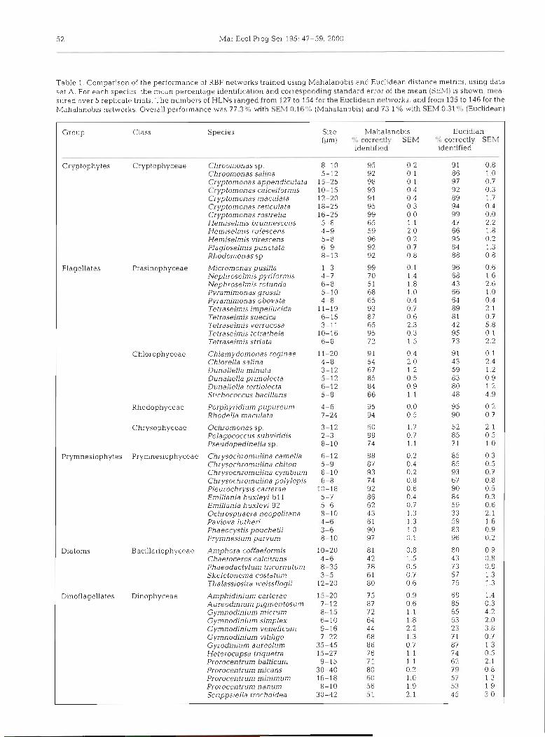
Table 1. Comparison of the performance of RBF networks trained using Mahalanobis and Euclidean distance metrics, using data set A. For each species, the medn percentage identification and corresponding standard error of the mean ( S E M ) is shown, mea- sured over 5 replicate> trials. The numbers of HLNs ranged from 127 to 154 for the Euclidean networks, and from 135 to 146 for the Mahalanobis networks. Overall performance cvas 77.3 % wth SEM 0.16"' (Mahalanobis) and 73.1 % with SEM 0.31 % (Euclidean)

Group Class Species Size Mahalanobis Eucidian (pm) % correctly S E M U/o correctly SEM

identified identified

Cryptophytes Cryptophyceae Chroomonas sp. 8-10 95 0.2 91 0.8 Chroomonas salina 5-12 92 0.1 86 1.0 Cryptomonas appendiculata 15-25 98 0.1 97 0.7 Cryptomonas calceiformis 10-15 93 0.4 92 0.3 Cryptomonas maculata 12-20 9 1 0.4 89 1.7 Cryptomonas reticulata 18-25 95 0.3 94 0.4 Cryptomonas rostrella 16-25 99 0.0 99 0.0 Hemiselmis brunnescens 5-8 65 1.1 47 2.2 Hemiselmis rufescens 4-9 59 2.0 66 1.8 Hemiselmis virescens 5-8 96 0.2 95 0.2 Plagioselmis punctata 6-9 92 0.7 84 1.3 Rhodomonas sp. 8-13 92 0.8 88 0.8

Flagellates Prasinophyceae Micromonas pusilla 1-3 99 0.1 96 0.6 Nephroselmis pyriformis 4-7 70 1.4 68 1.6 Nephroselmis rotunda 6-8 51 1.8 43 2.6 Pyramimonas grossii 5-10 68 1.0 66 1.0 Pyramimonas obovata 4-8 65 0.4 64 0.4 Tetraselm's impellucida 11-19 93 0.7 89 2.1 Tetraselmis suecica 6-15 87 0.6 8 1 0.7 Tetraselmis verrucosa 3-11 65 2.3 4 2 5.8 Tetraselmis tetrathele 10-16 95 0.3 95 0.1. Tetraselmis striata 6-8 7 2 1.5 73 2.2

Chlamydomonas reginae 11-20 9 1 0.4 91 0.1 Chlorella salina 4-8 54 2.0 43 2.4 Dunaliella minuta 3-12 67 1.2 59 1.2 Dunaliella primolecta 5-12 85 0 5 83 0.9 Dunaliella tertiolecta 6-12 84 0.9 80 1.2 Stichococcus bacillaris 5-8 66 l l 4 8 4.9

Rhodophyceae Porphyridium pupureum 4-6 95 0.0 95 0.2 Rhodella maculata 7-24 94 0.5 90 0.7

Chrysophyceae Ochromonas sp. 3-12 60 1 .? 5 2 2.1 Pelagococcus subviridis 2-3 8 8 0.7 85 0.5 Pseudopedinella sp. 8-10 7 4 1.1 7 1. 1 .O

Prymnesiophytes Prymnesiophyceae Chrysochromulina can~ella 6-12 88 0 2 85 0.3 Chrysochromulina chiton 5-9 87 0.4 85 0.5 Chrysochromulina cymbium 6-10 93 0 . 2 93 0.7 Chrysochromulina polylepis 6-8 14 0 8 6 7 0.8 Pleurochrys~s carterae 10-18 92 0.6 90 0.5 Emiliania huxleyi b l l 5-7 86 0.4 84 0.3 Emiliania huxleyi 92 5-6 62 0.7 59 0.6 Ochrosphaera neopolitana 8- 10 43 1.3 33 2.1 Pavlova lutheri 4-6 61 1.3 59 1.6 Phaeocystis pouchetii 3-6 90 1 .O 83 0.9 Prymnesiwn parvum 8-10 97 0.1 96 0.2

Diatoms Bacillariophyceae Amphora coffaeformis 10-20 8 1 0.8 80 0.9 Chaetoceros calcitrans 4-6 42 1.5 43 0.8 Phaeodactylum tricornutum 8-35 7 8 0.5 73 0.8 Skeletonema costdtum 3-5 61 0.7 57 1.3 Thalassiosira weissflogii 12-20 80 0.6 76 1.3

Dinoflagellates Amphidinium carterae 15-20 75 0.9 68 1.4 Aureodinium pigmentosum 7-12 87 0.6 85 0.3 Gymnodinium micrum 8-15 72 1.1 65 4.2 Gymnodinium simplex 6-10 64 1.8 63 2.0 Gymnodinium veneficum 9-16 44 2.2 23 3.8 Gymnodinium vitiligo 7-22 68 1.3 7 1 0.7 Gyrodinium aureolum 35-45 86 0.7 87 1.3 Heterocapsa triquetra 15-27 76 1.1 74 0.5 Prorocentrum balticum 9-15 71 1.1 62 2.1 Prorocentrum micans 30-40 80 0.3 79 0.8 Prorocentrum minimum 16-18 60 1.0 57 1.3 Prorocentrum nanum 8-10 56 1.9 53 1.9 Scrippsiella trochoidea 30-42 5 1 2.1 45 3.0

Boddy et al.. Phytoplankton identification by neural network analysis 53

Table 2. Percentage correct identification o f each species [% corr.), and the corresponding percentage confidence that identifica- tion is correct ('YO conf.) , for Mahalanobis RBF networks trained on data set A (62 taxa), data set B (54 taxa) , and the combined data set A+B ( 7 2 taxa), with 135, 132 and 147 HLNs respectively. A n asterisk indicates that one o f the networks identified the species with very d i f ferent success f rom the other networks T h e final column shows for each species i n data set B any species which it . -

was misidentified ds on more than 10% o f occasions

Group Class Species A B A+B Misidentified as species from ' % % ''c, ".. % datasetB

-- corr. conf. corr. conf. corr conf.

Cryptophytes Cryptophyreae 95 98 93 94

Flagellates Prasinophyceae

Chlorophyceae

Rhodophyceae

Chrysophyceae

Chroomonas sp. Chroomonas salina Cryptomonas appendiculata Cryptonionas cdlcciforn?is Cryptomonas maculata Cryptomonas reticulata Cryptomonas rostrella Hemiselmis brunnescens Hemiselmis rufesrens Hemi~e/lJJis virescens P1ag10svl111is punctata Rhinomonas salina Rhodomonas sp Micromonas pusilla Nephroselmis pyriformis Nephroselmis rotunda Pyramimonas grossii Pyranumonas obovatd T~traselm-s impellucida Tetrdselmis striata

Tetraselmis suecica Tetraselrnis tetrathele Tetraselmis verrucosa Chlamydomonas reginae ChloreUa salina DunaJiella miniitd Dunaliella primolerta Dunaliella tertiolecta "fannochloris atorrifi< Stichococcus barillaris Porph yr~dium pupureum Rhodella maculata Ochromonas sp Pelagococcus subviridis Pseudopedinella sp.

Prymnesiophytes Prymnesiophyceae Chrysochromulina camella Chrysochromulina chiton Chrysochromulina cymbium Chrysochromulina polylepis Chrysotila lamellosa

Diatoms

Dinoflagellates

Bacillanophyceae

Overall % correctly identified

Dicrateria inornata Emshania huxleyi Imantonia sp Ochrosphaera neopolitana Pavlova lutheri Pha~ocptis pouchetii Platychrvsis sp Pleurochrysis carterde Prymnesium parvum Amphora coffaeforrnis Chaetoceros affinis Chaetocrros calntrans Chaetoceros debilis Chaetoceros radtcans Pharoddctylum tricornutum Skeletnnema costatum Sur~relld sp Thdlawosira weissflogit Amphidinium carterde A ureodinium pigmentosum Gyn~nodinium rnicrum Gymnodinium simplex Gymnodinium vcneficun~ Cvninod~n~um vitiligo Gyrodiniiim aureolum Hpterocispua triquetra Prorocentrum balticum Proror~ntrum micans Prorocentrum minimum Prorocentruni nanum Pimocentrurn tr~estinunl Scr~ppsiella trochoidca

P punctata (14"..)

H brunnescens (17

N atomus (21 "L,)

Imantonia sp (1 l"01

E huxleyi ( l o % ) , P grossn (19".>)

T suecica (11 " c - ) , T tetrathele (14"0], T verrucosa (16'01

A. pigmentosum (15 ",,)

C, polylepis (17x1, P. poucheti (11 %)

C. chiton ( 1 1 YO), P. pouchetii (18",8b) 0, neopolitana (13 %] C rostrella (12 O;.)

C affinis (10"..l, Ochromonas sp (lo",,)

Mar Ecol Prog Ser 195: 47-59, 2000

Species Network: 1 2 3 Trained: A' B' A'+ B' Tes t ed :A1 B' A' B' A' B'

Amphidinium carterae 80 4 0 89 73 87 Amphora coffaeformis 91 77 39 85 92 81 Aureodinium pigmentosum 87 0 l 46 87 24 Chaetoceros calcitrans 90 3 0 80 89 85 Chlorella salina 57 18 0 53 47 52 Chroomonas salina 96 14 55 97 94 95 Chrysochrornulina camella 84 0 9 89 87 70 Chrysochromulina chlton 63 0 36 50 67 14 Chrysochromulina cym bium 41 0 0 91 15 88 Chrysochrornulina polylepis 63 0 1 64 70 29 Cryptornonas appendiculata 99 0 0 99 98 97 Cryptomonas calceiformis 94 9 0 96 95 94 Cryptomonas reticulata 97 0 0 98 97 94 Cryptornonas rostrella 99 1 1 93 99 87 Dunaliella min uta 79 7 9 90 80 83 Dunaliella primolecta 92 0 0 85 90 88 Emiliania h uxleyi 79 2 1 86 81 63 Gymnodinium micrum 65 0 0 59 69 60 Gymnodinium simplex 66 1 0 80 61 75 Gymnodinium vitiligo 83 0 0 60 82 39 Hemiselmis brunnescens 95 32 90 74 90 69 Hemiselmis virescens 96 62 79 93 98 94 Micrornonas pusilla 99 100 60 100 98 100 Nephroselmis pynformis 72 42 11 85 51 82 Nephroselmis rotunda 54 8 31 87 47 81 Ochromonas sp. 79 61 27 81 75 73 Ochrosphaera neopolitana 57 22 10 78 55 68 Pavlova luthen 78 0 0 94 73 95 Phaeocystis pouchetii 65 27 8 55 55 67 Plagiosehnis puncta ta 92 54 20 87 88 81 Pleurochrysis carterae 96 12 0 98 94 96 Prorocentrum micans 83 0 0 85 80 80 Prorocentrum minimum 76 0 90 94 74 89 Prorocentrum nanum 71 2 0 59 60 39 Prymnesium parvum 82 10 0 74 70 65 Pyramirnonas grossii 71 25 8 70 67 63 Pyramimonas obovata 67 8 4 42 46 37 Rhodomonas sp. 93 6 1 94 96 94 Stichococcus bacillaris 80 56 20 47 71 47 Tetraselmis stnata 75 0 0 30 74 14 Tetrasehs suecica 87 5 1 65 90 51 Tetraselmis tetrathele 95 1 0 76 94 77 Tetraselmis verrucosa 72 2 0 47 70 35

Overall % correctly identified 80 16 14 77 77 70

by the largest amount possible. As the groups are pro- each dimension) and 5 using the Mahalanobis distance gressively merged the probability that the network's metric. All initially had 6 candidate HLNs per taxon, identification is wrong falls towards zero (at the right i.e. 372 HLNs total. hand end of the dendrogram, at which point all taxa Performance with large numbers of taxa. Three net- have been merged into 1 group). works were trained and tested; one on data set A (62

Comparison of distance metrics. Ten networks were taxa), one on data set B (54 taxa) and one on the com- trained and tested on data set A, 5 using the Euclidean bined data set A+B (72 taxa). The latter data set was distance metric (allowing for independent scaling of generated by combining sets A and B together, with

data drawn equally from A and B to rep- resent species common to both data sets.

Table 3. Percentage correct identification of 3 networks trained on data set All networks used the ~ ~ h ~ l ~ ~ ~ b i ~ dis- A ' alone (131 HLNs), data set B' alone (139 HLNs) and the combined data set A ' + B ' (146 HLNsJ (43 species in each case). Each network was tested for its metric with 4, and candidate

43 species common to both data sets A and B. These new data sets were denoted A' and B' respectively. Three networks were trained: one on data set A', one on

ability to identify the species from both A' and B'

data set B ' , and one on the combined data set A'+ B' generated as above (all contain- ing 43 taxa). All 3 used the Mahalanobis distance metric, initially with 6 candidate HLNs per taxon, I.e. 258 HLNs total. All 3 networks were tested using both A' and B'.

Effect of grouping taxa on overall iden- tification success. The test results of one of the networks trained on data set A

HLNs per taxon (totals of 248, 216 and 216 HLNs) respectively.

Effect of biological variation on identi- fication accuracy. Two new data sets were created using only the data for the

were analysed and the corresponding dendrogram plotted (Fig. 2). Five further networks were trained and tested on data set A, using the following grouping schemes: grouping species within a ge- nus together if their mutual misidentifica- tion probability was greater than 5 %, giv- ing 50 taxa; grouping all species within a genus together, giving 37 taxa (genera); and grouping the species in the manner indicated by points 1, 2, and 3 on the den- drogram in Fig. 2, giving 54, 50 and 40 taxa and predicted successful identifica- tion rates of 82, 84 and 88% respectively. (For example, at point 1: Chrysochro- mulina chiton, C. polylepis, C. cymbium, Ochrosphaera neopolitana, Pseudopedi- nella sp. and Prorocentrum nanum were grouped, while Gymnodinium veneficum was grouped with G. vitiligo, Nephrosel- mis pyriformis with N. rotunda, and He- miselmis brunnescens with H. rufescens). All networks used the Mahalanobis dis- tance metric, initially with 6 candidate HLNs per taxon.

Boddy et al.. Phytoplankton identification by neural network analysis 55

RESULTS tified was similar, 80 and 77% respectively (Table 3). There were, however, large differences in success for 7

Comparison of distance metrics of the species: Aureodiniurn pigmentosum, Stichococ- cus bacillaris, Tetraselrnis striata and T, verrucosa

The variation between the 5 replicate optimized net- were considerably better identified within data set A' , works was low (Table 1). In'terms of overall successful and Chrysochron~ulina cymbiurn, Nephroselmis rotun- identification rate the networks employing the Maha- da, and Ochrosphaera neopolitana were better identi- lanobis distance metric consistently outperformed fied in data set B'. those employing the scaled Euclidean distance metric When the same networks were tested on data from by about 4 %. For individual species there was often lit- the opposite set from that on which they had been tle difference, but for Hemiselmis brunnescens, Tetra- trained, overall successful identification for both was selmis verrucosa, Chlorella salina, Stichococcus bacil- less than 20% (Table 3). Nonetheless, a few species laris, Ochrosphaera neopolitana and Gymnodinium were identified well: the network trained on A' could veneficum there was at least 10% and sometimes over identify Amphora coffaeformis (77 %) and Micromonas 20% greater success with Mahalanobis than with Eu- pusilla (100%) from B', while that trained on B' could clidean distance. identify Hemiselmis brunnescens (90 %), H. virescens

(79 %) and Prorocentrum minimum (90 %) from A'. When the network trained on the combined data set

Performance with large numbers of taxa A' + B' was tested on data from A' and B', overall suc- cessful identification was 77 and 70 % respectively.

Successful identification rate of the network trained However, a quarter of the species were still poorly on data set A (62 taxa, 135 HLNs) was 77%; that identified (<?0% success); the species poorly identi- trained on data set B (54 taxa, 132 HLNs) was 73 %; fied differed between the 2 sets (Table 3). and that trained on A+B (72 taxa, 147 HLNs) was 70% (Table 2). Nine, 15 and 23 species respectively were identified with <60% success. When percentage Effect of grouping taxa on overall correct identification was high, so too usually was identification success confidence of correct identification. Exceptions include Gymnodiniurn veneficum, with 8 1 % correct iden- Grouping together species that were misidentified as tification but only 52% confidence of correct identifi- one another improved overall percentage of correct cation, and Tetraselmis verrucosa, with 84 % success- identification (Table 4). Grouping together all species ful identification but only 63% confidence of correct in a genus resulted in an overall success similar to identification. Though many species were identified when only species within a genus were grouped if equally well or equally poorly by all of the networks they were considerably misidentified (>5%) with each in which they were included, about 18 species were other, even though the former resulted in 37 groups identified with considerably different success by one and the latter in 50 groups. Grouping according to the of the networks (Table 2) . Notable examples are: dendrogram resulted in a success similar to that pre- Gymnodinium vitiligo identified with 69 and 56% dicted by the dendrogram (compare Table 4 with success respectively by the data set A and B net- Fig. 2 ) . works, but only with 11 % success by the network trained On the data set Table 4. Effect of different groupings of species from data set A on the A+B; Aureodinium pigmentosum with performance of Mahalanobis RBF networks

86% success in the data set A network, but only 44 and 53% success respectively by the networks for data set B and for A+B.

Effect of biological variation on perfor- mance accuracy

When the networks trained on data sets A' and B' (43 taxa) were tested on the data set on which they had been trained, the overall percentage of cells correctly iden-

~ ~ t ~ ~ ~ k No. of No. of Overall HLNs groups %

correctly identified

All species separate 157 62 76 8

Species within a genus grouped together when percentage misidentified >5% 147 50 83.7

All taxa within genus grouped together 135 37 84.0

~~~d~~~~~~ grouping 1 (see ~ i ~ . 2) 154 54 83.5

Dendrogram grouping (see Fig. 2) 163 50 85.6

Dendrogram grouping (see Fig, 2, 167 40 88.7

56 Mar Ecol Prog Ser 195: 47-59,2000

DISCUSSION important. High success in identification of a species is not sufficient alone since other species may also be

This study demonstrates that previous results with a identified (incorrectly) as that species, giving an over- small (12 species) data set (Wilkins et al. 1996) can be estimate of occurrence in mixed population~. scaled to a large number of species. Identification of Species which were successfully identified by net- phytoplankton by RBF networks employing the Maha- works trained on all 3 data sets clearly have discrimi- lanobis distance metric (termed ARBF) are superior to natory flow cytometric 'fingerprints', whereas those networks using the scaled Euclidean distance, which which are consistently identified with low success do allows for the differen.t individual variances of the data not. The reasons are less clear cut as to why the suc- along each dimension but uses none of the covariance cessful identification rate of some of the species should structure. Considerably better ~dentification of some differ considerably between the 2 data sets. It is species when using the Mahalanobis distance proba- unlikely to be due to any inherent problems with the bly results from the arbitrary orientation of the Maha- ANN approach, as variation between replicates was lanobis basis function better modelling the underlying low (Table 1). Occasionally it may simply be due to dif- flow cytometry parameter distributions for these spe- ferent positioning of the decision boundaries between cies. species produced by the networks. This is certainly

Overall successful identification in excess of 70% for likely to be the case where species not common to both 72 species compares favourably with results of prelim- data sets are identified more successfully by the net- inary studies: 84 % for 12 species using ARBF (Wilkins work trained on the combined data set than by the net- et al. 1994b), 92 % for 34 species with ARBF (Wilkins et work trained only on the data set in which they al. 1999), and with 75 % for 42 strains (40 species) using occurred, e.g. Gymnodinium veneficium, Hemiselmis a multilayer perceptron (MLP or back propagation) rufescens, Platychrysis sp. and Tefraselmis verrucosa ANN (Boddy et al. 1994). The very high success in the (Table 2) . For example, in the case of Platychrysis sp., earlier study with 34 species (Wilkins et al. 1999) was which is recognised with 43% accuracy by the net- attributable to the fact that both marine and freshwater work trained on B alone but with 72 % accuracy by the species having different characteristics were used and network trained on A+B, the discrepancy is explained that 11 flow cytometric parameters were available as principally by the fact that the network trained on B opposed to the 7 used here. alone misidentifies 28% of Platychrysis sp. as Prymne-

The high confidence of correct identification ob- sium parvum (Table 2): the reason for this can be seen tained for most species identified successfully is very by examining the flow cytometric distributions (Fig. 3).

The network trained on the combined data set moves the decision boundary between the species such that only 3 % of Platychrysis sp. is misidentified as P. parvum; this how- ever means that the proportion of P. parvum identified correctly falls from 61 to 37%. Where the identification of a species by the network trained on the combined data set is

(Y worse than that by the network trained on 'd either data set alone, the discrepancy may

also be explained by species present in the other data set having overlapping character distributions.

For some species common to both data . *.- -

sets, identification rates differed substan- tially between the data sets (Tables 2 & 3).

PC1 This is almost certainly due to the same spe- cies having different flow cytometric signa-

Fig. 3. Distributions of Prymnesiurn parvum from data set A ( ) and data tures under the different light

set B (X) and Platychrysis sp. from data set B (o), projected on the plane used for data sets A and B. The low light of the first 2 pnncipal, components (PC). The distribut~ons of Platychrysis intensity for A would have resulted in a sp. and P. parvum from data set B overlap considerably. When the distri- bution for P parvum includes data from data set A (which does not sig- nificantly overlap the distribution of Platychrysissp.) the optimal decision boundary is moved and the correct identification rate for Platychrysis sp.

increases

larger quantity of photosynthetic pigments than for B, yielding higher fluorescence sig- nals. The different flow cytometric signa- tures can be seen in Aureodinium pigmento-

Boddy et al.: Phytoplankton identificatlon by neural network analysis

sum and Chrysochromulina camella, for example, by plotting the first principal component against the sec- ond (Fig. 4). With the latter, although the populations have different flow cytometric characteristics, identifi- cation success is still high in all networks, presumably because both fingerprints are different from those of other species.

When the basis f.unctions have modelled the data well (e.g with an optimized ARBF ANN), misidentifi- cations result from overlap of character distributions. To improve identification success of species whose character distributions overlap, different and/or addi- tional discriminatory characters are required. Group- ing together taxa that were misidentified as one an- other appears to be a good approach to increasing

overall successful identification. If it is necessary to dis- criminate further between species that have been grouped together, and no additional flow cytometric measurements can be obtained, the parameter values that discriminate the group from the rest of the cells in a sample can be used to trigger the flow cytometer's sorting facility. Sorted cells could then be examined using more traditional identification approaches.

The poor performance of networks in making identi- fications from data sets collected at different times and under different growth conditions highlights a major problem in using this approach for identification of natural mixed populations. Clearly, different popula- tions (i.e. a strain grown under different conditions, or different strains) of a species may have different flow

cytometric character distributions (Fig. 4 ) . So long as all of the biological variation is covered in the training data set then good identification can be achieved, as evidenced by the success when training data were selected from both data sets. The high iden- tification success for a few species can be

Fig. 4. Plots showing the distributions of (a) Aureodinium pigrnentosun~ and (b) Chrysochromulina carnella, from data set A (+) and data set B (o),

projected onto the plane of the first 2 principal components (PC)

explained by the character distributions (or at least the discriminatory set of characters) remaining similar when the cells were

6 grown under different conditions. For exam- ple, Micromonas pusilla is easily discrimi- nated because it is considerably smaller than all other species.

CONCLUSIONS

RBF ANN analysis of flow cytometric data phytoplankton populations provides a pow- erful quantitative, discriminatory tool. To produce a system capable of identifying field samples, it will be essential to cover the whole spectrum of biological variation within a species encountered in the natural envi- ronment in the training data set. It may be possible to achieve this by culturing under a range of conditions, though obtaining train- ing data from actual field samples may be a better alternative. This could be achieved, for example, by performing a statistical (Sneath & Sokal 1973, Dunn & Everitt 1982) or neural (Kohonen 1990, Wilkins et al. 1994a) cluster analysis on a natural sample and then sorting samples into clusters for microscopic identification. Once taxonomic identities can be placed on clusters, these data can form a training set for an ANN, which can subsequently be used for rapid identification of large numbers of cells.

Mar Ecol Prog Ser 195: 47-59, 2000

Research into methods for obtaining training data sets from field samples must be a high priority for the future.

A second issue to be addressed is to ensure that the trained ANNs are not tied to any individual cytometer instrument. A solution may be to use standardised cal- ibration beads to define mathematical transformations capable of reducing data captured on specific cytome- ters, at specific instrument settings, to a standard form. These transformations can then be applied to all data before presentation to the ANN. Any parameters miss- ing from the data will need to be estimated (Boddy et al. 1998).

Finally, it also remains to establish a procedure for converting the results of an ANN analysis of a mixed sample into an estimation of the relative proportions of the different species components, together with reli- able confidence limits on the proportion estimates. This work is currently ongoing.

Acknowledgements. The AimsNet and CytoWave software were developed during AIMS, a project funded by the Com- mission of the European Community, CEC grant no. MAS3- CT97-0080. Thanks to all partners for valuable discussion. Flow cytometric measurements were made as part of a Nat- ural Environment Research Council PRiME Special Topic Award (GST/02/1062) (data set A), and during the AIMS pro- ject (data set B) We also thank the Alfred Wegener Institute for provision of some cultures.

LITERATURE CITED

Balfoort HW, Snoek J , Smits JRM, Breedveld LW, Hofstraat JW, Ringelberg J (1992) Automatic identification of algae: neural network analysis of flow cytometric data. J Plank- ton Res 14:575-589

Boddy L, Morris CW (1999) Artificial neural networks for pat- tern recognition. In: Fielding AH (ed) Machine learning methods for ecological applications. Kluwer, Dordrecht, p 37-87

Boddy L, Morris CW, Wilkins MF, Tarran GA, Burkdl PH (1994) Neural network analysis of flow cytometric data for 40 marine phytoplankton species. Cytometry 15:283-293

Boddy L, Wilkins MF, Morris CW (1998) Effects of missing data on neural network identification of biological taxa: RBF network discrimination of phytoplankton from flow cytometry data. In: Dagli H, Akay M, Buczak CLP, Ersoy AL, Fernandez BR (eds) Intelligent engineering systems through artificial neural networks, Vol 8. American Soci- ety of Mechanical Engineers Press, New York, p 655-666

Burkill PH, Mantoura RFC (1990) The rapid analysis of single marine cells by flow cytometry. Philos Trans R Soc A 333. 99-112

Carr MR, Tarran GA, Burkill PH (1996) Discrimination of ma- rine phytoplankton species through the statistical analysis of their flow cytometric signatures. J Plankton Res 18: 1225-1238

Caudill M, Butler C (1990) Naturally intelligent systems. MIT Press, Cambridge, MA

Chen S, Cowan CFN, Grant PM (1991) Orthogonal least

squares learn~ng algorithm for radial basis function net- works. IEEE Trans Neural Networks 2:302-309

Culverhouse PF, Slmpson RG. Ellis R, Lindley JA. Williams R, Parisini T, Reguera B, Bravo I. Zoppoli R, Earnshaw G, McCall H, Smith G (1996) Automatic classification of field- collected dinoflagellates by artificial neural network. Mar Ecol Prog Ser 139:281-287

Demers S, Im J , Legendre P, Legendre L (1992) Analysing multivariate flow cytometrlc data in aquatic sciences. Cy- tometry 13:291-298

Dunn G, Everitt BS (1982) An introduction to mathematical taxonomy. Cambridge University Press, Cambridge

Frankel DS, Olson RJ, Frankel SL, Chisholm SW (1989) Use of a neural net computer system for analysls of flow cyto- metric data of phytoplankton populations Cytometry 10. 540-550

Frankel DS, Frankel SL, Binder BJ, Vogt RF (1996) Applica- tion of neural networks to flow cytometry data analysis and real-time cell classification. Cytometry 23~290-302

Fu LM (1994) Neural networks in computer ~ntelligence. McGraw-Hill, New York

Guillard RRL, Ryther JH (1962) Studies on marine planktonic diatoms. I. Cyclotella nand (Hustedt) and Detonula confer- vacae (Cleve) Gran. Can J Microbiol8:229-239

Haykin S (1994) Neural networks: a comprehensive founda- tion. Maxwell Macmillan International, New York

Hofstraat JW, de Vreeze IMEJ, van Zeijl WJM, Peperzak L, Peeters JCH, Balfoort HW (1991) Flow cytometric discrim- ination of phytoplankton classes by fluorescence emission and excitation properties. J Fluoresc 1:249-265

Hush DR, Horne BG (1993) Progress in supervised neural net- works - what's new since Lippmann? IEEE Sig Proc Mag 10:8-39

Jeffrey SW, Mantoura RFC, Wright SW (eds) (1997) Phyto- plankton p~gments in oceanography: guidelines to mod- ern methods. UNESCO, Paris

Jonker RR, Meulemans JT, Dubelaar GBJ, Wilkins MF, Ringelberg J (1995) Flow cytometry: a powerful tool in analysis of biomass distributions in phytoplankton. Water Sci Technol32:177-182

Kohonen T (1990) The self-organising map. Proc IEEE 78. 1464-1480

Morgan A, Boddy L, Morris CW, Mordue JEM (1998) Identifi- cation of species in the genus Pestalotiopsis from spore morphometric data: a comparison of some neural and non- neural methods. Mycol Res 102:975-984

Morris CW, Boddy L (1996) Classification as unknown by RBF networks: discriminating phytoplankton taxa from flow cytometry data. In: Dagli CH, Akay M, Chen CLP, Fernan- dez BR. Ghosh J (eds) Intelligent engineering systems through artificial neural networks, Vol 6. American Soci- ety of Mechanical Engineers Press, New York, p 629-634

Morris CW, Boddy L , Allman R (1992) Identification of basld- iomycete spores by neural network analysis of flow cytom- etry data. Mycol Res 96:697-701

Richard MD, Lippmann RP (1991) Neural network classifiers estimate Bayesian a posteriori probabilities. Neural Comp 3:461-483

Schalkoff RJ (1992) Pattern recognition: statlstlcal, structural and neural approaches Wiley International, Chichester

Smits JRM, Breedveld LW. Derksen MWJ, Kateman G, Bal- foort HW, Snoek J , Hofstraat JW (1992) Pattern classifica- tion with artificial neural networks: classification of algae. based upon flow cytometer data. Anal Chun Acta 258: 11-25

Sneath PHA, Sokal RR (1973) Numerical taxonomy. WH Free- man, San Francisco

Boddy et a1 Phytoplankton identification by neural network analysis 59

Wettschereck D, Diettench T (1992) Improving the perfor- mance of radial basis function networks by learning center locations. Adv Neural Info Process Syst 4:1133-1140

Wilkins MF, Boddy L, Morris CW, Jonker R (1996) A compar- ison of some neural and non-neural methods for identifica- tion of phytoplankton from flow cytometry data. CABIOS 12:9-18

Wilkins MF, Boddy L, Morns CW (1994a) Kohonen maps and learning vector quantization neural networks for analysis

Editorial responsibility: Otto f i n n e (Ed~tor), Oldendorf/Luhe, Germany

of multivariate biological data. Binary 6~64-72 Wilkins MF, Morris CW, Boddy L (1994b) A comparison of

radial basis function and backpropagation neural net- works for identification of marine phytoplankton from multivariate flow cytometry data. CABIOS 10:285-294

Wilkins MF, Boddy L, Morris CW, Jonker R 11999) Identifica- tion of phytoplankton from flow cytometry datd using radial basis function neural networks. Appl Environ hdicrobiol 65:4404-44 10

Subm~tted. June 22, 1999; Accepted: October 26, 1999 Proofs received from author(s): March 17, 2000