7.1 { Improper Riemann Integrals - Bucks County Community College

7The Laplace Transform

7.1 – Improper Riemann Integrals

In this section we undertake a study of improper integrals. Simply put, an improperRiemann integral is any sort of “integral” that does not conform to the definition of aRiemann integral, which requires an interval of integration [a, b] that is closed and bounded,and also a bounded real-valued function f that is defined at every point in the interval ofintegration so that [a, b] ⊆ Dom(f). If f : [0, 2]→ R is given by

f(x) =

{x3, if 0 ≤ x < 2

10, if x = 2

then the integral∫ 2

0f is a completely “proper” Riemann integral which can be evaluated using

the definition, even though f has a discontinuity at 2. This is therefore not the kind of integralwe’re concerned about at present.

Given a closed, bounded interval [a, b], the symbol R[a, b] denotes the set of all functionsthat are Riemann integrable on [a, b]. Suppose f ∈ [a, t] for all t ≥ a; that is, f is a functionthat is integrable on [a, t] for all t ∈ R such that t ≥ a. This means that∫ t

a

f ∈ R

for each t ≥ a. This observation leads us to ask whether∫ taf tends to some limiting value

L ∈ R as t→∞; that is, does the limit

limx→∞

∫ t

a

f

exist in R? Such a question arises frequently in applications, and so motivates the followingdefinition.

Definition 7.1. If f ∈ R[a, b] for all b ≥ a, then we define∫ ∞a

f = limb→∞

∫ b

a

f

and say that∫∞af converges to L if

∫∞af = L for some L ∈ R. Otherwise we say that

∫∞af

diverges.

2

If f ∈ R[a, b] for all a ≤ b, then we define∫ b

−∞f = lim

a→−∞

∫ b

a

f

and say that∫ b−∞ f converges to L if

∫ b−∞ f = L for some L ∈ R. Otherwise we say that∫ b

−∞ f diverges.

If an improper integral converges to some real number L then it is customary to say simplythat the integral “converges” or is “convergent.” An integral that “diverges” is also said tobe “divergent.” Any integral, such as those defined above, that has an unbounded interval ofintegration is called an improper integrals of the first kind.

Example 7.2. Determine whether ∫ ∞1

ln(x)

x2dx

converges or diverges. Evaluate if convergent.

Solution. It will be easier to first determine the indefinite integral∫ln(x)

x2dx.

We start with a substitution: let w = ln(x), so that dw = (1/x)dx and ew = eln(x) = x; now,∫ln(x)

x2dx =

∫we−w dw.

Next, we employ integration by parts, letting u′(w) = e−w and v(w) = w to obtain∫we−w dw = −we−w +

∫e−w dw = −we−w − e−w + C.

Hence, ∫ln(x)

x2dx = − ln(x) · 1

x− 1

x+ C = − ln(x) + 1

x+ C.

Now we turn to the improper integral,∫ ∞1

ln(x)

x2dx = lim

b→∞

∫ b

1

ln(x)

x2dx = lim

b→∞

[− ln(x) + 1

x

]b1

= limb→∞

[− ln(b) + 1

b+

ln(1) + 1

1

]= lim

b→∞

(b− ln(b) + 1

b

)= lim

b→∞

(1− 1/b

1

)= 1,

using L’Hopital’s Rule for the penultimate equality.Therefore the improper integral is convergent, and its value is 1. �

3

Given an improper integral such as∫∞af , if f(x) ≥ 0 for all x ∈ [a,∞), then the value of

the integral can be naturally interpreted as being the area under the curve y = f(x) for x ≥ a.If the integral is divergent (in this case it will equal∞), then the area is said to be infinite; andif the integral is convergent, then the area is set equal to the real number the integral convergesto. Thus the area under the curve y = ln(x)/x2, illustrated in Figure 1, is considered to be 1.Thus, the shaded region has an infinite “perimeter” and yet a finite area!

Proposition 7.3. Suppose that f ∈ R[s, t] for all −∞ < s < t < ∞. If∫ c−∞ f and

∫∞cf

converge for some c ∈ R, then for any c 6= c the integrals∫ c−∞ f and

∫∞cf also converge, and∫ c

−∞f +

∫ ∞c

f =

∫ c

−∞f +

∫ ∞c

f

Proof. Suppose∫ c−∞ f and

∫∞cf converge for some c ∈ R, meaning the limits

lima→−∞

∫ c

a

f and limb→∞

∫ b

c

f

both exist. Let c < c.For all b > c we have ∫ b

c

f =

∫ c

c

f +

∫ b

c

f,

where∫ ccf,∫ bcf ∈ R since f is integrable on [c, c] and [c, b], and so∫ ∞

c

f = limb→∞

∫ b

c

f = limb→∞

(∫ c

c

f +

∫ b

c

f

)=

∫ c

c

f + limb→∞

∫ b

c

f =

∫ c

c

f +

∫ ∞c

f. (1)

Observing that∫ ccf,∫∞cf ∈ R, we readily conclude that

∫∞cf ∈ R and hence

∫∞cf converges.

For all a < c we have ∫ c

a

f =

∫ c

a

f −∫ c

c

f,

where∫ caf,∫ ccf ∈ R since f is integrable on [a, c] and [c, c], and so∫ c

−∞f = lim

a→−∞

∫ c

a

f = lima→−∞

(∫ c

a

f −∫ c

c

f

)= lim

a→−∞

∫ c

a

f −∫ c

c

f =

∫ c

−∞f −

∫ c

c

f. (2)

Observing that∫ c−∞ f,

∫ ccf ∈ R, we readily conclude that

∫ c−∞ f ∈ R and hence

∫ c−∞ f converges.

x

y

1

0.1

0.2 Area =∫∞1

ln(x)/x2 dx = 1

Figure 1. The area under the curve y = ln(x)/x2.

4

Finally, combining (1) and (2), we obtain∫ c

−∞f +

∫ ∞c

f =

(∫ c

−∞f −

∫ c

c

f

)+

(∫ c

c

f +

∫ ∞c

f

)=

∫ c

−∞f +

∫ ∞c

f,

as desired. �

Due to Proposition 7.3 we can unambiguously define an improper integral of the first kindwhose interval of integration is (−∞,∞).

Definition 7.4. Suppose that f ∈ R[a, b] for all −∞ < a < b < ∞. If∫ c−∞ f and

∫∞cf both

converge for some −∞ < c <∞, then we define∫ ∞−∞

f =

∫ c

−∞f +

∫ ∞c

f.

and say that∫∞−∞ f converges. Otherwise we say

∫∞−∞ f diverges.

It should be stressed that∫∞−∞ f can not be reliably evaluated simply by computing the

limit

limb→∞

∫ b

−bf,

as the next example illustrates.

Example 7.5. Show that ∫ ∞−∞

2x

1 + x2dx

diverges, and yet

limb→∞

∫ b

−b

2x

1 + x2dx = 0.

Solution. Letting u = 1 + x2 gives du = 2x dx. Then∫ b

0

2x

1 + x2dx =

∫ 1+b2

1

1

udu =

[ln |u|

]1+b21

= ln(1 + b2)− ln(1) = ln(1 + b2),

and so ∫ ∞0

2x

1 + x2dx = lim

b→∞

∫ b

0

2x

1 + x2dx = lim

b→∞ln(1 + b2) =∞.

Thus ∫ ∞0

2x

1 + x2dx

diverges, and therefore ∫ ∞−∞

2x

1 + x2dx

diverges as well.On the other hand, again employing the substitution u = 1 + x2 we find that∫ b

−b

2x

1 + x2dx =

∫ 1+b2

1+b2

1

udu = 0,

5

and so

limb→∞

∫ b

−b

2x

1 + x2dx = lim

b→∞(0) = 0.

�

An improper integral of the second kind is an integral of the form∫ b

a

f,

where −∞ < a < b < ∞, for which there exists some p ∈ [a, b] such that p /∈ Dom(f). Thefollowing definition establishes how such an integral is to be evaluated, if it can be evaluatedat all, in the case when p = a or p = b.

Definition 7.6. If f ∈ R[c, b] for all c ∈ (a, b] and a /∈ Dom(f), then we define∫ b

a

f = limc→a+

∫ b

c

f

and say that∫ baf converges to L if

∫ baf = L for some L ∈ R. Otherwise we say that

∫ baf

diverges.If f ∈ R[a, c] for all c ∈ [a, b) and b /∈ Dom(f), then we define∫ b

a

f = limc→b−

∫ c

a

f

and say that∫ baf converges to L if

∫ baf = L for some L ∈ R. Otherwise we say that

∫ baf

diverges.

Very often if f is continuous on, say, (a, b] and a /∈ Dom(f), then f has a vertical asymptoteat a; that is, limx→a+ f(x) = ±∞. However, it could just be that a value for f is simply notspecified at a by construction. For example for the function

ϕ(x) =

{3x2, if x < 5

4− 8x, if x > 5

it’s seen that ϕ(5) is left undefined, and so the integral∫ 9

5ϕ is an improper integral of the

second kind. By Definition 7.6 we obtain∫ 9

5

ϕ = limc→5+

∫ 9

c

(4− 8x) dx = limc→5+

[4x− 4x2

]9c

= limc→5+

[(4(9)− 4(9)2

)−(4c− 4c2

)]=(4(9)− 4(9)2

)−(4(5)− 4(5)2

)= −208,

which shows that∫ 9

5ϕ is convergent.

Example 7.7. Determine whether ∫ 0

−1

1

x2dx


6

Solution. The function f(x) = 1/x2 being integrated has a vertical asymptote at x = 0, whichis the right endpoint of the interval of integration [−1, 0]. By Definition 7.6 we obtain∫ 0

−1

1

x2dx = lim

c→0−

∫ c

−1

1

x2dx = lim

c→0−

[−1

x

]c−1

= limc→0−

(−1

c− 1

)=∞,

which shows that the improper integral is divergent. �


0

x√4− x2

dx


Solution. Here x/√

4− x2 has a vertical asymptote at x = 2, the right endpoint of the intervalof integration [0, 2]. By Definition 7.6∫ 2

0

x√4− x2

dx = limc→2−

∫ c

0

x√4− x2

dx,

and so, letting u = 4− x2 so that x dx = −12du, we obtain

limc→2−

∫ c

0

x√4− x2

dx = limc→2−

∫ 4−c2

4

−1/2√udu = lim

c→2−

(−1

2

[2√u]4−c24

)= lim

c→2−

(2−√

4− c2)

= 2−√

4− 22 = 2.

Hence the improper integral is convergent, and its value is 2. �

The next definition addresses the circumstance when a function f is not defined at somepoint p in the interior of an interval of integration. Again, this is commonly due to f having avertical asymptote at p, so that

limx→p+

|f(x)| =∞ or limx→p−

|f(x)| =∞,

but other scenarios are possible.

Definition 7.9. Suppose that f ∈ R[a, c] for all c ∈ [a, p), f ∈ R[c, b] for all c ∈ (p, b], and

p /∈ Dom(f). If∫ paf and

∫ bpf both converge, then we define∫ b

a

f =

∫ p

a

f +

∫ b

p

f.

and say that∫ baf converges. Otherwise we say

∫ baf diverges.


−2

1

x4dx


7

Solution. Here 1/x4 has a vertical asymptote at x = 0, an interior point of the interval ofintegration [−2, 3]. Now, by Definition 7.6∫ 3

0

1

x4dx = lim

c→0+

∫ 3

c

1

x4dx = lim

c→0+

[− 1

x3

]3c

= limc→0+

(− 1

27+

1

c3

)=∞,

which shows that∫ 3

0x−4 dx is divergent. Thus, since∫ 3

0

x−4 dx and

∫ 0

−2x−4 dx

cannot both be convergent, by Definition 7.9 it’s concluded that∫ 3

−2 x−4 dx is divergent. �

The integral treated in Example 7.10, like all improper integrals of the second kind, doesnot look improper at first glance. If one is careless and undertakes to evaluate the integralby conventional means, one is likely to arrive at a reasonable-looking answer without eversuspecting that something is amiss:∫ 3

−2

1

x4dx =

[− 1

x3

]3−2

= − 1

27+

1

−8= − 35

216,

which is incorrect! So, before attempting to evaluate a definite integral, it is necessary to checkthat the integral is not improper in some way.

It is possible to have an integral that is improper in more than one sense, such as∫ ∞0

1

x2dx.

Here we have an integral of f over an unbounded interval [0,∞), so it’s an improper integralof the first kind, and also f is undefined at 0, so it’s an improper integral of the second kind.Such an integral is called a mixed improper integral.

Definition 7.11. If f ∈ R[s, t] for all a < s < t < ∞, a /∈ Dom(f), and∫ caf and

∫∞cf both

converge for some c ∈ (a,∞), then we define∫ ∞a

f =

∫ c

a

f +

∫ ∞c

f

and say∫∞af converges. Otherwise we say

∫∞af diverges.

If f ∈ R[s, t] for all −∞ < s < t < b, b /∈ Dom(f), and∫ c−∞ f and

∫ bcf both converge for

some c ∈ (−∞, b), then we define ∫ b

−∞f =

∫ c

−∞f +

∫ b

c

f

and say∫ b−∞ f converges. Otherwise we say

∫ b−∞ f diverges.

Example 7.12. Determine whether the mixed improper integral∫ ∞0

1√x(1 + x)

dx


8

Solution. We start by determining the indefinite integral∫1√

x(1 + x)dx.

Let u =√x, so that 1 + u2 = 1 + x and we replace dx with 2u du to obtain∫

1√x(1 + x)

dx =

∫2u

u(u2 + 1)du = 2

∫1

u2 + 1du

= 2 arctan(u) + c = 2 arctan(√x ) + c.

Now, ∫ 1

0

1√x(1 + x)

dx = lima→0+

∫ 1

a

1√x(1 + x)

dx = lima→0+

[2 arctan(

√x )]1a

= lima→0+

2[arctan(1)− arctan(a)]= 2[arctan(1)− arctan(0)]

= 2(π

4− 0)

=π

2,

and ∫ ∞1

1√x(1 + x)

dx = limb→∞

∫ b

1

1√x(1 + x)

dx = limb→∞

[2 arctan(

√x )]b1

= limb→∞

2[arctan(

√b )− arctan(1)

]= 2(π

2− π

4

)=π

2.

Since ∫ 1

0

1√x(1 + x)

dx and

∫ ∞1

1√x(1 + x)

dx

both converge, we conclude that∫ ∞0

1√x(1 + x)

dx =

∫ 1

0

1√x(1 + x)

dx+

∫ ∞1

1√x(1 + x)

dx =π

2+π

2= π

by Definition 7.11. �

We conclude this section with one more result concerning improper integrals called theComparison Test for Integrals, which will be needed in §7.2.

Theorem 7.13 (Comparison Test for Integrals). Suppose f ∈ R[a, x] for all x ≥ a, and0 ≤ f ≤ g on [a,∞). If

∫∞ag is convergent, then

∫∞af is convergent.

9

7.2 – Definition of the Laplace Transform

The Laplace transform is a function L whose domain consists of functions of a particularkind, and whose range also consists of functions. If f ∈ Dom(L) and F is the function that Lreturns as “output” when given f as “input,” we write L[f ] = F .1 If f is a function of t andF is a function of s, then we may also write L[f(t)] = F (s), which is taken to mean the samething since all we are doing is replacing the name of a function by its defining rule. Since L[f ]is a function of s it makes sense to write L[f ](s), which is usually done in situations when asymbol for the Laplace transform of f (such as F ) has not been given.

Definition 7.14. Given a function f : [0,∞) → R, the Laplace transform of f is thefunction L[f ] given by

L[f ](s) =

∫ ∞0

e−stf(t) dt (3)

for all s ∈ R for which the integral converges.

As the definition implies, the domain of L[f ] is the set of all s ∈ R such that the improperintegral in (3) exists as a real number. Recall that∫ ∞

0

e−stf(t) dt = limb→∞

∫ b

0

e−stf(t) dt,

so any question concerning whether the improper integral exists boils down to a question aboutwhether the associated limit of Riemann integrals exists.

Example 7.15. Find L[t2], the Laplace transform of the function t 7→ t2.

Solution. To “find” L[t2] means to find an expression for L[t2](s). By definition we have

L[t2](s) =

∫ ∞0

e−stt2 dt = limb→∞

∫ b

0

t2e−st dt. (4)

To evaluate the definite integral we employ integration by parts. Letting u(t) = t2 and v′(t) =e−st, we obtain u′(t) = 2t and v(t) = −e−st/s, and so∫ b

0

t2e−st dt =

[−1

st2e−st

]b0

−∫ b

0

−2

ste−st dt = −1

sb2e−sb +

2

s

∫ b

0

te−st dt. (5)

Now, the integral∫ b0te−st dt itself requires integration by parts. Letting u(t) = t and v′(t) =

e−st, we obtain u′(t) = 1 and v(t) = −e−st/s, and so∫ b

0

te−st dt =

[−1

ste−st

]b0

−∫ b

0

−1

se−st dt = −1

sbe−sb − 1

s2[e−st

]b0

= −1

sbe−sb − 1

s2(e−sb − 1). (6)

1Some authors use braces where we have brackets and write L{f} = F , but it is at odds with conventionaloperator notation.

10

Putting (6) into (5) gives∫ b

0

t2e−st dt = −1

sb2e−sb +

2

s

[−1

sbe−sb − 1

s2(e−sb − 1)

]=

2

s3− s2b2 + 2sb+ 2

s3esb,

and putting this result into (4) yields

L[t2](s) = lim

b→∞

(2

s3− s2b2 + 2sb+ 2

s3esb

).

This limit does not exist if s ≤ 0; however if s > 0, then by two successive applications ofL’Hopital’s Rule we obtain

limb→∞

s2b2 + 2sb+ 2

s3esb= lim

b→∞

2s2b+ 2s

s4esb= lim

b→∞

2s2

s5esb= lim

b→∞

2

s3esb= 0,

and therefore

L[t2](s) = lim

b→∞

2

s3− lim

b→∞

s2b2 + 2sb+ 2

s3esb=

2

s3

for all s > 0. �

One key feature of the Laplace transform is that when it is applied to a piecewise-definedfunction of t, the result is a function of s that is defined by a single expression.

Example 7.16. Find the Laplace transform of the function

f(t) =

1− t, if 0 ≤ t ≤ 1

0, if 1 < t ≤ 3

e2t, if 3 < t <∞

Solution. Using the usual properties of the Riemann integral established in calculus and as-suming s 6= 2, we obtain

L[f ](s) = limT→∞

∫ T

0

e−stf(t)dt

= limT→∞

(∫ 1

0

e−st(1− t)dt+

∫ 3

1

e−st · 0dt+

∫ T

3

e−ste2tdt

)= lim

T→∞

(∫ 1

0

e−stdt−∫ 1

0

te−st dt+

∫ T

3

e(2−s)tdt

)= lim

T→∞

[−1

s(e−s − 1)−

(−1

se−s − 1

s2(e−s − 1)

)+

1

2− s

(e(2−s)T − e3(2−s)

)]= lim

T→∞

[e−s + s− 1

s2+

1

2− s

(e(2−s)T − e3(2−s)

)](7)

The limit does not exist if s < 2, since we would find that e(2−s)T → ∞ as T → ∞. If s = 2the limit again does not exist, since in this case∫ T

3

e−ste2tdt =

∫ T

3

e−2te2tdt =

∫ T

3

dt = T − 3,

11

where T − 3→∞ as T →∞. However if s > 2, then e(2−s)T → 0 as T →∞, and from (7) weobtain

L[f ](s) =e−s + s− 1

s2+

1

2− s[0− e3(2−s)

]=e−s + s− 1

s2+e6−3s

s− 2,

which can be seen to be not piecewise-defined! �

The next proposition establishes that the Laplace transform is a linear transformation, alsoknown as a linear operator.

Proposition 7.17. Let f, g : [0,∞)→ R be functions such that L[f ](s) and L[g](s) are definedfor all s > α, and let c ∈ R. Then on (α,∞)

1. L[f + g] = L[f ] + L[g]2. L[cf ] = cL[f ]

Proof.Proof of Part (1). Let s > α. Then L[f ](s) and L[g](s) are both defined, which is to say thatthe limits

limT→∞

∫ T

0

e−stf(t)dt and limT→∞

∫ T

0

e−stg(t)dt

both exist. This fact allows us to use a limit law to write

L[f ](s) + L[g](s) = limT→∞

∫ T

0

e−stf(t)dt+ limT→∞

∫ T

0

e−stg(t)dt

= limT→∞

[∫ T

0

e−stf(t)dt+

∫ T

0

e−stg(t)dt

],

and thus by an established property of the Riemann integral we obtain

L[f ](s) + L[g](s) = limT→∞

[∫ T

0

(e−stf(t)dt+ e−stg(t)

)dt

]=

∫ T

0

e−st(f + g)(t)dt = L[f + g](s),

where of course (f + g)(t) = f(t) + g(t) by definition. Hence

(L[f ] + L[g])(s) = L[f ](s) + L[g](s) = L[f + g](s)

for all s > α, which proves part (1).

Proof of Part (2). Done similarly, and so left as an exercise. �

Table 7.1 gives the Laplace transforms for many frequently encountered functions. (A morecomprehensive table can be found at the end of the chapter.) Indeed the table, together withProposition 7.17, allows for easy computation of the transforms of most functions that arisein applications. To find the transform of sin bt or cos bt, let a = 0 in eat sin bt or eat cos bt,respectively. For the transform of t2, let a = 0 and n = 2 in eattn to obtain

L[t2](s) =

2!

(s− 0)2+1=

2

s3

12

f(t) L[f ](s) Dom(L[f ])

t sin bt2bs

(s2 + b2)2s > 0

t cos bts2 − b2

(s2 + b2)2s > 0

eat sin btb

(s− a)2 + b2s > a

eat cos bts− a

(s− a)2 + b2s > a

eattn, n = 0, 1, . . .n!

(s− a)n+1s > a

t−1/2√π√s

s > 0

tn−1/2, n = 1, 2, . . .1 · 3 · 5 · · · (2n− 1)

√π

2nsn+1/2s > 0

Table 1. Laplace transforms of common functions.

as found in Example 7.15. For the transform of 1, let a = 0 and n = 0 in eattn to obtain

L[1](s) =0!

(s− 0)0+1=

1

s

from the table.

Example 7.18. Find L[f ] for f(t) = e−5t sin πt− cosh 8t+ 7.

Solution. Recall that the hyperbolic cosine function cosh is defined by cosh(x) = 12(ex + e−x).

By Proposition 7.17 we obtain

L[f ](s) = L[e−5t sin πt− cosh 8t+ 7

](s)

= L[e−5t sin πt

](s)− L[cosh 8t](s) + L[7](s)

= L[e−5t sin πt

](s)− L

[12e8t + 1

2e−8t

](s) + L[7](s)

= L[e−5t sin πt

](s)− 1

2L[e8t](s)− 1

2L[e−8t

](s) + 7L[1](s) (8)

Now we use Table 7.1 to get

L[e−5t sin πt

](s) =

π

(s+ 5)2 + π2

13

for s > π,

L[e8t](s) =

1

s− 8for s > 8,

L[e−8t

](s) =

1

s+ 8for s > −8, and finally L[1](s) = 1/s for s > 0. Putting all these results into (8) gives

L[f ](s) =π

(s+ 5)2 + π2− 1

2· 1

s− 8− 1

2· 1

s+ 8+ 7 · 1

s

=π

(s+ 5)2 + π2− s

s2 − 64+

7

s

for s > 8, which is the intersection of the domains of the individual transforms. �

Not all functions have a Laplace transform. The remainder of this section will be devotedto developing some results that will help determine whether or not a given function has atransform.

Definition 7.19. Let −∞ < a < b <∞. A function f is piecewise continuous on [a, b] ifit satisfies the following:

1. f is continuous on [a, b] except at a finite number of points, at most.2. At each c ∈ (a, b) where f is discontinuous the limits limt→c+ f(t) and limt→c− f(t) both exist

in R.3. If f is discontinuous at a, then limt→a+ f(t) ∈ R; and if f is discontinuous at b, then

limt→b− f(t) ∈ R.

A function f is piecewise continuous on [a,∞) if it is piecewise continuous on [a, c] forall c > a.

A careful reading of Definition 7.19 should make it clear that in order for f to be piecewisecontinuous on [a, b] or [a,∞), it is not required that f(t) be defined for all t in [a, b] or [a,∞),respectively. This is because a function is considered to be discontinuous at any point outsideits domain. Thus, for example,

f(t) =

{3t2, if t < 5

4− 8t, if t > 5

is piecewise continuous on [0, 10] and [0,∞), with f considered discontinuous at 5 since thedomain of f is (−∞, 5) ∪ (5,∞). As another example, g(t) = 1/t is not piecewise continuouson [−1, 1] since

limt→0+

1

t=∞ /∈ R,

which runs afoul of part (2) of Definition 7.19.It is a fact, easily verifiable, that a piecewise continuous function defined on a closed,

bounded interval is necessarily a bounded function.

Remark. For our own purposes we will only work with piecewise continuous functions thatare defined at every point on a closed interval of the form [a, b] or [a,∞).

14

To prove the following proposition we need to recall two facts from calculus: first, iff ∈ R[a, b] and g = f on [a, b] except at a finite number of points, then g ∈ R[a, b] with∫ bag =

∫ baf ; and second, if f ∈ R[a, c] and f ∈ R[c, b] (where a < c < b), then f ∈ R[a, b]. The

latter fact is easily extended: if

f ∈ R[t0, t1],R[t1, t2], . . . ,R[tn−1, tn],

for t0, t1, . . . , tn ∈ R such that t0 < t1 < · · · < tn, then f ∈ R[t0, tn].

Proposition 7.20. If f : [a, b]→ R is piecewise continuous, then f ∈ R[a, b].

Proof. Suppose that f : [a, b] → R is piecewise continuous. If f is continuous on [a, b] thenf ∈ R[a, b] follows immediately since continuity on a closed, bounded interval implies integra-bility. Suppose that f has precisely n discontinuities on [a, b] for some n ∈ N. Thus f hasdiscontinuities at points t1, . . . , tn ∈ [a, b], where a ≤ t1 < · · · < tn ≤ b. For convenience wewill assume that t1 6= a and tn 6= b, and set t0 = a and tn+1 = b. Then there exist functionsg0, . . . , gn such that gk : [tk, tk+1] → R and gk is continuous on (tk, tk+1) for each k = 0, . . . , n,and

f(t) =

g0(t), a ≤ t < t1g1(t), t1 ≤ t < t2g2(t), t2 ≤ t < t3

......

gn(t), tn ≤ t < b

Fix 0 ≤ k ≤ n. By Definition 7.19 there exist real numbers cl and cr such that

limt→t+k

f(t) = limt→t+k

gk(t) = cl and limt→t−k+1

f(t) = limt→t−k+1

gk(t) = cr.

Define gk : [tk, tk+1]→ R by

gk(t) =

cl, t = tk

gk(t), tk < t < tk+1

cr, t = tk+1

Since gk is continuous on [tk, tk+1] we have gk ∈ R[tk, tk+1]. Now, f = gk on [tk, tk+1] exceptpossibly at tk or tk+1, and so by the first result from calculus mentioned above we concludethat f ∈ R[tk, tk+1]. Since 0 ≤ k ≤ n is arbitrary we now have

f ∈ R[t0, t1],R[t1, t2], . . . ,R[tn, tn+1],

and so the second aforementioned calculus result implies that f ∈ R[t0, tn+1] = R[a, b]. �

Definition 7.21. A function f is of exponential order α if there exist constants c,M > 0such that

|f(t)| ≤Meαt

for all t ≥ c.

15

Observe from the definition that if f is of exponential order α, then it is in fact of exponentialorder β for any β > α, since Meαt < Meβt.

Proposition 7.22. If f is of exponential order α, then

limt→∞

f(t)e−st = 0

for all s > α.

Proof. Suppose f is of exponential order α, so there are constants c,M > 0 such that |f(t)| ≤Meαt for all t ≥ c. Let s > α. Since

0 ≤ |f(t)|e−st ≤Meαte−st = Me(α−s)t

for all t ≥ c, and Me(α−s)t → 0 as t→∞, the Squeeze Theorem implies that |f(t)|e−st → 0 ast→ 0. Therefore f(t)e−st → 0 as t→∞ as well. �

To prove the next theorem we need yet three more facts from calculus: first, if f, g ∈ R[a, b],then fg ∈ R[a, b] also; second, if f ∈ R[a, b], then |f | ∈ R[a, b] also; and third, if

∫∞a|f | is

convergent, then∫∞af is convergent. In addition we will need the Comparison Test for Integrals

stated at the end of §7.1.

Theorem 7.23. If f is piecewise continuous on [0,∞) and of exponential order α, then L[f ](s)exists for all s > α.

Proof. Suppose f is piecewise continuous on [0,∞), and also of exponential order α so thereexists c,M > 0 such that

|f(t)| ≤Meαt

for all t ≥ c. An immediate consequence of Definition 7.19 is that f is piecewise continuous on[c, t] for all t ≥ c, so that f ∈ R[c, t] by Proposition 7.20, and hence |f | ∈ R[c, t]. We also havee−st ∈ R[c, t] by virtue of continuity, and thus the product e−st|f(t)| is in R[c, t] for all t ≥ c.

For t ≥ c we have

0 ≤ e−st|f(t)| ≤Me−steαt = Me(α−s)t.

Let s > α. Then α− s < 0 so that e(α−s)t → 0 as t→∞. Now,∫ ∞c

Me(α−s)tdt = limT→∞

∫ T

c

Me(α−s)tdt = limT→∞

M

α− s[e(α−s)T − e(α−s)c

]=

M

α− s[0− e(α−s)c

]=Me(α−s)c

s− α,

so ∫ ∞c

Me(α−s)t

is convergent. Therefore ∫ ∞c

e−st|f(t)| dt

16

is convergent by the Comparison Test for Integrals, whence it follows that∫ ∞c

e−stf(t) dt

is also convergent and hence exists in R.Finally, f is piecewise continuous on [a, c], so that f and subsequently e−stf(t) is integrable

on [a, c]. That is, ∫ c

a

e−stf(t) dt

is defined in R, and then

L[f ](s) =

∫ ∞a

e−stf(t) dt = limT→∞

∫ T

a

e−stf(t) dt

= limT→∞

[∫ c

a

e−stf(t) dt+

∫ T

c

e−stf(t) dt

]=

∫ c

a

e−stf(t) dt+

∫ ∞c

e−stf(t) dt

shows that L[f ](s) likewise is defined in R.Therefore L[f ](s) exists for all s > α, and the proof is done. �

17

7.3 – Properties of the Laplace Transform

In this section we establish several properties of the Laplace transform which will prove tobe essential labor-saving devices starting in Section 7.5.

Theorem 7.24. If Dom(L[f ]) = (α,∞),

L[eatf(t)

](s) = L[f(t)](s− a)

for all s > α + a.

Example 7.25. From Example 7.18 we found that, for f(t) = e−5t sin πt− cosh 8t+ 7,

L[f ](s) := F (s) =π

(s+ 5)2 + π2− s

s2 − 64+

7

s

for s > 8. Therefore, by Theorem 7.24,

L[e7tf(t)

](s) = L

[e2t sin πt− e7t cosh 8t+ 7e7t

](s) = F (s− 7)

=π

[(s− 7) + 5]2 + π2− s− 7

(s− 7)2 − 64+

7

s− 7

=π

(s− 2)2 + π2− s− 7

s2 − 14s− 15+

7

s− 7

for all s > 8 + 7 = 15. �

Theorem 7.26. For n ≥ 1, suppose f, f ′, . . . , f (n) are of exponential order α. If f, f ′, . . . , f (n−1)

are continuous on [0,∞), and f (n) is piecewise continuous on [0,∞), then

L[f (n)

](s) = snL[f ](s)−

n∑k=1

sn−kf (k−1)(0)

for all s > α.

Proof. When n = 1 the theorem states that if f and f ′ are of exponential order α, f iscontinuous on [0,∞), and f ′ is piecewise continuous on [0,∞), then

L[f ′](s) = sL[f ](s)− f(0) (9)

for all s > α. We prove this to start. Fix s > α. Integration by parts gives

L[f ′](s) = limT→∞

∫ T

0

f ′(t)e−stdt = limT→∞

([f(t)e−st

]T0−∫ T

0

−sf(t)e−stdt

)= lim

T→∞

(f(T )e−sT − f(0) + s

∫ T

0

f(t)e−stdt

)= −f(0) + sL[f ](s),

where f(T )e−sT → 0 as T → ∞ by Proposition 7.22. This shows that the statement of thetheorem holds in the case when n = 1.

18

When n = 2 the theorem states that if f , f ′, and f ′′ are of exponential order α, f and f ′

are continuous on [0,∞), and f ′′ is piecewise continuous on [0,∞), then

L[f ′′](s) = s2L[f ](s)− sf(0)− f ′(0) (10)

for all s > α. To show this, we simply apply the n = 1 case first to f ′, and then to f :

L[f ′′](s) = L[(f ′)′](s) = sL[f ′](s)− f ′(0) = s[sL[f ](s)− f(0)

]− f ′(0)

= s2L[f ](s)− sf(0)− f ′(0).

The full proof of the theorem is done by induction: suppose the theorem is true for somearbitrary n ≥ 1, and then show that it is true for n+ 1. �

Theorem 7.27. Suppose that f is piecewise continuous on [0,∞) and of exponential order α.If L[f ] = F , then

L[tnf(t)](s) = (−1)nF (n)(s)

for all s > α.

19

7.4 – The Inverse Laplace Transform

Definition 7.28. Given a function F : [α,∞) → R, if there exists a continuous functionf : [0,∞) → R such that L[f ](s) = F (s) for all s > α, then we call f the inverse Laplacetransform of F and write f = L−1[F ].

Table 7.1 can be used to find the inverse Laplace transform of any rational function p(s)/q(s)for which deg(p) < deg(q) and q can be written as a product of linear or quadratic factors withreal coefficients. This will often necessitate application of the partial fraction decompositionprocedure, however.

Theorem 7.29 (Partial Fraction Decomposition). Let p and q be polynomial functionssuch that deg(p) < deg(q), and suppose q can be factored as a product of polynomials of degreeat most 2. Then one of the following cases must hold.

1. q(s) has form

q1(s) = (a1s+ b1)(a2s+ b2) · · · (ans+ bn)

ais+ bi 6= ajs+ bj whenever i 6= j. So q1(s) is a product of distinct linear factors. Then wefind constants A1, A2, . . . , An for which

p(s)

q1(s)=

A1

a1s+ b1+

A2

a2s+ b2+ · · ·+ An

ans+ bn. (11)

2. q(s) has form

q2(s) = (as+ b)n

for some integer n ≥ 2. So q2(s) is a product of repeated linear factors. Then we findconstants B1, B2, . . . , Bn for which

p(s)

q2(s)=

B1

as+ b+

B2

(as+ b)2+ · · ·+ Bn

(as+ b)n. (12)

3. q(s) has form

q3(s) = (a1s2 + b1s+ c1) · · · (ans2 + bns+ cn),

with b2i−4aici < 0 for each i, and ais2+bis+ci 6= ajs

2+bjs+cj if i 6= j. So q3(s) is a productof distinct irreducible quadratic factors. We find constants C1, . . . , Cn and D1, . . . , Dn forwhich

p(s)

q3(s)=

C1s+D1

a1s2 + b1s+ c1+

C2s+D2

a2s2 + b2s+ c2+ · · ·+ Cns+Dn

ans2 + bns+ cn. (13)

4. q(s) has form

q4(s) = (as2 + bs+ c)n

with b2 − 4ac < 0 and n ≥ 2. So q4(s) is a product of repeated irreducible quadratic factors.We find constants C1, . . . , Cn and D1, . . . , Dn for which

p(s)

q4(s)=

C1s+D1

as2 + bs+ c+

C2s+D2

(as2 + bs+ c)2+ · · ·+ Cns+Dn

(as2 + bs+ c)n. (14)

20

5. q(s) has formq5(s) = q1(s)q2(s)q3(s)q4(s).

Then the decomposition is given by

p(s)

q5(s)=p1(s)

q1(s)+p2(s)

q2(s)+p3(s)

q3(s)+p4(s)

q4(s), (15)

where p1(s)/q1(s), p2(s)/q2(s), p3(s)/q3(s), and p4(s)/q4(s) are given by the right-hand sidesof equations (11), (12), (13), and (14), respectively.

Example 7.30. Find L−1[F ], where

F (s) =6s2 + 5s− 3

s3 + 2s2 − 3s

Solution. Factoring the denominator yields s(s + 3)(s − 1), which are three distinct linearfactors and so Case (1) of Theorem 7.29 applies here:

F (s) =6s2 + 5s− 3

s(s+ 3)(s− 1)=A1

s+

A2

s+ 3+

A3

s− 1.

Multiplying both sides by s(s+ 3)(s− 1), we obtain

6s2 + 5s− 3 = A1(s+ 3)(s− 1) + A2s(s− 1) + A3s(s+ 3)

= (A1s2 + 2A1s− 3A1) + (A2s

2 − A2s) + (A3s2 + 3A3s)

= (A1 + A2 + A3)s2 + (2A1 − A2 + 3A3)s− 3A1

Equating coefficients of s2, coefficients of s, and constant terms, we obtain a system ofequations, {

A1 + A2 + A3 = 62A1 − A2 + 3A3 = 53A1 = 3

From the third equation we obtain A1 = 1. Putting this into the first equation yields1 + A2 + A3 = 6, and so A2 = 5− A3. Now from the second equation we have

2(1)− (5− A3) + 3A3 = 5 ⇒ 4A3 − 3 = 5 ⇒ A3 = 2,

and thus A2 = 5− A3 = 3. We now have

F (s) =1

s+

3

s+ 3+

2

s− 1,

and so

L−1[F ](t) = L−1[

1

s+

3

s+ 3+

2

s− 1

](t)

= L−1[

1

s

](t) + L−1

[3

s+ 3

](t) + L−1

[2

s− 1

](t)

= 1 + 3e−3t + 2et,

21

using the linearity properties of L−1. �


F (s) =s2

(s+ 1)3

Solution. Here we have a repeated linear factor, and so in accordance with Case (2) of Theorem7.29 we obtain

s2

(s+ 1)3=

B1

s+ 1+

B2

(s+ 1)2+

B3

(s+ 1)3.

Multiplying both sides by (s+ 1)3 yields

s2 = B1(s+ 1)2 +B2(s+ 1) +B3,

whence we obtains2 = B1s

2 + (2B1 +B2)s+ (B1 +B2 +B3).

Equating coefficients of matching powers of s produces the system of equations{B1 = 1

2B1 + B2 = 0B1 + B2 + B3 = 0

Putting B1 = 1 from the first equation into the second equation gives 2 +B2 = 0, or B2 = −2.Now the third equation becomes 1− 2 +B3 = 0, or B3 = 1. Hence

L−1[F ](t) = L−1[

1

s+ 1− 2

(s+ 1)2+

1

(s+ 1)3

](t)

= L−1[

0!

s+ 1− 2 · 1!

(s+ 1)2+

1

2· 2!

(s+ 1)3

](t)

= L−1[

0!

s+ 1

](t)− 2L−1

[1!

(s+ 1)2

](t) +

1

2L−1

[2!

(s+ 1)3

](t)

= e−t − 2te−t +1

2t2e−t,



F (s) =5s2 + 3s− 2

s4 + s3 − 2s2

Solution. Factoring the denominator gives

F (s) =5s2 + 3s− 2

s2(s+ 2)(s− 1),

so s + 2 and s − 1 are distinct linear factors, and s is a repeated factor. According to (5) ofTheorem 7.29 we have

5s2 + 3s− 2

s2(s+ 2)(s− 1)=

P1(s)

(s+ 2)(s− 1)+P2(s)

s2=

(A1

s+ 2+

A2

s− 1

)+

(B1

s+B2

s2

),

22

employing the prescribed decompositions for Cases (1) and (2) of Theorem 7.29. Multiplyingthe left and right sides of the equation by s2(s+ 2)(s− 1) yields

5s2 + 3s− 2 = A1s2(s− 1) + A2s

2(s+ 2) +B1s(s+ 2)(s− 1) +B2(s+ 2)(s− 1),

and thus

5s2 + 3s− 2 = (A1 + A2 +B1)s3 + (−A1 + 2A2 +B1 +B2)s

2 + (−2B1 +B2)s− 2B2.

Equating coefficients of matching powers of s produces the system of equationsA1 + A2 + B1 = 0−A1 + 2A2 + B1 + B2 = 5

−2B1 + B2 = 32B2 = 2

The solution to the system is A1 = −1, A2 = 2, B1 = −1, B2 = 1. Hence,

L−1[F ](t) = L−1[− 1

s+ 2+

2

s− 1− 1

s+

1

s2

](t)

= −L−1[

1

s+ 2

](t) + 2L−1

[1

s− 1

](t)− L−1

[1

s

](t) + L−1

[1

s2

](t)

= −e−2t + 2et − 1 + t,


23

7.5 – The Method of Laplace Transforms

Recall from Theorem 4.3 that an initial value problem of the form

a2y′′ + a1y

′ + a0y = f(t), y(t0) = b0, y′(t0) = b1

has a unique solution that is valid on (−∞,∞). Now, if a function ϕ : [0,∞) → R is foundthat satisfies the IVP on [0,∞), and ψ : R → R is the unique function that satisfies the IVPon (−∞,∞), then it must be that ψ(t) = ϕ(t) for all t ≥ 0. Thus, if ϕ is known, it should bean easy matter to determine ψ. To find ϕ we can use the Method of Laplace Transforms.Since

a2ϕ′′(t) + a1ϕ

′(t) + a0ϕ(t) = f(t)

for all t ∈ [0,∞), it follows that

L[a2ϕ′′(t) + a1ϕ

′(t) + a0ϕ(t)](s) = L[f(t)](s)

for all s on some s-domain (α,∞). The linearity properties of L given by Proposition 7.17 thenyield

a2L[ϕ′′(t)](s) + a1L[ϕ′(t)](s) + a0L[ϕ(t)](s) = L[f(t)](s).

Assuming t0 = 0 so that the initial conditions are ϕ(0) = b0 and ϕ′(0) = b1, and lettingΦ(s) = L[ϕ(t)](s) and F (s) = L[f(t)](s), by equations (9) and (10) we obtain

a2[s2Φ(s)− sϕ(0)− ϕ′(0)] + a1[sΦ(s)− ϕ(0)] + a0Φ(s) = F (s),

and thus

Φ(s) =F (s) + (a2s+ a1)ϕ(0) + a2ϕ

′(0)

a2s2 + a1s+ a0.

Since ϕ(t) = L−1[Φ(s)](t), the solution to the IVP is found as

ϕ(t) = L−1[F (s) + (a2s+ a1)b0 + a2b1

a2s2 + a1s+ a0

](t).

Examples should help illuminate the general procedure.

Example 7.33. Solve the initial value problem

y′′ − 4y′ + 5y = 4e3t, y(0) = 2, y′(0) = 7

Solution. Taking the Laplace transform of both sides of the ODE gives

L[y′′]− 4L[y′] + 5L[y] = L[4e3t]. (16)

Letting Y (s) = L[y](s), we use equations (9) and (10), and Table 7.1, to obtain

L[y′](s) = sL[y](s)− y(0) = sY − 2,

L[y′′](s) = s2L[y](s)− sy(0)− y′(0) = s2Y − 2s− 7,

and

L[4e3t

](s) =

4

s− 3.

24

Putting these results into (16) gives

(s2Y − 2s− 7)− 4(sY − 2) + 5Y =4

s− 3,

from which we get

(s2 − 4s+ 5)Y =4

s− 3+ 2s− 1,

and finally

Y (s) =2s2 − 7s+ 7

(s− 3)(s2 − 4s+ 5).

The next step is to apply partial fraction decomposition: we must determine constants A,B, and C so that

2s2 − 7s+ 7

(s− 3)(s2 − 4s+ 5)=

A

s− 3+

Bs+ C

s2 − 4s+ 5.

Multiplying both sides by (s− 3)(s2 − 4s+ 5) yields

A(s2 − 4s+ 5) + (Bs+ C)(s− 3) = 2s2 − 7s+ 7,

which we can rearrange to obtain

(A+B)s2 + (−4A− 3B + C)s+ (5A− 3C) = 2s2 − 7s+ 7.

Equating coefficients, we arrive at the system of equations{A + B = 2

−4A − 3B + C = −75A − 3C = 7

The solution to the system is A = 2, B = 0, and C = 1. Thus,

L[y](s) = Y (s) =2s2 − 7s+ 7

(s− 3)(s2 − 4s+ 5)=

2

s− 3+

1

s2 − 4s+ 5,

and so

y(t) = L−1[

2

s− 3+

1

s2 − 4s+ 5

](t) = 2L−1

[1

s− 3

](t) + L−1

[1

s2 − 4s+ 5

](t).

Using Table 7.1, then, we at last obtain

y(t) = 2e3t + e2t sin t

as the solution to the IVP. �


y′′ + y = t, y(π) = 0, y′(π) = 0.

25

Solution. Equations (9) and (10) require initial conditions at t = 0, whereas here we haveinitial conditions at t = π. However, if we let w(t) = y(t + π), then w′(t) = y′(t + π),w′′(t) = y′′(t+ π), and also

w(0) = y(π) = 0 and w′(0) = y′(π) = 0.

In the ODEy′′(t) + y(t) = t

we substitute t+ π for t to obtain

y′′(t+ π) + y(t+ π) = t+ π,

and so arrive at the IVP

w′′(t) + w(t) = t+ π, w(0) = 0, w′(0) = 0.

We solve this IVP by the Method of Laplace Transforms as usual: letting W (s) = L[w(t)](s),we have

[s2W (s)− sw(0)− w′(0)] +W (s) = L[t](s) + πL[1](s),

which implies that

s2W (s) +W (s) =1

s2+π

s,

and finally

W (s) =1

s2(s2 + 1)+

π

s(s2 + 1)=

1 + πs

s2(s2 + 1).

We must find constants A, B, C, and D such that

1 + πs

s2(s2 + 1)=A

s+B

s2+Cs+D

s2 + 1,

or equivalently1 + πs = (A+ C)s3 + (B +D)s2 + As+B.

Clearly we must have A = π, B = 1, B + D = 0, and A + C = 0. The unique solution is(A,B,C,D) = (π, 1,−π,−1), and so

W (s) =π

s+

1

s2− πs+ 1

s2 + 1.

Taking the inverse Laplace transform of both sides yields

w(t) = πL−1[

1

s

](t) + L−1

[1

s2

](t)− πL−1

[s

s2 + 1

](t)− L−1

[1

s2 + 1

](t)

= π + t− π cos(t)− sin(t),

and hencey(t+ π) = π + t− π cos(t)− sin(t).

Substituting t− π for t leads to

y(t) = π + (t− π)− π cos(t− π)− sin(t− π).

We simplify to obtainy(t) = t+ π cos(t) + sin(t)

26

as the solution to the original IVP. �

The Method of Laplace Transforms applies just as well to solving initial value problems ofthe form

any(n) + an−1y

(n−1) + · · ·+ a2y′′ + a1y

′ + a0y = f(t), y(0) = b0, . . . , y(n−1)(0) = bn−1

for n > 2 (or even n = 1).


y′′′ − y′′ + y′ − y = 0, y(0) = 1, y′(0) = 1, y′′(0) = 3.

Solution. Taking the Laplace transform of both sides of the ODE and using Theorem 7.26yields(

s3L[y](s)− s2y(0)− sy′(0)− y′′(0))−(s2L[y](s)− sy(0)− y′(0)

)+(sL[y](s)− y(0)

)− L[y](s) = L[0](s).

Letting Y (s) = L[y(t)](s) and noting that L[0](s) = 0, we use the initial conditions to obtain

[s3Y (s)− s2 − s− 3]− [s2Y (s)− s− 1] + [sY (s)− 1]− Y (s) = 0,

and thus

Y (s) =s2 + 3

s3 − s2 + s− 1=

s2 + 3

(s− 1)(s2 + 1).

The partial fraction decomposition of the rational expression on the right-hand has the form

s2 + 3

(s− 1)(s2 + 1)=

A

s− 1+Bs+ C

s2 + 1,

whence

s2 + 3 = A(s2 + 1) + (Bs+ C)(s− 1) = (A+B)s2 + (C −B)s+ (A− C).

This gives rise to the system {A + B = 1− B + C = 0

A − C = 3

which has solution (A,B,C) = (2,−1,−1), and so

Y (s) =2

s− 1− s+ 1

s2 + 1=

2

s− 1− s

s2 + 1− 1

s2 + 1.

Finally,

y(t) = 2L−1[

1

s− 1

](t)− L−1

[s

s2 + 1

](t)− L−1

[1

s2 + 1

](t)

leads toy(t) = 2et − cos t− sin t


27

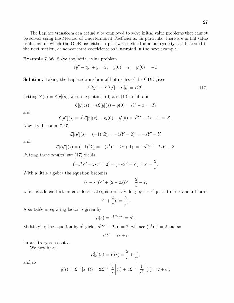
The Laplace transform can actually be employed to solve initial value problems that cannotbe solved using the Method of Undetermined Coefficients. In particular there are initial valueproblems for which the ODE has either a piecewise-defined nonhomogeneity as illustrated inthe next section, or nonconstant coefficients as illustrated in the next example.


ty′′ − ty′ + y = 2, y(0) = 2, y′(0) = −1

Solution. Taking the Laplace transform of both sides of the ODE gives

L[ty′′]− L[ty′] + L[y] = L[2]. (17)

Letting Y (s) = L[y](s), we use equations (9) and (10) to obtain

L[y′](s) = sL[y](s)− y(0) = sY − 2 := Z1

andL[y′′](s) = s2L[y](s)− sy(0)− y′(0) = s2Y − 2s+ 1 := Z2.

Now, by Theorem 7.27,

L[ty′](s) = (−1)1Z ′1 = −(sY − 2)′ = −sY ′ − Yand

L[ty′′](s) = (−1)1Z ′2 = −(s2Y − 2s+ 1)′ = −s2Y ′ − 2sY + 2.

Putting these results into (17) yields

(−s2Y ′ − 2sY + 2)− (−sY ′ − Y ) + Y =2

s.

With a little algebra the equation becomes

(s− s2)Y ′ + (2− 2s)Y =2

s− 2,

which is a linear first-order differential equation. Dividing by s− s2 puts it into standard form:

Y ′ +2

sY =

2

s2.

A suitable integrating factor is given by

µ(s) = e∫2/s ds = s2.

Multiplying the equation by s2 yields s2Y ′ + 2sY = 2, whence (s2Y )′ = 2 and so

s2Y = 2s+ c

for arbitrary constant c.We now have

L[y](s) = Y (s) =2

s+

c

s2,

and so

y(t) = L−1[Y ](t) = 2L−1[

1

s

](t) + cL−1

[1

s2

](t) = 2 + ct.

28

Thus y′(t) = c, and to determine c we must, oddly enough, make use of the initial conditiony′(0) = −1 again to obtain c = −1. Therefore

y(t) = 2− t

is the solution to the IVP. And there was much rejoicing throughout the kingdom. �

29

7.6 – Transforms of Piecewise-Defined Functions

We begin with an important discontinuous function often used to model processes thatchange suddenly in value.

Definition 7.37. The unit step function u(t) is defined by

u(t) =

{0, if t < 0

1, if t ≥ 0

Some authors have > where we have ≥, and so leave u(0) undefined; but for theoreticalreasons it makes more sense to set u(0) = 1.2 So u has a jump discontinuity at t = 0. If wewish for a function that has a jump discontinuity at t = a, we need only compose u with thefunction h(t) = t− a:

(u ◦ h)(t) = u(h(t)) = u(t− a) =

{0, if t < a

1, if t ≥ a

See Figure 3.In general, given any function f(t) : [a,∞)→ R, we define

f(t)u(t− a) =

{0, if t < a

f(t), if t ≥ a

We take this to be the case even if f(t) is undefined for t < a!

Proposition 7.38. Let f : [0,∞)→ R be a function. If a ≥ 0 and L[f(t)](s) exists for s > α,then

L[f(t− a)u(t− a)](s) = e−asL[f(t)](s) (18)

for s > α.

Proof. Suppose that a ≥ 0 and L[f(t)](s) exists for all s > α. Thus, for any real-valuedquantity c that is independent of t, we have∫ ∞

0

e−st · cf(t) dt = c

∫ ∞0

e−stf(t) dt

2Otherwise we’re left to interpret, say,∫ 2

0u(t) dt as an improper integral of the second kind, as discussed in

§7.1.

t

u(t)

1

Figure 2. The unit step function.

30

t

u(t− a)

1

a

Figure 3. The function u(t− a).

for any s > α, a result we shall make use of presently.By Definition 7.14, and making the substitution τ = t− a, we obtain

L[f(t− a)u(t− a)](s) =

∫ ∞0

e−stf(t− a)u(t− a) dt = limb→∞

∫ b

0

e−stf(t− a)u(t− a) dt

= limb→∞

∫ b

a

e−stf(t− a) dt = limb→∞

∫ b−a

0

e−s(τ+a)f(τ) dτ

= limb→∞

∫ b−a

0

e−sτ · e−saf(τ) dτ =

∫ ∞0

e−sτ · e−saf(τ) dτ

=

∫ ∞0

e−st · e−saf(t) dt = e−sa∫ ∞0

e−stf(t) dt

= e−asL[f(t)](s)

for any s > α. �

In particular if we suppose that a > 0 and f(t) ≡ 1, then from (18) we obtain

L[u(t− a)](s) = e−asL[1](s) =e−as

s.

for all s > 0, which may also be obtained easily enough from Definition 7.14.From the proposition above the following quite similar result obtains, which is needed often

in applications.

Corollary 7.39. If a > 0 and g : [a,∞) → R is a function for which L[g(t+ a)](s) exists fors > α, then

L[g(t)u(t− a)](s) = e−asL[g(t+ a)](s) (19)

for s > α.

Proof. Define f : [0,∞) → R by f(t) = g(t + a), so that g(t) = f(t− a) for t ≥ a > 0. Now,for s > α,

L[g(t)u(t− a)](s) = L[f(t− a)u(t− a)](s) = e−asL[f(t)](s) = e−asL[g(t+ a)](s),

where the second equality follows from Proposition 7.38. �

Example 7.40. Determine the Laplace transform of f(t) = 5t3u(t− 6).

31

Solution. Here we have g(t)u(t− a) with g(t) = 5t3 and a = 6. Thus

g(t+ a) = g(t+ 6) = 5(t+ 6)3,

and using (19) in the corollary gives

L[5t3u(t− 6)

](s) = e−6sL

[5(t+ 6)3

](s) = 5e−6sL

[t3 + 18t2 + 108t+ 216

](s)

Now we have

L[5t3u(t− 6)

](s) = 5e−6s

(L[t3](s) + 18L

[t2](s) + 108L[t](s) + 216L[1](s)

)= 5e−6s

(3!

s4+ 18 · 2!

s3+ 108 · 1!

s2+ 216 · 1

s

)=

(30

s4+

180

s3+

540

s2+

1080

s

)e−6s,

using linearity and Table 7.1. �

Example 7.41. Determine the inverse Laplace transform of

G(s) =e−2s

s2 + 9.

Solution. Let f(t) be the function for which L[f(t)](s) = 1/(s2 + 9). Setting a = 2 in (18)gives

L[f(t− 2)u(t− 2)](s) = e−2sF (s) = G(s). (20)

From Table 7.1 we find that

L[

1

3sin 3t

](s) =

1

3· 3

s2 + 9=

1

s2 + 9= L[f(t)](s),

so f(t) = 13

sin 3t and from (20) we obtain

L[

1

3sin(3t− 6)u(t− 2)

](s) = G(s).

Therefore

L−1[e−2s

s2 + 9

](t) =

1

3sin(3t− 6)u(t− 2).

�

Definition 7.42. Let −∞ < a < b < ∞. The rectangular window function associatedwith a and b is the function Πa,b given by

Πa,b(t) = u(t− a)− u(t− b) =

0, if t < a

1, if a ≤ t < b

0, if t ≥ b

The unit step function and rectangular window function can be employed to characterizepiecewise-defined functions using a single expression.

32

Example 7.43. To express the function

f(t) =

3t2, if t < −2

0, if −2 ≤ t < 1

2t, if 1 ≤ t < 3

t sin t, if t ≥ 3

in terms of the functions u and Π, note that

3t2 − 3t2u(t+ 2) =

{3t2 if t < −2

0, if t ≥ −2

and

2tΠ1,3(t) =

0, if t < 1

2t, if 1 ≤ t < 3

0, if t ≥ 3

and

tu(t− 3) sin t =

{0, if t < 3

t sin t, if t ≥ 3

Summing these three functions gives the desired result:

f(t) = 3t2 − 3t2u(t+ 2) + 2tΠ1,3(t) + tu(t− 3) sin t.

Notice in particular that f(−2) = 3(−2)2 − 3(−2)2 + 0 + 0 = 0, as required.If it’s desired that f be expressed exclusively in terms of u, simply observe that Π1,3(t) =

u(t− 1)− u(t− 3), and so

f(t) = 3t2 − 3t2u(t+ 2) + 2t[u(t− 1)− u(t− 3)] + tu(t− 3) sin t,

or equivalently

f(t) = 3t2 − 3t2u(t+ 2) + 2tu(t− 1) + (t sin t− 2t)u(t− 3).

�

Example 7.44. Find the Laplace transform of the function f in Example 7.43.

Solution. From the final expression for f(t) obtain above, we have

L[f ](s) = L[3t2 − 3t2u(t+ 2) + 2tu(t− 1) + (t sin t− 2t)u(t− 3)

](s)

= 3L[t2](s)− 3L

[t2u(t+ 2)

](s) + 2L[tu(t− 1)](s) + L[t sin t · u(t− 3)](s)

− 2L[tu(t− 3)](s).

We now use Table 7.1 and (19) to obtain

L[f ](s) = 3 · 2!

s2+1− 3e2sL

[(t− 2)2

](s) + 2e−sL[t+ 1](s) + e−3sL[(t+ 3) sin(t+ 3)](s)

− 2e−3sL[t+ 3](s).

33

To determine L[(t− 2)2](s) we simply expand the polynomial,

L[(t− 2)2

](s) = L

[t2 − 4t+ 4

](s) =

2

s3− 4

s2+

4

s.

As for L[(t+ 3) sin(t+ 3)](s), the trigonometric identity sin(u + v) = sinu cos v + cosu sin vwill prove useful, giving

L[(t+ 3) sin(t+ 3)](s) = L[(t+ 3)(sin t cos 3 + cos t sin 3)](s)

= (cos 3)L[t sin t](s) + (sin 3)L[t cos t](s) + (3 cos 3)L[sin t](s)

+ (3 sin 3)L[cos t](s)

=2s cos 3

(s2 + 1)2+

(s2 − 1) sin 3

(s2 + 1)2+

3 cos 3

s2 + 1+

3s sin 3

s2 + 1.

Gathering all our results, we have

L[f ](s) =6

s3− 3e2s

(2

s3− 4

s2+

4

s

)+ 2e−s

(1

s2+

1

s

)+

2s cos 3 + (s2 − 1) sin 3

(s2 + 1)2

+3 cos 3 + 3s sin 3

s2 + 1− 2e−3s

(1

s2+

3

s

),

certainly no trivial expression! �

Example 7.45. Solve the initial value problem y′′ − y = f(t), y(0) = 1, y′(0) = 2, where f isgiven by

f(t) =

{1, if 0 ≤ t < 3

t, if t ≥ 3

Solution. We start by expressing f in terms of u:

f(t) = 1 + (−1 + t)u(t− 3). (21)

Now we have y′′ − y = 1 − u(t − 3) + tu(t − 3). Taking the Laplace transform of each side,linearity properties yield

L[y′′](s)− L[y](s) = L[1](s)− L[u(t− 3)](s) + L[tu(t− 3)](s).

Now, letting Y (s) = L[y](s), by (10) and (19) we have

s2Y (s)− sy(0)− y′(0)− Y (s) =1

s− e−3s

s+ e−3sL[t+ 3](s).

Using the given initial conditions then leads to

s2Y (s)− s− 2− Y (s) =1

s− e−3s

s+ e−3s

(1

s2+

3

s

)=

1

s+ e−3s

(1

s2+

2

s

).

So the function Y can be seen to be given by

Y (s) =1

s2 − 1

(s+ 2 +

1

s+

2s+ 1

s2e−3s

)=

s+ 2

s2 − 1+

1

s(s2 − 1)+

2s+ 1

s2(s2 − 1)e−3s.

34

Partial fraction decomposition on the rightmost expression yields

Y (s) =

(3/2

s− 1− 1/2

s+ 1

)+

(−1

s+

1/2

s− 1+

1/2

s+ 1

)+

(−2

s− 1

s2+

3/2

s− 1+

1/2

s+ 1

)e−3s,

which a little algebra renders as

Y (s) =2

s− 1− 1

s− 2

se−3s − 1

s2e−3s +

3/2

s− 1e−3s − 1/2

s+ 1e−3s.

Hence

y(t) = 2L−1[

1

s− 1

](t)− L−1

[1

s

](t)− 2L−1

[1

se−3s

](t)− L−1

[1

s2e−3s

](t)

+3

2L−1

[1

s− 1e−3s

](t)− 1

2L−1

[1

s+ 1e−3s

](t).

By Table 7.1 and (18), then,

y(t) = 2et − 1− 2u(t− 3)− (t− 3)u(t− 3) +3

2et−3u(t− 3)− 1

2e3−tu(t− 3).

Therefore

y(t) = 2et − 1 +

(1− t+

3

2et−3 − 1

2e3−t

)u(t− 3)

is the solution to the initial value problem. �

The solution to the IVP in Example 7.45 is seen to be

y(t) =

{2et − 1, 0 ≤ t < 3

2et − t+ 32et−3 + 1

2e3−t, t ≥ 3

Note that the graph of y(t), shown in Figure 4, does not exhibit any manifestly unusual prop-erties at t = 3 or anywhere else! In fact the smooth appearance of the graph at t = 3 shouldlead us to wonder whether y(t) is differentiable there despite being piecewise-defined. We have

y′+(3) = limt→3+

y(t)− y(3)

t− 3= lim

t→3+

(2et − t+ 3

2et−3 + 1

2e3−t

)− (2e3 − 1)

t− 3,

t

y(t)

3

100

200

Figure 4.

35

which has a 0/0 indeterminate form and so by L’Hopital’s Rule it follows that

y′+(3)LR= lim

t→3+

(2et − 1 +

3

2et−3 − 1

2e3−t

)= 2e3.

In similar fashion we obtain

y′−(3) = limt→3−

y(t)− y(3)

t− 3= lim

t→3−

(2et − 1)− (2e3 − 1)

t− 3LR= lim

t→3−2et = 2e3.

We see that y(t) is differentiable, and thus continuous, at t = 3 with y′(3) = 2e3, and we have

y′(t) =

{2et, 0 ≤ t < 3

2et − 1 + 32et−3 − 1

2e3−t, t ≥ 3

(Since Dom(y) = [0,∞), at t = 0 there is strictly speaking a right-hand derivative y′+(0) only.)Moreover

limt→3

y′(t) = 2e3 = y′(3)

shows that y′(t) is continuous at t = 3 as well.Now we investigate the second derivative y′′(t):

y′′+(3) = limt→3+

y′(t)− y′(3)

t− 3= lim

t→3+

(2et − 1 + 3

2et−3 − 1

2e3−t

)− 2e3

t− 3

LR=

(2et +

3

2et−3 +

1

2e3−t

)= 2e3 + 2

and

y′′−(3) = limt→3−

y′(t)− y′(3)

t− 3= lim

t→3−

2et − 2e3

t− 3LR= lim

t→3−2et = 2e3

Since y′′+(3) 6= y′′−(3) we conclude that y′′(3) does not exist and so y′′(t) is not differentiable att = 3. Indeed y′′(t) has a jump discontinuity of +2 in value at t = 3 precisely as f(t) on theright-hand side of the ODE does. We have

y′′(t) =

{2et, 0 ≤ t < 3

2et + 32et−3 + 1

2e3−t, t > 3

Because 3 /∈ Dom(y′′) must we accept that y(t) is not a solution to the IVP on [0,∞), but“only” on [0, 3) ∪ (3,∞)? There are a few options. One option is the route of the engineer orphysicist: t = 3 is merely an instant in time, so we refrain from considering what is happeningto the physical system modeled by the IVP during that instant. Another option is to let y′′+(3)stand in for the value of y′′(t) at t = 3, since the result does indeed satisfy the ODE:

y′′+(3)− y(3) = f(3) ⇒ (2e3 + 2)− (2e3 − 1) = 3 ⇒ 3 = 3.

A third option adopted by some textbooks (which is really the first option writ large) is to usea version of the unit step function u(t) that is not defined at t = 0, so that f(t) given by (21)is not defined at t = 3 and we are relieved at the outset of any expectation to come up with asolution to the IVP there.3

3This third option we do not entertain for reasons mentioned at the beginning of this section.

36

7.7 – Transforms of Impulse Functions

Many physical phenomena are modeled by a differential equation of the form

any(n) + · · ·+ a2y

′′ + a1y′ + a0y = f(t),

where the nonhomogeneity f is such that

f(t) =

{M, t0 − ε < t < t0 + ε

0, otherwise

for some large M > 0 and small ε > 0. Such a function is called an impulse function, whichtypically is constant in value on the short interval (t0− ε, t0 + ε) where it is nonzero, although itis not a requirement. The total impulse of f , which could represent a force, voltage, or someother physical quantity that varies as a function of time t, is defined to be

I(f) =

∫ ∞−∞

f(t) dt =

∫ t0+ε

t0−εf(t) dt.

In particular, setting t0 = 0, we may have

f(t) = dε(t) =

{12ε, |t| < ε

0, |t| ≥ ε

in which case

I(dε) =

∫ ∞−∞

dε(t) dt =

∫ ε

−ε

1

2εdt =

1

2ε[(ε)− (−ε)] = 1

for any ε > 0. Observe that the smaller ε becomes (i.e. the shorter the time the impulseoccurs), the larger 1

2εbecomes (i.e. the greater the magnitude of the impulse), with the net

effect being a total impulse of 1. The function dε is called a unit impulse function.As ε tends to zero, we find that dε approaches a kind of idealized unit impulse function that

occurs “instantaneously” at t = 0 and has “infinite” magnitude. We have

limε→0+

dε(t) = 0 (22)

for all t 6= 0, and also

limε→0+

I(dε) = limε→0+

∫ ∞−∞

dε(t) dt = limε→0+

∫ ε

−εdε(t) dt = lim

ε→0+(1) = 1. (23)

Equations (22) and (23) serve as motivation for the following definition.

Definition 7.46. The Dirac delta is the idealized unit impulse function δ given by δ(t) = 0for all t 6= 0, and with the formal property∫ ∞

−∞δ(t) dt = 1. (24)

The Dirac delta is not a function in the conventional sense. No conventional function f canbe zero everywhere except at one point, and yet manage to have a nonzero proper or improper

Riemann integral∫ baf for some choice of limits a and b. Rigorous justification of the Dirac

delta is beyond the scope of this text. For our purposes the Dirac delta is a formal device

37

that enables us to conveniently—and accurately—model physical systems involving impulsefunctions. If t0 6= 0, then an immediate consequence of Definition 7.46 is that

δ(t− t0) = 0, t 6= t0, (25)

and ∫ ∞−∞

δ(t− t0) dt = 1.

Since

dε(t− t0) =

{12ε, t0 − ε < t < t0 + ε

0, t ≤ t0 − ε or t ≥ t0 + ε

we see from (25) that

δ(t− t0) = limε→0+

dε(t− t0),

which motives yet another formal definition.

Definition 7.47. For t0 > 0 we define

L[δ(t− t0)](s) = limε→0+

L[dε(t− t0)](s).

Theorem 7.48. If t0 > 0, then

L[δ(t− t0)](s) = e−st0 .

Proof. Let t0 > 0. Then there exists ε > 0 sufficiently small that t0 − ε > 0, and so

L[dε(t− t0)](s) =

∫ ∞0

e−stdε(t− t0) dt =

∫ t0+ε

t0−ε

e−st

2εdt

=1

2ε

[−1

se−st

]t0+εt0−ε

= − 1

2εs

[e−s(t0+ε) − e−s(t0−ε)

].

Now, by Definition 7.47

L[δ(t− t0)](s) = limε→0+

L[dε(t− t0)](s) = limε→0+

e−st0

2

(esε − e−sε

sε

),

and since the limit at right has indeterminate form 0/0 we may apply L’Hopital’s Rule (differ-entiating with respect to ε) to obtain

L[δ(t− t0)](s) = limε→0+

e−st0

2

(sesε + se−sε

s

)= lim

ε→0+

e−st0

2

(esε + e−sε

)=e−st0

2

(e0 + e0

)= e−st0 ,

as was to be shown. �

We can extend the result of Theorem 7.48 to the case when t0 = 0 with a natural definition:

L[δ(t)](s) := limt0→0

e−st0 = 1 (26)

for all s ∈ [0,∞).Generalizing the spirit of Definition 7.47, we have the following.

38

Definition 7.49. If f is a continuous function, then∫ ∞−∞

f(t)δ(t− t0) dt = limε→0+

∫ ∞−∞

f(t)dε(t− t0) dt

for any t0 ∈ R.

Theorem 7.50. If f is continuous and t0 ∈ R, then∫ ∞−∞

f(t)δ(t− t0) dt = f(t0). (27)

Proof. Suppose that f : R→ R is continuous and t0 ∈ R. We have

limε→0+

∫ ∞−∞

f(t)dε(t− t0) dt = limε→0+

∫ t0+ε

t0−εf(t) · 1

2εdt = lim

ε→0+

1

2ε

∫ t0+ε

t0−εf(t) dt. (28)

Now, by the Mean Value Theorem for Integrals4 there exists some t∗ε ∈ (t0 − ε, t0 + ε), whichdepends on ε, such that

f(t∗ε) =1

(t0 + ε)− (t0 − ε)

∫ t0+ε

t0−εf(t) dt,

and thus ∫ t0+ε

t0−εf(t) dt = 2εf(t∗ε).

Returning to (28),

limε→0+

∫ ∞−∞

f(t)dε(t− t0) dt = limε→0+

(1

2ε· 2εf(t∗ε)

)= lim

ε→0+f(t∗ε).

Let α > 0 be arbitrary. Since f is continuous at t0, there exists some β > 0 such that

|t− t0| < β ⇒ |f(t)− f(t0)| < α

Suppose that ε > 0 is such that ε < β. Then

t∗ε ∈ (t0 − ε, t0 + ε) ⊆ (t0 − β, t0 + β),

which is to say |t∗ε − t0| < β and so ∣∣f(t∗ε)− f(t0)∣∣ < α.

This shows thatlimε→0+

f(t∗ε) = f(t0),

and therefore

limε→0+

∫ ∞−∞

f(t)dε(t− t0) dt = f(t0).

Now (27) follows by Definition 7.49. �


y′′ + 4y = 2δ(t− π)− δ(t− 2π), y(0) = 0, y′(0) = 0.

4See §6.1 of [CAL].

http://faculty.bucks.edu/erickson/math140/140chap6.pdf

39

Solution. We take the Laplace transform of each side of the ODE, using linearity propertiesto obtain

L[y′′](s) + 4L[y](s) = 2L[δ(t− π)](s)− L[δ(t− 2π)](s).

Now, letting Y (s) = L[y](s) and using Theorem 7.48, we obtain

[s2Y (s)− sy(0)− y′(0)] + 4Y (s) = 2e−πs − e−2πs,whence

Y (s) =2e−πs

s2 + 4− e−2πs

s2 + 4and so

y(t) = L−1[

2e−πs

s2 + 4

](t)− L−1

[e−2πs

s2 + 4

](t). (29)

If we define h(t) = sin(2t), then

L[h(t)](s) =2

s2 + 4,

so by Proposition 7.38

L[h(t− π)u(t− π)](s) = e−πsL[h(t)](s) =2e−πs

s2 + 4

and hence

L−1[

2e−πs

s2 + 4

](t) = h(t− π)u(t− π) = sin(2t− 2π)u(t− π) = sin(2t)u(t− π).

In similar fashion we obtain

L−1[e−2πs

s2 + 4

](t) =

1

2h(t− 2π)u(t− 2π) =

1

2sin(2t− 4π)u(t− 2π) =

1

2sin(2t)u(t− 2π).


y(t) = sin(2t)[u(t− π)− 1

2u(t− 2π)

],

t

y(t)

π 2π 3π

12

1

Figure 5.

40

or equivalently

y(t) =

0, 0 ≤ t < π

sin(2t), π ≤ t < 2π12

sin(2t), t ≥ 2π

See Figure 5 for the graph of y(t). �


y′′ + y′ + 2y = 5δ(t− 3), y(0) = 0, y′(0) = 1.

Solution. We take the Laplace transform of each side of the ODE, using linearity propertiesto obtain

L[y′′](s) + L[y′](s) + 2L[y](s) = 5L[δ(t− 3)](s).

Letting Y (s) = L[y](s) and using Theorem 7.48, we obtain

[s2Y (s)− sy(0)− y′(0)] + [sY (s)− y(0)] + 2Y (s) = 5e−3s,

whence

[s2Y (s)− 1] + sY (s) + 2Y (s) = 5e−3s ⇒ Y (s) =1 + 5e−3s

s2 + s+ 2.

Since s2 + s+ 2 is an irreducible quadratic, we cast it as a sum of squares:

s2 + s+ 2 =[s2 + s+

(12

)2]+ 2−

(12

)2=(s+ 1

2

)2+(√

72

)2.

From

Y (s) =1

(s+ 1/2)2 + 7/4+

5e−3s

(s+ 1/2)2 + 7/4

we obtain

y(t) = L−1[

1

(s+ 1/2)2 + 7/4

](t) + 5L−1

[e−3s

(s+ 1/2)2 + 7/4

](t). (30)

Referring to Table 1, we find that

L−1[

1

(s+ 1/2)2 + 7/4

](t) =

2√7L−1

[ √7/2

(s+ 1/2)2 +(√

7/2)2]

(t) =2√7e−t/2 sin

(√7t/2

).

Now, if we let

h(t) =2√7e−t/2 sin

(√7t/2

),

then by Proposition 7.38

L[h(t− 3)u(t− 3)](s) = e−3sL[h(t)](s) =e−3s

(s+ 1/2)2 + 7/4

and thus

L−1[

e−3s

(s+ 1/2)2 + 7/4

](t) = h(t− 3)u(t− 3) =

2√7e−(t−3)/2 sin

(√7(t− 3)/2

)u(t− 3).

41

t

y(t)

2 4 6 8 10

1

2

Figure 6.


y(t) =2√7e−t/2 sin

(√7t/2

)+

10√7e−(t−3)/2 sin

(√7(t− 3)/2

)u(t− 3),

the graph of which is presented in Figure 6. �


y′′ + y = δ(t− 2π) cos(t), y(0) = 0, y′(0) = 1.

Solution. We take the Laplace transform of each side of the ODE, using linearity propertiesand letting Y (s) = L[y(t)](s) to obtain

[s2Y (s)− sy(0)− y′(0)] + Y (s) = L[δ(t− 2π) cos(t)](s). (31)

Since δ(t− 2π) = 0 for all t < 0, we have∫ ∞0

e−stδ(t− 2π) cos(t) dt =

∫ ∞−∞

e−stδ(t− 2π) cos(t) dt,

and so by Theorem 7.50

L[δ(t− 2π) cos(t)](s) =

∫ ∞−∞

e−stδ(t− 2π) cos(t) dt = e−2πs cos(2π) = e−2πs.

Equation (31) now becomes[s2Y (s)− 1] + Y (s) = e−2πs,

whence

Y (s) =1

s2 + 1+

e−2πs

s2 + 1,

and finally

y(t) = L−1[

1

s2 + 1

](t) + L−1

[e−2πs

s2 + 1

](t).

With Table 1 and Proposition 7.38 we obtain

y(t) = sin(t) + sin(t− 2π)u(t− 2π),

42

t

y(t)

π 2π 3π

2

1

−1

Figure 7.

or simplyy(t) = sin(t)[1 + u(t− 2π)]


43

7.8 – Convolution

Definition 7.54. Let f, g be piecewise continuous on [0,∞). The convolution of f and g isthe function f ∗ g : [0,∞)→ R given by

(f ∗ g)(t) =

∫ t

0

f(t− τ)g(τ) dτ.

Proposition 7.55. If f, g, h are piecewise continuous on [0,∞), then

1. f ∗ g = g ∗ f2. f ∗ (g + h) = f ∗ g + f ∗ h3. f ∗ (g ∗ h) = (f ∗ g) ∗ h4. f ∗ 0 = 0

Theorem 7.56 (Convolution Theorem). If f, g are piecewise continuous on [0,∞) and ofexponential order α, then

L[f ∗ g](s) = L[f ](s)L[g](s).

for all s > α.

If we set F (s) = L[f ](s) and G(s) = L[g](s), then

L[f ∗ g](s) = F (s)G(s) ⇒ L−1[F (s)G(s)](t) = (f ∗ g)(t)

derives from the Convolution Theorem.

Example 7.57. Use the Convolution Theorem to find the inverse Laplace transform of

H(s) =s

(s2 + 1)2.

Solution. We have

L−1[H(s)](t) = L−1[

s

(s2 + 1)2

](t) = L−1

[s

s2 + 1· 1

s2 + 1

](t) = L−1[F (s)G(s)](t)

where

F (s) =s

s2 + 1and G(s) =

1

s2 + 1.

Letting f(t) = cos t and g(t) = sin t, we readily see that F (s) = L[f ](s) and G(s) = L[g](s),and therefore

L−1[H(s)](t) = L−1[F (s)G(s)](t) = (f ∗ g)(t) = (cos ∗ sin)(t).

That is,

L−1[H(s)](t) = (cos ∗ sin)(t) =

∫ t

0

cos(t− τ) sin(τ) dτ,

and so using the trigonometric identity

sinx cos y =1

2[sin(x+ y) + sin(x− y)]

44

we obtain

L−1[H(s)](t) =1

2

∫ t

0

[sin t+ sin(2τ − t)] dτ =1

2

[τ sin t− 1

2cos(2τ − t)

]t0

=1

2

[(t sin t− 1

2cos t

)−(

0− 1

2cos(−t)

)]=

1

2t sin t.

�

Example 7.58. Solve the integral equation

y(t) +

∫ t

0

(t− τ)2y(τ) dτ = t3 + 3.

Solution. We have ∫ t

0

(t− τ)2y(τ) dτ = (f ∗ g)(t)

with f(t) = t2 and g(t) = y(t), so the integral equation may be written as

y(t) + (f ∗ y)(t) = t3 + 3.

Taking the Laplace transform of both sides of the equation yields, by the Convolution Theorem,

L[y](s) + L[f ](s)L[y](s) = L[t3](s) + L[3](s),

orY (s) + Y (s)L

[t2](s) = L

[t3](s) + L[3](s)

if we let Y (s) = L[y](s). Using a table of Laplace transforms yields

Y (s) + Y (s) · 2

s3=

6

s4+

3

s⇒ Y (s)

(2 + s3

s3

)=

3(2 + s3)

s4⇒ Y (s) =

3

s,

whence

y(t) = L−1[

3

s

](t) = 3

obtains as the (unique) solution. �

45

A Table of Laplace Transforms

f(t) L[f ](s) Dom(L[f ])

t sin bt2bs

(s2 + b2)2s > 0

t cos bts2 − b2

(s2 + b2)2s > 0

eat sin btb

(s− a)2 + b2s > a

eat cos bts− a

(s− a)2 + b2s > a

eattn, n = 0, 1, . . .n!

(s− a)n+1s > a

u(t− a), a ≥ 0e−as

ss > 0

δ(t− a), a ≥ 0 e−as s > 0

(f ∗ g)(t) L[f(t)](s)L[g(t)](s) s > 0

1√t

√π

ss > 0

√t

1

2s

√π

ss > 0

tn−1/2, n = 1, 2, . . .1 · 3 · 5 · · · (2n− 1)

√π

2nsn+1/2s > 0

Documents

7.1 { Improper Riemann Integrals - Bucks County Community College