7. The Aggregate Supply Curve Abel, Bernanke, and Croushore (chapters 3 and 9.6)

7. The Aggregate Supply Curve

Abel, Bernanke, and Croushore (chapters 3 and 9.6)

Syllabus Outline

1. Introduction to Macroeconomics

2. The measurement and structure of the national economy

3. Goods market equilibrium: the IS curve

4. Money market equilibrium: the LM curve

5. The IS-LM model

6. Demand-side policies in the IS-LM model (Keynesian Macroeconomics)

7. The Aggregate Supply curve

8. Classical Macroeconomics in the AD-AS model

9. Keynesian Macroeconomics in the AD-AS model

10. The relationship between Unemployment and Inflation

Our goals in this chapter

A) Introduce the production function as the main determinant of output 1. Discuss the marginal productivity of labor and capital 2. Analyze supply shocks

B) Discuss the determinants of labor demand and supplyC) Equilibrium in the classical model of the labor market

1. Full-employment output 2. Factors that change equilibrium

D) Unemployment 1. Definitions of employment status 2. Frictional, structural, cyclical unemployment 3. Okun’s Law

E) Aggregate Demand and Aggregate Supply

A) Factors of production

B) The production function

C) Application: The production function of the U.S. economy and U.S. productivity growth

D) The shape of the production function

E) Supply shocks

How Much Does the Economy Produce? The Production Function

A) Factors of production1. Capital2. Labor3. Others (raw materials, land, energy)4. Productivity of factors depends on technology and management

B) The production function

Y = A . F(K, N)

Y = real output produced in a given period of time A = “total factor productivity” (TECHNOLOGY index, productivity in textbook) K = capital stock, or quantity of capital used in the period N = number of workers employed in the period F = a function relating output Y to capital K and labor N


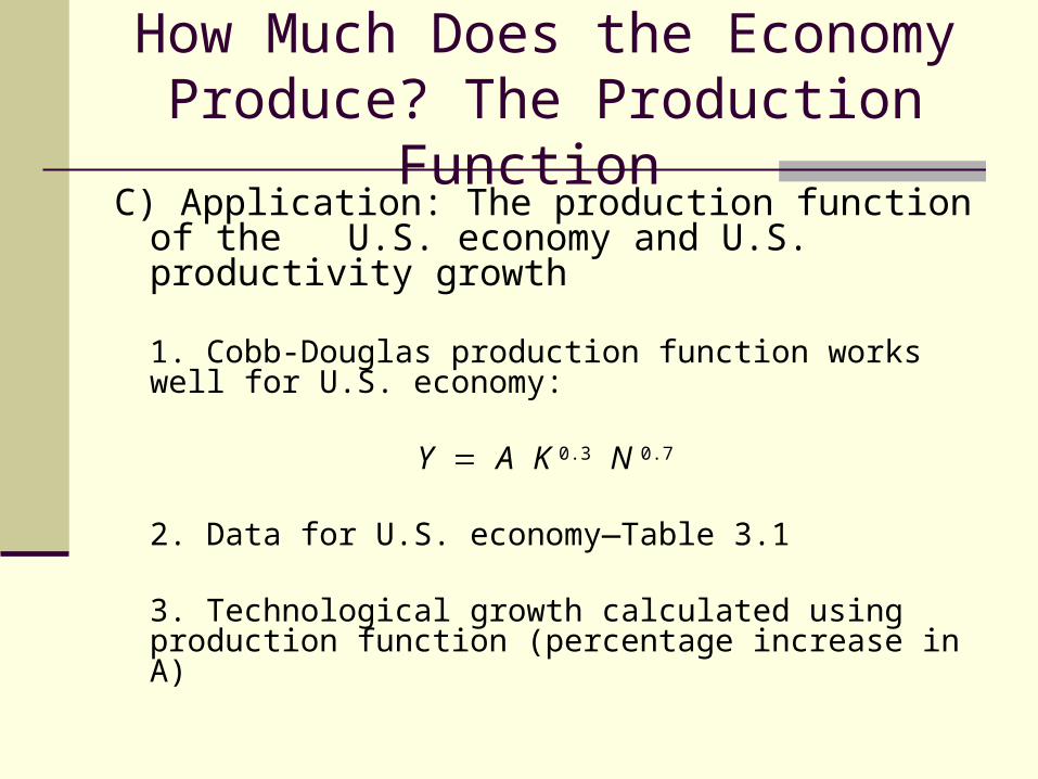
C) Application: The production function of the U.S. economy and U.S. productivity growth

1. Cobb-Douglas production function works well for U.S. economy:

Y A K 0.3 N 0.7

2. Data for U.S. economy—Table 3.1

3. Technological growth calculated using production function (percentage increase in A)


Y A K 0.3 N 0.7

Table 3.1 The Production Function of the United States, 1980–2001

3. Technological growth calculated using production function:

a. Technology index , A, is measured indirectly by assigning to A the value necessary to satisfy the previous equation

A = Y / (K 0.3 N 0.7)

b. Technology index, A, moves sharply from year to year

c. Technology index grew slowly in the 1980s and the first half of the 1990s, but increased in the second half of the 1990s


Y A K 0.3 N 0.7


1. Two main properties of production functions

a. Slopes upward: more of any input produces more output

b. Slope becomes flatter as input rises: diminishing marginal product as input increases

2. Graph of the production function


Y A K 0.3 N 0.7

Figure 3.1 The production function relating output and capital



a. Marginal product of capital MPK Y/K,


(1) Equal to slope of production function graph (Y vs. K)

(2) MPK always positive

(3) Diminishing marginal productivity of capital

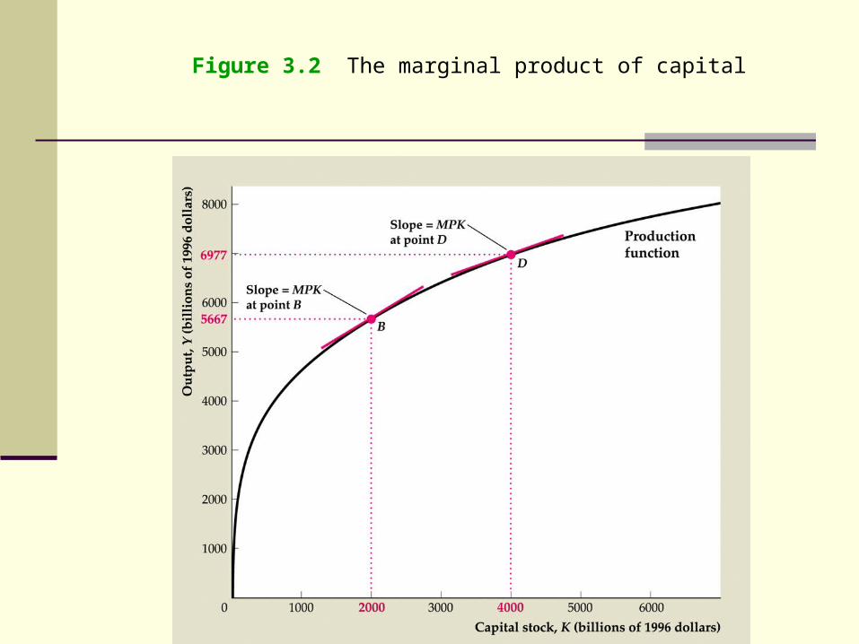
Figure 3.2 The marginal product of capital



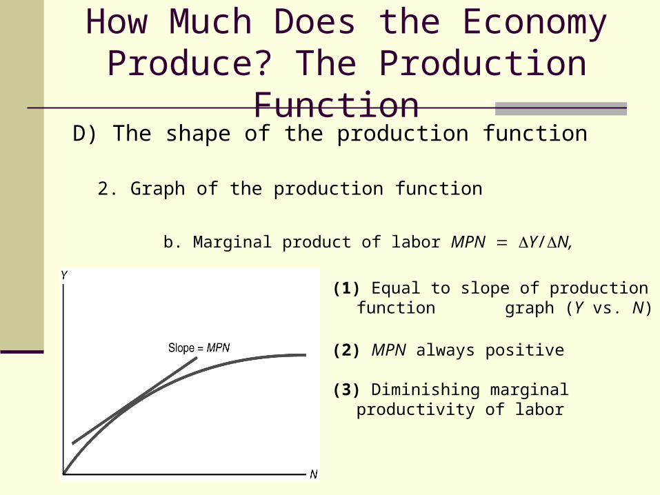
b. Marginal product of labor MPN Y/N,


(1) Equal to slope of production function graph (Y vs. N)

(2) MPN always positive

(3) Diminishing marginal productivity of labor

Figure 3.3 The production function relating output and labor

E) Supply shocks

1. Supply shocks affect the amount of output that can be produced for a given amount of inputs

2. Shocks may be positive (increasing output) or negative (decreasing output)

3. Examples: weather, inventions and innovations, government regulations, oil prices

4. Supply shocks shift graph of production function


Y A K 0.3 N 0.7

E) Supply shocks

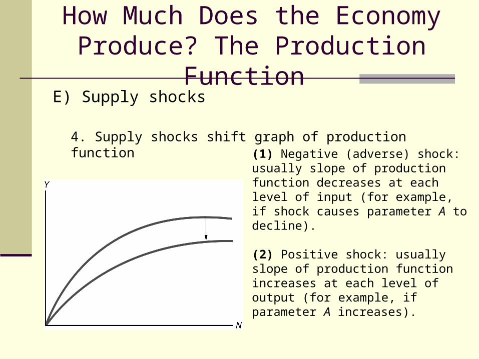
4. Supply shocks shift graph of production function


Y A K 0.3 N 0.7 (1) Negative (adverse) shock: usually slope of production function decreases at each level of input (for example, if shock causes parameter A to decline).

(2) Positive shock: usually slope of production function increases at each level of output (for example, if parameter A increases).

Figure 3.4 An adverse supply shock that lowers the MPN

A) How much labor do firms want to use?

B) The marginal product of labor and labor demand: an example

C) The marginal product of labor and the labor demand curve

D) Factors that shift the labor demand curve

E) Aggregate Labor Demand

The Demand for Labor


1. Assumptions

a. Hold capital stock fixed—short-run analysis

b. Workers are all alike

c. Labor market is competitive

d. Firms maximize profits

2. Analysis at the margin: costs and benefits of hiring one extra worker



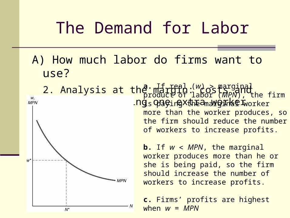
2. Analysis at the margin: costs and benefits of hiring one extra worker


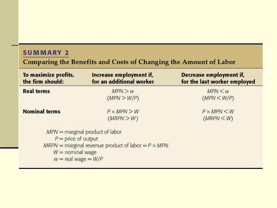
a. If real (w) marginal product of labor (MPN), the firm is paying the marginal worker more than the worker produces, so the firm should reduce the number of workers to increase profits.

b. If w MPN, the marginal worker produces more than he or she is being paid, so the firm should increase the number of workers to increase profits.

c. Firms’ profits are highest when w = MPN

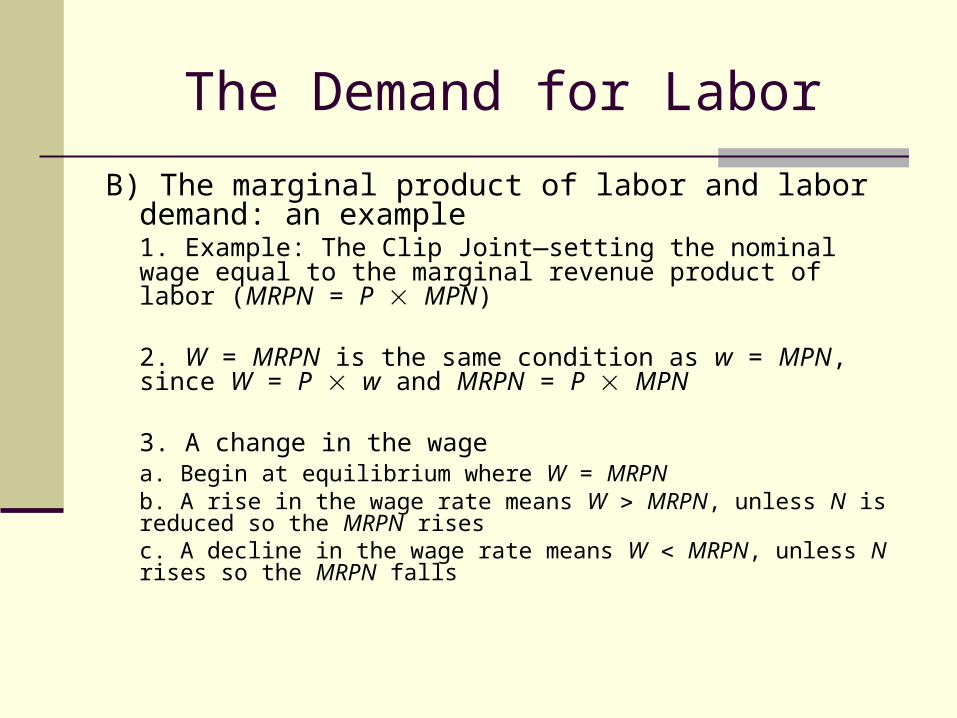
B) The marginal product of labor and labor demand: an example1. Example: The Clip Joint—setting the nominal wage equal to the marginal revenue product of labor (MRPN = P MPN)

2. W = MRPN is the same condition as w = MPN, since W = P w and MRPN = P MPN

3. A change in the wagea. Begin at equilibrium where W = MRPNb. A rise in the wage rate means W MRPN, unless N is reduced so the MRPN risesc. A decline in the wage rate means W MRPN, unless N rises so the MRPN falls


Table 3.2 The Clip Joint’s Production Function

C) The marginal product of labor and the labor demand curve

1. Labor demand curve shows relationship between the real wage rate and the quantity of labor demanded

2. It is the same as the MPN curve, since w = MPN at equilibrium

3. So the labor demand curve is downward sloping; firms want to hire less labor, the

higher the real wage


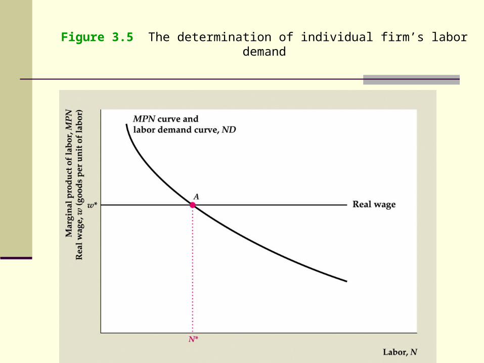
Figure 3.5 The determination of individual firm’s labor demand

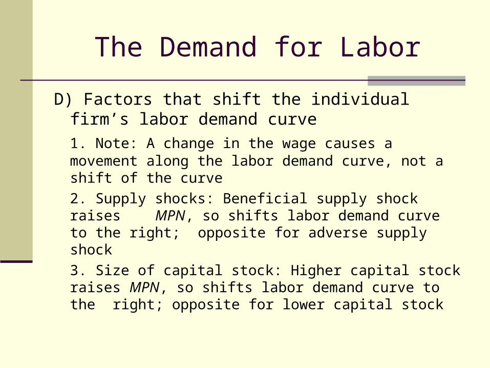
D) Factors that shift the individual firm’s labor demand curve

1. Note: A change in the wage causes a movement along the labor demand curve, not a

shift of the curve

2. Supply shocks: Beneficial supply shock raises MPN, so shifts labor demand curve to the right; opposite for adverse supply shock

3. Size of capital stock: Higher capital stock raises MPN, so shifts labor demand curve to

the right; opposite for lower capital stock


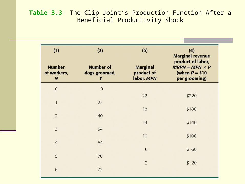
Table 3.3 The Clip Joint’s Production Function After a Beneficial Productivity Shock

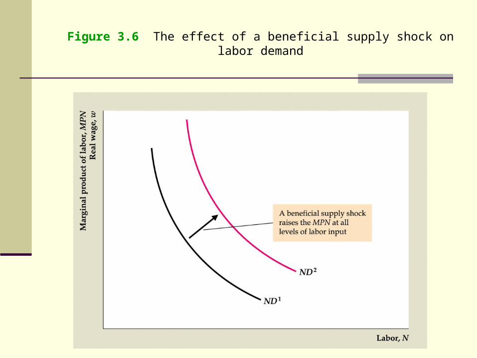
Figure 3.6 The effect of a beneficial supply shock on labor demand

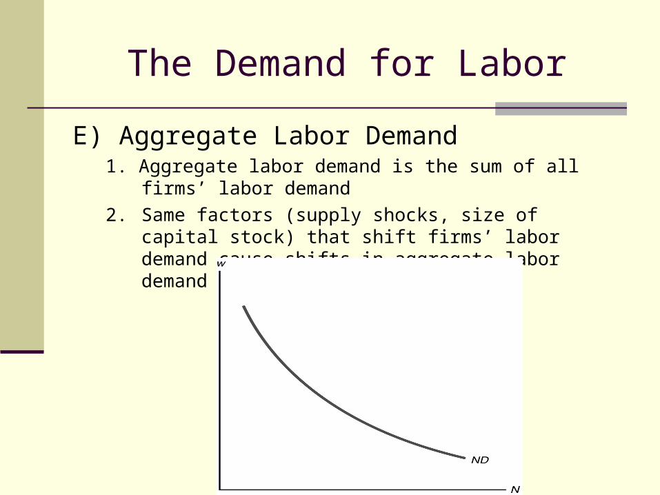
E) Aggregate Labor Demand1. Aggregate labor demand is the sum of all firms’ labor

demand

2. Same factors (supply shocks, size of capital stock) that shift firms’ labor demand cause shifts in aggregate labor demand


The Supply for Labor

A) Supply of labor is determined by individuals

B) The income-leisure trade-off

C) Real wages and labor supply

D) The labor supply curve

E) Factors that shift the labor supply curve

F) Aggregate labor supply

G) Application: weekly hours of work and the wealth of nations

The Supply for LaborA) Supply of labor is determined by individuals

1. Aggregate supply of labor is sum of individuals’ labor supply

2. Labor supply of individuals depends on labor- leisure choice

B) The income-leisure trade-off

1. Utility depends on consumption and leisure

2. Need to compare costs and benefits of working another

day

a. Costs: Loss of leisure time

b. Benefits: More consumption, since income is higher

3. If benefits of working another day exceed costs, work another day

4. Keep working additional days until benefits equal costs


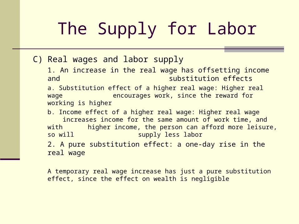
C) Real wages and labor supply1. An increase in the real wage has offsetting income and substitution effects

a. Substitution effect of a higher real wage: Higher real wage encourages work, since the reward for working is

higher

b. Income effect of a higher real wage: Higher real wage increases income for the same amount of work

time, and with higher income, the person can afford more leisure, so will supply less labor

2. A pure substitution effect: a one-day rise in the real wage

A temporary real wage increase has just a pure substitution effect, since the effect on wealth is negligible

The Supply for LaborC) Real wages and labor supply

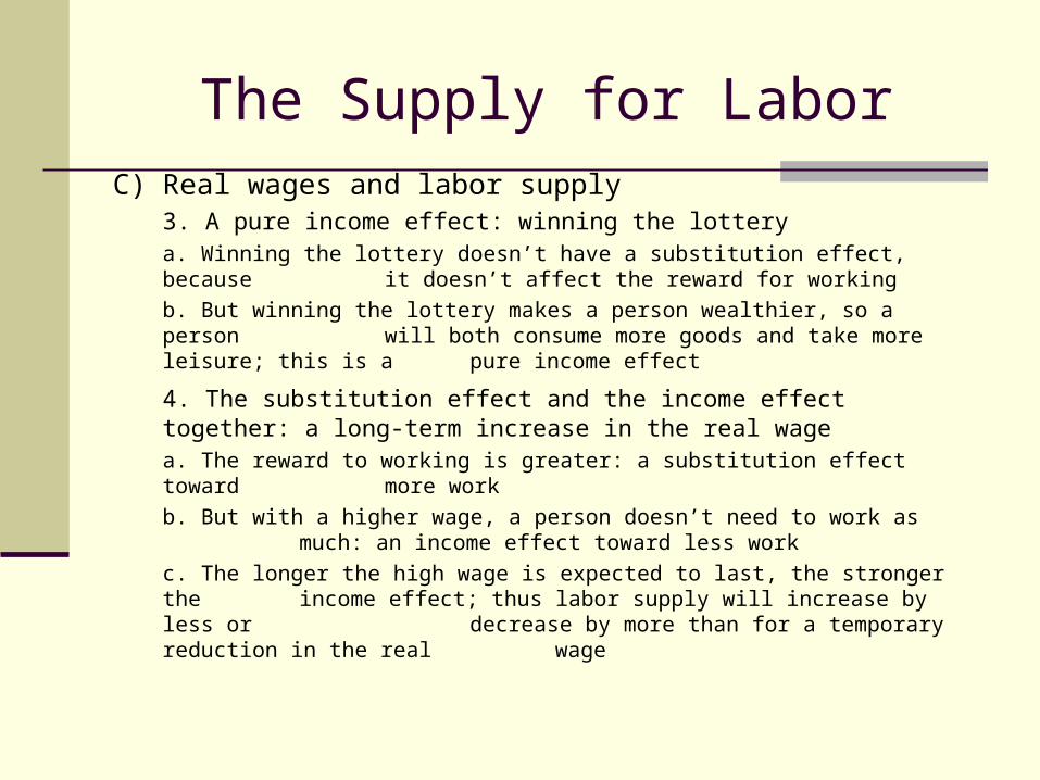
3. A pure income effect: winning the lotterya. Winning the lottery doesn’t have a substitution effect, because

it doesn’t affect the reward for working

b. But winning the lottery makes a person wealthier, so a person will both consume more goods and take more leisure; this is a pure income effect

4. The substitution effect and the income effect together: a long-term increase in the real wage

a. The reward to working is greater: a substitution effect toward more work

b. But with a higher wage, a person doesn’t need to work as much: an income effect toward less work

c. The longer the high wage is expected to last, the stronger the income effect; thus labor supply will increase by less or decrease by more than for a temporary reduction in the real wage


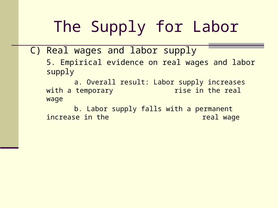
C) Real wages and labor supply5. Empirical evidence on real wages and labor supply

a. Overall result: Labor supply increases with a temporary rise in the real wage

b. Labor supply falls with a permanent increase in the real wage

Equilibrium in the Labor Market: The FE Line.

Equilibrium in the labor market leads to employment at its full-employment level (Nbar) and output at its full-employment level (Ybar)

If we plot output against the price level, we get a vertical line, since labor market equilibrium is unaffected by changes in the price level

This is the FE line Also known as the LRAS line If the economy is not producing at Ybar, eventually it

will return to this full-employment level of output

Factors that shift the FE/LRAS line

The full-employment level of output is determined by the full-employment level of employment and the current levels of capital (K) and technology (A).

any change in these variables shifts the FE/LRAS line

Documents

7. The Aggregate Supply Curve Abel, Bernanke, and Croushore (chapters 3 and 9.6)