7. Exact diagonalization

7.1 Hamiltonian operators for strongly correlated electron systems

7.1.1 The Hubbard model

The Hubbard model represents interacting electrons in narrow bands.

It was originally proposed to study metal-insulator transitions and ferro-

magnetism of itinerant electrons in narrow bands but it has also acquired

importance in the study of high temperature superconductors. Assuming

localized orbitals and a strong screening of the Coulomb interaction, only

the local density-density repulsion is included. The model is defined by

H = −t∑

<i,j>,σ

a†iσajσ

︸ ︷︷ ︸+U∑

i

ni↓ni↑

︸ ︷︷ ︸−µN

H0 H1 (7.1)

where a†iσ(aiσ) create (annihilate) fermions of spin σ =↓, ↑ in a Wannier

orbital centered at site i. niσ = a†iσaiσ represents the occupation num-

ber operator. The electrons move in tight binding bands, with a transfer

integral t between nearest neighbor sites, as indicated by < i, j >. The

Coulomb interaction strength is U. The chemical potential µ couples to

the particle number operator N =∑i(ni↓ + ni↑).

7.1.2 The t-J model

The t-J model consists of a constrained hopping term for the charge

degrees of freedom, allowing no double occupancies. It can be derived as

strong U limit of the Hubbard model. In the restricted space the eliminated

double occupancies result in an effective spin-spin interaction:

H = t∑

<i,j>,σ

(1 − ni−σ)a†iσajσ(1 − nj−σ) + J

∑

<i,j>

(SiSj −

ninj

4

)(7.2)

The projection operators (1 − ni−σ) in the kinetic term ensure that no

site is occupied by more than two electrons. The spin operators at site i

61

are Si =∑σσ ′ a

†iσσσσ ′a

†iσ ′ with Pauli matrices σσσ ′. Si describes magnetic

moments with S = 1/2 for occupied sites and S = 0 for empty sites. The

t-J model can be viewed as a generic model for the interplay of spin and

charge degrees of freedom.

7.1.3 The Heisenberg model

While the Hubbard type models treat itinerant electrons, the Heisenberg

Hamiltonian describes the situation that the charge degrees of freedom

are bound to the atomic positions and only the spin degrees of freedom

remain active. This fundamental model in the theory of magnetism of local

magnetic moments is defined by

H =∑

ij

JzijSziSzj + J

⊥ij(S

xiSxj + S

yi Syj ) + B

∑

i

Szi (7.3)

where Sαi ,α = x,y, z is the α component of the spin operator and J stands

for the exchange integrals. The last term describes the coupling to an exter-

nal magnetic field B in z direction. Special cases are the isotropic Heisen-

berg model Jz = J⊥, the Ising model J⊥ = 0 and the XY model Jz = 0.

The spin operators obey

[Sαi ,Sβj ] = iδijεαβγSγi (7.4)

For numerical purposes it is convenient to use ladder operators

S±i = Sxi ± i Syi (7.5)

so that the operators Sx and Sy can be written as

Sxi =1

2(S+i + S−i ) Syi =

1

2i(S+i − S−i ) (7.6)

Replacing Sx and Sy in the Hamiltonian leads to

H =∑

i 6=j

(JzijS

ziSzj +

1

2(S+i S

−j + S−i S

+j ))+ B∑

i

Szi (7.7)

7.2 Principle of the exact diagonalization method

To see why we have to employ special methods to make the diagonalization

of Hamilton matrices possible, we have to consider the dimension of the

62

Hamilton matrix produced by a given lattice and model.

If we study the Heisenberg Hamiltonian on a lattice of N sites, we have

two possible states for each site: Spin up and spin down. Thus the lattice

has 2N states, and this is the dimension of the Hamilton matrix. Similarly

we find for the t-J model 3N states and for the Hubbard model 4N states.

This exponential growth of the matrix with lattice size makes even small

lattices of typically 10 sites difficult to handle with standard diagonaliza-

tion techniques.

In order to make the matrix size for a given lattice size accessible to the

available computing power, it is important to exploit the model symme-

tries.

Many models, including those given above, show conservation of total spin

number, total spin in the z direction and total charge, i.e.

[H, S2

]=[H,Sz

]= [H, N] = 0 (7.8)

where H is the model Hamiltonian and

S =∑

i

Si N =∑

i

ni (7.9)

In addition, these operators also commute with each other

[S2,Sz

]=[Sz, N

]= [N, S2] = 0 (7.10)

so that the eigenvalues of H, S2, Sz and N are simultaneous good quantum

numbers which we can denote by E, S(S+ 1), Sz and N.

In order to build the Hamilton matrix, we have to choose a basis set that is

easily generated, allows fast computation of matrix elements, is economical

with memory and allows us to access states quickly. We also have to find

a numerical representation of the basis set.

For representing spin-1/2 systems, we can use integers ni = (σi+1)/2 ∈{0, 1}. If we identify the sequence of ni values with the bit pattern of the

integer I =∑Nl=1 nl2

l−1, the basis state |ψ〉 = | − 1,+1,−1,+1〉 is repre-

sented by n = {0101} and mapped onto I = 4. This representation saves

memory and speeds up some numerical operations.

As Sz =∑Ni=1 S

zi commutes with the Hamiltonian, the Hamilton matrix is

block diagonal in the sectors with fixed Sz values, i.e. fixed numbers Nσ of

σ spins.

63

For a given Sz sector, the number of ones in the bit pattern is fixed which

reduces the number of basis states to

L =

(N

N↑

)(7.11)

where N is the number of lattice sites and

Sz =1

2

(2N↑ −N

)(7.12)

For example, if the number of sites isN = 16 there are 216 = 65536 possible

basis states in total, but only

(16

8

)= 12870 for Sz = 0, i.e. N↑ = N↓ = 8.

In principle, translation and rotation could be exploited to reduce the num-

ber of basis states even further.

Now we are ready to list all permissible configurations. Not every integer is

included since the number of ones and zeros in the bit pattern is fixed. We

generate the basis states in such a way that the corresponding integer values

are in increasing order. The basis states and their integer representations

are therefore

N−N↑ N↑

|φ1〉 = {︷ ︸︸ ︷0, 0, . . . , 0, 0,

︷ ︸︸ ︷1, 1, 1, . . . , 1}; I1 = 2N

↑− 1

|φ2〉 = {0, 0, . . . , 0, 1, 0, 1, 1, . . . , 1}; I2 = 2N↑+1 − 1 − 2N

↑−1

|φ3〉 = {0, 0, . . . , 0, 1, 1, 0, 1, . . . , 1}; I3 = 2N↑+1 − 1 − 2N

↑−2

......

|φL〉 = {1, 1, . . . , 1, 1︸ ︷︷ ︸, 0, 0, 0, . . . , 0︸ ︷︷ ︸}; IL = 2N − 2N−N↑

N↑ N−N↑ (7.13)

Consider a four site cluster with Sz = 0 as an example:number 1 2 3 4 5 6

bit 0011 0101 0100 1001 1010 1100

integer 3 5 6 9 10 12As the basis states are ordered, their spin representations can be found

rapidly by bisection search.

Representation of electronic systems: The basis for Hubbard, Anderson

or t-J Hamiltonians can be conveniently constructed in real space. Restrict-

ing the discussion to a single orbital per lattice site, the state vector can

64

be writen as

|ψ〉 =N↑∏

i=1

a†Γ↑i

N↓∏

j=1

a†Γ↓j

|0〉 (7.14)

where |0〉 denotes the vacuum state and Γ ↑i is the lattice site of the i-th

spin up electron and Γ ↓j is the lattice site of the j-th spin down electron.

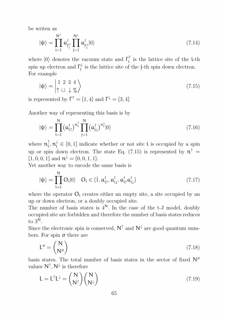
For example

|ψ〉 =∣∣∣∣

1 2 3 4

↑ t ↓ ↑↓

⟩(7.15)

is represented by Γ ↑ = {1, 4} and Γ ↓ = {3, 4}

Another way of representing this basis is by

|ψ〉 =N∏

i=1

(a†i↑)n↑i

N∏

j=1

(a†j↓)n↓j |0〉 (7.16)

where n↑i ,n↓j ∈ {0, 1} indicate whether or not site i is occupied by a spin

up or spin down electron. The state Eq. (7.15) is represented by n↑ ={1, 0, 0, 1} and n↓ = {0, 0, 1, 1}.

Yet another way to encode the same basis is

|ψ〉 =N∏

i=1

Oi|0〉 Oi ∈ {1,a†i↑,a†i↓,a

†i↑a†i↓} (7.17)

where the operator Oi creates either an empty site, a site occupied by an

up or down electron, or a doubly occupied site.

The number of basis states is 4N. In the case of the t-J model, doubly

occupied site are forbidden and therefore the number of basis states reduces

to 3N.

Since the electronic spin is conserved, N↑ and N↓ are good quantum num-

bers. For spin σ there are

Lσ =

(N

Nσ

)(7.18)

basis states. The total number of basis states in the sector of fixed Nσ

values N↑,N↓ is therefore

L = L↑L↓ =

(N

N↑

)(N

N↓

)(7.19)

65

For example, N = 16 and N↑ = N↓ = 8. The number of basis states is

then 416 = 4 294 967 296, while(

168

)(168

)= 165 636 900.

In the t-J model there the additional constraint of no double occupancy

reduces the number of basis states to (below half-filling)

L =N!

N↓!N↑!Nh!(7.20)

where Nh = N − N↓ − N↑ is the number of empty sites (holes). In the

previous example, the number of states would only be L = 12870.

As before, it is recommended to use a memory saving representation, and

for that Eq. (7.16) is well suited because the two spin species are separately

treated and we can interpret the sequence of values of nσi as a bit pattern.

Then in the example above n↑ = {1, 0, 0, 1} corresponds to the integer

I↑ = 9, n↓ = {0, 0, 1, 1} corresponds to I↓ = 3. Each basis state is therefore

represented as a pair of integers (I↑, I↓).The generation of basis states is now similar to that of spin-1/2 systems.

The only difference is that we have to generate two integers for the two

spin species.

7.2.1 Computation of the Hamilton matrix

Now we have to calculate the matrix elements

hν ′ν = 〈Φν ′ |H|Φν〉 (7.21)

of the Hamiltonian H in suitable basis states |Φν〉. For this purpose we

split the Hamiltonian into individual contributions H(l)

H =∑

l

H(l) (7.22)

such that the application of one term H(l) to a basis state |Φν〉 yields again

a basis state or the null vector:

H(l)|Φν〉 = h(l)ν ′ν|Φν ′〉 (7.23)

The full matrix element 〈Φν ′ |H|Φν〉 is obtained by summing up all con-

tributions h(l)ν ′ν. If there is only one term H(l) in the Hamiltonian that

mediates between the two basis states |Φν〉 and |Φν ′〉 then hν ′ν = h(l)ν ′ν.

66

Let’s consider building the Hubbard Hamilton matrix in the real space basis

of Eq. (7.16) characterized by the set of occupation numbers |Φν〉 = |{nνiσ}〉for all lattice sites i and the two spin directions, with nνiσ ∈ {0, 1}. The

Hubbard interaction H1 of Eq. (7.1) is diagonal in this basis, so we have

hνν = U∑

i

nνi↑nνi↓ (7.24)

There are no other contributions to the diagonal elements. Each summand

in the kinetic energy of Eq. (7.1) represents an individual contribution to

Eq.(7.22). But it is better to combine the back-and-forth hopping processes

for a particular nearest-neighbour pair (i0, j0)

H(l)0 = −t

(a†i0σ0

aj0σ0 + a†j0σ0ai0σ0

)(7.25)

Application of this term H(l)0 to a basis state |Φν〉 = |{nνiσ}〉 results either

in the null vector if nνi0σ0and nνj0σ0

are both occupied or empty

H(l)0 |{nνiσ}〉 = 0 if nνi0σ0

= nνj0σ0(7.26)

Otherwise the hopping process is possible and results in another basis state

|Φν ′〉 = |{nν′iσ}〉 which differs from |Φν〉 only in the exchange of the occu-

pation number nνi0σ0and nνj0σ0

, i.e.

nν′i−σ0

= nνi−σ0∀i

nν′iσ0

= nνiσ0∀i 6= i0, j0

nν′i0σ0

= nνj0σ0nν′j0σ0

= nνi0σ0(7.27)

There is only one hopping process H(l) mediating between the two basis

states under consideration.

The respective matrix element is therefore

hν ′ν =

{−t S if nνi0σ0

6= nνj0σ0for one set (i0σ0, j0σ0)

0 otherwise(7.28)

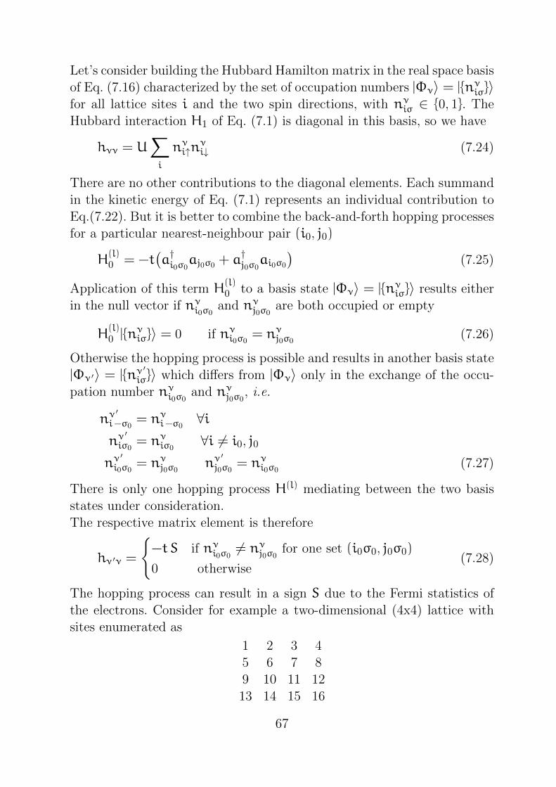
The hopping process can result in a sign S due to the Fermi statistics of

the electrons. Consider for example a two-dimensional (4x4) lattice with

sites enumerated as

1 2 3 4

5 6 7 8

9 10 11 12

13 14 15 16

67

(The numbering of sites is arbitrary but must be kept fixed.)

Now we consider hopping between sites 2 and 6 of one spin species The state

|Φν〉 be given by {niσ} = {0, 0, 1, 1, 1, 1, 0, 0, 0, 0, 0, 0, 0, 0, 0, 0} (we sup-

press the spin indices from now on). The state reads according to Eq. (7.16)

|Φν〉 = a†3a†4a†5a†6|0〉 (7.29)

Application of the hopping operator

H(l)0 = −t

(a†2a6 + a

†6a2

)(7.30)

results in the state

|Φν ′〉 = a†3a†4a†5a†2|0〉 = −a†2a†3a†4a†5|0〉 (7.31)

Thus, the new state is given by

|Φν ′〉 = −{0, 1, 1, 1, 1, 0, 0, 0, 0, 0, 0, 0, 0, 0, 0, 0} (7.32)

The hopping operator has shifted a bit and created a fermionic phase fac-

tor. For periodic boundary conditions, care must be taken of possible minus

signs whenever an electron is wrapped around the boundary and the num-

ber of electrons it commutes through is odd. The sign is given by

S = (−1)∆n (7.33)

where ∆n is the number of electrons at the lattice sites between the site

i0 and j0, in the example ∆n = 3.

Now that we know how the individual terms of the Hamiltonian H(l) couple

a basis state {nνiσ} represented by a bit pattern to another basis state {nν′iσ}

or to its integer representation (Iν′↑ I

ν ′↓ ).

It is still necessary to find the index ν ′ of the basis state. As they have

been generated in increasing order of their integer representation, we can

apply a bisection search to find the index. This is important if we compare

the computational cost O(L) steps of a brute force search to O(log2 L)operations of the bisection search. For example, for L = 108 there is a

factor of 106 between the two methods.

7.3 The Lanczos method

In the previous section, exact diagonalization was introduced as a method

to solve manybody Hamiltonians by calculating the Hamiltonian matrix

68

in a basis and diagonalizing it. But the corresponding matrices are of the

order (108 × 108) or larger and cannot be treated by Householder tridiag-

onalization.

The Lanczos (pronounced ["la:ntsoS]) method avoids the problem of cal-

culating and saving huge matrices in the computer memory by constructing

a basis that directly leads to a tridiagonal matrix. It is an example of a

family of projection techniques known as Krylov subspace methods.

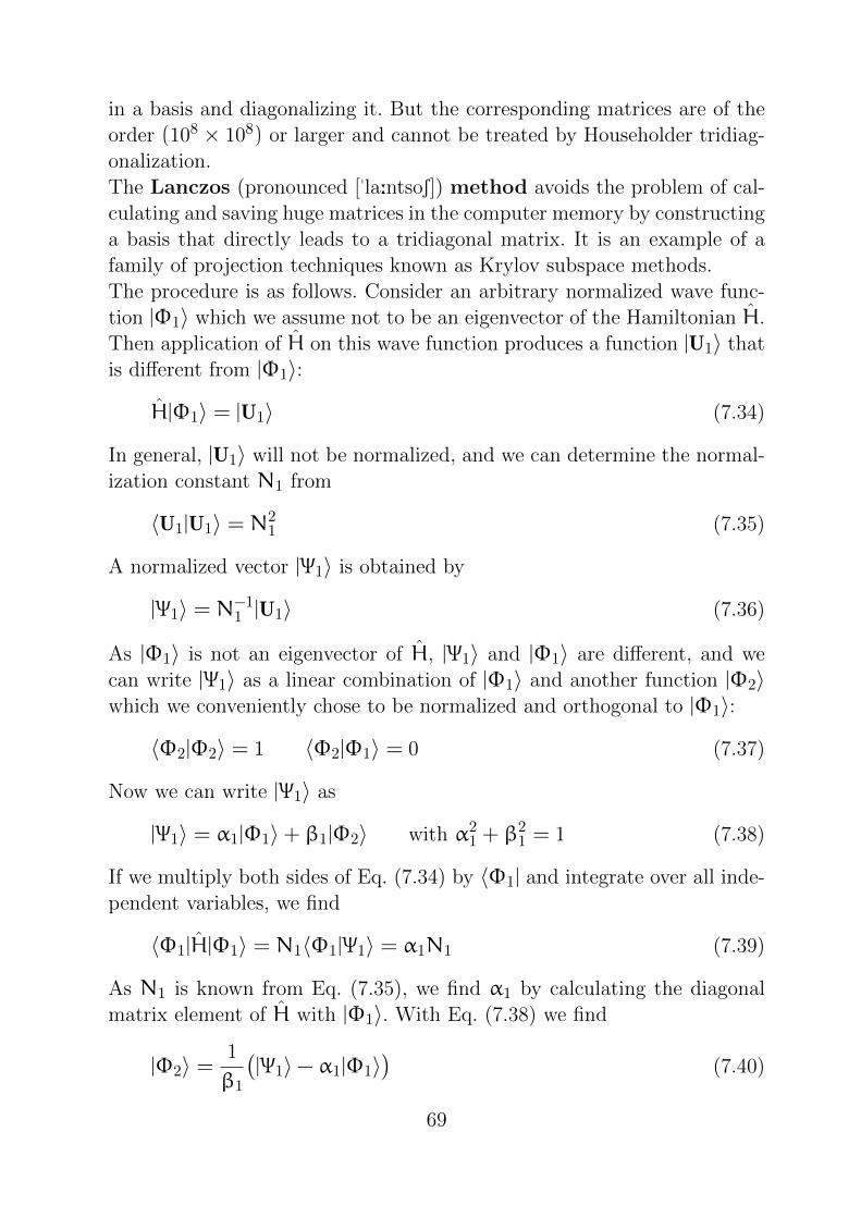
The procedure is as follows. Consider an arbitrary normalized wave func-

tion |Φ1〉 which we assume not to be an eigenvector of the Hamiltonian H.

Then application of H on this wave function produces a function |U1〉 that

is different from |Φ1〉:

H|Φ1〉 = |U1〉 (7.34)

In general, |U1〉 will not be normalized, and we can determine the normal-

ization constant N1 from

〈U1|U1〉 = N21 (7.35)

A normalized vector |Ψ1〉 is obtained by

|Ψ1〉 = N−11 |U1〉 (7.36)

As |Φ1〉 is not an eigenvector of H, |Ψ1〉 and |Φ1〉 are different, and we

can write |Ψ1〉 as a linear combination of |Φ1〉 and another function |Φ2〉which we conveniently chose to be normalized and orthogonal to |Φ1〉:

〈Φ2|Φ2〉 = 1 〈Φ2|Φ1〉 = 0 (7.37)

Now we can write |Ψ1〉 as

|Ψ1〉 = α1|Φ1〉+ β1|Φ2〉 with α21 + β

21 = 1 (7.38)

If we multiply both sides of Eq. (7.34) by 〈Φ1| and integrate over all inde-

pendent variables, we find

〈Φ1|H|Φ1〉 = N1〈Φ1|Ψ1〉 = α1N1 (7.39)

As N1 is known from Eq. (7.35), we find α1 by calculating the diagonal

matrix element of H with |Φ1〉. With Eq. (7.38) we find

|Φ2〉 =1

β1

(|Ψ1〉− α1|Φ1〉

)(7.40)

69

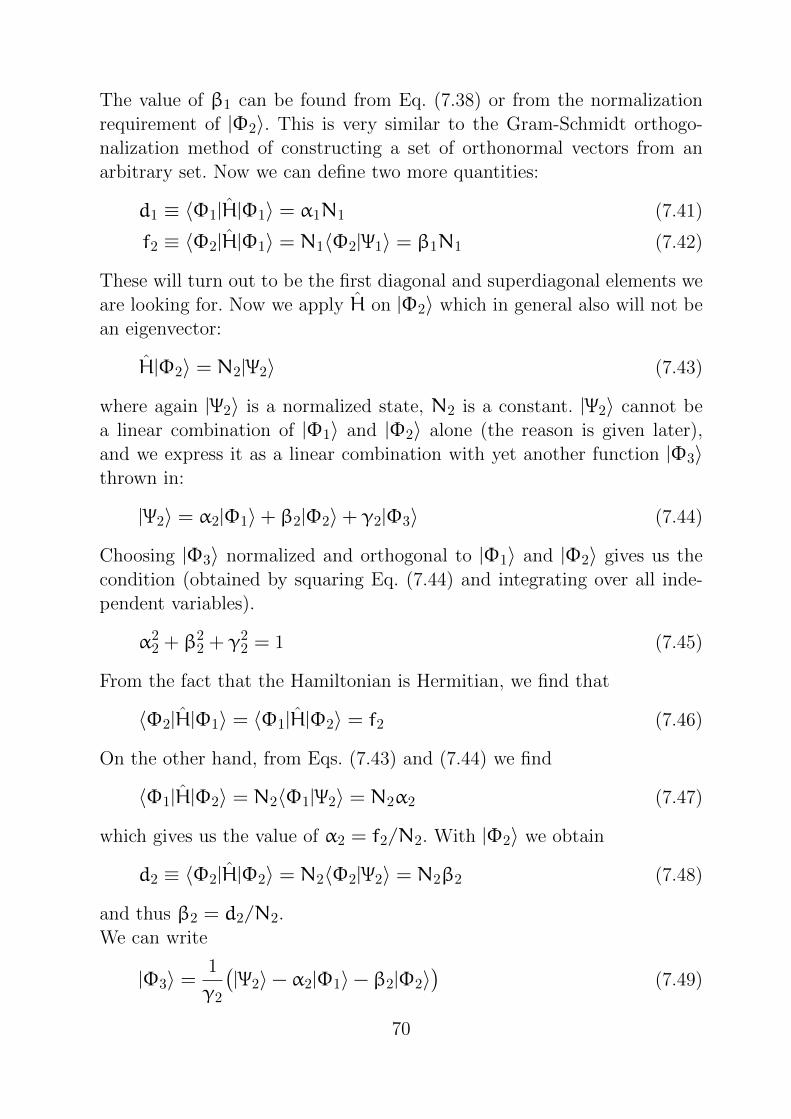
The value of β1 can be found from Eq. (7.38) or from the normalization

requirement of |Φ2〉. This is very similar to the Gram-Schmidt orthogo-

nalization method of constructing a set of orthonormal vectors from an

arbitrary set. Now we can define two more quantities:

d1 ≡ 〈Φ1|H|Φ1〉 = α1N1 (7.41)

f2 ≡ 〈Φ2|H|Φ1〉 = N1〈Φ2|Ψ1〉 = β1N1 (7.42)

These will turn out to be the first diagonal and superdiagonal elements we

are looking for. Now we apply H on |Φ2〉 which in general also will not be

an eigenvector:

H|Φ2〉 = N2|Ψ2〉 (7.43)

where again |Ψ2〉 is a normalized state, N2 is a constant. |Ψ2〉 cannot be

a linear combination of |Φ1〉 and |Φ2〉 alone (the reason is given later),

and we express it as a linear combination with yet another function |Φ3〉thrown in:

|Ψ2〉 = α2|Φ1〉+ β2|Φ2〉+ γ2|Φ3〉 (7.44)

Choosing |Φ3〉 normalized and orthogonal to |Φ1〉 and |Φ2〉 gives us the

condition (obtained by squaring Eq. (7.44) and integrating over all inde-

pendent variables).

α22 + β

22 + γ

22 = 1 (7.45)

From the fact that the Hamiltonian is Hermitian, we find that

〈Φ2|H|Φ1〉 = 〈Φ1|H|Φ2〉 = f2 (7.46)

On the other hand, from Eqs. (7.43) and (7.44) we find

〈Φ1|H|Φ2〉 = N2〈Φ1|Ψ2〉 = N2α2 (7.47)

which gives us the value of α2 = f2/N2. With |Φ2〉 we obtain

d2 ≡ 〈Φ2|H|Φ2〉 = N2〈Φ2|Ψ2〉 = N2β2 (7.48)

and thus β2 = d2/N2.

We can write

|Φ3〉 =1

γ2

(|Ψ2〉− α2|Φ1〉− β2|Φ2〉

)(7.49)

70

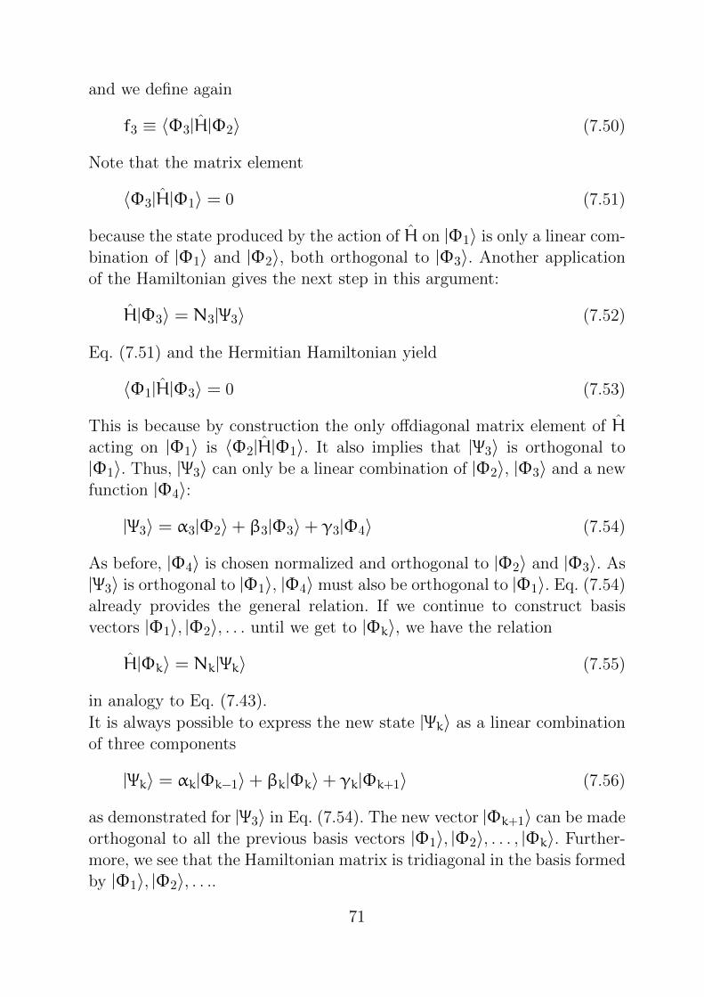
and we define again

f3 ≡ 〈Φ3|H|Φ2〉 (7.50)

Note that the matrix element

〈Φ3|H|Φ1〉 = 0 (7.51)

because the state produced by the action of H on |Φ1〉 is only a linear com-

bination of |Φ1〉 and |Φ2〉, both orthogonal to |Φ3〉. Another application

of the Hamiltonian gives the next step in this argument:

H|Φ3〉 = N3|Ψ3〉 (7.52)

Eq. (7.51) and the Hermitian Hamiltonian yield

〈Φ1|H|Φ3〉 = 0 (7.53)

This is because by construction the only offdiagonal matrix element of Hacting on |Φ1〉 is 〈Φ2|H|Φ1〉. It also implies that |Ψ3〉 is orthogonal to

|Φ1〉. Thus, |Ψ3〉 can only be a linear combination of |Φ2〉, |Φ3〉 and a new

function |Φ4〉:

|Ψ3〉 = α3|Φ2〉+ β3|Φ3〉+ γ3|Φ4〉 (7.54)

As before, |Φ4〉 is chosen normalized and orthogonal to |Φ2〉 and |Φ3〉. As

|Ψ3〉 is orthogonal to |Φ1〉, |Φ4〉 must also be orthogonal to |Φ1〉. Eq. (7.54)

already provides the general relation. If we continue to construct basis

vectors |Φ1〉, |Φ2〉, . . . until we get to |Φk〉, we have the relation

H|Φk〉 = Nk|Ψk〉 (7.55)

in analogy to Eq. (7.43).

It is always possible to express the new state |Ψk〉 as a linear combination

of three components

|Ψk〉 = αk|Φk−1〉+ βk|Φk〉+ γk|Φk+1〉 (7.56)

as demonstrated for |Ψ3〉 in Eq. (7.54). The new vector |Φk+1〉 can be made

orthogonal to all the previous basis vectors |Φ1〉, |Φ2〉, . . . , |Φk〉. Further-

more, we see that the Hamiltonian matrix is tridiagonal in the basis formed

by |Φ1〉, |Φ2〉, . . ..

71

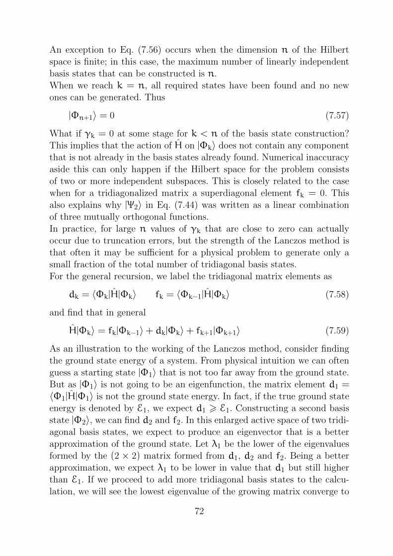
An exception to Eq. (7.56) occurs when the dimension n of the Hilbert

space is finite; in this case, the maximum number of linearly independent

basis states that can be constructed is n.

When we reach k = n, all required states have been found and no new

ones can be generated. Thus

|Φn+1〉 = 0 (7.57)

What if γk = 0 at some stage for k < n of the basis state construction?

This implies that the action of H on |Φk〉 does not contain any component

that is not already in the basis states already found. Numerical inaccuracy

aside this can only happen if the Hilbert space for the problem consists

of two or more independent subspaces. This is closely related to the case

when for a tridiagonalized matrix a superdiagonal element fk = 0. This

also explains why |Ψ2〉 in Eq. (7.44) was written as a linear combination

of three mutually orthogonal functions.

In practice, for large n values of γk that are close to zero can actually

occur due to truncation errors, but the strength of the Lanczos method is

that often it may be sufficient for a physical problem to generate only a

small fraction of the total number of tridiagonal basis states.

For the general recursion, we label the tridiagonal matrix elements as

dk = 〈Φk|H|Φk〉 fk = 〈Φk−1|H|Φk〉 (7.58)

and find that in general

H|Φk〉 = fk|Φk−1〉+ dk|Φk〉+ fk+1|Φk+1〉 (7.59)

As an illustration to the working of the Lanczos method, consider finding

the ground state energy of a system. From physical intuition we can often

guess a starting state |Φ1〉 that is not too far away from the ground state.

But as |Φ1〉 is not going to be an eigenfunction, the matrix element d1 =〈Φ1|H|Φ1〉 is not the ground state energy. In fact, if the true ground state

energy is denoted by E1, we expect d1 > E1. Constructing a second basis

state |Φ2〉, we can find d2 and f2. In this enlarged active space of two tridi-

agonal basis states, we expect to produce an eigenvector that is a better

approximation of the ground state. Let λ1 be the lower of the eigenvalues

formed by the (2 × 2) matrix formed from d1, d2 and f2. Being a better

approximation, we expect λ1 to be lower in value that d1 but still higher

than E1. If we proceed to add more tridiagonal basis states to the calcu-

lation, we will see the lowest eigenvalue of the growing matrix converge to

72

the ground state. As in many physical problems this convergence is fast,

an active space that is only a small fraction of the complete Hilbert space

is sufficient to obtain the ground state energy.

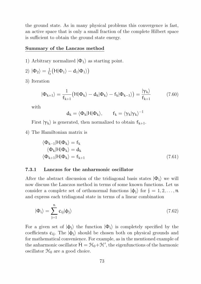
Summary of the Lanczos method

1) Arbitrary normalized |Φ1〉 as starting point.

2) |Φ2〉 = 1f2

(H|Φ1〉− d1|Φ1〉

)

3) Iteration

|Φk+1〉 =1

fk+1

(H|Φk〉− dk|Φk〉− fk|Φk−1〉

)=

|γk〉fk+1

(7.60)

with

dk = 〈Φk|H|Φk〉, fk = 〈γk|γk〉−1

First |γk〉 is generated, then normalized to obtain fk+1.

4) The Hamiltonian matrix is

〈Φk−1|H|Φk〉 = fk〈Φk|H|Φk〉 = dk〈Φk+1|H|Φk〉 = fk+1 (7.61)

7.3.1 Lanczos for the anharmonic oscillator

After the abstract discussion of the tridiagonal basis states |Φi〉 we will

now discuss the Lanczos method in terms of some known functions. Let us

consider a complete set of orthonormal functions |φj〉 for j = 1, 2, . . . ,nand express each tridiagonal state in terms of a linear combination

|Φi〉 =n∑

j=1

cij|φj〉 (7.62)

For a given set of |φj〉 the function |Φi〉 is completely specified by the

coefficients cij. The |φj〉 should be chosen both on physical grounds and

for mathematical convenience. For example, as in the mentioned example of

the anharmonic oscillator H = H0+H ′, the eigenfunctions of the harmonic

oscillator H0 are a good choice.

73

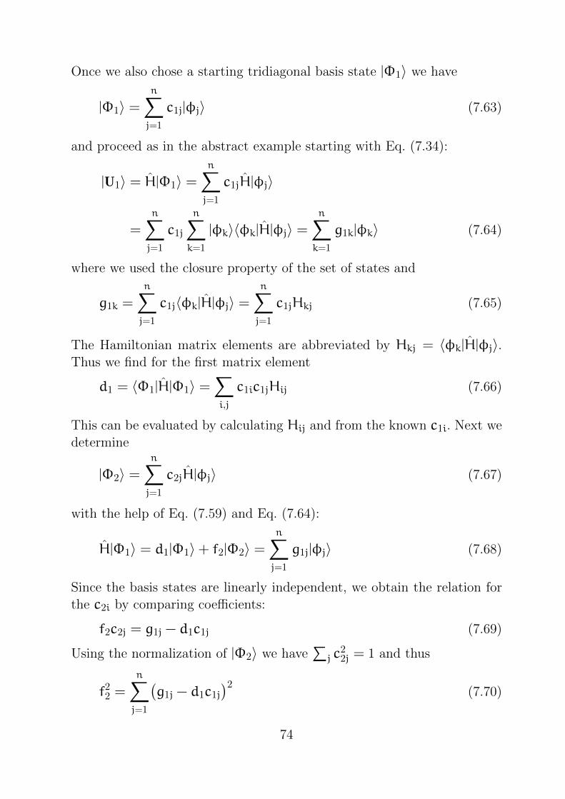
Once we also chose a starting tridiagonal basis state |Φ1〉 we have

|Φ1〉 =n∑

j=1

c1j|φj〉 (7.63)

and proceed as in the abstract example starting with Eq. (7.34):

|U1〉 = H|Φ1〉 =n∑

j=1

c1jH|φj〉

=

n∑

j=1

c1j

n∑

k=1

|φk〉〈φk|H|φj〉 =n∑

k=1

g1k|φk〉 (7.64)

where we used the closure property of the set of states and

g1k =

n∑

j=1

c1j〈φk|H|φj〉 =n∑

j=1

c1jHkj (7.65)

The Hamiltonian matrix elements are abbreviated by Hkj = 〈φk|H|φj〉.Thus we find for the first matrix element

d1 = 〈Φ1|H|Φ1〉 =∑

i,j

c1ic1jHij (7.66)

This can be evaluated by calculating Hij and from the known c1i. Next we

determine

|Φ2〉 =n∑

j=1

c2jH|φj〉 (7.67)

with the help of Eq. (7.59) and Eq. (7.64):

H|Φ1〉 = d1|Φ1〉+ f2|Φ2〉 =n∑

j=1

g1j|φj〉 (7.68)

Since the basis states are linearly independent, we obtain the relation for

the c2i by comparing coefficients:

f2c2j = g1j − d1c1j (7.69)

Using the normalization of |Φ2〉 we have∑j c

22j = 1 and thus

f22 =

n∑

j=1

(g1j − d1c1j

)2(7.70)

74

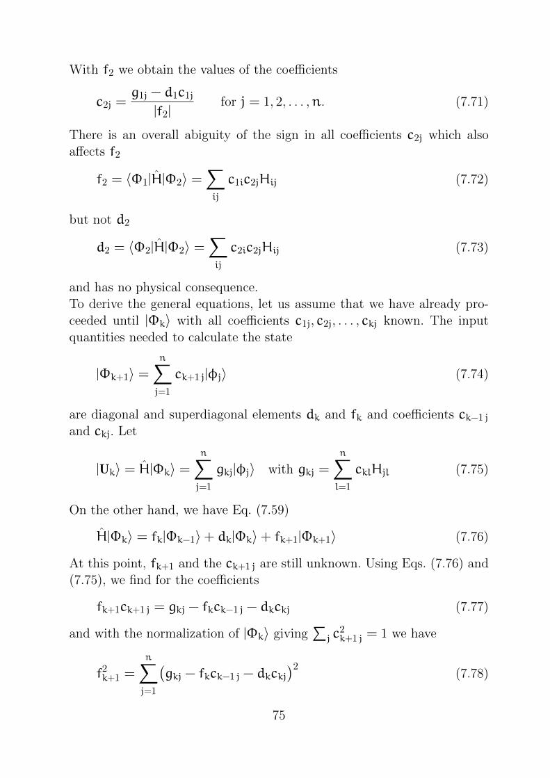
With f2 we obtain the values of the coefficients

c2j =g1j − d1c1j

|f2|for j = 1, 2, . . . ,n. (7.71)

There is an overall abiguity of the sign in all coefficients c2j which also

affects f2

f2 = 〈Φ1|H|Φ2〉 =∑

ij

c1ic2jHij (7.72)

but not d2

d2 = 〈Φ2|H|Φ2〉 =∑

ij

c2ic2jHij (7.73)

and has no physical consequence.

To derive the general equations, let us assume that we have already pro-

ceeded until |Φk〉 with all coefficients c1j, c2j, . . . , ckj known. The input

quantities needed to calculate the state

|Φk+1〉 =n∑

j=1

ck+1 j|φj〉 (7.74)

are diagonal and superdiagonal elements dk and fk and coefficients ck−1 j

and ckj. Let

|Uk〉 = H|Φk〉 =n∑

j=1

gkj|φj〉 with gkj =

n∑

l=1

cklHjl (7.75)

On the other hand, we have Eq. (7.59)

H|Φk〉 = fk|Φk−1〉+ dk|Φk〉+ fk+1|Φk+1〉 (7.76)

At this point, fk+1 and the ck+1 j are still unknown. Using Eqs. (7.76) and

(7.75), we find for the coefficients

fk+1ck+1 j = gkj − fkck−1 j − dkckj (7.77)

and with the normalization of |Φk〉 giving∑j c

2k+1 j = 1 we have

f2k+1 =

n∑

j=1

(gkj − fkck−1 j − dkckj

)2(7.78)

75

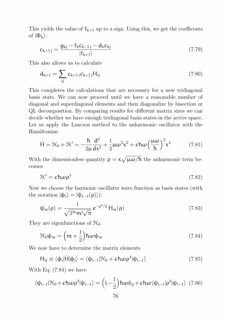
This yields the value of fk+1 up to a sign. Using this, we get the coefficents

of |Φk〉:

ck+1 j =gkj − fkck−1 j − dkckj

|fk+1|(7.79)

This also allows us to calculate

dk+1 =∑

ij

ck+1 ick+1 jHij (7.80)

This completes the calculations that are necessary for a new tridiagonal

basis state. We can now proceed until we have a reasonable number of

diagonal and superdiagonal elements and then diagonalize by bisection or

QL decomposition. By comparing results for different matrix sizes we can

decide whether we have enough tridiagonal basis states in the active space.

Let us apply the Lanczos method to the anharmonic oscillator with the

Hamiltonian

H = H0 +H ′ = − h

2µ

d2

dx2+

1

2µω2x2 + ε hω

(µω h

)2x4 (7.81)

With the dimensionless quantity ρ = x√µω/ h the anharmonic term be-

comes

H ′ = ε hωρ4 (7.82)

Now we choose the harmonic oscillater wave function as basis states (with

the notation |φi〉 = |ψi−1(ρ)〉):

ψm(ρ) =1√

2mm!√πe−ρ

2/2 Hm(ρ) (7.83)

They are eigenfunctions of H0:

H0ψm =(m+

1

2

) hωψm (7.84)

We now have to determine the matrix elements

Hij ≡ 〈φi|H|φj〉 = 〈ψi−1|H0 + ε hωρ4|ψi−1〉 (7.85)

With Eq. (7.84) we have

〈ψi−1|H0+ε hωρ4|ψi−1〉 =

(i−

1

2

) hωδij+ε hω〈ψi−1|ρ

4|ψi−1〉 (7.86)

76

For m = min(i, j) − 1 the matrix elements of ρ4 are

〈ψi−1|ρ4|ψi−1〉 =

32

(m2 +m+ 1

2

)for i = j(

m+ 32

)√(m+ 1)(m+ 2) for i = j± 2

14

√(m+ 1)(m+ 2)(m+ 3)(m+ 4) for i = j± 4

0 otherwise

(7.87)

A reasonable starting point for constructing the tridiagonal basis states is

the ground state of the harmonic oscillator:

|Φ1〉 = |φ1〉 ≡ |ψ0(ρ)〉 (7.88)

This corresponds to the coefficients

c1j =

{1 for j = 1

0 otherwise(7.89)

The first diagonal matrix element in the tridiagonal basis is then

d1 = 〈Φ1|H|Φ1〉 = 〈ψ0|H0 + ε hωρ4|ψ0〉 =

(1

2+

3ε

4

) hω (7.90)

To obtain |Φ2〉 we use Eq. (7.64) to obtain

g1k =

n∑

j=1

c1jHkj = Hk1 =

d1 for k = 13√2 hωε for k = 3√32 hωε for k = 5

0 otherwise

(7.91)

From these we get

f22 = h2ω2ε2(9

2+

3

2

)= 6 h2ω2ε2 (7.92)

and the values of the coefficients c2j

c2j ={

0, 0,

√3

2, 0,

1

2, 0, 0, . . . , 0

}(7.93)

The rest of the calculations can be carried out iteratively. For k > 2 we

can calculate dk from

dk =∑

ij

= ckickjHij (7.94)

77

and the fk can be obtained from Eq. (7.78). For each k > 2 the calculations

proceeds in the order fk, ckj,dk,gkj.

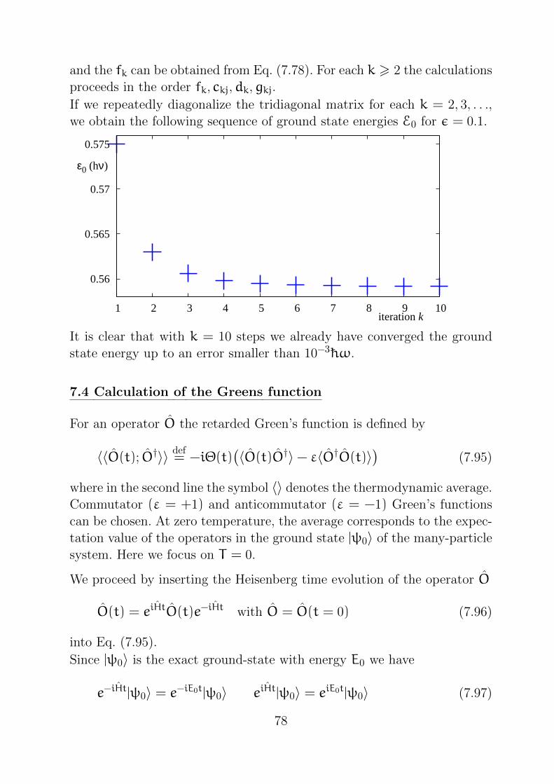
If we repeatedly diagonalize the tridiagonal matrix for each k = 2, 3, . . .,

we obtain the following sequence of ground state energies E0 for ε = 0.1.

0.56

0.565

0.57

0.575

1 2 3 4 5 6 7 8 9 10

ε0 (hν)

iteration k

It is clear that with k = 10 steps we already have converged the ground

state energy up to an error smaller than 10−3 hω.

7.4 Calculation of the Greens function

For an operator O the retarded Green’s function is defined by

〈〈O(t); O†〉〉 def= −iΘ(t)

(〈O(t)O†〉− ε〈O†O(t)〉

)(7.95)

where in the second line the symbol 〈〉 denotes the thermodynamic average.

Commutator (ε = +1) and anticommutator (ε = −1) Green’s functions

can be chosen. At zero temperature, the average corresponds to the expec-

tation value of the operators in the ground state |ψ0〉 of the many-particle

system. Here we focus on T = 0.

We proceed by inserting the Heisenberg time evolution of the operator O

O(t) = eiHtO(t)e−iHt with O = O(t = 0) (7.96)

into Eq. (7.95).

Since |ψ0〉 is the exact ground-state with energy E0 we have

e−iHt|ψ0〉 = e−iE0t|ψ0〉 eiHt|ψ0〉 = eiE0t|ψ0〉 (7.97)

78

and with ω+ = ω + iδ, where δ is an infinitesimal positive quantity, we

obtain

〈〈O; O†〉〉ωdef=

∫∞

−∞dt eiω

+t〈〈O(t); O†〉〉

= −i

∫∞

0dt eiω

+t(〈eiHtOe−iHtO†〉− ε〈O†eiHtOe−iHt〉

)

= −i

∫∞

0dt eiω

+t(〈Oe−i(H−E0)tO†〉− ε〈O†ei(H−E0)tO〉

)

= −i(⟨O

∫∞

0dt ei(ω

+−H+E0)tO†⟩− ε⟨O†∫∞

0dt ei(ω

++H−E0)tO⟩)

(7.98)

With the aid of the spectral theorem the integral can be evaluated. Now,

taking into account that we perform the average in the ground state |ψ0〉,we obtain

〈〈O; O†〉〉ω =⟨O

1

ω+ − (H− E0)O†⟩− ε⟨O†

1

ω+ + (H− E0)O⟩

= 〈ψ0|OO†|ψ0〉

⟨φ0

∣∣∣ 1

ω+ − (H− E0)

∣∣∣φ0

⟩

− ε〈ψ0|O†O|ψ0〉

⟨φ0

∣∣∣ 1

ω+ + (H− E0)

∣∣∣φ0

⟩(7.99)

The normalized state vectors φ0 and φ0, defined by

|φ0〉 =O†|ψ0〉√〈ψ0|OO†|ψ0〉

|φ0〉 =O|ψ0〉√〈ψ0|O†O|ψ0〉

(7.100)

are used as initial vectors for two independent Lanczos sequences.

The tridiagonal form of H, and likewise of the energy denominators H =ω ± (H − E0) in the Lanczos basis can be exploited to determine the

expectation value of the inverse of H = ω± (H−E0) in Eq. (7.99). As for

the ground state we calculate the matrix elements for the Lanczos vectors

〈φi|H− E0|φi〉 = ∆εi〈φi|H− E0|φi+1〉 = ki〈φi|H− E0|φj〉 = 0 ∀|i− j| > 1 (7.101)

79

Together with the orthonormality

〈φi|φj〉 = δij (7.102)

we obtain the tridiagonal form

(ω+ ± (H− E0))

=

ω+ ± ∆ε0 k1

k1 ω+ ± ∆ε1 k2

k2 ω+ ± ∆ε2 k3

k3 ω+ ± ∆ε3 k4

k4. . .

(7.103)

We need the (0, 0) element of the inverse.

The (i, j) element of an inverse matrix can be expressed by

(A−1)ij = (−1)i+jdet∆ij

detA(7.104)

where ∆ij denotes the submatrix of A obtained by eliminating from A the

ith row and the jth column. Especially for the desired (0, 0) element of the

inverse we have

(A−1)00 =det∆00

detA(7.105)

Because of the tridiagonal structure of the above matrix, the formula sim-

plifies as follows. Consider the matrix

A =

A00 A01

A10 A11 A12

A21 A22 A23

A32 A33 A34

A43 A44

(7.106)

The determinant can be expanded along the first row and column:

detA = A00det

A11 A12

A21 A22 A23

A32 A33 A34

A43 A44

−A01A10det

A22 A23

A32 A33 A34

A43 A44

(7.107)

80

We define the determinant of the submatrix of A beginning with the ithcolumn and row, i.e.

Didef= det

Ai i Ai i+1

Ai+1 i Ai+1 i+1 Ai+1 i+2

Ai+2 i+1 Ai+2 i+2 Ai+2 i+3

Ai+3 i+2 Ai+3 i+3

(7.108)

Then, we can write the desired element of the inverse matrix (7.105) as

(A−1)00 =1D0D1

(7.109)

We can now use Eq. (7.107) to express D0/D1 by D1/D2:

D0

D1=A00D1 − |A01|

2D2

D1= A00 −

|A01|2

D1D2

(7.110)

Iterating the above reasoning yields

Dl

Dl+1= Al l −

|Al l+1|2

Dl+1

Dl+2

(7.111)

This leads to a continued fraction for the desired quantity

(A−1)00 =1D0D1

=1

A00 −|A01|

2

A11 −|A12|

2

A22 −|A23|

2

A33 −. . .

(7.112)

For the original problem((ω+ ± (H − E0))

−1)

00the continued fraction

reads((ω+ ± (H− E0))

−1)

00

=1

ω+ ± ∆ε0 −|k1|

2

ω+ ± ∆ε1 −|k2|

2

ω+ ± ∆ε2 −|k3|

2

ω+ ± ∆ε3 −. . .

(7.113)

81

This expression is well suited for numerical treatment and can be iterated

for arbitrary ω. To this end, we introduce the abbreviations

di = ω+ ± ∆εi for i = 0, 1, . . .

ei = |ki|2 for i = 1, 2, . . . (7.114)

Beginning with the upper left (2×2) submatrix of A the continued fraction

has the form

1

d0 −e1

d1 − R1

=d1 − R1

d0d1 − d1 − d0R1≡ a1 + a0R1

b1 + b0R1(7.115)

In this equation we anticipated the general form. The remainder R1 has

again the form of a continued fraction. In general the remainder reads

Ri =ei+1

di+1 − Ri+1(7.116)

By substituting this for i = 1 into Eq. (7.115) we obtain

a1 a0

a1 + a0R1

b1 + b0R1=

︷ ︸︸ ︷a1d1 + a0e2 +

︷ ︸︸ ︷(−a1)R2

b1d2 + b0e2︸ ︷︷ ︸+(−b1)︸ ︷︷ ︸R2

b1 b0 (7.117)

which is again of the form

a1 + a0R

b1 + b0R(7.118)

Thus the iteration formula for i = 1, 2, . . . deduced from the considerations

above is given by

a1 −→ a1di+1 + a0ei+1

a0 −→ −a1

b1 −→ b1di+1 + b0ei+1

b0 −→ −b1 (7.119)

with the initial values a1 = d1, a0 = −1, b1 = d0d1 − e1, b0 = −d0. The

sequence is iterated for each ω individually and ends if the Krylov space

is exhausted or if a desired convergence of

g(ω) =a1

b1(7.120)

82

is achieved. In order to avoid numerical instabilities, it is recommended to

rescale all quantities a0,a1,b0,b1 e.g. by b1 after each iteration.

In some cases it may happen that the Green’s function of interest is not

diagonal in the operators, e.g.

gAB =⟨A†

1

ω+ − (H− E0)B⟩

(7.121)

In this case we define two operators Oα = A + αB and determine the

diagonal Green’s functions

gα =⟨O†α

1

ω+ − (H− E0)Oα

⟩(7.122)

It is easily possible to separate gAB by linearly combining the four Green’s

functions for α = {±1,±i}.

Lehmann Representation

There is an alternative way of calculating Green’s functions, the so-called

Lehmann representation. Again we consider the matrix elements of the

form⟨ψ0

∣∣∣O† 1

ω+ ± (H− E0)O∣∣∣ψ0

⟩(7.123)

where |ψ0〉 represents the ground state. Like before we define |φ0〉 as the

normalized vector O|ψ0〉, which serves as initial vector of a Lanczos se-

quence. We insert a complete orthonormal set of eigenvectors of H given

by

1I =∑

ν

|ψν〉〈ψν| (7.124)

Then Eq. (7.123) can be cast into the form

⟨ψ0

∣∣∣O† 1

ω+ ± (H− E0)O∣∣∣ψ0

⟩=∑

ν

〈ψ0|O†|ψν〉〈ψν|O|ψ0〉

ω+ ± (H− E0)(7.125)

Next we expand the eigenvectors |ψν〉 in the Lanczos basis {|φi〉}

|ψν〉 =∑

i

c(ν)i |φi〉 with c

(ν)i = 〈φi|ψν〉 (7.126)

83

to obtain

〈ψν|O|ψ0〉 =∑

i

c(ν)∗i 〈φi|O|ψ0〉 =

√〈ψ0|O†O|ψ0〉

∑

i

c(ν)∗i 〈φi|φ0〉

=

√〈ψ0|O†O|ψ0〉c(ν)∗i

(7.127)

because 〈φi|φ0〉 = δi0. This means that except of the first terms all ad-

dends vanish.

Thus Eq. (7.123) can be approximated by

⟨ψ0

∣∣∣O† 1

ω+ ± (H− E0)O∣∣∣ψ0

⟩= 〈ψ0|O

†O|ψ0〉NL∑

ν=1

|c(ν)0 |2

ω+ ± (E− E0)

(7.128)

where only the first components c(ν)0 of the expansion of the eigenvector

|ψν〉 in the Lanczos basis are required. In general, the eigenstates |ψν〉(ν =1, . . . ,NL), computed by the Lanczos procedure, do not form a complete

set of basis vectors, nor are the respective energies Eν exact eigenvalues of

H. However, with increasing number of iterations, the Lanczos procedure

converges towards the exact Green’s function and the convergence can be

monitored and stopped as soon as the desired accuracy is reached. The

approximate Lehmann representation (7.128) is an explicit sum of simple

poles. The same is true for the continued fraction.

84