Embed Size (px)
Citation preview
Chapter 4 Potential Earth Science Hazards (PESH)
Potential earth science hazards (PESH) include ground motion, ground failure (i.e., liquefaction, landslide and surface fault rupture) and tsunami/seiche. Methods for developing estimates of ground motion and ground failure are discussed in the following sections. Tsunami/seiche can be included in the Methodology in the form of user-supplied inundation maps as discussed in Chapter 9. The Methodology, highlighting the PESH component, is shown in Flowchart 4.1.
4.1 Ground Motion
4.1.1 Introduction
Ground motion estimates are generated in the form of GIS-based contour maps and location-specific seismic demands stored in relational databases. Ground motion is characterized by: (1) spectral response, based on a standard spectrum shape, (2) peak ground acceleration and (3) peak ground velocity. The spatial distribution of ground motion can be determined using one of the following methods or sources:
• Deterministic ground motion analysis (Methodology calculation) • USGS probabilistic ground motion maps (maps supplied with HAZUS) • Other probabilistic or deterministic ground motion maps (user-supplied maps)
Deterministic seismic ground motion demands are calculated for user-specified scenario earthquakes (Section 4.1.2.1). For a given event magnitude, attenuation relationships (Section 4.1.2.3) are used to calculate ground shaking demand for rock sites (Site Class B), which is then amplified by factors (Section 4.1.2.4) based on local soil conditions when a soil map is supplied by the user. The attenuation relationships provided with the Methodology for Western United States (WUS) sites are based on Boore, Joyner & Fumal (1993, 1994a, 1994b), Campbell and Bozorgnia (1994), Munson and Thurber (1997), Sadigh, Chang, Abrahamson, Chiou and Power (1993) and Youngs, Chiou, Silva and Humphrey (1997). For sites in the Central and Eastern United States (CEUS), the attenuation relationships are based on Frankel et al. (1996), Savy (1998) and Toro, Abrahamson and Schneider (1997).
In the Methodology’s probabilistic analysis procedure, the ground shaking demand is characterized by spectral contour maps developed by the United States Geological Survey (USGS) as part of Project 97 project (Frankel et. al, 1996). The Methodology includes maps for eight probabilistic hazard levels: ranging from ground shaking with a 39% probability of being exceeded in 50 years (100 year return period) to the ground shaking with a 2% probability of being exceeded in 50 years (2500 year return period). The USGS maps describe ground shaking demand for rock (Site Class B) sites, which the Methodology amplifies based on local soil conditions.
HAZUS99-SR2 Technical Manual 4-1

Chapter 4. Potential Earth Science Hazards (PESH)
8. Utility
Systems
4. Ground Motion 4. Ground Failure
Direct Physical Damage
6. Essential and High Potential Loss Facilities
12. Debris10. Fire 15. Economic14. Shelter9. Inundation 11. HazMat
16. Indirect Economic
Losses
Potential Earth Science Hazards
Direct Economic/ Social Losses
Induced Physical Damage
7. Transportation
Systems
5. General Building
Stock
13. Casualities
Lifelines-Lifelines-
Flowchart 4.1: Ground Motion and Ground Failure Relationship to other Modules of the Earthquake Loss Estimation Methodology
4-2 HAZUS99-SR2 Technical Manual
•••
•••
Chapter 4. Potential Earth Science Hazards (PESH)
User-supplied peak ground acceleration (PGA) and spectral acceleration contour maps may also be used with HAZUS (Section 4.1.2.1). In this case, the user must provide all contour maps in a pre-defined digital format (as specified in the User’s Manual). As stated in Section 4.1.2.1, the Methodology assumes that user-supplied maps include soil amplification.
4.1.1.1 Form of Ground Motion Estimates / Site Effects
Ground motion estimates are represented by: (1) contour maps and (2) location-specific values of ground shaking demand. For computational efficiency and improved accuracy, earthquake losses are generally computed using location-specific estimates of ground shaking demand. For general building stock the analysis has been simplified so that ground motion demand is computed at the centroid of a census tract. However, contour maps are also developed to provide pictorial representations of the variation in ground motion demand within the study region. When ground motion is based on either USGS or user-supplied maps, location-specific values of ground shaking demand are interpolated between PGA, PGV or spectral acceleration contours, respectively.
Elastic response spectra (5% damping) are used by the Methodology to characterize ground shaking demand. These spectra all have the same “standard” format defined by a PGA value (at zero period) and spectral response at a period of 0.3 second (acceleration domain) and spectral response at a period of 1.0 second (velocity domain). Ground shaking demand is also defined by peak ground velocity (PGV).
4.1.1.2 Input Requirements and Output Information
For computation of ground shaking demand, the following inputs are required:
• Scenario Basis - The user must select the basis for determining ground shaking demand from one of three options: (1) a deterministic calculation, (2) probabilistic maps, supplied with the Methodology, or (3) user-supplied maps. For deterministic calculation of ground shaking, the user specifies a scenario earthquake magnitude and location. In some cases, the user may also need to specify certain source attributes required by the attenuation relationships supplied with the Methodology.
• Attenuation Relationship - For deterministic calculation of ground shaking, the user selects an appropriate attenuation relationship from those supplied with the Methodology. Attenuation relationships are based on the geographic location of the study region (Western United States vs. Central Eastern United States) and on the type of fault for WUS sources. WUS regions include locations in, or west of, the Rocky Mountains, Hawaii and Alaska. Figure 4-1 shows the regional separation of WUS and CEUS locations as defined in Project 97 (Frankel et al., 1996). The designation of states as WUS or CEUS as specified in the Methodology is found in Table 3C.1. For WUS sources, the attenuation functions predict ground shaking
HAZUS99-SR2 Technical Manual 4-3

•••
Chapter 4. Potential Earth Science Hazards (PESH)
based on source type, including: (1) strike-slip faults, (2) reverse-slip faults, (3) normal faults (4) deep faults (> 50 km) and (5) Cascadia subduction zone sources. The Methodology provides “default” combinations of attenuation functions for the WUS and CEUS, respectively, following the theory developed by the USGS for the 48 contiguous states in Project 97 (Frankel et al., 1996), for Alaska (Frankel, 1997), and Hawaii (Klein et al., 1998).
WUS CEUS
Figure 4.1 Boundaries Between WUS and CEUS Locations as Defined in Project 97.
• Soil Map - The user may supply a detailed soil map to account for local site conditions. This map must identify soil type using a scheme that is based on, or can be related to, the site class definitions of the 1997 NEHRP Provisions (Section 4.1.2.4), and must be in pre-defined digital format (as specified in the User’s Manual). In the absence of a soil map, HAZUS will amplify the ground motion demand assuming Site Class D soil at all sites. However; a user may specify a soil map on a census tract basis using HAZUS (see Section 6.8 of the User’s Manual).
4.1.2 Description of Methods
The description of the methods for calculating ground shaking is divided into four separate areas: • Basis for ground shaking (Section 4.1.2.1) • Standard shape of response spectra (Section 4.1.2.2) • Attenuation of ground shaking (Section 4.1.2.3) • Amplification of ground shaking - local site conditions (Section 4.1.2.4)
4-4 HAZUS99-SR2 Technical Manual

Chapter 4. Potential Earth Science Hazards (PESH)
4.1.2.1 Basis for Ground Shaking
The methodology supports three options as the basis for ground shaking:
• Deterministic calculation of scenario earthquake ground shaking • Probabilistic seismic hazard maps (USGS) • User-supplied seismic hazard maps
Deterministic Calculation of Scenario Earthquake Ground Shaking For deterministic calculation of the scenario event, the user specifies the location (e.g., epicenter) and magnitude of the scenario earthquake. The Methodology provides three options for selection of an appropriate scenario earthquake location. The user can either: (1) specify an event based on a database of WUS seismic sources (faults), (2) specify an event based on a database of historical earthquake epicenters, or (3) specify an event based on an arbitrary choice of the epicenter. These options are described below.
Seismic Source Database (WUS Fault Map) For the WUS, the Methodology provides a database of seismic sources (fault segments) developed by the USGS, the California Department of Mines and Geology (CDMG) and the Nevada Bureau of Mines and Geology (NBMG). The user accesses the database map (using HAZUS) and selects a magnitude and epicenter on one of the identified fault segments. The database includes information on fault segment type, location, orientation and geometry (e.g., depth, width and dip angle), as well as on each fault segment’s seismic potential (e.g., maximum moment).
The Methodology computes the expected values of surface and subsurface fault rupture length. Fault rupture length is based on the relationship of Wells and Coppersmith (1994) given below:
log10 ( ) = a + b ⋅ M (4-1)L
where: L is the rupture length (km) M is the moment magnitude of the earthquake
HAZUS99-SR2 Technical Manual 4-5
Chapter 4. Potential Earth Science Hazards (PESH)
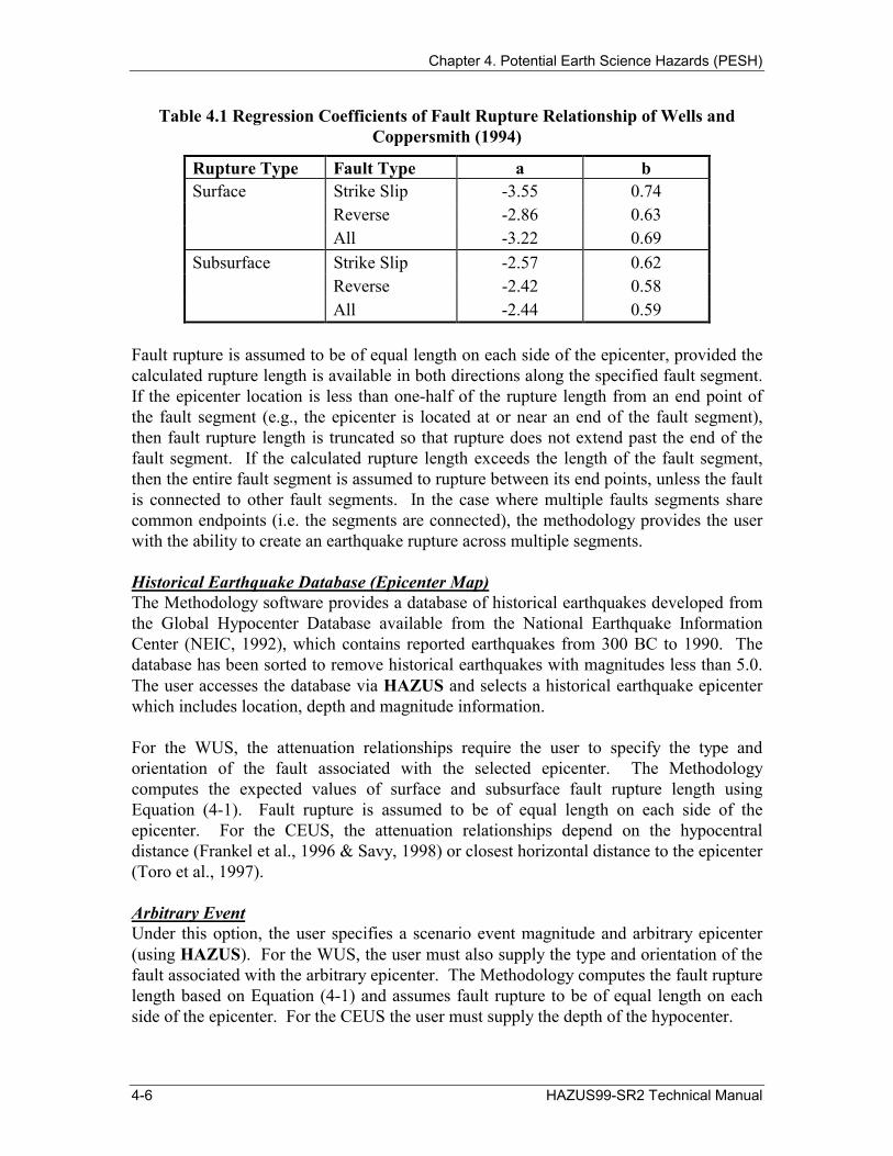
Table 4.1 Regression Coefficients of Fault Rupture Relationship of Wells and Coppersmith (1994)
Rupture Type Fault Type a b Surface Strike Slip
Reverse All
-3.55 -2.86 -3.22
0.74 0.63 0.69
Subsurface Strike Slip Reverse All
-2.57 -2.42 -2.44
0.62 0.58 0.59
Fault rupture is assumed to be of equal length on each side of the epicenter, provided the calculated rupture length is available in both directions along the specified fault segment. If the epicenter location is less than one-half of the rupture length from an end point of the fault segment (e.g., the epicenter is located at or near an end of the fault segment), then fault rupture length is truncated so that rupture does not extend past the end of the fault segment. If the calculated rupture length exceeds the length of the fault segment, then the entire fault segment is assumed to rupture between its end points, unless the fault is connected to other fault segments. In the case where multiple faults segments share common endpoints (i.e. the segments are connected), the methodology provides the user with the ability to create an earthquake rupture across multiple segments.
Historical Earthquake Database (Epicenter Map) The Methodology software provides a database of historical earthquakes developed from the Global Hypocenter Database available from the National Earthquake Information Center (NEIC, 1992), which contains reported earthquakes from 300 BC to 1990. The database has been sorted to remove historical earthquakes with magnitudes less than 5.0. The user accesses the database via HAZUS and selects a historical earthquake epicenter which includes location, depth and magnitude information.
For the WUS, the attenuation relationships require the user to specify the type and orientation of the fault associated with the selected epicenter. The Methodology computes the expected values of surface and subsurface fault rupture length using Equation (4-1). Fault rupture is assumed to be of equal length on each side of the epicenter. For the CEUS, the attenuation relationships depend on the hypocentral distance (Frankel et al., 1996 & Savy, 1998) or closest horizontal distance to the epicenter (Toro et al., 1997).
Arbitrary Event Under this option, the user specifies a scenario event magnitude and arbitrary epicenter (using HAZUS). For the WUS, the user must also supply the type and orientation of the fault associated with the arbitrary epicenter. The Methodology computes the fault rupture length based on Equation (4-1) and assumes fault rupture to be of equal length on each side of the epicenter. For the CEUS the user must supply the depth of the hypocenter.
4-6 HAZUS99-SR2 Technical Manual

Chapter 4. Potential Earth Science Hazards (PESH)
Probabilistic Seismic Hazard Maps (USGS) The Methodology includes probabilistic seismic hazard contour maps developed by the USGS for Project 97. The USGS maps provide estimates of PGA and spectral acceleration at periods of 0.3 second and 1.0 second, respectively. Ground shaking estimates are available for eight hazard levels: ranging from the ground shaking with a 39% probability of being exceeded in 50 years to ground shakeing with a 2% probability of being exceeded in 50 years. In terms of mean return periods, the hazard levels range from 100 years to 2500 years.
User-Supplied Seismic Hazard Maps The Methodology allows the user to supply PGA and spectral acceleration contour maps of ground shaking in a pre-defined digital format (as specified in the User’s Manual). This option permits the user to develop a scenario event that could not be described adequately by the available attenuation relationships, or to replicate historical earthquakes (e.g., 1994 Northridge Earthquake). The maps of PGA and spectral acceleration (periods of 0.3 and 1.0 second) must be provided. The Methodology software assumes these ground motion maps include soil amplification, thus no soil map is required.
Should only PGA contour maps be available, the user can develop the other required maps based on the spectral acceleration response factors given in Table 4.2 (WUS) and Table 4.3 (CEUS).
4.1.2.2 Standard Shape of the Response Spectra
The Methodology characterizes ground shaking using a standardized response spectrum shape, as shown in Figure 4.2. The standardized shape consists of four parts: peak ground acceleration (PGA), a region of constant spectral acceleration at periods from zero seconds to TAV (seconds), a region of constant spectral velocity at periods from TAV to TVD (seconds) and a region of constant spectral displacement for periods of TVD and beyond.
In Figure 4.2, spectral acceleration is plotted as a function of spectral displacement (rather than as a function of period). This is the format of response spectra used for evaluation of damage to buildings (Chapter 5) and essential facilities (Chapter 6). Equation (4-2) may be used to convert spectral displacement (inches), to period (seconds) for a given value of spectral acceleration (units of g), and Equation (4-3) may be used to convert spectral acceleration (units of g) to spectral displacement (inches) for a given value of period.
T = 0.32A
D
S S (4-2)
SD = 9.8 ⋅ S A ⋅T 2 (4-3)
HAZUS99-SR2 Technical Manual 4-7

Chapter 4. Potential Earth Science Hazards (PESH)
The region of constant spectral acceleration is defined by spectral acceleration at a period of 0.3 second. The constant spectral velocity region has spectral acceleration proportional to 1/T and is anchored to the spectral acceleration at a period of 1 second. The period, TAV, is based on the intersection of the region of constant spectral acceleration and constant spectral velocity (spectral acceleration proportional to 1/T). The value of TAV varies depending on the values of spectral acceleration that define these two intersecting regions. The constant spectral displacement region has spectral acceleration proportional to 1/T2 and is anchored to spectral acceleration at the period, TVD, where constant spectral velocity transitions to constant spectral displacement.
The period, TVD, is based on the reciprocal of the corner frequency, fc, which is proportional to stress drop and seismic moment. The corner frequency is estimated in Joyner and Boore (1988) as a function of moment magnitude (M). Using Joyner and Boore’s formulation, the period TVD, in seconds, is expressed in terms of the earthquake’s moment magnitude as shown by the following Equation (4-4):
(M 5)−
TVD 1/fc =10= (4-4)2
When the moment magnitude of the scenario earthquake is not known (e.g., when using USGS maps or user-supplied maps), the period TVD is assumed to be 10 seconds (i.e., moment magnitude is assumed to be M = 7.0).
Standard Shape - Site Class B
Typical Shape - Site Class B (WUS)
0.3 sec.
1.0 sec.
TAV
TVD
SA (Velocity Domain) αααα 1/T
PGA
Spec
tral
Acc
eler
atio
n (g
's)
Spectral Displacement (inches)
Figure 4.2 Standardized Response Spectrum Shape
4-8 HAZUS99-SR2 Technical Manual
Chapter 4. Potential Earth Science Hazards (PESH)
Using a standard response spectrum shape simplifies calculation of response needed in estimating damage and loss. In reality, the shape of the spectrum will vary depending on whether the earthquake occurs in the WUS or CEUS, whether it is a large or moderate size event and whether the site is near or far from the earthquake source. However, the differences between the shape of an actual spectrum and the standard spectrum tend to be significant only at periods less than 0.3 second and at periods greater than TVD, which do not significantly affect the Methodology’s estimation of damage and loss.
The standard response spectrum shape (with adjustment for site amplification) represents all site/source conditions, except for site/source conditions that have strong amplification at periods beyond 1 second. Although relatively rare, strong amplification at periods beyond 1 second can occur. For example, strong amplification at a period of about 2 seconds caused extensive damage and loss to taller buildings in parts of Mexico City during the 1985 Michoacan earthquake. In this case, the standard response spectrum shape would tend to overestimate short-period spectral acceleration and to underestimate long-period (i.e., greater than 1-second) spectral acceleration.
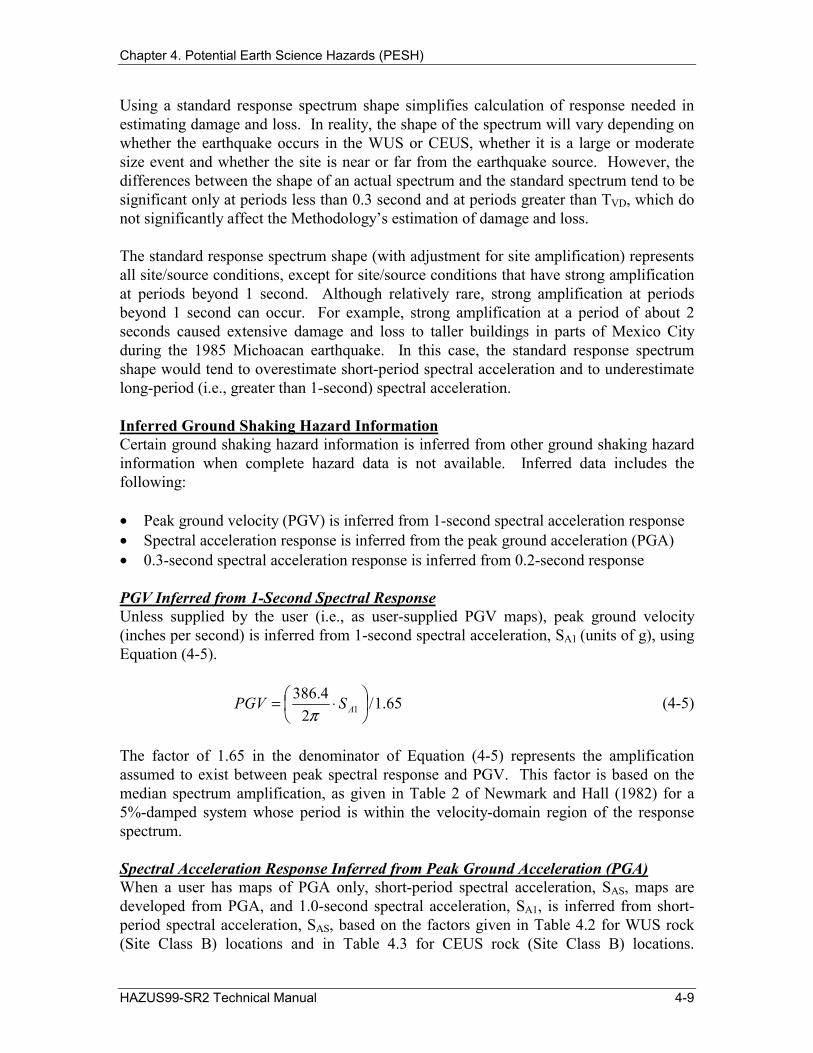
Inferred Ground Shaking Hazard Information Certain ground shaking hazard information is inferred from other ground shaking hazard information when complete hazard data is not available. Inferred data includes the following:
• Peak ground velocity (PGV) is inferred from 1-second spectral acceleration response • Spectral acceleration response is inferred from the peak ground acceleration (PGA) • 0.3-second spectral acceleration response is inferred from 0.2-second response
PGV Inferred from 1-Second Spectral Response Unless supplied by the user (i.e., as user-supplied PGV maps), peak ground velocity (inches per second) is inferred from 1-second spectral acceleration, SA1 (units of g), using Equation (4-5).
386.4 PGV =
2π⋅ S A1 /1.65 (4-5)
The factor of 1.65 in the denominator of Equation (4-5) represents the amplification assumed to exist between peak spectral response and PGV. This factor is based on the median spectrum amplification, as given in Table 2 of Newmark and Hall (1982) for a 5%-damped system whose period is within the velocity-domain region of the response spectrum.
Spectral Acceleration Response Inferred from Peak Ground Acceleration (PGA)When a user has maps of PGA only, short-period spectral acceleration, SAS, maps are developed from PGA, and 1.0-second spectral acceleration, SA1, is inferred from short-period spectral acceleration, SAS, based on the factors given in Table 4.2 for WUS rock (Site Class B) locations and in Table 4.3 for CEUS rock (Site Class B) locations.
HAZUS99-SR2 Technical Manual 4-9

≤≤≤ ≥≥≥ ≤≤≤ ≥≥≥
≤≤≤ ≥≥≥ ≤≤≤ ≥≥≥
Chapter 4. Potential Earth Science Hazards (PESH)
Table 4.2 Spectral Acceleration Response Factors - WUS Rock (Site Class B) Closest Distance to
Fault Rupture SAS/PGA given Magnitude, M: SAS/SA1 given Magnitude, M:
≤ 5 6 7 ≥ 8 ≤ 5 6 7 ≥ 8
≤ 10 km 1.4 1.8 2.1 2.1 5.3 3.7 3.1 1.8
20 km 1.5 2.0 2.1 2.0 5.0 3.5 2.5 1.7 40 km 1.6 2.1 2.2 2.0 4.6 3.3 2.3 1.6
≥ 80 km 1.3 1.8 2.1 2.0 4.1 3.1 2.1 1.5
Table 4.3 Spectral Acceleration Response Factors - CEUS Rock (Site Class B)
Hypocentral Distance
SAS/PGA given Magnitude, M: SAS/SA1 given Magnitude, M:
≤ 5 6 7 ≥ 8 ≤ 5 6 7 ≥ 8
≤ 10 km 0.9 1.2 1.5 2.1 8.7 4.2 3.1 2.3
20 km 1.0 1.3 1.4 1.6 8.1 4.0 3.0 2.7 40 km 1.2 1.4 1.6 1.6 7.3 3.7 2.8 2.6
≥ 80 km 1.5 1.7 1.8 1.9 6.5 3.3 2.5 2.4
The factors given in Tables 4.2 and 4.3 are based on the default combinations of attenuation WUS and CEUS functions, described in the next section. These factors distinguish between small-magnitude and large-magnitude events and between sites that are located at different distances from the source (i.e., closest distance to fault rupture for the WUS and distance to the hypocenter for the CEUS). The ratios of SAS/SA1 and SAS/PGA define the standard shape of the response spectrum for each of the magnitude/distance combinations of Tables 4.2 and 4.3.
Tables 4.2 and 4.3 require magnitude and distance information to determine spectrum amplification factors. This information would likely be available for maps of observed earthquake PGA, or scenario earthquake PGA, but is not available for probabilistic maps of PGA, since these maps are aggregated estimates of seismic hazard due to different event magnitudes and sources.
0.3-Second Spectral Acceleration Response Inferred from 0.2-Second Response Some of the probabilistic maps developed by the USGS for Project 97, estimate short-period spectral response for a period of 0.2 second. Spectral response at a period of 0.3 second is calculated by dividing 0.2-second response by a factor of 1.1 for WUS locations and by dividing 0.2-second response by a factor of 1.4 for CEUS locations.
The factors describing the ratio of 0.2-second and 0.3-second response are based on the default combinations of WUS and CEUS attenuation functions, described in the next section, and the assumption that large-magnitude events tend to dominate seismic hazard at most WUS locations and that small-magnitude events tend to dominate seismic hazard at most CEUS locations.
4-10 HAZUS99-SR2 Technical Manual

Chapter 4. Potential Earth Science Hazards (PESH)
4.1.2.3 Attenuation of Ground Shaking
Ground shaking is attenuated with distance from the source using relationships provided with the Methodology. These relationships define ground shaking for rock (Site Class B) conditions based on earthquake magnitude and other parameters. These relationships are used to estimate PGA and spectral demand at 0.3 and 1.0 seconds, and with the standard response spectrum shape (described in Section 4.1.2.2) fully define 5%-damped demand spectra at a given location.
The Methodology provides five WUS and three CEUS attenuation functions. The WUS relationships should be used for study regions located in, or west of, the Rocky Mountains, Hawaii and Alaska. The CEUS attenuation relationships should be used for the balance of the continental United States and Puerto Rico. Table 3C.1 defines the distribution of states for the WUS and CEUS.
Western United States Attenuation Relationships
The WUS attenuation relationships provided with the Methodology are based on:
• Boore, Joyner & Fumal (1993, 1994a, 1994b) - shallow crustal earthquakes • Sadigh, Chang, Abrahamson, Chiou, and Power (1993) - shallow crustal earthquakes • Campbell and Bozorgnia (1994) - shallow crustal earthquakes (PGA only) • Munson and Thurber (1997) - Hawaiian earthquakes (PGA only) • Youngs, Chiou, Silva and Humphrey (1997) - deep and subduction zone earthquakes
Boore, Joyner and Fumal (1993, 1994a, 1994b)
The Boore, Joyner and Fumal (1993, 1994a, 1994b) attenuation relationships predict PGA and spectral acceleration for different site conditions. In the Methodology, the Boore, Joyner and Fumal (BJF 1994) relationship, given in Equation (4-6), predicts the mean value of ground shaking for a site with a shear wave velocity of VS = 760 m/sec. A shear wave velocity of 760 m/sec is the minimum value of shear wave velocity that defines Site Class B conditions (see Table 4.9), and is the same velocity used by the USGS (Project 97) to develop hazard maps for rock sites (Site Class B).
log10 (SD ) = BSA + aSS
( h r + 2 2
⋅ GSS + aRS ⋅ GRS + b(M − 6) + c(M − 6)2 + d ( h r + 2 2 ) + e[ log 10 ) ] + f (2.881 − log 10VB ) (4-6)
where: SD is mean of the seismic demand (PGA or spectral acceleration (SA) in units of g)
M is the moment magnitude of the earthquake r is the horizontal distance, in km, from the site to the closest point on
the surface projection of fault rupture (see Figure 4.3) BSA is a factor converting spectral velocity (cm/sec) to spectral acc. (g)
HAZUS99-SR2 Technical Manual 4-11
Chapter 4. Potential Earth Science Hazards (PESH)
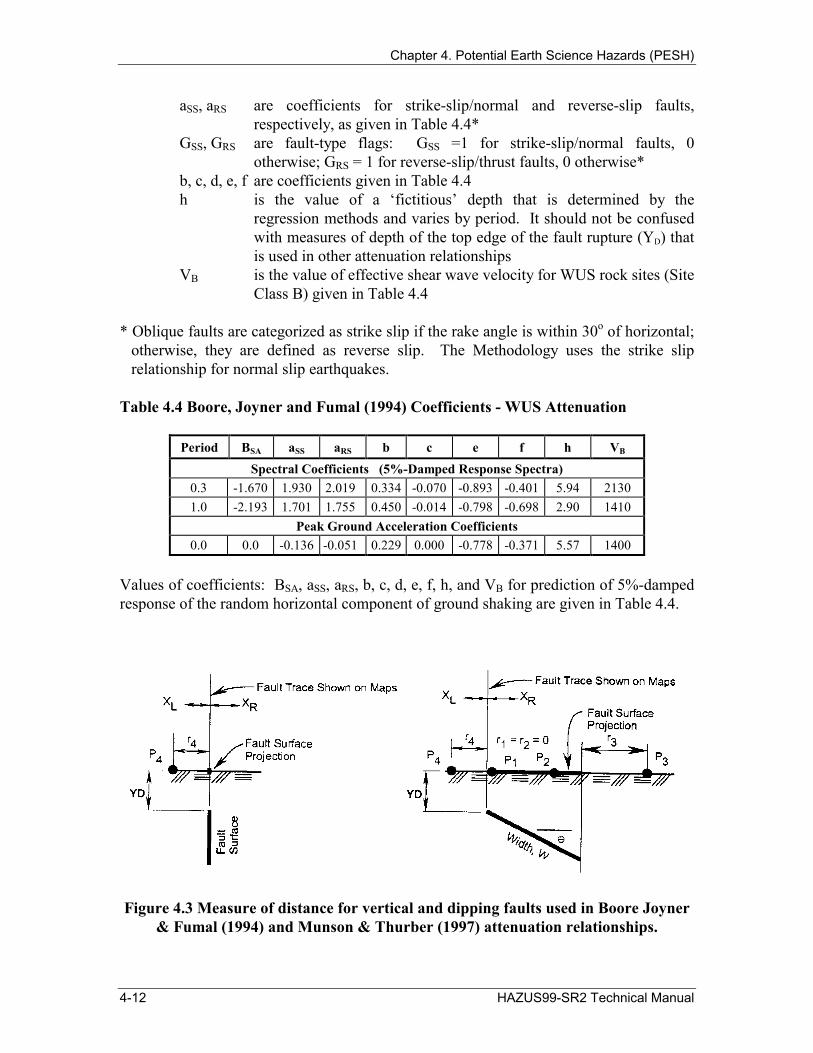
aSS, aRS are coefficients for strike-slip/normal and reverse-slip faults, respectively, as given in Table 4.4*
GSS, GRS are fault-type flags: GSS =1 for strike-slip/normal faults, 0 otherwise; GRS = 1 for reverse-slip/thrust faults, 0 otherwise*
b, c, d, e, f are coefficients given in Table 4.4 h is the value of a ‘fictitious’ depth that is determined by the
regression methods and varies by period. It should not be confused with measures of depth of the top edge of the fault rupture (YD) that is used in other attenuation relationships
VB is the value of effective shear wave velocity for WUS rock sites (Site Class B) given in Table 4.4
* Oblique faults are categorized as strike slip if the rake angle is within 30o of horizontal; otherwise, they are defined as reverse slip. The Methodology uses the strike slip relationship for normal slip earthquakes.
Table 4.4 Boore, Joyner and Fumal (1994) Coefficients - WUS Attenuation
Period BSA aSS aRS b c e f h VB
Spectral Coefficients (5%-Damped Response Spectra) 0.3 -1.670 1.930 2.019 0.334 -0.070 -0.893 -0.401 5.94 2130 1.0 -2.193 1.701 1.755 0.450 -0.014 -0.798 -0.698 2.90 1410
Peak Ground Acceleration Coefficients 0.0 0.0 -0.136 -0.051 0.229 0.000 -0.778 -0.371 5.57 1400
Values of coefficients: BSA, aSS, aRS, b, c, d, e, f, h, and VB for prediction of 5%-damped response of the random horizontal component of ground shaking are given in Table 4.4.
Figure 4.3 Measure of distance for vertical and dipping faults used in Boore Joyner & Fumal (1994) and Munson & Thurber (1997) attenuation relationships.
4-12 HAZUS99-SR2 Technical Manual

Chapter 4. Potential Earth Science Hazards (PESH)
BJF 1994 limits the magnitude range of Equation (4-6) to 5.5 ≤ M ≤ 7.7. BJF 1994 also limits the applicability of Equation (4-6) to source-to-site distances of less than 100 kilometers. In the Methodology, seismic demand for distances greater than 100 kilometers is based on direct substitution of distance into the attenuation relationship (Equations 4-6). The Methodology does not use Equation (4-6) for M > 7.7.
Munson & Thurber (1997)
The Munson and Thurber (1997) attenuation relationship predicts PGA for earthquakes for the Island of Hawaii. In the Methodology, the relationship given in Equation (4-10) is used to predict the mean value of PGA for Site Class B.
log10 (SD ) = −1.804
( r 2 2 29 .11+
+ 0.387(M − 6)− 0.00256 ( r 2 2 29 .11+ ) (4-7)
− log 10 )where: SD is mean of the PGA in units of g
M is the moment magnitude of the earthquake r is the horizontal distance, in km, from the site to the closest point on
the surface projection of fault rupture (see Figure 4.3)
For the Methodology to remain consistent with the USGS approach (Klein et al., 1998), the attenuation relationship for magnitudes greater than 7.0 is modified. From M = 7.0-7.7, the magnitude term becomes 0.316*(7.0) + 0.216*(M-7.0). For M > 7.7, a magnitude term is set to a constant value equal to 0.316*(7.0) + 0.216*(7.7-7.0).
Sadigh, Chang, Abrahamson, Chiou, and Power (1993)
The Sadigh, Chang, Abrahamson, Chiou and Power attenuation relationship (Sadigh 1993) predicts peak ground acceleration and 5%-damped spectral acceleration for rock sites (Site Class B). The relationship is given in Equation (4-8) for events of magnitude M < 6.5 and in Equation (4-9) for events of magnitude M ≥ 6.5.
M < 6.5: ln(SD) = aSS ⋅ GSS + aRS ⋅ GRS + 1.0M + b(8.5 − M )2.5
+ c ln[R + exp(1.29649 + 0.25 ⋅ M )]+ f ⋅ ln(R + 2) (4-8)
HAZUS99-SR2 Technical Manual 4-13

≥≥≥
Chapter 4. Potential Earth Science Hazards (PESH)
M > 6.5: ln(SD) = aSS ⋅ GSS + aRS ⋅ GRS + 1.1M + b(8.5 − M )2.5
(4-9) + c ln[R + exp( −0.48451 + 0.524M )]+ f ⋅ ln(R + 2)
where: SD is the mean value of the seismic demand, PGA or spectral acceleration (SA) in g
M is the moment magnitude of the earthquake R is the distance, in km, to the closest point on the fault rupture surface
(see Figure 4.4) aSS, aRS are coefficients for strike-slip/normal and reverse-slip/thrust faults,
respectively, as given in Table 4.5* GSS, GRS are fault-type flags: GSS =1 for strike-slip/normal faults, 0
otherwise; GRS = 1 for reverse/thrust faults slip, 0 otherwise* b, c, f are coefficients given in Table 4.5
* Oblique faults are categorized as strike slip if the rake angle is within 30o of horizontal; otherwise, they are defined as reverse slip. The Methodology uses the strike slip relationship for normal slip earthquakes.
Table 4.5 Sadigh et al. (1993) Coefficients - WUS Attenuation
Period aSS aRS b c Earthquake Magnitude, M < 6.5
PGA -0.624 -0.442 0.0 -2.100 0.3 -0.057 0.125 -0.017 -2.028 1.0 -1.705 -1.523 -0.055 -1.800
Earthquake Magnitude, M ≥ 6.5 PGA -1.274 -1.092 0.0 -2.100 0.3 -0.707 -0.525 -0.017 -2.028 1.0 -2.355 -2.173 -0.055 -1.800
Sadigh 1993 limits the applicability of Equations 4-7 and 4-8 to earthquake magnitudes M ≤ 8.0. In the Methodology, seismic demand for magnitudes M > 8.0 is based on the Equations 4-7 and 4-8 predictions for M = 8.0.
4-14 HAZUS99-SR2 Technical Manual

Chapter 4. Potential Earth Science Hazards (PESH)
Figure 4.4 Measure of distance for vertical and dipping faults used in Sadigh et al. (1993) attenuation relationships.
Campbell and Bozorgnia (1994)
The Campbell and Bozorgnia (1994) attenuation relationship predicts mean values of PGA for source-to-site distances less than 60 kilometers. The Campbell and Bozorgnia 1994 relationship is given in Equation (4-10) for soft rock site conditions. Soft rock conditions are used by the Methodology for prediction of PGA at rock sites (Soil Class B) in the WUS.
ln(SD) = -3.512 + 0.904Μ − 1.328 ln [ 2 ).6470.149exp(02 R + M ] (4-10) R R+ [1.125 − 0.112ln( )− 0.0957M]⋅ GRS + [0.440 − 0.171ln( )]
where: SD is mean value of the peak ground acceleration (g) M is the moment magnitude of the earthquake R is the closest distance, in km, to zone of seismogenic rupture on the
fault (see Figure 4.5) GRS is a fault type flag: GRS = 1 for reverse-slip faults, 0 otherwise*
* Oblique faults are categorized as strike slip if the rake angle is within 30o of horizontal; else they are defined as reverse slip. The Methodology uses the strike slip relationship for normal slip earthquakes.
The distance R (see Figure 4.5) is measured as the closest distance from the site to the zone of the seismogenic rupture. This definition assumes that fault rupture in the softer sediments of the upper 4 km of the fault is primarily non-seismogenic. The minimum depth is represented as YR in Figure 4.5. In the Methodology, YR is assumed to be a constant of 5 km. As shown in the figure, if YD is less than YR, distances are measured
HAZUS99-SR2 Technical Manual 4-15
Chapter 4. Potential Earth Science Hazards (PESH)
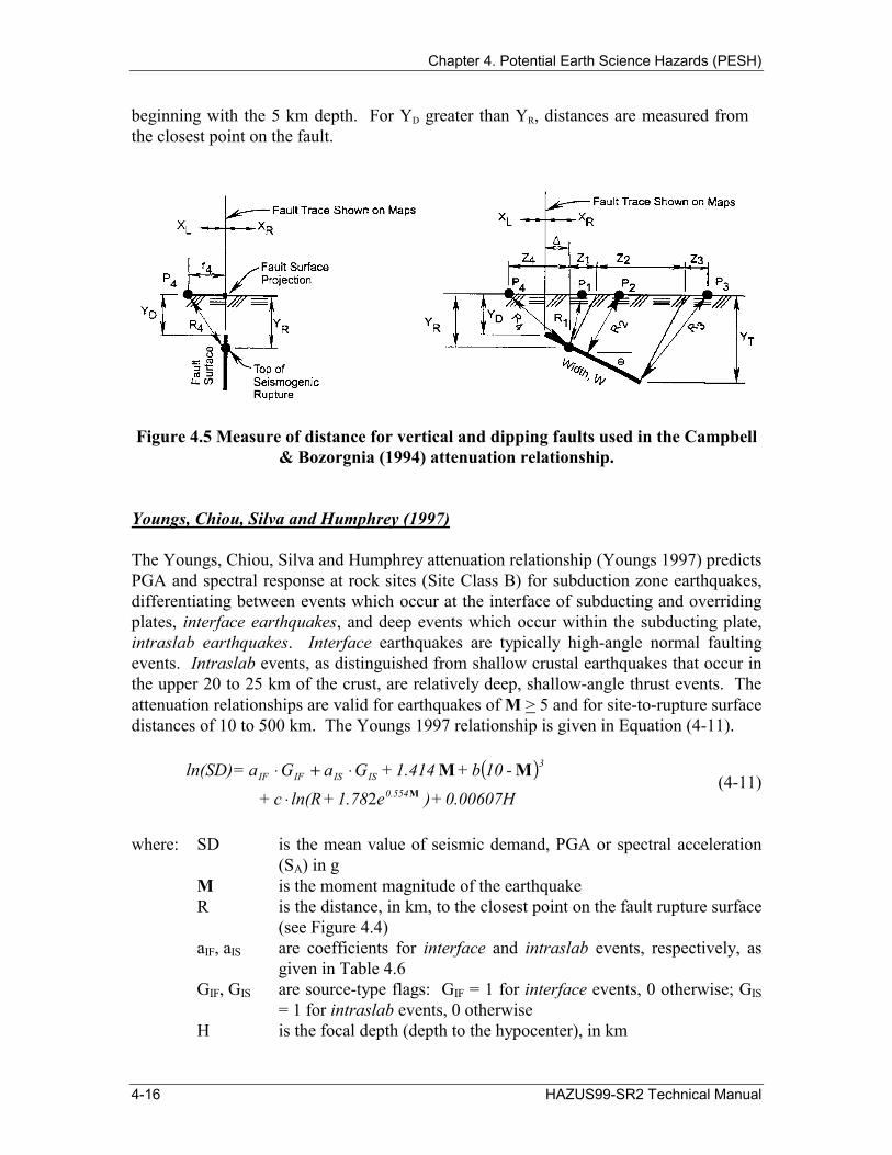
beginning with the 5 km depth. For YD greater than YR, distances are measured from the closest point on the fault.
Figure 4.5 Measure of distance for vertical and dipping faults used in the Campbell & Bozorgnia (1994) attenuation relationship.
Youngs, Chiou, Silva and Humphrey (1997)
The Youngs, Chiou, Silva and Humphrey attenuation relationship (Youngs 1997) predicts PGA and spectral response at rock sites (Site Class B) for subduction zone earthquakes, differentiating between events which occur at the interface of subducting and overriding plates, interface earthquakes, and deep events which occur within the subducting plate, intraslab earthquakes. Interface earthquakes are typically high-angle normal faulting events. Intraslab events, as distinguished from shallow crustal earthquakes that occur in the upper 20 to 25 km of the crust, are relatively deep, shallow-angle thrust events. The attenuation relationships are valid for earthquakes of M > 5 and for site-to-rupture surface distances of 10 to 500 km. The Youngs 1997 relationship is given in Equation (4-11).
ln(SD)= aIF ⋅ GIF + aIS ⋅ GIS +1.414 M +b(10 - M)3
(4-11)+ c ⋅ ln(R +1.782e0.554M )+0.00607H
where: SD is the mean value of seismic demand, PGA or spectral acceleration (SA) in g
M is the moment magnitude of the earthquake R is the distance, in km, to the closest point on the fault rupture surface
(see Figure 4.4) aIF, aIS are coefficients for interface and intraslab events, respectively, as
given in Table 4.6 GIF, GIS are source-type flags: GIF = 1 for interface events, 0 otherwise; GIS
= 1 for intraslab events, 0 otherwise H is the focal depth (depth to the hypocenter), in km
4-16 HAZUS99-SR2 Technical Manual
Chapter 4. Potential Earth Science Hazards (PESH)
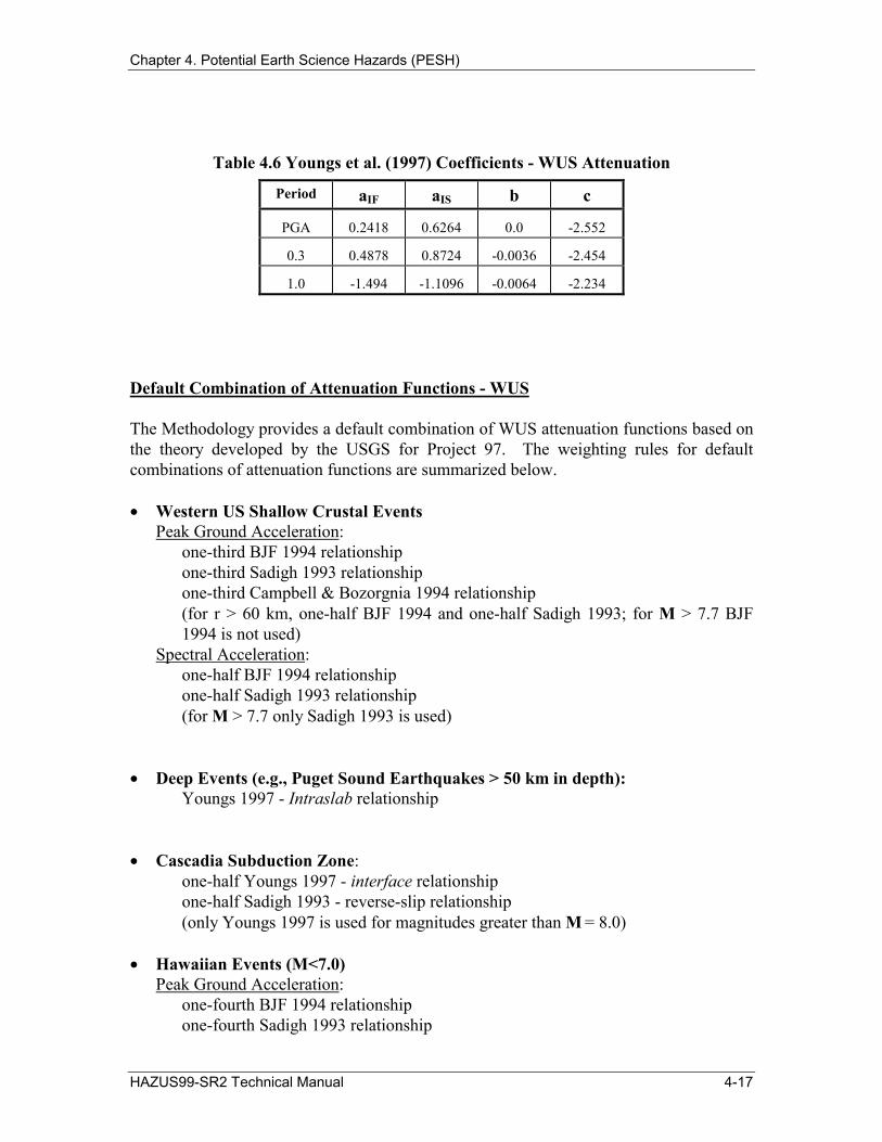
Table 4.6 Youngs et al. (1997) Coefficients - WUS Attenuation
Period aIF aIS b c
PGA 0.2418 0.6264 0.0 -2.552
0.3 0.4878 0.8724 -0.0036 -2.454
1.0 -1.494 -1.1096 -0.0064 -2.234
Default Combination of Attenuation Functions - WUS
The Methodology provides a default combination of WUS attenuation functions based on the theory developed by the USGS for Project 97. The weighting rules for default combinations of attenuation functions are summarized below.
• Western US Shallow Crustal Events Peak Ground Acceleration:
one-third BJF 1994 relationship one-third Sadigh 1993 relationship one-third Campbell & Bozorgnia 1994 relationship (for r > 60 km, one-half BJF 1994 and one-half Sadigh 1993; for M > 7.7 BJF 1994 is not used)
Spectral Acceleration: one-half BJF 1994 relationship one-half Sadigh 1993 relationship (for M > 7.7 only Sadigh 1993 is used)
• Deep Events (e.g., Puget Sound Earthquakes > 50 km in depth): Youngs 1997 - Intraslab relationship
• Cascadia Subduction Zone: one-half Youngs 1997 - interface relationship one-half Sadigh 1993 - reverse-slip relationship (only Youngs 1997 is used for magnitudes greater than M = 8.0)
• Hawaiian Events (M<7.0) Peak Ground Acceleration:
one-fourth BJF 1994 relationship one-fourth Sadigh 1993 relationship
HAZUS99-SR2 Technical Manual 4-17

≥≥≥
Chapter 4. Potential Earth Science Hazards (PESH)
one-fourth Campbell & Bozorgnia 1994 relationship one-fourth Munson & Thurber 1997 relationship
Spectral Acceleration: 0.3 Seconds
one-third BJF 1994 relationship one-third Sadigh 1993 relationship one-third 2.5*( Munson & Thurber 1997 relationship)
1.0 Seconds one-half BJF 1994 relationship one-half Sadigh 1993 relationship
• Hawaiian Events (M≥7.0) Peak Ground Acceleration:
one-half Sadigh 1993 relationship one-half Munson & Thurber 1997 relationship
Spectral Acceleration: 0.3 Seconds
one-half Sadigh 1993 relationship one-half 2.5*( Munson & Thurber 1997 relationship)
1.0 Seconds Sadigh 1993 relationship
Eastern United States Attenuation Relationships
The Central and Eastern U.S. (CEUS) attenuation relationships provided with the Methodology are based on:
• Frankel et al. (Appendix C, Frankel et al., 1996) • Toro, Abrahamson and Schneider (1997) • Lawrence Livermore National Laboratory (Savy, 1998)
For the Eastern United States, the ground shaking attenuation relationships for PGA and spectral acceleration demand are derived from theoretical models, as described in Frankel et al. (1996), Toro, Abrahamson and Schneider (1997) and Savy (1998). The Frankel et al. (1996) attenuation relationship was developed specifically for Project 97. The Toro, Abrahamson and Schneider (1997) relationship was obtained from a paper submitted for publication to Earthquake Spectra. This paper summarizes work of a 1993 study performed by the authors for the Electric Power Research Institute (Toro et al., 1997). Savy (1998) describes the SSHAC expert elicitation methodology used by Lawrence Livermore National Laboratory to develop an attenuation model for hard rock sites in the Eastern United States.
4-18 HAZUS99-SR2 Technical Manual

Chapter 4. Potential Earth Science Hazards (PESH)
Frankel et al. (1996)
The Frankel et al. attenuation relationship (Frankel 1996) predicts PGA and 0.3-second and 1.0-second spectral acceleration response based on simulations of a random vibration stochastic model. Appendix 4A includes tables of mean demand values as published in Frankel et al., 1996, resulting from averaging multiple simulations. Linear interpolation was used to calculate ground motion values for certain magnitudes and distances. These values predict demand for specific event magnitudes ranging from M = 5.0 to M = 8.0 and hypocentral distances ranging from 10 km to 350 km.
The user must specify the hypocentral depth for the Methodology to calculate the hypocentral distance. If not provided by the user, the Methodology assumes a hypocentral depth of 10 km, consistent with the theory of Project 97. Similarly, the Methodology limits the hypocentral distance to a minimum value of 10 km, and limits predicted values of PGA to 1.5g and predicted values of 0.3-second spectral acceleration to 3.75g, consistent with Project 97 theory.
Toro, Abrahamson & Schneider (1997)
The Toro, Abrahamson and Schneider (1997) attenuation relationship predicts PGA, and spectral acceleration for hard rock sites (Site Class A) in the CEUS. For use in the Methodology, the Toro 1997 attenuation relationship includes the following modifications:
• a factor (FAB) is added to increase hard rock (Site Class A) predictions to a level that represents Site Class B (rock) conditions, based on the theory of Project 97
• the hypocentral distance term, RM, is adjusted (i.e., RM is replaced by RM + 0.089e0.6M) to model the saturation effect of extended ruptures on near-fault ground-motion, based on private communication with the authors and previous work by Toro and McGuire (1991)
The Toro 1997 relationship is given in Equation (4-12) with the modified hypocentral distance defined by Equation (4-13).
ln(SD)= a + b( M − 6) + c( M − 6)2 − d ⋅ ln (RM )
− (e − d ) max
ln
RM ,0
− f ⋅ RM + FAB
(4-12)
100
RM = + 2 2 h r + 0.089exp(0.6M) (4-13)
where: SD is the mean value of the seismic demand, PGA or spectral acceleration (SA) in g
HAZUS99-SR2 Technical Manual 4-19
Chapter 4. Potential Earth Science Hazards (PESH)
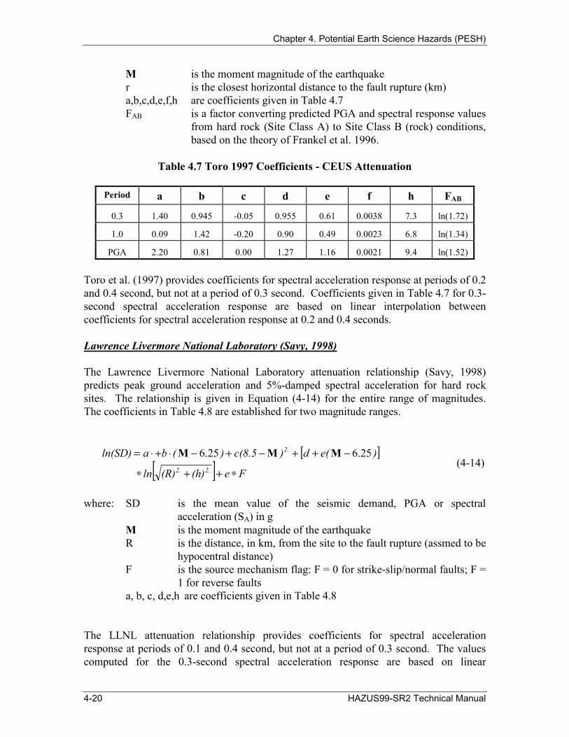
M is the moment magnitude of the earthquaker is the closest horizontal distance to the fault rupture (km)a,b,c,d,e,f,h are coefficients given in Table 4.7 FAB is a factor converting predicted PGA and spectral response values
from hard rock (Site Class A) to Site Class B (rock) conditions, based on the theory of Frankel et al. 1996.
Table 4.7 Toro 1997 Coefficients - CEUS Attenuation
Period a b c d e f h FAB
0.3 1.40 0.945 -0.05 0.955 0.61 0.0038 7.3 ln(1.72)
1.0 0.09 1.42 -0.20 0.90 0.49 0.0023 6.8 ln(1.34)
PGA 2.20 0.81 0.00 1.27 1.16 0.0021 9.4 ln(1.52)
Toro et al. (1997) provides coefficients for spectral acceleration response at periods of 0.2 and 0.4 second, but not at a period of 0.3 second. Coefficients given in Table 4.7 for 0.3-second spectral acceleration response are based on linear interpolation between coefficients for spectral acceleration response at 0.2 and 0.4 seconds.
Lawrence Livermore National Laboratory (Savy, 1998)
The Lawrence Livermore National Laboratory attenuation relationship (Savy, 1998) predicts peak ground acceleration and 5%-damped spectral acceleration for hard rock sites. The relationship is given in Equation (4-14) for the entire range of magnitudes. The coefficients in Table 4.8 are established for two magnitude ranges.
ln(SD) = a ⋅ +b ⋅ ( M − 6.25 ) + c(8.5 − M )2. + [d + e( M − 6.25 )] ∗ ln[ (R)2. + (h)2. ]+ e ∗ F
(4-14)
where: SD is the mean value of the seismic demand, PGA or spectral acceleration (SA) in g
M is the moment magnitude of the earthquake R is the distance, in km, from the site to the fault rupture (assmed to be
hypocentral distance) F is the source mechanism flag: F = 0 for strike-slip/normal faults; F =
1 for reverse faults a, b, c, d,e,h are coefficients given in Table 4.8
The LLNL attenuation relationship provides coefficients for spectral acceleration response at periods of 0.1 and 0.4 second, but not at a period of 0.3 second. The values computed for the 0.3-second spectral acceleration response are based on linear
4-20 HAZUS99-SR2 Technical Manual

≥≥≥
Chapter 4. Potential Earth Science Hazards (PESH)
interpolation between coefficients for spectral acceleration response at 0.1 and 0.4 seconds. Since the current version of HAZUS does not distinguish between source mechanisms for earthquakes in the Central and Eastern United States, the values computed for PGA and spectral acceleration response are the average between the strike slip and normal mechanisms.
Table 4.8 Lawrence Livermore National Laboratory Coefficients – CEUS Attenuation (Savy, 1998)
Period a b c d e e h Earthquake Magnitude, M < 6.25
PGA 3.267 0.294 0.000 -1.446 0.146 0.015 9.2 0.1 3.580 0.294 -0.008 -1.354 0.146 0.021 9.1 0.4 2.349 0.294 -0.072 -1.138 0.146 0.065 7.7 1.0 1.464 0.294 -0.136 -1.061 0.146 -0.012 7.0
Earthquake Magnitude, M ≥ 6.25 PGA 3.267 0.127 0.000 -1.446 0.146 0.015 9.2 0.1 3.580 0.127 -0.008 -1.354 0.146 0.021 9.1 0.4 2.349 0.127 -0.072 -1.138 0.146 0.065 7.7 1.0 1.464 0.127 -0.136 -1.061 0.146 -0.012 7.0
Default Combination of Attenuation Functions - CEUS
The Methodology provides a default combination of CEUS attenuation functions based on the theory developed by the USGS for Project 97. The Lawrence Livermore National Laboratory relationship was not used by the USGS in Project 97. The weighting rules for default combinations of attenuation functions are summarized below.
• Peak Ground Acceleration: one-half Frankel 1996 relationship one-half Toro 1997 relationship
• Spectral Acceleration: one-half Frankel 1996 relationship one-half Toro 1997 relationship
The default combination of CEUS attenuation functions predict significantly stronger ground shaking than the default combination of WUS attenuation functions for the same scenario earthquake (i.e., same moment magnitude and distance to source). For example, Figure 4.6 compares WUS and CEUS rock (Site Class B) response spectra (standard shape) for a magnitude M = 7.0 earthquake at 20 km from the source. As illustrated in
HAZUS99-SR2 Technical Manual 4-21

Chapter 4. Potential Earth Science Hazards (PESH)
Figure 4.6, CEUS spectral demand is about 2.0 times WUS demand in the acceleration domain and between 1.5 to 2.0 times WUS demand in the velocity domain.
1
0.9
0.8
0.7
0.6
0.5
0.4
0.3
0.2
0.1
0
WUS - Site Class B (SS/RS)
CEUS - Site Class B
0.3 sec.
1.0 sec.
WUS PGA = 0.20g
CEUS PGA = 0.61g
0 1 2 3 4 5 6 7 8 9 10 Spectral Displacement (inches)
Figure 4.6 Example Comparison of WUS and CEUS Spectra - Site Class B (M = 7.0 at 20 km - Default Combination of Attenuation).
4.1.2.4 Amplification of Ground Shaking - Local Site Conditions
Amplification of ground shaking to account for local site conditions is based on the site classes and soil amplification factors proposed for the 1997 NEHRP Provisions (which are essentially the same as the 1994 NEHRP Provisions, FEMA 222A, 1995). The NEHRP Provisions define a standardized site geology classification scheme and specify soil amplification factors for most site classes. The classification scheme of the NEHRP Provisions is based, in part, on the average shear wave velocity of the upper 30 meters of the local site geology, as shown in Table 4.9. Users (with geotechnical expertise) are required to relate the soil classification scheme of soil maps to the classification scheme shown in Table 4.9.
Spec
tral
Acc
eler
atio
n (g
's)
4-22 HAZUS99-SR2 Technical Manual
Chapter 4. Potential Earth Science Hazards (PESH)
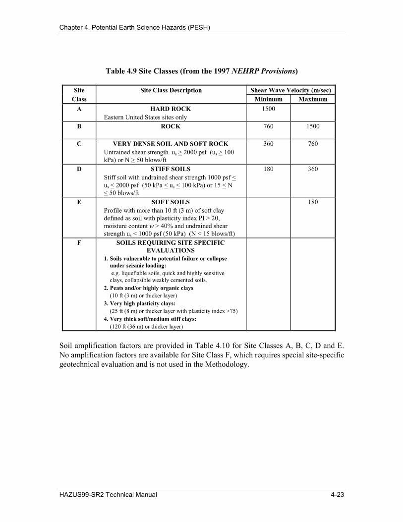
Table 4.9 Site Classes (from the 1997 NEHRP Provisions)
Site Class
Site Class Description Shear Wave Velocity (m/sec) Minimum Maximum
A HARD ROCK Eastern United States sites only
1500
B ROCK 760 1500
C VERY DENSE SOIL AND SOFT ROCK Untrained shear strength us > 2000 psf (us > 100 kPa) or N > 50 blows/ft
360 760
D STIFF SOILS Stiff soil with undrained shear strength 1000 psf < us < 2000 psf (50 kPa < us < 100 kPa) or 15 < N < 50 blows/ft
180 360
E SOFT SOILS Profile with more than 10 ft (3 m) of soft clay defined as soil with plasticity index PI > 20, moisture content w > 40% and undrained shear strength us < 1000 psf (50 kPa) (N < 15 blows/ft)
180
F SOILS REQUIRING SITE SPECIFIC EVALUATIONS
1. Soils vulnerable to potential failure or collapse under seismic loading: e.g. liquefiable soils, quick and highly sensitive
clays, collapsible weakly cemented soils. 2. Peats and/or highly organic clays
(10 ft (3 m) or thicker layer) 3. Very high plasticity clays:
(25 ft (8 m) or thicker layer with plasticity index >75) 4. Very thick soft/medium stiff clays:
(120 ft (36 m) or thicker layer)
Soil amplification factors are provided in Table 4.10 for Site Classes A, B, C, D and E. No amplification factors are available for Site Class F, which requires special site-specific geotechnical evaluation and is not used in the Methodology.
HAZUS99-SR2 Technical Manual 4-23
Chapter 4. Potential Earth Science Hazards (PESH)
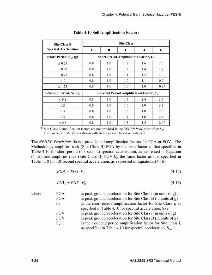
Table 4.10 Soil Amplification Factors
Site Class B Spectral Acceleration
Site Class
A B C D E
Short-Period, SAS (g) Short-Period Amplification Factor, FA
≤ 0.25 0.8 1.0 1.2 1.6 2.5
0.50 0.8 1.0 1.2 1.4 1.7
0.75 0.8 1.0 1.1 1.2 1.2
1.0 0.8 1.0 1.0 1.1 0.9
≥ 1.25 0.8 1.0 1.0 1.0 0.8*
1-Second Period, SA1 (g) 1.0-Second Period Amplification Factor, FV
≤ 0.1 0.8 1.0 1.7 2.4 3.5
0.2 0.8 1.0 1.6 2.0 3.2
0.3 0.8 1.0 1.5 1.8 2.8
0.4 0.8 1.0 1.4 1.6 2.4
≥ 0.5 0.8 1.0 1.3 1.5 2.0*
* Site Class E amplification factors are not provided in the NEHRP Provisions when SAS > 1.0 or SA1 > 0.4. Values shown with an asterisk are based on judgment.
The NEHRP Provisions do not provide soil amplification factors for PGA or PGV. The Methodology amplifies rock (Site Class B) PGA by the same factor as that specified in Table 4.10 for short-period (0.3-second) spectral acceleration, as expressed in Equation (4-15), and amplifies rock (Site Class B) PGV by the same factor as that specified in Table 4.10 for 1.0-second spectral acceleration, as expressed in Equations (4-16).
PGAi = PGA ⋅ FAi (4-15)
PGVi = PGV ⋅ FVi (4-16)
where: PGAi is peak ground acceleration for Site Class i (in units of g) PGA is peak ground acceleration for Site Class B (in units of g) FAi is the short-period amplification factor for Site Class i, as
specified in Table 4.10 for spectral acceleration, SAS PGVi is peak ground acceleration for Site Class i (in units of g) PGV is peak ground acceleration for Site Class B (in units of g) FVi is the 1-second period amplification factor for Site Class i,
as specified in Table 4.10 for spectral acceleration, SA1
4-24 HAZUS99-SR2 Technical Manual
Chapter 4. Potential Earth Science Hazards (PESH)
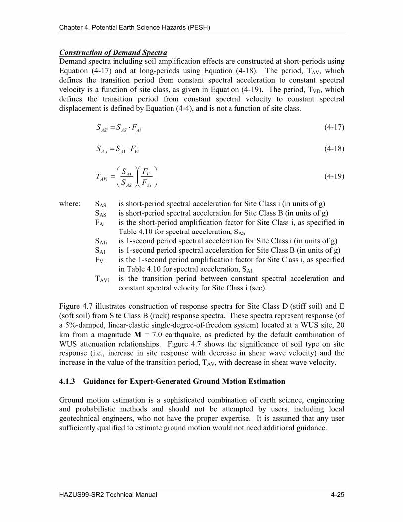
Construction of Demand Spectra Demand spectra including soil amplification effects are constructed at short-periods using Equation (4-17) and at long-periods using Equation (4-18). The period, TAV, which defines the transition period from constant spectral acceleration to constant spectral velocity is a function of site class, as given in Equation (4-19). The period, TVD, which defines the transition period from constant spectral velocity to constant spectral displacement is defined by Equation (4-4), and is not a function of site class.
S ASi = S AS ⋅ FAi (4-17)
S A1i = S A1 ⋅ FVi (4-18)
S A1 FVi TAVi = S AS
FAi
(4-19)
where: SASi is short-period spectral acceleration for Site Class i (in units of g) SAS is short-period spectral acceleration for Site Class B (in units of g) FAi is the short-period amplification factor for Site Class i, as specified in
Table 4.10 for spectral acceleration, SAS SA1i is 1-second period spectral acceleration for Site Class i (in units of g) SA1 is 1-second period spectral acceleration for Site Class B (in units of g) FVi is the 1-second period amplification factor for Site Class i, as specified
in Table 4.10 for spectral acceleration, SA1 TAVi is the transition period between constant spectral acceleration and
constant spectral velocity for Site Class i (sec).
Figure 4.7 illustrates construction of response spectra for Site Class D (stiff soil) and E (soft soil) from Site Class B (rock) response spectra. These spectra represent response (of a 5%-damped, linear-elastic single-degree-of-freedom system) located at a WUS site, 20 km from a magnitude M = 7.0 earthquake, as predicted by the default combination of WUS attenuation relationships. Figure 4.7 shows the significance of soil type on site response (i.e., increase in site response with decrease in shear wave velocity) and the increase in the value of the transition period, TAV, with decrease in shear wave velocity.
4.1.3 Guidance for Expert-Generated Ground Motion Estimation
Ground motion estimation is a sophisticated combination of earth science, engineering and probabilistic methods and should not be attempted by users, including local geotechnical engineers, who not have the proper expertise. It is assumed that any user sufficiently qualified to estimate ground motion would not need additional guidance.
HAZUS99-SR2 Technical Manual 4-25

Chapter 4. Potential Earth Science Hazards (PESH)
1
0.9
0.8
0.7
0.6
0.5
0.4
0.3
0.2
0.1
0
Site Class B (Rock) Site Class D (Stiff Soil) Site Class E (Soft Soil)
0.3 sec.
1.0 sec.
SA1 x FVE
SA1 x FVD
SAS x FAE
SAS x FAD
SAS
SA1
0 1 2 3 4 5 6 7 8 9 10 Spectral Displacement (inches)
Figure 4.7 Example Construction of Site Class B, C and D Spectra - WUS (M = 7.0 at 20 km - Default Combination of Attenuation).
4.2 Ground Failure 4.2.1 Introduction
Three types of ground failure are considered: liquefaction, landsliding and surface fault rupture. Each of these types of ground failure are quantified by permanent ground deformation (PGD). Methods and alternatives for determining PGD due to each mode of ground failure are discussed below.
4.2.1.1 Scope
The scope of this section is to provide methods for evaluating the ground failure hazards of: (a) liquefaction, (b) landsliding, and (c) surface fault rupture. The evaluation of the hazard includes the probability of the hazard occurring and the resulting ground displacement.
4.2.1.2 Input Requirements and Output Information
Input Liquefaction • A geologic map based on the age, depositional environment, and possibly the material
characteristics of the geologic units will be used with Table 4.11 to create a liquefaction susceptibility map
• Groundwater depth map is supplied with a default depth of 5 feet.
Spec
tral
Acc
eler
atio
n (g
's)
4-26 HAZUS99-SR2 Technical Manual

Chapter 4. Potential Earth Science Hazards (PESH)
• Earthquake Moment Magnitude (M) Landsliding • A geologic map, a topographic map, and a map with ground water conditions will be
used with Table 4.16 to produce a landslide susceptibility map • Earthquake Moment Magnitude (M) Surface Fault Rupture • Location of the surface trace of a segment of an active fault that is postulated
to rupture during the scenario earthquake
OutputLiquefaction, and Landsliding
• Aerial depiction map depicting estimated permanent ground deformations. Surface Fault Rupture
• No maps are generated, only site-specific demands are determined.
4.2.2 Description of Methods
4.2.2.1 Liquefaction
4.2.2.1.1 Background
Liquefaction is a soil behavior phenomenon in which a saturated soil looses a substantial amount of strength due to high excess pore-water pressure generated by and accumulated during strong earthquake ground shaking.
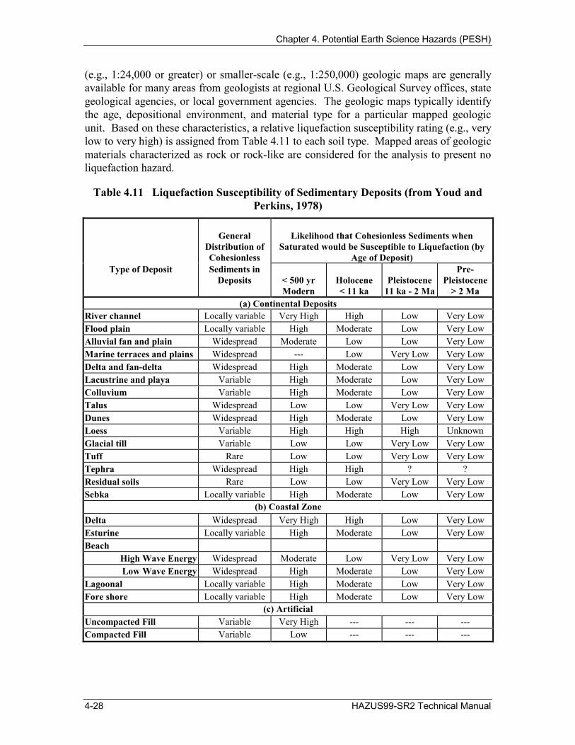
Youd and Perkins (1978) have addressed the liquefaction susceptibility of various types of soil deposits by assigning a qualitative susceptibility rating based upon general depositional environment and geologic age of the deposit. The relative susceptibility ratings of Youd and Perkins (1978) shown in Table 4.11 indicate that recently deposited relatively unconsolidated soils such as Holocene-age river channel, flood plain, and delta deposits and uncompacted artificial fills located below the groundwater table have high to very high liquefaction susceptibility. Sands and silty sands are particularly susceptible to liquefaction. Silts and gravels also are susceptible to liquefaction, and some sensitive clays have exhibited liquefaction-type strength losses (Updike, et. al., 1988).
Permanent ground displacements due to lateral spreads or flow slides and differential settlement are commonly considered significant potential hazards associated with liquefaction.
4.2.2.1.2 Liquefaction Susceptibility
The initial step of the liquefaction hazard evaluation is to characterize the relative liquefaction susceptibility of the soil/geologic conditions of a region or subregion. Susceptibility is characterized utilizing geologic map information and the classification system presented by Youd and Perkins (1978) as summarized in Table 4.11. Large-scale
HAZUS99-SR2 Technical Manual 4-27
--
--- ---
-
--- --- --- ---
Chapter 4. Potential Earth Science Hazards (PESH)
(e.g., 1:24,000 or greater) or smaller-scale (e.g., 1:250,000) geologic maps are generally available for many areas from geologists at regional U.S. Geological Survey offices, state geological agencies, or local government agencies. The geologic maps typically identify the age, depositional environment, and material type for a particular mapped geologic unit. Based on these characteristics, a relative liquefaction susceptibility rating (e.g., very low to very high) is assigned from Table 4.11 to each soil type. Mapped areas of geologic materials characterized as rock or rock-like are considered for the analysis to present no liquefaction hazard.
Table 4.11 Liquefaction Susceptibility of Sedimentary Deposits (from Youd and Perkins, 1978)
Type of Deposit
General Distribution of Cohesionless Sediments in
Deposits
Likelihood that Cohesionless Sediments when Saturated would be Susceptible to Liquefaction (by
Age of Deposit)
< 500 yr Modern
Holocene < 11 ka
Pleistocene 11 ka - 2 Ma
Pre-Pleistocene
> 2 Ma (a) Continental Deposits
River channel Locally variable Very High High Low Very Low Flood plain Locally variable High Moderate Low Very Low Alluvial fan and plain Widespread Moderate Low Low Very Low Marine terraces and plains Widespread Low Very Low Very Low Delta and fan-delta Widespread High Moderate Low Very Low Lacustrine and playa Variable High Moderate Low Very Low Colluvium Variable High Moderate Low Very Low Talus Widespread Low Low Very Low Very Low Dunes Widespread High Moderate Low Very Low Loess Variable High High High Unknown Glacial till Variable Low Low Very Low Very Low Tuff Rare Low Low Very Low Very Low Tephra Widespread High High ? ? Residual soils Rare Low Low Very Low Very Low Sebka Locally variable High Moderate Low Very Low
(b) Coastal Zone Delta Widespread Very High High Low Very Low Esturine Locally variable High Moderate Low Very Low Beach
High Wave Energy Widespread Moderate Low Very Low Very Low Low Wave Energy Widespread High Moderate Low Very Low
Lagoonal Locally variable High Moderate Low Very Low Fore shore Locally variable High Moderate Low Very Low
(c) Artificial Uncompacted Fill Variable Very High Compacted Fill Variable Low
4-28 HAZUS99-SR2 Technical Manual

Chapter 4. Potential Earth Science Hazards (PESH)
Liquefaction susceptibility maps produced for certain regions [e.g., greater San Francisco region (ABAG, 1980); San Diego (Power, et. al., 1982); Los Angeles (Tinsley, et. al., 1985); San Jose (Power, et. al., 1991); Seattle (Grant, et. al., 1991); among others] are also available and may alternatively be utilized in the hazard analysis.
4.2.2.1.3 Probability of Liquefaction
The likelihood of experiencing liquefaction at a specific location is primarily influenced by the susceptibility of the soil, the amplitude and duration of ground shaking and the depth of groundwater. The relative susceptibility of soils within a particular geologic unit is assigned as previously discussed. It is recognized that in reality, natural geologic deposits as well as man-placed fills encompass a range of liquefaction susceptibilities due to variations of soil type (i.e., grain size distribution), relative density, etc. Therefore, portions of a geologic map unit may not be susceptible to liquefaction, and this should be considered in assessing the probability of liquefaction at any given location within the unit. In general, we expect non-susceptible portions to be smaller for higher susceptibilities. This "reality" is incorporated by a probability factor that quantifies the proportion of a geologic map unit deemed susceptible to liquefaction (i.e., the likelihood of susceptible conditions existing at any given location within the unit). For the various susceptibility categories, suggested default values are provided in Table 4.12.
Table 4.12 Proportion of Map Unit Susceptible to Liquefaction
Mapped Relative Susceptibility Proportion of Map Unit Very High 0.25
High 0.20 Moderate 0.10
Low 0.05 Very Low 0.02
None 0.00
These values reflect judgments developed based on preliminary examination of soil properties data sets compiled for geologic map units characterized for various regional liquefaction studies (e.g., Power, et. al., 1992; Geomatrix, 1993).
As previously stated, the likelihood of liquefaction is significantly influenced by ground shaking amplitude (i.e., peak horizontal acceleration, PGA), ground shaking duration as reflected by earthquake magnitude, M, and groundwater depth. Thus, the probability of liquefaction for a given susceptibility category can be determined by the following relationship:
P LiquefactionSC = P LiquefactionSC PGA = a
⋅ Pml (4-20)KM ⋅ Kw
where
HAZUS99-SR2 Technical Manual 4-29

Chapter 4. Potential Earth Science Hazards (PESH)
P LiquefactionSC PGA = a is the conditional liquefaction probability for a given susceptibility category at a specified level of peak ground acceleration (See Figure 4.8)
KM is the moment magnitude (M) correction factor (Equation 4-21) Kw is the ground water correction factor (Equation 4-22) Pml proportion of map unit susceptible to liquefaction (Table 4.12)
Relationships between liquefaction probability and peak horizontal ground acceleration (PGA) are defined for the given susceptibility categories in Table 4.13 and also represented graphically in Figure 4.8. These relationships have been defined based on the state-of-practice empirical procedures, as well as the statistical modeling of the empirical liquefaction catalog presented by Liao, et. al. (1988) for representative penetration resistance characteristics of soils within each susceptibility category (See Section 4.2.3.2.3) as gleaned from regional liquefaction studies cited previously. Note that the relationships given in Figure 4.8 are simplified representations of the relationships that would be obtained using Liao, et al. (1988) or empirical procedures.
Figure 4.8 Conditional Liquefaction Probability Relationships for Liquefaction Susceptibility Categories (after Liao, et. al., 1988).
Peak Horizontal Ground Acceleration, PGA (g)
P[L|
PGA
=a]
0
0.25
0.5
0.75
1
0 0.1 0.2 0.3 0.4 0.5 0.6
Very High
High
Moderate
Low
Very Low
4-30 HAZUS99-SR2 Technical Manual

Chapter 4. Potential Earth Science Hazards (PESH)
Table 4.13 Conditional Probability Relationship for Liquefaction Susceptibility Categories
Susceptibility Category [ ]P Liquefaction PGA a=
Very High 0 ≤ 9.09 a - 0.82 ≤ 1.0 High 0 ≤ 7.67a - 0.92 ≤ 1.0
Moderate 0 ≤ 6.67a -1.0 ≤ 1.0 Low 0 ≤ 5.57a -1.18 ≤ 1.0
Very Low 0 ≤ 4.16a - 1.08 ≤ 1.0 None 0.0
The conditional liquefaction probability relationships presented in Figure 4.8 were developed for a M =7.5 earthquake and an assumed groundwater depth of five feet Correction factors to account for other moment magnitudes (M) and groundwater depths are given by Equations 4-21 and 4-22 respectively. These modification factors are well recognized and have been explicitly incorporated in state-of-practice empirical procedures for evaluating the liquefaction potential (Seed and Idriss, 1982; Seed, et. al., 1985; National Research Council, 1985). These relationships are also presented graphically in Figures 4.9 and 4.10. The magnitude and groundwater depth corrections are made automatically in the methodology. The modification factors can be computed using the following relationships:
Km = 0.0027M3 − 0.0267M 2 − 0.2055M + 2.9188 (4-21)
Kw = 0.022d w + 0 93 (4-22).
where: Km is the correction factor for moment magnitudes other than M=7.5; Kw is the correction factor for groundwater depths other than five feet; M represents the magnitude of the seismic event, and; dw represents the depth to the groundwater in feet.
HAZUS99-SR2 Technical Manual 4-31

Chapter 4. Potential Earth Science Hazards (PESH)
Earthquake Magnitude, M
Km
0.0
1.0
2.0
4 7 6 5 8
Figure 4.9 Moment Magnitude (M) Correction Factor for Liquefaction Probability Relationships (after Seed and Idriss, 1982).
2.0
1.0
0.0 0 10 20 30 40
Depth to Groundwater, dw (feet)
Kw
Figure 4.10 Ground Water Depth Correction Factor for Liquefaction Probability Relationships.
4-32 HAZUS99-SR2 Technical Manual

Chapter 4. Potential Earth Science Hazards (PESH)
4.2.2.1.4 Permanent Ground Displacements
Lateral Spreading The expected permanent ground displacements due to lateral spreading can be determined using the following relationship:
E[PGDSC ] = K∆ ⋅ E[ PGD (PGA / PLSC ) = a ] (4-23) where
E PGD (PGA / PLSC ) = a ] is the expected permanent ground displacement for a[ given susceptibility category under a specified level of normalized ground shaking (PGA/PGA(t)) (Figure 4.11)
PGA(t) is the threshold ground acceleration necessary to induce liquefaction (Table 4.14)
K∆ is the displacement correction factor given by Equation 4-24
This relationship for lateral spreading was developed by combining the Liquefaction Severity Index (LSI) relationship presented by Youd and Perkins (1987) with the ground motion attenuation relationship developed by Sadigh, et. al. (1986) as presented in Joyner and Boore (1988). The ground shaking level in Figure 4.11 has been normalized by the threshold peak ground acceleration PGA(t) corresponding to zero probability of liquefaction for each susceptibility category as shown on Figure 4.8. The PGA(t) values for different susceptibility categories are summarized in Table 4.14.
The displacement term, E PGD ( PGA / PLSC ) = a ] , in Equation 4-23 is based on M =[ 7.5 earthquakes. Displacements for other magnitudes are determined by modifying this displacement term by the displacement correction factor given by Equation 4-24. This equation is based on work done by Seed & Idriss (1982). The displacement correction factor, K∆, is shown graphically in Figure 4.12.
K ∆ = 0.0086M3 − 0.0914M2 + 0.4698M − 0.9835 (4-24)
where M is moment magnitude.
HAZUS99-SR2 Technical Manual 4-33

Chapter 4. Potential Earth Science Hazards (PESH)
0
20
40
60
80
100
0 3
PGA/PGA(t)
Dis
plac
emen
t (in
ches
) 12x - 12 GA/PGA(t)< 2 18x - 24 GA/PGA(t)< 3 70x - 180 GA/PGA(t)< 4
2 1 5 4
1< Pfor 2< Pfor 3< Pfor
Figure 4.11 Lateral Spreading Displacement Relationship (after Youd and Perkins, 1978; Sadigh, et. al., 1986).
Table 4.14 Threshold Ground Acceleration (PGA(t)) Corresponding to Zero Probability of Liquefaction
Susceptibility Category PGA(t) Very High 0.09g
High 0.12g Moderate 0.15g
Low 0.21g Very Low 0.26g
None N/A
4-34 HAZUS99-SR2 Technical Manual
∆∆∆,,,
Chapter 4. Potential Earth Science Hazards (PESH)
2
1
0 4 5 6 7 8
Earthquake Magnitude, M
Dis
plac
emen
t Cor
rect
ion
Fact
or
Figure 4.12 Displacement Correction Factor, K∆, for Lateral Spreading Displacement Relationships (after Seed & Idriss, 1982).
Ground Settlement
Ground settlement associated with liquefaction is assumed to be related to the susceptibility category assigned to an area. This assumption is consistent with relationships presented by Tokimatsu and Seed (1987) and Ishihara (1991) that indicate strong correlations between volumetric strain (settlement) and soil relative density (a measure of susceptibility). Additionally, experience has shown that deposits of higher susceptibility tend to have increased thicknesses of potentially liquefiable soils. Based on these considerations, the ground settlement amplitudes are given in Table 4.15 for the portion of a soil deposit estimated to experience liquefaction at a given ground motion level. The uncertainty associated with these settlement values is assumed to have a uniform probability distribution within bounds of one-half to two times the respective value. It is noted that the relationships presented by Tokimatsu and Seed (1987) and Ishihara (1991) demonstrate very little dependence of settlement on ground motion level given the occurrence of liquefaction. The expected settlement at a location, therefore, is the product of the probability of liquefaction (Equation 4-18) for a given ground motion level and the characteristic settlement amplitude appropriate to the susceptibility category (Table 4.15).
HAZUS99-SR2 Technical Manual 4-35
Chapter 4. Potential Earth Science Hazards (PESH)
Table 4.15 Ground Settlement Amplitudes for Liquefaction Susceptibility Categories
Relative Susceptibility Settlement (inches) Very High 12
High 6 Moderate 2
Low 1 Very Low 0
None 0
4.2.2.2 Landslide
4.2.2.2.1 Background
Earthquake-induced landsliding of a hillside slope occurs when the static plus inertia forces within the slide mass cause the factor of safety to temporarily drop below 1.0. The value of the peak ground acceleration within the slide mass required to just cause the factor of safety to drop to 1.0 is denoted by the critical or yield acceleration ac. This value of acceleration is determined based on pseudo-static slope stability analyses and/or empirically based on observations of slope behavior during past earthquakes.
Deformations are calculated using the approach originally developed by Newmark (1965). The sliding mass is assumed to be a rigid block. Downslope deformations occur during the time periods when the induced peak ground acceleration within the slide mass ais exceeds the critical acceleration ac. The accumulation of displacement is illustrated in Figure 4.13. In general, the smaller the ratio (below 1.0) of ac to ais, the greater is the number and duration of times when downslope movement occurs, and thus the greater is the total amount of downslope movement. The amount of downslope movement also depends on the duration or number of cycles of ground shaking. Since duration and number of cycles increase with earthquake magnitude, deformation tends to increase with increasing magnitude for given values of ac and ais.
4.2.2.2.2 Landslide Susceptibility
The landslide hazard evaluation requires the characterization of the landslide susceptibility of the soil/geologic conditions of a region or subregion. Susceptibility is
4-36 HAZUS99-SR2 Technical Manual
Chapter 4. Potential Earth Science Hazards (PESH)
ky1 ky2 ky3
t2t1 t
Acceleration
t
Velocity
t
t1 t3
t1 t3
Displacement
Note: Critical accelerations in figure are ky1, ky2 and ky3. acceleration is usually taken as a single value.
In applications, critical
Figure 4.13 Integration of Accelerograms to Determine Downslope Displacements (Goodman and Seed, 1966).
HAZUS99-SR2 Technical Manual 4-37
Chapter 4. Potential Earth Science Hazards (PESH)
characterized by the geologic group, slope angle and critical acceleration. The acceleration required to initiate slope movement is a complex function of slope geology, steepness, groundwater conditions, type of landsliding and history of previous slope performance. At the present time, a generally accepted relationship or simplified methodology for estimating ac has not been developed.
The relationship proposed by Wilson and Keefer (1985) is utilized in the methodology. This relationship is shown in Figure 4.14. Landslide susceptibility is measured on a scale of I to X, with I being the least susceptible. The site condition is identified using three geologic groups and groundwater level. The description for each geologic group and its associated susceptibility is given in Table 4.16. The groundwater condition is divided into either dry condition (groundwater below level of the sliding) or wet condition (groundwater level at ground surface). The critical acceleration is then estimated for the respective geologic and groundwater conditions and the slope angle. To avoid calculating the occurrence of landsliding for very low or zero slope angles and critical accelerations, lower bounds for slope angles and critical accelerations are established. These bounds are shown in Table 4.17. Figure 4.14 shows the Wilson and Keefer relationships within these bounds.
Slope Angle (degrees)
Ac
-Crit
ical
Acc
eler
atio
n (g
)
0
0.1
0.2
0.3
0.4
0.5
0.6
0.7
0.8
0 5 10 15 20 25 30 35 40 45 50 55
C (Wet)
C (Dry)
B (Wet)
A (Wet)
B (Dry)
A (Dry)
Figure 4.14 Critical Acceleration as a Function of Geologic Group and Slope Angle (Wilson and Keefer, 1985).
4-38 HAZUS99-SR2 Technical Manual

φφφ
φφφ
φφφ
φφφ
φφφ
φφφ
Chapter 4. Potential Earth Science Hazards (PESH)
Table 4.16 Landslide Susceptibility of Geologic Groups
Geologic Group Slope Angle, degrees 0-10 10-15 15-20 20-30 30-40 >40
(a) DRY (groundwater below level of sliding)
A Strongly Cemented Rocks (crystalline rocks and well-cemented sandstone, c ' =300 psf, φ' = 35o)
None None I II IV VI
B Weakly Cemented Rocks and Soils (sandy soils and poorly cemented sandstone, c ' =0, φ' = 35o)
None III IV V VI VII
C Argillaceous Rocks (shales, clayey soil, existing landslides, poorly compacted fills, c ' =0 φ' = 20o)
V VI VII IX IX IX
(b) WET (groundwater level at ground surface)
A Strongly Cemented Rocks (crystalline rocks and well-cemented sandstone, c ' =300 psf, φ' = 35o)
None III VI VII VIII VIII
B Weakly Cemented Rocks and Soils (sandy soils and poorly cemented sandstone, c ' =0, φ' = 35o)
V VIII IX IX IX X
C Argillaceous Rocks (shales, clayey soil, existing landslides, poorly compacted fills, c ' =0 φ' = 20o)
VII IX X X X X
Table 4.17 Lower Bounds for Slope Angles and Critical Accelerations for Landsliding Susceptibility
Group Slope Angle, degrees Critical Acceleration (g)
Dry Conditions Wet Conditions Dry Conditions Wet Conditions A 15 10 0.20 0.15 B 10 5 0.15 0.10 C 5 3 0.10 0.05
As pointed out by Wieczorek and others (1985), the relationships in Figure 4.14 are conservative representing the most landslide-susceptible geologic types likely to be found in the geologic group. Thus, in using this relationship further consideration must be given to evaluating the probability of slope failure as discussed in Section 4.2.2.2.3.
In Table 4.18, landslide susceptibility categories are defined as a function of critical acceleration. Then, using Wilson and Keefer's relationship in Figure 4.14 and the lower bound values in Table 4.17, the susceptibility categories are assigned as a function of geologic group, groundwater conditions, and slope angle in Table 4.16. Tables 4.16 and 4.18 thus define the landslide susceptibility.
HAZUS99-SR2 Technical Manual 4-39
Chapter 4. Potential Earth Science Hazards (PESH)
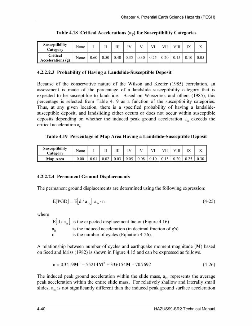
Table 4.18 Critical Accelerations (ac) for Susceptibility Categories
Susceptibility Category None I II III IV V VI VII VIII IX X
Critical Accelerations (g) None 0.60 0.50 0.40 0.35 0.30 0.25 0.20 0.15 0.10 0.05
4.2.2.2.3 Probability of Having a Landslide-Susceptible Deposit
Because of the conservative nature of the Wilson and Keefer (1985) correlation, an assessment is made of the percentage of a landslide susceptibility category that is expected to be susceptible to landslide. Based on Wieczorek and others (1985), this percentage is selected from Table 4.19 as a function of the susceptibility categories. Thus, at any given location, there is a specified probability of having a landslide-susceptible deposit, and landsliding either occurs or does not occur within susceptible deposits depending on whether the induced peak ground acceleration ais exceeds the critical acceleration ac.
Table 4.19 Percentage of Map Area Having a Landslide-Susceptible Deposit
Susceptibility Category None I II III IV V VI VII VIII IX X
Map Area 0.00 0.01 0.02 0.03 0.05 0.08 0.10 0.15 0.20 0.25 0.30
4.2.2.2.4 Permanent Ground Displacements
The permanent ground displacements are determined using the following expression:
[E PGD] = E[d / a is ] ⋅ a is ⋅ n (4-25)
where E d / a is ] is the expected displacement factor (Figure 4.16)[ ais is the induced acceleration (in decimal fraction of g's) n is the number of cycles (Equation 4-26).
A relationship between number of cycles and earthquake moment magnitude (M) based on Seed and Idriss (1982) is shown in Figure 4.15 and can be expressed as follows.
n = 0.3419M3 − 5.5214M2 + 33.6154M − 70.7692 (4-26)
The induced peak ground acceleration within the slide mass, ais, represents the average peak acceleration within the entire slide mass. For relatively shallow and laterally small slides, ais is not significantly different than the induced peak ground surface acceleration
4-40 HAZUS99-SR2 Technical Manual

Chapter 4. Potential Earth Science Hazards (PESH)
ai. For deep and large slide masses ais is less than ai. For many applications ais may be assumed equal to the accelerations predicted by the peak ground acceleration attenuation relationships being used for the loss estimation study. Considering also that topographic amplification of ground motion may also occur on hillside slopes (which is not explicitly incorporated in the attenuation relationships), the assumption of ais equal to ai may be prudent. The user may specify a ratio ais/ai less than 1.0. The default value is 1.0.
Magnitude
Num
ber o
f Cyc
les
0
5
10
15
20
25
30
5 .5 6 6.5 .5 .5 5 77 88
Figure 4.15 Relationship between Earthquake Moment Magnitude and Number of Cycles.
A relationship derived from the results of Makdisi and Seed (1978) is used to calculate downslope displacements. In this relationship, shown in Figure 4.16, the displacement factor d/ais is calculated as a function of the ratio ac/ais. For the relationship shown in Figure 4.16, the range in estimated displacement factor is shown and it is assumed that there is a uniform probability distribution of displacement factors between the upper and lower bounds.
HAZUS99-SR2 Technical Manual 4-41

Chapter 4. Potential Earth Science Hazards (PESH)
ac/ais
Dis
plac
emen
t Fac
tor,
d/ai
s (cm
/cyc
le)
0.01
0.1
1
10
100
0 0.2 0.4 0.6 0.8 1
Upper Bound
Lower Bound
Figure 4.16 Relationship between Displacement Factor and Ratio of Critical Acceleration and Induced Acceleration.
4.2.2.3 Surface Fault Rupture
4.2.2.3.1 Permanent Ground Displacements
The correlation between surface fault displacement and earthquake moment magnitude (M) developed by Wells and Coppersmith (1994) is used. The maximum displacement is given by the relationship shown in Figure 4.17. It is assumed that the maximum displacement can potentially occur at any location along the fault, although at the ends of the fault, displacements must drop to zero. The relationship developed by Wells and Coppersmith based on their empirical data set for all types of faulting (strike slip, reverse and normal) is used. It is considered that this relationship provides reasonable estimates for any type of faulting for general loss estimation purposes. The uncertainty in the maximum displacement estimate is incorporated in the loss estimation analysis. The log of the standard deviation of estimate is equal to 0.35 which is equivalent to a factor of about 2 in the displacement estimate at the plus-or-minus one standard deviation level.
The median maximum displacement (MD) is given by the following relationship:
.log(MD) = −526 + 0.79(M) (4-27)
where M is moment magnitude.
4-42 HAZUS99-SR2 Technical Manual

Chapter 4. Potential Earth Science Hazards (PESH)
Moment Magnitude
Max
Dis
plac
emen
t in
m
0.01
0.1
1
10
100
5 .5 6 .5 7 .5 8
Median
+ Std. Dev.
-Std. Dev.
5 6 7
Figure 4.17 Relationship for Estimating Maximum Surface Fault Displacement.
It has been observed that displacements along a fault vary considerably in amplitude from zero to the maximum value. Wells and Coppersmith found that the average displacement along the fault rupture segment was approximately equal to one-half the maximum displacement. This is equivalent to a uniform probability distribution for values of displacement ranging from zero to the maximum displacement. As a conservative estimate, a uniform probability distribution from one-half of the maximum fault displacement to the maximum fault displacement is incorporated in the loss estimation methodology for any location along the fault rupture.
4.2.3 Guidance for Expert-Generated Ground Failure Estimation
This section provides guidance for users who wish to use more refined methods and data to prepare improved estimates of ground failure. It is assumed that such users would be geotechnical experts with sufficient expertise in ground failure prediction to develop site-specific estimates of PGD based on regional/local data.
4.2.3.1 Input Requirements and Output Information
4.2.3.1.1 Liquefaction
Input • A map delineating areas of equal susceptibility (i.e., similar age, deposition, material
properties, and ground water depth) • Probability distribution of susceptibility variation within each area
HAZUS99-SR2 Technical Manual 4-43

Chapter 4. Potential Earth Science Hazards (PESH)
• Relationships between liquefaction probability and ground acceleration for each susceptible area
• Maps delineating topographic conditions (i.e., slope gradients and/or free-face locations) and susceptible unit thicknesses
• Relationships between ground displacements (i.e., lateral spreading and settlement), and ground acceleration for each susceptible unit, including probability distribution for displacement; they may vary within a given susceptible unit depending on topographic and liquefied zone thickness conditions
Output • Contour maps depicting liquefaction hazard and associated potential ground
displacements
4.2.3.1.2 Landsliding
Input
• A map depicting areas of equal critical or yield acceleration ac (i.e., the values of peak ground acceleration within the slide mass required to just initiate landsliding, that is, reduce the factor of safety to 1.0 at the instant of time ac occurs)
• The probability distribution for ac within each area • The ratio between induced peak ground surface acceleration, ai, and the peak ground
acceleration within the slide mass ais (note: could be a constant ratio or could vary for different areas). The value ais/ai ≤ 1. The default ratio is 1.0
• Relationships between landslide displacement d induced acceleration aic and initial or yield acceleration ac including the probability distribution for d. Different relationships can be specified for different areas. The default relationship between the displacement factor d/ais and ac/ais is shown in Figure 4.16
Output • Contour maps depicting landsliding hazard and permanent ground displacements
4.2.3.1.3 Surface Fault Rupture
Input • Predictive relationship for the maximum amount of fault displacement • Specification of regions of the fault having lower maximum displacements • Specifying other than the default relationship for the probability distribution between
minimum and maximum amounts of fault rupture displacement
Output • Amount of fault displacement at locations along the fault trace
4-44 HAZUS99-SR2 Technical Manual
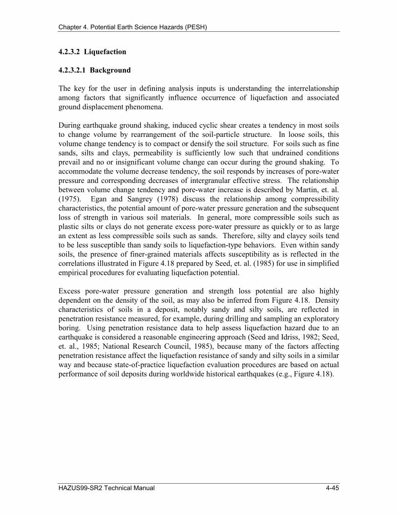
Chapter 4. Potential Earth Science Hazards (PESH)
4.2.3.2 Liquefaction
4.2.3.2.1 Background
The key for the user in defining analysis inputs is understanding the interrelationship among factors that significantly influence occurrence of liquefaction and associated ground displacement phenomena.
During earthquake ground shaking, induced cyclic shear creates a tendency in most soils to change volume by rearrangement of the soil-particle structure. In loose soils, this volume change tendency is to compact or densify the soil structure. For soils such as fine sands, silts and clays, permeability is sufficiently low such that undrained conditions prevail and no or insignificant volume change can occur during the ground shaking. To accommodate the volume decrease tendency, the soil responds by increases of pore-water pressure and corresponding decreases of intergranular effective stress. The relationship between volume change tendency and pore-water increase is described by Martin, et. al. (1975). Egan and Sangrey (1978) discuss the relationship among compressibility characteristics, the potential amount of pore-water pressure generation and the subsequent loss of strength in various soil materials. In general, more compressible soils such as plastic silts or clays do not generate excess pore-water pressure as quickly or to as large an extent as less compressible soils such as sands. Therefore, silty and clayey soils tend to be less susceptible than sandy soils to liquefaction-type behaviors. Even within sandy soils, the presence of finer-grained materials affects susceptibility as is reflected in the correlations illustrated in Figure 4.18 prepared by Seed, et. al. (1985) for use in simplified empirical procedures for evaluating liquefaction potential.
Excess pore-water pressure generation and strength loss potential are also highly dependent on the density of the soil, as may also be inferred from Figure 4.18. Density characteristics of soils in a deposit, notably sandy and silty soils, are reflected in penetration resistance measured, for example, during drilling and sampling an exploratory boring. Using penetration resistance data to help assess liquefaction hazard due to an earthquake is considered a reasonable engineering approach (Seed and Idriss, 1982; Seed, et. al., 1985; National Research Council, 1985), because many of the factors affecting penetration resistance affect the liquefaction resistance of sandy and silty soils in a similar way and because state-of-practice liquefaction evaluation procedures are based on actual performance of soil deposits during worldwide historical earthquakes (e.g., Figure 4.18).
HAZUS99-SR2 Technical Manual 4-45

Chapter 4. Potential Earth Science Hazards (PESH)
Figure 4.18 Relationship between Cyclic Stress Ratio causing Liquefaction and (N1)60 values (M=7.5) (Seed et al., 1985).
These displacement hazards are direct products of the soil behavior phenomena (i.e., high pore water pressure and significant strength reduction) produced by the liquefaction process. Lateral spreads are ground failure phenomena that occur near abrupt topographic features (i.e., free-faces) and on gently sloping ground underlain by liquefied soil. Earthquake ground-shaking affects the stability of sloping ground containing liquefiable materials by causing seismic inertia forces to be added to gravitational forces within the slope and by shaking-induced strength reductions in the liquefiable materials. Lateral spreading movements may be on the order of inches to several feet or more and are typically accompanied by surface fissures and slumping. Flow slides generally occur in
4-46 HAZUS99-SR2 Technical Manual
Chapter 4. Potential Earth Science Hazards (PESH)
liquefied materials found on steeper slopes and may involve ground movements of hundreds of feet. As a result, flowslides can be the most catastrophic of the liquefaction-related ground-failure phenomena. Fortunately, flow slides are much less common occurrences than lateral spreads.
Settlement is a result of the dissipation of excess pore pressure generated by the rearrangement of loosely compacted saturated soils into a denser configuration during shaking. Such dissipation will produce volume decreases (termed consolidation or compaction) within the soil that are manifested at the ground surface as settlement. Volume changes may occur in both liquefied and non-liquefied zones with significantly larger contributions to settlement expected to result from liquefied soil. Densification may also occur in loose unsaturated materials above the ground water table. Spatial variations in material characteristics may cause such settlements to occur differentially. Differential ground settlement may also occur near sand boil manifestations due to liquefied materials being removed from the depths of liquefaction and brought to the ground surface.
These factors have been discussed briefly in preceding sections and incorporated to the extent possible in characterizing relationships of Section 4.2.2.1. The challenge to the user is to translate regional/local data, experience and judgment into defining site-specific relationships. The following paragraphs offer additional comments regarding various aspects of that process.
4.2.3.2.2 Susceptibility
Fundamental soil characteristics and physical processes that affect liquefaction susceptibility have been identified through case histories and laboratory studies. Depositional environments of sediments and their geologic ages control these characteristics and processes, as discussed by Youd and Perkins (1978).
The depositional environments of sediments control grain size distribution and, in part, the relative density and structural arrangement of grains. Grain size characteristics of a soil influence its susceptibility to liquefaction. Fine sands tend to be more susceptible than silts and gravels. All cohesionless soils, however, may be considered potentially liquefiable as the influence of particle size distribution is not thoroughly understood. In general, cohesive soils that contain more than about 20 percent clay may be considered nonliquefiable (Seed and Idriss, 1982, present criteria for classifying a soil as nonliquefiable).
Relative density and structural arrangement of grains (soil structure) greatly influence liquefaction susceptibility of a cohesionless soil. Soils that have higher relative densities and more stable soil structure have a lower susceptibility to liquefaction. These factors may be related to both depositional environment and age. Sediments undisturbed after deposition (e.g., lagoon or bay deposits) tend to have lower densities and less stable structures than sediments subjected to wave or current action. With increasing age of a
HAZUS99-SR2 Technical Manual 4-47

Chapter 4. Potential Earth Science Hazards (PESH)
deposit, relative density may increase as particles gradually work closer together. The soil structure also may become more stable with age through slight particle reorientation or cementation. Also, the thickness of overburden sediments may increase with age, and the increased pressures associated with a thicker overburden will tend to increase the density of the soil deposit.
An increase in the ratio of effective lateral earth pressure to effective vertical or overburden earth pressure in a soil has been shown to reduce its liquefaction susceptibility. Such an increase will occur when overburden is removed by erosion.
In general, it is thought that the soil characteristics and processes that result in a lower liquefaction susceptibility also result in higher penetration resistance when a soil sampler is driven into a soil deposit. Therefore, blow count values, which measure penetration resistance of a soil sampler in a boring, are a useful indicator of liquefaction susceptibility. Similarly, the resistance from pushing a cone penetrometer into the soil is a useful indicator of liquefaction susceptibility. An understanding of the depositional environments and ages of soil units together with penetration resistance data enables assessment of liquefaction susceptibility.
Additional information helpful to enhancing/refining the susceptibility characterization is observation of liquefaction and related phenomena during historical earthquakes, as well as evidence of paleoliquefaction. Although such information does not exist for all locations and its absence does not preclude liquefaction susceptibility, it is available for numerous locations throughout the country; for example, in Northern California (Youd and Hoose, 1978; Tinsley, et. al., 1994); in the New Madrid region (Obermeier, 1989; Wesnousky, et. al., 1989); in the Charleston, South Carolina region (Obermeier, et. al., 1986; Gohn, et. al., 1984), in the northeastern United States (Tuttle and Seeber, 1989); among other locales. Incorporation of such historical information has been shown to significantly enhance liquefaction-related loss estimation predictions (Geomatrix, 1993).
4.2.3.2.3 Liquefaction Probability
As described previously, simplified procedures for evaluating liquefaction potential presented by Seed, et. al. (1985), as well as probabilistic approach presented by Liao, et. al. (1988), are useful tools for helping to characterize the relationships among liquefaction probability, peak ground acceleration, duration of shaking (magnitude), and groundwater depth, etc. A parameter commonly utilized in these procedures is penetration resistance, which was previously discussed relative to susceptibility. Within a given geologic unit, experience indicates that subsurface investigations may obtain a certain scatter in penetration resistance without necessarily any observable trend for variation horizontally or vertically within that unit. In such cases, a single representative penetration resistance value is often selected for evaluating the liquefaction potential at the site. The representative value is very much site-specific and depends on the particular distribution of penetration resistance values measured. For example, if most of the values are very close to each other, with a few much higher or lower values, the representative
4-48 HAZUS99-SR2 Technical Manual
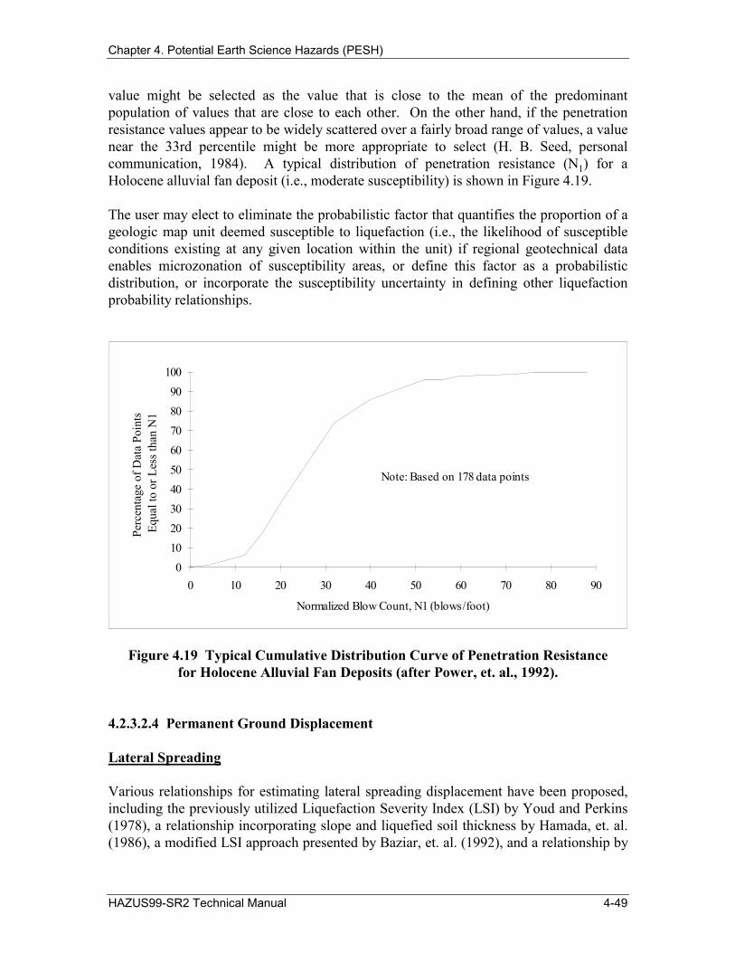
Chapter 4. Potential Earth Science Hazards (PESH)
value might be selected as the value that is close to the mean of the predominant population of values that are close to each other. On the other hand, if the penetration resistance values appear to be widely scattered over a fairly broad range of values, a value near the 33rd percentile might be more appropriate to select (H. B. Seed, personal communication, 1984). A typical distribution of penetration resistance (N1) for a Holocene alluvial fan deposit (i.e., moderate susceptibility) is shown in Figure 4.19.
The user may elect to eliminate the probabilistic factor that quantifies the proportion of a geologic map unit deemed susceptible to liquefaction (i.e., the likelihood of susceptible conditions existing at any given location within the unit) if regional geotechnical data enables microzonation of susceptibility areas, or define this factor as a probabilistic distribution, or incorporate the susceptibility uncertainty in defining other liquefaction probability relationships.
Normalized Blow Count, N1 (blows/foot)
Perc
enta
ge o
f Dat
a Po
ints
Eq
ual t
o or
Les
s tha
n N
1
0 10 20 30 40 50 60 70 80 90
100
0 10 0 30 0 0 60 0 0 90
Note: Based on 178 data points
2 4 5 7 8
Figure 4.19 Typical Cumulative Distribution Curve of Penetration Resistance for Holocene Alluvial Fan Deposits (after Power, et. al., 1992).
4.2.3.2.4 Permanent Ground Displacement
Lateral Spreading
Various relationships for estimating lateral spreading displacement have been proposed, including the previously utilized Liquefaction Severity Index (LSI) by Youd and Perkins (1978), a relationship incorporating slope and liquefied soil thickness by Hamada, et. al. (1986), a modified LSI approach presented by Baziar, et. al. (1992), and a relationship by
HAZUS99-SR2 Technical Manual 4-49
Chapter 4. Potential Earth Science Hazards (PESH)
Bartlet and Youd (1992), in which they characterize displacement potential as a function of global earthquake and local site characteristics (e.g., slope, liquefaction thickness, and grain size distribution). Relationships that are more site-specific may be developed based on simple stability and deformation analysis for lateral spreading conditions using undrained residual strengths for liquefied sand (Seed and Harder, 1990) along with Newmark-type (1965) and Makdisi and Seed (1978) displacement approaches. To reasonably represent the lateral spreading hazard by either published relationships or area-specific analyses, generalized information regarding stratigraphic conditions (i.e., depth to and thickness of the liquefied zone) and topographic conditions (i.e., ground slope and free-face situations) are required.
Ground Settlement
Relationships for assessing ground settlement are available (e.g., Tokimatsu and Seed, 1978; Ishihara, 1991) and are suggested to the user for guidance. In addition, test results presented by Lee and Albaisa (1974) suggest that the magnitude of volumetric strain following liquefaction may be dependent on grain-size distribution. Area-specific information required for developing settlement relationships is similar to that for lateral spreading.
4.2.3.3 Landsliding
4.2.3.3.1 Background
The key assessment is the generation of a map denoting areas of equal landslide susceptibility and their corresponding values of critical acceleration. This should be accomplished considering the geographical distribution of facilities at risk in the region and the types of landsliding that could affect the facilities.
4.2.3.3.2 Landslide Susceptibility
Keefer (1984) and Wilson and Keefer (1985) have identified many different types of landsliding, ranging from rock falls to deep-seated coherent soil or rock slumps to soil lateral spreads and flows. For loss estimation purposes, the potential for lateral spreads and flows should be part of the liquefaction potential assessment rather than the landslide potential. The significance of other forms of downslope movement depends on the potential for such movements to damage facilities. The emphasis on characterizing landslide susceptibility should be on failure modes and locations that pose a significant risk to facilities. For example, if the potential for rock falls were high (because of steep terrain and weak rock) but could occur only in undeveloped areas, then it would not be important to characterize the critical acceleration for this mode of failure. As another example, in evaluating the probability of landsliding and the amount of displacements as part of a regional damage assessment for a utility district (Power and others, 1994), it was assessed that two types of landsliding posed the major risk to the facilities and piping: activation of existing deep-seated landslide deposits that had been mapped in hillside
4-50 HAZUS99-SR2 Technical Manual

Chapter 4. Potential Earth Science Hazards (PESH)
areas and that had the potential for disrupting areas in which water lines were located (landslides often covering many square blocks); and local slumping of roadway sidehill fills in which water lines were embedded.
Having identified the modes and geographic areas of potential landsliding of significance, critical acceleration can be evaluated for these modes and areas. It is not necessarily required to estimate ac as a function of slope angle. In some cases, it may be satisfactory to estimate ac and corresponding ranges of values for generalized types of landslides and subregions, for example, reactivation of existing landslides within a certain subregion or within the total region. However, it is usually necessary to distinguish between dry and wet conditions because ac is usually strongly dependent on groundwater conditions.
In general, there are two approaches to estimating ac: an empirical approach utilizing observations of landsliding in past earthquakes and corresponding records or estimates of ground acceleration; and an analytical approach, in which values of a
c are calculated by
pseudo-static slope stability analysis methods. Often, both approaches may be utilized (e.g., Power, et. al., 1994). When using the analytical approach, the sensitivity of results to soil strength parameters must be recognized. In assessing strength parameter values and ranges, it is often useful to back-estimate values, which are operable during static conditions. Thus, for certain types of geology, slope angles, static performance observations during dry and wet seasons, and estimates of static factors of safety, it may be possible to infer reasonable ranges of strength parameters from static slope stability analyses. For earthquake loading conditions, an assessment should also be made as to whether the short-term dynamic, cyclic strength would differ from the static strength. If the soil or rock is not susceptible to strength degradation due to cyclic load applications or large deformations, then it may be appropriate to assign strength values higher than static values due to rate of loading effects. On the other hand, values even lower than static values may be appropriate if significant reduction in strength is expected (such as due to large-deformation-induced remolding of soil).
4.2.3.3.3 Probability of Landsliding
The probability of landsliding at any location is determined by comparing the induced peak ground acceleration (adjusted to the value of the peak acceleration in the landslide mass ais) with the assessed distribution for critical acceleration ac (Figure 4.20).
4.2.3.3.4 Permanent Ground Displacements
In assessing soil deformations using relationships such as shown in Figure 4.16, it should be kept in mind that the relationships are applicable to slope masses that exhibit essentially constant critical accelerations. For cases where significant reduction in strength may occur during the slope deformation process, these relationships may significantly underestimate deformations if the peak strength values are used. For example, deformations cannot be adequately estimated using these simplified correlations
HAZUS99-SR2 Technical Manual 4-51

Chapter 4. Potential Earth Science Hazards (PESH)
in cases of sudden, brittle failure, such as rock falls or soil or rock avalanches on steep slopes.
4.2.3.4 Surface Fault Rupture
4.2.3.4.1 Permanent Ground Displacements
Refinements or alternatives that an expert may wish to consider in assessing displacements associated with surface fault rupture include: a predictive relationship for maximum fault displacement different from the default relationship (Figure 4.17), specification of regions of the fault rupture (near the ends) where the maximum fault displacement is constrained to lower values, and specification of other than the default relationship for the probability distribution of fault rupture between minimum and maximum values.
Acceleration
ac1 a is ac2
Prob
abili
ty D
ensi
ty fo
r ac
Figure 4.20 Evaluation of Probability of Landsliding.
4-52 HAZUS99-SR2 Technical Manual
Chapter 4. Potential Earth Science Hazards (PESH)
4.3 References
Algermissen, S. T., et. al., 1982. "Probabilistic Estimates of Maximum Acceleration and Velocity in Rock in the Contiguous United States", USGS Open File Report 82-1033, United States Geological Survey.
Association of Bay Area Governments (ABAG), 1980. "Liquefaction Potential and Liquefaction Susceptibility Maps", San Francisco Bay region, original scale 1:250,000.
Atkinson G. M. and Boore D. M., 1995. “Ground-Motion Relations for Eastern North America”, Bulletin of the Seismological Society of America, vol. 85, No. 1, February, pp. 17-30.
Bartlett, S. F., and Youd, T. L., 1992. "Empirical Prediction of Lateral Spread Displacement", in Hamada, M., and O'Rourke, T. D. (eds.), Proceedings from the Fourth Japan-U.S. Workshop on Earthquake Resistant Design of Lifeline Facilities and Countermeasures for Soil Liquefaction, Technical Report NCEER-92-0019, v. I, pp. 351-365.
Boore, D. M., Joyner, W. B., and Fumal, T. E., 1993. "Estimation of Response Spectra and Peak Acceleration from Western North American Earthquakes: An Interim Report", USGS Open File Report 93-509, Menlo Park, California, United States Geological Survey.
Boore, D. M., Joyner, W. B., and Fumal, T. E., 1994a. "Estimation of Response Spectra and Peak Acceleration from Western North American Earthquakes: An Interim Report, Part 2", USGS Open File Report 94-127, Menlo Park, California, United States Geological Survey.
Boore, D. M., Joyner, W. B., and Fumal, T. E., 1994b. "Ground Motion Estimates for Strike- and Reverse-Slip Faults", (preprint).
Borcherdt, R. D. 1994. "New Developments in Estimating Site Response Effects on Ground Motion", Proceeding of Seminar on New Developments in Earthquake Ground Motion Estimation and Implications for Engineering Design Practice ATC-35, Applied Technology Council, Redwood City, California.
Campbell, K. W., and Bozorgnia, Y., 1994. "Near-Source Attenuation of Peak Horizontal Acceleration from Worldwide Accelerograms Recorded from 1957 to 1993", Proceedings, Fifth U.S. National Conference on Earthquake Engineering, Chicago, Illinois, July 10-14: v III, pp. 283-292.
Egan, J. A., and Sangrey, D. A., 1978. "Critical State Model for Cyclic Load Pore Pressure", Proceedings, Earthquake Engineering and Soil Dynamics Conference and Exhibit, Pasadena, California, June 19-21.
HAZUS99-SR2 Technical Manual 4-53
Chapter 4. Potential Earth Science Hazards (PESH)
Federal Emergency Management Agency, 1992. "FEMA 178 - NEHRP Handbook for the Seismic Evaluation of Existing Buildings", Washington, D. C., Developed by the Building Seismic Safety Council (BSSC) for the Federal Emergency Management Agency (FEMA).
Federal Emergency Management Agency, 1995. FEMA 222A and 223A - NEHRP Recommended Provisions for Seismic Regulations for New Buildings, 1994 Edition, Washington, D. C., Developed by the Building Seismic Safety Council (BSSC) for the Federal Emergency Management Agency (FEMA).
Federal Emergency Management Agency, 1997. 1997 NEHRP Recommended Provisions for Seismic Regulations for New Buildings, (in press) Washington, D. C., Developed by the Building Seismic Safety Council (BSSC) for the Federal Emergency Management Agency (FEMA).
Frankel, A., Mueller, C., Barnhard, T. , Perkins, D., Leyendecker, E. V., Dickman, N., Hanson, S. and M. Hopper, 1996. National Seismic-Hazard Maps: Documentation June 1996, USGS Open-File Report 96-532: United States Geological Survey.
Frankel, A., 1997. Issues and Assumptions for Draft Alaska Seismic Hazard Maps, United States Geological Survey, Golden, CO.
Goodman, R. E., and Seed, H. B., 1966. "Earthquake-Induced Displacements in Sand Embankments", Journal of the Soil Mechanics and Foundations Division, Proceedings of the American Society of Civil Engineers, vol. 92, no. SM2, pp. 125-146.
Global Hypocenter Database, Version 2.0, 1992. United States Geological Survey, National Earthquake Information Center, Denver, Colorado.
Grant, W. P., W. J. Perkins, and T. L. Youd. 1991. Evaluation of Liquefaction Potential in Seattle, Washington - USGS Professional Paper 91-0441T: United States Geological Survey.
Joyner, W. B., and Boore, D. M., 1988. "Measurement, Characterization, and Prediction of Strong Ground Motion", Proceedings of Earthquake Engineering & Soil Dynamics II, pp. 43- 102. Park City, Utah, 27 June 1988. New York: Geotechnical Division of the American Society of Civil Engineers.
Keefer, D. K.,1984. "Landslides Caused by Earthquakes", Geological Society of America Bulletin, vol. 95, pp. 406-421.
Klein, F., Frankel, A., Mueller, C., Wesson, R., and P. Okubo, 1998. Documentation for Draft Seimic-Hazard Maps for the State of Hawaii, United States Geological Survey.
4-54 HAZUS99-SR2 Technical Manual

Chapter 4. Potential Earth Science Hazards (PESH)
Lee, K. L., and Albaisa, A., 1974. "Earthquake Induced Settlement in Saturated Sands", Journal of the Soil Mechanics and Foundation Division, ASCE 100(GTA), pp. 387-406.
Leyendecker, E.V., and Frankel, A., 1998. Dipping Fault Attenuation Relations used in Developing 1996 USGS Probabilistic Maps, Report to the National Institute of Building Sciences, November, 1998.
Liao, S. S., Veneziano, D., and Whitman, R. V., 1988. "Regression Models for Evaluating Liquefaction Probability", Journal of Geotechnical Engineering, vol. 114, No. 4, April.
Makdisi, F. I. and Seed, H. B., 1978. "Simplified Procedure for Estimating Dam and Embankment Earthquake-Induced Deformations", Journal of the Geotechnical Engineering Division, American Society of Civil Engineers, vol. 104, No. GT7, July, pp. 849-867.
Martin G. R., Finn, W. D. L., and Seed, H. B., 1975. "Fundamentals of Liquefaction Under Cyclic Loading", Journal of the Geotechnical Engineering Division, ASCE 104(GT5), pp. 423-438.
Munson, Clifford G., and Thurber, Clifford H., 1997. "Analysis of the Attenuation of Strong Ground Motion on the Island of Hawaii", Bulletin of the Seismological Society of America, vol. 87, No. 4, August, pp. 945-960.
National Research Council, 1985, "Liquefaction of Soils During Earthquakes", Committee on Earthquake Engineering, Commission on Engineering and Technical Systems, National Academy Press, Washington, DC.
Newmark, N. M., 1965. "Effects of Earthquakes on Dams and Embankments", Geotechnique, vol. 15, no. 2, pp. 139-160.
Newmark, N. M. and Hall, W. J., 1982. “Earthquake Spectra and Design”, EERI Monograph.
Power, M. S., A. W. Dawson, D. W. Streiff, R. G. Perman, and S. C. Haley, 1982. Evaluation of Liquefaction Susceptibility in the San Diego, California Urban Area. Proceedings 3rd International Conference on Microzonation, II, pp. 957-968.
Power, M. S., R. G. Perman, J. R. Wesling, R. R. Youngs, M. K. Shimamoto, 1991. Assessment of Liquefaction Potential in the San Jose, California Urban Area. Proceedings 4th International Conference on Microzonation, II, pp. 677-684, Stanford, CA.
HAZUS99-SR2 Technical Manual 4-55

Chapter 4. Potential Earth Science Hazards (PESH)
Power, M. S., Taylor, C. L., and Perman, R. C., 1994. "Evaluation of Regional Landsliding Hazard Potential for Utility District - Eastern San Francisco Bay Area", Proceedings of the U.S. Fifth National Conference on Earthquake Engineering, Chicago, Illinois, July .
Sadigh, K., Chang C.-Y., Abrahamson, N. A., Chiou, S. J. and M. S. Power, 1993. “Specification of Long-Period Ground Motions: Updated Attenuation Relationships for Rock Site Conditions and Adjustment Factors for Near-Fault Effects”, Proceedings of ATC 17-1 Seminar on Seismic isolation, Passive Energy Dissipation, and Active Control, Applied Technology Council, Redwood City, CA, pp. 59-70.
Sadigh, K., Egan, J. A., and Youngs, R. R., 1986. "Specification of Ground Motion for Seismic Design of Long Period Structures", Earthquake Notes, vol. 57, no. 1, p. 13, relationships are tabulated in Joyner and Boore (1988) and Youngs and others (1987).
Sayv, Jean, 1998. "Ground Motion Attenuation in the Eastern North America", Lawerence Livermore National Laboratory, Livermore, CA.
Seed, R. B., and Harder, L. F., 1990. "SPT-Based Analysis of Cyclic Pore Pressure Generation and Undrained Residual Strength", Proceedings of the H. B. Seed Memorial Symposium, vol. 2, pp. 351-376.
Seed, H. B., and Idriss, I. M., 1971. "Simplified Procedure for Evaluating Soil Liquefaction Potential", Journal of the Soil Mechanics and Foundations Division, ASCE, vol. 97, no. SM9, Proceedings Paper 8371, September, pp. 1249-1273.
Seed, H. B., and Idriss, I. M. 1982. "Ground Motions and Soil Liquefaction During Earthquakes", Earthquake Engineering Research Institute, Oakland, California, Monograph Series, p. 13.
Seed, H. B., Tokimatsu, K., Harder, L. F., and Chung, R. M., 1985. "Influence of SPT Procedures in Soil Liquefaction Resistance Evaluations, Journal of Geotechnical Engineering, American Society of Civil Engineers, , vol. 111, no. 12, p. 1425-1445.
Tinsley, J. C., T. L. Youd, D. M. Perkins, and A. T. F. Chen, 1985. Evaluating Liquefaction Potential, Evaluating Earthquake Hazards in the Los Angeles Region -USGS Professional Paper 1360. pp. 263-316.
Tokimatsu, A. M., and Seed, H. B., 1987. "Evaluation of Settlements in Sands Due to Earthquake Shaking", Journal of the Geotechnical Division, American Society of Civil Engineers, vol. 113, no. 8, pp. 681-878.
Toro, G. R., Abrahamson, N. A. and Schneider, J. F., 1997. “Engineering Model of Strong Ground Motions from Earthquakes in the Central and Eastern United States”, Seismological Research Letters, January/February.
4-56 HAZUS99-SR2 Technical Manual
Chapter 4. Potential Earth Science Hazards (PESH)
Toro, G. R. and McGuire, R. K., 1991. “Evaluations of Seismic Hazard at the Paducah Gaseous Diffusion Plant”, Third DOE Natural Phenomena Hazards Mitigation Conference, pp. 157-165.
Updike, R. G., Egan, J. A., Moriwaki, Y., Idriss, I. M., and Moses, T. L., 1988, "A Model for Earthquake-Induced Translatory Landslides in Quaternary Sediments", Geological Society of America Bulletin, vol. 100, May, pp. 783-792.
Wells, D. L. and Coppersmith, K. J., 1994. "New Empirical Relationships Among Magnitude, Rupture Length, Rupture Width, and Surface Displacement", Bulletin of the Seismological Society of America, v 84, pp. 974-1002.
Wieczorek, G. F., Wilson, R. C. and Harp, E. L., 1985. "Map of Slope Stability During Earthquakes in San Mateo County, California", U.S. Geological Survey Miscellaneous Investigations Map I-1257-E, scale 1:62,500.
Wilson, R. C., and Keefer D. K., 1985. "Predicting Areal Limits of Earthquake Induced Landsliding, Evaluating Earthquake Hazards in the Los Angeles Region", U.S. Geological Survey Professional Paper, Ziony, J. I., Editor, pp. 317-493.
Youd, T. L., and Hoose, S. N., 1978. "Historic Ground Failures in Northern California Triggered by Earthquakes", U.S. Geological Survey Professional Paper 993, 177 p.
Youd, T. L., and Perkins, D. M., 1978. "Mapping of Liquefaction Induced Ground Failure Potential", Journal of the Geotechnical Engineering Division, American Society of Civil Engineers, vol. 104, no. 4, pp. 433-446.
Youd, T. L., and Perkins, D. M., 1987. "Mapping of Liquefaction Severity Index", Journal of the Geotechnical Engineering Division, American Society of Civil Engineers, vol. 118, no. 11, pp. 1374-1392.
Youngs R. R., Chiou, S. J., Silva W. L., and Humphrey J. R., 1997. "Strong Ground Motion Attenuation Relationships for Subduction Zone Earthquakes", Seismological Research Letters, January/February.
HAZUS99-SR2 Technical Manual 4-57

Chapter 4. Potential Earth Science Hazards (PESH)
Appendix 4A Tables of Attenuation Values for the Eastern U.S. Attenuation
Relationships
This appendix gives tabular results for the default Eastern United States attenuation relationships used in the methodology. Each table gives the peak ground or spectral values in relationship to hypocentral distance (km) and moment magnitude (M). The units for the peak ground acceleration and spectral acceleration are fraction of gravity and the peak ground velocity values are in centimeters per second. In these tables, hypocentral distance is used in Frankel et al., and closest horizontal distance is used in Toro et al. The index of the appendix is as follows:
Frankel et al. (1996)
Table 4A.1 Peak Ground Acceleration Values 4A-2 Table 4A.2 Peak Ground Velocity Values 4A-2 Table 4A.3 Spectral Acceleration Values (T=0.20 sec) 4A-3 Table 4A.4 Spectral Acceleration Values (T=0.30 sec) 4A-3 Table 4A.5 Spectral Acceleration Values (T=1.00 sec) 4A-5
Toro et al. (1997)
Table 4A.6 Peak Ground Acceleration Values 4A-7 Table 4A.7 Spectral Acceleration Values (T=0.20 sec) 4A-8 Table 4A.8 Spectral Acceleration Values (T=0.30 sec) 4A-8 Table 4A.9 Spectral Acceleration Values (T=1.00 sec) 4A-10
4-58 HAZUS99-SR2 Technical Manual

Chapter 4. Potential Earth Science Hazards (PESH)
HAZUS99-SR2 Technical Manual 4-59
Table 4A.1: eak Ground Acceleration Attenuation Values (in units of g) Distance oment Magnitude
(km) 5.0 7.0 10 0.36 0.56 0.85 1.23 1.50* 1.50* 1.50* 20 0.14 0.79 1.50* 30 0.08 0.49 40 0.05 0.33 50 0.04 0.24 60 0.03 0.19 70 0.02 0.16 80 0.02 0.14 90 0.02 0.13
100 0.01 0.12 120 0.01 0.10 140 0.01 0.09 160 0.01 0.07 180 0.01 0.06 200 0.01 0.05 250 0.00 0.04 300 0.00 0.03 350 0.00 0.02
* PGA capped at 1.5g
Table 4A.2: Peak Ground Velocity Attenuation Values (cm/sec) Distance oment Magnitude
(km) 5.0 7.0 8.0 10 7.4 14.4 81.3 145.5 257.0 20 3.2 6.4 12.0 39.8 125.9 30 1.9 14.1 25.7 46.0 82.6 40 1.3 18.1 33.6 60.0 50 0.9 14.2 26.0 46.9 60 0.7 11.5 21.3 38.8 70 0.6 10.0 18.8 34.3 80 0.5 9.1 17.3 31.6 90 0.5 8.8 16.9 31.3
100 0.4 8.5 16.5 30.9 120 0.4 8.1 15.8 29.8 140 0.3 7.4 14.6 27.9 160 0.3 6.6 13.2 25.5 180 0.3 6.0 12.0 23.4 200 0.2 5.4 10.8 21.3 250 0.2 4.3 17.9 300 0.1 3.5 15.5 350 0.1 3.0 13.6
PM
6.5 6.0 5.5 8.0 7.5
0.56 0.37 0.24 1.15 0.33 0.22 0.14 1.01 0.71 0.22 0.14 0.09 0.69 0.48 0.16 0.10 0.06 0.51 0.36 0.12 0.08 0.05 0.41 0.28 0.10 0.06 0.04 0.34 0.23 0.09 0.05 0.03 0.29 0.21 0.08 0.05 0.03 0.28 0.19 0.07 0.05 0.03 0.26 0.18 0.06 0.04 0.02 0.23 0.16 0.05 0.03 0.02 0.20 0.14 0.04 0.03 0.02 0.17 0.11 0.04 0.02 0.01 0.15 0.10 0.03 0.02 0.01 0.13 0.08 0.02 0.01 0.01 0.09 0.06 0.02 0.01 0.00 0.07 0.04 0.01 0.01 0.00 0.05 0.03
M6.5 6.0 5.5 7.5
47.1 26.3 22.0 71.3
7.5 3.9 9.9 5.2 2.6 7.6 3.9 2.0 6.1 3.1 1.5 5.2 2.7 1.3 4.7 2.3 1.1 4.6 2.2 1.1 4.4 2.1 1.0 4.1 2.0 0.9 3.7 1.7 0.8 3.2 1.5 0.7 2.9 1.3 0.6 2.6 1.2 0.5 2.0 0.9 0.4 9.0 1.6 0.7 0.3 7.7 1.4 0.6 0.2 6.6
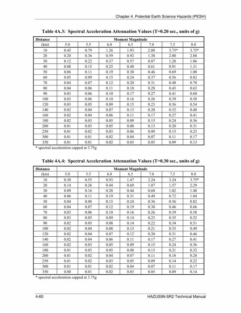
Chapter 4. Potential Earth Science Hazards (PESH)
4-60 HAZUS99-SR2 Technical Manual
Table 4A.3: pectral Acceleration Attenuation Values (T=0.20 sec., units of g) Distance oment Magnitude
(km) 5.0 7.0 10 0.45 0.79 1.26 1.93 2.88 3.75* 3.75* 20 0.20 1.38 30 0.12 0.87 40 0.08 0.61 50 0.06 0.46 60 0.05 0.37 70 0.04 0.31 80 0.04 0.28 90 0.03 0.27
100 0.03 0.26 120 0.03 0.23 140 0.02 0.20 160 0.02 0.17 180 0.02 0.15 200 0.01 0.13 250 0.01 0.09 300 0.01 0.07 350 0.01 0.05
* spectral acceleration capped at 3.75g
Table 4A.4: pectral Acceleration Attenuation Values (T=0.30 sec., units of g) Distance oment Magnitude
(km) 5.0 7.0 10 0.30 2.24 3.75* 20 0.14 1.07 30 0.09 0.68 40 0.06 0.49 50 0.04 0.36 60 0.04 0.30 70 0.03 0.26 80 0.03 0.23 90 0.02 0.22
100 0.02 0.21 120 0.02 0.20 140 0.02 0.17 160 0.02 0.15 180 0.01 0.13 200 0.01 0.11 250 0.01 0.09 300 0.01 0.07 350 0.00 0.05
* spectral acceleration capped at 3.75g
SM
6.5 6.0 5.5 8.0 7.5
0.92 0.59 0.36 2.88 2.00 0.57 0.37 0.22 1.86 1.28 0.40 0.25 0.15 1.31 0.91 0.30 0.19 0.11 1.00 0.69 0.24 0.15 0.09 0.82 0.56 0.20 0.12 0.07 0.70 0.48 0.18 0.11 0.06 0.63 0.43 0.17 0.10 0.06 0.60 0.41 0.16 0.10 0.06 0.58 0.39 0.15 0.09 0.05 0.54 0.36 0.13 0.07 0.04 0.48 0.32 0.11 0.06 0.04 0.41 0.27 0.09 0.05 0.03 0.36 0.24 0.08 0.05 0.03 0.31 0.20 0.06 0.03 0.02 0.23 0.15 0.04 0.02 0.01 0.17 0.11 0.03 0.02 0.01 0.13 0.09
SM
6.5 6.0 5.5 8.0 7.5 1.47 0.93 0.55 3.24 0.69 0.44 0.26 2.29 1.57 0.44 0.28 0.16 1.48 1.02 0.31 0.19 0.11 1.04 0.72 0.24 0.15 0.08 0.82 0.56 0.19 0.12 0.07 0.66 0.46 0.16 0.10 0.06 0.58 0.39 0.14 0.09 0.05 0.52 0.35 0.14 0.08 0.05 0.51 0.34 0.13 0.08 0.04 0.49 0.33 0.12 0.07 0.04 0.46 0.31 0.11 0.06 0.04 0.41 0.27 0.09 0.05 0.03 0.36 0.24 0.08 0.05 0.03 0.32 0.21 0.07 0.04 0.02 0.28 0.18 0.05 0.03 0.02 0.22 0.14 0.04 0.02 0.01 0.17 0.11 0.03 0.02 0.01 0.14 0.09

Chapter 4. Potential Earth Science Hazards (PESH)
Table 4A.5: Spectral Acceleration Attenuation Values (T=1.00 sec., units of g) Distance Moment Magnitude
(km) 5.0 5.5 6.0 6.5 7.0 7.5 8.0 10 0.03 0.09 0.22 0.42 0.71 1.11 1.70 20 0.02 0.05 0.11 0.21 0.35 0.55 0.83 30 0.01 0.03 0.07 0.13 0.22 0.36 0.55 40 0.01 0.02 0.05 0.10 0.17 0.26 0.40 50 0.01 0.02 0.04 0.07 0.13 0.21 0.31 60 0.00 0.01 0.03 0.06 0.10 0.17 0.26 70 0.00 0.01 0.03 0.05 0.09 0.15 0.23 80 0.00 0.01 0.03 0.05 0.09 0.14 0.21 90 0.00 0.01 0.03 0.05 0.08 0.13 0.21
100 0.00 0.01 0.02 0.05 0.08 0.13 0.20 120 0.00 0.01 0.02 0.04 0.08 0.13 0.20 140 0.00 0.01 0.02 0.04 0.07 0.12 0.18 160 0.00 0.01 0.02 0.04 0.06 0.10 0.16 180 0.00 0.01 0.02 0.03 0.06 0.10 0.15 200 0.00 0.01 0.02 0.03 0.05 0.09 0.13 250 0.00 0.01 0.01 0.02 0.04 0.07 0.11 300 0.00 0.00 0.01 0.02 0.03 0.06 0.09 350 0.00 0.00 0.01 0.02 0.03 0.05 0.08
HAZUS99-SR2 Technical Manual 4-61

Chapter 4. Potential Earth Science Hazards (PESH)
Attenuation Values Based on Toro, Abrahamson and Schneider
Table 4A.6: Peak Ground Acceleration Attenuation Values (in units of g) Distance Moment Magnitude
(km) 5.0 5.5 6.0 6.5 7.0 7.5 8.0 0 0.28 0.39 0.54 0.72 0.94 1.19 1.47
10 0.18 0.26 0.36 0.50 0.68 0.89 1.13 20 0.10 0.15 0.21 0.30 0.42 0.58 0.77 30 0.07 0.10 0.14 0.20 0.29 0.40 0.55 40 0.05 0.07 0.10 0.15 0.21 0.30 0.41 50 0.04 0.05 0.08 0.11 0.16 0.23 0.32 60 0.03 0.04 0.06 0.09 0.13 0.19 0.26 70 0.02 0.03 0.05 0.07 0.11 0.15 0.22 80 0.02 0.03 0.04 0.06 0.09 0.13 0.19 90 0.02 0.02 0.04 0.05 0.08 0.11 0.16
100 0.01 0.02 0.03 0.05 0.07 0.10 0.14 120 0.01 0.02 0.02 0.04 0.05 0.08 0.11 140 0.01 0.01 0.02 0.03 0.04 0.06 0.09 160 0.01 0.01 0.02 0.02 0.03 0.05 0.07 180 0.01 0.01 0.01 0.02 0.03 0.04 0.06 200 0.01 0.01 0.01 0.02 0.02 0.04 0.05 250 0.00 0.01 0.01 0.01 0.02 0.03 0.04 300 0.00 0.00 0.01 0.01 0.01 0.02 0.03 350 0.00 0.00 0.00 0.01 0.01 0.01 0.02
4-62 HAZUS99-SR2 Technical Manual

Chapter 4. Potential Earth Science Hazards (PESH)
Table 4A.7: Spectral Acceleration Attenuation Values (T=0.20 sec., units of g) Distance Moment Magnitude
(km) 5.0 5.5 6.0 6.5 7.0 7.5 8.0 0 0.46 0.66 0.93 1.27 1.70 2.23 2.85
10 0.30 0.43 0.62 0.88 1.22 1.66 2.21 20 0.18 0.26 0.39 0.56 0.80 1.13 1.55 30 0.12 0.18 0.27 0.40 0.57 0.82 1.15 40 0.09 0.14 0.20 0.30 0.44 0.63 0.90 50 0.07 0.11 0.16 0.24 0.35 0.51 0.73 60 0.06 0.09 0.13 0.19 0.28 0.42 0.60 70 0.05 0.07 0.11 0.16 0.24 0.35 0.51 80 0.04 0.06 0.09 0.14 0.20 0.30 0.44 90 0.03 0.05 0.08 0.12 0.17 0.26 0.38
100 0.03 0.05 0.07 0.10 0.16 0.23 0.34 120 0.02 0.04 0.06 0.08 0.13 0.19 0.28 140 0.02 0.03 0.05 0.07 0.11 0.16 0.24 160 0.02 0.03 0.04 0.06 0.09 0.13 0.20 180 0.01 0.02 0.03 0.05 0.08 0.11 0.17 200 0.01 0.02 0.03 0.04 0.07 0.10 0.15 250 0.01 0.01 0.02 0.03 0.05 0.07 0.10 300 0.01 0.01 0.01 0.02 0.03 0.05 0.07 350 0.00 0.01 0.01 0.02 0.02 0.04 0.05
HAZUS99-SR2 Technical Manual 4-63
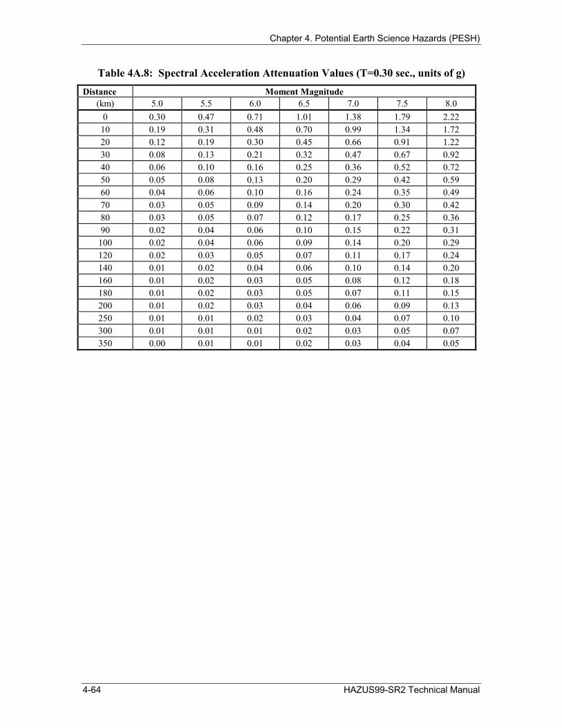
Chapter 4. Potential Earth Science Hazards (PESH)
Table 4A.8: Spectral Acceleration Attenuation Values (T=0.30 sec., units of g) Distance Moment Magnitude
(km) 5.0 5.5 6.0 6.5 7.0 7.5 8.0 0 0.30 0.47 0.71 1.01 1.38 1.79 2.22
10 0.19 0.31 0.48 0.70 0.99 1.34 1.72 20 0.12 0.19 0.30 0.45 0.66 0.91 1.22 30 0.08 0.13 0.21 0.32 0.47 0.67 0.92 40 0.06 0.10 0.16 0.25 0.36 0.52 0.72 50 0.05 0.08 0.13 0.20 0.29 0.42 0.59 60 0.04 0.06 0.10 0.16 0.24 0.35 0.49 70 0.03 0.05 0.09 0.14 0.20 0.30 0.42 80 0.03 0.05 0.07 0.12 0.17 0.25 0.36 90 0.02 0.04 0.06 0.10 0.15 0.22 0.31
100 0.02 0.04 0.06 0.09 0.14 0.20 0.29 120 0.02 0.03 0.05 0.07 0.11 0.17 0.24 140 0.01 0.02 0.04 0.06 0.10 0.14 0.20 160 0.01 0.02 0.03 0.05 0.08 0.12 0.18 180 0.01 0.02 0.03 0.05 0.07 0.11 0.15 200 0.01 0.02 0.03 0.04 0.06 0.09 0.13 250 0.01 0.01 0.02 0.03 0.04 0.07 0.10 300 0.01 0.01 0.01 0.02 0.03 0.05 0.07 350 0.00 0.01 0.01 0.02 0.03 0.04 0.05
4-64 HAZUS99-SR2 Technical Manual

Chapter 4. Potential Earth Science Hazards (PESH)
Table 4A.9: Spectral Acceleration Attenuation Values (T=1.00 sec., units of g) Distance Moment Magnitude
(km) 5.0 5.5 6.0 6.5 7.0 7.5 8.0 0 0.04 0.09 0.18 0.31 0.49 0.67 0.82
10 0.03 0.06 0.12 0.22 0.35 0.50 0.64 20 0.02 0.04 0.08 0.14 0.24 0.35 0.46 30 0.01 0.03 0.06 0.11 0.18 0.27 0.36 40 0.01 0.02 0.04 0.08 0.14 0.21 0.29 50 0.01 0.02 0.04 0.07 0.12 0.18 0.24 60 0.01 0.01 0.03 0.06 0.10 0.15 0.21 70 0.01 0.01 0.03 0.05 0.08 0.13 0.18 80 0.00 0.01 0.02 0.04 0.07 0.11 0.16 90 0.00 0.01 0.02 0.04 0.07 0.10 0.14
100 0.00 0.01 0.02 0.03 0.06 0.09 0.13 120 0.00 0.01 0.02 0.03 0.05 0.08 0.12 140 0.00 0.01 0.01 0.03 0.05 0.07 0.10 160 0.00 0.01 0.01 0.02 0.04 0.07 0.09 180 0.00 0.01 0.01 0.02 0.04 0.06 0.08 200 0.00 0.00 0.01 0.02 0.03 0.05 0.08 250 0.00 0.00 0.01 0.02 0.03 0.04 0.06 300 0.00 0.00 0.01 0.01 0.02 0.04 0.05 350 0.00 0.00 0.01 0.01 0.02 0.03 0.04
HAZUS99-SR2 Technical Manual 4-65


![Vol 66 - [Billy Strayhorn].pdf](https://img.dokumen.tips/doc/110x75/577c7d8d1a28abe0549f39aa/vol-66-billy-strayhornpdf.jpg)