6.003 Homework #5 Solutions

Problems 1. DT convolution

Let y represent the DT signal that results when f is convolved with g, i.e.,

y[n] = (f ∗ g)[n]

which is sometimes written as y[n] = f [n] ∗ g[n]. Determine closed-form expressions for each of the following:

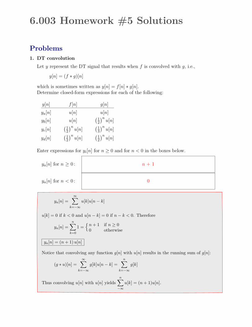
y[n] f [n] g[n] ya[n] u[n] u[n] n 1

2yb[n] u[n] u[n] n n12

13yc[n] u[n] u[n] n n1

212yd[n] u[n] u[n]

Enter expressions for yi[n] for n ≥ 0 and for n < 0 in the boxes below.

ya[n] for n ≥ 0 :

ya[n] for n < 0 :

n + 1

0

ya[n] = ∞n

k=−∞

u[k]u[n − k]

u[k] = 0 if k < 0 and u[n − k] = 0 if n − k < 0. Therefore

ya[n] = nn

k=0

1 =

n + 1 if n ≥ 0 0 otherwise

ya[n] = (n + 1) u[n]

Notice that convolving any function g[n] with u[n] results in the running sum of g[n]:

(g ∗ u)[n] = ∞n

k=−∞

g[k]u[n − k] = nn

k=−∞

g[k]

Thus convolving u[n] with u[n] yields nn

−∞ u[k] = (n + 1)u[n].

- -

2 6.003 Homework #5 Solutions / Fall 2011

yb[n] for n ≥ 0 : 2 − -

1 2

n

yb[n] for n < 0 : 0

n+1

1 2

yc[n] for n ≥ 0 :

yc[n] for n < 0 :

n n1 13 − 22 3

0

yd[n] for n ≥ 0 :

yd[n] for n < 0 :

- (n + 1) 1

2

n

0

yd[n] = ∞n

k=−∞

-1 2

k u[k]

-1 2

n−k u[n − k] =

-1 2

n nn

k=0

(1)k = (n + 1) -

1 2

n

yd[n] = (n + 1) -

1 2

n u[n]

Notice that this is the same as the unit-sample response of a system with a double pole at z = 1

2 (and a double zero at z = 0).

yb[n] =∞∑

k=−∞u[k]

(12

)n−ku[n− k] =

n∑k=0

(12

)n−k=

0∑m=n

(12

)m=

1−(1

2)n+1

1− 12

yb[n] =(

2−(

12

)n)u[n]

Notice that this is equivalent to the running sum of(

12

)nu[n].

yc[n] =∞∑

k=−∞

(13

)ku[k]

(12

)n−ku[n− k] =

(12

)n n∑k=0

(23

)k=(

12

)n 1−(2

3)n+1

1− 23

yc[n] =(

3(

12

)n− 2

(13

)n)u[n]

Notice that this is the same as the unit-sample response of a system with poles at z = 12

and z = 13 (and a double zero at z = 0).

3 6.003 Homework #5 Solutions / Fall 2011 2. CT convolution

Let y represent the CT signal that results when f is convolved with g, i.e.,

y(t) = (f ∗ g)(t)

which is sometimes written as y(t) = f(t) ∗ g(t). Determine closed-form expressions for each of the following:

y(t) f(t) g(t) ya(t) u(t) u(t) yb(t) u(t) e−tu(t) yc(t) e−tu(t) e−2tu(t) yd(t) e−tu(t) e−tu(t)

Enter expressions for the non-zero parts of yi(t) and the range of t for which the expression apply in the boxes below.

ya(t) for t ≥ 0 :

ya(t) for t < 0 :

t

0

ya(t) = ∞

−∞ u(τ )u(t − τ)dτ =

t

0 dτ = tu(t)

ya(t) = tu(t)

Notice that the convolution of any function g(t) with u(t) is equal to the indefinite integral of g(t):

(g ∗ u)(t) = ∞

−∞ g(τ)u(t − τ)dτ =

t

−∞ g(τ )dτ

Thus (u ∗ u)(t) = tu(t).

yb(t) for t ≥ 0 : 1 − e−t

yb(t) for t < 0 :

yb(t) = ∞

−∞ u(τ)e −(t−τ)u(t − τ)dτ = e −t

t

0 e τ dτ = e −t(e t − 1) = (1 − e −t)u(t)

yb(t) = (1 − e −t)u(t)

Notice that this is the indefinite integral of e−tu(t).

0

4 6.003 Homework #5 Solutions / Fall 2011

−2tyc(t) for t ≥ 0 : e−t − e

yc(t) for t < 0 : 0

yd(t) for t ≥ 0 : te−t

yd(t) for t < 0 : 0

yc(t) =∫ ∞−∞

e−τu(τ)e−2(t−τ)u(t−τ)dτ = e−2t∫ t

0eτdτ = e−2t(et−1) =

(e−t − e−2t)u(t)

yc(t) =(e−t − e−2t)u(t)

Notice that this is equal to the impulse response of a system with poles at s = −1 ands = −2.

yd(t) =∫ ∞−∞

e−τu(τ)e−(t−τ)u(t− τ)dτ = e−t∫ t

0dτ = e−tt = te−tu(t)

yd(t) = te−tu(t)

Notice that this is equal to the impulse response of a system with a double pole at s = −1.

5 6.003 Homework #5 Solutions / Fall 2011 3. Convolutions

Consider the convolution of two of the following signals.

a(t)

t

1

12

1

b(t)

t

1

12

1

c(t)

t

1

12

1

Determine if each of the following signals can be constructed by convolving (a or b or c) with (a or b or c). If it can, indicate which signals should be convolved. If it cannot, put an X in both boxes. Notice that there are ten possible answers: (a ∗ a), (a ∗ b), (a ∗ c), (b ∗ a), (b ∗ b), (b ∗ c), (c ∗ a), (c ∗ b), (c ∗ c), or (X,X). Notice also that the answer may not be unique.

14

1 2t

∗ =a or b or c or X a or b or c or X

b b

Must be asymmetric with large output at early times and smaller output at later times.

14

1 2t

∗ =a or b or c or X a or b or c or X

ab

ba

The output is symmetric, which could happen if one of the inputs is a flipped-in-time version of the other input. There are only a few such options. One is c ∗ c — but that would result in a triangle-shaped output. Another symmetric option is a∗b (or equivalently b ∗ a), which fits with the first interval being concave up.

14

1 2t

∗ =a or b or c or X a or b or c or X

X X

The output is symmetric, which could happen if one of the inputs is a flipped-in-time version of the other input. There are only a few such options. One is c ∗ c — but that would result in a triangle-shaped output. Another symmetric option is a∗b (or equivalently b ∗ a) — but that would be concave up in first interval. None of the provided functions could result in this output.

14

1 2t

∗ =a or b or c or X a or b or c or X

a a

Must be asymmetric with small output at early times and larger output at later times.

14

1 2t

∗ =a or b or c or X a or b or c or X

ac

ca

interval, but shifted and flipped in time. Thus the answer is a ∗ c or c ∗ a.

14

1 2t

∗ =a or b or c or X a or b or c or X

X X

6 6.003 Homework #5 Solutions / Fall 2011

The first interval looks like the integral of a. The second interval looks like the first

The step discontinuity in this result could only result if one of the convolved functions contains an impulse.

7 6.003 Homework #5 Solutions / Fall 2011

Engineering Design Problems 4. The L operator

The R (right-shift) operator can be used to express functional forms for any block diagram that is composed of adders, gains, and delays. Since the delay operation is causal (i.e., its output does not depend on future values of its input) functionals that build on R can only represent causal systems. Define the L (left-shift) operator to represent “anticipators," which are the anti-causal counterparts to delay elements. If X is an input sequence, then Y = LX means that y[n] = x[n + 1] for all n. Let H1 represent the system described by the following functional:

Y 1 H1 = = .

X 1 − 3L a. Determine a difference equation for this system.

y[n] − 3y[n + 1] = x[n]

b. Find the unit-sample response of this system.

Assume that the system is anti-causal and starts “at rest” so that y[n] = 0 for n > 0. Then we can solve the difference equation iteratively:

y[n] = x[n] + 3y[n + 1]

y[0] = 1 y[−1] = 3 y[−2] = 9 y[−3] = 27 y[−4] = 81

. . . y[−n] = 3n

y[n] = 3−n u[−n]

c. Determine the pole(s) of this system.

The unit-sample response has the form zn 0 = 3−n. Thus the pole is at z0 = 1

3 .

d. If a system is represented as the ratio of polynomials in R, then the poles of the system are the roots of the denominator polynomial after R is replaced by 1 . Determine an zanalogous rule for systems represented by a ratio of polynomials in L.

Subsitute L → z in the system functional. Reduce to a ratio of polynomials in z. Then the poles are the roots of the denominator.

Consider a system that is described by the following unit-sample response:

h2[n] =(

12

)|n|for all n .

8 6.003 Homework #5 Solutions / Fall 2011 e. Determine a closed-form functional representation for the system described by h2[n].

f. Determine the poles of the system in part e.

Substitute R → 1 z and L → z in the system functional:

H2(z) = 1 − 1

4 RL (1 − 1

2 R)(1 − 1 2 L)

= 1 − 1

4 (1 − 1

2 1 z )(1 − 1

2 z) =

3 4 z

(z − 1 2 )(1 − 1

2 z)

The poles are the roots of the denominator: z = 1 2 and 2.

g. Do a series expansion of the system function in part e (it may be helpful to use partial fractions). Explain the relation between the series and the unit-sample response h2[n].

We can express the functional for h2[n] as a polynomial in R and L:

H2 = 1 + 12R+

(12R)2

+(

12R)3

+ · · ·+ 12L+

(12L)2

+(

12L)3

+ · · ·

We can close the form by recognizing two power series

H2 =∞∑n=0

(12R)n

+∞∑n=0

(12L)n−1 = 1

1− 12R

+ 11− 1

2L−1 =

1− 14RL

(1− 12R)(1− 1

2L)

Each term in the series expansion

H2 = 1 + 12R+

(12R)2

+(

12R)3

+ · · ·+ 12L+

(12L)2

+(

12L)3

+ · · ·

corresponds to one point in the unit-sample response.

9 6.003 Homework #5 Solutions / Fall 2011

5. Upsampling

One way to enlarge an image is to upsample by linear interpolation, as follows.

a. Consider a one-dimensional signal x[n] whose non-zero samples are indexed from 0 to N (shown here for N = 3).

x[n]

n0 1 2 3 4 5

First, make a new signal w[n] defined by

w[n]

n0 1 2 3 4 5 6 7 8 9

Next, convolve w[n] with f [n] to produce y[n] = (w ∗ f)[n]. y[n] = (w ∗ f)[n]

n0 1 2 3 4 5 6 7 8 9

Determine f [n]. f [n]

n

1

b. Extend the linear interpolation method to two dimensions. Write a program that uses this method to enlarge the following image from its current dimensions (212 × 216) to three times those dimensions. Compare the result of linear interpolation with the result of replicating each pixel value 3 × 3 times (see appendix).

w[n] ={

x[n3 ] n = 0, 3, 6, . . . , 3N

0 otherwise .

10 6.003 Homework #5 Solutions / Fall 2011 The digital form of this image is available on the 6.003 website. The appendix contains sample Python code.

Program to enlarge image using bilinear interpolation.

import Image as im xx = im.open(’zebra.jpg’) # original image xpix = xx.load() aa = im.new(’L’,[xx.size[0]+2,xx.size[1]+2],0) # zero-pad edges aa.paste(xx,(1,1)) apix = aa.load() bb = im.new(’L’,[3*aa.size[0]-2,aa.size[1]],0) # horiz stretch bpix = bb.load() cc = im.new(’L’,[3*aa.size[0]-2,aa.size[1]],0) # horiz interpo­lated cpix = cc.load() dd = im.new(’L’,[3*aa.size[0]-2,3*aa.size[1]-2],0) # vertical stretch dpix = dd.load() yy = im.new(’L’,[3*aa.size[0]-2,3*aa.size[1]-2],0) # final answer ypix = yy.load() for j in range(aa.size[1]):

for i in range(aa.size[0]): # stretch image horizontally bpix[3*i,j] = apix[i,j]

for i in range(2,bb.size[0]-2): # convolve with triangle cpix[i,j] = 0.333*bpix[i-2,j]+0.666*bpix[i-1,j]+bpix[i,j]

+0.666*bpix[i+1,j]+0.333*bpix[i+2,j] for i in range(cc.size[0]):

for j in range(cc.size[1]): # stretch image vertically dpix[i,3*j] = cpix[i,j]

for j in range(2,dd.size[1]-2): # convolve with triangle ypix[i,j] = 0.333*dpix[i,j-2]+0.666*dpix[i,j-1]+dpix[i,j]

+0.666*dpix[i,j+1]+0.333*dpix[i,j+2] yy.crop([3,3,yy.size[0]-3,yy.size[1]-3]).save(’zebraBilinear.jpg’)

11 6.003 Homework #5 Solutions / Fall 2011

Image produced by code provided in appendix.

12 6.003 Homework #5 Solutions / Fall 2011

Image produced by bilinear interpolation.

This image has fewer jaggy edges.

13 6.003 Homework #5 Solutions / Fall 2011 6. Smiley

n

Consider the sequence of 1’s and −1’s shown below as x[n].x[n]

n0

1

−1

In this x[n], there is a single occurrence of the pattern −1, −1, 1. It occurs starting at = 1 and ending at n = 3. One method to automatically locate particular patterns of

this type is called “matched filtering.” Let p[n] represent the pattern of interest flipped about n = 0. Then instances of the pattern can be found by finding the times when y[n] = (p ∗ x)[n] is maximized.

a. Determine a matched filter p[n] that will find occurrences of the sequence: −1, −1, 1. Design p[n] so that (p ∗ x)[n] has maxima at points that are centered on the desired pattern, i.e., at n = 2 for the sequence above.

The same approach can be used to find patterns in pictures by generalizing the convolu­tion operator to two dimensions:

∞ ∞n n y[n, m] = (x ∗ p)[n, m] = x[k, l]p[n − k, m − l] .

k=−∞ l=−∞

A file called findsmiley.jpg (which can be downloaded from the 6.003 website) contains

matched filtering will work best if matching white pixels AND matching black pixels contribute positively to the answer. For that reason, 255 and 0 may not be the optimum choices for the values associated with white and black pixels.

a random pattern of white pixels (coded as 255) and black pixels (0) as well as a single instance of the following smiley face:

b. Find the row and column of findsmiley that corresponds to smiley’s nose. Note:

6.003 Homework #5 Solutions / Fall 2011 14 Program to locate nose. I made an image file smiley.jpg to simplify the code. (By treating the desired target as a file, it was easy to debug the code with a different (simpler) image in a different file.) Notice that 127.5 is subtracted from each pixel value before applying the convolution operation. This results in the following possible outputs (per pixel):

image pixel smiley pixel result black black (−127.5) ∗ (−127.5) = +127.52

white white (127.5) ∗ (127.5) = +127.52

black white (−127.5) ∗ (127.5) = −127.52

white black (−127.5) ∗ (127.5) = −127.52

which were chosen so that both types of matches give the same output, both types of mismatches give the same output, and matches and mismatches give opposite signs. Also, 127.5 was added back to the result, so that the result of the convolution could be viewed as an image yy.

import Image as im

xx = im.open(’findsmiley.jpg’) xwidth,xheight = xx.size ww = im.open(’smiley.jpg’) wwidth,wheight = ww.size yy = im.new(’L’,[xwidth-wwidth+1,xheight-wheight+1]) ywidth,yheight = yy.size xpix = xx.load() wpix = ww.load() ypix = yy.load()

xmax = -10000 coords = [0,0] for j in range(xheight-wheight+1):

for i in range(xwidth-wwidth+1): ss = 0 for jj in range(wheight):

for ii in range(wwidth): ss += (xpix[i+ii,j+jj]-127.5)*(wpix[ii,jj]-127.5)/127.5+127.5

ypix[i,j] = ss/wwidth/wheight if ss>xmax:

xmax = ss coords = [i,j]

print coords[0]+3,coords[1]+3 yy.save(’answer.jpg’)

column = 765; row = 432.

c. One advantage of the matched filter method is that it works even when the signal contains some noise. One can make a noisy version of findsmiley using Python’s gauss function:

import random ... pix[i,j] += random.gauss(0,dev)

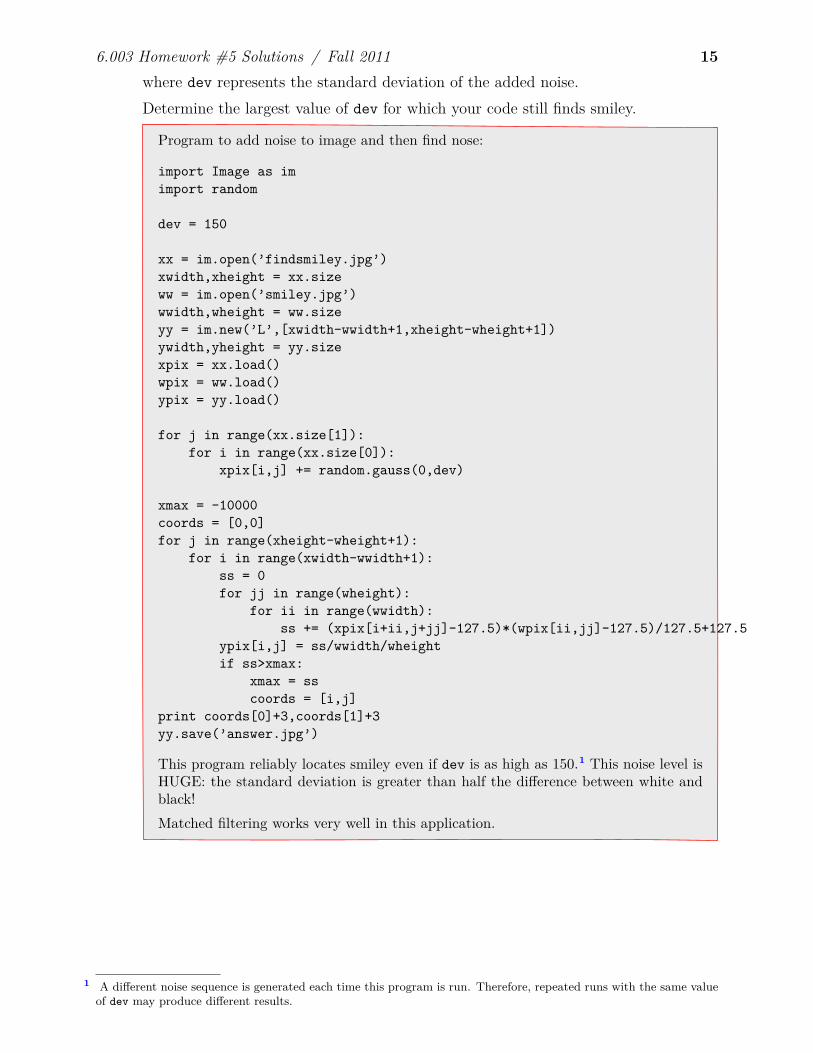
6.003 Homework #5 Solutions / Fall 2011 15 where dev represents the standard deviation of the added noise. Determine the largest value of dev for which your code still finds smiley.

Program to add noise to image and then find nose:

import Image as im import random

dev = 150

xx = im.open(’findsmiley.jpg’) xwidth,xheight = xx.size ww = im.open(’smiley.jpg’) wwidth,wheight = ww.size yy = im.new(’L’,[xwidth-wwidth+1,xheight-wheight+1]) ywidth,yheight = yy.size xpix = xx.load() wpix = ww.load() ypix = yy.load()

for j in range(xx.size[1]): for i in range(xx.size[0]):

xpix[i,j] += random.gauss(0,dev)

xmax = -10000 coords = [0,0] for j in range(xheight-wheight+1):

for i in range(xwidth-wwidth+1): ss = 0 for jj in range(wheight):

for ii in range(wwidth): ss += (xpix[i+ii,j+jj]-127.5)*(wpix[ii,jj]-127.5)/127.5+127.5

ypix[i,j] = ss/wwidth/wheight if ss>xmax:

xmax = ss coords = [i,j]

print coords[0]+3,coords[1]+3 yy.save(’answer.jpg’)

This program reliably locates smiley even if dev is as high as 150.1 This noise level is HUGE: the standard deviation is greater than half the difference between white and black! Matched filtering works very well in this application.

1 A different noise sequence is generated each time this program is run. Therefore, repeated runs with the same value of dev may produce different results.

MIT OpenCourseWarehttp://ocw.mit.edu

6.003 Signals and SystemsFall 2011 For information about citing these materials or our Terms of Use, visit: http://ocw.mit.edu/terms.