How Recent XRF Developments Impact Plant Based Alloy Material Testing

Kenneth L. SMITH

Olympus-Innov-X, 100 Sylvan Road, Suite 500, Woburn, MA 01890, USA; Phone: +011

781-569-1700; Fax +011 781-938-0128; Ken.Smith@OlympusNDT.com

Abstract

This article discusses advantages of non-destructive, on the spot alloy analysis. The utility of Hand-held XRF is

explained in practical terms that apply directly to industrial material testing. Beyond an overview of the

technology and its traditional uses, remarkable recent developments are identified and their impact is related

directly to alloy PMI. Dramatically improved hardware and software bring a new level speed, a wider elemental

range, and an improved accuracy to the field-testing of alloy materials. Specifically, 10x better detector

performance, 5 to 50 times better sensitivity for most elements, a new ability to analyze light elements such as

Mg, Al, Si, P, and S, high temperature “in-service” testing, and beam collimation for superior weld analysis are

among the innovations discussed.

Keywords: X-ray Fluorescence (XRF), Hand-held XRF (HH-XRF), Silicon Drift Detector (SDD), Ionization,

Positive Material Identification (PMI), Alloy Grade Identification

1 Introduction

For industrial component suppliers or industrial plant operations, alloy grade ID / material

verification is a key concern. Whether for corrosion resistance, temperature tolerance, or

mechanical characteristics, alloys are specified by design. An alloy material mix-up can result

in component failure. Component failure costs include down time, repair and replacement,

lost (leaking) material, environmental and fire hazards, or batch contamination.

HH-XRF is a fast, non-destructive way to confirm alloy grade. Whether producing

components, receiving alloy materials, installing pipes, valves, or other mission critical items,

or just a simple confirmation check of in-service process systems, HH-XRF provides rapid,

definitive material confirmation. HH-XRF users can quickly ID material mix-ups, improve

material control processes, and enjoy a rapid return on investment.

1.1 Basics of Hand-held XRF

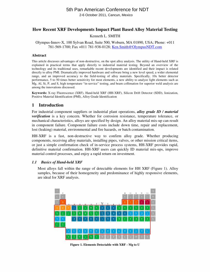
Most alloys fall within the range of detectable elements for HH XRF (Figure 1). Alloy

samples, because of their homogeneity and predominance of highly responsive elements,

are ideal for XRF analysis.

Figure 1. Elements Detectable with XRF - Mg to U

5th Pan American Conference for NDT 2-6 October 2011, Cancun, Mexico

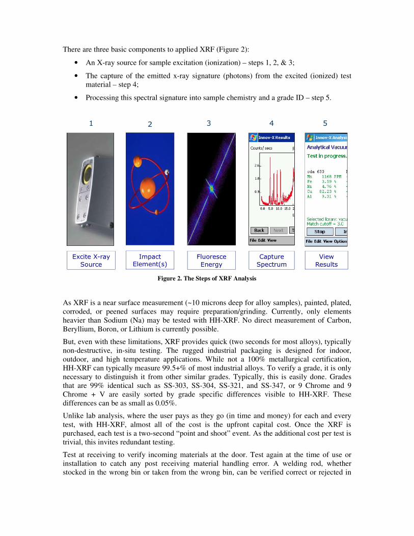
There are three basic components to applied XRF (Figure 2):

• An X-ray source for sample excitation (ionization) – steps 1, 2, & 3;

• The capture of the emitted x-ray signature (photons) from the excited (ionized) test

material – step 4;

• Processing this spectral signature into sample chemistry and a grade ID – step 5.

Figure 2. The Steps of XRF Analysis

As XRF is a near surface measurement (~10 microns deep for alloy samples), painted, plated,

corroded, or peened surfaces may require preparation/grinding. Currently, only elements

heavier than Sodium (Na) may be tested with HH-XRF. No direct measurement of Carbon,

Beryllium, Boron, or Lithium is currently possible.

But, even with these limitations, XRF provides quick (two seconds for most alloys), typically

non-destructive, in-situ testing. The rugged industrial packaging is designed for indoor,

outdoor, and high temperature applications. While not a 100% metallurgical certification,

HH-XRF can typically measure 99.5+% of most industrial alloys. To verify a grade, it is only

necessary to distinguish it from other similar grades. Typically, this is easily done. Grades

that are 99% identical such as SS-303, SS-304, SS-321, and SS-347, or 9 Chrome and 9

Chrome + V are easily sorted by grade specific differences visible to HH-XRF. These

differences can be as small as 0.05%.

Unlike lab analysis, where the user pays as they go (in time and money) for each and every

test, with HH-XRF, almost all of the cost is the upfront capital cost. Once the XRF is

purchased, each test is a two-second “point and shoot” event. As the additional cost per test is

trivial, this invites redundant testing.

Test at receiving to verify incoming materials at the door. Test again at the time of use or

installation to catch any post receiving material handling error. A welding rod, whether

stocked in the wrong bin or taken from the wrong bin, can be verified correct or rejected in

the matter of two seconds. And, test again either on the installed component in-service or at

final QC before shipping.

A single test at receiving won’t catch downstream errors in fabrication or installation. The

goal of material testing is not only to confirm that the material is correct, but also to correct

the errant processes that cause mix-ups. Redundant testing is the fastest and easiest way to

find and eliminate material mix-ups.

Starting in the 1980s, field portable XRF was best suited for testing stainless steels, chrome-

molybdenum steels, nickel alloys, and cobalt alloys. Low Alloy Steels, Copper and Titanium

Grades have been handled in a more limited manner because identification of many of these

grades requires or benefits from the ability to directly measure light elements such as

Aluminum, Silicon, Sulfur, and Phosphorous. Aluminum grades were tested only in a very

limited basis. The direct measurement of Magnesium, Aluminum, and Silicon at levels below

0.5% is essential to meaningful testing of Aluminum. Table 1 (below) places typical Limits of

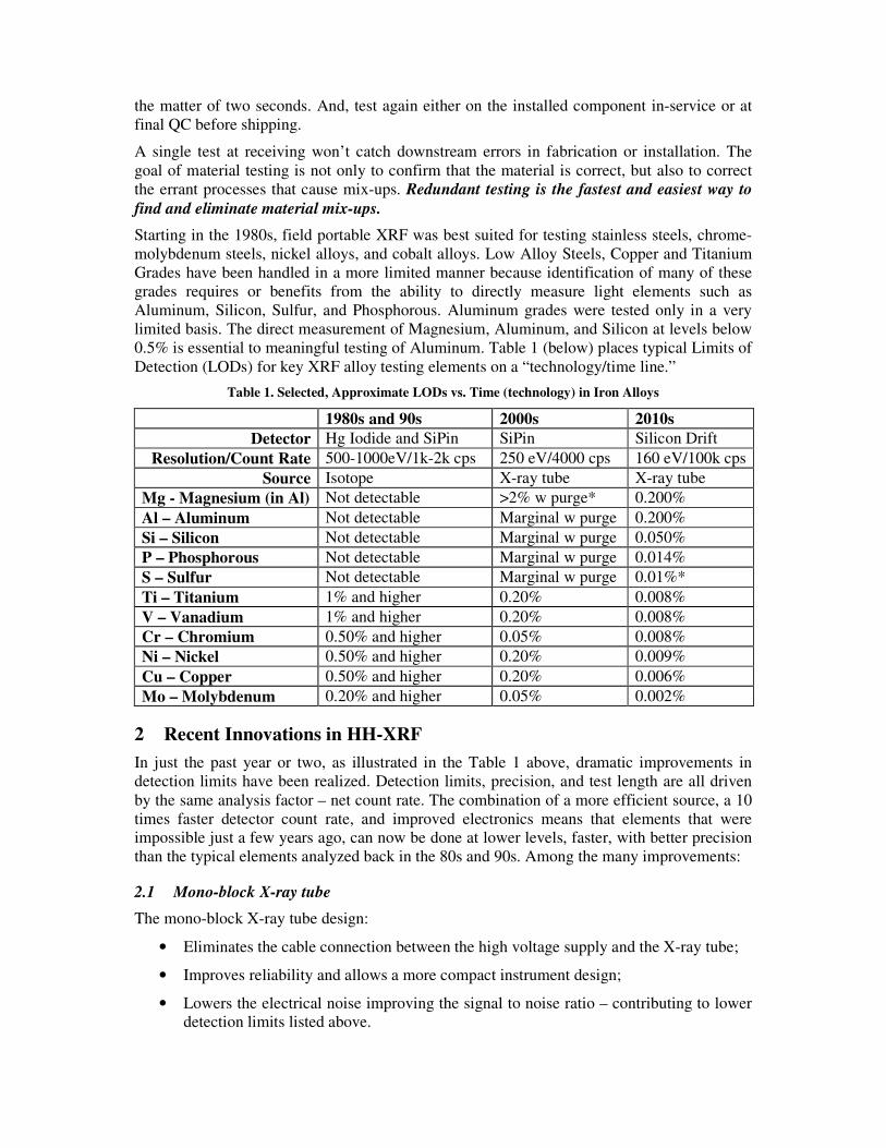
Detection (LODs) for key XRF alloy testing elements on a “technology/time line.”

Table 1. Selected, Approximate LODs vs. Time (technology) in Iron Alloys

1980s and 90s 2000s 2010s

Detector Hg Iodide and SiPin SiPin Silicon Drift

Resolution/Count Rate 500-1000eV/1k-2k cps 250 eV/4000 cps 160 eV/100k cps

Source Isotope X-ray tube X-ray tube

Mg - Magnesium (in Al) Not detectable >2% w purge* 0.200%

Al – Aluminum Not detectable Marginal w purge 0.200%

Si – Silicon Not detectable Marginal w purge 0.050%

P – Phosphorous Not detectable Marginal w purge 0.014%

S – Sulfur Not detectable Marginal w purge 0.01%*

Ti – Titanium 1% and higher 0.20% 0.008%

V – Vanadium 1% and higher 0.20% 0.008%

Cr – Chromium 0.50% and higher 0.05% 0.008%

Ni – Nickel 0.50% and higher 0.20% 0.009%

Cu – Copper 0.50% and higher 0.20% 0.006%

Mo – Molybdenum 0.20% and higher 0.05% 0.002%

2 Recent Innovations in HH-XRF

In just the past year or two, as illustrated in the Table 1 above, dramatic improvements in

detection limits have been realized. Detection limits, precision, and test length are all driven

by the same analysis factor – net count rate. The combination of a more efficient source, a 10

times faster detector count rate, and improved electronics means that elements that were

impossible just a few years ago, can now be done at lower levels, faster, with better precision

than the typical elements analyzed back in the 80s and 90s. Among the many improvements:

2.1 Mono-block X-ray tube

The mono-block X-ray tube design:

• Eliminates the cable connection between the high voltage supply and the X-ray tube;

• Improves reliability and allows a more compact instrument design;

• Lowers the electrical noise improving the signal to noise ratio – contributing to lower

detection limits listed above.

2.2 Advanced Grade Library Features and Functions

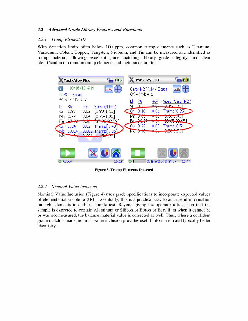
2.2.1 Tramp Element ID

With detection limits often below 100 ppm, common tramp elements such as Titanium,

Vanadium, Cobalt, Copper, Tungsten, Niobium, and Tin can be measured and identified as

tramp material, allowing excellent grade matching, library grade integrity, and clear

identification of common tramp elements and their concentrations.

2.2.2 Nominal Value Inclusion

Nominal Value Inclusion (Figure 4) uses grade specifications to incorporate expected values

of elements not visible to XRF. Essentially, this is a practical way to add useful information

on light elements to a short, simple test. Beyond giving the operator a heads up that the

sample is expected to contain Aluminum or Silicon or Boron or Beryllium when it cannot be

or was not measured, the balance material value is corrected as well. Thus, where a confident

grade match is made, nominal value inclusion provides useful information and typically better

chemistry.

Figure 3. Tramp Elements Detected

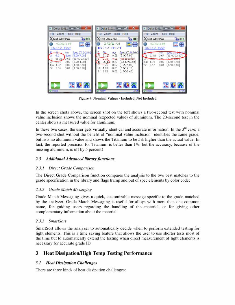
Figure 4. Nominal Values - Included, Not Included

In the screen shots above, the screen shot on the left shows a two-second test with nominal

value inclusion shows the nominal (expected value) of aluminum. The 20-second test in the

center shows a measured value for aluminum.

In these two cases, the user gets virtually identical and accurate information. In the 3rd

case, a

two-second shot without the benefit of “nominal value inclusion” identifies the same grade,

but lists no aluminum value and shows the Titanium to be 5% higher than the actual value. In

fact, the reported precision for Titanium is better than 1%, but the accuracy, because of the

missing aluminum, is off by 5 percent!

2.3 Additional Advanced library functions

2.3.1 Direct Grade Comparison

The Direct Grade Comparison function compares the analysis to the two best matches to the

grade specification in the library and flags tramp and out of spec elements by color code;

2.3.2 Grade Match Messaging

Grade Match Messaging gives a quick, customizable message specific to the grade matched

by the analyzer. Grade Match Messaging is useful for alloys with more than one common

name, for guiding users regarding the handling of the material, or for giving other

complementary information about the material.

2.3.3 SmartSort

SmartSort allows the analyzer to automatically decide when to perform extended testing for

light elements. This is a time saving feature that allows the user to use shorter tests most of

the time but to automatically extend the testing when direct measurement of light elements is

necessary for accurate grade ID.

3 Heat Dissipation/High Temp Testing Performance

3.1 Heat Dissipation Challenges

There are three kinds of heat dissipation challenges:

1. Testing in high ambient temperatures;

2. Testing of heated, in-service components;

3. Heavy-duty testing cycles (running many tests and long tests–60 seconds or more–

with only a few seconds between each test).

These challenges can occur separately or in combination.

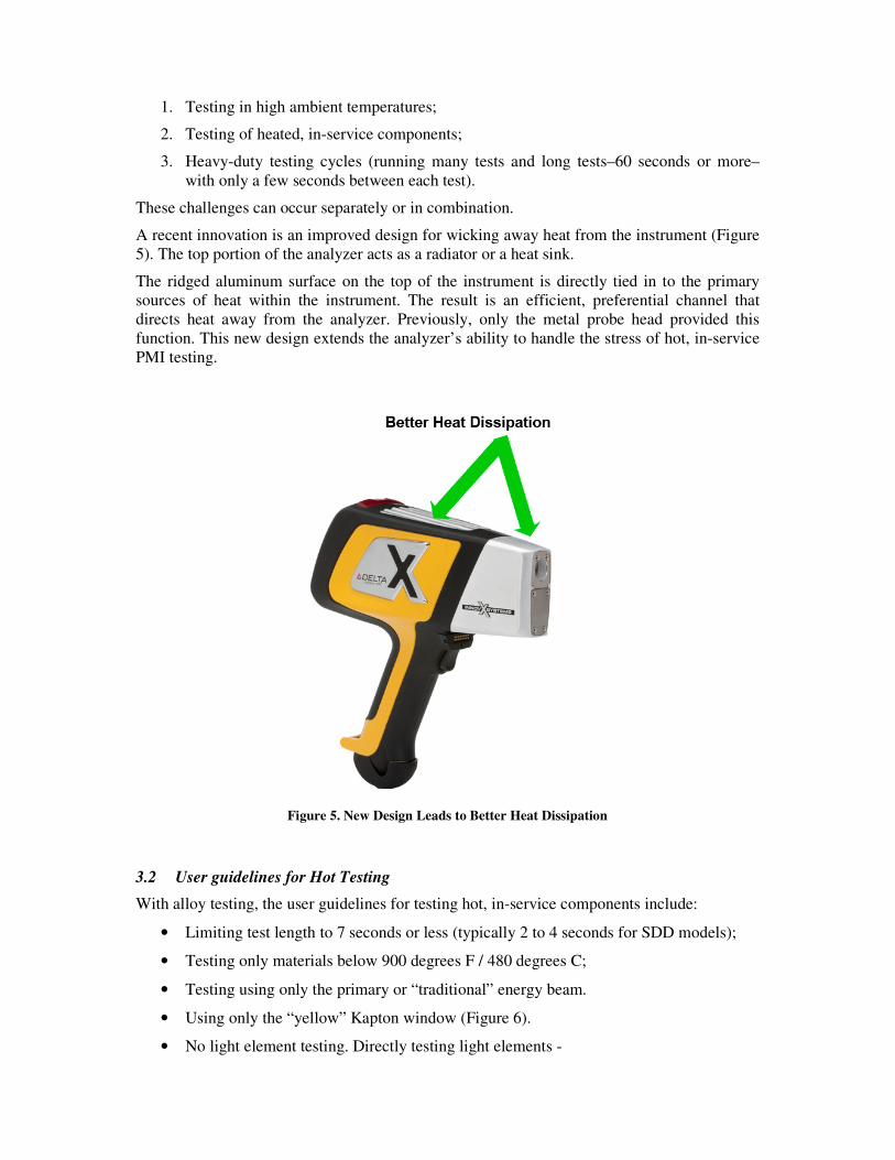
A recent innovation is an improved design for wicking away heat from the instrument (Figure

5). The top portion of the analyzer acts as a radiator or a heat sink.

The ridged aluminum surface on the top of the instrument is directly tied in to the primary

sources of heat within the instrument. The result is an efficient, preferential channel that

directs heat away from the analyzer. Previously, only the metal probe head provided this

function. This new design extends the analyzer’s ability to handle the stress of hot, in-service

PMI testing.

Figure 5. New Design Leads to Better Heat Dissipation

3.2 User guidelines for Hot Testing

With alloy testing, the user guidelines for testing hot, in-service components include:

• Limiting test length to 7 seconds or less (typically 2 to 4 seconds for SDD models);

• Testing only materials below 900 degrees F / 480 degrees C;

• Testing using only the primary or “traditional” energy beam.

• Using only the “yellow” Kapton window (Figure 6).

• No light element testing. Directly testing light elements -

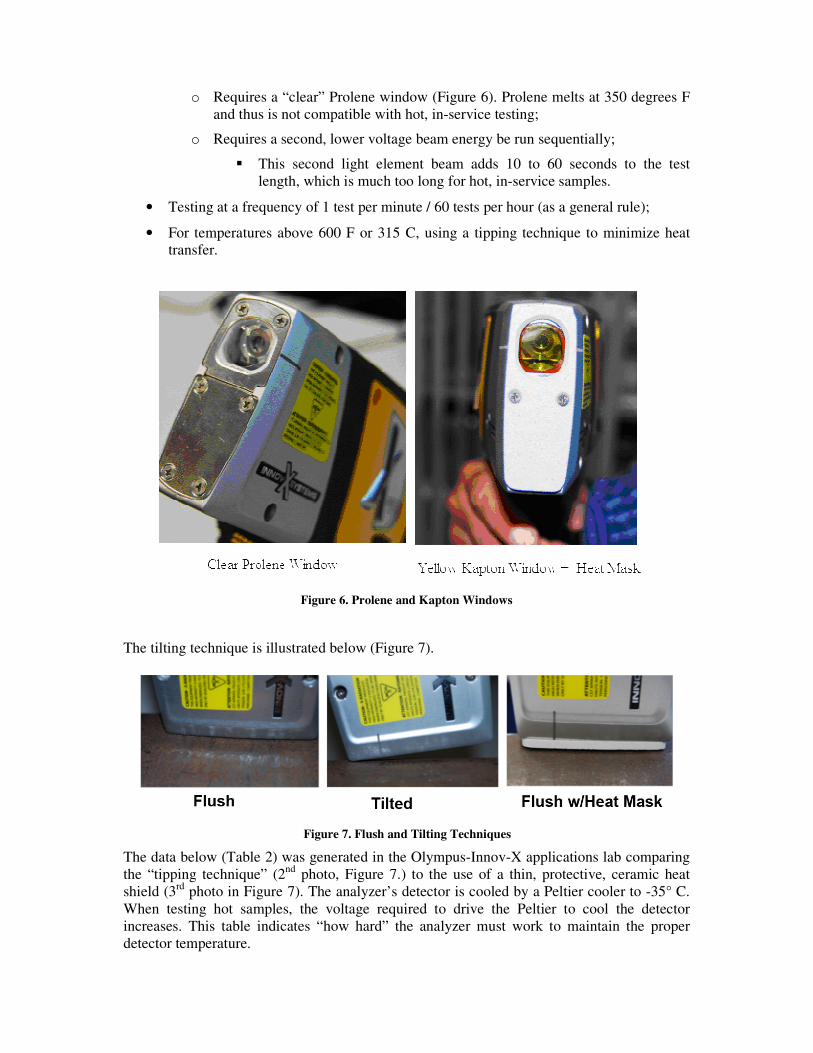
o Requires a “clear” Prolene window (Figure 6). Prolene melts at 350 degrees F

and thus is not compatible with hot, in-service testing;

o Requires a second, lower voltage beam energy be run sequentially;

� This second light element beam adds 10 to 60 seconds to the test

length, which is much too long for hot, in-service samples.

• Testing at a frequency of 1 test per minute / 60 tests per hour (as a general rule);

• For temperatures above 600 F or 315 C, using a tipping technique to minimize heat

transfer.

Figure 6. Prolene and Kapton Windows

The tilting technique is illustrated below (Figure 7).

The data below (Table 2) was generated in the Olympus-Innov-X applications lab comparing

the “tipping technique” (2nd

photo, Figure 7.) to the use of a thin, protective, ceramic heat

shield (3rd

photo in Figure 7). The analyzer’s detector is cooled by a Peltier cooler to -35° C.

When testing hot samples, the voltage required to drive the Peltier to cool the detector

increases. This table indicates “how hard” the analyzer must work to maintain the proper

detector temperature.

Figure 7. Flush and Tilting Techniques

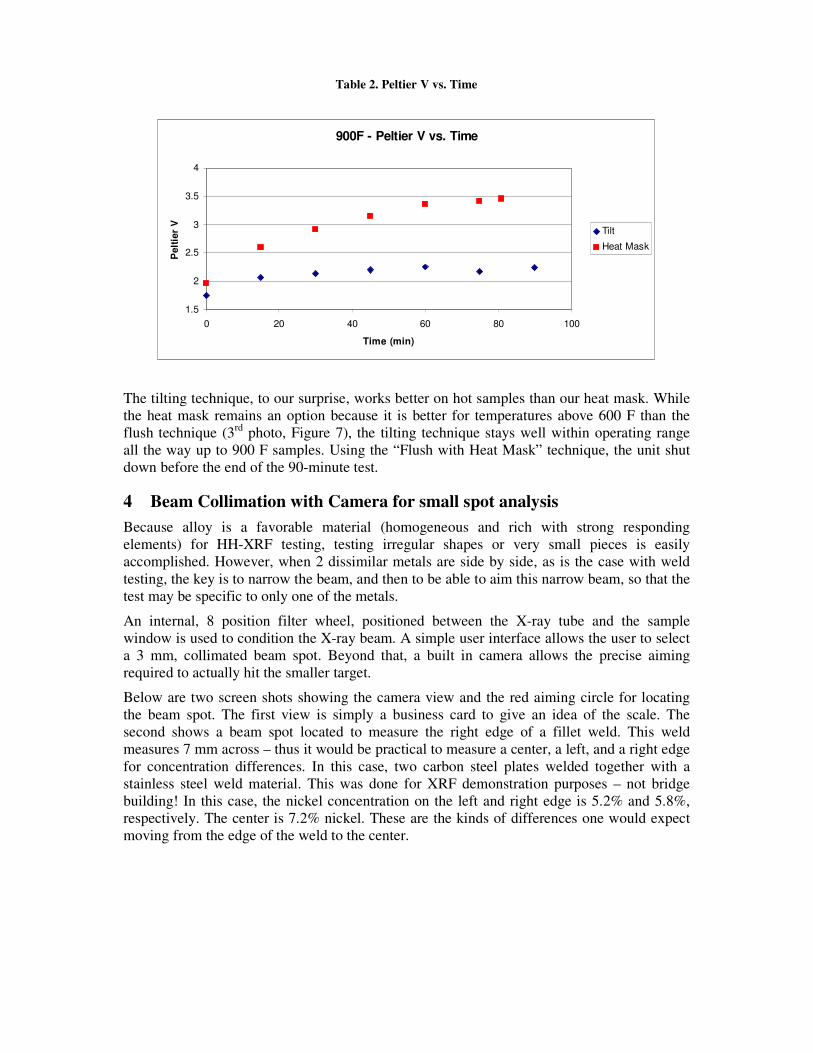
The tilting technique, to our surprise, works better on hot samples than our heat mask. While

the heat mask remains an option because it is better for temperatures above 600 F than the

flush technique (3rd

photo, Figure 7), the tilting technique stays well within operating range

all the way up to 900 F samples. Using the “Flush with Heat Mask” technique, the unit shut

down before the end of the 90-minute test.

4 Beam Collimation with Camera for small spot analysis

Because alloy is a favorable material (homogeneous and rich with strong responding

elements) for HH-XRF testing, testing irregular shapes or very small pieces is easily

accomplished. However, when 2 dissimilar metals are side by side, as is the case with weld

testing, the key is to narrow the beam, and then to be able to aim this narrow beam, so that the

test may be specific to only one of the metals.

An internal, 8 position filter wheel, positioned between the X-ray tube and the sample

window is used to condition the X-ray beam. A simple user interface allows the user to select

a 3 mm, collimated beam spot. Beyond that, a built in camera allows the precise aiming

required to actually hit the smaller target.

Below are two screen shots showing the camera view and the red aiming circle for locating

the beam spot. The first view is simply a business card to give an idea of the scale. The

second shows a beam spot located to measure the right edge of a fillet weld. This weld

measures 7 mm across – thus it would be practical to measure a center, a left, and a right edge

for concentration differences. In this case, two carbon steel plates welded together with a

stainless steel weld material. This was done for XRF demonstration purposes – not bridge

building! In this case, the nickel concentration on the left and right edge is 5.2% and 5.8%,

respectively. The center is 7.2% nickel. These are the kinds of differences one would expect

moving from the edge of the weld to the center.

900F - Peltier V vs. Time

1.5

2

2.5

3

3.5

4

0 20 40 60 80 100

Time (min)

Pelt

ier

V

Tilt

Heat Mask

Table 2. Peltier V vs. Time

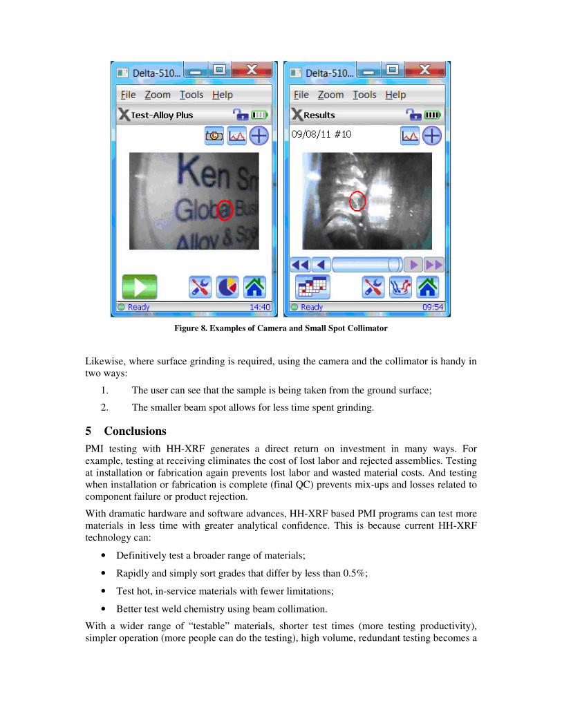
Figure 8. Examples of Camera and Small Spot Collimator

Likewise, where surface grinding is required, using the camera and the collimator is handy in

two ways:

1. The user can see that the sample is being taken from the ground surface;

2. The smaller beam spot allows for less time spent grinding.

5 Conclusions

PMI testing with HH-XRF generates a direct return on investment in many ways. For

example, testing at receiving eliminates the cost of lost labor and rejected assemblies. Testing

at installation or fabrication again prevents lost labor and wasted material costs. And testing

when installation or fabrication is complete (final QC) prevents mix-ups and losses related to

component failure or product rejection.

With dramatic hardware and software advances, HH-XRF based PMI programs can test more

materials in less time with greater analytical confidence. This is because current HH-XRF

technology can:

• Definitively test a broader range of materials;

• Rapidly and simply sort grades that differ by less than 0.5%;

• Test hot, in-service materials with fewer limitations;

• Better test weld chemistry using beam collimation.

With a wider range of “testable” materials, shorter test times (more testing productivity),

simpler operation (more people can do the testing), high volume, redundant testing becomes a

more cost effective strategy. More material mix-ups can be prevented and corrected at a far

lower cost per test.

In the end, whether it is process up-time or customer satisfaction, no organization wants to be

part of a material mix-up. Rapid, redundant HH-XRF testing provides a practical, cost

effective solution.