Embed Size (px)
Citation preview

5. Quantitative determination of additives by NMR


Determination of additives. NMR
97
5.1. Introduction
Nuclear Magnetic Resonance (NMR) is a versatile technique since it offers a
high number of signals of different molecules in a single spectrum. No other
spectroscopic method contains equally detailed structural and dynamic information
about chemical systems under investigation.1 The availability of high field instruments
in conjunction with improvements in probe design and electronic performance have
considerably increased sensitivity, resolution, precision and applicability of quantitative
NMR (qNMR) determinations from the beginning of the nineties.2 Quantitative NMR
has gained growing interest among the analytical chemists ever since and it has been
successfully applied in numerous fields.
In general, in classical analytics, the determination of a concentration usually
requires a specific method and a reference standard. In most of papers dealing with
qNMR, the quantification process is made on the basis of the choice of an adequate
signal for every analyte of interest and its integration with regard to the chosen internal
standard. The choice of the integrated signal both for the analyte and for the internal
standard are critical in order to develop a method with wide application and good
precision. A wrong decision can strongly affect the result, especially in the case of
crowded spectra with impurity signals overlapping resonance. Thus, it has been usually
advised, whenever possible, to take isolated and sharp peaks for the analytes. The
internal standard, on the other hand, must be soluble in the solvent of choice, stable
under working conditions, not reactive with any of the analytes and it should have an
intense singlet in a free region of the NMR spectrum.2 This is probably the main
limitation of qNMR, as far as there is a need of human intervention during processing
operations that closely influence integral values. Nevertheless, although several
software commands are available in order to reduce at minimum the subjective
decisions of the operator, they have demonstrated to perform worse than manual
processing made by a skilled operator.3
In the last few years, however, the increasing apparition of powerful computers
and softwares has led to the increase of the number of applications of chemometrics to
NMR signals, as far as a huge amount of data is produced and sometimes peaks for

Determination of additives. NMR
98
analytes are strongly overlapped.1
Thus, several references applying
chemometric tools in the NMR spectra of oils,4 tobaccos,
5 alcohols mixtures
1 biological
samples6 can be found and a paper comparing the results obtained in quantification by
PLS and by integration of signals in the spectra is also available.3 In general, PLS
clearly improves the accuracy of the quantifications and furthermore, it allows the
determination of components with partially overlapped signals in the spectrum. A
reference dealing with CLS for NMR spectra is reported as well.7 When the number of
calibration samples is reduced, this technique proves to outperform PLS.
Although no previous papers dealing with NMR in electroplating have been
found, the organic composition of the additives converts NMR to a suitable technique
so that additives can be quantified. The problem arises from the fact that plating baths
contain a great amount of inorganic salts; in the case of a nickel bath this means a huge
concentration of nickel paramagnetic ions. The existence of unpaired electrons in a
molecule modifies the magnetic field observed by the resonating nuclei and the
chemical shifts as well as the relaxation times are affected. This demands the search of a
method to eliminate the nickel ions from the solution prior to NMR spectrum
acquisition.
In the present study, a method for nickel elimination is reported, so that
reproducible NMR spectra for the additives can be obtained. The four additives of the
nickel bath (A-5(2X), SPB, SA-1 and NPA) provide NMR signals. Univariate
calibration procedures as well as PLS and CLS multivariate methods are applied and
compared, and UV-Vis spectrophotometry is applied as a reference technique for A-
5(2X) and SPB additives.

Determination of additives. NMR
99
5.2. Experimental
5.2.1. Reagents
A volume of 1.8 L of a commercial nickel bath (Supreme Plus brilliant, Atotech
formulation) was used with the following composition: NiSO4·6H2O (250 g L-1),
NiCl2·6H2O (50 g L-1) and H3BO3 (45 g L
-1) as non-additive solution; and SA-1 (2.6 ml
L-1), A-5(2X) (20 ml L
-1), NPA (2 ml L
-1) and Supreme Plus Brightner (SPB) (1 ml L
-1)
as additives (additives from Atotech, Berlin, Germany). The chemical composition of
additive solution is unkown. The final pH was 4 and it was maintained constant along
the process with addition of either NiCO3 or H2SO4 as required. Non-additive chemicals
were of analytical reagent grade (Panreac or Fluka) and used without further
purification. Additives were obtained from Atotech (Berlin, Germany) and used as
received. Doulby distilled water was used throughout. An amount of 0.00150 g of 3-
(trimethylsilyl)-2,2,3,3-tetradeuteroprionic acid sodium salt (TSP) dissolved in 5 mL of
D2O was used as a reference for δ = 0.00 ppm. An amount of 10 mL of succinic acid
(20g/L) was also prepared. Succinic acid is used as a calibration standard in NMR.
NaOH 10 M was used to precipitate Ni2+ ions from the nickel bath. Hydrochloric acid at
several dilutions, from concentrated (37%) to diluted (0.5M), were also used to adjust
the pH value of the supernatant, after Ni2+ precipitation, between 3.95 and 4.05 before
the NMR measurement.
5.2.2. Apparatus
A vessel with a water jacket (Afora, Barcelona, Spain) for the nickel bath
(65ºC), a Crison 501 pH meter (Alella, Spain); a Haake water bath thermostat controlled
by an external probe dipped into the nickel bath and a rectifier (±20A/30V) from HQ
Power (Nedis BV, The Netherlands) (model no. PS 3020) were used for
electrodeposition. A Bruker Avance-500 spectrophotometer was used to record 500
mHz 1H-NMR spectra at a temperature of 30ºC. An amount of 128 scans of 64 K data
points was acquired every time with a spectral width of 8012 Hz (16 ppm), acquisition
time of 2.2 s., recycle delay of 9.0 s., flip angle of 90 º and a constant gain of 11585.
The solvent signal suppression was achieved using the watergate pulse sequence.8 The
data were acquired under an automatic procedure, requiring about 24 min per sample.

Determination of additives. NMR
100
Micropipettes Brand (Wertheim, Germany) or Eppendorf (Hamburg, Germany) were
used throughout.
5.2.3. Software and data processing
Preliminary data processing was carried out with Bruker software, TOPSPIN
1.3. The Free induction Decay (FID) signals were Fourier transformed (1.0 Hz line
broadening) and the spectra were phased and the baseline corrected. The resulting
spectra were aligned by right or left shifting as necessary, using the TSP signal as a
reference. Data analysis was achieved with MestRe-C 4.8.6.0 software package
(Santiago de Compostela University, Spain). The Unscrambler v. 9.7 (Camo A/S,
Trondheim, Norway, 2007) software package, which allowed the application of PLS,
was used. Matlab 7.4.0 software (The Mathworks Inc., Natick, USA) was used for CLS
and icoshift algorithm was also used for peaks alignment.
To test the prediction capability of the developed models by PLS, the statistic
relative error (RE, see introduction) was used. The calibration and prediction
(validation) sets were defined before any data processing and remained unchanged
along the work. The leave-one-out full Cross-Validation procedure was used to assess
the robustness of the constructed models. Choosing the optimum number of factors
(LVs) to be used with the PLS model was made through the method explained in
section 1.2.3. of the Introduction.
5.2.4. Procedures
5.2.4.1. Sample preparation and NMR spectra acquisition
A volume of 19.25 µL of acid succinic solution was added to 2.5 mL of the
nickel bath solution to be analysed. Succinic acid was used as inner standard for the
NMR signals. Then, 3.5 mL of NaOH 10 M were added in order to remove Ni(II) from
the solution through the formation of nickel hydroxide precipitate. The process was
assisted by proper agitation with a glass stick and a combination of heating and
agitation in an ultrasound during 5 min at 65ºC. After cooling, the solution was
centrifuged during 5 min at 4000 rpm. Then 1.0 mL of HCl (37%) was added onto a

Determination of additives. NMR
101
volume of 2.5 ml of the supernatant solution and the pH was adjusted approximately to
4.0 (a pH range between 3.95 and 4.05 was considered acceptable) with diluted
solutions of HCl. Afterwards, the solution was taken to 10 mL with HCl 10-4M (pH=
4.00). A volume of 500 µL of this final solution was placed in a 5 mm NMR tube and
50 µL of the D2O-TSP solution were added. D2O served as the field frequency lock. The
final concentrations were TSP 4.1·10-3 g L
-1 and D2O 11%. The whole process entails a
dilution of 10.6 fold from the original bath concentration. A sketch of the process is
depicted in Figure 1.
Figure 1. Sketch of the process for sample preparation and NMR measurement.
Nickel sample + inner Standard (Succinic Acid)
NaOH + Q + Agitation
Ni precipitate (discard) Solution
(3.Trimethylsilyl) propionic-2,2,3,3-d4 acid sodium salt
(TSP,δ=0ppm) in D2O
NMR signal acquisition
500 MHz 1H-NMR spectra were recorded using a Bruker DRX-500
[Acquisition time(Aq)=2.2s, Delay (d1)=9s, nºscan (ns)=128]
Determination of additives. NMR
102
5.2.4.2. Calibration
Two binary and one cuaternary calibration matrices were built. The first matrix
(named “A”) consisted of 36 samples with concentrations of 5, 10, 15, 20 and 25 mL/L
for A-5(2X) and 0.1, 0.25, 0.50, 0.75, 1.0 and 1.25mL/L for SPB. The rest of bath
components were at their standard concentration in the nickel bath (Section 3.2.1.). The
second matrix (named “B”) consisted of 30 samples with concentrations of 0.1, 0.5, 1.3,
2.5 and 3 mL/L for SA-1 and 0.5, 1, 1.5, 2 and 2.5 mL/L for NPA. The rest of bath
components were at their standard concentration in the nickel bath (Section 3.2.1). The
cuaternary calibration matrix (named “C”) consisted of 25 samples, with concentrations
of 10, 15, 20 and 25 mL/L for A-5(2X), 0.1, 0.25, 0.75 and 1.25 mL/L for SPB, 0.5, 1.3,
2.5 and 3.0 mL for SA-1 and 1.0, 1.5, 2 and 2.5 mL/L for NPA (Figure 2). The amount
of samples and concentration ranges are summarised in Table 1.
Figure 2. Cuaternary matrix (C). Circles are calibration samples and squares are validation
samples. Doubled symbols are replicated samples. The concentration values in mL L-1 in the
bath are given in parenthesis in the order: (A-5(2X), SPB, SA-1, NPA).
(10,1.0.75,0.5,1.5)
(10,1.25,0.5,1)
(10,0.25,0.5,2)
(10,0.1,0.5,2.5)
(10,0.75,1.3,1)
(10,0.25,2.5,1)
(10,0.1,3,1)
(10,0.25,1.3,1.5)
(10,0.1,1.3,2)(10,0.1,2.5,1.5)
(15,0.75,0.5,1)
(15,0.25,1.3,1)(15,0.1,2.5,1)(15,0.25,0.5,1.5)
(15,0.1,1.3,1.5)
(20,0.25,0.5,1)(20,0.1,1.3,1)
(25,0.1,0.5,1)
(15,0.1,0.5,2)
(20,0.1,0.5,1.5)

Determination of additives. NMR
103
Table 1. Built matrices and range of concentrations. All samples contained 250gL-1
NiSO4·6H2O, 50mLL-1 NiCl2·6H2O and 45 gL
-1 H3BO3 as non-additive solution.
Replicates were always kept in the same set.
To make a study on accuracy and precision, nine bath samples at several fixed A-5(2X),
SPB, SA-1 and NPA levels were randomly measured seven times each.
Nickel electrodeposition
The procedure of electrodeposition is explained in detail in section 3.2.4.1.
5.2.4.3. Additive determination in an electrolytic bath
Volumes of 2.5 mL were regularly extracted from the bath during
electrodeposition until the nickel bath was considered to be run out. A total of 20
aliquots were measured along the whole process.
5.3. Results and discussion
5.3.1. NMR spectra
All the additives in a nickel bath show NMR signal (Figure 3). A-5(2X) (2) and
NPA (11) show signals where no other bath component absorbs. SPB and SA-1 show
independent signals, (1) and (3) respectively, but also they both show the ensembled
signals (4) and (6). Signal (5) is for water, signal (8) is for the internal standard, succinic
acid, and signal (12) is for the displacement reference, TSP (δ=0 ppm). New peaks
coming from the degradation of the additives arise as well as current passes through;
they correspond to signals (7), (9) and (10).
Calibration
matrix
Samples mL A-5(2X)/L
bath
mL SPB/L
bath
mL SA-1/L
bath
mL NPA/L
bath
A 36 5 - 25 0.1-1.25 2.6 2.0
B 30 20 1.0 0.1-3 0.5.-2.5
C 25 10-25 0.1-1.25 0.5-3 1.0-2-5
Determination of additives. NMR
104
-1012345678910
1
2a
2b 2c
2
3
4 6
8
9
12
5
7
10
11
1 3 11
Figure 3. NMR spectrum for a nickel bath sample at the standard conditions (in blue). Red
peaks are signals appearing along the electrodepostion process.
1. SPB; 2. A-5(2X); 3. SA-1; 4. SA-1 + SPB; 5. water; 6. SA-1 + SPB; 7. new peak 1.; 8.
inner standard, succinic acid; 9. new peak 2; 10. new peak 3; 11. NPA; 12. TSP (δ=0).
5.3.2. Quantitation of additives
Two different quantitation methodologies were followed: linear regression
quantitation using the ratio (additive area)/(internal standard area) as analytical signal
and multivariate calibration of unique regions for each analyte by PLS and CLS as
calibration algorithms applied to different X-data matrices.
In general, parameters chosen for building any regression model as well as the
results of the regression in samples used for calibration and validation are given. The
results reported in each case are those corresponding to the best regression model
obtained for each additive. The limit of detection (LOD) is also given as a figure of
merit in any case. Also, results for several replicates at fixed concentration levels are
obtained for each additive. Thus, accuracy and precision are determined for independent
samples, which can be considered as an external test set for the model. These samples
were prepared and measured several months after the measurement of the main part of
the calibration and validation samples was done.

Determination of additives. NMR
105
5.3.2.1. Univariate linear regression
A classical univariate calibration with NMR signals usually needs the use of an
internal standard. In the present case that need is even higher because the sample is
subject to the precipitation of nickel. The choice of succinic acid as internal standard for
quantitation was carefully accomplished taking into account that several assumptions
must be fulfilled. Thus, it was necessary to find a compound with a clear and simple
signal in the NMR spectra at pH 4 and not overlapping with any additive signal. It had
to be water-soluble and not excessively expensive because the internal standard must be
added from the beginning of the procedure. Bath aliquots were diluted 10.6 fold in the
NMR tubes after the whole pretreatment and this resulted in a high internal standard
consumption. The high price of TSP was the main reason for discarding it as internal
standard and after several tests carried out with several compounds, succinic acid finally
demonstrated to be a suitable and reliable internal standard.
The individual spectra were manually integrated for each analyte peak. Thus, in
each spectrum, the area of succinic acid was taken to 1.000 and the area of each additive
peak was calculated accordingly. The best models were obtained when the samples of
matrix A were used to quantify SPB and A-5(2X) and when the samples of matrix B
were used to quantify SA-1 and NPA additives. The calibration lines are shown in
Figure 4, where the validation sets are also represented. The calibration lines for A-
5(2X) (R2 = 0.989) and SA-1 (R
2 = 0.985) provide a better regression with lower errors
than those provided by SPB (R2 = 0.87) and NPA (R
2 = 0.80); so, lower errors should
be expected for the two first additives in prediction. The prediction samples (Figure 4)
confirm the expected results in every case. In table 2 some characteristics of the
calibration models together with the mean errors and the LOD value (3s criterion)9 in
each case is shown.
Determination of additives. NMR
106
Figure 4. Calibration lines for the nickel bath additives. Filled circles represent the calibration
data points; open circles indicate data points belonging to the validation set. (a), A-5(2X); (b),
SPB; (c), SA-1; (d), NPA. The analytical signal refers to the ratio analyte area / internal
standard area.
(a) (b)
(d) (c)
y = 0.2305x - 0.0605R2 = 0.9846
0
0.2
0.4
0.6
0.8
0 1 2 3
mL SA-1/L bath
rela
tive
area
y = 0.5435x - 0.0936R2 = 0.989
0
4
8
12
16
0 10 20 30
mL A-5(2X)/L bath
rela
tive
area
y = 0.2246x - 0.0091R2 = 0.8656
0
0.1
0.2
0.3
0 0.5 1 1.5
mL SPB/L bath
rela
tive
area
y = 0.1339x - 0.0171R2 = 0.7978
0
0.2
0.4
0.5 1.75 3
mL NPA/L bath
rela
tive
area

Determination of additives. NMR
107
Table 2.Concentration ranges, relative errors and LOD estimated,found in the
determination of the nickel bath additives using the linear calibration method.
The best prediction results are obtained for A-5(2X) and SA-1 as it could be
expected from the fact that the peak signals for both additives (Figure 3) are big enough
and, therefore, the peak area is easily calculated for quantification. This can be doubtful
in the case of peak number 3, when it is compared with peak number 1 and 11. Height is
similar in all three cases, but peak number 3 is much wider and the value of area
increases accordingly, and consequently the signal / noise ratio improves. The low
signals for SPB and NPA peaks, on the other hand, are responsible for the relatively
high mean errors found in both cases. The LOD values (Table 2) are a consequence of
the way in which they are calculated (LOD = 3m
s xy /) and so they depend on the
precision (s) and sensitivity (m) of the calibration line.
Independent studies on accuracy and precision are given in Table 3. They were
taken three months after the calibration models were built. The results obtained agree
with expectations obtained from Figure 4; that is, a good accuracy was always obtained,
but precision is good for A-5(2X) and for values high enough of SPB,
Additive Concentration
range (mL L-1
bath)
Set Number of
mixtures
Peak number
(Figure 3)
RE(%) LOD (mL L-1)
A-5(2X) 5-25 cala 23 2 4.9 2
valb 12 6.0
SPB 0.1-1.25 cala 15 1 11 0.3
valb 9 19
SA-1 0.1-3.0 cala 9 3 7.2 0.4
valb 9 11
NPA 0.5-2.5 cala 13 11 15 0.9
valb 9 13
acalibration samples
bvalidation samples

Determination of additives. NMR
108
Table 3. Accuracy and precision in the determination of additives in a nickel bath matrix by
NMR and linear calibration. Concentrations in mL additive/ L bath .Seven replicates.
Additive Taken
(mL L-1 bath)
Found
(mL L-1 bath)
Error
(%)
RSD
(%)
A-5(2X)a 5.0 5.4 7.8 13
5.0 4.8 -3.6 6.1
15.0 15.2 1.7 6.5
25.0 24.0 -3.9 2.7
25.0 24.4 -2.5 3.0
SPBb 1.25 1.17 -6.5 5.5
0.1e - - -
0.75 0.81 7.6 2.4
0.1e - - -
1.25 1.25 - -
SA-1c 1.3 1.2 -6.6 24
0.1e - - -
3.0 3.0 - -
3.0 3.2 6.7 16
NPAd 1.5 1.6 6.7 12
2.5 2.4 -5.8 2.0
0.5e - - -
2.5 2.1 -14 16
aThe A-5(2X) concentration ranged between 5.0 and 25 mL L-1. SA-1 and NPA were in the typical
values.
bThe SPB concentration ranged between 0.1 and 1.25 mL L-1. SA-1 and NPA were in the typical values.
cThe SA-1 concentration ranged between 0.1 and 3.0 mL L-1. A-5(2X) and SPB were in the typical
values.
dThe NPA concentration ranged between 0.5 and 2.5 mL L-1. A-5(2X) and SPB were in the typical
values.
eValues under the limit of detection that could not be determined.
Determination of additives. NMR
109
whereas it is only acceptable-poor in the case of SA-1 and NPA.
.
5.3.2.2. Multivariate calibration methods
Small pH changes as well as intermolecular interactions are responsible for peak
misalignments, what can lead to deteriorate the chemometric modelling 10,11
so, prior to
the multivariate modelling, all the acquired spectra were carefully aligned. The
alignment procedure was made with the icoshift (namely, interval co-rrelation shift-ing)
program, based on Correlation SHIFTing of spectral Intervals. The program has
demonstrated to be highly efficient in solving signal alignment problems in
metabonomic NMR data analysis and it works faster than similar methods found in the
literature.12
Unlike linear calibration, when multivariate methods are used no need of
normalization with an internal standard is required, because small errors in the amount
of sample taken can be modelled with some extra latent variables (LVs). Two kind of
calibration models were tried, namely CLS and PLS, but PLS always provided better
results than CLS, probably because the latter is more liable to signal variations,
interferences from the matrix, etc.
Table 4 summarizes the results obtained when PLS is applied. The part of the
NMR spectra used as data matrix in the PLS models depends on each analyte. Only
those variables with observable signal from a specific analyte were included, in order to
reduce the amount of noncorrelated variance in the data. It has been previously
demonstrated that models based on selected regions of the spectra have better predicting
ability and need a lower number of latent variables than if the whole NMR spectrum is
used.3 The limit the detection in the multivariate calibration was calculated through two
different methods: the Found vs. added plot13 and the Multivariate Residuals Value
(MR) 14, (see Section 1.2.6. of the Introducion).

Determination of additives. NMR
110
Table 4. Relative errors and LOD estimation found in the determination of bath additives using
PLS calibration method.
The number of LVs ranges between 1 and 3; the extra LVs above 1 are probably
due to the complexity of the matrix and to the absence of internal standard. Mean errors
for A-5(2X) and SA-1 are similar to those found with the univariate linear method, but
errors for SPB and NPA are lower than those found with the univariate linear method..
The final result is that PLS, as a whole, provides always a similar or lower mean errors
and more homogeneous; so the PLS model was chosen for calibration of additives.
Independent studies of accuracy and precision are given in Table 5. The were
run 1 month after the calibration models were built; this can probably explain why the
precision values are similar to those found when the model was built (Table 4), whereas
accuracy errors between 10 and 20% were found in a number of cases (Table 5). The
values of LOD are similar, regardless the calibration model or the method applied for
calculation, with the only exception of SA-1, where the LOD value ranges in a
magnitude order (Tables 2 and 4).
LOD (mL L-1) Additive Concentration
range mL L-1
bath
Set Number
of
mixtures
Peak
number
(Figure 3)
LVs RE
(%) Found vs.
added
MR
A-5(2X) 10-25 cala 15 2 3 4.1 2 4
valb 9 7.5
SPB 0.1-1.25 cala 8 1 1 7.5 0.3 0.7
valb 5 7.7
SA-1 0.5-2.5 cala 15 1+3+4+6 2 2.2 0.1 0.05
valb 8 4.5
NPA 1.0-2.5 cala 15 11 2 12 0.6 0.5
valb 10 9.0
acalibration samples
bvalidation samples

Determination of additives. NMR
111
Table 5. Accuracy and precision in the determination of additives in a nickel bath matrix by
NMR and PLS. Concentrations are in mL/L bath.
Additive Taken
(mL L-1 bath)
Found
(mL L-1 bath)
Error
(%)
RSD
(%)
A-5(2X)a 5.0 6.1 23 4.3
5.0 5.7 15 1.2
15.0 1.3.5 -9.8 8.4
25.0 23.2 -7.2 1.7
25.0 25.0 - 6.6
SPBb 1.25 1.12 10 4.3
0.1e - - -
0.75 0.70 -6.3 12
0.1e - - -
1.25 1.22 -2.3 11
SA-1c 1.3 1.1 -15 3.3
0.12 - - -
3.0 3.0 - 4.0
3.0 3.1 2.4 6.4
NPAd 1.5 1.5 - 8.2
2.5 2.1 -17 9.9
0.52 - - -
2.5 2.0 -20 5.4
aThe A-5(2X) concentration ranged between 5.0 and 25 mL L-1. SA-1 and NPA were in the typical
values.
bThe SPB concentration ranged between 0.1 and 1.25 mL L-1. SA-1 and NPA were in the typical values.
cThe SA-1 concentration ranged between 0.1 and 3.0 mL L-1. A-5(2X) and SPB were in the typical
values.
dThe NPA concentration ranged between 0.5 and 2.5 mL L-1. A-5(2X) and SPB were in the typical
values.
eValues under the limit of detection that could not be determined.

Determination of additives. NMR
112
5.3.3. Evaluation of the models
In general, the best results, as a whole, are obtained with PLS regression.
Electroplating baths are complex matrices with a number of compounds at very high
concentrations and, consequently, it was expected CLS to give poorer results than PLS.
However, PLS requires the preparation of a lot of calibration standards, what can
become an arduous task as long as samples require a previous procedure of nickel
elimination before NMR measuring. A similar problem happens with the univariate
method, but the number of standards, in general, is not so large and the technique does
not require any chemometric knowledge to build the models to quantify. Among the
drawbacks of linear regression, the need of an internal standard can be cited.
Sometimes, especially in the case of crowded NMR spectra, it can be an arduous task
the search of a standard whose resonance is not affected by the chemical composition of
the sample. Certainly, this is not the case, but even in these circumstances multivariate
techniques show as an interesting alternative to univariate methods.
5.3.4. Additive determination in a commercial electroplating nickel bath
The nickel bath preparation and the electrodeposition process have been
previously explained (Section 3.2.1. and 3.2.4.1.). The concentration of the four
additives in the bath can be monitored over time by taking periodically one aliquot and
measuring the NMR spectrum after proper pre-treatment are followed. The additives
concentration has been calculated using both linear calibration and PLS method.
Concentrations have been corrected to refer them to the initial bath volume. The reason
is that taking a volume of 2.5 mL of bath in each NMR aliquot represents a volume
reduction of 0.14% per aliquot and a final volume reduction of 2.8% at the end of the
electrodeposition. The results obtained for all the additives after using linear calibration
and PLS can be seen in Figure 5. Both methods (linear calibration and PLS) give similar
results, though the linear method tend to give slightly lower (and more imprecise)
values for A-5(2X) and SA-1. The additives A-5(2X) and NPA do not change much
their concentrations along the bath life, but SPB and SA-1 do it. Because of the high
LOD value, SPB can not be followed completely along the bath life, though this should
not be important if the main aim is to keep the additive concentration at its original
value.

Determination of additives. NMR
113
Figure 5. Evolution of the additives along the electroplating process. (a) A-5(2X); (b) SPB; (c)
SA-1 and (d) NPA. Filled circles, univariate calibration; filled squares, PLS. Open marks are
concentrations under the LOD when it is estimated by the found vs. added method.
Evolution of A-5(2X) and SPB additives followed by NMR (PLS calibration
method) has been compared to their evolution followed by UV-Vis spectrophotometry
(Figure 6). UV-Vis results were obtained and commented in the previous chapter 2.
UV-Vis spectrophotometry is, here, used as a reference technique.
(b)
(c) (d)
(a)
0
10
20
30
0 10 20 30
current (A·h/L)
mL
A5(
2X)/
L B
ath
0
0.25
0.5
0.75
1
0 10 20 30
current (A·h/L)
mL
SP
B/L
Bat
h
0
1
2
3
0 10 20 30
current (A·h/L)
mL
SA
-1/L
Bat
h
0
1
2
3
0 10 20 30current (A·h/L)
mL
NP
A/L
Bat
h

Determination of additives. NMR
114
Figure 6. (a) A-5(2X) and (b) SPB concentrations in the bath along electrodeposition process.
Circles, UV-Vis first derivative data (wavelengths from 256 to 296, PLS results). Squares, NMR
data (PLS results). Open marks correspond to concentrations that are theoretically beyond the
limit of detection of the analytical method calculated by the found vs. added method.
It can be concluded that NMR results are similar to UV-Vis results as far as accuracy is
considered, because both methods provide the same concentration. However, UV-Vis
data show a better precision and lower detection limit. Obviously, no comparison
between data beyond the LOD has been made. The LOD value of the NMR method
prevents its use to follow the SPB evolution during the last third of SPB concentration.
The additives SA-1 and NPA do not show any absorption in the UV-Vis region;
so that, the technique can not be used as a reference. Because of that, recovery studies
of both additives in spiked samples were made. Several bath aliquots were spiked with
known concentrations of the additives and the recovery concentration was then
calculated. This is made in order to check how the passage of both, time and current,
affects the bath matrix. Table 6 summarizes the results obtained when the PLS
regression method is applied.
(a) (b)
0
10
20
30
0 10 20 30
current (A·h/L)
mL
A-5
(2X
)/L
Bat
h
-0.05
0.30
0.65
1.00
0 10 20 30
current (A.h/L)
mL
SP
B/L
Bat
h

Determination of additives. NMR
115
Table 6. Concentrations of SA-1 and NPA additives found in nickel electroplating baths with
PLS calibration method applied to NMR data. Concentrations are in mL L-1.
Additive Found Added Total found Recovered Recovery(%)
SA-1 2.63 0.48 2.98 0.35 73
1.10 1.15 2.43 1.33 116
0.84 1.48 2.39 1.55 105
NPA 1.87 0.48 2.26 0.39 81
1.78 0.96 2.88 1.10 115
1.33 1.19 2.88 1.55 130
Recovery results stand between 73 and 130%, what could be expected considering the
random errors found in the estimation of both additives (Figures 4 and 5). However,
these results can be considered acceptable when data are obtained with bath control
purposes (see next chapter).
5.3.4.1. Degradation products
It was observed that some new peaks arise in the NMR spectrum as the nickel
bath is being used. (peaks 7, 9 and 10, Figure 1). Figure 7 shows such peaks for several
aliquots obtained along the bath life. The new compounds must, therefore, come from
the degradation of the original additives.
Figure 7. Degradation peaks evolution. ( aliquot 1; aliquot 5; aliquot 10;
aliquot 15; aliquot 20).
δ (ppm) δ (ppm) δ (ppm)

Determination of additives. NMR
116
0
1
2
0 10 20 30current (A·h/L)
rela
tive
area
2
1
3
Because the additive composition is unknown, so is the structure of their
degradation products, but the way in which the profile of the new peaks evolves can be
seen by plotting the peak area as a function of the current (Figure 8). The three peaks
show a similar evolution pattern. In this case, the experimental points in Figure 8 seem
to obey a pseudo-first-order growth law according to the equation:
)1( obsteareaarea κ−−= ∞ (1)
where:
area = integrated peak value at any time.
∞area = integrated peak at equilibrium.
Figure 8. Evolution of growing peaks along the nickel bath life. Correspondence with peaks in
Figure 3 : (1), peak No 7; (2), peak No 9; (3) peak No.10; Lines represent non-linear regression
analysis according to a pseudo-first-order growth, (Eq. (1)).
A first order law is a similar pattern to some plating bath precedents (see, for
instance, SPB decay in chapter 2 and reference 15). When non-linear least-square
regression analysis is applied according to Equation (1) to the experimental points, the
lines in Figure 8 are found. From the regression lines, the parameters ∞area and kobs
can be deduced and they are shown in Table 7.

Determination of additives. NMR
117
Table 7. Parameters values obtained from non-linear regression analysis applied to the data
points in Figure 8, according to Equation (1). Standard deviation is in parenthesis.
curve number ∞area kobs (A·h/L)
-1 r
1 1.2(0.1) 0.05(0.01) 0.98
2 1.4(0.1) 0.06(0.01) 0.98
3 2.8(0.3) 0.04(0.01) 0.99
The evolution of additives in the nickel bath is collected in Figure 9 (PLS
calibration) where some concentrations under LOD have been included (in the cases of
SA-1 and SPB) to show the tendence. The additives A-5(2X) and NPA do not
practically change their concentration along the process so they can not be a source of
degradation products. So degradation products should come either from SA-1 or from
SPB or, perhaps, from both of them. It has been shown in chapter 2 that SPB decays
according to a first-order law (kobs = 0.137±0.05 A·h/L). The SA-1 decay does not show
a definite pattern (Figure 9), but considering a pseudo-first order decay the rate law
would be:
[ ] [ ] tobseSASA
κ−−=− 011 (2)
or in the form shown in figure 9:
[ ]
[ ]t
obseSA
SA κ−=−−
01
1 (3)

Determination of additives. NMR
118
0
0.4
0.8
1.2
0 15 30
current (A·h/L)
[add
itive
]/[ad
ditiv
e]0
Figure 9. Evolution of additives in a nickel bath according to NMR data. All the data are
referred to the initial concentration of each additive to get comparable plots. Lines represent
non-linear regression analysis according to equation (3). Blue points, A-5(2X); green crosses,
NPA; Pink triangles, SA-1; red squares, SPB. Open marks are concentrations under LOD.
When non-linear regression analysis (equation 3) is applied to the experimental
points in Figure 9, value of kobs can be inferred at least with comparison purposes. The
data for regression analysis for both additives are in Table 8.
Table 8. Regression parameters obtained for SA-1 and SPB decays (equation 3). Standard
deviation in parenthesis.
Additive kobs (A·h/L)-1 r
SA-1 0.034(0.003) 0.94
SPB 0.113(0.013) 0.97
The values of kobs calculated for the three products growth (Table 7) are quite
similar to each other, so they might come from the same additive (the three peaks may
even correspond to the same species). Considering than the three products grow from
some additive decomposition/degradation, the growth and additive decay must have the
same rate constant. It is highly improbable that SPB is the source of the products
because its decay constant (0.11±0.01 (A·h/L)-1, table 8) is very different from the mean

Determination of additives. NMR
119
products growth constant (0.05±0.01 (A·h/L)-1. Nevertheless, SA-1 could be the source
of products (Figure 3, peaks number 7,9 and 10) because the SA-1 decay constant
(0.034±0.003 (A·h/L)-1) does not differ so much from the products growth constant
(0.05±0.01 (A·h/L)-1, Table 7). The supposition above agrees with the fact that both the
products growth and SA-1 decay do not seem to have reached the equilibrium at the end
of the bath life (Figures 8 and 9), whereas SPB decay has gone to completion at the end
of the bath life (Figures 6 and 9).
5.4. Conclusions
NMR has proven to be a suitable technique in order to follow the evolution of all
the additives in the bath provided that nickel ions are separated by precipitation with
NaOH. Univariate and multivariate methods can be applied and both methodologies
have demonstrated to give good results, but the best predictions are obtained when PLS
regression is applied. An important characteristic of multivariate techniques is the fact
that normalization vs. internal standard is not an essential task for quantification and
this is an important advantage for complex and crowded spectra.
Additives conversion into degradation products can be also appreciated as long
as peaks of additives decrease and new peaks arise along the electroplating process. The
study of the peaks evolution suggests that at least a new compound is formed, probably
from the degradation of SA-1.

Determination of additives. NMR
120
5.5. References
1 H. Winning, F. H. Larsen, R. Bro, S. B. Engelsen; J. Magn. Reson., 2008, 190, 26-32.
2 V. Rizzo, V. Pinciroli, J. of Pharm. Biom. Anal., 2005, 38, 851-857.
3 L. I. Nord, P. Vaag, J. Ø. Duus, Anal. Chem. 2004, 76, 4790-4798.
4 P. de Peinder, T. Visser, D.D. Petrauskas, F. Salvatori, F. Soulimani, B.M.
Weckhuysen, Vib. Spectroscop., 2009, 51, 205-212.
5 J. B. Wooten, N.E. Kalengamaliro, D.E. Alexon, Phytochemistry, 2009, 70, 940-951.
6 M. Dyrby, M. Petersen, A. K. Whitakker, L. Lambert, L. Nørgaard, R. Bro, S. B.
Engelsen, Anal. Chim. Acta, 2005, 531, 209-216.
7 O. V. Petrov, J. Hay, I. V. Mastikhin, B. J. Balcom, Food Res. Int., 2008, 41, 758-764.
8 M. Liu, X. Mao, C. Ye, H. Huang, J.K. Nicholson, J.C. Lindon., J. Magn. Reson.
1998, 132, 125-129.
9 L. A. Currie, Pure Appl. Chem., 1995, 67(10), 1699-1723.
10 I. Berregi, G. del Campo, R. Caracena, J. I. Miranda, Talanta, 2007, 72, 1049-1053.
11 T. Tynkkynen, M. Tiainen, P. Soininen, R. Laatikainen, Ana. Chim. Acta, 2009, 648,
105-112.
12 F. Savorani, G. Tomasi, S. B. Engelsen, J. Magn. Reson. 2010, 202(2), 190-202.
13 M.C. Ortiz, L. A. Sarabia, A. Herrero, M.S. Sánchez, M. B. Sanz, M.E. Rueda, D.
Gimenez, E, Meléndez, Chemom. Intell. Lab. Sys., 2003, 69, 21.
14 M. Ostra, C. Ubide, M. Vidal, J. Zuriarrain, Analyst, 2008, 133, 532-539.
15 A. Barriola, E. García, M. Ostra, C. Ubide, J. Electrochem. Soc., 2008, 155, D480-
D484.

6. Physical parameters for nickel plated sheets


Physical parameters for sheets
123
6.1. Introduction
During the last few years, the most of efforts in electroplating baths have been
focused on the study of chemical processes affecting electrodeposition. Nevertheless, the
quality assurance also involves the maintenance of the solution purity, the preparation of
surfaces to be coated or the use of proper techniques to ensure uniformity of the coatings.1
Numerous bath troubles have been approached through the visual observation of the plated
objects and through the measurement of physical properties. Studies on the stress, ductility,
tensile strength, hardness, leveling, roughness, morphology, dullness or adhesion effects of
nickel plated surfaces have frequently been accomplished with the aim of relating these
properties to the bath conditions such as pH, plating time, current density2,3
or additive
concentration.4,5
Also, troubleshooting charts coming from expert observation of deposits
can be found in the literature.1,6,7
They usually recommend controlling the bath condition
parameters to improve the coating quality. Nevertheless, the main issue of these visual
assessments is the high degree of subjectivity, even for well-trained personnel, as well as
limited precision and lack of stability over time. So, there is a lack of reliable methodology
to control some of the bath conditions, including the additives concentration, as a
consequence of the wide range of bath formulations and variables affecting
electrodeposition.
The aim of this chapter is to study the possibilities of easy and simple techniques to
obtain as much information as possible about the finished product (i.e. the final nickel plated
surfaces), in such a way that the obtained information can be used as an estimation about the
state and behaviour of the bath along the electrodeposition process. In the present chapter,
some physical parameters are used as an indirect evaluation of the additives concentration
and the plating quality of the bath. The proposed techniques are brightness, specular
reflectancy and image analysis.
Brightness can be defined as the amount of light reflected by a surface when a light
source impinges onto that surface at a determined angle. It is measured using a glossmeter,
which directs the light at a specific angle to the test surface and the brightness result is an
unique value of the amount of specular reflected light at a determined angle.4 It was already
stated that a bright deposit is one that has a high degree of specular reflection (e.g. a
mirror);8 and brightness was already evaluated in a deposit by measuring the specular

Physical parameters for sheets
124
reflectance at a certain wavelength.4 The angle of 60º is used in the industry as a universal
standard angle which can measure all gloss levels. Angles of 20º and 85º can also be used
for high and low gloss surfaces respectively.9
Specular reflectance (SR), therefore, involves the measurement of the reflected
energy from a sample surface at a given angle of incidence. The direction of incoming light
(the incident ray), and the direction of outgoing light reflected (the reflected ray) make the
same angle with respect to the surface normal. In this study, the working angle was 90º with
respect to the surface to be measured. Specular reflectance has been correlated to roughness
through a complex dependence, 10
and roughness has arisen as an important characteristic in
order to determine the quality of electroplated deposits. No references, however, on the
control of these two parameters, brightness and specular reflectance, for the control of
additives, have been previously found in literature.
Digital images, in contrast, may also be an alternative to follow the brightness
quality evolution of the plated objects. An image is intrinsically a multivariate system as far
as it is a wide collection of data, stored in pixels, each of them usually highly correlated to
its neighbours.11
The numerical information in each pixel can be decomposed into three
channels corresponding to red, green and blue light colours, which are added in various
ways to reproduce a broad array of colours; this is known as the RGB model. Thus, a colour
in the RGB model is described by indicating how much of each component (red, green,
blue) is included and each component can vary from zero to a defined maximum value.
When computing the component values they are often stored as integer numbers in the range
0 – 255, which is the range that a single 8-bit byte can offer. Several techniques have been
used to obtain digital images for different purposes; they include some types of
spectroscopy, digital cameras, microscopy or scanners and they have been applied, for
instance, in food12
or pharmaceutical13
industry. All this instrumentation is usually quite
expensive but flatbed scanners are relatively inexpensive and they can digitize images into a
stored array of pixels within a computer. Flatbed scanners have not been used much for
quality assurance, but some applications for quantification can be found in the literature.14,15
To handle such a great amount of data, regardless brightness, specular reflectance or
image are considered, proper tools are needed. One way to handle and assess the results

Physical parameters for sheets
125
obtained is through Principal Component Analysis (PCA) as chemmometric tool.16
The
fundamentals of PCA have been explained in the Introduction (Section1.2.2.)
Moreover, brightness will be related to SPB concentration in the bath, which was
determined by UV-Vis spectrophotometry in a previous section (Section 4), as SPB is the
main brightener compound of the nickel bath. A PLS calibration model is built and used as
prediction tool for unkown samples. The fundamentals of PLS have been explained in the
Introduction (see Section 1.2.3.). The exploratory analysis of reflectance and sheet images
through PCA will be used to assess quality to nickel plated sheets. Then, images will be
used with quantitative purposes in order to maintain the additives level within optimum
concentrations for electroplating. For that, a new software, Real-control, was programmed
in Matlab. The SPB concentration determined by UV-Vis will be also used as a reference for
results reported by image analysis.
6.2. Experimental
6.2.1. Reagents
A volume of 1.8 L of a commercial nickel bath (Supreme Plus, Atotech formulation)
was used. The bath formulation as well as the description of the used reagents are explained
in detail in Section 3.2.1.
6.2.2. Apparatus and material
The following instrumentation was used: an electrodepostion vessel with a water
jacket (Afora, Barcelona, Spain) for the nickel bath; a Crison 501 pHmeter; a Haake water
bath thermostat (Karlsruhe, Germany) controlled by an external probe dipped into the nickel
bath (±0.5ºC); a rectifier ± 20A / 30V from HQ power (Nedis BV, The Netherlands) (model
no. PS 3020) for electrodeposition, a Hewlett Packard 8452A diode-array spectrophotometer
for UV-Vis spectra acquisition, a Novo-Gloss LiteTM
glossmeter for brightness, an
OceanOptics USB 4000 spectrophotomter, a UV-VIS-IR DT-MINI-2_GS light source and
an UV/Vis Premium 400 um Reflection Probe (2 m long) for specular reflectance measure
and an Epson Stylus scanner DX 7400 for sheets scanning. Micropipettes Brand (Wertheim,
Germany) or Eppendorf (Hamburg, Germany) were used throughout.
Physical parameters for sheets
126
6.2.3. Software and data processing
UV-Vis spectra were acquired by a computer coupled to the spectrophotometer. The
Unscrambler v. 9.7 (Camo A/S, Trondheim, 2007) software package allowed the application
of PCA and PLS; Matlab 7.4.0 software (The Mathworks Inc., Natick, USA) with
PLS_Toolbox (Eigenvector Research Inc, USA) was used for PCA image analysis. To test
the prediction capability of the calibration PLS models, the relative error (RE) was used (see
Introduction, section 1.2.5.). Real-control software was programmed in Matlab and is
available upon request (Dr. José Manuel Amigo, [email protected]).
6.2.4. Procedures
Nickel electrodeposition
The nickel electrodeposition process was carried out as it is explained in detail in
Section 3.2.4.1.
In this work, two electrodeposition processes were carried out. In the first one, an
amount of 53 steel sheets were nickel plated along the bath life until the bath was considered
to have run out. Brightness, specular reflectance and sheets scanning were measured. UV-
Vis spectra of the solution were also acquired in order to control the concentration of A-
5(2X) and SPB. In the second process, SPB and SA-1 were added to the bath at certain
points of the electrodeposition process, when it was considered that the final quality was not
good enough. This was decided through a PCA analysis of the sheet images. An amount of
103 steel sheets were nickel plated, what embraced three entire batches and the beginning of
the fourth one. UV-Vis spectra were also acquired in order to control simultaneously the
concentration of A-5(2X) and SPB. Brightness was used to support UV-Vis results for SPB.
6.2.4.1. Measure of brightness
Brightness was measured at six prefixed points on the sheets with a glossmeter. For
each sheet, all the six measurements were taken randomly and some samples were measured
several times and considered as replicates. The glossmeter was calibrated using a zero
calibration foam and a gloss calibration tile as standards. In general, the 20º angle is

Physical parameters for sheets
127
intended for high glossy surfaces, and 60º is an universal angle for any gloss level. In this
case, the first electroplated sheets were expected to be highly bright, whereas, the final
sheets were expected to be highly dull; therefore, measurements at both 20º and 60º were
carried out. They were taken with a template, which allowed to measure in the top, centre
and bottom of each side (Figure 1). Consequently, the brightness can be characterized by 12
data points per sheet, which can be considered as the “brightness fingerprint”.
Figure 1. Steel sheet after being nickel-plated, as a template for brightness measures.
6.2.4.2. Measure of specular reflectance (SR)
Spectra were acquired at five points per side (A and B faces) in every sheet with a
template (Figure 2) at an angle of 90º. Wavelengths between 179.68 and 886.35 nm were
acquired (every 0.21 nm approximately), but only those between 237 and 568 nm were used.
As a result, every sheet was characterized by 1576 data points approximately and all of them
were used for PCA analysis. A mirror was used as a reference and spectra were corrected for
dark current.
Figure 2. Steel sheet after being nickel-plated, as a template for specular reflectance measures.
16.5 cm
3 cm
16.5 cm
3 cm

Physical parameters for sheets
128
6.2.4.3. Image Analysis
Scanning of the whole set of sheets was randomly carried out with a flatbed scanner
on both sides of the sheets (A and B faces) and the result was treated as a bmp image. An
amount of 51 x 276 pixels per sheet was acquired and transformed to the RGB model
(42,228 colour data points) from which only the data in the red channel were used; that
means 42,228/3=14,076 data points per sheet. The green and blue channels did not provide
extra significant information.
6.2.4.4. Additive control
A-5(2X) and SPB additives concentration from UV-Vis spectra were calculated
using the multivariate PLS calibration model (manual procedure) described in Section
4.2.4.2. Spectrophotometric data pretreatments included the use of Savitzky-Golay first
derivative transformation and variable selection (256-296 nm). The calculated SPB
concentration was used as a reference technique for brightness evolution and image analysis.
6.3. Results and discussion
6.3.1. Brightness evolution. SPB quantitation
First of all, the A-5(2X) and SPB evolution during the electrodeposition process was
checked. Aliquots were regularly taken by the manual procedure and the PLS calibration
matrix described in Section 4.2.4.2. was used because it constitutes a fast and simple
methodology which provides good and accurate results.
The evolution of both additives is depicted in Figure 3. Both of them follow a similar
pattern to the one found in Section 4. That is, the A-5(2X) concentration keeps
approximately constant (Figure 3a), while the SPB concentration follows a first order decay.

Physical parameters for sheets
129
Figure 3. Evolution of additives concentration and brightness with the bath life. (a) A-5(2X); (b): (1)
SPB decay (filled marks are above LOD); open marks are below LOD: (2) brightness decay at 20º;
(3) brightness decay at 60º.
Figure 3b shows the brightness evolution at 20º and 60º. No significant difference
was found between “A” and “B” faces so, in each case, the brightness is the mean value of
the experimental values at the six prefixed points of the sheet (three points per side (Figure
1). The brightness measure tends to be more sensitive at 60º (higher values) than at 20º as it
could be expected, but this makes brightness at 20º more discriminant for the first sheets of
bath (higher slope in Figure 3b), though afterwards, brightness at 60º is more informative.
Figure 3b also shows that brightness decay follows probably the same pattern as SPB
concentration. To confirm that, the first order plot of the data in Figure 3 was made (Figure
4).
(b)
0
10
20
0 10 20
current (A·h/L)
mL
A-5
(2X
)/L
bath
(a)
1 2
3
-0.2
0.3
0.8
0 10 20 30
current (A·h/L)
Brig
htne
ss
0
250
500
0 20 40sheet number
mL
SP
B/L
Bat
h

Physical parameters for sheets
130
0
4
8
0 5 10 15
current (A·h/L)
ln (
brig
htne
ss)
-4
0
4
ln (
mL
SP
B/L
Bat
h)
Figure 4. First order plots of SPB concentration and brightness decay along a nickel bath life. (1)
SPB decay; (2) brightness decay at 20º; (3) brightness decay at 60º.
According to Figure 4, a first order pattern is always followed and the rate constant (Kobs)
can be obtained from the slope value (Table 1). In Figure 4 only values where SPB
concentration is above LOD (Figure 3b) have been used. The values in Table 1 show that
brightness at 20º decays in a more similar way to SPB concentration than brightness at 60º,
because the first order constants are more similar. In any case, a correlation between SPB
concentration and brightness either at 20º or at 60º can be tried in order to determine the
SPB concentration from brightness measurements. Calibration plots were constructed
(Figure 5) using the values in Figure 3b.
1
2
3

Physical parameters for sheets
131
Table 1. Regression parameters and first order constant values for the SPB concentration and
brightness decay in a nickel bath. Original data from Figure 4. Standard deviation is given in
parenthesis.
Figure 5. Calibration plots for SPB concentration in nickel baths using brightness at 20º (a) and 60º
(b) of the plated sheet as analytical signal. Filled circles, samples of the calibration set; open
circles, samples of the validation set.
The equations of the regression lines were found to be:
Brightness 20º = (521 ±14) SPB (mL/L bath) + (3 ±5) (r = 0.988) (1)
Brightness 60º = (452 ±12) SPB (mL/L bath) + (122 ±4) (r = 0.989) (2)
Magnitude Slope Intercept Regression
coefficient (r)
Kobs (A·h/L)-1
SPB concentration
(mL L-1
bath)
-0.177(0.005) -0.25(0.04) 0.989 0.177(0.005)
Brightness 20º -0.143(0.010) 5.76(0.10) 0.94 0.143(0.010)
Brightness 60º -0.078(0.005) 6.01(0.04) 0.96 0.078(0.005)
0
250
500
0 0.5 1
mL SPB/L Bath
Brig
htne
ss 2
0º
(a)
100
300
500
0 0.5 1
mL SPB/L Bath
Brig
htne
ss 6
0º(b)

Physical parameters for sheets
132
According to equations (1) and (2), the concentration of SPB in the bath can be deduced
from brightness measurements at 20º and 60º, the most frequently used parameters in plating
industry. A total amount of 33 samples, including replicates, was used in the calibration set
and equations (1) and (2) were then applied to the validation set (16 samples, including
replicates). The errors found in the calibration and validation sets are shown in Table 2.
Table 2. Mean errors found when brightness at both 20º and 60º are used as analytical signals to
evaluate the SPB concentration in the nickel bath.
Linear regression PLS model1 Set
Brightness 20º a Brightness 60º
a Brightness (20º+ 60º)
b
Calibration 11 11 7.9
Validation 13 13 7.7
1 Two latent variables (LVs).
a Mean of six data points per sheet (see Experimental).
b Twelve data points per sheet (see Experimental).
The use of brightness either at 20º or at 60º provides similar errors. This can be explained
because brightness at 20º is more informative during the first plated sheets of the bath, but
brightness at 60º is more informative at longer stages.
To test the absence of systematic errors in the proposed analytical method, the
calibration models defined by equations (1) and (2) need more validation with samples from
a different pool. SPB concentration was determined by UV-Visible in samples obtained
from a previous electrodeposition process. That was implemented about 18 months earlier.
The mean value of brightness at 20º and at 60º measured in the six prefixed points were used
then to read the SPB concentration from the calibration plot defined by equations (1) and
(2). The results for every sample are given in Table 3 together with the value found when
the UV-Vis-PLS model was used as a reputable procedure for calculating the SPB
concentration.
Physical parameters for sheets
133
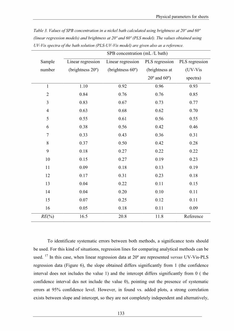
Table 3. Values of SPB concentration in a nickel bath calculated using brightness at 20º and 60º
(linear regression models) and brightness at 20º and 60º (PLS model). The values obtained using
UV-Vis spectra of the bath solution (PLS-UV-Vis model) are given also as a reference.
SPB concentration (mL /L bath)
Sample
number
Linear regression
(brightness 20º)
Linear regression
(brightness 60º)
PLS regression
(brightness at
20º and 60º)
PLS regression
(UV-Vis
spectra)
1 1.10 0.92 0.96 0.93
2 0.84 0.76 0.76 0.85
3 0.83 0.67 0.73 0.77
4 0.63 0.68 0.62 0.70
5 0.55 0.61 0.56 0.55
6 0.38 0.56 0.42 0.46
7 0.33 0.43 0.36 0.31
8 0.37 0.50 0.42 0.28
9 0.18 0.27 0.22 0.22
10 0.15 0.27 0.19 0.23
11 0.09 0.18 0.13 0.19
12 0.17 0.31 0.23 0.18
13 0.04 0.22 0.11 0.15
14 0.04 0.20 0.10 0.11
15 0.07 0.25 0.12 0.11
16 0.05 0.18 0.11 0.09
RE(%) 16.5 20.8 11.8 Reference
To identificate systematic errors between both methods, a significance tests should
be used. For this kind of situations, regression lines for comparing analytical methods can be
used. 17
In this case, when linear regression data at 20º are represented versus UV-Vis-PLS
regression data (Figure 6), the slope obtained differs significantly from 1 (the confidence
interval does not includes the value 1) and the intercept differs significantly from 0 ( the
confidence interval des not include the value 0), pointing out the presence of systematic
errors at 95% confidence level. However, in found vs. added plots, a strong correlation
exists between slope and intercept, so they are not completely independent and alternatively,

Physical parameters for sheets
134
the test of the confidence ellipse can be applied to find systematic errors.18,19
In this case, the
test of the ellipse (not shown) confirmed the existence of systematic error.
Figure 6. Looking for systematic errors in SPB determination with a linear regression model
(brightness data at 20º). Found vs. added plot is shown with slope and intercept given with a
confidence interval of 95%. Data obtained with the UV-Vis-PLS calibration model are used as a
reference (x-axe).
The use of brightness at 60º did not change the results; that is, systematic errors do
probably exist. It was said above that brightness at 20º is more discriminant during the first
sheets of the bath, whereas brightness at 60º is more informative at longer stages. To use the
information of brightness at both angles, a PLS calibration model using brightness data at
both angles (20º and 60º, 12 points per sheet) was developed instead. In this case, lower
errors for both calibration and validation samples were obtained, compared with the simple
regression lineal methods (Table 2). For an external further validation, the PLS model was
applied to the same sheets of the old bath. Results are given in Table 3 together with those
previously obtained for the linear regression model that used brightness either at 20º or 60º.
To find systematic errors (significant difference with UV-Vis-PLS results), similar tests to
those previously used were tried again and the result are given in Figure 7.
slope = 1.154±0.041
intercept = -0.079±0.019
r= 0.98
0
0.6
1.2
0.0 0.5 1.0
mL SPB added/L Bath
mL
SP
B fo
und/
L B
ath

Physical parameters for sheets
135
Figure 7. Tests to find systematic errors when the PLS model (brightness data at 20º and 60º) is used
for calibration. The PLS model that uses UV-Vis-data from the bath solution is used as a reference.
(a) In the found vs. added plot the slope and intercept are given with a confidence interval of 95(%).
(b) Test of the joint confidence ellipse (P = 0.05) for data in (a).
In this case, the confidence intervals (P = 0.05) include the values 1 (slope) and 0 (intercept)
(Figure 7a); on the other hand, in the ellipse test for P = 0.05, the point that represent slope
and intercept stands inside the ellipse showing tat systematic errors have not been proven to
exist.
As a conclusion, it can be said that both brightness at 20º and 60º are necessary to assure
good predicting results. Brightness of plated sheets can, then, be used to determine the SPB
concentration in a nickel bath, provided that a PLS model has been built. This should be
considered as a promising alternative to other precedent methods to determine the brightener
(additive) concentration in a simple, fast and easy way.
6.3.2. Exploring of sheets images through PCA
Desktop flatbed scanners are present in most laboratories as a part of the computer
support and can provide digitized information of flat surfaces. The information obtained
with a scanner from a flat surface can be used with fine results for exploratory purposes
through image analysis.
0.816
1.072
-0.029 0.0604
(b)
intercept
slop
e
(a)
slope = 0.946±0.035
intercept = 0.016±0.017
r= 0.98
0
0.5
1
0 0.5 1
mL SPB/L bath added
mL
SP
B/L
bat
h fo
und
Physical parameters for sheets
136
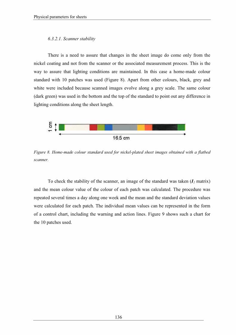
6.3.2.1. Scanner stability
There is a need to assure that changes in the sheet image do come only from the
nickel coating and not from the scanner or the associated measurement process. This is the
way to assure that lighting conditions are maintained. In this case a home-made colour
standard with 10 patches was used (Figure 8). Apart from other colours, black, grey and
white were included because scanned images evolve along a grey scale. The same colour
(dark green) was used in the bottom and the top of the standard to point out any difference in
lighting conditions along the sheet length.
Figure 8. Home-made colour standard used for nickel-plated sheet images obtained with a flatbed
scanner.
To check the stability of the scanner, an image of the standard was taken (I1 matrix)
and the mean colour value of the colour of each patch was calculated. The procedure was
repeated several times a day along one week and the mean and the standard deviation values
were calculated for each patch. The individual mean values can be represented in the form
of a control chart, including the warning and action lines. Figure 9 shows such a chart for
the 10 patches used.

Physical parameters for sheets
137
Figure 9. Control chart for the use of the flatbed scanner. The colours in Figure 8 are represented.
The mean colour value in each case, together with the warning (±2s) and action (±3s ) lines, is
shown.
This provides information to assess if there is any change in lighting conditions.
Whenever a plated sheet is scanned, an image of the 10 patches standard is also taken (I2
matrix). If the mean channel value of every colour in the patch stands within the action lines,
no correction is necessary; otherwise, a correction should be performed.
To make a correction it should be considered that the original standard images (I1, I2,
etc.) are formed by m pixels, but once they are transformed to the RGB model and unfolded,
they form a matrix of m columns (the number of pixels) and 3 files (the RGB colours); that
is, any of those matrices can be represented by I(m,3) . Bold characters represent matrices and
superscript T means the transpose. The dimensions of matrices are given as a subscript. To
correct I2(m,3) into I1(m,3) , when necessary, the matrix M(3,3) must be obtained:20
1(m,3)(3,3)2(m,3) IMI =⋅ (3)
The correction can be expected to conform to a linear model and then:
2(m,3)m1(3,1(m,3)m)1(3,(3,3) II]I[IMT
)
1T ⋅⋅= − (4)

Physical parameters for sheets
138
Once )3,3(M is known, it can be applied to correct the image of the corresponding
nickel sheet, regardless the number of pixels. If the sheet image, transformed and unfold, is
represented by )3,(2 nP (n pixels), the corrected image will be represented by:
)3,3()3,(2)3,(1 MPP ⋅= nn (5)
The image 1(n,3)P can be compared with any other sheet image either obtained under
stable lighting conditions or corrected according to equation (3). Obviously, the matrix
M(3,3) in Eq. (2) changes for each sheet whenever )3,(2 mI differs significantly from I1(m,3)
owing to changes in lighting conditions. If they are stable, )3,3(M is the unity matrix.
During the work, the lighting conditions were kept mostly stable and no correction
was performed.
6.3.2.2. Acquisition of the RGB image. Sheets scanning
An amount of 53 sheets were consecutively plated before the bath was considered to
have run out. Images were then obtained for every sheet and the colour standard was always
included. Figure 10 shows the scanned images of the whole set. The first sheets, highly
bright, look mainly black, whereas the last ones are mainly grey. This evolution could also
be appreciated at first glance, with no need of scanning, but it would be helpful to establish
an objective technique capable of measuring the plating evolution by a colour scale.
If the images in Figure 10 are decomposed into the RGB channels, the evolution, for
instance in the red channel, can clearly be appreciated (Figure 11). The blue colour
dominates in the first sheets, whereas orange dominates in the last ones. The colour
evolution is first appreciated in the centre of each sheet as it can be seen from Figure 11.
This is due to the apparition of a dull-stripe that grows up from the centre to the corners and
it is indicative of the loss of brightness. The stripe size can be related to the sheet quality
because samples with a wide and white stripe would not be industrially accepted. The reason
for this effect is that the nickel electrodeposition is not a homogeneous process. The loss of

Physical parameters for sheets
139
brightness quality is firstly appreciated in the centre of the sheets because the density of
current is, in general, lower in the centre than in the corners.
The evolution can also be appreciated in a different way when the image of the
whole plate is represented as a histogram of colour frequency vs. the colour value in the
RGB space. Figure 12 shows that kind of plot for the whole set of sheets. The important
parameters are the more frequent colour value and the spread of histogram. Narrow
histograms mean homogeneity in the brightness level, whilst wide histograms represent lack
of homogeneity in the brightness level. Low colour values indicate finely-plated sheets (blue
colour) and high colour values are related to poorly-plated sheets (orange colour).

Physical parameters for sheets
140
y-l
ength
5
cm
x-length
3.75 cm
Figure 10. Scanned images of the electroplated sheets of a
whole run. The sheet number is given above.

Physical parameters for sheets
141
Figure 11. RGB images for the electroplated sheets in
Figure 10. The sheet number is given above. The colour
scale is given in each case.
x-length
3.75 cm
y-l
ength
5
cm

Physical parameters for sheets
142
Mean colour value
Figure 12. Histograms for the electroplated sheets in Figure 10.
The sheet number is given above.
Colo
ur
freq
uen
cy

Physical parameters for sheets
143
6.3.2.3. PCA of the sheet images.
A more precise look at the whole coating transition can be obtained when PCA
analysis is applied to the unfolded images of the whole data set. The procedure was followed
in order to see if significant differences between the two faces could be found, to find out
the directions of maximum variability and to identify odd samples (outliers). PC1 accounts
for a data variability of 96.46%, whereas PC2 explains 0.75% and PC3 only a residual
0.09%. No significant differences were found between the two faces of the sheet (Figure
13), indicating that stirring during electrodeposition was efficient. From now on, and in
order to simplify the data handling, only “A face” samples will be considered.
Figure 13. PC1 and PC2 scores for A (▼) and B (○) faces. Red-channel data.
PC1 explains most of the information, and it is the main indicator of the sheet
brightness quality evolution. Figure 14a shows how the PC1 score increases with the sample
number, after a short induction period, and this is related to the fact that deposits go from
being totally glossy-bright to completely grey. The values of PC2 scores are shown in
Figure 14b. There is a “W” shape that seems to be related to the lack of uniformity in the
brightness levels of deposits and the appearance of a dull-centre-stripe in the sheets as the
bath is run out. Highly-bright, medium-bright or totally light-grey sheets (homogenous

Physical parameters for sheets
144
aspect in any case) are characterized by a high-score value and by a narrow histogram and
are distributed at the top of the graph. Sheets that are medium-bright in its central part and
highly-bright in the corners or grey in its central part and medium-bright in the corners (non-
homogeneous) are distributed at the bottom of the graph because of their low score value
and are characterised by a wide histogram. These results are confirmed when the loadings
from the two first PC are taken into account. Figures 14c and 14d show the loadings of PC1
and PC2 respectively, rearranged into images that remind of a contour diagram. The colour
intensity of every pixel (represented in the colour scale attached) is zenithally projected onto
the plane where the different pixels are represented. Red colour is assigned to high loading
values and it means that the pixel bears relevant information; blue colour indicates low
values of loading, which means pixels with irrelevant information. The loadings from PC1
and PC2 confirm that the central part of the sheet is the most sensible to the loss of
brightness quality (Figure 14) and the numerical value of the loading is higher in that region.

Physical parameters for sheets
145
Figure 14. PC1 (a) and PC2 (b) scores as a function of the sheet number. (c) and (d) are the
loadings of the corresponding scores for image data. In (a) and (b) filled rhombs correspond to
image data and open circles to specular reflectance data.
6.3.2.4. Specular reflectance (SR) and critical evaluation
In specular reflectance (SR) the light from a source impinges on the sample and the
reflected light is measured at a prefixed angle. The wavelength range of the incident light
depends on the source (180-900 nm in this case) and a complete spectrum of reflected light
can be obtained if a spectrophotometer is used. The intensity of the signal will depend on the
material and on the angle of illumination. In this case, spectra were registered at 90º.
Physical parameters for sheets
146
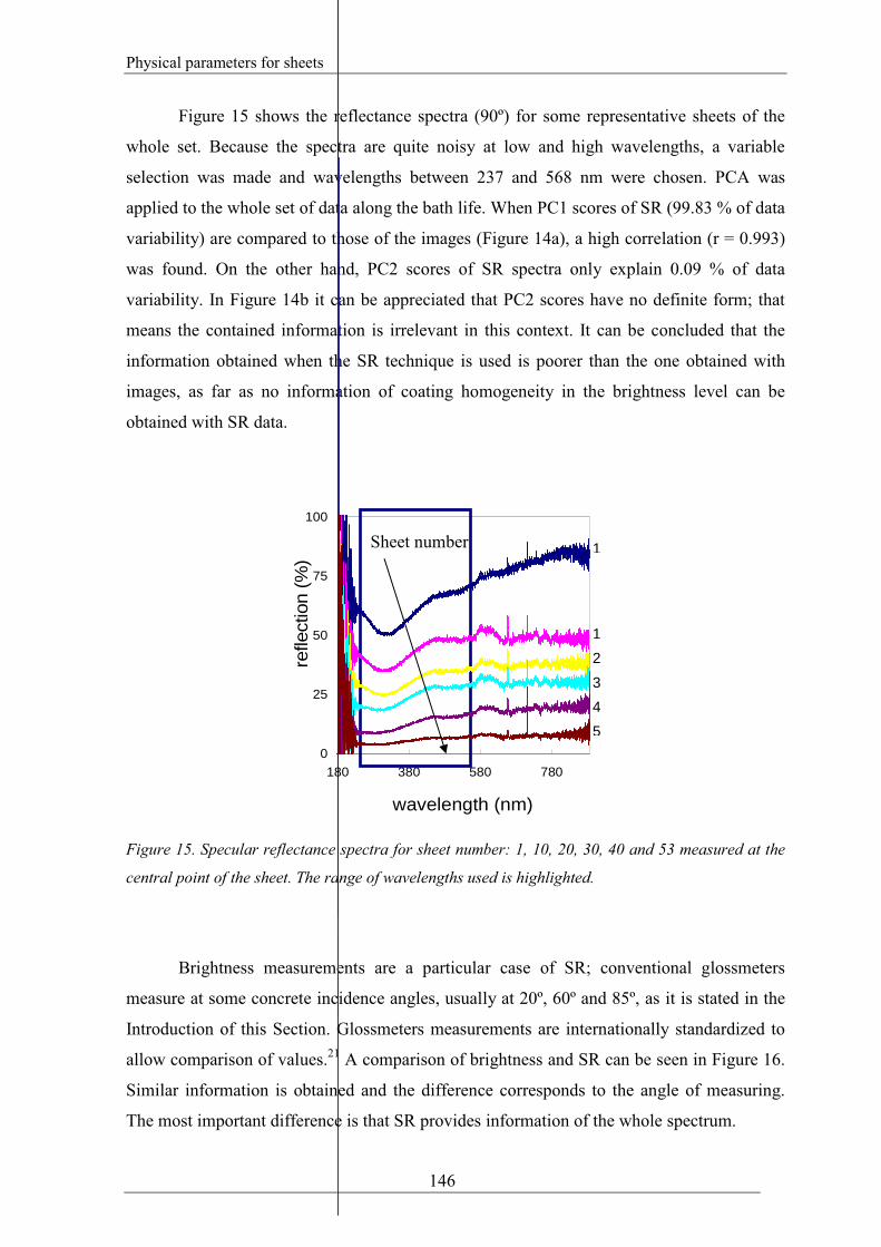
Figure 15 shows the reflectance spectra (90º) for some representative sheets of the
whole set. Because the spectra are quite noisy at low and high wavelengths, a variable
selection was made and wavelengths between 237 and 568 nm were chosen. PCA was
applied to the whole set of data along the bath life. When PC1 scores of SR (99.83 % of data
variability) are compared to those of the images (Figure 14a), a high correlation (r = 0.993)
was found. On the other hand, PC2 scores of SR spectra only explain 0.09 % of data
variability. In Figure 14b it can be appreciated that PC2 scores have no definite form; that
means the contained information is irrelevant in this context. It can be concluded that the
information obtained when the SR technique is used is poorer than the one obtained with
images, as far as no information of coating homogeneity in the brightness level can be
obtained with SR data.
Figure 15. Specular reflectance spectra for sheet number: 1, 10, 20, 30, 40 and 53 measured at the
central point of the sheet. The range of wavelengths used is highlighted.
Brightness measurements are a particular case of SR; conventional glossmeters
measure at some concrete incidence angles, usually at 20º, 60º and 85º, as it is stated in the
Introduction of this Section. Glossmeters measurements are internationally standardized to
allow comparison of values.21
A comparison of brightness and SR can be seen in Figure 16.
Similar information is obtained and the difference corresponds to the angle of measuring.
The most important difference is that SR provides information of the whole spectrum.
0
25
50
75
100
180 380 580 780
wavelength (nm)
refle
ctio
n (%
)
1
1
2
3
4
5
Sheet number

Physical parameters for sheets
147
0
250
500
0 20 40
current (A·h/L)
Brig
thne
ss
0
20
40
Spe
cula
r R
efle
ctan
ce (
%)
( λ =
300
nm
)
brigthness 20ºbrigthess 60ºSR (300 nm)
Figure 16. Comparison of brightness at 20º (•), brightness at 60º (ο) and SR at 90º (∗).
Both image analysis and SR provide similar information on brightness quality of the
plating process. The interpretation of SR original data is easier, but image analysis with
flatbed scanners provides a great amount of information of the entire sheet surface, whereas
SR only provides information on a few points of the sheet; consequently, irregularities or
lack of brightness homogeneity on the surface can be found with scanners but not with SR
measures. Measurements are more easily taken with a scanner and a much better
reproducibility is obtained. Finally, a general purpose scanner can amount to about 50€, but
SR measures need instrumentation for at least 100-fold.
6.3.3. Additive control by image analysis
6.3.3.1. Mean colour value (MCV)
The MCV of the red channel of the 53 electroplated sheets (Figure 11) was
calculated (Figure 17). The internal standard was always included, but no need of colour
correction was necessary ever. These MCV together with its corresponding standard
deviation values are depicted in Figure 17.

Physical parameters for sheets
148
Figure 17. Mean colour value of the red channel (points) and standard deviation (bars) of the
samples of Figure 11.
The colour value increases with the age of bath as long as sheets loss brightness
quality. The standard deviation is lower for both the first and the last few electroplated
sheets, and is larger for the halfway sheets.
If the MCV is compared to the PC1 scores of image, (Figure 18), it can be been seen
that both of them follow a very similar pattern. The correlation was found to be 1.000. They
are, hence, completely correlated. As PC1 explains most of the information, and it is the
main indicator of the sheet brightness quality evolution it can be said that just a number (the
mean colour value) can be used to represent every sheet. Therefore, the MCV can be used as
an estimation of the age of the bath becoming useful to discriminate if sheets are suitable or
not for industry purposes. Also, MCV is able to determine the brightness quality of sheets as
a whole. Nonetheless, the first symptom of bath aging is a white, not glossy, central stripe
(Figure 10). Because of this, the standard deviation of the MCV could also be related to the
brightness quality of deposits.
Sheet number
Mea
n co
lour
val
ue

Physical parameters for sheets
149
20
70
120
170
0 20 40
sheet number
mea
n co
lour
val
ue
-200
-100
0
100
200
PC
1 sc
ores
(im
age
PC
A)
-25
0
250 20 40
sheet number
PC
2 sc
ores
5
25
45
stan
dard
dev
iatio
n
Figure 18. Correlation between mean colour values (●, filled circles) and PC1 image scores (○,
open circles).
In Figure 19 it is seen how the standard deviation of MCV is correlated to the PC2
values (r = 0.71). Consequently, the calculated standard deviation could be used as an
additional parameter to evaluate the sheet homogeneity, as it was seen with PC1 scores. In
general, the deposit on a sheet with low standard deviation value is more homogeneous than
that of a sheet with a high standard deviation value. A different thing is if they are brilliant
or not: in Figure 11, sheet 1 is homogeneous (small standard deviation) and brilliant,
whereas sheet 53 is homogeneous (small standard deviation), but not brilliant at all.
Figure 19. Correlation between PC2 scores (filled circles) and standard deviation of the mean
colour value (bars).

Physical parameters for sheets
150
6.3.3.2. Sheets classification and brightness quality assessment
The 53 plated sheets (Figure 10) were evaluated by a group of experts (from
CIDETEC)22
and classified into 5 different quality groups. The classification was made
subjectively, depending on their external appearance and it is summarized in Table 4. As a
reference, the first electroplated sample was taken as the sheet with the maximum possible
quality, since the bath was considered to be in the best conditions for electroplating.
Table 4. Sheets assessment based on their external appearance.
The difference between group 1 and group 2, EQ and GQ respectively, is due to the
apparition of a central dull stripe. However, the assessment concluded that the sheets
belonging to the two first groups, EQ and GQ, could be considered suitable for the
decorative industry of nickel, while sheets from MQ to VBQ would not have the minimum
quality associated to a bright nickel bath.
Group Sheet number Quality Characteristics
1 1-11 Excellent quality
(EQ)
High-bright sheets.
2 12-22 Good quality
(GQ)
Bright sheets. A dull stripe grows up
from the centre to the corners of the
sheet.
3 23-33 Medium quality
(MQ)
Semi-bright sheets. The dull band
covers practically the entire sheet.
4 34-44 Bad quality
(BQ)
Low-bright sheets. A white-band
grows up from the centre to the corners
of the sheet.
5 45-53 Very bad quality
(VBQ)
Very low-bright sheets. Almost
completely covered in white.

Physical parameters for sheets
151
As it has been stated above, each sheet could be characterized by a single number,
the mean colour value, as it is the main indicator of the sheet brightness quality evolution.
Therefore, the classification between groups will stay as it is given in Table 5 and Figure 20.
Table 5. Sheet assessment depending on their colour mean value.
Figure 20. Mean colour value (circles) and standard deviations (bars). Horizontal red lines indicate
the group separation, depending on the quality assignment made by the experts.
If a number is assigned to the nickel deposit brightness quality, it can be used to take
decisions on the bath composition (addition of additives, etc.).
Quality Range of the mean colour value
EQ 0- 50
GQ 51-102
MQ 103-126
BQ 127-158
VBQ 159-255
MQ
EQ
GQ
BQ
VBQ
Sheet number
Mea
n co
lour
val
ue

Physical parameters for sheets
152
6.3.3.3. Calibration models for additives
If MCV is related to the physical aspect of the sheets, that is, to the quality of the
coating, some relation should exist with the additives concentration, especially to those that
modify their concentration along the bath life.
Figure 21 shows the relation of MCV to the SPB and SA-1 concentrations. In order
to determine the SPB and SA-1 concentrations from MCV, a calibration graph should be
deduced from plots in Figure 21a and Figure 21b. No simple calibration model was found to
relate MCV and SPB concentration, so it was decided to use an empiric model that should
be validated with external samples from a different plot. After some tries, it was decided to
use a quadratic relation by stretches, any of them covering ten sheets. The last stretch, that
covered thirteen sheets, was not considered because it had no use. Table 6 shows the
quadratic equations and the stretches covered.
Figure 21. Evolution of the mean colour vale with the additives concentration during an
electroplating process. (a) additive SPB; (b) additive SA-1.
25
75
125
175
-0.05 0.30 0.65 1.00
mL SPB/L bath
mea
n co
lour
val
ue
(a)
25
75
125
175
0.5 1.25 2 2.75
mL SA-1/L bath
mea
n co
lour
val
ue
(b)

Physical parameters for sheets
153
Table 6. Equations used to model the SPB concentration (in mL/L) as a function of MCV and intervals of
application.
SPB = a2 · (MCV) + b · (MCV) + c
Stretch number Sheet interval a b c
1 1-10 3.3·10-3
-0.28 6.5
2 11-20 6.2·10-5
-0.013 0.87
3 21-30 5.0·10-5
-0.017 1.37
4 31-40 2.0·10-5
-0.008 0.72
The equation used to relate the SA-1 concentration and MCV was:
SA-1 (mL/L) = -0.010 MCV + 2.68 (r = 0.91) (6)
The calibration models obtained were used to calculate the SPB and SA-1
concentrations that should be added to the nickel bath to recover the initial electroplating
conditions. In the new nickel bath, the MCV of any electroplated sheet was calculated and
SPB and SA-1 concentrations were deduced as a result.
No calibration models were built for A-5(2X) and NPA because A-5(2X) keeps
unchanged during the electroplating process (determined by UV-Vis, see Section 4) and
NPA gave very imprecise results (determined by NMR, see Section 5).
6.3.3.4. Real-control and bath quality maintenance
A new software was programmed in Matlab in order to follow the concentrations of
SPB and SA-1 through MCV of the electroplated sheets. A total amount of 103 sheets was
now plated and additives were added whenever necessary, according to the above-
mentioned calibration models. The aim was to maintain the nickel bath in conditions good
enough to obtain deposits of EQ and GQ quality (Table 5) at any time.
The following values must be introduced as input in the software, whenever a new sheet is
going to be plated:
1) The time of electroplating per sheet.

Physical parameters for sheets
154
2) The original concentration of SPB additive (in the nickel bath).
3) The original concentration of SA-1 additive (in the nickel bath).
4) The volume of nickel bath in the vessel for electrodeposition.
Thus, the values in this study that were introduced everytime were:
1) 15 minutes
2) 1mL L-1
bath
3) 2.6 mL L-1
bath
4) 1.8 L
The following output are obtained:
- The MCV of each patch in the colour standard.
- The histogram of the plated sheet.
- The MCV of the plated sheet.
- The standard deviation value of the plated sheet.
Depending on the MCV obtained, each sheet is classified into one of the 5 quality
groups established by the sensorial panel (Table 4). When a sheet is classified from MQ to
VBQ (sheets not industrially accepted), it is considered that some feeding of the bath with
SPB and SA-1 is neccesary. Then, the amount in mL L-1 bath of both additives that should
be added to obtain accepted plating is given.
Figure 22 depicts the Real-control output after the electrodeposition of the first sheet.
The output comprises four different plots. (a), red-channel image of the sheet scanned; (b),
the histogram of the sheet scanned (c), the MCV for the sheet scanned (quality sensorial
limits are given by red discontinuous lines) and (d), the standard deviation of the colour
frequency. Standard deviations below 10 are considered low; the sheet is, then,
homogeneous. Standard deviations above 15 are considered high and the sheet is, then, non-
homogeneous (upper and lower limits are given by red-discontinuous lines). The MCV is
used as an analytical signal to calculate the amounts of SPB and SA-1 to be added. The
histogram and the standard deviation are used as assessment factors. The blue colour
dominates in sheet image. The histogram is narrow and standard deviation is low. All of
Physical parameters for sheets
155
them are indicators of high brightness quality deposits. The mean colour value is small as
well and keeps inside EQ group.
Figure 22. Real-control result for the first electroplated sheet.
Figure 23 represent the Real-control output for a complete batch before any additive
reefed and Figure 24 represents the same output after bath feeding with SPB and SA-1.
Before additives feeding, 30 sheets had been electroplated. Along the process, quality was
lowering as expected. The first 13 sheets showed an excellent quality as they belong to the
EQ group. Sheets from number 14 to number 29, with lower brightness quality, belong to
the GQ group and sheet number 30 to the MQ group. That is, the quality is not adequate any
more and both, SPB and SA-1 must be added in order to take the bath back to the initial
optimum electroplating conditions. The software automatically outputs the SPB and SA-1
volumes (in mL) to be added. Sheets number 12 and 15 reveal a high standard deviation
value. This was probably due to the fact that these sheets were not properly plated, as the
plating showed excessively pitted. It could be attributed to a bad-state of the sheet surfaces
before plating or to a poor clean up of the sheets before electrodeposition.
VBQ
MQBQ
GQ
EQ
(a) (b)
(c)
(d)
Physical parameters for sheets
156
Figure 23. Real-control result after first complete batch and before additives replenishment (sheet
number 30);
Figure 24. Real-control result after first complete batch after additives replenishment (sheet
number 31).
(a) (b) (d)
(c)
VBQBQ MQGQ
EQ
(a) (b) (d)
(c)
VBQBQ MQGQ
EQ

Physical parameters for sheets
157
Once the additive replenishment has been accomplished and the sheet number 31 is
scanned, Figure 24 is obtained. The difference between the two outputs is significant,
especially when plots (a) and (b) are considered. Sheet number 30 is characterized by a red-
colour stripe in the middle of the image, a wide histogram and a high value of the standard
deviation. On the other hand, sheet number 31 is characterized by a blue-colour image, a
narrow histogram and a low value of the standard deviation; all that means an excellent
brightness quality coating. If the output in Figure 24 is compared to the output in Figure 22,
at the beginning of the whole process, it can be seen how the initial conditions are
recovered.
As it was said, the entire electrodeposition process consisted of 103 sheets. In Figure
25 the Real-control result after scanning the sheet number 103 is depicted. This includes
three entire batches and the beginning of the fourth. The initial quality is recovered at the
end of each batch. Furthermore, the length of each batch is similar in every case, indicating.
that the additive consumption is the main factor affecting the bath life.
The volume of additives added at the end of each batch is registered in Table 7.
Figure 25. Real-control result for the whole electroplating process after several batches. The last
sheet scanned is pointed out in each case.
(a)
VBQ
BQ MQ
GQ
EQ
(b) (d)
(c)

Physical parameters for sheets
158
Table 7. Volumes of SPB and SA-1 added at the end of each batch.
* calculated for 1.8 L of nickel bath.
6.3.3.5. Reference techniques
The A-5(2X) and SPB evolution during electrodeposition process was checked by
independent analytical techniques.
6.3.3.5.1. UV-Vis spectrophotometry
Aliquots were regularly taken from the bath by a manual way, UV-Vis spectra were
acquired and the PLS calibration matrix described for the manual procedure in section
4.2.4.2. was applied to find de additives concentration in the solution where the sheets had
been coated.
The evolution of both additives is depicted in Figure 26. The A-5(2X) concentration
keeps approximately constant, as already established. The SPB concentration follows the
well-known first order decay. In this case, the points where the additive was added are
pointed out.
Sheet number mL SPB added* mL SA-1 added*
Batch 1 30 1.62 2.00
Batch 2 64 1.47 1.75
Batch 3 95 1.58 1.93

Physical parameters for sheets
159
Figure 26. Evolution of (a) A-5(2X) and (b) SPB concentrations along the whole process, that
embodied three entire batches and the beginning of the fourth one. Points of refeeding have been
marked.
The SPB concentration can be calculated with good accuracy after every addition.
Table 8 compares the volumes of SPB added, dictated by the Real-control program, and the
volumes found with the manual UV-Vis method, (Figure 26b). In both cases, the initial
conditions of the bath were taken as a reference, because the quality is then optimum for
electrodeposition. The last column of Table 8 shows the errors calculated in the volume
-0.1
0.3
0.7
1.1
0 20 40
current (A·h/L)
mL
SP
B/L
Bat
h
SPB and SA-1 refeed (b)
0
10
20
30
0 20 40current (A·h/L)
mL
A-5
(2X
)/L
Bat
h
(a)

Physical parameters for sheets
160
added when the UV-Visible method is considered as a reference. The accuracy found ranged
between 0.6 and 13%, which can be considered an excellent result, taking into account that
image analysis is a less time-consuming technique. Moreover, it is less invasive and less
expensive and cheaper than UV-Vis spectrophotometry.
Table 8. Volume of SPB calculated by image analysis (with real-control software) and by UV-Vis
spectrophotometry.
6.3.3.5.2. Brightness
Similarly to UV-Vis spectra, brightness of the sheets along the batches was also
measured. Both brightness at 20º and 60º were registered as it is explained in Section
6.2.4.1., and the PCA algorithm was applied. Figure 27 shows the PC1 scores of brightness
data together with the SPB concentration along the batches (UV-Vis data). There is a high
correlation between both kind of data (r =0.998) as it could be expected since it was
demonstrated that they can be predicted from each other.
mL SPB added
(image analysis)
mL SPB found
(UV-Vis spectrophotometry)
error(%)
Batch 1 1.62 1.61 0.6
Batch 2 1.47 1.68 -13.1
Batch 3 1.58 1.66 -4.8
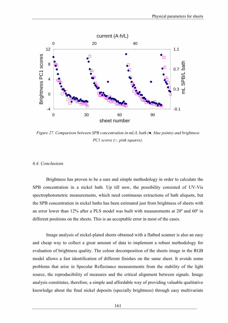
Physical parameters for sheets
161
-4
0
4
8
12
0 30 60 90
sheet number
Brig
htne
ss P
C1
scor
es
-0.1
0.3
0.7
1.10 20 40
current (A·h/L)
mL
SP
B/L
bat
h
Figure 27. Comparison between SPB concentration in mL/L bath (●, blue points) and brightness
PC1 scores (□, pink squares).
6.4. Conclusions
Brightness has proven to be a sure and simple methodology in order to calculate the
SPB concentration in a nickel bath. Up till now, the possibility consisted of UV-Vis
spectrophotometric measurements, which need continuous extractions of bath aliquots, but
the SPB concentration in nickel baths has been estimated just from brightness of sheets with
an error lower than 12% after a PLS model was built with measurements at 20º and 60º in
different positions on the sheets. This is an acceptable error in most of the cases.
Image analysis of nickel-plated sheets obtained with a flatbed scanner is also an easy
and cheap way to collect a great amount of data to implement a robust methodology for
evaluation of brightness quality. The colour decomposition of the sheets image in the RGB
model allows a fast identification of different finishes on the same sheet. It avoids some
problems that arise in Specular Reflectance measurements from the stability of the light
source, the reproducibility of measures and the critical alignment between signals. Image
analysis constitutes, therefore, a simple and affordable way of providing valuable qualitative
knowledge about the final nickel deposits (specially brightness) through easy multivariate
Physical parameters for sheets
162
PCA analysis. This can help industries to take decisions on the suitability of nickel bath
conditions. The quantitative power of the technique for analysis of the bath has been also
considered through a new software implemented in MatLab, named Real-control. The
application has demonstrated to be a helpful and reliable technique in order to extract
information from the scanned sheets. This information can be used as a brightness quality
assessment on the electroplated sheets. If the mean colour value of sheets is employed, the
concentrations of SPB and SA-1 additives can be kept into optimum levels as they are added
when necessary. Thus, an effective and successful electrodeposition process can be assured.
UV-Vis spectrophotometry and brightness measurements have been used as reference
techniques to follow the concentration of SPB in the bath along the procedure as reference
techniques.

Physical parameters for sheets
163
6.5. References
1 G. A. Dibari, Plat. Surf. Finish., 2000, 87, 50-53.
2 J.W. Böcker, T. Bolch, A. Gemmler, P. Jandik, Plat. Surf. Finish, 1992, 79, 63-69.
3 C.C. Hu , C.Y. Lin, T.C. Wen, Mater. Chem. Phys., 1996, 44, 233-238.
4 V. Darrort, M. Troyon, J. Ebothé, V. Bissieux, C. Nicollin, Thin Solid Films, 1995, 265,
52-57.
5 S. Chakraborty, T. Met. Finish. India, 2003, 12, 123-133.
6 D.W. Baudrand, Plat Surf Finish, 2007, 94, 32-36.
7 N.V. Mandich , H. Geduld, Metal Finishing, 2002, 100, 83-91.
8 J. W. Dini, Electrodeposition, Noyes Publications, New Jersey, 1993, 206.
9 http://www.gloss-meters.com/ (last accessed in march 2010).
10 H.E. Bennett, J.O. Porteus, J. Opr. Soc.Am., 1961, 51(2), 123-129.
11 P. Facco, F. Bezo, M. Barolo, R. Mukherjee, J.A. Romagneli, Am. Chem. Eng., 2009, 55,
1147-1160.
12 J.C. Russ, Image Analysis of food microstructure, CRC Press, Florida, 2005, 71-77.
13 H. Shinzawa, K. Awa, W. Kanematsu, Y. Ozaki, J. Raman Spectrosc., 2009, 40, 1720-
1725.
14 Y.L. Shishkin, S.G. Dmitrienko, O.M. Medvedeva, S.A. Badakova, L.N. Pyatkova, J.
Anal. Chem., 2004, 59, 102-106.
15 S.P. Yadav, Y. Ibaraki, S. Dutta Gupta, Plant. Cell. Tiss. Organ.Cult., 2010, 100, 183-
188.
16 E. Gebel, Anal. Chem., 2010, 82, 764-765.
17 J. N. Miller, J. C. Miller, Statistics and Chemometrics for Analytical Chemistry, 5
th ed.,
Pearson Education Limited, Harlow, England, 126-131.
18 J. Mandel, F.J. Linning, Anal Chem., 1957, 29, 743.
19 R. Boqué, F. X. Rius, Avances en quimiometría práctica. Universidad de Santiago de
Compostela, 1994, 176.
20 G.Y. Tian, D. Gledhill, D. Taylor, D. Clarke, Proceedings of the Sixth International
Conference on Information Visualization, IV’02, 2001, 483-488.
21 http://www.iso.org/
22 CIDETEC, Centro de Tecnologías Electroquímicas, San Sebastián, Spain.

7. Abstract and Conclusions

General conlusions
167
The behaviour of a nickel bath has been studied along an electrodeposition
process by different analytical and chemometrics tecniques.
First of all, it was checked that the concentrations of Ni2+ and Cl
- keep constant
during the whole bath life. This was made by absorbance measures and by
argentometric titrations respectively. The value of pH must be maintained around 4.5
with the addition of H2SO4. On the other hand, the working temperature of the bath
must be kept within the 60-70ºC range and it was accomplished by a water bath
thermostat.
Secondly, the control of additives was accomplished by different analytical
techniques. UV-Vis spectrophotometry proved to be a suitable technique to follow the
evolution of A-5(2X) and SPB additive concentrations in a nickel bath. No systematic
errors were found in the determination of both additives. The procedure was
accomplished either by an automatic bath sampling (SI-system) or by a manual
procedure, used as a reference technique. The implementation of the SI-system is easy
and cheap, and not sophisticated apparatus are needed. This can be very interesting from
an industrial point of view. Multivariate methods of calibration were applied due to the
spectral overlapping. Both PLS and CLS models can be used for monitoring the
additive degradation along the life of the bath. Nevertheless, the best prediction results
are obtained by using PLS with first derivative experimental data.
NMR has also proven to be a suitable technique in order to follow the evolution
of all the additives in the bath (A-5(2X), SPB, SA-1 and NPA) provided that nickel ions
are previously separated by precipitation with NaOH. In this case, univariate and
multivariate methods can be applied and both methodologies gave good results, but the
best predictions were obtained when PLS regression is applied. Additives conversion
into degradation products can be also appreciated as long as peaks of additives decrease
and new peaks arise along the electroplating process. An important characteristic of
multivariate techniques is the fact that normalization vs. internal standard is not an
essential task for quantitation and this is an important advantage for complex and
crowded spectra.

General Conclusions
168
It has been found that the level of SPB in the bath follows a first-order decay
model. SA-1 also decreases along the electrodeposition but A-5(2X) and NPA, keep
approximately constant. The study of the peaks evolution by NMR suggested that at
least a new compound is formed and it probably comes from the degradation of SA-1.
Physical parameters have been also assessed in the final product of the
electrodeposition by the use of techniques such as brightness, specular reflectance and
image analysis. Brightness proved to be a sure and simple methodology in order to
calculate the SPB concentration in a nickel bath. It can be estimated with an error lower
than 12% when a PLS model is built with measurements at 20º and 60º in different
positions on the sheets. This can be considered as an acceptable error in most of the
cases. Image analysis of nickel-plated sheets obtained with a flatbed scanner has
constituted a simple and affordable way of providing valuable qualitative knowledge
about the final brightness quality through easy multivariate PCA analysis. The colour
decomposition of the sheets image in the RGB model allows a fast identification of
different finishes on the same sheet and some problems of specular reflectance such as
stability of the light source, reproducibility of measures and critical alignment between
signals are avoided. This can help industries to take decisions on the suitability of nickel
bath conditions. The quantitative power of the technique for analysis of the bath has
been also considered through a new software implemented in MatLab, named Real-
control. The application has demonstrated to be a helpful and reliable technique in order
to extract information from the scanned sheets. This information, allows the control of
the brightness quality on the electroplated sheets and tells the amount of SPB and SA-1
additives to be added into the bath, so that optimum levels of these additives are
maintained.

8. Resumen y Conclusiones


Resumen y conclusiones
171
Diversas técnicas analíticas y la quimiometría como herramienta han permitido
estudiar el comportamiento de un baño de níquel durante el proceso de
electrodeposición.
Inicialmente, se comprobó mediante medidas de absorbancia y mediante
valoraciones argentométricas el comportamiento de las concentraciones de Ni2+ y Cl
-
del baño. Ambos parámetros se mantienen aproximadamente constantes durante el
proceso de electrodeposición. Además, se hicieron adiciones puntuales de H2SO4 para
mantener el pH del baño en torno a 4.5 y la temperatura fue mantenida entre 60 y 70 ºC
mediante el uso de un baño termostático.
Seguidamente, se llevó a cabo el control de los aditivos del baño mediante
diversas técnicas analíticas. La espectrofotometría UV-Vis ha demostrado ser una
técnica adecuada para seguir la evolución de los aditivos A-5(2X) y SPB, ya que no se
encontraron errores sistemáticos en la determinación de ambos compuestos. El
procedimiento de medida se llevó a cabo también mediante muestreado automático a
través de un sistema-SIA y los resultados se compararon a los obtenidos mediante un
proceso manual de toma y medida de alícuotas, que se estableció como método de
referencia. La automatización se ha manifestado como una técnica sencilla y no
sofisticada capaz de dar buenos y precisos resultados. Esto puede ser muy interesante
desde un punto de vista industrial. Debido al solapamiento espectral obtenido, técnicas
de calibración multivariable como PLS y CLS han sido aplicadas. De cualquier forma,
los mejores resultados se obtuvieron al aplicar PLS sobre datos pretratados (primera
derivada).
La Resonancia Magnética Nuclear, RMN, ha demostrado igualmente ser una
técnica adecuada para seguir la evolución de todos los aditivos (A-5(2X), SPB, SA-1
and NPA) durante la electrodeposición. Para ello, los iones de níquel deben ser
previamente separados de la disolución acuosa mediante precipitación con NaOH. En
este caso, métodos tanto de calibración univariable como multivariable han sido
utilizados y ambos procedimientos han resultado de gran utilidad dando buenos
resultados. En cualquier caso, las predicciones fueron un poco mejores con el uso del
PLS. Además, una ventaja importante de los métodos multivariables en espectros

Resumen y conclusiones
172
complejos es el hecho de que la normalización de los picos respecto a un patrón interno
no es esencial en cuantificación. RMN ha permitido también investigar el proceso de
transformación de los aditivos en productos de degradación, que aparecen como nuevos
picos en el espectro a medida que se pasa corriente.
Se ha comprobado que el aditivo SPB desaparece del baño a través de una
cinética de orden uno. La concentración de SA-1 también decrece por el paso de
corriente y las concentraciones de los aditivos A-5(2X) y NPA, en cambio, se
mantienen aproximadamente constantes. Además, el estudio de la evolución de los
picos nuevos sugiere que al menos se forma un nuevo compuesto en el baño y que éste
parece prevenir de la descomposición de SA-1.
Algunos parámetros físicos, como brillo, reflectancia especular y análisis de
imagen han sido también medidos sobre el producto final. El brillo ha permitido
determinar la concentración de SPB mediante un procedimiento simple y seguro. El
error en la determinación, a través de un modelo PLS de medidas realizadas a ángulos
de 20º y a 60º sobre diferentes puntos de la chapa, es menor al 12%, lo cual puede
considerarse aceptable en la mayoría de los casos. El análisis de imagen se ha realizado
sobre imágenes escaneadas de las chapas obtenidas mediante un escáner de sobremesa.
Los datos procedentes de estas imágenes han sido tratados por PCA, lo que ha
demostrado ser una herramienta simple y barata que proporciona valiosos datos de
carácter cualitativo. La descomposión en colores en el espacio RGB de estos datos,
proporciona, además, una rápida identificación de la calidad del brillo del acabado, sin
necesidad de recurrir a técnicas como la reflectancia especular, que habitualmente
presenta problemas en la estabilidad de la fuente de luz, falta de reproducibilidad en las
medidas o falta de alineamiento entre señales. Esto puede ser de gran utilidad en la
industria ya que pueden tomarse decisiones basadas en la idoneidad de las condiciones
del baño de níquel. Al mismo tiempo, los resultados obtenidos por PCA de imagen han
sido usados con fines cuantitativos. Para ello, un nuevo programa, Real control, ha sido
desarrolado en Matlab. Esta nueva aplicación permite un control satisfactorio y
permanente de la concentración de los aditivos SPB y SA-1.

Appendix
173
Appendix
I. List of papers by the author presented in this Thesis:
1. Maider Vidal, José Manuel Amigo, Rasmus Bro, Miren Ostra, Carlos Ubide.
Quantitative determination of additives in a commercial electroplating nickel
bath by spectrophotometry and multivariate analysis.
Analytical Methods, 2010, 2, 86-92.
2. Maider Vidal, José Manuel Amigo, Rasmus Bro, Frans Van den Berg, Miren
Ostra, Juan Zuriarrain, Carlos Ubide.
Real time control of brightness quality in electroplating baths by using digital
image analysis and control charts. (In preparation)
Part I: flatbed scanners as a source of imaging for exploring the brightness
quality of nickel electroplating deposits
Part II: development of control charts for assessing the brightness quality of
coatings in electroplatings baths.
II. List of papers by the author with a content not related to the scope of the
Thesis:
1. Miren Ostra, Carlos Ubide, Maider Vidal, Juan Zuriarrain.
Detection limit estimator for multivariate calibration by an extension of the
IUPAC recommendations for univariate methods.
Analyst, 2008, 133, 532-539.
2. Rasmus Bro, Maider Vidal.
EEMizer: Automated modelling of fluorescence EEM data.
Chemometrics and Intelligent Laboratory Systems. Revisions suggested.
Appendix
174
III. Contributions to meetings related with the Thesis:
Miren Ostra, Carlos Ubide, Maider Vidal, José Antonio Díez, Eva García.
XX Reunión Nacional de Espectroscopía. IV Congreso Ibérico de Espectroscopía.
Spectrophotometric determination of additives A-5(2X) and brightener in
electroplating nickel baths.
Ciudad Real (Spain), September 10-14, 2006. Poster communication.
Miren Ostra, Carlos Ubide, Maider Vidal, Juan Zuriarrain.
XIV Reunión Nacional de la Sociedad Española de Química Analítica.
Analysis and control of a bright nickel bath through 1H NMR and Multivariate
Calibration.
Pollensa, Mallorca (Spain), October 1-3, 2007. Poster Communication.
Miren Ostra, Carlos Ubide, Maider Vidal
XXI. Reunión Nacional de Espectroscopía. V. Congreso Ibérico de Espectroscopía.
1H NMR for the determination of additives in a bright nickel electroplating bath.
Murcia (Spain), September 9-11, 2008. Poster Communication.
José Manuel Amigo, Rasmus Bro, Miren Ostra, Carlos Ubide, Maider Vidal
11th Scandinavian Symposium on Chemometrics, SSC11.
Evolution of additives in electroplating nickel baths.
Loen/Stryn, Norway, June 8-11, 2009. Poster Communication.
José Manuel Amigo, Rasmus Bro, Miren Ostra and Maider Vidal.
XV Reunión de la Sociedad Española de Química Analítica.
Coating quality assessment in electroplating nickel baths by measuring physical
properties and multivariate calibration.
Donostia- San Sebastián (Spain), July 19-21,20009. Poster Communication.
Maider Vidal, José Manuel Amigo, Miren Ostra, Rasmus Bro, Carlos Ubide.
International Workshop on Multivariate Image Analysis.
Monitoring and controlling the brightness in nickel eletroplating baths by image
analysis.
Valencia (Spain) September 28-29, 2009. Poster Communication.
Appendix
175
José Manuel Amigo, Rasmus Bro, Miren Ostra, Carlos Ubide, Maider Vidal.
VII Colloquium Quimiometricum Mediterraneum (CCM VII).
Flatbed scanners as a source of image for exploring the quality of nickel-
electroplating deposits.
Granada (Spain) June 21-24 2010. Communication accepted.
III. Contributions to meetings which their content is not related to the scope of
the Thesis:
Maider Vidal, Francisco Acha, Miren Ostra, Carlos Ubide, Felicitat Franch-Lage,
José Manuel Amigo, Jordi Coello, Santiago Maspoch.
1º Encuentro de Jóvenes Investigadores en Quimiometría.
Análisis cuantitativo simultáneo de mezclas de ácido acetilsalicílico y ácio
salicílico. Estudio preliminar con MCR-ALS y HS-MCR-ALS.
Tarragona (Spain), December 4, 2006. Poster communication.
Juan Zuriarrain, Miren Ostra, Carlos Ubide Maider Vidal
11th International Conference on Chemometrics for Analytical Chemistry (CAC
2008).
Detection limit estimator for multivariate calibration.
Montpellier (France), June 30 – July 4, 2008. Poster communication.
Carlos Ubide, Javier Galbán, Miren Ostra, Maider Vidal
Nanociencia y Nanotecnología Analíticas. II Workshop.
Qualitative and quantitative modification of the 31P-NMR signal of Sphingomyelin
in the presence of Au nanoparticles.
Tarragona (Spain), September 25-27, 2008. Poster communication.
Rasmus Bro, Maider Vidal.
XV Reunión de la Sociedad Española de Química Analítica.
Automated PARAFAC modeling of fluorescente EEM data.
Donostia- San Sebastián (Spain), July 19-21,20009. Poster Communication.

Appendix
176
IV. Investigation stays in other centres during the realization of this thesis:
Departamento Química. Universidad Autónoma de Barcelona.
Supervisor: Santiago Maspoch Andrés.
Barcelona (Spain), September - October, 2006.
Department of Food Sience. Faculty of Life Sciences. University of Copenhagen.
Supervisor: Rasmus Bro.
Copenhagen (Denmark), September-December, 2008 and January-February, 2009.

Quantitative determination of additives in a commercial electroplatingnickel bath by spectrophotometry and multivariate analysis
Maider Vidal,a Jos�e Manuel Amigo,b Rasmus Bro,b Miren Ostraa and Carlos Ubide.*a
Received 4th September 2009, Accepted 11th November 2009
First published as an Advance Article on the web 20th November 2009
DOI: 10.1039/b9ay00158a
An electroplating nickel bath is usually composed of a number of organic additives to improve the
plating process as well as to preserve its durability. Supreme Plus Brightener (SPB) and A-5(2X), used
in a commercial electroplating nickel bath show highly overlapped UV-Vis spectra. These two additives
are the only ones that present absorbance in the UV-Vis wavelength range. Therefore, a mixture of
them can be resolved using multivariate calibration methods of UV-Vis measurements. In this work,
Partial Least Squares (PLS) regression and Classical Least Squares (CLS) have been used to quantify
both additives during the whole duration of an electroplating nickel bath. It was found that PLS
regression provided the best results. To avoid negative influence of baseline drifts, first derivative
spectra were used. Between 0.14 and 1.40 mL of the commercial product SPB per L of nickel bath can
be determined with mean errors of about 6%. Between 4 and 24 mL of the commercial product A-5(2X)
per L of nickel bath can be determined with mean errors of about 8%. The limits of detection (LOD)
found for SPB and A-5(2X) were 0.11 mL L�1 and 3 mL L�1 respectively. The calibration models
proved to be valid for at least eight months, including a change of spectrophotometer. The SPB
concentration decays along the bath life according to a first order rate law, but A-5(2X) remains
unchanged. Independent brightness measurements showed that it was intimately related to the SPB
concentration, in such a way that any of them can be deduced from the other one. This is of prime
importance to keep the bath conditions under control.
Introduction
Nickel electroplating baths are among those most frequently
used for decorative, engineering and electroforming purposes.
Additives in electroplating baths are responsible for the final
quality of the coating. The additive control has been frequently
accomplished in an empirical way, due to the lack of rapid and
accurate analytical methods. Therefore, monitoring techniques
are very useful in order to follow the behaviour of additives
during the electroplating process. The highly complex chemical
composition of baths, however, makes it difficult for control
analysis and only a few references have been found dealing with
additive monitoring.1,2
A-5(2X) and Supreme Plus Brightener (SPB) are the
commercial names of two organic additives for nickel electro-
plating baths They both show UV absorption bands. Neverthe-
less, their spectra are strongly overlapped, making it impossible
to determinate their concentration in a simple manner.
The joint use of UV-Vis-NIR spectrophotometry and multi-
variate calibration algorithms has gained acceptance to resolve
mixed signals3–6 and it can be an excellent alternative to the
classical techniques that need previous separation procedures
before determination.7 Multivariate calibration methods applied
to spectral data are being increasingly used for biomedical and
pharmaceutical analysis.8–10 They can use the whole spectra for
the resolution of complex mixtures of analytes containing some
interferences, for noise reduction, for outliers control etc.11 In
this study, two very well-known multivariate models have been
applied to UV data and compared: namely, Partial Least Squares
(PLS) regression and Classical Least Squares (CLS).
PLS is a low-rank calibration method that discards irrelevant
and unstable information contained in the data set (the
X-matrix) and finds a linear combination between the X-matrix
and the known concentration of the standards (the Y-matrix).
Once the model has been established, it can be used to predict
concentrations of sample mixtures. This variable reduction
procedure affords improved prediction results,12 although
sometimes PLS is a time-consuming method because it requires
the building of a calibration model through standards, high
enough in number and with known concentrations of additives.13
On the other hand, it is an accurate and robust method. It
is especially appealing for analyte determination in complex
matrixes with three or more components; moreover, it allows
handle interferences whenever they are included and appro-
priately varying in some of the calibration set samples.
CLS is a simpler, faster andmore rigid method. It does not need
calibration standards since it only uses for calibration the pure
spectra of absorbing species (analytes). As counterpart, the
Lambert-Beer’s law must be strictly obeyed. Complex matrixes
may easily generate errors because of any kind of Beer’s law devi-
ation.Hence, it is not able tomodel hidden compounds or effects in
the mixture (i.e. non-linearities or possible interferences).14
aDepartamento de Quımica Aplicada, Facultad de Quımica, Universidaddel Paıs Vasco, Apdo. 1072, 20080 San Sebasti�an, Spain. E-mail: [email protected] of Food Science, Quality and Technology, Faculty of LifeSciences, University of Copenhagen, Rolighedsvej 30, DK-1958Frederiksberg C, Denmark
86 | Anal. Methods, 2010, 2, 86–92 This journal is ª The Royal Society of Chemistry 2010
PAPER www.rsc.org/methods | Analytical Methods

At first sight, interactions and non linearities are not expected
in the case of the electroplating nickel baths. Consequently, the
use of CLS looks attractive because of its simplicity; however,
electroplating baths are complex matrices with several
compounds at very high concentrations. This justifies the
attempt of a softer algorithm such as PLS. The optimization
process included signal pretreatment and variable selection in
order to obtain the best results in the determination of additives
concentration. The calibration model chosen proved to be robust
enough to cope with changes occurring over time (eight months)
including the change of the measuring instrument.
Experimental
Reagents
A volume of 1.8 L of a commercial nickel bath (Supreme Plus,
Atotech formulation) was used with the following composition:
NiSO4$6H2O (250 g L�1), NiCl2$6H2O (50 g L�1) and H3BO3
(45 g L�1) as non-additive solution; and SA-1 (2.6 ml L�1),
A-5(2X) (20 ml L�1), NPA (2 ml L�1) and Supreme Plus
Brightner (SPB) (1 ml L�1) as additives (additives from Atotech,
Berlin, Germany). The chemical composition of additive solution
is unknown. The final pH was 4.0 and it was maintained con-
stantantly along the process with addition of either NiCO3 or
H2SO4 as required. Non-additive chemicals were of analytical
reagent grade (Panreac or Fluka) and used without further
purification. Additives were obtained from Atotech (Berlin,
Germany) and used as received. Doubly distilled water was used
throughout.
Apparatus
The following instrumentation was used (Fig. 1): an electrode-
position vessel with a water jacket (Afora, Barcelona, Spain) for
the nickel bath (65 �C); a Crison 501 pH meter (Alella, Spain);
a Haake water bath thermostat controlled by an external probe
dipped into the nickel bath; a rectifier (�20A/30V) from HQ
Power (Nedis BV, The Netherlands) (model no. PS 3020) for
electrodeposition, a diode-array spectrophotometer Hewlett
Packard (Avondale, PA, USA) 8452A (during the work, an
Agilent 8453 spectrophotometer (Santa Clara, CA, USA) was
also used instead) and a Novo-Gloss Lite� glossmeter (Eibar,
Spain). A sequential injection (SI) set-up was also used to take
the solution from the bath to the spectrophotometer and back to
the bath; it included a multiburette 4S and a port selection valve
VA + 1 from Crison (Alella, Spain). Micropipettes Brand
(Wertheim, Germany) or Eppendorf (Hamburg, Germany) were
used throughout.
Software and data processing
Experimental data was acquired with a computer coupled to the
spectrophotometer. The SI system was controlled with
a commercial programme (AutoAnalysis, Sciware, Mallorca,
Spain). Absorbance spectra were treated with the UNSCRAM-
BLER v. 9.7 (Camo A S�1, Trondheim, Norway, 2007) software
package which allowed the application of PLS; Matlab 7.4.0
software (The Mathworks Inc., Natick, USA) with PLS_Tool-
box (Eigenvector Research Inc, USA) was also used for CLS.
The Savitzky–Golay derivative transformation, with a three-
point filter width and polynomial order two was used when
necessary for background and base-line correction.15 The
fundamentals of PLS have been given elsewhere16,17 and new
points of view are frequently given.13,18 To test the prediction
capability of the developed models, the statistic relative error
(RE) was used:
RE ¼ 100
ffiffiffiffiffiffiffiffiffiffiffiffiffiffiffiffiffiffiffiffiffiffiffi
P
m
i¼1
ðci � ciÞ2
P
m
i¼1
c 2i
v
u
u
u
u
u
t
(1)
Fig. 1 Manifold for process analysis of nickel electroplating. a, vessel for electrodeposition; b, anodes; c, cathode; d, pH double electrode; e, magnetic
stirrer; f, pH-meter; g, current source; h, water bath thermostat; i, pumping-SI system; j, spectrophotometer; k, computer.
This journal is ª The Royal Society of Chemistry 2010 Anal. Methods, 2010, 2, 86–92 | 87

where ci and ci are the calculated and experimental analyte
concentrations respectively, for the mixture i. RE can be applied
to the calibration (REcal) and the prediction (REval) sets. The
calibration and prediction (validation) sets were defined before
any data processing and remained unchanged along the work.
Leave-one-out full Cross-Validation procedure was used to
assess the robustness of the constructed models. Choosing the
optimum number of factors to be used with the PLS model
(latent variables, LVs) is important for obtaining a model with
good prediction ability. If too many components are used,
redundancy and noise in the X-variables (the data matrix) will be
used and the solution will become overfitted. The use of too few
components (underfitting) will also provide poor predictions
because the model does not capture all the important variability
in the data.12 To find the optimal number of LVs a previously
established method was used.19 That is, the lowest number of
LVs for which the validation (Cross-Validation) variance value
does not differ significantly from the minimum, according to an
F-test with probability P ¼ 0.25, was chosen.
Nickel electrodeposition
Nickel electrodeposits were obtained galvanostatically in a glass
cylindrical vessel (10.5 cm inner diameter, 21 cm height) of
approximately 2 L of capacity (Fig. 1) with a lid that minimized
heat and solvent losses. The electrodeposition was carried out on
both sides of 16.5 � 3 cm commercial steel sheets at a temper-
ature of 65 �C with mechanic stirring under 4 A dm�2 current
density for 15 min. Prior to each electrodeposition, the steel
sample was cleaned with soap and water, then with calcium
carbonate, and finally etched with hydrochloric acid/Beizent-
fetter solution for 30 s and rinsed with water. Two 20 � 3 cm Ni
pieces were used as anodes. An amount of 53 steel sheets were
nickel plated along the bath life. After that, the bath was
considered to have run out.
Procedures
Spectrophotometric measurements were carried out in an auto-
matic way by a SI system (Fig. 1). The strength of a SI system lies
on the ability to perform highly reproducible and automated
sample manipulations (sample clean-up, chemical reactions prior
to spectrum acquisition etc.),20 and it has been successfully
applied in the simultaneous determination of analytes with
a diode-array spectrophotometric detector.21 The SI-system was
configured to extract 25 ml of sample from the bath and then it
was diluted approximately 70 times with distilled water and
taken to a detector with a very high precision. The first
measurement carried out daily with the SI system was always
removed because it was unstable. The spectra were acquired
between 248 and 320 nm every 2 nm.
Additive determination. A calibration matrix for mixtures of the
two additives under study was built. Standard baths were prepared
containing different additive concentrations. The concentration
levels for A-5(2X) were 4, 8, 12, 16, 20 and 24 ml L�1; the
concentration levels for brightener were 0.14, 0.18, 0.20, 0.60, 1.00
and 1.40 ml L�1. The initial calibration matrix was supplemented
by additional mixtures along six months to cope with variations
coming from the use of two spectrophotometers and variations
from the day by day measurement. The whole matrix contained
64 samples (Fig. 2); the calibration set contained 38 samples,
including 17 replicates; the validation set contained 26 mixtures,
including 11 replicates. Replicates were always kept in the same set
(Fig. 2). It should be noted that no electric current went through
the bath samples used for calibration or validation.
To make a study on accuracy and precision, five bath samples
at several fixed Supreme Plus Brightener and A-5(2X) concent-
ration levels were randomly measured five times.
Additive determination in an electrolytic nickel bath. A nickel
bath was prepared with the formulation described in the section
Reagents. Aliquots of this bath were automatically taken with
the SI system for spectrophotometric analysis after the plating of
each sheet. A total of 53 aliquots were measured in order to
determine A-5(2X) and SPB concentrations.
Results and discussion
Additives A-5(2X) and SPB show absorbance in the UV region
where no other bath component shows UV signal; that is, there is
not interference from other materials in the bath as it can be
deduced from Fig. 3. The spectra of both additives are
completely overlapped.
Fig. 2 Concentration matrix for SPB and A-5(2X) mixtures. Circles,
calibration; squares, validation. Filled marks are replicates.
Fig. 3 UV spectra of (1) Supreme Plus Brightener (SPB) and (2) A-
5(2X), (3) Nickel bath. The conditions of both additive solutions were the
same as the nickel bath (see Experimental, Reagents), with the exception
of the other additive that was absent.
88 | Anal. Methods, 2010, 2, 86–92 This journal is ª The Royal Society of Chemistry 2010

Data pretreatment and variable selection
The variability of the collected spectra due to the use of different
measuring apparatus or to the time passage is a problem to deal
with. In this case, an amount of 64 standard samples with the
same bath composition of non-additive components, SA-1 and
NPA, but different concentration of A-5(2X) and SPB were
prepared and their UV spectra were measured. The first few
measurements were carried out with a Hewlett Packard 8452A
spectrophotometer, but due to an equipment renewal, the
spectrophotometer was changed to an Agilent 8453A. Further-
more, measurements of standards were performed along an eight-
month period and all of these measurements were kept and used.
This allowed the building of a more robust calibration model,
able to cope with unforeseen variations in the bath samples.
In Fig. 4a some standard spectra are depicted. An instrumental
drift can be appreciated between data acquired with spectro-
photometer Hewlett Packard 8452A (—) and those obtained
with the spectrophotometer Agilent 8453 regardless of whether
early data ($— $) or late data ($�$) are considered. A slight drift
can also be appreciated between early and late data (Fig. 4a,
zoomed top-right box). These differences, however, can be
minimized through both a spectral pretreatment and a variable
selection. Common spectral pretreatments include Standard
Normal Variate method (SNV),22 Multiplicative Scatter
Correction method (MSC)23 or the use of derivative signals.24
For instance, SNV and MSC have been successfully applied in
Raman or infrared spectroscopy;25,26 calibration models based
on derivative spectral data are used to reduce scatter effects. A
first derivative removes an additive baseline and a second
derivative removes a linear baseline.24 These methods have
successfully been applied to the multicomponent analysis of
mixtures by UV-Vis spectrophotometry.27 In this work, first-
derivative with a Savitzky-Golay approach (three-point filter
width and polynomial order two) was used. The choice of the
window size is a trade-off between noise reduction and distortion
of the spectrum; window sizes of five- or seven-point filter are
generally used,28 but in this case a three-point filter was used
because a larger window size resulted in higher errors, probably
due to spectrum distortion. This pretreatment minimized both
the instrumental and time drifts (Fig. 4 b, zoomed bottom-left
box). An enlarged view of drifts in spectra can be seen when
residuals of CLS models are plotted vs. wavelength. CLS
residuals represent the difference between the recovered spectra
of standards and those of the pure species.29 The higher the
residuals are, the larger the difference between the pure spectra
and the standard spectra. In our measured spectra, residuals are
very high for long wavelengths when raw data are used (Fig. 4c),
but they are negligible for first derivative spectra (Fig. 4d).
Variable selection can sometimes be useful for improving
multivariate calibration models by removing variables that do
not contain useful information.30,31 In this case, different ranges
were tested and the region 256–296 nm was confirmed to give the
best results, as it could be expected from Fig. 3. Therefore, this
region was used for building the calibration models. In any case,
both raw and first derivative data were always used to make PLS
and CLS calibration models and results were compared.
A model with only 12 samples for the calibration set, all of
them measured with the same spectrophotometer, HP8453, was
also tested as calibration set, but poor results were obtained and
so the model was not included.
Calibration models
Table 1 summarizes the results obtained for the calibration of
mixtures of SPB and A-5(2X) additives in nickel electroplating
bath matrices. The Figures of merit obtained for the models are
included. The limit of detection (LOD) was deduced from pre-
dicted vs. reference value plots.32 In this method, the concent-
ration values found for standards, after applying the proposed
calibration model, are represented versus the reference values and
the plot is used as a calibration line to find the detection limit
(LOD) through the 3s approach. The value of s is the one
obtained from the regression line (sy/x).33
The number of LVs ranged between 3 and 5, which shows that
there are sources of variance different from the concentration of
analytes (additives). Some part of the extra variance might come
from the drift of spectra along time and from the change of
instrument (Fig. 4). This is the reason why when first derivative
data is used, the number of LVs is lower (Table 1). There is still
some extra unexplained variance that PLS was able to model
using an additional LV. On the contrary, CLS had some diffi-
culties to accomplish it. The consequence is that mean errors with
PLS always keep under 10% (Table 1), regardless if raw or first
derivative data is used. Similar errors are obtained for both
additives, even though SPB contribution to the experimental
signal is very low (Fig. 3). On the contrary, mean errors obtained
with CLS are much higher (between 9.2 and 23%) showing that
CLS always provides poor results. This is probably due to the
presence of a complex matrix. The CLSmodel for SPB (the lower
signal contribution) is much worse (15–23% mean errors) than
the CLS model for A-5(2X) (the higher signal contribution,
9–12% mean errors). The lower random errors obtained for SPB
using PLS gave lower detection limit compared to those obtained
Fig. 4 (a) Raw data. (b) First derivative data. (c) Residuals of CLS
model using raw data. (d) Residuals of CLS model using first derivative
data. (—) Data acquired with Hewlett Packard 8452A. ($—$). Data
acquired with Agilent 8453 (early measurements). ($�$) Data acquired
with Agilent 8453 (late measurements).
This journal is ª The Royal Society of Chemistry 2010 Anal. Methods, 2010, 2, 86–92 | 89

with CLS. In the case of A-5(2X), errors are not so different
for both algorithms and consequently they are the limits of
detection.
Accuracy and precision
Table 1 shows the mean precision for SPB and A-5(2X) in the
whole range of concentrations shown in Fig. 2. Different and
independent empirical estimation could be obtained for each
additive using several replicates at fixed concentration levels. The
concentration ratio range: A-5(2X)/SPB was set between 2.8 and
60. These measurements were considered as an external test set
and were collected several months after the measurement of the
main part of the calibration samples. Results are given in Table 2.
Some slight systematic errors (just above 10%) were found for
SPB and A-5(2X) when the PLS model was used. CLS models,
however, gave higher systematic errors for low A-5(2X)
concentrations (up to 40%). Precision was better than 5% in 90%
of individual cases for A-5(2X) and 60% for SPB. Nonetheless,
low concentrations of SPB were determined with less precision
(11–16%) when PLS and raw data were used. In general, PLS
provides better results than CLS and the use of first derivative
data always furnishes similar or slightly better (but not much)
errors than raw data. If there is only a need for checking the
evolution of the additive at the first stage of the bath life, when
the quality could be still considered acceptable, not very fine
results are needed and CLS could well be used, otherwise, PLS is
strictly necessary to obtain fine results.
Additive determination in a commercial electroplating nickel
bath
An electroplating nickel bath was prepared according to
a commercial formulation and used to plate steel sheets in the
way explained in the experimental section. The concentrations of
SPB and A-5(2X) could be monitored over the time by an on-line
interfacing that automatically sampled one aliquot and measured
the UV spectrum. The results obtained for SPB and A-5(2X)
along the bath life, after using PLS and CLS models previously
developed (Table 1), can be seen in Fig. 5. Concentrations found
under LOD values given in Table 1 are represented by open
marks and are included with informative purposes exclusively.
The lower LOD values corresponding to PLS method can clearly
be seen for SPB additive
Results obtained with both algorithms, PLS and CLS, were
not much different. Moreover, it made little difference whether
raw (Fig. 5a and 5b) or first derivative data (Fig. 5c and 5d) was
used. However, when pretreatment was made, differences were
Table 1 Relative errors found in the resolution of binary mixtures of additives SPB and A-5(2X) in nickel electroplating bath matrices. Spectral Range,256–296 nm (every 2 nm)
Additive algorithm Pretreatment LVs
RE(%)
LOD/mL L�1Calibration Validation
SPB PLS Noa 5 5.3 7.6 0.12Yesb 4 4.7 5.8 0.11
CLS Noa 17.4 23.0 0.31Yesb 15.3 20.3 0.21
A-5(2X) PLS Noa 4 5.2 7.3 2.7Yesb 3 5.8 8.1 3.0
CLS Noa 9.6 13.4 3.8Yesb 9.2 12.4 3.9
a Raw data. b First derivative data.
Table 2 Accuracy and Precision in the determination of SPB and A-5(2X) in nickel electroplating bath matrices. Concentrations are in mL additive/Lbath
Algorithm Experimental data
SPB A-5(2X)
Added Found Error(%) RSD(%) Added Found Error(%) RSD(%)
PLS raw 0.14 0.12 �14 13 4.0 3.9 �2.5 2.20.15 7 11 24 26 8 3.8
0.20 0.19 �7 16 12 13 8 8.31.40 1.59 14 1.3 4.0 4.4 10 3.4
1.55 11 1.4 24 27 12 0.81st derivative 0.14 0.13 �7 9.8 4.0 4.3 7.5 2.0
0.13 �7 5.0 24 27 12 5.00.20 0.20 14 12 14 17 5.01.40 1.55 11 2.0 4.0 3.9 �2.5 2.8
1.46 4.5 1.6 24 26 8 1.0CLS raw 1.40 1.21 �13 1.6 4.0 5.6 40 1.6
1.47 5.0 1.2 24 26 8 1.21st derivative 0.2 0.2 11 12 13 9 5.4
1.40 1.34 �4.1 1.8 4.0 4.8 20 1.31.30 �7.5 1.7 24 26 8 1.1
90 | Anal. Methods, 2010, 2, 86–92 This journal is ª The Royal Society of Chemistry 2010

still smaller. The higher precision of PLS can be appreciated in
Fig. 5a and 5c, where smoother concentration curves were
obtained. The lower limit of detection with PLS is also appreci-
ated. All this, as well as the lower RE(%) values found for cali-
bration and validation, made the PLSmodels with first derivative
data the most suitable for both additives, because more precise
predictions with lower errors were obtained.
The concentration of A-5(2X) does not change appreciably
along the bath life but the concentration of SPB decreases as
electroplating proceeds. This decay follows a first order law as it
can be seen in Fig. 6, where the logarithmic plot is straight for at
least three half-lives. The pseudo-first order constant obtained
from the slope of the logarithmic plot can be used to evaluate the
rate of consumption of SPB additive. In this case, the value of the
rate constant, when PLS and first derivate data was used, was
0.137 � 0.005 (A h L�1)�1. The decomposition products of SPB
do not show UV-vis absorption and they were not identified by
any other experimental technique; in any case, the composition
of the additive is unknown and neither do we have any
hypothesis about the decomposition reaction path, nor have we
found in the literature any related references. However, literature
is abundant in references on decomposition of saccharin7,34
(probably the main component of A-5(2X) additive), but it keeps
stable along time in the present case (Fig. 5b and 5d). On the
other hand, no explicit information has been found on decom-
position of the other additives (SA-1 and NPA) and because they
do not show UV-vis absorption, they were not studied further.
The quality of plating decreased significantly in terms of
brightness along the bath life. To follow this decay, a glossmeter
was used and brightness was measured in the steel sheets
after plating. Measurements were taken in the middle of both
sides and the mean value was used. Measurements were taken at
a 60� angle and the values are depicted in Fig. 7 together with the
concentration of SPB in the bath at that moment. Both decays
follow a similar pattern. A high correlation between both sets of
data was obtained (r ¼ 0.97), pointing to a direct relationship
between the SPB concentration in the bath and the brightness
obtained for the steel sheets. It means that the brightness
obtained can be deduced in advance when the SPB concentration
in the bath is known and vice versa. Consequently, the amount of
SPB that should be added to the bath to obtain satisfactory
brightness results can be known beforehand, taking measure-
ments with the glossmeter on the last steel sheet.
Conclusions
UV-Vis spectrophotometry has proven to be a suitable technique
to follow the evolution of A-5(2X) and SPB additive concent-
rations in a nickel bath. Multivariate methods of calibration have
been applied because of the spectral overlapping. Both PLS and
CLS models can be used for monitoring the additive degradation
along the life of the bath, but best prediction results are obtained
by using PLS with first derivative experimental data. The level of
Fig. 5 SPB ((a) and (c)) and A-5(2X) ((b) and (d)) concentrations in the
bath along the electrodeposition process. (a) and (b) raw data; (c) and (d),
first derivative data. Wavelengths from 256 to 296 in every case.
(Rhombs, PLS; triangles, CLS. Open marks, values under the detection
limits given in Table 1).
Fig. 6 First order kinetic plot for SPB decay in the electroplating bath
when PLS model is applied to first derivative data.
Fig. 7 SPB concentrations A and brightness evolution - along the
bath life. Open marks (>) represent SPB concentrations lower than the
limit of detection (LOD) of PLS model.
This journal is ª The Royal Society of Chemistry 2010 Anal. Methods, 2010, 2, 86–92 | 91

SPB in the bath follows a first-order decay model and can be used
to estimate the quality of the deposit in terms of brightness. The
proposed method can be considered a process analysis that
can be implemented at a close-to-real time. This can allow
you to keep constant the additive (SPB) concentration and,
consequently, the bath performance.
Acknowledgements
The authors acknowledge financial support from MICINN
(Project CTQ2008-06751-C02-02/BQU) and UPV/EHU (Project
GIU07/58). MV acknowledges financial support from GV in the
form of a scholar fellowship. CIDETEC (Centro de Tecnologıas
Electroquımicas) (San Sebastian, Spain) and Atotech S.A.
(Erandio, Vizcaya) are also acknowledged for providing the bath
additives.
References
1 C. Z. Gao, R. T. Liu, R. D. Pan and Y. Zheng, Transactions of theInstitute of Metal Finishing, 2006, 84, 5.
2 M. Blanco, J. Coello, H. Iturriaga, S. Maspoch and D. Serrano,Fresenius J. Anal. Chem., 1999, 363, 364–368.
3 M. Blanco, J. Coello, F. Gonz�alez, H. Iturriaga and S. Maspoch,J. Pharm. Sci., 1993, 82, 834–837.
4 A. Barriola, E. Garcıa, M. Ostra and C. Ubide, J. Electrochem. Soc.,2008, 155, D480–D484.
5 M. Ulmscheneider; and Y. Roggo In Pharmaceutial ManufacturingHandbook; Gad, S. C., Ed.; John Wiley & Sons, Hoboken, NJ,2008, 353–410.
6 S. Wold, GIT Lab. J., Eur., 2007, 11(1–2), 22–25.7 D. Mockute and G. Bernotiene, Surf. Coat. Technol., 2000, 135,42–47.
8 J. M. Amigo, A. Surribas, J. Coello, J. L. Montesinos, S. Maspochand F. Valero, Chemom. Intell. Lab. Syst., 2008, 92, 44–52.
9 C. Ravn, E. Skibsted and R. Bro, J. Pharm. Biomed. Anal., 2008, 48,554–561.
10 I. Dur�an Mer�as, A. Espinosa Mansilla, F. Salinas L�opez andM. J. Rodrıguez G�omez, Anal. Bioanal. Chem., 2002, 373, 251–258.
11 R. Bro, Anal. Chim. Acta, 2003, 500, 185–194.12 K. H. Esbensen,Multivariate Data Analysis – in practice, Camo, Oslo,
5th ed., 2006, 137–139.
13 H. Martens and M. Martens. Multivariate Analysis of Quality. Anintroduction, Wiley, Chichester, 2001, 111–125.
14 B. G. M. Vandeginste, D. L. Massart, L. M. C. Buydens, S. De Jong,P. J. Lewi and J. Smeyers-Verbeke, Handbook of Chemometrics andQualimetrics: Part B, Data Handling in Science and Technology 20B,Elsevier Science B.V., Amsterdam, 1998, 353–356.
15 A. Savitzky and M. J. E. Golay, Anal. Chem., 1964, 36, 1627–1639.16 N. Martens and T. Næs, Multivariate Calibration, Wiley, Chichester,
1989, 116.17 P. Geladi and B. R. Kowalski, Anal. Chim. Acta, 1986, 185, 1.18 R. G. Brereton, Chemometrics. Data Analysis for the Laboratory and
Chemical Plant, Wiley, Chichester, 2003, p. 297.19 D. M. Haaland and E. V. Thomas, Anal. Chem., 1988, 60, 1193.20 B. Lendl, R. Schindler and R. Kellner, AIP Conference Proceedings,
1998, 430 (Fourier Transform Spectroscopy), 403–406.21 A. Pasamontes and P. Callao, Chemom. Intell. Lab. Syst., 2006, 83,
127–132.22 T. Naes, T. Isaksson, T. Fearn and T. Davies. Multivariate
Calibration and Classification, NIR Publications, Chichester, 2002,124–125.
23 T. Næs, T. Isaksson, T. Fearn and T. Davies.Multivariate Calibrationand Classification, NIR Publications, Chichester, 2002, 114–119.
24 T. Næs, T. Isaksson, T. Fearn and T. Davies.Multivariate Calibrationand Classification, NIR Publications, Chichester, 2002, 107–114.
25 N. Chieng, S. Rehder, D. Saville, T. Rades and J. Aaltonen, J. Pharm.Biomed. Anal., 2009, 49, 18–25.
26 J. Moros, I. Llorca, M. L. Cervera, A. Pastor, S. Garrigues andM. de la Guardia, Anal. Chim. Acta, 2008, 613, 196–206.
27 C. Bosch Ojeda, F. Sanchez Rojas and J. M. Cano Pavon, Talanta,1995, 42, 1195–1214.
28 T. Næs, T. Isaksson, T. Fearn and T. Davies.Multivariate Calibrationand Classification, NIR Publications, Chichester, 2002, 112.
29 H. Li, F. R. Van de Voort, A. A. Ismail, J. Sedman, R. Cox,C. Simard and H. Buijs, Journal of American oil Chemists’ Society,2000, 77, 30–35.
30 G. M. Hadad, A. El-Gindy and W. M. M. Mahmoud, Spectrochim.Acta, Part A, 2008, 70, 655–663.
31 M. Shamsipur, R. Ghavami, H. Sharghi and B. Hemmateenejad,Ann.Chim., 2005, 95, 63.
32 M. C. Ortiz, L. A. Sarabia, A. Herrero, M. S. S�anchez, M. B. Sanz,M. E. Rueda, D. Gim�enez and M. E. Mel�endez, Chemom. Intell.Lab. Syst., 2003, 69, 21.
33 J. N. Miller and J. C. Miller, Statistics and Chemometrics forAnalytical Chemistry, 5th ed., Pearson Education, Harlow, 2005,115–116.
34 J. W. Dini, Electrodeposition. The Materials Sciente of Coatings andSubstrates, Noyes Publications, Park Ridge, 1993, 215–216.
92 | Anal. Methods, 2010, 2, 86–92 This journal is ª The Royal Society of Chemistry 2010