5: Langmuir’s Probe - College of Saint Benedict and Saint … · 2008-05-23 · Sunlight powers the creation of new ions in the ionosphere, ... In photoionization, electrons receive

5: Langmuir’s Probe

Purpose

The purpose of this lab is to measure some basic properties of plasmas: electron tempera-ture, number density and plasma potential.

Introduction

When you think of electrical conductors, you probably think first of metals. In metals thevalence electrons are not bound to particular nuclei, rather they are free to move throughthe solid and thus conduct an electrical current. However, by far the most common electricalconductors in the Universe are plasmas: a term first applied to hot ionized gases by IrvingLangmuir (see below). In conditions rare on the surface of the Earth but common in theUniverse as a whole, “high” temperatures1 provide enough energy to eject electrons fromatoms. Thus a plasma consists of a gas of freely flying electrons, ions, and yet unionizedatoms. It should come as no surprise that during the extraordinary conditions of the BigBang, all the matter in the Universe was ionized. About 380,000 years after the Big Bang,the Universe cooled enough for the first atoms to form. Surprisingly about 400 million yearsafter that the Universe was re-ionized, and the vast majority of the matter in the universeremains ionized today (13.7 billion years after the Big Bang). Some of this ionized matteris at high density (hydrogen gas more dense than lead) and extremely high temperature atthe center of stars, but most of it is believed to be at extremely low density in the vastspaces between the galaxies.

Perhaps the most obvious characteristic of conductors (metals and plasmas) is that theyare shiny; that is, they reflect light. A moment’s thought should convince you that this is

1What does “high temperature” mean? When you are attempting to make a Bose condensation at lessthan a millionth of a degree, liquid helium at 4 K would be called hot. When you are calculating conditionsa few minutes after the Big Bang, a temperature of a billion degrees Kelvin would be called cool. Animportant insight: Nothing that has units can be said to be big or small! Things that have units need tobe compared to a “normal state” before they can be declared big or small. Here the normal state refers toconditions allowing normal solids and liquids to exist. Tungsten, which is commonly used in the filaments oflight bulbs, melts at about 3700 K; Carbon does a bit better: 3800 K. The “surface” of the Sun at 6000 Khas no solid bits. At temperatures of about 5000 K most molecules have decomposed into elements whichin turn have partially “ionized”: ejecting one or more electrons to leave a positively charged core (an ion)and free electrons. I’ll pick 5000 K as my comparison point for “hot”, but of course some elements (e.g.,sodium) begin to ionize a lower temperatures, and others (e.g., helium) ionize at higher temperatures. Thekey factor determining the ionized fraction in the Saha equation is the “first ionization energy”.

105

106 Langmuir’s Probe

not an “all-or-nothing” property. While metals reflect radio waves (see satellite TV dishes),microwaves (see the inside of your microwave) and visible light, they do not reflect higherfrequency light like X-rays (lead, not aluminum, for X-ray protection). The free electronnumber density (units: number of free electrons/m3), ne, determines the behavior of lightin a plasma. (Almost always plasmas are electrically neutral; i.e., the net electric chargedensity ρ is near zero. If the atoms are all singly ionized, we can conclude that the ionnumber density, ni, equals ne. In this lab we will be dealing with partially ionized argonwith a neutral atom density nn ≫ ne ≈ ni.) The free electron number density determinesthe plasma frequency, ωp:

ωp = 2πfp =

√

nee2

ǫ0m(5.1)

where −e is the charge on an electron and m is the mass of an electron. If light withfrequency f is aimed at a plasma: the light is reflected, if f < fp ; the light is transmit-ted, if f > fp. Thus conductors are shiny only to light at frequencies below the plasmafrequency. In order to reflect visible light, the plasma must be quite dense. Thus metals(ne ∼ 1028 m−3) look shiny, whereas semiconductors (ne ∼ 1024 m−3) do not. The plasmaat “surface” of the Sun (with ionized fraction less than 0.1% and ne ∼ 1020 m−3) wouldalso not look shiny. You will find the plasma used in this lab has even lower ne; it will looktransparent.

The defining characteristic of conductors (metals and plasmas) is that they can conduct anelectric current. Since conductors conduct, they are usually at a nearly constant potential(voltage). (If potential differences exist, the resulting electric field will automatically directcurrent flow to erase the charge imbalance giving rise to the potential difference.) Atfirst thought this combination (big current flow with nearly zero potential difference) maysound odd, but it is exactly what small resistance suggests. In fact the detection of bigcurrents (through the magnetic field produced) first lead to the suggestion2 of a conductorsurrounding the Earth—an ionosphere. Edward Appleton (1924) confirmed the existenceand location of this plasma layer by bouncing radio waves (supplied by a B.B.C. transmitter)off of it. In effect the ionosphere was the first object detected by radar. Appleton’s earlywork with radar is credited with allowing development of radar in England just in timefor the 1941 Battle of Britain. Appleton received the Nobel prize for his discovery of theionosphere in 1947. (Much the same work was completed in this country just a bit later byBreit & Tuve.)

The plasma frequency in the ionosphere is around 3–10 MHz (corresponding to ne ∼1011–1012 m−3). Thus AM radio (at 1 MHz) can bounce to great distances, whereas CBradio (at 27 MHz) and FM (at 100 MHz) are limited to line-of-sight. (And of coursewhen you look straight up you don’t see yourself reflected in the ionospheric mirror, asflight ∼ 5× 1014 Hz. On the other hand, extra terrestrials might listen to FM and TV, butwe don’t have to worry about them listening to AM radio.) The actual situation is a bitmore complex. In the lowest layer of the ionosphere (D region), the fractional ionizationis so low that AM radio is more absorbed than reflected. Sunlight powers the creation ofnew ions in the ionosphere, so when the Sun does down, ionization stops but recombinationcontinues. In neutral-oxygen-rich plasmas like the D region, the plasma disappears withoutsunlight. Higher up in the ionosphere (the F region, where ne is higher and nn lower) total

2Faraday (1832), Gauss (1839), Kelvin (1860) all had ideas along this line, but the hypothesis is usuallyidentified with the Scot Balfour Stewart (1882).

Langmuir’s Probe 107

recombination takes much more than 12 hours, so the plasma persists through the night.Thus AM radio gets big bounces only at night.

I have located a plasma (a hot ionized gas) high in the Earth’s atmosphere, yet folks climb-ing Mt. Everest think it’s cold high up in the Earth’s atmosphere. First, the ionospherestarts roughly 10 times higher than Mt. Everest, and in the F Region (about 200 km up)“temperature” is approaching 1000 K, warm by human standards if not by plasma stan-dards. But the electrons are hotter still. . . up to three times hotter (still not quite hot byplasma standards). This is an odd thought: in an intimate mixture of electrons, ions, andneutral atoms, each has a different temperature. As you know, in a gas at equilibrium theparticles (of mass M) have a particular distribution of speeds (derived by Maxwell andBoltzmann) in which the average translational kinetic energy, 〈EK〉 is determined by theabsolute temperature T :

〈EK〉 =1

2M 〈v2〉 =

3

2kT (5.2)

where k is the Boltzmann constant and 〈〉 denotes the average value. Thus, in a mixtureof electrons (mass m) and ions (mass Mi) at different temperatures (say, Te > Ti), youwould typically find the electrons with more kinetic energy than the ions. (Note that evenif Te = Ti, the electrons would typically be moving much faster than the ions, as:

1

2m 〈v2

e 〉 =1

2Mi 〈v2

i 〉 (5.3)

ve

∣

∣

rms=√

〈v2e 〉 =

√

Mi

mvi

∣

∣

rms(5.4)

that is the root-mean-square (rms) speed of the electrons will be√

Mi/m ≈√

40 · 1827 ≈270 times the rms speed of the Argon ions, in the case of an 40Ar plasma).

How can it be that the collisions between electrons and ions fail to average out the kineticenergy and hence the temperature? Consider a hard (in-line) elastic (energy conserving)collision between a slow moving (we’ll assume stopped, ui = 0) ion and a speeding electron(vi).

vi ui = 0

initialvf uf

final

We can find the final velocities (vf & uf ) by applying conservation of momentum and energy.The quadratic equation that is energy conservation is equivalent to the linear equation ofreversal of relative velocity:

vi = uf − vf (5.5)

mvi = mvf + Muf (5.6)

with solution:

uf =2m

m + Mvi (5.7)

You can think of the ion velocity as being built up from a sequence of these random blows.Usually these collisions would be glancing, but as a maximum case, we can think of each


blow as adding a velocity of ∆u = 2mvi/(m + M) in a random direction. Consider the ionvelocity vector before and after one of these successive blows:

uf = ui + ∆u (5.8)

u2f = u2

i + (∆u)2 + 2 ui · ∆u (5.9)

Now on average the dot product term will be zero (i.e., no special direction for ∆u), so onaverage the speed-squared increases by (∆u)2 at each collision. Starting from rest, after Ncollisions we have:

u2f = N (∆u)2 (5.10)

1

2M u2

f = N1

2M (∆u)2 (5.11)

= N1

2M

[

2m

m + Mvi

]2

(5.12)

= N4m

m + M

M

m + M

1

2mv2

i (5.13)

Thus for argon, N ≈ 18, 000 hard collisions are required for the ion kinetic energy to buildup to the electron kinetic energy. Note that in nearly equal mass collisions (e.g., betweenan argon ion and an argon atom), nearly 100% of the kinetic energy may be transferred inone collision. Thus ions and neutral atoms are in close thermal contact; and electrons arein close contact with each other. But there is only a slow energy transfer between electronsand ions/atoms. In photoionization, electrons receive most of the photon’s extra energy askinetic energy. Slow energy transfer from the fast moving electrons heats the ions/atoms.When the Sun goes down, the electrons cool to nearly the ion temperature.

Note that the hottest thing near you now is the glow-discharge plasma inside a fluorescentbulb: Te > 3 × 104 K. . . hotter than the surface of the Sun, much hotter than the tungstenfilament of an incandescent light bulb. The cool surface of the bulb gives testimony to thelow plasma density (ne ∼ 1016–1017 m−3) inside the bulb. Containing this hot but rarefiedelectron gas heats the tube hardly at all — when the plasma’s heat gets distributed overhugely more particles in the glass envelope, you have a hugely reduced average energy, andhence temperature.

Plasma People

Irving Langmuir (1881–1957)

Born in Brooklyn, New York, Langmuir earned a B.S. (1903) in metallurgical engineeringfrom Columbia University. As was common in those days, he went to Europe for advancedtraining and completed a Ph.D. (1906) in physical chemistry under Nobel laureate WaltherNernst at University of Gottingen in Germany. Langmuir returned to this country, takingthe job of a college chemistry teacher at Stevens Institute in Hoboken, New Jersey. Dis-satisfied with teaching, he tried industrial research at the recently opened General ElectricResearch Laboratory3 in Schenectady, New York. Langmuir’s work for G.E. involved the

3G.E. calls this lab, which opened in 1900, the “first U.S. industrial laboratory devoted to research,innovation and technology”, but Edison’s Menlo Park “invention factory” (1876) would often claim thathonor. Bell Labs (founded 1925), with six Nobel prizes in physics, would probably claim to be the world’spreeminent industrial research lab, but the break up of the “Ma Bell” monoploy has also reduced Bell Labs.


then fledgling4 electric power industry. He begin with improving the performance of incan-descent electric light bulb. (Langmuir is in the inventors hall of fame for patent number1,180,159: the modern gas-filled tungsten-filament incandescent electric light.) His workwith hot filaments naturally led to thermionic emission and improvements in the vacuumtriode tube that had been invented by Lee de Forest5 in 1906. Working with glow dischargetubes (think of a neon sign), he invented diagnostic tools like the Langmuir probe to in-vestigate the resulting “plasma” (a word he coined). “Langmuir waves” were discovered inthe plasma. Along the way he invented the mercury diffusion pump. In high vacuum, thinfilms can be adsorbed and studied. As he said in his 1932 Nobel prize lecture:

When I first began to work in 1909 in an industrial research laboratory, Ifound that the high-vacuum technique which had been developed in incandescentlamp factories, especially after the introduction of the tungsten filament lamp,was far more advanced than that which had been used in university laboratories.This new technique seemed to open up wonderful opportunities for the study ofchemical reactions on surfaces and of the physical properties of surfaces underwell-defined conditions.

In 1946, Langmuir developed the idea of cloud seeding, which brought him into contact withmeteorologist Bernard Vonnegut, brother of my favorite author Kurt Vonnegut. That’s howLangmuir became the model for Dr. Felix Hoenikker, creator of “ice-nine” in the novel Cat’s

Cradle. In fact Langmuir created the ice-nine idea (a super-stable form of solid water, withresulting high melting point, never seen in nature for want of a seed crystal) for H.G. Wellswho was visiting the G.E. lab.

Lyman Spitzer, Jr (1914–1997)

Lyman Spitzer was born in Toledo, Ohio, and completed his B.A. in physics from Yale in1935. For a year he studied with Sir Arthur Eddington at Cambridge, but that did notwork out so he returned to this country and entered Princeton. He completed his Ph.D. in1938 under Henry Norris Russell, the dean of American astrophysics. Following war workon sonar, he returned to astrophysics. His 1946 proposal for a large space telescope earnedhim the title “Father of the Hubble Space Telescope”.

Because of the bend in The Curve of Blinding Energy6, the lowest energy nuclei are ofmiddle mass (e.g., 56Fe). Thus nuclear energy can be released by breaking apart big nuclei(like 235Ur and 239Pu): fission as in the mis-named atomic bomb or by combining smallnuclei (like 2H deuterium and 3H tritium): fusion as in the hydrogen bomb. In 1943 EdwardTeller and Stanislaw Ulam started theoretical work on bombs based on thermonuclear fusionthen called “super” bombs. The end of WWII slowed all bomb work, but the explosion ofthe first Russian atomic bomb, “Joe 1”, in 1949, rekindled U.S. bomb work. This history ofrenewed interest in H-bomb work is mixed up with Russian espionage—real and imagined,

4Although not germane to my topic, I can’t resist mentioning the famous AC (with Tesla and Westing-house) vs. DC (with Edison, J.P. Morgan, and G.E.) power wars just before the turn of the century. Thebattle had a variety of bizarre twists, e.g., each side inventing an electric chair based on the opposite powersource aiming to prove that the opponent’s source was more dangerous than theirs. Easy voltage transfor-mation with AC guaranteed the victory we see today in every electrical outlet worldwide. Unfortunatelythe AC frequency did not get standardized so its 60 Hz here and 50 Hz in Europe.

51873–1961; “Father of Radio”, born Council Bluffs, Iowa, B.S & Ph.D. in engineering from Yale6Title of an interesting book by John McPhee; ISBN: 0374515980; UF767 .M215 1974


“McCarthyism”, and the removal of Robert Oppenheimer’s7 security clearance in 1954.8

Our piece of the fusion story starts with Spitzer’s 1951 visit with John Wheeler9 in LosAlamos at just the right moment. The building of the Super, in response to Joe 1, had beenfailing: difficult calculations showed model designs would not ignite. Energy lost by thermalradiation and expansion cooled the “bomb” faster than nuclear energy was released.10 Butjust before Spitzer arrived, Ulam and Teller had come up with a new method (radiationcoupling for fuel compression) that Oppenheimer called “technically sweet”. Meanwhile, ina story Hollywood would love, Argentine president Juan Peron announced that his protege,Ronald Richter an Austrian-German chemist, working in a secret island laboratory hadachieved controlled fusion. The story (of course) fell apart in less than a year, but itgot both Spitzer and funding agencies interested. Spitzer’s idea (the “Stellarator”) was amagnetically confined plasma that would slowly fuse hydrogen to helium, releasing nuclearenergy to heat steam and turn electrical generators. Spitzer and Wheeler hatched a planto return to Princeton with a bit of both projects (of course funded by the government11):Project Matterhorn B would work on bombs and Project Matterhorn S would work onstellarators. Matterhorn B made calculations for the thermonuclear stage of the test shotMike (1 Nov 1952)—the first H-bomb. The device worked even better than they hadcalculated.

From 1951 until 1958 stellarator research was classified. Optimistic projections12 for fusionreactors were believed by all—after all physicists had completed key projects (atomic bomb,radar, H-bomb) like clockwork. Why should controlled fusion be much different from thecarefully calculated fusion of an H-bomb? Early hints of fusion success (neutron emission)turned out to be signs of failure: “instabilities” or disturbances that grew uncontrollablyin the plasma. Turbulence—the intractable problem in hydrodynamics13 from the 19th

century—came back to bite physics in the 1950s. Instead of the hoped-for “quiescent”plasma, experiment found large amplitude waves: a thrashing plasma that easily escapedthe magnetic field configurations physicists had thought should confine it. In 1961 Spitzerturned directorship of the Princeton Plasma Physics Laboratory (PPPL) over to MelvinGottlieb, and largely returned to astrophysical plasmas.

7J. Robert Oppenheimer (1904–1967): born New York, NY, Ph.D. (1927) Gottingen. Directed atomicbomb work at Los Alamos during WWII; ‘father of the atomic bomb’.

8See: Dark Sun, by Richard Rhodes, UG1282.A8 R46 19959John Archibald Wheeler (1911-2008): born Jacksonville, FL, B.S.+Ph.D. (1933) Johns Hopkins, Feyn-

man’s major professor at Princeton in 1942. Famous book: Gravitation. Coined the word “black hole”.10Curve of Binding Energy p. 64: One day, at a meeting of people who were working on the problem of

the fusion bomb, George Gamow placed a ball of cotton next to a piece of wood. He soaked the cotton withlighter fuel. He struck a match and ignited the cotton. It flashed and burned, a little fireball. The flamefailed completely to ignite the wood which looked just as it had before—unscorched, unaffected. Gamowpassed it around. It was petrified wood. He said, “That is where we are just now in the development of thehydrogen bomb.”

11The U.S. Atomic Energy Commission (AEC) initiated the program for magnetic fusion research underthe name Project Sherwood. In 1974 the AEC was disbanded and replaced by the Energy Research andDevelopment Administration (ERDA). In 1977, ERDA in turn was disbanded and its responsibilities trans-ferred to the new Department of Energy (DOE). Since 1977, DOE has managed the magnetic fusion researchprogram.

12An August 1954 report on a theoretical Model D Stellarator (only Model B, with a 2” tube, had actuallybeen built), using assumptions that proved false, projected a power output approximately four times thatof Hoover Dam. The usual joke is that controlled fusion will always be just ten years away.

13Turbulence in hydrodynamics is one of the Clay Millennium Prize Problems (essentially Nobel + Hilbertfor mathematics in this century): 1 million dollars for a solution!


The current focus for magnetically confined plasma research is the “tokamak”: a particulardoughnut-shape (torus) configuration that confines the plasma in part using a large currentflowing through the plasma itself. Designed by Russians Igor Tamm and Andrei Sakharov,the T-3 Tokamak surprised the plasma physics world when results were made public in1968. In 1969, PPPL quickly converted the C-Stellarator into the ST tokamak.

Returning to astrophysics, Spitzer’s influential books demonstrate his connection to plasmaphysics: Physics of Fully Ionized Gases (1956 & 1962), Diffuse Matter in Space (1968),Physical Processes in the Interstellar Medium (1978), and Dynamical Evolution of Globular

Clusters (1988).

Summary

Almost everywhere in time and space, plasmas predominate. While present in some naturalphenomena at the surface of the Earth (e.g., lightning), plasmas were “discovered” in glowdischarges. In the first half of the 1900s, plasma physics was honored with two Nobels14

Langmuir worked to understand “industrial” plasmas in things that are now consideredmundane like fluorescent lights. Appleton located the ionosphere: an astronomical plasmasurrounding the Earth. Both Nobels were connected to larger historical events (the rise ofradio and radar in time to stop Hitler at the English channel).

In the second half of the 1900s, plasma physics was connected unpleasant problems: pol-itics (McCarthyism), espionage, and turbulence. While H-bombs worked as calculated,controlled fusion proved difficult and only slow progress has been achieved. Astrophysicalplasmas (for example, around the Sun) have also proved difficult to understand.

In this century, “industrial” plasmas are again newsworthy with plasma etching for com-puter chip manufacture and plasma display screens for HDTV.

Since the calculation of plasma properties has proved so difficult, measurements of plasmaproperties (“plasma diagnostics”) are critical. In all sorts of plasmas (astrophysical, ther-monuclear, industrial), the primary plasma diagnostic has been that first developed byLangmuir. The purpose of this lab is to measure basic plasma properties (Te, ne) using aLangmuir probe.

Glow Discharge Tube

In a glow (or gas) discharge tube, a large voltage (∼100 V) accelerates free electrons tospeeds sufficient to cause ionization on collision with neutral atoms. The gas in the tube isusually at low pressure (∼1 torr), so collisions are not so frequent that the electrons fail toreach the speed required for ionization.

Making an electrical connection to the plasma is a more complicated process than it mightseem:

A. The creation of ions requires energetic collisions (say, energy transfer ∼10 eV). Kinetic

14An additional Nobel for plasma physics: Hannes Alfven (1970). Note that Tamm and Sakharov (namedin the context of the Tokamak) also received Nobels, but not for plasma physics work.


Cat

hode A

node

plasma

plasma sheath

cathodeglow

cathodedark space

xV

−60 V

Faradaydark space

glass tube

Figure 5.1: When a current flows between the anode (+) and cathode (–), the gas in the tubepartially ionizes, providing electrons and ions to carry the current. The resulting plasmais at a nearly constant potential. Electric fields (from potential differences) exist mostlyat the edge of the plasma, in the plasma sheath. The largest potential drop is near thecathode. The resulting cathode glow is the region of plasma creation. Increased dischargecurrent Ic results in expanded coverage of the cathode by the cathode glow, but not muchchange in the cathode voltage Vc. Note that if the anode/cathode separation were larger,a positive column of excited gas would be created between the Faraday dark space and theanode.

energy for the collision must in turn come from potential differences of ∼> 10 V.However, we’ve said that conductors (like the plasma) are at approximately constantpotential. Thus ion creation must occur at the edge of the plasma.

B. It turns out that attempts to impose a potential difference on a plasma fail. Typicallypotential differences propagate only a short distance, called the Debye length λD, intothe plasma:

λD =

√

ǫ0kTe

e2ne(5.14)

Thus we expect the “edge” of the plasma to be just a few λD thick.

C. The small electron mass (compared to ions), guarantees high electron mobility in theplasma. Thus we expect electrons to carry the bulk of the current in the plasma. Butthis cannot be true in the immediate vicinity of the cathode. The electrons inside thecold cathode (unlike the heated cathode in thermionic emission) are strongly held—they will not spontaneously leave the cathode. Thus near the cathode the currentmust be carried by ions which are attracted to the negatively charged cathode. Oncein contact with the cathode an ion can pick up an electron and float away as a neutralatom. Note particularly that there is no such problem with conduction at the anode:the plasma electrons are attracted to the anode and may directly enter the metal tocontinue the current. Thus we expect the active part of the discharge to be directlyadjacent to the cathode.

D. If you stick a wire into a plasma, the surface of the wire will be bombarded with


electrons, ions, and neutrals. Absent any electric forces, the impact rate per m2 isgiven by

J =1

4n 〈v〉 =

1

4n

√

8kT

πM(5.15)

where n is the number density of the particles and 〈v〉 is their average speed. Ifthe particles follow the Maxwell-Boltzmann speed distribution, the average speed isdetermined by the temperature T and mass M of the particles. (Recall: vrms =√

3π/8 〈v〉 ≈ 1.085 〈v〉 for a Maxwell-Boltzmann distribution.) Since the electronmass is much less than the ion mass (m ≪ Mi) and in this experiment the temper-atures are also different (Te ≫ Ti), the average electron speed is much greater thanthe average ion speed. Thus an item placed in a plasma will collect many more elec-trons than ions, and hence will end up with a negative charge. The over-collectionof electrons will stop only when the growing negative charge (repulsive to electrons,attractive to ions) reduces the electron current and increases the ion current so thata balance is reached and zero net current flows to the wire. The resulting potential iscalled the floating potential, Vf .

The upshot of these considerations is that objects immersed in a plasma do not actuallycontact the plasma. Instead the plasma produces a “sheath”, a few Debye lengths thick, thatprevents direct contact with the plasma. We begin by demonstrating the above equations.

The starting point for both equations is the Boltzmann factor:

probability = N e−E/kT (5.16)

which reports the probability of finding a state of energy E in a system with temperatureT , where N is a normalizing factor that is determined by the requirement that the totalprobability adds up to 1. The energy of an electron, the sum of kinetic and potential energy,is

E =1

2mv2 − eV (5.17)

where V is the voltage at the electron’s position. (See that for an electron, a low energyregion corresponds to a high voltage region. Thus Boltzmann’s equation reports that elec-trons are most likely found in high voltage regions.) To find N add up the probability forall possible velocities and positions:

1 = N∫ +∞

−∞

dvx

∫ +∞

−∞

dvy

∫ +∞

−∞

dvz

∫

dV exp

(

−12 mv2 + eV (r)

kT

)

= N∫ +∞

−∞

e−mv2x/2kT dvx

∫ +∞

−∞

e−mv2y/2kT dvy

∫ +∞

−∞

e−mv2z/2kT dvz

∫

dV eeV (r)/kT

= N[

2πkT

m

]3/2

V eeV (r0)/kT (5.18)

where we have used the Gaussian integral:

∫ +∞

−∞

e−αx2

dx =

√

π

α(5.19)


A

CCCCCCCCCCCCCCCCCCCCCCCCCCCCCCCCCCCCCCCCCCCCCCCCCCCCCCCCCCCCCCCCCCCCCCCCCCCCCCCCCCCCCCCCCCCCCCCCCCCCCCCCCCCCCCCCCCCCCCCCCCCCCCCCCCCCCCCCCCCCCCCC

vx ∆t

Figure 5.2: Seeking the number of electrons to hit the area A, focus on just those electronswith some particular x-velocity, vx. Electrons within vx∆t of the wall will hit it sometimeduring upcoming time interval ∆t. The number of such electrons that will hit an area A willbe equal to the number of such electrons in the shaded volume. Note that many electronsin that volume will not hit A because of large perpendicular velocities, but there will bematching electrons in neighboring volumes which will hit A. To find the total number ofhits, integrate over all possible vx.

and the mean value theorem to replace the integral over the volume V of the electron gaswith V times some value of the integrand in that domain. Thus:

probability =e−E/kT

[

2πkTm

]3/2 VeeV (r0)/kT=

1

V[ m

2πkT

]3/2exp

(

−12mv2 − e(V − V0)

kT

)

(5.20)

So, if we have N (non-interacting) electrons in V, the expected distribution of electrons(w.r.t. position and velocity) can be expressed as:

f = n0

[ m

2πkT

]3/2exp

(

−12mv2 − e(V − V0)

kT

)

(5.21)

where n0 = N/V is the bulk electron density which is also the electron density at potentialV0. If we don’t care about the distribution of electron speed, we can add up (integrate)over all possible speeds (which just reproduces the Gaussian factors from N ), resulting inthe electron number density, n:

n = n0 exp

(

e(V − V0)

kT

)

(5.22)

D. Collision Rate: If we just care about the distribution of velocity in one direction (say,vx), integrals over the other two directions (vy, vz) results in:

fx = n0

[ m

2πkT

]1/2exp

(

−12mv2

x − e(V − V0)

kT

)

(5.23)

We simplify further by considering the case where the potential is a constant (i.e., V = V0).In order to calculate the number of electrons that hit an area A during the coming interval∆t, focus on a subset of electrons: those that happen to have a particular velocity vx. (We


will then add up all possible vx, from vmin to ∞. For this immediate problem vmin = 0, i.e.,any electron moving to the right can hit the wall; however, we’ll need the more general casein a few pages.) An electron must be sufficiently close to the wall to hit it: within vx∆t.The number of electron hits will be equal to the number of such electrons in the shadedvolume in Figure 5.2. To find the total number of hits, integrate over all possible vx:

number of hits =

∫

∞

vmin

dvx fx Avx∆t (5.24)

= A∆t n0

[ m

2πkT

]1/2∫

∞

vmin

exp

(

−12mv2

x

kT

)

vx dvx (5.25)

= A∆t n0

[ m

2πkT

]1/2 kT

m

∫

∞

mv2min/2kT

e−ydy (5.26)

= A∆t n0

[

kT

2πm

]1/2

exp

(

−12mv2

min

kT

)

(5.27)

−→ A∆t n0

[

kT

2πm

]1/2

for vmin → 0 (5.28)

Thus the particle current density, Je, (units: hits per second per m2) is

Je =hits

A∆t=

1

4ne

[

8kT

πm

]1/2

=1

4ne 〈v〉 (5.29)

B. Debye Length (λD): To introduce the Debye length, we consider a very simplified case:the potential variation due to varying electron density in a uniform (and nearly canceling,i.e., ni = ne0) ion density. By Poisson’s equation:

ǫ0 ∇2V = −e(

ni − ne0eeV/kT

)

= −ene0

(

1 − eeV/kT)

≈ ene0

(

eV

kT

)

(5.30)

where we have assumed eV/kT ≪ 1 so we can Taylor expand. If we consider variation injust one direction (x), we have:

d2V

dx2=

(

e2ne0

ǫ0kT

)

V =1

λ2D

V (5.31)

with exponentially growing/decaying solutions of the form: V ∝ exp (±x/λD). We learnfrom this that deviations from charge neutrality take place on a length scale of λD, and areself-reinforcing so that very large changes in the potential can be accomplished in a distanceof just a few λD.

In the cathode glow, high speed electrons (accelerated in the large electric field in theneighboring cathode dark space) collision-ionize the gas. Many of the newly created ionsare attracted to the cathode. Accelerated by cathode dark space electric field, the ions crashinto the cathode. The collision results in so-called secondary electron emission15 from thecathode. These secondary electrons are then repelled from the cathode and cause furtherionization in the cathode glow region. The observed voltage drop near the cathode (the“cathode fall”), is exactly that required so that, on average, a secondary electron is able to

15Secondary electron emission is the key to photomultiplier tubes used to detect single photons.


Cat

hode A

node

plasma

glass tube

LangmuirProbe V, I power

supply

approx−60 V

plasma sheath

Voltage (V)

Cur

rent

(µA

)

0 2−2−4−6

0

20

40

60

80

100

−204 6

D C B A

floatingpotential

Vf

plasmapotential

Vp

Figure 5.3: At its simplest, a Langmuir probe is just a wire stuck into the plasma. Ofcourse, electrical contact with the plasma is limited by the plasma sheath. An externalpower supply allows the probe’s voltage to be adjusted and the resulting current measured.The characteristics of the plasma can be determined by careful analysis of the resulting IVrelationship.

reproduce itself through the above mechanism. Clearly the cathode fall depends both onthe gas (how easy it is to ionize) and the cathode material (how easy is it to eject secondaryelectrons). Luckily we will not need to understand in detail the processes maintainingthe discharge near the cathode. A properly operating Langmuir probe does not utilizesecondary electron emission, that is we limit voltage drop near the probe to much less thanthe cathode fall.

Langmuir Probe Theory

As stated above, if a wire is stuck into a plasma, instead of connecting to the plasmapotential (Vp) it instead charges to a negative potential (the floating potential: Vf < Vp)so as to retard the electron current enough so that it matches the ion current. An equalflow of electrons and ions—zero net current— is achieved and charging stops. If the wireis held at potentials above or below Vf , a net current will flow into the plasma (positive I:plasma electrons attracted to the probe), or out from the plasma (negative I: plasma ionsattracted to the probe). Figure 5.3 displays a Langmuir probe IV curve dividing it up intofour regions (A–D):

A. When the Langmuir probe is well above the plasma potential it begins to collect someof the discharge current, essentially replacing the anode.

B. When the probe is at the plasma potential (left side of region B), there is no plasmasheath, and the surface of the probe collects ions and electrons that hit it. The electroncurrent is much larger than the ion current, so at Vp the current is approximately:

Ip = eA1

4ne

[

8kTe

πm

]1/2

(5.32)


where A is the area of the probe. For V > Vp, the sheath forms, effectively expandingslightly the collecting area. Thus the probe current increases slightly and then levelsoff in this region.

C. When the Langmuir probe’s potential is below Vp, it begins to repel electrons. Onlyelectrons with sufficient kinetic energy can hit the probe. The minimum approachvelocity vmin allowing a probe hit can be determined using conservation of energy:

1

2mv2

min − eVp = −eV (5.33)

1

2mv2

min = e(Vp − V ) (5.34)

where the probe is at potential V . Equation 5.27 then reports that the resultingelectron current is

I = eA ne

[

kTe

2πm

]1/2

exp

(

−e(Vp − V )

kTe

)

(5.35)

For V ≪ Vp, very few of the electrons have the required velocity. At V = Vf theelectron current has been suppressed so much that it equals the ion current. (The ioncurrent is always present in region C, but typically for V > Vf it is “negligible” incomparison to the electron current.)

D. In this region the probe is surrounded by a well developed sheath repelling all electrons.Ions that random-walk past the sheath boundary will be collected by the probe. Asthe sheath area is little affected by the probe voltage, the collected ion current isapproximately constant. (At very negative voltages, V ∼ −60 V, secondary electronemission following ion hits leads to large currents, and a glow discharge.) The equationfor this ion current is a bit surprising (that is not analogous to the seeming equivalentelectron current in region B):

Ii ≈ −1

2eA ni uB (5.36)

where uB is the Bohm16 velocity—a surprising combination of electron temperatureand ion mass:

uB =√

kTe/Mi (5.37)

Note that Equation 5.15 would have suggested a similar result but with the thermalvelocity rather than the Bohm velocity.

Region D: Ion Current

As shown in Figure 5.4, consider bulk plasma (ni = ne = n0, located at x = 0 with a plasmapotential we take to be zero Vp = 0) near a planar Langmuir probe (located at x = b biasedwith a negative voltage). In the bulk plasma, the ions are approaching the probe with a

16David Bohm (1917–1992) Born: Wiles-Barre, PA, B.S. (1939) PSU, joined Communist Party (1942),Ph.D. (1943) Berkeley — Oppenheimer’s last student before he became director at Los Alamos. Cited forcontempt by McCarthy’s House Un-American Activities Committee, Bohm was arrested in 1950. Althoughacquitted at trial, he was nevertheless blacklisted, and ended up in London.


plasmasheath

probe

xx = bx = 0

acceleratingions

ion currentdensity Ji

V = 0

&&&&&&&&&&&&&&&&&&&&&&&&&&&&&&&&&&&&&&&&&&&&&&&&&&&&&&&&&&&&&&&&&&&&&&&&&&&&&&&&&&&&&&&&&&&&&&&&&&&&&&&&&&&&&&&&&&&&&&&&&&&&&&&&&&&&&&&&&&&&&&&&&&&&&&&&&&&&&&&&&&&&&&&&&&&&&&&&&&&&&&&&&&&&&&

plasma

V

V < 0

initial ionvelocity u0

Figure 5.4: When the Langmuir probe is negatively biased relative to the plasma, it attractsions from the plasma (and repels electrons). Of course, the the accelerating electric field(from voltage difference) is largely confined to the edge of the plasma, the plasma sheath.The resulting ion current density Ji should be continuous: the same for every x.

velocity u0. The ions are accelerated towards the negatively biased probe; we can determinetheir velocity, u(x) at any position by applying conservation of energy:

1

2Miu

2 + eV (x) =1

2Miu

20 (5.38)

u(x) = u0

√

1 − 2eV (x)

Miu20

(5.39)

The moving ions constitute a steady electric current density:

Ji = en(x)u(x) = en0u0 (5.40)

(i.e., Ji doesn’t depend on position), so n(x) must decrease as the ions speed toward theprobe.

n(x) = n0u0/u(x) =n0

√

1 − 2eV (x)Miu2

0

(5.41)

The varying charge density affects the electric potential which in turn affects the electrondensity through the Boltzmann equation (Equation 5.22). Poisson’s equation reads:

d2V

dx2= −ρ(x)

ǫ0=

e

ǫ0n0

exp

(

eV (x)

kTe

)

− 1√

1 − 2eV (x)Miu2

0

(5.42)

The first step in solving most any differential equation, is to convert it to dimensionlessform. We adopt dimensionless versions of voltage, position, and velocity:

V =eV

kTe(5.43)


x =x

λD= x

[

n0e2

ǫ0kTe

]1/2

(5.44)

u0 =u0

uB=

u0√

kTe/Mi

(5.45)

If we multiply Equation 5.42, by e/kTe, we find:

d2V

dx2=

1

λ2D

exp(V ) − 1√

1 − 2Vu20

(5.46)

ord2V

dx2= exp(V ) − 1

√

1 − 2Vu20

(5.47)

First let’s simplify notation, by dropping all those tildes.

d2V

dx2= exp(V ) − 1

√

1 − 2Vu20

(5.48)

The physical solution should show the neutral plasma picking up a positive charge densityas we approach the probe (as electrons are repelled and ions attracted to the probe). Ther.h.s. of Equation 5.48 is proportional to the charge density ne − ni which is nearly zero atx = 0 (where V = 0) and monotonically declines as x approaches the probe (where V < 0).If we Taylor expand the r.h.s., we find:

ne − ni ∝ exp(V ) − 1√

1 − 2Vu20

≈(

1 + V +1

2V 2 + · · ·

)

−(

1 +1

u20

V +3

2u40

V 2 + · · ·)

=

(

1 − 1

u20

)

V +1

2

(

1 − 3

u40

)

V 2 + · · · (5.49)

Thus u0 ≥ 1 is required for ni > ne when V < 0. Maximizing the extent of charge neutralityrequires u0 = 1. As shown in Figure 5.5, the choice u0 = 1 works throughout the V < 0range (i.e., beyond the range of convergence of the Taylor’s series).

Note that we can numerically solve this differential equation using Mathematica:

NDSolve[{v’’[x]==Exp[v[x]]-1/Sqrt[1-2 v[x]/u0^2],v[0]==0,v’[0]==0},v,{x,0,20}]

but, it’s not quite that simple. The unique solution with these boundary conditions, isV = 0 everywhere. There must be some small electric field (V ′(0) < 0 ⇐⇒ E > 0) at x = 0due to probe. The smaller the choice of E, the more distant the probe. See Figure 5.6.

We have concluded, u0 = 1, or returning to dimensioned variables: u0 = uB . However,we must now determine how the ions arrived at this velocity. It must be that in the much


–5 –4 –3 –2 –1 0

1.0

.8

.6

.4

.2

0

Voltage

Den

sity

A

B

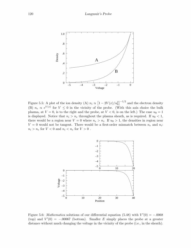
Figure 5.5: A plot of the ion density (A) ni ∝[

1 − 2V (x)/u20

]

−1/2and the electron density

(B) ne ∝ eV (x) for V ≤ 0 in the vicinity of the probe. (With this axis choice the bulkplasma, at V = 0, is to the right and the probe, at V < 0, is on the left.) The case u0 = 1is displayed. Notice that ni > ne throughout the plasma sheath, as is required. If u0 < 1,there would be a region near V = 0 where ne > ni. If u0 > 1, the densities in region nearV = 0 would not be tangent. There would be a first-order mismatch between ne and ni:ni > ne for V < 0 and ni < ne for V > 0 .

0 10 20 30 40

0

–1

–2

–3

–4

–5

Position

Vol

tage

0 10 20

0

–1

–2

–3

–4

–5

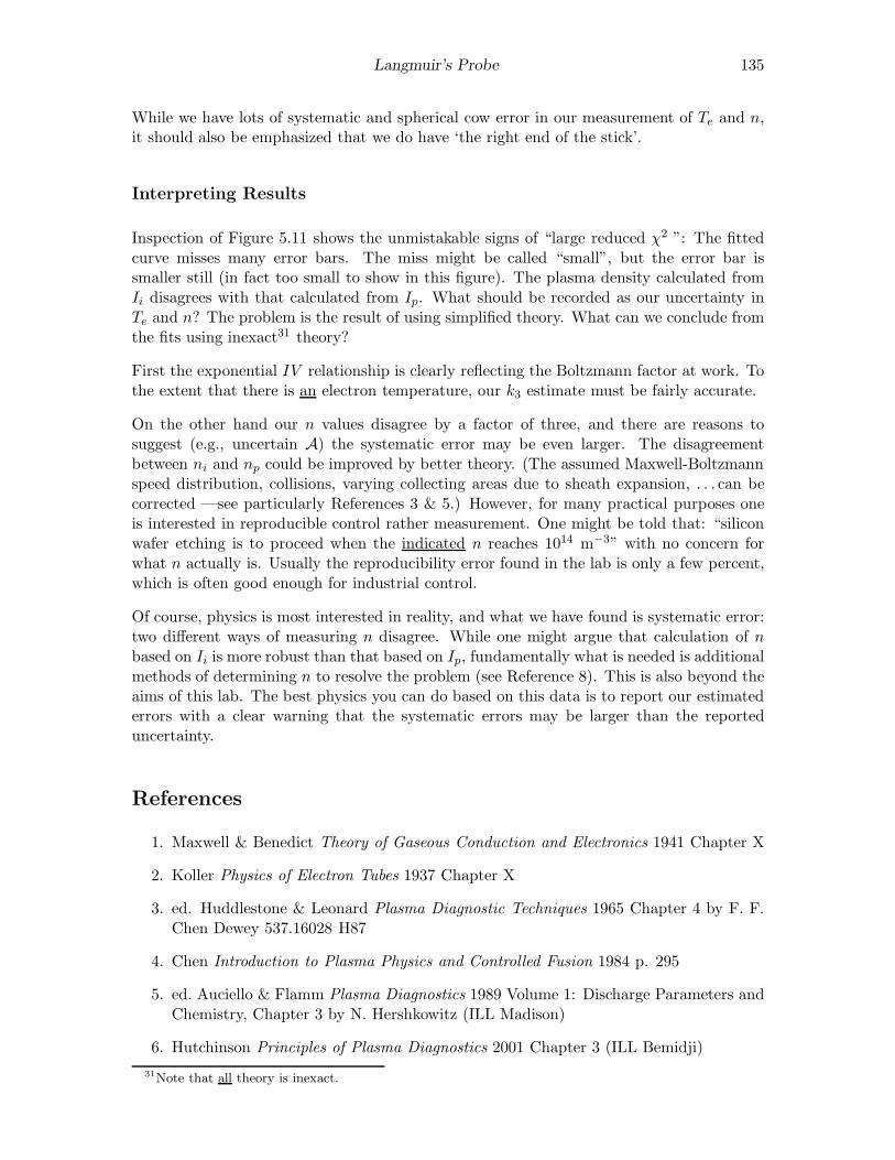
Figure 5.6: Mathematica solutions of our differential equation (5.48) with V ′(0) = −.0068(top) and V ′(0) = −.00067 (bottom). Smaller E simply places the probe at a greaterdistance without much changing the voltage in the vicinity of the probe (i.e., in the sheath).


larger region (“pre-sheath”, x ≪ 0), under conditions of near charge neutrality (ne ≈ ni),the ions traveled “downhill” a potential difference of:

V (−∞) − V (0) =K.E.

e=

12Miu

2B

e=

kTe

2e(5.50)

Thus, at x = 0, the plasma density has been depleted compared to that at x = −∞:

ni = ne = n0 = n∞e∆V/kTe = n∞e−1/2 (5.51)

The corresponding current density is:

J = en0u0 = en∞e−1/2uB ≈ .61 en∞

√

kTe

Mi(5.52)

Clearly this is an approximate argument. Other arguments can give lower (e.g., .40) con-stants. We adopt as our final equation (if only approximate: ±20%)

Ji ≈1

2en∞

√

kTe

Mi(5.53)

Region C

Plasma Potential, Vp

We have said that for V < Vp, the electron current to the probe is exponentially growingessentially because of the exponential form of the Maxwell-Boltzmann distribution. ForV > Vp, the electron current to the probe continues to grow, but only because of expandingcollecting area due to an expanding plasma sheath. The boundary between two cases isdefined by the point of maximum slope. The point where the slope is a maximum, of course,has the second derivative zero—an inflection point. Thus Vp is defined by I ′′(Vp) = 0. (Thisis called the Druyvesteyn criteria.)

In calculus you’ve learned how to apply a precise definition of derivative to find the deriva-tives of various functions, but how can you determine the second derivative from a set ofdata?

We begin with a qualitative treatment. If you have a set of equally spaced data points:xi = ih where i ∈ Z (i is an integer, h might have been called ∆x), then (f(xi+1)−f(xi))/h(the slope of a line through the points (xi, f(xi)) & (xi+1, f(xi+1)) ought to be somethinglike f ′(xi + h/2) (the derivative half way between xi & xi+1). Similarly, f ′(xi − h/2) ≈(f(xi) − f(xi−1))/h. Thus:

f ′′ ≈ f ′(xi + h/2) − f ′(xi − h/2)

h=

f(xi+1) + f(xi−1) − 2f(xi)

h2(5.54)

where we imagine f ′′ is evaluated half way between xi + h/2 & xi − h/2, that is, at xi.

More formally, theoretically f has a Taylor expansion:

f(xi + y) = f(xi) + f ′(xi)y +1

2f ′′(xi)y

2 +1

6f ′′′(xi)y

3 +1

24f ′′′′(xi)y

4 + · · · (5.55)


0 1 2

12

10

8

6

4

2

A

0 1 2

B

0 1 2

C

ƒ

ƒ´´

ƒ´

x x x

Figure 5.7: Numerical differentiation applied to the function f(x) = ex. f ′ and f ′′ have beenvertically offset by 2 and 4 respectively so that they do not coincide with f . (A) Here withh = .2, the numerically calculated f ′ and f ′′ (based on the shown data points) accuratelytrack the actual derivatives (shown as curves). (B) With random noise of magnitude ±.02added to the y values, the data points seem to accurately follow the function, but numericallycalculated f ′ and f ′′ increasingly diverge. See that numerical differentiation exacerbatesnoise. (C) Doubling the number of data points (with the same level of random noise as inB), makes the situation much worse. While the data points seem to follow f adequately, f ′

shows large deviations and f ′′ does not at all track the actual derivative.

So:

f(xi + h) = f(xi+1) = f(xi) + f ′(xi)h +1

2f ′′(xi)h

2 +1

6f ′′′(xi)h

3 +1

24f ′′′′(xi)h

4 + · · ·

f(xi − h) = f(xi−1) = f(xi) − f ′(xi)h +1

2f ′′(xi)h

2 − 1

6f ′′′(xi)h

3 +1

24f ′′′′(xi)h

4 + · · ·

f(xi + h) + f(xi − h) = 2f(xi) + f ′′(xi)h2 +

1

12f ′′′′(xi)h

4 + · · · (5.56)

with the result:

f(xi + h) + f(xi − h) − 2f(xi)

h2= f ′′(xi) +

1

12f ′′′′(xi)h

2 + · · · (5.57)

Thus if f ′′′′(xi)h2/f ′′(xi) ≪ 1 (which should follow for sufficiently small h), Equation 5.54

should provide a good approximation for f ′′(xi). While ever smaller h looks good mathe-matically, Figure 5.7 shows that too small h plus noise, is a problem.

Root Finding—Floating Potential, Vf & Plasma Potential, Vp

The floating potential is defined by I(Vf ) = 0. Of course, it is unlikely that any collecteddata point exactly has I = 0. Instead a sequence of points with I < 0 will be followed


by points with I > 0, with Vf lying somewhere between two measured points. We seek tointerpolate to find the best estimate for Vf .

We begin with the generic case, where we seek a root, i.e., the x value such that y(x) = 0.We start with two data points (x1, y1) and (x2, y2) with y1 < 0 and y2 > 0. The lineconnecting these two points has equation:

y =∆y

∆x(x − x1) + y1 =

y2 − y1

x2 − x1(x − x1) + y1 (5.58)

We seek the x value for which the corresponding y value is zero:

∆y

∆x(x − x1) + y1 = y = 0 (5.59)

x − x1 = −y1∆x

∆y(5.60)

x = x1 − y1∆x

∆y(5.61)

In the case of the floating potential (I(Vf ) = 0), our (xi, yi) are a sequence of voltages withmeasured currents: xi = Vi, yi = I(Vi), and we can apply the above formula to find thevoltage, Vf where the current is zero.

The same generic result can be used to estimate the plasma potential, where I ′′(Vp) = 0.Here xi = Vi, yi = I ′′(Vi). Just as in the floating voltage case, it is unlikely that anycollected data point exactly has I ′′ = 0. Instead a sequence of points with I ′′ > 0 will befollowed by points with I ′′ < 0, with Vp lying somewhere between two measured points.You will apply the generic interpolate formula to find the best estimate for Vp.

Electron Temperature, Te

If we combine Equation 5.36 for the ion current with Equation 5.35 for the electron current,we have an estimate for the total current through out Region C:

I = −1

2eA ni uB +

1

4eA ne

[

8kTe

πm

]1/2

exp

(

−e(Vp − V )

kTe

)

(5.62)

=1

2eA nuB

{

−1 +

[

2Mi

πm

]1/2

exp

(

−e(Vp − V )

kTe

)

}

(5.63)

= k1 + k2 exp ((V − Vp)/k3) (5.64)

Use of this equation is based on a long list of assumptions (e.g., constant collection area A,Maxwell-Boltzmann electron speed distribution, ni = ne = n. . . ). These assumptions arenot exactly true, so we do not expect this equation to be exactly satisfied: we are seeking asimplified model of reality not reality itself. By fitting this model equation to measured IVdata, we can estimate the parameters k1, k2, k3. Since k3 = kTe/e we can use it to estimatethe electron temperature. Similarly, k1 represents a measure of the ion current from which(once Te is known) ni can be calculated using Equation 5.36.

In order to start a non-linear fit as in Equation 5.64, we need initial estimates for theparameters ki. Measurement of Vf (where I = 0) and Equation 5.63, provide an estimate


for Te:

0 = I =1

2eA n uB

{

−1 +

[

2Mi

πm

]1/2

exp

(

e(Vf − Vp)

kTe

)

}

(5.65)

1 =

[

2Mi

πm

]1/2

exp

(

e(Vf − Vp)

kTe

)

(5.66)

0 =1

2ln

[

2Mi

πm

]

−(

e(Vp − Vf )

kTe

)

(5.67)

e

kTe(Vp − Vf ) =

1

2ln

[

2Mi

πm

]

(5.68)

kTe

e=

2(Vp − Vf )

ln[

2Mi

πm

] (5.69)

Notice that the unit for k3 = kTe/e is volts, so ek3 = kTe in units of J or, most simply,k3 = kTe in units eV17 (since eV=e×Volt). It is common practice in plasma physics toreport “the temperature” [meaning kT ] in eV.

The ion current k1 can be estimated from the “saturated current” in Region D, i.e., thenearly constant current a volt or so below Vf . (For future convenience, we name this“saturated current” in Region D, Ii.)

See that for V = Vp, I = k1 + k2. Since the ion current is “negligible” for most of region C,we can estimate k2 from the measured current near Vp. (For future convenience, we namethe current actually measured at the data point just below Vp, Ip.)

Plasma Number Density, n

Given kTe, we have several of measuring n:

A. measured Ii and Equation 5.36, and

B. measured Ip and Equation 5.32,

Additionally we could use the fit values of Ii or Ip (k1 or k2, in Equation 5.64). Thesemethods will give answers that differ by a factor of 5 or more! When different ways ofmeasuring the same thing give different results, “systematic error” is the name of theproblem. The source of this problem is our imperfect model of current flow in RegionC (all those inaccurate assumptions). In particular, both (A) and (B) are hindered by theassumption of a Maxwell-Boltzmann speed distribution. (In fact measurements in Region Care commonly used to measure18 that speed distribution.) Often fit parameters are preferredto individual data points (essentially because the fit averages over several data points), butthat is not the case here. Thus the method considered most accurate is (A), although it

17Recall: 1 eV = 1.6022 × 10−19 J is the energy an electron gains in going through a potential differenceof 1 V.

18For example, Langmuir probes have been used to measure the electron speed distribution in the plasmathat gives rise to aurora (northern lights). The results show a non-Maxwellian speed distribution: lots ofhigh-speed “suprathermal” electrons.


Table 5.1: R.C.A. 0A4-G Gas Triode Specifications

probe length 0.34 cmprobe diameter 0.08 cmtube volume (approx.) 40 cm3

peak cathode current 100 mADC cathode current 25 mAstarter anode drop (approx.) 60 Vanode drop (approx.) 70 Vminimum anode to cathode breakdown voltage(starter anode potential 0 volts) 225 V

could be improved19 to account for the slowly varying—rather than constant—ion currentin Region D. (That is, how precisely is the ion saturation current determined?) However,even with that ambiguity resolved, Equation 5.36 itself has expected variations of the orderof 20%. Mostly physicists just live with that level of accuracy, as improved measurementmethods (like microwave phase shifts due to the index of refraction of the plasma) are oftennot worth the effort.

Apparatus: 0A4-G Gas Triode Tube

Figure 5.8 displays the anatomy of a 0A4-G gas triode20. As shown in Figure 5.9, a dischargethrough the argon gas is controlled by a Keithley 2400 current source. Various cathodecurrents (Ic = −5,−10,−20,−40 mA) will produce various plasma densities. During tubeoperation, you should see the cathode glow expand as larger discharge currents are produced.Note also that the cathode voltage (Vc ∼ −60 V) varies just a bit, over this factor of 8increase in Ic. A glow discharge does not act like a resistor! A Keithley 2420 is used tosweep the probe voltage and simultaneously measure the probe current. Figure 5.10 showsrepresentative results. You should note that the cathode glow is not perfectly stable. It canjump in position for no obvious reason. If a jump occurs during a probe sweep, the resultingdata will look noisy (I ′′ randomly jumping in sign rather than smoothly going from I ′′ > 0to I ′′ < 0) and cannot be used. Figure 5.11 shows fits to the data between Vf and Vp. Theresulting reduced χ2 were of order 105: the measurement errors are much smaller than thedeviations between the reality and the model. While the model is “wrong”, it neverthelesssupplies a reasonable representation of the data. A fudge of the errors allows parametererror estimates to be extracted from the covariance matrix, but it’s hard to give meaningto the resulting error.

19This issue is addressed by Chen in report LTP-111 Chen206R.pdf listed as a web reference at the end ofthis document. Models of the Universe can usually be improved at a cost of greater complexity. Choosingan appropriate level of complexity is something of an art. Here we are using the simplest possible model.

20This tube is also called a cold cathode control tube. In its usual applications, what is here called theanode is called the starter anode and what is here called the Langmuir probe is called the anode.


Cathode

Anode

LangmuirProbe

Argon Gas

0A4−G

1

2

8

7

6

54

3

key

LangmuirProbe

Cathode Anode

Bottom View

Figure 5.8: The 0A4-G triode has a large cold cathode and two “anodes” surrounded by lowpressure argon gas. A glow discharge in the argon gas may be maintained by an approximate−60 V drop between the cathode (pin 2) and the “starter anode” (pin 7). The pin 5 anodemay then be used as a Langmuir probe in the resulting plasma. The figure shows an R.C.A.0A4G; A Sylvania 0A4G has the same components arranged differently.

1

2

8

7

6

54

3

key

2420voltagesource

2400current source

approx−60 V

Ic

Vc

V, I

red black

red

black

Figure 5.9: When the cathode is held at a voltage of Vc ≈ −60 V relative to the anode,the argon gas in the tube partially ionizes and a discharge is set up between the anode andcathode. The discharge current is controlled by a Keithley 2400 in current-source mode,e.g., Ic = −20 mA. The voltage V on the Langmuir probe is swept by the Keithley 2420, andthe current I is simultaneously measured. The resulting IV curve allows us to determinethe characteristics of the plasma. Note that the pinout shows the tube as viewed from thebottom.


–15 –10 –5 0 5

6.E–04

4.E–04

2.E–04

0

A

Voltage (V)

Cur

rent

(A

)

–14 –12 –10 –8 –6

4.E–06

3.E–06

2.E–06

1.E–06

0

B

Voltage (V)

Cur

rent

(A

)

Figure 5.10: The IV curves for the Langmuir probe in a 0A4G tube for Ic =−40,−20,−10,−5 mA. The plasma potential Vp is marked with a square; The floatingpotential Vf is marked with a circle. Since the ion current is so much smaller than theelectron current, blowing up the y scale by a factor of 200 is required to see it (see plot B).In this lab we are primarily concerned with Region C: between Vf and Vp.

–12 –10 –8 –6 –4

1.E–04

1.E–05

1.E–06

1.E–07

Voltage (V)

Cur

rent

(A

)

Figure 5.11: In Region C, between Vf and Vp, I > 0 so we can display it on a log scale.Assuming a constant ion current (k1), constant sheath area, and a Maxwell-Boltzmanndistribution of electron speed, we can fit: I(V ) = k1+k2∗exp((V −Vp)/k3). The horrendousreduced χ2 shows that these assumptions are not exact, nevertheless the fit does a reasonablejob of representing the data (say, ±10%)


Computer Data Collection

As part of this experiment you will write a computer program to control the experiment.Plagiarism Warning : like all lab work, this program is to be your own work! Programsstrikingly similar to previous programs will alarm the grader. I understand that program-ming may be new (and difficult) experience for you. Please consult with me as you writethe program, and test the program (with tube disconnected!) before attempting a finaldata-collecting run.

In the following I’m assuming the probe voltage V is stored in array v(i), probe currentI is stored in array a(i), and the second derivative of prove current I ′′ is stored in arrayapp(i). Your program will control all aspects of data collection. In particular it will:

0. Declare and define all variables.

1. Open (i.e., create integer nicknames—i.e., iunit—for) the enets gpib0 and gpb1.

2. Initialize the source-meters which must be told the maximum voltage and current tooccur during the experiment. For the 2420, you can limit V, I to 25. V and .005 A;For the 2400, limit V, I to 100. V and 0.1 A;

3. Display the status of all devices before starting data collection.

4. Open files:

(a) VI.dump.dat (intended for all V, I, I ′′ of probe, with comments (!) for cathodeIc, Vc)

(b) VI.fit.dat (intended for Region C: V, I, δI, I ′′ of probe, with comments forcathode Ic, Vc, calculated Vf , Vp, estimated Te, measured Ii, Ip, and the numberof data points. The data points in this file are for fitting Equation 5.64:

f(x) = k1 + k2 ∗ exp((x− k4)/k3) (5.70)

Note that k4=Vp is a constant, not an adjustable parameter.)

5. Tell the 2400 source-meter to source a cathode current, Ic = −20 mA

6. Let the system sleep for 60 seconds to approach thermal equilibrium.

7. Repeat the below data collection process six times. Since you will need just threerepeats for each Ic, this will probably produce more data than is needed. Howeversome data sets may be noisy because of unstable (moving, flickering) cathode glow.Noisy data will have multiple sign changes in calculated I ′′; Discard this data. Ifone run of this program fails to produce enough good data (three repeats), simplyrename the data files (to preserve the data produced in the initial run), and re-runthe program.

Do the following for four different Ic: 5, 10, 20 40 mA (e.g., acath=-.005*2**j forj=0,3). Thus there will be 4 × 6 voltage sweeps.

(a) Tell the 2400 source-meter to source a cathode current, Ic

(b) Let the system sleep for 10 seconds to approach thermal equilibrium.


(c) Tell the 2420 to perform a linear probe voltage sweep from Vmin to Vmax, includ-ing N data points (say, N = 100). In Figure 5.10, you can see that the choicemade was Vmin = −15. and Vmax = +5., but your choices will vary and mustbe determined by trial and error (see below). The aim is to find a range thatincludes from a few volts below Region C to a few volts above Region C for everycathode current Ic.

(d) Turn off the probe voltage.

(e) Repeat (a) thus obtaining up-to-date values for Ic, Vc

(f) Write a comment (‘!’) line to the file VI.dump.dat containing Ic, Vc from the2400.

(g) Write a line to the file VI.dump.dat containing the first probe (V, I) data point:v(1), a(1)

(h) Do for i=2,N-1 the following:

i. Calculate I ′′ and store the value in the ith spot of an array i.e.,app(i)=a(i+1)+a(i-1)-2*a(i).

ii. Write the probe data: V, I, I ′′, i.e., v(i), a(i), app(i), to the file VI.dump.dat

(i) Write a line to the file: VI.dump.dat containing the last (i=N) data point V, I.

(j) Find the data point just before Vf with code21 like:

do i=2,N-1

if(a(i)>0.and.a(i+1)>0)goto 100

enddo

100 ivf=i-1

if(ivf.lt.15) STOP

The final line halts the program if ivf< 15, as we need Region D data to find theion current, Ii. If the program STOPs, Vmin will need to be reduced to capturethis data, and the program re-run.

(k) Using Equation 5.61 and the data points at ivf and ivf+1, find Vf . Note: in thegeneral case Equation 5.61, we were seeking x such that y(x) = 0; Here we areseeking Vf which is defined as the voltage such that I(Vf ) = 0, so, for example,x1 →v(ivf), y1 →a(ivf), and x → Vf .

(l) Find the data point just before Vp with code22 like:

do i=ivf+1,N-2

if(app(i)>0.and.app(i+1)>0)goto 200

enddo

STOP

200 ivp=i-1

Note that the program is halted if the plasma potential has not been found beforewe run out of data. In that case Vmax will need to be increased to capture thisdata, and the program re-run.

21The check for two successive data points gone positive is done to avoid mistaking one point of noise forVf .

22The check for two successive data points with I′′

< 0 is done to avoid mistaking one point of noise forVp


(m) Using Equation 5.61 and the data points at ivp and ivp+1, find Vp. Note Vp

is defined as the voltage such that I ′′(Vp) = 0, so, for example, x1 →v(ivp),y1 →app(ivp) , and x → Vp.

(n) Write comment lines to the file: VI.fit.dat recording:

i. Ic, Vc, Vf , Vp (also print this to the screen, so you can monitor data collec-tion)

ii. ’!set k1= ’,a(ivf-15),’ k2= ’,a(ivp),’ k3= ’, 0.18615*(Vp − Vf )The aim here is to record basic plasma parameters (which are also neededas an initial guess in the fit to Equation 5.70) in a format that allows easycopy and paste into plot and fit. k1 is the measured ion current Ii; k2 isthe measured current at Vp (denoted Ip); k3 is an estimate for kTe/e, theelectron temperature in eV.Notes: The estimate for k3 is based on Equation 5.69 where 0.18615 =2/ ln(2Mi/πm). We are assuming that ivf-15 is far enough below Vf (i.e.,in Region D) that Ii = a(ivf− 15). You should check (after the fact) thatthis is the case, i.e., Vf − v(ivf− 15) ≫ k3. If this condition is not met,simply use a larger offset than 15 and re-run the program.

iii. ’!set k4= ’, Vp, ’ npoint= ’, ivp-ivf

k4 is the (not adjusted) plasma potential, Vp, whereas k1-k3 are varied fromthe above initial guesses to get the best fit to Equation 5.70 in Region C.

(o) For i=ivf+1,ivp write the probe data V, I, δI, I ′′ to the file VI.fit.dat withone V, I, δI, I ′′ data ‘point’ per line.

8. Turn off the output of the 2400.

9. Close all files.

Data Analysis

If all has gone well you have three good data sets for four different Ic, something like 1000data points. We could spend the next semester analyzing this data! Instead I suggest belowa simplified analysis scheme.

Start by making a composite plot similar to Figure 5.10A showing one IV curve for each ofthe four Ic. For these plots, choose Vmin & Vmax so that all behaviors (Regions A–D) aredisplayed. Make a similar plot showing three IV curves for one of the four Ic. The aim hereis to test for reproducibility; because of time limitations we’ll just check the reproducibilityof this one selected Ic. (I’ll call this selected Ic data set I∗c .) These six data sets (one IVcurve is on both plots) will be analyzed in greater detail. In order to properly fit the data,you will want to have more than 15 data points in the region between Vf and Vp (this mayrequire reducing the range Vmin through Vmax for the probe voltage sweep so it focuses juston Region C: say from about 4 V negative of the lowest Vf to 2 V positive of the highestVp and then re-taking the data). Additionally you should find that all six data sets haveapproximately the same number of data points.

Electron Temperature in eV: k3Fit Equation 5.70 to the six data sets. Note that the file itself contains the required initialguesses for adjusted parameters k1-k3 and the fixed value for k4. Expect to see large


reduced χ2 which signals a too-simple model. No definite meaning can be attached to error

estimates from such poor fits, nevertheless some sort of nonsense needs to be reported.On page 16 we explored options for dealing with such ‘unusual’ fits. Option #5: ‘In direcircumstances’ you can use fudge command in fit to change your errors so that a reducedχ2 near one will be obtained. A re-fit with these enlarged errors then gives a new covariancematrice from which an estimate of parameter errors can be determined. Parameter valueswithin the range allowed by these errors would produce as good (or bad) a fit to the dataas the ‘best’ values. As the name suggests fudge is not exactly legitimate23 , neverthelessit is what Linfit has been silently doing all these years. Option #4: ‘Bootstrap’ the data:repeatedly fit subsets of the data and see how the resulting fit parameters vary with themultiple fits. This is essentially a way to repeat the experiment without taking new data.The fit command boots will report the results of nboot (default: 25) re-fits to subsets ofyour data along with the standard deviation of the fit parameters. Using either option, weare particularly interested in the some estimate of error in fit value of k3: use the squareroot of the appropriate diagonal element of the covariance matrice of a fudged fit or thereported standard deviation of k3 from a bootstrap.

For I∗c , compare the two errors for k3: σ (standard deviation of 3 fit values of k3) and thatfrom the fudged covariance matrix. Are they in the same ballpark (say, within a factor oftwo)?

Calculate the electron temperature of the plasma both in eV and K. Comment on therelationship (if any) between Te and Ic.

Plasma Number Density: nWe are interested in two sorts of ‘error’ in the plasma density n: reproducibility and anestimate of ‘systematic’ error. In the first case we’re asking: “given the same Ic is applied,how much do conditions in the plasma vary?” In the second case we interested in what theactual value of n is. We can estimate this systematic error by measuring n by two differentmethods:24 n calculated using Ii (Method A: let’s call this ni) and n calculated using Ip

(Method B: let’s call this np). Let’s be clear here: ni, np, ne, n are all supposed to be thesame thing: the number of electrons (or ions) per m3 in the plasma. So

np

ni=

−Ip/Ii√

2Mi/πm(5.71)

should be one; but it won’t be: systematic error is present!

In your lab notebook record these results in tables similar that shown in Table 5.225. (Forthis example, I selected I∗c = 20 mA.) Note particularly to record exactly the proper numberof significant figures in these tables! You should also copy & paste each full fit report into along concatenated file and include the resulting file in your notebook. As previously noted,the reduced χ2 for these fits is likely to be “horrendous”. Pick out your highest reduced χ2

fit, and plot the fitted function along with the data points on semi-log paper. (The resultsshould look similar to Figure 5.11, but with just one data set.) Do the same for the bestfit.

23for further discussion see: http://www.physics.csbsju.edu/stats/WAPP2 fit.html24See page 124; we are discussing here only methods A and B; methods using the fit parameters k1 and

k2 would be additional options.25The spreadsheet gnumeric may be of use.


Table 5.2: Simplified data table for reporting Langmuir Probe results.

k3 Ic k3 fit σ(V) (mA) (V) error

40

20

105

Ii Ic median σ % error ni % error(A) (mA) Ii in Ii (m−3) in ni

40

20

10

5

Ip Ic median σ % error np/ni

(A) (mA) Ip in Ip

40

20

10

5

Calculate26 n for each Ic based on the median Ii. Comment on the relationship (if any)between n and Ic. Make a power-law fit and log-log plot of the data27

Derive Equation 5.71. Calculate the np/ni and see that n has systematic error, i.e., ncalculated from Ip will be several times larger than the value of n calculated from Ii. Thisproves that there are problems with our simple theory.

Miscellaneous Calculations: ‘Lawson Product’ nτ , λD, fp

In 1957 J. D. Lawson determined that power generation from thermonuclear fusion requiredtemperature, plasma density n and the plasma confinement time τ to meet certain criteria:a temperature of at least 104 eV with the product: nτ > 1021 m−3 · s. We can estimate τbecause we know that our plasma is moving toward any surface at the Bohm velocity uB .Given that typically the plasma is within about 1 cm of a wall, find how long it remainsconfined, and calculate the “Lawson product” nτ for the I∗c plasma. (It is possible todirectly measure the plasma confinement time by using a scope to time the decay of theplasma when the glow discharge is suddenly turned off.)

Calculate the Debye length (λD, Eq. 5.14) and the plasma frequency (fp, Eq. 5.1) for I∗c .Compare λD to the diameter of the Langmuir probe. Will the sheath substantially expandthe collecting area A? According to Koller (p. 140, reporting the results of Compton &Langmuir28) the mean free path of an electron in a 1 torr argon gas is 0.45 mm. Compare

26http://www.physics.csbsju.edu/cgi-bin/twk/plasma.html can do this in one click.27I’d use WAPP+ : http://www.physics.csbsju.edu/stats/WAPP2.html.28Rev. Mod. Phys. 2 (1930) 208


your λD to this electron mean free path.

Report Checklist

1. Write an introductory paragraph describing the basic physics behind this experiment.For example, why does the Langmuir probe current increase exponentially with probevoltage? Why is it that probe currents allow the calculation of plasma density? (Thismanual has many pages on these topics; your job is condense this into a few sentencesand no equations.)

2. Computer program: Print out a copy of your program and tape it into your labnotebook.

3. Plots:

(a) Similar to Figure 5.10A showing one IV curve for each of the four Ic.

(b) Similar to Figure 5.10A but showing three IV curves for I∗c .

(c) Two plots similar to Figure 5.11, showing the Region C fit to the data. (Theseplots are to display the best and worst reduced χ2; Record the reduced χ2 oneach plot.)

(d) Power law fit and log-log plot of four (Ic, n) data points.

4. Tabulated results from six fits for k3 (Te) at four different cathode currents includingfudged or bootstrapped results for δk3 and the standard deviation of three k3 for I∗c .You should copy & paste each full fit report into a long concatenated file. Print thatfile and tape it into your notebook. Record the identifying letter on your tube.

5. Tabulated results for measured Ii and Ip at four different cathode currents includingreproducibility errors estimated from the standard deviation.

6. Calculations (self-document spreadsheet or show sample calculations):

(a) kTe in units if eV for four Ic with estimates for errors.

(b) Te in units of K for four Ic.

(c) n calculated from median Ii and k3 for four Ic (with and estimate of reproducibil-ity error)

(d) np/ni calculated from median Ii and Ip (which provides an estimate of systematicerror)

(e) λD

(f) fp

(g) Lawson product at I∗c

7. Derivation of np/ni (Eq. 5.71).

8. Answers to the questions posed in the Data Analysis section:

(a) Are they in the same ballpark?

(b) Comment on the relationship (if any) between Te and Ic.


(c) Comment on the relationship (if any) between n and Ic.

(d) Will the sheath substantially expand the collecting area A?

(e) Compare your λD to this electron mean free path.

9. Discussion of errors:

(a) Two methods were used to find “errors” in the electron temperature, Te: (A)fudged/bootstrap error from a fit and (B) σ from lack of reproducibility. Whatis the meaning and significance of fudged/bootstrap error? What is the meaningand significance of reproducibility error? How would you respond to the question:“What is the error in Te?” (Note a few sentences are required, not a number!)

(b) Two methods were used to find the plasma number density, n: methods basedon Ii and Ip. What is the meaning and significance of the fact that two differentways of measuring n produced different results. How would you respond to thequestion: “What is n?” (Note a few sentences are required, not a number!)

(c) Consider any one of the basic plasma parameters (n, Te, Vf , Vp) measured in thislab. Report any evidence that there is systematic error in the parameter. Reportyour best guess for the total error (systematic and random) in the parameter.Report how this error could be reduced.

Comment: Uncertainty

Area: Systemtic Error

Both methods of calculating plasma density (ni and np) used the probe area A, which en-tered as an overall factor. The probe area was calculated based on the probe geometry datalisted in Table 5.1 which was supplied by reference #9 with no uncertainties. Clearly if theactual probe geometry differs from that in Table 5.1 there will be a systematic error in bothmethods of calculating n. If I guess the uncertainty in length and diameter measurementsbased on the number of supplied sigfigs, I find a 6% uncertainty in A. In 2008 a Sylvania0A4G tube was destroyed, and I took the opportunity to measure the the probe. The re-sults29 were quite different from those reported in Table 5.1: A was about 20% larger forthis Sylvania tube then for the RCA tube of reference #9. (The Sylvania/GE 0A4G alsolooks different from the RCA 0A4G.)

There is an additional significant problem: because the plasma sheath extends several λD

beyond the physical probe, there will be particle collection beyond the surface area of theprobe—the effective area is larger than the geometric surface area; we have made a SphericalCow by the simple assumption of A = πdℓ. A glace at Fig. 5.6 on page 120, shows thatthe plasma sheath extends about 10 × λD for ∆V ∼ 5 × kTe/e, which amounts to a largecorrection to probe diameter. Since the plasma sheath for ions30 in Region D has no reasonto be identical to the plasma sheath for electrons at the plasma potential, the effective Ain the two methods is probably not the same, and hence A does not really cancel out inderiving Eq. 5.71.

29diameter= 0.025”, length= .2”, the surrounding metal can is about 2 cm×3 cm.30For example, the mean free path for an electron is much larger than the mean free path for an ion

(approximately 4√

2×).


While we have lots of systematic and spherical cow error in our measurement of Te and n,it should also be emphasized that we do have ‘the right end of the stick’.

Interpreting Results

Inspection of Figure 5.11 shows the unmistakable signs of “large reduced χ2 ”: The fittedcurve misses many error bars. The miss might be called “small”, but the error bar issmaller still (in fact too small to show in this figure). The plasma density calculated fromIi disagrees with that calculated from Ip. What should be recorded as our uncertainty inTe and n? The problem is the result of using simplified theory. What can we conclude fromthe fits using inexact31 theory?

First the exponential IV relationship is clearly reflecting the Boltzmann factor at work. Tothe extent that there is an electron temperature, our k3 estimate must be fairly accurate.

On the other hand our n values disagree by a factor of three, and there are reasons tosuggest (e.g., uncertain A) the systematic error may be even larger. The disagreementbetween ni and np could be improved by better theory. (The assumed Maxwell-Boltzmannspeed distribution, collisions, varying collecting areas due to sheath expansion, . . . can becorrected —see particularly References 3 & 5.) However, for many practical purposes oneis interested in reproducible control rather measurement. One might be told that: “siliconwafer etching is to proceed when the indicated n reaches 1014 m−3” with no concern forwhat n actually is. Usually the reproducibility error found in the lab is only a few percent,which is often good enough for industrial control.

Of course, physics is most interested in reality, and what we have found is systematic error:two different ways of measuring n disagree. While one might argue that calculation of nbased on Ii is more robust than that based on Ip, fundamentally what is needed is additionalmethods of determining n to resolve the problem (see Reference 8). This is also beyond theaims of this lab. The best physics you can do based on this data is to report our estimatederrors with a clear warning that the systematic errors may be larger than the reporteduncertainty.

References

1. Maxwell & Benedict Theory of Gaseous Conduction and Electronics 1941 Chapter X

2. Koller Physics of Electron Tubes 1937 Chapter X

3. ed. Huddlestone & Leonard Plasma Diagnostic Techniques 1965 Chapter 4 by F. F.Chen Dewey 537.16028 H87

4. Chen Introduction to Plasma Physics and Controlled Fusion 1984 p. 295

5. ed. Auciello & Flamm Plasma Diagnostics 1989 Volume 1: Discharge Parameters andChemistry, Chapter 3 by N. Hershkowitz (ILL Madison)

6. Hutchinson Principles of Plasma Diagnostics 2001 Chapter 3 (ILL Bemidji)

31Note that all theory is inexact.


7. http://www.physics.uiowa.edu/~fskiff/Physics_132/Lab%20Manual/B4Langmuir.PDF

8. http://www.ee.ucla.edu/~ffchen/Publs/Chen206R.pdf

9. I. Alexeff, J. T. Pytlinski, and N. L. Oleson Am. J. Phys. 45 (1977) 860–866, alsosee Am. J. Phys. 45 (1977) 1196–1199, Am. J. Phys. 46 (1978) 1276–1278, Am. J.Phys. 52 (1984) 753–754

Documents

5: Langmuir’s Probe - College of Saint Benedict and Saint … · 2008-05-23 · Sunlight powers the creation of new ions in the ionosphere, ... In photoionization, electrons receive