Development of the ResidentialLoad Factor Method for Heatingand Cooling Load Calculations

Charles S. Barnaby Jeffrey D. Spitler, PhD, PEMember ASHRAE Fellow ASHRAE

4768 (RP-1199)

ABSTRACT

The recent ASHRAE project, “Updating the ASHRAE/ACCA Residential Heating and Cooling Load CalculationProcedures and Data” (RP-1199), developed two new resi-dential loads calculation procedures: residential heat balance(RHB), a detailed heat balance method that requires computerimplementation, and residential load factor (RLF), a simpli-fied procedure that is hand tractable and suitable for spread-sheet implementation. This paper describes RLF and itsdevelopment. The form of RLF resembles prior methods.However, the sensible cooling load procedure was derivedusing linear regression to find relationships between designconditions, building characteristics, and peak cooling loadpredicted by RHB. This eliminated the need for semi-empiricaladjustments, such as averaging, that have been used in thedevelopment of other methods. Results comparing RLF to RHBare presented. The RLF heating load calculation is alsodescribed; it uses the traditional UA∆T formulation except forimprovements to procedures for infiltration leakage rate andground (slab and basement) losses.

INTRODUCTION

The research project, “Updating the ASHRAE/ACCAResidential Heating and Cooling Load Calculation Proce-dures and Data” (RP-1199), had two primary products. First,a new fundamental residential heating and cooling load calcu-lation method was developed and tested. This procedure,called the residential heat balance (RHB) method, is based onheat balance first principles as described by Pedersen et al.(1997, 1998) and ASHRAE (2001). RHB is documented byBarnaby et al. (2005). It uses a computationally intensive 24-hour design-day simulation that is practical only when imple-

mented in software. Because of its fundamental approach,RHB can be applied with few restrictions to arbitrarilycomplex residential buildings, including those with largefenestration areas, novel construction features, or having non-summer peaks.

The ResHB computer program, developed as part of RP-1199, implements the RHB method as described in Barnaby etal. (2004). ResHB is a batch-driven FORTRAN-90 applica-tion derived from the ASHRAE Loads Toolkit (Pedersen et al.2001) that operates on Windows-based PCs. Several keyResHB features are noted here. First, ResHB models roomtemperature swing: in addition to the standard fixed-setpointcapability, ResHB can find the sensible cooling extraction ratethat results in a specified temperature swing above the ther-mostat setpoint. Second, ResHB incorporates the updatedmodels identified in RP-1199 as appropriate for residentialloads calculation. Third, ResHB is multi-room and multi-zone, allowing application to real buildings as well as simpletest cases. Finally, ResHB can model typical residentialmaster-slave control, where a thermostat in one room controlsthe cooling delivery in another, with resulting imperfecttemperature control in the slave room.

The second product of RP-1199 is a simpler procedure,designated “residential load factor” (RLF) method. RLF istractable by hand or can be straightforwardly implementedusing spreadsheet software. This simplification is achieved atthe expense of generality—RLF is applicable only to conven-tionally constructed residences with typical space-condition-ing requirements. The procedures and data required to useRLF are presented in the “Residential Heating and CoolingLoads Calculation” chapter of the 2005 ASHRAE Handbook—Fundamentals (ASHRAE 2005).

©2005 ASHRAE. 291

Charles S. Barnaby is vice president of research at Wrightsoft Corporation, Lexington, Mass. Jeffrey D. Spitler is CM Leonard Professorin the School of Mechanical and Aerospace Engineering, Oklahoma State University, Stillwater, Okla.

This paper discusses the design of RLF and documentsthe methodology used in its development. Some testing resultsare also presented. While RLF includes both cooling and heat-ing load procedures, the heating calculations rely on the tradi-tional UA∆T model that has proven satisfactory for decades.Improvements have been introduced in relation infiltrationleakage rate and to ground heat loss.

The RLF cooling procedure resembles and builds uponprior methods but was developed using a linear regressionapproach that avoids some semi-empirical derivations used inthe past. Prior methods have been published by the Air-Condi-tioning Contractors of America (ACCA), including the widelyused Manual J, seventh edition (ACCA 1986) and Manual J,eighth edition (ACCA 2003). The 1989-2001 editions of theASHRAE Handbook—Fundamentals included a methodbased on 342-RP (McQuiston 1984). Canadian StandardCAN/CSA-F280-M90 (HRAI 1996; CSA 1990) specifies acooling method also based on 342-RP and a heating procedurethat includes enhanced ground loss calculations.

RLF COOLING LOAD CALCULATION

The RLF cooling load calculation is based on the idea ofindependent load components, as are prior simplified meth-ods. The load contributions from various sources are sepa-rately evaluated and then summed. The following sectionssummarize the method, showing both sensible and latentcomponents as applicable. Later sections document the deri-vation of the component models and coefficients.

In RLF, surfaces have associated load factors (LFs) orload contribution per unit area. These are designated CFs forcooling and HFs for heating. For the most part, HF values aresimply U∆T. CF values depend on surface construction,climate, and, in some cases, surface orientation, solar absorp-tance, or other characteristics. Each unique LF needs to beevaluated once for a given set of site and construction condi-tions and then is applied repeatedly to building elements of thesame type. This two-step process is convenient for hand orspreadsheet application. Note that LFs are the functionalequivalent of Manual J’s heat transfer multipliers (HTMs) butare derived differently and in general do not have the samevalues.

Total Cooling Load

(1)

(2)

whereqs = sensible cooling load, W (Btu/h)ql = latent cooling load, W (Btu/h)Ai = area of ith surface, m2 (ft2)CFi = cooling factor of ith surface, W/m2 (Btu/h⋅ft2)

Opaque Surfaces

The cooling load per unit area of opaque walls, ceilings,and non-slab floors is calculated as follows:

(3)

whereCFopq = opaque surface cooling factor, W/m2

(Btu/h⋅ft2)U = construction U-factor, W/m2⋅K

(Btu/h⋅ft2⋅°F)∆T = design dry-bulb temperature difference

(outdoor – indoor), K (°F)DR = daily range of outdoor dry-bulb

temperature, K (°F)OFt, OFb, OFr = coefficients from Table 1

Slab floors produce a slight reduction in cooling load, asfollows:

(4a)

(4b)

whereCFslab = slab cooling factor, W/m2 (Btu/h⋅ft2)hsrf = effective surface conductance, including resistance

of slab-covering material such as carpet, W/m2⋅K (Btu/h⋅ft2⋅°F); 1/(Rcvr + 0.12) W/m2⋅K or 1/(Rcvr + 0.68) Btu/h⋅ft2⋅°F

qs Ai∑ CFi⋅ qvi ,s qig ,s+ +=

ql qvi ,l qig,l+=

CFopq U OFt T∆⋅ OFb OFr+ + DR⋅( )⋅=

CFslab 1.6 1.4– hsrf⋅=

CFslab 0.51 2.5 hsrf⋅–=

Table 1. Opaque Surface Coefficients

Surface Type Construction OFt OFb OFr

Ceiling or knee wall adjacent to vented attic Wood frame 0.62 14.1 ⋅ ∝roof – 4.3(25.4 · ∝roof – 7.7)

–0.23

Ceiling/roof assembly Wood frame 1 39 ⋅ ∝roof – 6.8(70.2 ⋅ ∝roof – 12.2)

–0.42

Wall Wood frame 1 7.9 (14.2) –0.34

Floor over ambient Wood frame 1 0 –0.10

Floor over crawlspace Wood frame 0.32 0 –0.46αroof = roof solar absorptance

292 ASHRAE Transactions: Research

Fenestration

Fenestration cooling factors are calculated as follows:

(5)

where

CFfen = fenestration cooling factor, W/m2 (Btu/h⋅ft2)

U = fenestration NFRC heating U-factor, W/m2⋅K(Btu/h⋅ft2⋅°F)

DR = daily range of outdoor dry-bulb temperature, K (°F)

∆T = cooling design temperature difference, K (°F)

FFs = load factor (see Table 2)

PXI = peak exterior irradiance, including shading modifications (see below), W/m2 (Btu/h⋅ft2)

SHGC = fenestration rated or estimated NFRC solar heat gain coefficient

IAC = interior shading attenuation coefficient

Peak exterior irradiance (PXI) is the hourly maximumsolar gain incident on the surface.

(6)

(7)

where

PXI = peak exterior irradiance for exposure, W/m2 (Btu/h⋅ft2)

Et, Ed, ED = peak total, diffuse, and direct irradiance for exposure, W/m2 (Btu/h⋅ft2)

Tx = transmission of exterior attachment (see Table 4)

Fshd = fraction of fenestration shaded by permanent overhangs, fins, or environmental obstacles

For horizontal or vertical surfaces, irradiance values canbe obtained from Table 3 for primary exposures or Algorithm1 for any exposure. Skylights with slope less than 30° fromhorizontal should be treated as horizontal. Steeper slopes,other than vertical, are not supported by the RLF method.

Algorithm 1. Exterior irradianceHorizontal surfaces

Vertical surfaces

where

Et, Ed, ED = peak hourly total, diffuse, and direct irradiance, W/m2 (multiply by 0.317 to convert to Btu/h·ft2)

L = site latitude, °N or °S

= exposure (surface azimuth), ° from south (–180 to +180)

The shaded fraction, Fshd, can be taken as 0 for fenestra-tion in full sun and 1 for any fenestration that is shaded by adja-cent structures or other obstacles during peak hours. Fshd forsimple overhang configurations can be calculated as follows(more complex configurations should be analyzed with theRHB method):

(8)

where

SLF = shade line factor from Table 5

Doh = depth of overhang (from plane of fenestration), m (ft)

Xoh = vertical distance from top of fenestration to overhang, m (ft)

H = height of fenestration, m (ft)

The shade line factor (SLF) is the ratio of the distancea shadow falls beneath the edge of an overhang to the width ofthe overhang (Table 5). Therefore, the shade line equals theSLF times the overhang depth. The tabulated values are theaverage of the shade line values for 5 h of maximum solarintensity on August 1 on each wall exposure shown. Windowsfacing north, northeast, and northwest are not effectivelyprotected by roof overhangs; in most cases, they should not beconsidered shaded.

Table 2. Fenestration Coefficients

Exposure FFs

N 0.17

NE 0.09

E 0.17

SE 0.25

S 0.45

SW 0.54

W 0.48

NW 0.34

Horiz 0.66

CFfen U T∆ 0.49– DR⋅( )⋅ FFs+ PXI SHGC IAC⋅ ⋅ ⋅=

PXI TxEt= (unshaded)

PXI Tx Ed 1 Fshd–( )ED+( )= (shaded)

Et 970 6.2L 0.16L2

–+= Ed MIN Et 124,( )=

ED Et Ed–=

Ψ ψ180---------= (normalized exposure)

Et 462.2 1625Ψ 6183Ψ3

– 3869Ψ4

32.38ΨL+ + +=

0.3237+ ΨL2

12.56L– 0.8959L2

–1.040L

2

Ψ 1+-------------------+

Ed MIN Et 392.1, 138.6Ψ– 2.107ΨL121 L4

Ψ 1+-----------------–+⎝ ⎠

⎛ ⎞=

ED Et Ed–=

ψ

Fshd MIN 1,MAX 0,SLF Doh⋅ Xoh–

H---------------------------------------

⎝ ⎠⎛ ⎞

⎝ ⎠⎛ ⎞=

ASHRAE Transactions: Research 293

Ventilation and Infiltration

Infiltration airflow is calculated as follows:

(9)

Qinf = infiltration airflow rate, L/s (cfm)AL = building effective leakage area (including flue) at

4 Pa assuming CD = 1, cm2 (in.2)I0 – I2 = coefficients, as follows:

H = building average stack height, m (ft) (approximately 2.5 m [8 ft] per story)

∆T = indoor-outdoor temperature difference, K (°F)

AL,flue = flue effective leakage area at 4 Pa assuming CD = 1, cm2 (in.2)

The ventilation airflow rate is determined according to theinstalled or planned ventilation equipment that is expected tobe operating at design conditions. Generally, intermittently

Table 3. Exterior Irradiance (W/m2)

Exp

Latitude (°N or °S)

20 25 30 35 40 45 50 55 60

N ED 132 117 106 101 103 110 124 145 172

Ed 136 122 109 98 88 79 70 63 55

Et 269 238 215 199 190 189 194 207 227

NE/NW ED 541 532 522 511 501 490 480 470 461

Ed 163 154 147 140 135 130 126 123 120

Et 704 686 668 652 636 621 606 593 580

E/W ED 627 640 650 657 662 663 662 659 653

Ed 173 169 166 163 162 161 161 161 162

Et 800 809 816 821 824 825 823 820 815

SE/SW ED 334 380 422 460 494 525 553 577 598

Ed 174 173 174 175 177 180 183 187 191

Et 508 553 595 635 672 705 736 764 788

S ED 0 65 146 223 297 368 436 501 563

Ed 149 171 175 180 186 192 198 205 212

Et 149 236 321 403 482 559 634 705 774

Hor ED 906 901 888 867 838 801 756 703 642

Ed 124 124 124 124 124 124 124 124 124

Et 1030 1025 1012 991 962 925 880 827 766Note: multiply value by 0.317 to convert to Btu/h⋅ft2

Table 4. Exterior Attachment Transmission

Attachment Tx

Exterior insect screen 0.6

Shade screen Manufacturer SC value, typically 0.4 to 0.6Note: see Brunger et al. 1999 re: insect screens

Qinf

AL

1000------------ I0 H+ T∆ I1 I2+

AL ,flue

AL

----------------⋅⎝ ⎠⎛ ⎞⋅ ⋅⋅=

CoolingWindspeed—

3.4 m/s (7.5 mph)

HeatingWindspeed—

6.7 m/s (15 mph)

I0 25 (343) 51 (698)

I1 0.38 (.88) 0.35 (.81)

I2 0.12 (.28) 0.23 (.53)

294 ASHRAE Transactions: Research

operated exhaust fans are not included. Overall supply andexhaust flow rates are determined and divided into “balanced”and “unbalanced” components and combined with infiltration.

(10)

(11)

(12)

whereQbal = balanced ventilation airflow rate, L/s (cfm)Qsup = total ventilation supply airflow rate, L/s (cfm)Qexh = total ventilation exhaust airflow rate (including any

combustion air requirements), L/s (cfm)Qunbal = unbalanced airflow rate, L/s (cfm)Qvi = combined infiltration/ventilation flow rate (not

including balanced component), L/s (cfm)Note that unbalanced duct leakage can produce additional

pressurization or depressurization. This effect is included indistribution losses, discussed below.

The cooling (or heating) load due to ventilation andinfiltration is calculated as follows, taking into account theeffects of heat/energy recovery ventilation (HRV/ERV) equip-ment:

(13)

(14)

(15)

(16)

whereqvi,s = sensible ventilation/infiltration load, W (Btu/h)Cs = air sensible heat factor, 1.23 W/(L/s)⋅K

(1.1 Btu/h⋅cfm⋅°F) at sea levelεs = HRV/ERV sensible effectivenessQbal,hr = balanced ventilation flow rate supplied via HRV/

ERV equipment, L/s (cfm)Qbal,oth = other balanced ventilation supply airflow rate, L/s

(cfm)∆T = indoor-outdoor temperature difference, K (°F)

qvi,l = latent ventilation/infiltration load, W (Btu/h)Cl = air latent heat factor, 3010 W/(L/s) (4840 Btu/h-cfm)

at sea level∆W = indoor-outdoor humidity ratio differenceqvi,t = total ventilation/infiltration load, W (Btu/h)Ct = air total heat factor, 1.2 W/(L/s)⋅(kJ/kg)

(4.5 Btu/h⋅cfm⋅(Btu/lb)) at sea levelεt = HRV/ERV total effectiveness∆h = indoor-outdoor enthalpy difference, kJ/kg (Btu/lb)

Internal Gain

The contributions of internal gains to peak sensible andlatent loads are:

(17)

(18)

whereqig,s = sensible cooling load due to internal gains, W (Btu/h)qig,l = latent cooling load due to internal gains, W (Btu/h)Gx = coefficients, as follows:

Acf = conditioned floor area of building, m2 (ft2)Noc = number of occupants; if not known, estimate as

(number of bedrooms + 1)

Distribution Losses

The allowance for distribution losses is calculated asfollows:

(19)

whereqdl = distribution loss, W (Btu/h)Fdl = distribution loss factor, from Table 6qs = building sensible load, W (Btu/h)

Table 5. Shade Line Factors (SLF)

Window Exposure

Latitude, °N

24 32 36 40 44 48 52

East 0.8 0.8 0.8 0.8 0.8 0.8 0.8

SE 1.8 1.6 1.4 1.3 1.1 1.0 0.9

South 9.2 5.0 3.4 2.6 2.1 1.8 1.5

SW 1.8 1.6 1.4 1.3 1.1 1.0 0.9

West 0.8 0.8 0.8 0.8 0.8 0.8 0.8Note: Shadow length below the overhang equals the shade line factor times the overhang depth.

Qbal MIN Qsup,Qexh( )=

Qunbal MAX Qsup,Qexh( ) Qbal–=

Qvi MAX Qunbal,Qinf 0.5 Qunbal⋅+( )=

qvi ,s Cs Qvi 1 εs–( )+ Qbal ,hr⋅ Qbal,oth+( ) T∆⋅ ⋅=

qvi ,l Cl Qvi Qbal ,oth+( ) W∆⋅ ⋅= (no HRV/ERV)

qvi ,t Ct Qvi 1 εt–( )+ Qbal ,hr⋅ Qbal,oth+( ) h∆⋅ ⋅=

qvi ,l qvi ,t qvi ,s–=

Sensible Latent

G0 136 (464) 20 (68)

Gcf 2.2 (0.7) 0.22 (0.07)

Goc 22 (75) 12 (41)

qig,s G0,s Gcf ,s+ Acf⋅ Goc,s+ Noc⋅=

qig ,l G0,l Gcf ,l+ Acf⋅ Goc ,l+ Noc⋅=

qdl Fdl qs⋅=

ASHRAE Transactions: Research 295

DEVELOPMENT OVERVIEW

The RLF formulation is conceptually transparent andhand-tractable: the “loads” from each wall, window, and othergain sources are calculated and summed to get the total load.Unfortunately, however, it is not possible to find invariantmodels for each load component because of interactionsamong them. For example, a major interaction occurs betweenopaque surfaces and fenestration—the load resulting fromsolar gain is lagged and moderated by differing amountsdepending on surface construction. Even simple convectivegains, such as infiltration and ventilation, present difficultybecause they should be evaluated at the building-dependentpeak hour. Note that RHB completely avoids these difficulties:24-hour calculations allow gains to combine according to theircase-specific profiles, and the heat balance procedure accu-rately represents component interactions.

Development of a load-component method such as RLFrequires that the significant interactions be identified andaddressed (via configuration-specific load-component calcu-lations), eliminated (by restricting the configurations to whichthe method is applicable), or neglected if the effects aredeemed small. Addressing interactive effects introduces morecomplexity in the method, which defeats its purpose. Giventhe availability of RHB to handle essentially any configura-tion, RLF applicability is restricted to typical residentialconstruction.

Prior methods assumed the independence of load compo-nents and developed models for each. The component modelswere in many cases the obvious choice (e.g., infiltration loadderived directly from an air leakage rate). However, excessiveloads are predicted by simply using maximum fenestrationand opaque surface heat gain rates. For these components,semi-empirical factors or adjustments were invoked to make

the results consistent with experience. In particular, a commonstrategy was to use factors equal to multi-hour averages ofcalculated instantaneous gains. While the averaging approachhas some intuitive appeal, it has no rigorous basis, as isacknowledged in older editions of the ASHRAE Handbook—Fundamentals (ASHRAE 1972).

Averaging in this manner was found to give resultscompatible with measured residential loads. Hence,these are averages only in the sense that combiningnumbers in this manner results in accurate factors forcalculating window loads of residential structures.

Room temperature swing is one reason adjustment isrequired. Assuming a fixed indoor temperature, as is typicallydone in nonresidential procedures, results in excessive loadsfor the residential case. Better overall system performance andcost-effectiveness results when equipment is sized to allowsome temperature variation at design conditions. Averaging ofgains derived assuming fixed room temperature mitigates theirexcessive peak.

The RLF development procedure avoided adjustments byrelying on RHB cooling loads calculated with temperatureswing and deriving required factors using linear regression.Equation 1 was treated as a model for which submodels andcoefficients were needed. Later sections of the paper presentthe approaches used for each load component. The regressionapproach has two advantages. First, significant independentvariables and efficient model forms are naturally identified bythe regression process. If a model does not accurately predictload, it is revealed by poor statistical figures of merit. Second,no averaging or other semi-empirical adjustments arerequired.

From a processing point of view, RLF was developedusing three PC applications: ResHB as described above (loads

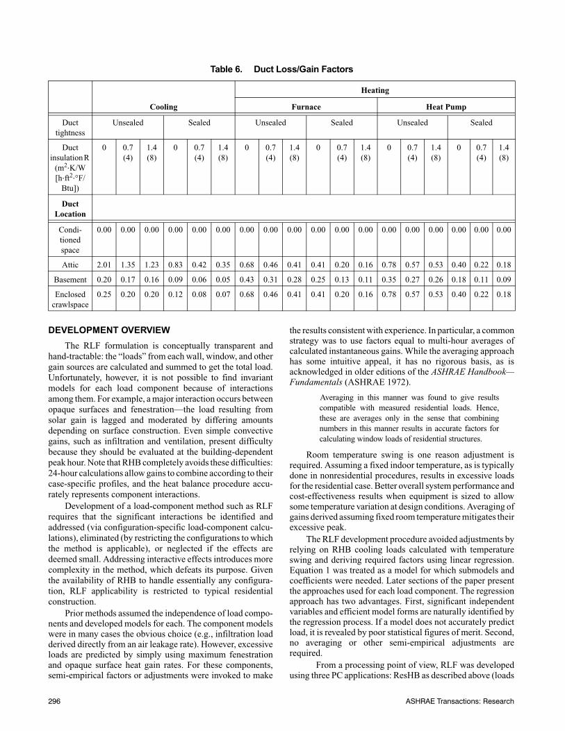
Table 6. Duct Loss/Gain Factors

Cooling

Heating

Furnace Heat Pump

Ducttightness

Unsealed Sealed Unsealed Sealed Unsealed Sealed

Ductinsulation R

(m2⋅K/W [h⋅ft2⋅°F/

Btu])

0 0.7 (4)

1.4 (8)

0 0.7 (4)

1.4 (8)

0 0.7 (4)

1.4 (8)

0 0.7 (4)

1.4 (8)

0 0.7 (4)

1.4 (8)

0 0.7 (4)

1.4 (8)

DuctLocation

Condi-tioned space

0.00 0.00 0.00 0.00 0.00 0.00 0.00 0.00 0.00 0.00 0.00 0.00 0.00 0.00 0.00 0.00 0.00 0.00

Attic 2.01 1.35 1.23 0.83 0.42 0.35 0.68 0.46 0.41 0.41 0.20 0.16 0.78 0.57 0.53 0.40 0.22 0.18

Basement 0.20 0.17 0.16 0.09 0.06 0.05 0.43 0.31 0.28 0.25 0.13 0.11 0.35 0.27 0.26 0.18 0.11 0.09

Enclosed crawlspace

0.25 0.20 0.20 0.12 0.08 0.07 0.68 0.46 0.41 0.41 0.20 0.16 0.78 0.57 0.53 0.40 0.22 0.18

296 ASHRAE Transactions: Research

calculations), RHBGen (parametric case generator), and the Rstatistics package.

RHBGen was developed to support ResHB testing andRLF development and is described by Barnaby et al. (2004).RHBGen generates and runs ResHB input files under thecontrol of multi-character parametric codes. Fields within thecode control various aspects of the case to be run, such as baseprototype (fundamental building geometry), location, orienta-tion, constructions, fenestration type and area, and so forth.RHBGen combinatorially varies code fields, allowing sets ofhundreds or thousands of ResHB runs to be constructed andexecuted. On typical Pentium-based PCs, the RHBGen/ResHB system can complete several hundred cases perminute. ResHB writes suitable results files for regression anal-ysis and other post-processing.

The R package (R 2004) is an open-source system withextensive statistical and data visualization capabilities. ForRLF development, the linear regression and data plottingprocedures were used. R is particularly suitable for RLF devel-opment because it includes a script language for automation ofcomplex analysis sequences. The R scripts used in this workcan be found in Barnaby et al. (2004).

MODELING ASSUMPTIONS

As discussed above, RLF cooling load procedures weredeveloped by using linear regression analysis of sets of ResHBresults. To generate the input data for regression, specific

combinations of inputs were varied while others were main-tained at typical values. For most variables, three levels wereidentified: L = minimum, M = typical, and H = maximum.Even with only three levels and relatively few variables, thetotal number of possible combinations is impractically large.To limit the number of cases, the range of RLF applicabilitywas restricted to conventionally constructed and occupiedsingle-family detached wood-frame buildings at latitude 20°-60° and at modest elevation. In addition, load componentswere analyzed separately, as is discussed below under“Regression Strategy.”

Prototype Building

Cooling loads for many variations of a single prototypebuilding were the basis for the regression analysis; Table 7summarizes the prototype characteristics and Table 8 showsconstruction details. The floor plan of the prototype buildingwas square with four rooms, one in each corner. Note thatResHB surfaces need not be geometrically consistent, allow-ing exterior wall area to be based on an assumed typical-widthrectangular plan and that area to be distributed equally on allfacades. The four-room plan was chosen so there was a reason-able ratio of interior partition to floor area and to limit radianttransfer among exterior walls. The sensible cooling load usedas the regression independent variable was the maximumvalue of the combined 24-hour profile derived by summing theroom loads for each hour.

Table 7. Prototype Building Characteristics

Item Value Notes

Conditioned floor area 168 m2 (1808 ft2) Typical size

Height 2.5 m (8.2 ft) Single story

Exterior wall area 142.4 m2 (1533 ft2) Average width assumed to be 8.5 m (28 ft),yielding perimeter = 57 m (187 ft)

Interior partition area 140 m2 (459 ft2) 83% of conditioned floor area

Nominal fenestration 27.2 m2 (89.2 ft2) windows1.68 m2 (18 ft2) skylight

clear double glazed (U = 2.73 W/m2K(0.48 Btu/h⋅ft2⋅F), SHGC = 0.76)

Window area = 16% of floor areaSkylight area = 1% of floor area

Fenestration variation All cases run with 200% nominal area. IAC values varied, L = 0, M = 0.5, H = 1.

Internal mass 168 m2 (1808 ft2) of 12 mm (0.5 in) wood RP-1199 default

Indoor design temperature 24°C (75.2°F)

Indoor temperature swing 1.67 K (3°F)

Infiltration Leakage class E (normalized leakage = 0.34) Reasonably tight contemporary construction (ASHRAE Standard 119, ASHRAE 1994)

Internal gain Default Based on Building America 2003, see below.

Surface exterior solar absorptance Walls: 0.6 Roof: 0-1 (varied)

Surface interior absortance Beam solar gain: floor: 0.6, internal mass: 0.3, other: 0

Diffuse solar gain: all surfaces: 0.6

Orientation 0° and 45° All 8 primary orientations considered.

ASHRAE Transactions: Research 297

Table 8. Prototype Surface Constructions

Surface ConstructionFraming Fraction

Insulation Level

U-FactorW/m2⋅K

(Btu/h⋅ft2⋅°F) Insulation Description

Ceiling Roof/ceiling, asphalt shin-gles, plywood deck, 2 × 8 framing, gypsum board

10% L 1.48005(0.26066)

None

M 0.21835(0.03846)

190 mm (7.5 in.) fiberglass between framing

H 0.11879(0.02092)

190 mm (7.5 in.) fiberglass between framing plus140 mm (5.5 in.) overlay

Attic/ceiling, 2 × 8 framing, gypsum board

10% L 2.24413(0.39523)

None

M 0.23148(0.04077)

190 mm (7.5 in.) fiberglass between framing

H 0.12204(0.02149)

190 mm (7.5 in.) fiberglass between framing plus140 mm (5.5 in.) overlay

Wall Wood frame, plywood, 2 ×

4 framing, gypsum board25% L 1.57621

(0.27760)None

M 0.50209(0.08843)

90 mm (3.5 in.) fiberglass between framing

H 0.25946(0.04570)

90 mm (3.5 in.) fiberglass between framing plus 25 mm (1 in.) foam at outside of framing

Floor Wood frame, oak floor, ply-wood deck 2 × 8 framing

10% L 0.80772(0.31837)

None

M 0.22512(0.03965)

190 mm (7.5 in.) fiberglass between framing

H 0.15737(0.02772)

190 mm (7.5 in.) fiberglass between framing plus50 mm (2 in.) foam at outside surface

Slab: 100 mm (4 in.) con-crete, 300 mm (12 in.) soil, adiabatic exterior boundary

conditions

n/a L n/a Bare slab

M n/a Additional surface resistance = 0.185 (m2⋅K)/W(1.05 [ft2⋅°F⋅h]/Btu), light carpet

H n/a Additional surface resistance = 0.370 (m2⋅K)/W(2.10 [ft2⋅°F⋅h]/Btu), heavy carpet

Table 9. Design Conditions

Case

Design Dry-Bulb Temperature

Daily Range of Dry-Bulb

Temperature

DesignWet-Bulb

Temperature

°C (°F) °C (°F) °C (°F)

LL 24 (75.2) 4 (7.2) 19 (66.2)

LM 24 (75.2) 11 (19.8) 16 (60.8)

ML 33 (91.4) 4 (7.2) 29 (84.2)

MM 33 (91.4) 11 (19.8) 23 (73.4)

MH 33 (91.4) 21 (37.8) 15 (59)

HL 43 (109.4) 4 (7.2) 24 (75.2)

HM 43 (109.4) 11 (19.8) 22 (71.6)

HH 43 (109.4) 21 (37.8) 21 (69.8)

Table 10. Site Assumptions

Item Value

Latitude 20°N, 40°N, 60°N

Longitude 75°W

Time zone –5 hr

Elevation 50 m (164 ft)

Date July 21

Time Daylight savings

Clearness 1

298 ASHRAE Transactions: Research

Outdoor Design Conditions

Eight combinations of outdoor design dry-bulb temper-ature and daily range were selected to span a broad range ofdesign conditions. Coincident wet-bulb temperatures werechosen by inspection of actual sites having design conditionssimilar to those of each combination. Table 9 summarizes thetemperature assumptions. Other site-related assumptions areshown in Table 10, most of which were held constant for allcases.

The ResHB application uses these inputs to generate 24-hour design sequences that drive the heat balance simulation.Hourly incident solar radiation was calculated using theASHRAE clear sky model (ASHRAE 2001) with updatedcoefficients (Machler and Iqbal 1985).

The combination of 8 design conditions and 3 latitudesresulted in 24 runs for each prototype variant.

REGRESSION STRATEGY

It was not practical to perform one regression analysis toidentify all RLF coefficients because of the overwhelmingnumber of case combinations that would have been required.Instead, an iterative series of linked regressions wasperformed. Equation 1 was applied to ResHB loads results andrearranged to isolate the envelope load component:

(20)

where

qenv = envelope cooling load component = in Equation 1, W (Btu/h)

qs,rhb = ResHB sensible cooling load, W (Btu/h)

qig,rhb = ResHB sensible internal gain at peak hour (simultaneous with qs,rhb), W (Btu/h)

qvi,rhb = ResHB sensible ventilation/infiltration at peak hour (simultaneous with qs,rhb), W (Btu/h)

The envelope cooling load is the sum of the load compo-nents from the various envelope elements:

(21)

Each component term of Equation 21 was estimatedusing a separate data set described in Table 11. Each data setcontains ResHB loads based on varying inputs relating to theterm under consideration while fixing other inputs at M ornominal values. The component regressions were performedin the sequence shown in Equations 22 to 25, and the resultsof each were applied to the next step. (The details of eachcomponent model are discussed below.) Initial (iteration 0)estimates were set by hand using suitable prior results. It wasdetermined by trial and error that five iterations achievedessentially complete convergence.

(22)

(23)

(24)

(25)

where

= ith iteration estimated load component for fenestration, ceiling, wall, or floor, W (Btu/h)

COMPONENT MODELS

Ventilation and Infiltration

As discussed above, typical infiltration was included inthe ResHB runs used to generate regression data, but the cool-ing load induced by this air leakage was subtracted from theload used in the envelope regressions. Thus, the loads

Table 11. Regression Data Sets

Component Fenestration Ceiling Wall Floor

Total Cases(24 design conditions,

2 orientations)

qfen 41 combinations of LMH on 4 facades plus skylight (Box-Behnkin 5 factor design)

Attic, M∝roof = 0.85

Wood frame, M Crawlspace, MExposed, MSlab, M

5904

qceil Nominal Roof/ceiling LMH, Attic LMH, each with∝roof = 0, 0.6, 1

Wood frame, M Crawlspace, MExposed, MSlab, M

2592

qwall Nominal Attic, M∝roof = 0.85

Wood frame, LMH Crawlspace, MExposed, MSlab, M

432

qfloor Nominal Attic, M∝roof= 0.85

Wood frame, M Crawlspace, LMHExposed, LMHSlab, LMH

432

qenv qs ,rhb qig ,rhb– qvi ,rhb–=

Ai CFi⋅∑

qenv qfen qceil qwall qfloor+ + +=

q̂feni 1+

qenv q̂ceili

– q̂walli

– q̂floori

–=

q̂ceili 1+

qenv q̂feni 1+

– q̂walli

– q̂floori

–=

q̂walli 1+

qenv q̂feni 1+

– q̂ceili 1+

– q̂floori

–=

q̂floori 1+

qenv q̂feni 1+

– q̂ceili 1+

– q̂walli 1+

–=

q̂xi

ASHRAE Transactions: Research 299

predicted by the regression models implicitly assume 0 airleakage.

Equation 9 was developed to provide a simple method forestimating infiltration leakage for RLF. ResHB calculatesinfiltration using the AIM-2 model (Walker and Wilson 1990,1998), which is too complex for practical hand application.The AIM-2 model was exercised over a range of temperaturedifferences and building heights. Other assumptions includedshelter class 4, flue shelter class 2, and wind speed multipliervalues from Table 10, Chapter 26, ASHRAE (2001). Leakagedistribution was assumed to be walls = 0.5, ceiling = 0.25,floor = 0.25 (R = 1, X = 0), all proportionately reduced if flueis present. The maximum flue leakage fraction considered was0.5. Regression was used to find the form of Equation 9 and theIx coefficients. The underlying functional form of the AIM-2model is not linear, but the simple form of Equation 9 wasmaintained for ease of application. The regression modelyielded an adjusted R2 of 0.94. Figure 1 compares results fromthe regression to those from AIM-2. Because of minimal airdensity dependence, Equation 9 is valid at any elevation.

The procedure for combining mechanical ventilation withinfiltration airflows, shown in Equations 10 to 12, follows(Palmiter and Bond 1991; Sherman 1992).

Internal Gains

RHB internal gains are based on Building America(2003), which specifies gain intensities and schedules for resi-dential appliances, lighting, and occupants. Experiments with

these gains and schedules in ResHB revealed that the sensiblecooling load attributable to internal gains is generally approx-imated by the total sensible internal gain during the peak cool-ing hour. This is not necessarily expected, since a significantfraction of the gain is radiant and has a delayed load impact.The removal of load due to internal gain in Equation 20 isbased on this approximation.

For RLF, Equations 17 and 18 are the aggregated BuildingAmerica gains using 4 PM schedule values, that time being acommon peak cooling hour for typical residential construc-tion. Consideration was given to developing a model thatpredicts the peak cooling hour so a more accurate internalgains formulation could be included. However, such an addi-tion to RLF was deemed excessively complex.

Opaque Surfaces

The model forms for opaque surface CFs were found byexperimentation. Prior methods—both residential and non-residential—have used an equivalent temperature difference(ETD) or cooling load temperature difference (CLTD) form,where ETD or CLTD = A + ∆T – DR/2, where A is a constant,∆T is the outdoor-indoor temperature difference, and DR is thedaily range). This was taken as a starting point for RLF. Acoefficient was added for ∆T, and multipliers other than 0.5were allowed for DR. In some cases, the ∆T coefficient wasfound to be a value very close to 1, in which case it wasdropped from the regression and forced to be 1. In other cases,coefficients were found to be not significant and dropped. TheDR coefficient takes many values, indicating that the tradi-tional 0.5 is perhaps not ideal. The final coefficient values areshown in Table 1. Adjusted R2 values for all regressions wereabove 0.96.

A major design consideration was how many surfacetypes to include. It was decided to limit RLF to conventionalwood-frame construction. That led to inclusion of one type ofwall (wood frame), two types of ceilings (ceiling/roof and ceil-ing/attic combinations), and three types of floors (exposed,crawlspace, and slab). Surface orientation was not a variable(all wall orientations are combined) and solar absorptance wastreated as a variable only for roofs. It is believed that additionalsurface types could be added via straightforward extension ofthe current procedures.

Fenestration

A goal for the fenestration model was the separation oflatitude-dependent exterior effects from building-dependenteffects. It was determined by experimentation that this isachieved by factoring out peak hour irradiance incident on thefenestration exterior, leading the PXI formulation shown inEquation 5. As with the opaque surface models, this form issimilar to prior residential and nonresidential methods. Manycombinations of effective window aperture were included in

Figure 1 Predicted infiltration leakage rates, AL = 1000cm2 (155 in.2), and representative range of stackheight, temperature difference, and flue fraction.RLF values from Equation 9; see text (1 L/s = 2.12cfm).

300 ASHRAE Transactions: Research

the regression data set used to find the FFs coefficients. Thefinal adjusted R2 value was over 0.995.

An attempt was made to eliminate exposure-specific FFsvalues, leaving PXI as the only exposure-dependent input.This produced significantly worse regression results. The FFscoefficients (Table 2) show a physically reasonable relation-ship with exposure. East surfaces produce less cooling loadper unit irradiance than do west surfaces, as is expected. Priormethods that relied on averaging show a less plausible E/Wand SE/SW symmetry.

Distribution Losses

Duct losses can be calculated using models specified inASHRAE (2004) and Palmiter and Francisco (1997). Thesemodels are fully implemented in the ResHB. Using typicalinput values, ResHB was exercised to produce Table 6 suitablefor use with RLF hand calculations.

HEATING LOADS

The RLF procedure for heating loads calculation is iden-tical, in most respects, to previously published ASHRAE(2001) residential heating load calculation procedures. Theheating load calculation is based on a steady-state UA∆Tcalculation, with no solar radiation and no internal heat gains.Infiltration leakage rate is based on Equation 9. The calcula-tion procedure for heat losses from surfaces in contact with theground has been revised as described in the following sections.

Basement Wall Heat Losses

For basement wall and floor heat transfer, the ASHRAEHandbook—Fundamentals has incorporated a proceduredescribed by Latta and Boileau (1969) for a number of years.The Latta and Boileau method has the advantage of simplicity.

One check of its accuracy was described by Sobotka et al.(1994), who showed that the Latta and Boileau method under-predicted the peak heating load of one basement by 16%.Correlation-based methods (Krarti and Choi 1996; Beauso-leil-Morrison and Mitalas 1997) have been developed thatoffer significantly improved accuracy. However, these latermethods have a large number of coefficients, which compli-cates presentation in a handbook. Therefore, the RLF proce-dure has incorporated a revised version of the Latta andBoileau procedure with the suggestion that buildings wherethe heating loads are significantly impacted by ground heattransfer should be analyzed with one of the more accuratemethods.

The Latta and Boileau method is based on the assump-tions that the surface temperature of the ground is at a calcu-lable winter design temperature and that the heat flow pathsmay be approximated as circumferential with radial isotherms(see Figure 2). It also assumes that the thermal resistance of theground may be estimated based on the path length of the heattransfer. In the original Latta and Boileau (1969) paper, tabu-lated U-factors included inside thermal resistance, thermalresistance of a concrete wall, thermal resistance of insulation(if any), and thermal resistance of the soil. The tabulatedvalues were based on a coarse numerical integration and werespecific to single combinations of soil thermal conductivityand insulation thermal resistance. The approach taken in thetables also depends on the interval value for the numeric inte-gration being one foot. This presentation has been, at times,somewhat confusing. In fact, the values in the SI version of the2001 ASHRAE Handbook—Fundamentals are wrong, appar-ently having been misconverted due to the dependence on theinterval. In addition, at some point, the original Latta andBoileau recommendation to use a ground temperature calcu-lated as the mean ground temperature minus the annual ampli-tude, A, was re-expressed to use a ground temperaturecalculated as the average winter air temperature minus theannual amplitude. This results in significant overprediction ofthe ground heat loss.

In the RLF procedure, the original Latta and Boileau workwas revisited and reformulated in a more flexible manner. Therevised procedure allows for variation of the soil thermalconductivity and, if desired, partial wall insulation with anythermal resistance. Furthermore, an analytical expression forthe average U-factor has been developed, along with newtables. This may be summarized as follows.

In cases where the basement wall is partially insulated, itwill be desirable to calculate the heat loss separately forportions of the wall with differing amounts of insulation.Consider the region between depth z1 and z2 in Figure 3. (Herez1 and z2 can be any region of the wall, including the entirewall.)

For the region of interest, in steady-state heat transfer,there are several thermal resistances of interest—the soil, theconcrete wall, the insulation (if any), and the inside surfaceresistance. If all thermal resistances besides the soil are

Figure 2 Heat flow from basements (ASHRAE 2001).

ASHRAE Transactions: Research 301

lumped into a single value, Rother, the average U-factorbetween the basement air and the ground temperature is

(26)

where

Uavg,bw = average U-factor between basement air and ground temperature over region of interest shown in Figure 3, W/m2⋅K (Btu/h⋅ft2⋅°F);

ksoil = soil thermal conductivity, W/m⋅K (Btu/h⋅ft⋅°F);

z1 = depth of upper bound of region of interest (see Figure 3), m (ft);

z2 = depth of lower bound of region of interest (see Figure 3), m (ft); and

Rother = combined resistance of wall, insulation, and surface conductance, m2⋅K/W (ft2⋅h⋅F/Btu).

While values of soil conductivity vary widely with soiltype and moisture content, a typical value of 1.4 W/m⋅K (0.8Btu/h⋅ft⋅°F) was used in past editions of the ASHRAE Hand-book—Fundamentals to tabulate U-factors. Rother is the sum ofthe resistance of the concrete wall, insulation (if any), and theinside surface resistance. In past editions of the ASHRAEHandbook—Fundamentals, Rother was approximately0.25 m2⋅K/W (1.47 ft2⋅h⋅°F/Btu) for uninsulated concretewalls. For these parameters, Uavg,bw is tabulated for a range ofdepths and insulation levels in Table 12.

Basement Floor Heat Losses

The RLF procedure uses an analogously updated versionof the Latta and Boileau procedure for basement floors. Forcases where the entire basement floor is uninsulated or hasuniform insulation, the average U-factor is

(27)

where

Uavg,bf = average U-factor between basement air and ground temperature for entire basement floor, W/m2⋅°K (Btu/h⋅ft2⋅°F);

ksoil = soil thermal conductivity, W/m⋅K (Btu/h⋅ft⋅°F);

Wb = basement width, which should be taken to be the shortest dimension, m (ft);

zf = depth of slab bottom (see Figure 3), m (ft); and

Rother = combined resistance of floor, insulation and surface conductance, m2⋅K/W (ft2⋅h⋅°F/Btu).

For a soil conductivity of 1.4 W/m⋅K (0.8 Btu/h⋅ft⋅°F),Uavg,bf for uninsulated basement floors are tabulated inTable 13.

Slab-on-Grade Floor Heat Losses

Concrete slab floors have been previously approximatedas having heat losses solely proportional to the perimeterlength by Wang (1979) and Bligh et al. (1978). More recentwork (Bahnfleth and Pedersen 1990) has shown a significanteffect of the area-to-perimeter ratio. The correlation-basedmethods for basement wall and floor heat transfer describedabove (Krarti and Choi 1996; Beausoleil-Morrison andMitalas 1997) also have procedures for dealing with a widerange of slab-on-grade configurations. Again, if slab heat lossis a significant factor in the building heating load, one of theseprocedures should be used. However, for Handbook presenta-tion, the previous approach was retained, with the exceptionthat the table that showed some dependence of the perimeterheat loss factor on the number of degree-days was simplifiedby eliminating the degree-day dependence.

The simplified approach gives heat loss for both unheatedand heated slab floors with the following equation:

Figure 3 Definition of basement wall and floor dimensions.

Uavg ,bw

2ksoil

π z2

z1

–( )------------------------- z

2

2ksoil

Rother

π-----------------------------------+⎝ ⎠

⎛ ⎞ln z1

2ksoil

Rother

π-----------------------------------+⎝ ⎠

⎛ ⎞ln– ,=

Uavg,bf

2ksoil

πWb

--------------Wb

2-------

zf

2---

ksoilRother

π--------------------------+ +⎝ ⎠

⎛ ⎞lnzf

2---

ksoilRother

π--------------------------+⎝ ⎠

⎛ ⎞ln– ,=

302 ASHRAE Transactions: Research

Table 12a. Average U-Factor for Basement Walls with Uniform Insulation (SI Units)

Uavg,bw from Grade to Depth, W/m2⋅K*

Depth (m) Uninsulated R-0.88 R-1.76 R-2.64

0.3 2.468 0.769 0.458 0.326

0.6 1.898 0.689 0.427 0.310

0.9 1.571 0.628 0.401 0.296

1.2 1.353 0.579 0.379 0.283

1.5 1.195 0.539 0.360 0.272

1.8 1.075 0.505 0.343 0.262

2.1 0.980 0.476 0.328 0.252

2.4 0.902 0.450 0.315 0.244

* Soil conductivity is 1.4 W/m-K; insulation is over entire depth. For other soil conductivities and partial insulation, use equations.

Table 12b. Average U-Factor for Basement Walls with Uniform Insulation (I-P Units)

Uavg,bw from Grade to Depth, Btu/h⋅ft2⋅°F*

Depth (ft) Uninsulated R-5 R-10 R-15

1 0.432 0.135 0.080 0.057

2 0.331 0.121 0.075 0.054

3 0.273 0.110 0.070 0.052

4 0.235 0.101 0.066 0.050

5 0.208 0.094 0.063 0.048

6 0.187 0.088 0.060 0.046

7 0.170 0.083 0.057 0.044

8 0.157 0.078 0.055 0.043

* Soil conductivity is 0.8 Btu/h⋅ft⋅°F; insulation is over entire depth. For other soil conductivities and partial insulation, use equations.

Table 13a. Average U-Factor for Basement Floors (SI Units)

zf (depth of foundation wall below grade), m

Uavg,bf, W/m2K*

Wb (shortest width of basement), m

6 7 8 9

0.3 0.370 0.335 0.307 0.283

0.6 0.310 0.283 0.261 0.242

0.9 0.271 0.249 0.230 0.215

1.2 0.242 0.224 0.208 0.195

1.5 0.220 0.204 0.190 0.179

1.8 0.202 0.188 0.176 0.166

2.1 0.187 0.175 0.164 0.155

* Soil conductivity is 1.4 W/m⋅K; floor is uninsulated. For other soil conductivities and partial insulation, use equations.

ASHRAE Transactions: Research 303

Table 13b. Average U-Factor for Basement Floors (I-P Units)

zf (depth of foundation wall below grade), ft

Uavg,bf, Btu/h-ft2-°F*

Wb (shortest width of basement), ft

20 24 28 32

1 0.064 0.057 0.052 0.047

2 0.054 0.048 0.044 0.040

3 0.047 0.042 0.039 0.036

4 0.042 0.038 0.035 0.033

5 0.038 0.035 0.032 0.030

6 0.035 0.032 0.030 0.028

7 0.032 0.030 0.028 0.026

* Soil conductivity is 0.8 Btu/h⋅ft⋅°F; floor is uninsulated. For other soil conductivities and partial insulation, use equations.

Table 14a. Heat Loss Coefficient F2 of Slab Floor Construction (SI Units)

Construction Insulation F2 (W/K-m)

200 mm. block wall,brick facing

Uninsulated 1.17

R-0.95 K-m2/W fromedge to footer

0.86

200 mm. block wall,brick facing

Uninsulated 1.45

R-0.95 K-m2/W fromedge to footer

0.85

Metal stud wall,stucco

Uninsulated 2.07

R-0.95 K-m2/W fromedge to footer

0.92

Poured concrete wallwith duct nearperimetera

Uninsulated 3.67

R-0.95 K-m2/W fromedge to footer

1.24

aWeighted average temperature of the heating duct was assumed at 43°C duringthe heating season (outdoor air temperature less than 18°C)

Table 14b. Heat Loss Coefficient F2 of Slab Floor Construction (I-P Units)

Construction Insulation F2 (Btu/h-ft-°F)

8 in. block wall,brick facing

Uninsulated 0.68

R-5.4 fromedge to footer

0.50

4 in. block wall,brick facing

Uninsulated 0.84

R-5.4 fromedge to footer

0.49

Metal stud wall,stucco

Uninsulated 1.20

R-5.4 fromedge to footer

0.53

Poured concrete wallwith duct nearperimetera

Uninsulated 2.12

R-5.4 fromedge to footer

0.72

aWeighted average temperature of the heating duct was assumed at110°F during the heating season (outdoor air temperature less than65°F).

304 ASHRAE Transactions: Research

(28)

where

q = heat loss through perimeter, W (Btu/h)

F2 = heat loss coefficient per unit length of perimeter,W/m⋅K (Btu/h⋅ft⋅°F) (see Table 14)

P = perimeter or exposed edge of floor, m (ft)

∆T = heating design temperature difference, K (°F)

Noting that the degree-day dependence previously givenin the ASHRAE Handbook—Fundamentals is relatively small,the table of F2 factors was simplified by only giving the valuefor 2970 Kelvin degree-day (5350 Fahrenheit degree-day)climates.

VERIFICATION OF RESULTS

The RLF method was added to the ResHB application,allowing RLF vs. RHB cooling load calculations to beperformed on test cases. Figure 4 shows typical results of sucha comparison for a building not involved in the regressionprocess and using design weather data for 20 diverse US loca-tions. As can be seen, there is generally good agreement but atrend remains in that RLF predicts too high for low loads andtoo low for high loads. This is being investigated and may leadto model refinement.

CONCLUSIONS

A number of conclusions can be drawn from this work:

• Linear regression is a useful tool for devising simplifiedbuilding cooling load prediction models. Regressionobviates the need for averaging and other semi-empiri-cal adjustments. Further, it appears that reasonablyaccurate regression models can be found for virtuallyany building configuration.

• On the other hand, all simplified models having the RLFform (including RLF) have the distinct disadvantagethat they do not give any indication of when theybecome inapplicable. For example, the peak coolinghour cannot be identified from the RLF procedure; if thepeak is shifted, the internal gain load component couldbe significantly in error.

• Even within the range of applicability, uncertainty onthe order of 1000 W (0.25 ton) is expected with RLF-style models. This uncertainty could be reduced viaaddition of model refinements. However, adding com-plexity to RLF defeats its purpose as a hand-tractablemethod while not achieving the accuracy and flexibilityof RHB.

ACKNOWLEDGMENTS

The authors thank Bruce A. Wilcox for helpful discus-sions regarding the regression techniques and Phil Sobolik fordevelopment of automated regression procedures.

NOMENCLATURE

A = area, m2 (ft2)

AL = building effective leakage area (including flue) at 4 Pa assuming CD = 1, cm2 (in.2)

Cl = air latent heat factor, 3010 W/(L/s) (4840 Btu/h⋅cfm) at sea level

Cs = air sensible heat factor, 1.23 W/(L/s)⋅K(1.1 Btu/h⋅cfm⋅°F) at sea level

Ct = air total heat factor, 1.2 W/(L/s)-(kJ/kg)(4.5 Btu/h⋅cfm⋅[Btu/lb]) at sea level

CF = cooling (load) factor, W/m2 (Btu/h⋅ft2)

Doh = depth of overhang (from plane of fenestration), m (ft)

DR = daily range of outdoor dry-bulb temperature, K (°F)

E = peak irradiance for exposure, W/m2 (Btu/h⋅ft2)

F2 = heat loss coefficient per unit length of perimeter (see Table 14), W/m⋅K (Btu/h⋅ft⋅°F)

Fdl = distribution loss factor

Fshd = fraction of fenestration shaded by permanent overhangs, fins, or environmental obstacles

FF = coefficient for CFfen

G = internal gain coefficient

hsrf = effective surface conductance, including resistance of slab covering material such as carpet, W/m2⋅K (Btu/h⋅ft2⋅°F). 1/(Rcvr + 0.12) W/m2⋅K or1/(Rcvr + 0.68) Btu/h⋅ft2⋅°F

H = height

q F2 P T∆⋅ ⋅=

Figure 4 RLF vs. RHB sensible cooling load comparison.Test building calculated for representative rangeof climate and construction conditions (1280cases).

ASHRAE Transactions: Research 305

HF = heating (load) factor, W/m2 (Btu/h⋅ft2)

I = infiltration coefficient

IAC = interior shading attenuation coefficient

k = conductivity, W/m⋅K (Btu/h⋅ft⋅°F)

LF = load factor, W/m2 (Btu/h⋅ft2)

OF = coefficient for CFopq

P = perimeter or exposed edge of floor, m (ft)

PXI = peak exterior irradiance, including shading modifications, W/m2 (Btu/h⋅ft2)

q = heating or cooling load, W (Btu/h)

Q = air volumetric flow rate, L/s (cfm)

R = insulation thermal resistance, m2⋅K/W (h⋅ft2⋅°F/Btu)

SHGC = fenestration rated or estimated NFRC solar heat gain coefficient

SLF = shade line factor

Tx = solar transmission of exterior attachment, see Table 4

U = construction U-factor, W/m2⋅K (Btu/h⋅ft2⋅°F); for fenestration, NFRC rated heating U-factor

W = width, m (ft)

Xoh = vertical distance from top of fenestration to overhang, m (ft)

z = depth below grade, m (ft)

Greek Symbols

αroof = roof solar absorptance

∆h = indoor-outdoor enthalpy difference, kJ/kg

∆T = design dry-bulb temperature difference (outdoor-indoor), K (°F)

∆W = indoor-outdoor humidity ratio difference

ε = heat/energy recovery ventilation (HRV/ERV) effectiveness

Subscripts

avg = average

b = base (as in OFb) or basement

bal = balanced

bf = basement floor

bw = basement wall

ceil = ceiling

cf = conditioned floor

d = diffuse

D = direct

dl = distribution loss

env = envelope

exh = exhaust

fen = fenestration

floor = floor

hr = heat recovery

ig = internal gain

inf = infiltration

l = latent

oc = occupant

oh = overhang

opq = opaque

oth = other

r = daily range (as in OFr)

rhb = calculated with RHB method

s = sensible

shd = shaded

slab = slab

srf = surface

sup = supply

t = total or temperature (as in OFt)

unbal = unbalanced

vi = ventilation / infiltration

wall = wall

REFERENCES

ACCA. 1986. Manual J, Load Calculation for ResidentialWinter and Summer Air Conditioning, 7th ed. Arlington,Va.: Air Conditioning Contractors of America.

ACCA. 2003. Manual J, Residential Load Calculations, 8thed. Arlington, Va.: Air Conditioning Contractors ofAmerica.

ASHRAE. 1972. 1972 ASHRAE Handbook—Fundamen-tals. New York: American Society of Heating, Refriger-ating and Air-Conditioning Engineers, Inc.

ASHRAE. 1994. ANSI/ASHRAE Standard 119-1988 (RA94), Air Leakage Performance of Detached Single-Fam-ily Residential Buildings. Atlanta: American Society ofHeating, Refrigerating and Air-Conditioning Engineers,Inc.

ASHRAE. 2001. 2001 ASHRAE Handbook—Fundamen-tals. Atlanta: American Society of Heating, Refrigerat-ing and Air-Conditioning Engineers, Inc.

ASHRAE. 2004. ANSI/ASHRAE 152-2004, Method of Testfor Determining the Design and Seasonal Efficiencies ofResidential Thermal Distribution Systems. Atlanta:American Society of Heating, Refrigerating and Air-Conditioning Engineers, Inc.

ASHRAE. 2005. 2005 ASHRAE Handbook—Fundamen-tals. Atlanta: American Society of Heating, Refrigerat-ing and Air-Conditioning Engineers, Inc.

Bahnfleth, W.P., and C.O. Pedersen. 1990. A three-dimen-sional numerical study of slab-on-grade heat transfer.ASHRAE Transactions 96(2):61-72.

Barnaby, C.S., J.D. Spitler, and D. Xiao. 2004. Updating theASHRAE/ACCA Residential Heating and CoolingLoad Calculation Procedures and Data, RP-1199 FinalReport. Atlanta: American Society of Heating, Refriger-ating and Air-Conditioning Engineers, Inc.

306 ASHRAE Transactions: Research

Barnaby, C.S., J.D. Spitler, and D. Xiao. 2005. The residen-tial heat balance method for heating and cooling loadcalculations (RP-1199). ASHRAE Transactions 111(1).Atlanta: American Society of Heating, Refrigeratingand Air-Conditioning Engineers, Inc.

Beausoleil-Morrison, I., and G. Mitalas. 1997. BASESIMP:A residential-foundation heat-loss algorithm for incor-porating into whole-building energy-analysis programs.Building Simulation ’97, Prague.

Bligh, T.P., P. Shipp, and G. Meixel. 1978. Energy compari-sons and where to insulate earth sheltered buildings andbasements. Earth covered settlements, U.S. Departmentof Energy Conference, Fort Worth, Texas.

Brunger, A., F. Dubrous, and S. Harrison. 1999. Measure-ment of the solar heat gain coefficient and U-value ofwindows with insect screens. ASHRAE Transactions105(2). Atlanta: American Society of Heating, Refriger-ating and Air-Conditioning Engineers, Inc.

Building America. 2003. Building America Research Bench-mark Definition, Version 3.1. Available at http://www.eere.energy.gov/buildings/building_america/pdfs/benchmark_def_ver3.pdf.

CSA. 1990. CAN/CSA-F280-M90, Determining theRequired capacity of Residential space Heating andCooling Appliances. Canadian Standards Association,Rexdale (Toronto), ON, Canada.

HRAI. 1996. Residential Heat Loss and Gain Calculations,Student Reference Guide. Mississauga, ON, Canada:Heating, Refrigerating and Air Conditioning Institute ofCanada.

Krarti, M., and S. Choi. 1996. Simplified method for founda-tion heat loss calculation. ASHRAE Transactions102(1):140-152.

Latta, J.K., and G.G. Boileau. 1969. Heat losses from housebasements. Canadian Building 19(10):39.

Machler, M.A., and Iqbal, M. 1985. A modification of theASHRAE clear sky irradiation model. ASHRAE Trans-actions 91(1A):106-115.

McQuiston, F.C. 1984. A study and review of existing datato develop a standard methodology for residential heat-ing and cooling load calculations, RP-342. ASHRAETransactions 90(2A):102-36.

Palmiter, L., and T. Bond. 1991. Interaction of mechanicalsystems and natural infiltration. Proceedings of the 12thAIVC Conference on Air Movement and VentilationControl Within Buildings, Air Infiltration and Ventila-tion Centre, Coventry, Great Britain.

Palmiter, L., and P. Francisco. 1997. Development of a prac-tical method of estimating the thermal efficiency of resi-dential forced-air distribution systems, EPRI report TR-107744. Electric Power Research Institute, Palo Alto,Calif.

Pedersen, C.O., D.E. Fisher, and R.J. Liesen. 1997. A heatbalance based cooling load calculation procedure.ASHRAE Transactions 103(2):459-468.

Pedersen, C.O., D.E. Fisher, J.D. Spitler, and R.J. Liesen.1998. Cooling and Heating Load Calculation Princi-ples. Atlanta: American Society of Heating, Refrigerat-ing and Air-Conditioning Engineers, Inc.

Pedersen, C.O., R.J. Liesen, R.K. Strand, D.E. Fisher, L.Dong, and P.G. Ellis. 2001. A Toolkit for Building LoadCalculations. Atlanta: American Society of Heating,Refrigerating and Air-Conditioning Engineers, Inc.

R. 2004. Open source software available at http://www.r-project.org/.

Sherman, M.H. 1992. Superposition in infiltration modeling.Indoor Air 2:101-14.

Sobotka, P., H. Yoshino, et al. 1994. Thermal performance ofthree deep basements: A comparison of measurementswith ASHRAE Fundamentals and the Mitalas method,the European Standard and the two-dimensional FEMprogram. Energy and Buildings 21:23-34.

Walker, I.S., and D.J. Wilson. 1998. Field validation of equa-tions for stack and wind driven air infiltration calcula-tions. International Journal of HVAC&R Research 4(2).

Walker, I.S., and D.J. Wilson. 1990. The Alberta Air Infiltra-tion Model. The University of Alberta, Department ofMechanical Engineering, Technical Report 71.

Wang, F.S. 1979. Mathematical modeling and computer sim-ulation of insulation systems in below grade applica-tions. ASHRAE/DOE Conference on ThermalPerformance of the Exterior Envelopes of Buildings,Orlando, Florida.

ASHRAE Transactions: Research 307

This paper has been downloaded from the Building and Environmental Thermal Systems Research Group at Oklahoma State University (www.hvac.okstate.edu) The correct citation for the paper is: Barnaby, C.S., J.D. Spitler. 2005. Development of the Residential Load Factor Method for Heating and Cooling Load Calculations. ASHRAE Transactions, 111(1):291-307. Reprinted by permission from ASHRAE Transactions (Vol. #11, Number 4, pp. 637-655). © 2004 American Society of Heating, Refrigerating and Air-Conditioning Engineers, Inc.