Embed Size (px)
Citation preview

VERSION 4.4
Structural Mechanics ModuleModel Library Manual

C o n t a c t I n f o r m a t i o n
Visit the Contact COMSOL page at www.comsol.com/contact to submit general inquiries, contact Technical Support, or search for an address and phone number. You can also visit the Worldwide Sales Offices page at www.comsol.com/contact/offices for address and contact information.
If you need to contact Support, an online request form is located at the COMSOL Access page at www.comsol.com/support/case.
Other useful links include:
• Support Center: www.comsol.com/support
• Product Download: www.comsol.com/support/download
• Product Updates: www.comsol.com/support/updates
• COMSOL Community: www.comsol.com/community
• Events: www.comsol.com/events
• COMSOL Video Center: www.comsol.com/video
• Support Knowledge Base: www.comsol.com/support/knowledgebase
Part number: CM021102
S t r u c t u r a l M e c h a n i c s M o d u l e M o d e l L i b r a r y M a n u a l © 1998–2013 COMSOL
Protected by U.S. Patents 7,519,518; 7,596,474; 7,623,991; and 8,457,932. Patents pending.
This Documentation and the Programs described herein are furnished under the COMSOL Software License Agreement (www.comsol.com/sla) and may be used or copied only under the terms of the license agreement.
COMSOL, COMSOL Multiphysics, Capture the Concept, COMSOL Desktop, and LiveLink are either registered trademarks or trademarks of COMSOL AB. All other trademarks are the property of their respective owners, and COMSOL AB and its subsidiaries and products are not affiliated with, endorsed by, sponsored by, or supported by those trademark owners. For a list of such trademark owners, see www.comsol.com/tm.
Version: November 2013 COMSOL 4.4

Solved with COMSOL Multiphysics 4.4
F l u i d - S t r u c t u r e I n t e r a c t i o n i n A l um i num Ex t r u s i o n
Introduction
Out of all metals, the most frequently extruded is aluminum. Aluminum extrusion entails using a hydraulic ram to squeeze an aluminum bar through a die. This process will form the metal into a particular shape. Extruded aluminum is used in many manufacturing applications, such as building components for example. In massive forming processes like rolling or extrusion, metal alloys are deformed in a hot solid state with material flowing under ideally plastic conditions. Such processes can be simulated effectively using computational fluid dynamics, where the material is considered as a fluid with a very high viscosity that depends on velocity and temperature. Internal friction of the moving material acts as a heat source, so that the heat transfer equations are fully coupled with those ruling the fluid dynamics part. This approach is especially advantageous when large deformations are involved.
This model is adapted from a benchmark study in Ref. 1. The original benchmark solves a thermal-structural coupling, because it is common practice in the simulation of such processes to use specific finite element codes that have the capability to couple the structural equations with heat transfer. The alternative scheme discussed here couples non-Newtonian flow with heat transfer equations. In addition, because it is useful to know the stress in the die due to fluid pressure and thermal loads, the model adds a structural mechanics analysis.
The die design is courtesy of Compes S.p.A., while the die geometry, boundary conditions, and experimental data are taken from Ref. 1.
Note: This model requires the Heat Transfer Module and the Structural Mechanics Module. In addition, the model uses the Material Library.
1 | F L U I D - S T R U C T U R E I N T E R A C T I O N I N A L U M I N U M E X T R U S I O N

Solved with COMSOL Multiphysics 4.4
2 | F L U
Model Definition
The model considers steady-state conditions, assuming a billet of infinite length flowing through the die. In the actual process, the billet is pushed by the ram through the die and its volume is continuously reducing.
Figure 1 shows the original complete geometry with four different profiles. To have a model with reasonable dimensions, consider only a quarter of the original geometry. The simplification involved in neglecting the differences between the four profiles does not affect the numerical scheme proposed. Figure 2 shows the resulting model
I D - S T R U C T U R E I N T E R A C T I O N I N A L U M I N U M E X T R U S I O N

Solved with COMSOL Multiphysics 4.4
geometry.
Figure 1: Original benchmark geometry.
Figure 2: Quarter of the original geometry considered in the model.
M A T E R I A L P R O P E R T I E S
The documentation for the benchmark model (Ref. 1) serves as the data source for properties of the two main materials: AISI steel for the die and the container (the ram is not considered here) and aluminum for the billet.
3 | F L U I D - S T R U C T U R E I N T E R A C T I O N I N A L U M I N U M E X T R U S I O N

Solved with COMSOL Multiphysics 4.4
4 | F L U
Structural AnalysisBecause only the steel part is active in the structural analysis, consider a simple linear elastic behavior where the elastic properties are those of the material H11 mod (AISI 610) that can be found in the COMSOL Multiphysics Material Library.
Heat Transfer AnalysisThe benchmark model uses the following properties for aluminum and steel:
Non-Newtonian FlowThe properties of the aluminum were experimentally determined and then checked using literature data for the same alloy and surface state. However the benchmark proposes an experimental constitutive law, suited for the structural mechanics codes usually used to simulate such processes, in the form of the flow stress data. For this model this requires a recalculation of the constitutive law to derive a general expression for the viscosity. The equivalent von Mises stress, eqv, can be defined in terms of the total contraction of the deviatoric stress tensor as
or, using where is the strain rate and is the viscosity, as
(1)
Introducing the equivalent strain rate
Equation 1 can be expressed as
ALUMINUM VALUE DESCRIPTION
kal 210 N/(s·K) Thermal conductivity
al 2700 kg/m3 Density
Cpal 2.94 N/(mm2·K)/al Specific heat
STEEL VALUE DESCRIPTION
kfe 24.33 N/(s·K) Thermal conductivity
fe 7850 kg/m3 Density
Cpfe 4.63 N/(mm2·K)/fe Specific heat
eqv32---:=
2·= ·
eqv 62· :·=
· eqv23---· :·
I D - S T R U C T U R E I N T E R A C T I O N I N A L U M I N U M E X T R U S I O N

Solved with COMSOL Multiphysics 4.4
The strain rate tensor is defined as (Ref. 2)
The shear rate is defined as
so that
The flow rule
states that plastic yielding occurs if the equivalent stress, eqv, reaches the flow stress, f. The viscosity is defined as (see Ref. 2 for further details)
The organizers of the benchmark propose specific flow-stress data expressed in terms of a generalized Zener-Hollomon function
where A2.39·108 s1, n2.976, 0.052MPa1, and
with Q 153 kJ/mol and R8.314 J/(K·mol).
eqv 3· eqv=
· u u T+2
------------------------------- 12---·= =
·
· · 12---· :·= =
eqv13
-------·=
eqv f=
f
3· eqv--------------=
ZA----
1n---
asinh
3·----------------------------------=
Z 13
-------·e
QRT---------
=
5 | F L U I D - S T R U C T U R E I N T E R A C T I O N I N A L U M I N U M E X T R U S I O N

Solved with COMSOL Multiphysics 4.4
6 | F L U
S O U R C E S , I N I T I A L C O N D I T I O N S , A N D B O U N D A R Y C O N D I T I O N S
Structural AnalysisBecause the model geometry is a quarter of the actual geometry, use symmetric boundary conditions for the two orthogonal planes. On the external surfaces of the die, apply roller boundary conditions because in reality other dies, not considered here, are present to increase the system’s stiffness.
The main loads are the thermal loads from the heat transfer analysis and pressures from the fluid dynamics analysis.
Heat Transfer AnalysisFor the billet, use a volumetric heat source related to the viscous heating effect.
The external temperature of the ram and the die is held constant at 450 C (723 K). The ambient temperature is 25 C (298 K). For the heat exchange between aluminum and steel, use the heat transfer coefficient of 11 N/(s·mm·K). Also consider convective heat exchange with air outside the profiles with a fixed convective heat transfer coefficient of 15 W/(m2·K).
Apply initial temperatures as given in the following table:
Non-Newtonian FlowAt the inlet, the ram moves with a constant velocity of 0.5 mm/s. Impose this boundary condition by simply applying a constant inlet velocity. At the outlet, a normal stress condition with zero external pressure applies. On the surfaces placed on the two symmetry planes, use symmetric conditions. Finally, apply slip boundary conditions on the boundaries placed outside the profile.
Results and Discussion
The general response of the proposed numerical scheme, especially in the zone of the profile, is in good accordance with the experience of the designers. A comparison between the available experimental data and the numerical results of the simulation shows good agreement.
PART VALUE
Ram 380 C (653 K)
Container 450 C (723 K)
Billet 460 C (733 K)
Die 404 C (677 K)
I D - S T R U C T U R E I N T E R A C T I O N I N A L U M I N U M E X T R U S I O N

Solved with COMSOL Multiphysics 4.4
On the basis of the results from the simulation, the engineer can improve the preliminary die design by adjusting relevant physical parameters and operating conditions. For this purpose, the volume plot in Figure 3 showing the temperature field inside the profile gives important information. Furthermore, the combined streamline and slice plot in Figure 4 reveals any imbalances in the velocity field that could result in a crooked profile. A proper design should also ensure that different parts of the profile travel at the same speed. Figure 5 shows the von Mises equivalent stress in the steel part considering the thermal load and the pressure load due to the presence of the fluid.
Figure 3: Temperature distribution in the billet.
7 | F L U I D - S T R U C T U R E I N T E R A C T I O N I N A L U M I N U M E X T R U S I O N

Solved with COMSOL Multiphysics 4.4
8 | F L U
Figure 4: Velocity field and streamlines at the profile section.
Figure 5: Equivalent von Mises stress distribution in the container.
I D - S T R U C T U R E I N T E R A C T I O N I N A L U M I N U M E X T R U S I O N

Solved with COMSOL Multiphysics 4.4
References
1. M. Schikorra, L. Donati, L. Tomesani, and A.E. Tekkaya, “The Extrusion Benchmark 2007,” Proceedings of the Extrusion Workshop 2007 and 2nd Extrusion Benchmark Conference, Bologna, Italy, http://diemtech.ing.unibo.it/extrusion07.
2. E.D. Schmitter, “Modelling massive forming processes with thermally coupled fluid dynamics,” Proceedings of the COMSOL Multiphysics User's Conference 2005 Frankfurt, Frankfurt, Germany.
Model Library path: Structural_Mechanics_Module/Fluid-Structure_Interaction/aluminum_extrusion_fsi
Modeling Instructions
From the File menu, choose New.
N E W
1 In the New window, click the Model Wizard button.
M O D E L W I Z A R D
1 In the Model Wizard window under Select Space Dimension click the 3D button.
2 In the Select Physics tree, select Heat Transfer>Conjugate Heat Transfer>Laminar Flow.
3 Click the Add button.
4 In the Select Physics tree, select Structural Mechanics>Solid Mechanics.
5 Click the Add button.
6 Click the Study button.
7 In the tree, select Preset Studies for Selected Physics>Stationary.
8 Click the Done button.
G E O M E T R Y 1
Import 11 On the Home toolbar, click Import.
2 In the Import settings window, locate the Import section.
3 Click the Browse button.
9 | F L U I D - S T R U C T U R E I N T E R A C T I O N I N A L U M I N U M E X T R U S I O N

Solved with COMSOL Multiphysics 4.4
10 | F L U
4 Browse to the model’s Model Library folder and double-click the file aluminum_extrusion_fsi.mphbin.
5 Click the Import button.
6 Click the Zoom Extents button on the Graphics toolbar.
You should now see the following geometry.
G L O B A L D E F I N I T I O N S
Parameters1 On the Home toolbar, click Parameters.
2 In the Parameters settings window, locate the Parameters section.
3 In the table, enter the following settings:
Name Expression Value Description
D_alfe 1[mm] 0.001000 m Thickness of the high conductive layer
Heat_alfe 11[N/(s*mm*K)] 1.100E4 W/(m²·K) Aluminum-steel heat exchange coefficient
T_billet 460[degC] 733.2 K Billet temperature
I D - S T R U C T U R E I N T E R A C T I O N I N A L U M I N U M E X T R U S I O N

Solved with COMSOL Multiphysics 4.4
D E F I N I T I O N S
Variables 11 In the Model Builder window, under Component 1 right-click Definitions and choose
Variables.
2 In the Variables settings window, locate the Variables section.
T_container 450[degC] 723.2 K Container temperature
T_ram 380[degC] 653.2 K Ram temperature
T_pd1 404[degC] 677.2 K Initial temperature around thermocouple at point PD1
V_ram 0.5[mm/s] 5.000E-4 m/s Ram velocity
P_init 0[bar] 0 Pa External reference pressure
T_air 25[degC] 298.2 K Ambient temperature
Q_eta 153000[J/mol] 1.530E5 J/mol Parameter Q for the generalized Zener-Hollomon function
n_eta 2.976 2.976 Parameter n for the generalized Zener-Hollomon function
A_eta 2.39e8[1/s] 2.390E8 1/s Parameter A for the generalized Zener-Hollomon function
alpha_eta 0.0521[1/MPa] 5.210E-8 1/Pa Parameter alpha for the generalized Zener-Hollomon function
H_conv 15 15.00 Convective heat exchange coefficient with air
F sqrt(1/3) 0.5774 Factor for the conversion of the shear rate to COMSOL's definition
Name Expression Value Description
11 | F L U I D - S T R U C T U R E I N T E R A C T I O N I N A L U M I N U M E X T R U S I O N
Solved with COMSOL Multiphysics 4.4
12 | F L U
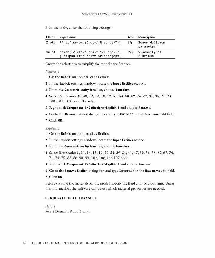
3 In the table, enter the following settings:
Create the selections to simplify the model specification.
Explicit 11 On the Definitions toolbar, click Explicit.
2 In the Explicit settings window, locate the Input Entities section.
3 From the Geometric entity level list, choose Boundary.
4 Select Boundaries 35–38, 42, 43, 48, 49, 51, 53, 68, 69, 76–79, 84, 85, 91, 93, 100, 101, 103, and 105 only.
5 Right-click Component 1>Definitions>Explicit 1 and choose Rename.
6 Go to the Rename Explicit dialog box and type Outside in the New name edit field.
7 Click OK.
Explicit 21 On the Definitions toolbar, click Explicit.
2 In the Explicit settings window, locate the Input Entities section.
3 From the Geometric entity level list, choose Boundary.
4 Select Boundaries 8, 11, 14, 15, 19, 20, 24, 29–34, 41, 47, 50, 56–58, 62, 67, 70, 71, 74, 75, 83, 86–90, 99, 102, 106, and 107 only.
5 Right-click Component 1>Definitions>Explicit 2 and choose Rename.
6 Go to the Rename Explicit dialog box and type Interior in the New name edit field.
7 Click OK.
Before creating the materials for the model, specify the fluid and solid domains. Using this information, the software can detect which material properties are needed.
C O N J U G A T E H E A T TR A N S F E R
Fluid 1Select Domains 3 and 4 only.
Name Expression Unit Description
Z_eta F*nitf.sr*exp(Q_eta/(R_const*T)) 1/s Zener-Hollomon parameter
mu_al asinh((Z_eta/A_eta)^(1/n_eta))/(3*alpha_eta*F*nitf.sr+sqrt(eps))
Pa·s Viscosity of aluminum
I D - S T R U C T U R E I N T E R A C T I O N I N A L U M I N U M E X T R U S I O N

Solved with COMSOL Multiphysics 4.4
S O L I D M E C H A N I C S
1 In the Model Builder window, under Component 1 click Solid Mechanics.
2 In the Solid Mechanics settings window, locate the Domain Selection section.
3 Click Clear Selection.
4 Select Domains 1 and 2 only.
Now, define the material for each domain.
M A T E R I A L S
On the Home toolbar, click Add Material.
A D D M A T E R I A L
1 Go to the Add Material window.
2 In the tree, select Material Library>Tool Steels>H11 mod (AISI 610)>H11 mod (AISI
610) [solid]>H11 mod (AISI 610) [solid,triple tempered].
3 In the Add Material window, click Add to Component.
M A T E R I A L S
H11 mod (AISI 610) [solid,triple tempered]1 In the Model Builder window, under Component 1>Materials click H11 mod (AISI 610)
[solid,triple tempered].
2 Select Domains 1 and 2 only.
3 In the Material settings window, locate the Material Contents section.
4 In the table, enter the following settings:
Because the heat capacity only enters the transient heat transfer equation, this setting does not affect the steady-state simulation described here; it is provided for completeness in case you will to extend the model to perform transient simulations.
Material 21 In the Model Builder window, right-click Materials and choose New Material.
2 Select Domains 3 and 4 only.
3 In the Material settings window, locate the Material Contents section.
Property Name Value Unit Property group
Heat capacity at constant pressure
Cp 4.63[N/(mm^2*K)]/rho(T[1/K])[kg/m^3]
J/(kg·K) Basic
13 | F L U I D - S T R U C T U R E I N T E R A C T I O N I N A L U M I N U M E X T R U S I O N

Solved with COMSOL Multiphysics 4.4
14 | F L U
4 In the table, enter the following settings:
5 Right-click Component 1>Materials>Material 2 and choose Rename.
6 Go to the Rename Material dialog box and type Billet in the New name edit field.
7 Click OK.
With the materials defined, you set up the remain physics of the model.
C O N J U G A T E H E A T TR A N S F E R
In the current model the viscosity in the fluid flow part is large, which implies that the model is diffusion dominated. Pseudo time stepping works poorly for this model because it is based on the scale of the convective flux.
1 In the Model Builder window’s toolbar, click the Show button and select Advanced
Physics Options in the menu.
2 In the Conjugate Heat Transfer settings window, click to expand the Advanced settings section.
3 Find the Pseudo time stepping subsection. Clear the Use pseudo time stepping for
stationary equation form check box.
Initial Values 11 In the Model Builder window, under Component 1>Conjugate Heat Transfer right-click
Fluid 1 and choose Viscous Heating.
2 In the Initial Values settings window, locate the Initial Values section.
3 In the p edit field, type P_init.
4 In the T edit field, type T_container.
Symmetry, Flow 11 On the Physics toolbar, click Boundaries and choose Symmetry, Flow.
Property Name Value Unit Property group
Density rho 2700 kg/m³ Basic
Dynamic viscosity mu mu_al Pa·s Basic
Thermal conductivity
k 210 W/(m·K) Basic
Heat capacity at constant pressure
Cp 2.94[N/(mm^2*K)]/rho J/(kg·K) Basic
Ratio of specific heats
gamma 1 1 Basic
I D - S T R U C T U R E I N T E R A C T I O N I N A L U M I N U M E X T R U S I O N

Solved with COMSOL Multiphysics 4.4
2 Select Boundaries 9 and 112 only.
Inlet 11 On the Physics toolbar, click Boundaries and choose Inlet.
2 Select Boundary 10 only.
3 In the Inlet settings window, locate the Velocity section.
4 Click the Velocity field button.
5 Specify the u0 vector as
Wall 21 On the Physics toolbar, click Boundaries and choose Wall.
2 In the Wall settings window, locate the Boundary Selection section.
3 From the Selection list, choose Outside.
4 Locate the Boundary Condition section. From the Boundary condition list, choose Slip.
Outlet 11 On the Physics toolbar, click Boundaries and choose Outlet.
2 Select Boundary 40 only.
3 In the Outlet settings window, locate the Pressure Conditions section.
4 In the p0 edit field, type P_init.
Temperature 11 On the Physics toolbar, click Boundaries and choose Temperature.
2 Select Boundaries 2, 5, and 7 only.
3 In the Temperature settings window, locate the Temperature section.
4 In the T0 edit field, type T_container.
Heat Flux 11 On the Physics toolbar, click Boundaries and choose Heat Flux.
2 Select Boundary 10 only.
3 In the Heat Flux settings window, locate the Heat Flux section.
4 Click the Inward heat flux button.
0 x
0 y
V_ram z
15 | F L U I D - S T R U C T U R E I N T E R A C T I O N I N A L U M I N U M E X T R U S I O N

Solved with COMSOL Multiphysics 4.4
16 | F L U
5 In the h edit field, type Heat_alfe.
6 In the Text edit field, type T_ram.
Heat Flux 21 On the Physics toolbar, click Boundaries and choose Heat Flux.
2 In the Heat Flux settings window, locate the Boundary Selection section.
3 From the Selection list, choose Outside.
4 Locate the Heat Flux section. Click the Inward heat flux button.
5 In the h edit field, type H_conv.
6 In the Text edit field, type T_air.
Outflow 11 On the Physics toolbar, click Boundaries and choose Outflow.
2 Select Boundary 40 only.
Thin Thermally Resistive Layer 11 On the Physics toolbar, click Boundaries and choose Thin Thermally Resistive Layer.
2 In the Thin Thermally Resistive Layer settings window, locate the Boundary Selection section.
3 From the Selection list, choose Interior.
4 Locate the Thin Thermally Resistive Layer section. In the ds edit field, type D_alfe.
5 From the ks list, choose User defined. In the associated edit field, type Heat_alfe*D_alfe.
S O L I D M E C H A N I C S
1 In the Model Builder window, under Component 1 click Solid Mechanics.
2 Select Domains 1 and 2 only.
For faster convergence use the linear elements. You can always refine the solution using the default quadratic elements.
3 In the Model Builder window’s toolbar, click the Show button and select Discretization in the menu.
4 In the Solid Mechanics settings window, click to expand the Discretization section.
5 From the Displacement field list, choose Linear.
Linear Elastic Material 1In the Model Builder window, expand the Solid Mechanics node.
I D - S T R U C T U R E I N T E R A C T I O N I N A L U M I N U M E X T R U S I O N

Solved with COMSOL Multiphysics 4.4
Thermal Expansion 11 Right-click Linear Elastic Material 1 and choose Thermal Expansion.
2 In the Thermal Expansion settings window, locate the Model Inputs section.
3 From the T list, choose Temperature.
4 Locate the Thermal Expansion Properties section. In the Tref edit field, type T_container.
Thermal Expansion 21 Right-click Linear Elastic Material 1 and choose Thermal Expansion.
2 Select Domains 2–4 only.
3 In the Thermal Expansion settings window, locate the Model Inputs section.
4 From the T list, choose Temperature.
5 Locate the Thermal Expansion Properties section. In the Tref edit field, type T_pd1.
Roller 11 On the Physics toolbar, click Boundaries and choose Roller.
2 Select Boundaries 2, 5, and 7 only.
Symmetry 11 On the Physics toolbar, click Boundaries and choose Symmetry.
2 Select Boundaries 1, 4, 110, and 111 only.
Boundary Load 11 On the Physics toolbar, click Boundaries and choose Boundary Load.
2 Select Boundaries 8, 11, 14, 15, 19, 20, 24, 29–34, 41, 47, 50, 56–58, 62, 67, 70, 71, 74, 75, 83, 86–90, 99, 102, 106, and 107 only.
3 In the Boundary Load settings window, locate the Coordinate System Selection section.
4 From the Coordinate system list, choose Boundary System 1.
5 Locate the Force section. Specify the FA vector as
0 t1
0 t2
-p n
17 | F L U I D - S T R U C T U R E I N T E R A C T I O N I N A L U M I N U M E X T R U S I O N

Solved with COMSOL Multiphysics 4.4
18 | F L U
M E S H 1
Free Triangular 11 In the Model Builder window, under Component 1 right-click Mesh 1 and choose More
Operations>Free Triangular.
2 Select Boundary 40 only.
Size 11 Right-click Component 1>Mesh 1>Free Triangular 1 and choose Size.
2 In the Size settings window, locate the Element Size section.
3 Click the Custom button.
4 Locate the Element Size Parameters section. Select the Maximum element size check box.
5 In the associated edit field, type 0.0014.
6 Select the Curvature factor check box.
7 In the associated edit field, type 0.2.
8 Click the Build Selected button.
Swept 11 In the Model Builder window, right-click Mesh 1 and choose Swept.
2 In the Swept settings window, locate the Domain Selection section.
3 From the Geometric entity level list, choose Domain.
4 Select Domain 4 only.
Distribution 11 Right-click Component 1>Mesh 1>Swept 1 and choose Distribution.
2 In the Distribution settings window, locate the Distribution section.
3 In the Number of elements edit field, type 24.
4 Click the Build All button.
Free Tetrahedral 1In the Model Builder window, right-click Mesh 1 and choose Free Tetrahedral.
Size 11 In the Model Builder window, under Component 1>Mesh 1 right-click Free Tetrahedral
1 and choose Size.
2 In the Size settings window, locate the Element Size section.
I D - S T R U C T U R E I N T E R A C T I O N I N A L U M I N U M E X T R U S I O N

Solved with COMSOL Multiphysics 4.4
3 Click the Custom button.
4 Locate the Element Size Parameters section. Select the Maximum element size check box.
5 In the associated edit field, type 0.0085.
Size 21 Right-click Free Tetrahedral 1 and choose Size.
2 In the Size settings window, locate the Geometric Entity Selection section.
3 From the Geometric entity level list, choose Boundary.
4 Select Boundaries 12 and 13 only.
5 Locate the Element Size section. Click the Custom button.
6 Locate the Element Size Parameters section. Select the Maximum element size check box.
7 In the associated edit field, type 0.002.
Size 31 Right-click Free Tetrahedral 1 and choose Size.
2 In the Size settings window, locate the Geometric Entity Selection section.
3 From the Geometric entity level list, choose Boundary.
4 Select Boundary 24 only.
5 Locate the Element Size section. Click the Custom button.
6 Locate the Element Size Parameters section. Select the Minimum element size check box.
7 In the associated edit field, type 1e-5.
Size 41 Right-click Free Tetrahedral 1 and choose Size.
2 In the Size settings window, locate the Geometric Entity Selection section.
3 From the Geometric entity level list, choose Edge.
4 Select Edges 50 and 138 only.
5 Locate the Element Size section. Click the Custom button.
6 Locate the Element Size Parameters section. Select the Minimum element size check box.
7 In the associated edit field, type 1e-5.
19 | F L U I D - S T R U C T U R E I N T E R A C T I O N I N A L U M I N U M E X T R U S I O N

Solved with COMSOL Multiphysics 4.4
20 | F L U
Size1 In the Model Builder window, under Component 1>Mesh 1 click Size.
2 In the Size settings window, locate the Element Size section.
3 From the Predefined list, choose Finer.
4 Click the Build All button.
You should now see the following meshed geometry.
S T U D Y 1
Step 1: StationaryUse two stationary study steps. Solve first for the fluid dynamics and heat transfer to determine the thermal load and the pressure load and then for the structural mechanics.
1 In the Model Builder window, expand the Study 1 node, then click Step 1: Stationary.
2 In the Stationary settings window, locate the Physics and Variables Selection section.
3 In the table, enter the following settings:
Physics Solve for Discretization
Solid Mechanics × Physics settings
I D - S T R U C T U R E I N T E R A C T I O N I N A L U M I N U M E X T R U S I O N

Solved with COMSOL Multiphysics 4.4
Step 2: Stationary 21 On the Study toolbar, click Study Steps and choose Stationary>Stationary.
2 In the Stationary settings window, locate the Physics and Variables Selection section.
3 In the table, enter the following settings:
For the structural analysis, use a memory efficient iterative solver to make it possible to solve the problem also on computers with limited memory.
Solver 11 On the Study toolbar, click Show Default Solver.
2 In the Model Builder window, expand the Study 1>Solver Configurations>Solver
1>Stationary Solver 2 node.
3 Right-click Study 1>Solver Configurations>Solver 1>Stationary Solver 2 and choose Iterative.
4 On the Home toolbar, click Compute.
R E S U L T S
Data SetsModify the first default plot to see the velocity field and streamlines at the profile section (Figure 4).
1 In the Model Builder window, under Results>Data Sets right-click Solution 2 and choose Add Selection.
2 In the Selection settings window, locate the Geometric Entity Selection section.
3 From the Geometric entity level list, choose Domain.
4 Select Domains 3 and 4 only.
Velocity1 In the Model Builder window, under Results click Velocity.
2 In the 3D Plot Group settings window, locate the Data section.
3 From the Data set list, choose Solution 2.
4 In the Model Builder window, expand the Velocity node, then click Slice 1.
5 In the Slice settings window, locate the Plane Data section.
6 From the Plane list, choose XY-planes.
Physics Solve for Discretization
Conjugate Heat Transfer × Physics settings
21 | F L U I D - S T R U C T U R E I N T E R A C T I O N I N A L U M I N U M E X T R U S I O N

Solved with COMSOL Multiphysics 4.4
22 | F L U
7 From the Entry method list, choose Coordinates.
8 In the Z-coordinates edit field, type 0.0151.
9 On the 3D Plot Group toolbar, click Plot.
10 In the Model Builder window, right-click Velocity and choose Streamline.
11 In the Streamline settings window, locate the Expression section.
12 Click Replace Expression in the upper right corner of the Expression section and select Conjugate Heat Transfer>Velocity field (Spatial). Locate the Streamline Positioning section. From the Positioning list, choose Start point controlled.
13 Locate the Coloring and Style section. From the Line type list, choose Tube.
14 Click to expand the Inherit style section. Locate the Inherit Style section. From the Plot list, choose Slice 1.
15 Right-click Results>Velocity>Streamline 1 and choose Color Expression.
16 In the Color Expression settings window, locate the Expression section.
17 Click Replace Expression in the upper right corner of the Expression section and select Conjugate Heat Transfer>Velocity magnitudein the upper-right corner of the section. On the 3D Plot Group toolbar, click Plot.
To get a better view, rotate the geometry in the Graphics window and use the Zoom
Box tool to obtain a close-up. You can preserve a view for a plot by creating a View feature node as follows:
18 In the Model Builder window’s toolbar, click the Show button and select Advanced
Results Options in the menu.
19 In the Model Builder window, expand the Results>Velocity>Streamline 1 node.
20 Right-click Results>Views and choose View 3D.
21 Use the Graphics toolbox to get a satisfying view.
22 In the Model Builder window, under Results>Views click View 3D 2.
23 In the View 3D settings window, locate the View section.
24 Select the Lock camera check box.
Next, apply the view to the velocity plot.
Velocity1 In the Model Builder window, under Results click Velocity.
2 In the 3D Plot Group settings window, locate the Plot Settings section.
3 From the View list, choose View 3D 2.
4 On the 3D Plot Group toolbar, click Plot.
I D - S T R U C T U R E I N T E R A C T I O N I N A L U M I N U M E X T R U S I O N

Solved with COMSOL Multiphysics 4.4
TemperatureThe second default plot shows the temperature (Figure 3).
1 On the 3D Plot Group toolbar, click Plot.
Stress (solid)The last plot shows the von Mises stress and deformation distribution in the container. To reproduce the Figure 5, apply the View 3D 2.
1 In the Model Builder window, under Results click Stress.
2 In the 3D Plot Group settings window, locate the Plot Settings section.
3 From the View list, choose View 3D 2.
4 On the 3D Plot Group toolbar, click Plot.
23 | F L U I D - S T R U C T U R E I N T E R A C T I O N I N A L U M I N U M E X T R U S I O N

Solved with COMSOL Multiphysics 4.4
24 | F L U
I D - S T R U C T U R E I N T E R A C T I O N I N A L U M I N U M E X T R U S I O N
Solved with COMSOL Multiphysics 4.4
F l u i d - S t r u c t u r e I n t e r a c t i o n i n a Ne two r k o f B l o od V e s s e l s
Introduction
This model studies a portion of the vascular system, in particular the upper part of the aorta (Figure 1). The aorta and its ramified blood vessels are embedded in biological tissue, specifically the cardiac muscle. The flowing blood applies pressure to the artery’s internal surfaces and its branches, thereby deforming the tissue. The analysis consists of two distinct but coupled procedures: first, a fluid-dynamics analysis including a calculation of the velocity field and pressure distribution in the blood (variable in time and in space); second, a mechanical analysis of the deformation of the tissue and artery. In this model, any change in the shape of the vessel walls does not influence the fluid domain, which implies that there is only a one-way fluid-structural coupling. However, in COMSOL Multiphysics it is possible to simulate a two-way coupling using the ALE (arbitrary Lagrangian-Eulerian) method.
Figure 1: The model domain consists of part of the aorta, its branches, and the surrounding tissue.
Model Definition
Figure 2 shows two views of the model domain, one with and one without the cardiac muscle. The model’s mechanical analysis must consider the cardiac muscle because it presents a stiffness that resists artery deformation due to the applied pressure.
1 | F L U I D - S T R U C T U R E I N T E R A C T I O N I N A N E T W O R K O F B L O O D V E S S E L S

Solved with COMSOL Multiphysics 4.4
2 | F L U
Figure 2: A view of the aorta and its ramification (branching vessels) with blood contained, shown both with (left) and without (right) the cardiac muscle.
The main characteristics of the analyses are:
• Fluid dynamics analysis
Here the model solves the Navier-Stokes equations in the blood domain. At each surface where the model brings a vessel to an abrupt end, it represents the load with a known pressure distribution.
• Mechanical analysis
Only the domains related to the biological tissues are active in this analysis. The model represents the load with the total stress distribution it computes during the fluid-dynamics analysis.
A N A L Y S I S O F R U B B E R - L I K E T I S S U E A N D A R T E R Y M A T E R I A L M O D E L S
Generally, the modeling of biological tissue is an advanced subject for several reasons:
• The material can undergo very large strains (finite deformations).
• The stress-strain relationship is generally nonlinear.
• Many hyperelastic materials are almost incompressible. You must then revise standard displacement-based finite element formulations in order to arrive at correct results (mixed formulations).
You must pay particular attention to the definition of stress and strain measures. In a geometrically nonlinear analysis the assumptions about infinitesimal displacements are no longer valid. It is necessary to consider geometrical nonlinearity in a model when:
• Significant rigid-body rotations occur (finite rotations).
I D - S T R U C T U R E I N T E R A C T I O N I N A N E T W O R K O F B L O O D V E S S E L S

Solved with COMSOL Multiphysics 4.4
• The strains are no longer small (larger than a few percent).
• The loading of the body depends on the deformation.
All of these issues are dealt with in the hyperelastic material model built-in the Nonlinear Structural Materials Module.
In this case, the displacements and strains are so small that it is sufficient to use a linear elastic material model. The material data is given for a Neo-Hookean hyperelastic material, but in the small strain limit the interpretation of the material constants is the same for a linear elastic material.
M A T E R I A L S
The model uses the following material properties:
• Blood
- density = 1060 kg/m3
- dynamic viscosity = 0.005 Ns/m2
• Artery
- density = 960 kg/m3
- Neo-Hookean hyperelastic behavior: the coefficient equals 6.20·106 N/m2, while the bulk modulus equals 20 and corresponds to a value for Poisson’s ratio, , of 0.45. An equivalent elastic modulus equals 1.0·107 N/m2.
• Cardiac muscle
- density = 1200 kg/m3
- Neo-Hookean hyperelastic behavior: the coefficient equals 7.20·106 N/m2, while the bulk modulus equals 20 and corresponds to a value for Poisson’s ratio, , of 0.45. An equivalent elastic modulus equals 1.16·106 N/m2.
F L U I D D Y N A M I C S A N A L Y S I S
The fluid dynamics analysis considers the solution of the 3D Navier-Stokes equations. You can do so in both a stationary case or in the time domain. To establish the boundary conditions, the model uses six pressure conditions with the configuration
3 | F L U I D - S T R U C T U R E I N T E R A C T I O N I N A N E T W O R K O F B L O O D V E S S E L S

Solved with COMSOL Multiphysics 4.4
4 | F L U
shown in Figure 3.
Figure 3: Boundary conditions for the fluid-flow analysis.
The pressure conditions are:
• Section 1: 11,208 Pa
• Section 2: 11,192 Pa
• Section 3: 11,148 Pa
• Section 4: 11,148 Pa
• Section 5: 11,148 Pa
• Section 6: 11,120 Pa
For the time-dependent analysis, the model uses a simple trigonometric function to vary the pressure distribution over time:
(1)
You implement this effect in COMSOL Multiphysics using Piecewise function.
1. P
2. P
3. P4. P
5. P
6. P
P = Pressure
f t
t 0 t 12---s sin
32--- 1
2--- 2 t 1
2---–
1
2---s t 3
2---s cos–
=
I D - S T R U C T U R E I N T E R A C T I O N I N A N E T W O R K O F B L O O D V E S S E L S

Solved with COMSOL Multiphysics 4.4
Results and Discussion
The flow field at the time t=1 s is displayed in Figure 4 as a slice plot.
Figure 4: Velocity field in the aorta and its ramification (branching).
Figure 5 shows the total displacement at the peak load (after 1 s). The displacements are in the order of 4 m, which suggests that the one-way multiphysics coupling is a reasonable approximation.
5 | F L U I D - S T R U C T U R E I N T E R A C T I O N I N A N E T W O R K O F B L O O D V E S S E L S

Solved with COMSOL Multiphysics 4.4
6 | F L U
Figure 5: Displacements in the blood vessel.
Notes About the COMSOL Implementation
In this model, and many other cases, an analysis which is time dependent for one physics can be treated as quasi-static from the structural mechanics point of view. You can handle this by running the structural analysis as a parametric sweep over a number of static load cases, where the time is used as the parameter. This method is used here.
Model Library path: Structural_Mechanics_Module/Bioengineering/blood_vessel
Modeling Instructions
From the File menu, choose New.
I D - S T R U C T U R E I N T E R A C T I O N I N A N E T W O R K O F B L O O D V E S S E L S

Solved with COMSOL Multiphysics 4.4
N E W
1 In the New window, click the Model Wizard button.
M O D E L W I Z A R D
1 In the Model Wizard window, click the 3D button.
2 In the Select physics tree, select Fluid Flow>Single-Phase Flow>Laminar Flow (spf).
3 Click the Add button.
4 In the Select physics tree, select Structural Mechanics>Solid Mechanics (solid).
5 Click the Add button.
6 Click the Study button.
7 In the tree, select Preset Studies for Selected Physics>Time Dependent.
8 Click the Done button.
G L O B A L D E F I N I T I O N S
Parameters1 On the Home toolbar, click Parameters.
2 In the Parameters settings window, locate the Parameters section.
3 In the table, enter the following settings:
Piecewise 11 On the Home toolbar, click Functions and choose Global>Piecewise.
2 In the Piecewise settings window, locate the Function Name section.
3 In the Function name edit field, type f.
4 Locate the Definition section. Find the Intervals subsection. In the Argument edit field, type t.
5 In the table, enter the following settings:
6 Locate the Units section. In the Arguments edit field, type s.
Name Expression Value Description
t 0 0 Time continuation parameter
Start End Function
0 0.5 sin(pi*t)
0.5 1 1.5-0.5*cos(-2*pi*(0.5-t))
7 | F L U I D - S T R U C T U R E I N T E R A C T I O N I N A N E T W O R K O F B L O O D V E S S E L S

Solved with COMSOL Multiphysics 4.4
8 | F L U
7 In the Function edit field, type 1.
8 Click the Plot button.
G E O M E T R Y 1
The geometry for this model is available as an MPHBIN-file. Import this file as follows.
Import 11 On the Home toolbar, click Import.
2 In the Import settings window, locate the Import section.
3 Click the Browse button.
4 Browse to the model’s Model Library folder and double-click the file blood_vessel.mphbin.
5 Click the Import button.
The length unit in the imported geometry is centimeters, while the default length unit in COMSOL Multiphysics is meters. Therefore, you need to rescale the geometry.
Scale 11 On the Geometry toolbar, click Scale.
2 In the Scale settings window, locate the Scale Factor section.
3 In the Factor edit field, type 0.01.
4 Select the object imp1 only.
5 Click the Build Selected button.
6 Click the Go to Default 3D View button on the Graphics toolbar.
Form Union1 In the Model Builder window, under Component 1>Geometry 1 right-click Form Union
and choose Build Selected.
I D - S T R U C T U R E I N T E R A C T I O N I N A N E T W O R K O F B L O O D V E S S E L S

Solved with COMSOL Multiphysics 4.4
2 Click the Transparency button on the Graphics toolbar to see the interior.
D E F I N I T I O N S
Next, define a number of selections as sets of geometric entities for use in setting up the model.
3 Explicit 1
1 On the Definitions toolbar, click Explicit.
2 Select Domain 3 only.
3 Right-click Component 1>Definitions>Explicit 1 and choose Rename.
4 Go to the Rename Explicit dialog box and type Blood in the New name edit field.
5 Click OK.
Explicit 21 On the Definitions toolbar, click Explicit.
2 Select Domain 2 only.
3 Right-click Component 1>Definitions>Explicit 2 and choose Rename.
4 Go to the Rename Explicit dialog box and type Artery in the New name edit field.
5 Click OK.
9 | F L U I D - S T R U C T U R E I N T E R A C T I O N I N A N E T W O R K O F B L O O D V E S S E L S

Solved with COMSOL Multiphysics 4.4
10 | F L U
Explicit 31 On the Definitions toolbar, click Explicit.
2 Select Domain 1 only.
3 Right-click Component 1>Definitions>Explicit 3 and choose Rename.
4 Go to the Rename Explicit dialog box and type Muscle in the New name edit field.
5 Click OK.
Explicit 41 On the Definitions toolbar, click Explicit.
2 In the Explicit settings window, locate the Input Entities section.
3 From the Geometric entity level list, choose Boundary.
4 Click Paste Selection.
5 Go to the Paste Selection dialog box.
6 In the Selection edit field, type 38.
7 Click the OK button.
8 Right-click Component 1>Definitions>Explicit 4 and choose Rename.
9 Go to the Rename Explicit dialog box and type Inlet in the New name edit field.
10 Click OK.
Explicit 51 On the Definitions toolbar, click Explicit.
2 In the Explicit settings window, locate the Input Entities section.
3 From the Geometric entity level list, choose Boundary.
4 Select Boundary 19 only.
5 Right-click Component 1>Definitions>Explicit 5 and choose Rename.
6 Go to the Rename Explicit dialog box and type Outlet 1 in the New name edit field.
7 Click OK.
Explicit 61 On the Definitions toolbar, click Explicit.
2 In the Explicit settings window, locate the Input Entities section.
3 From the Geometric entity level list, choose Boundary.
4 Select Boundary 9 only.
5 Right-click Component 1>Definitions>Explicit 6 and choose Rename.
I D - S T R U C T U R E I N T E R A C T I O N I N A N E T W O R K O F B L O O D V E S S E L S

Solved with COMSOL Multiphysics 4.4
6 Go to the Rename Explicit dialog box and type Outlet 2 in the New name edit field.
7 Click OK.
Explicit 71 On the Definitions toolbar, click Explicit.
2 In the Explicit settings window, locate the Input Entities section.
3 From the Geometric entity level list, choose Boundary.
4 Select Boundary 41 only.
5 Right-click Component 1>Definitions>Explicit 7 and choose Rename.
6 Go to the Rename Explicit dialog box and type Outlet 3 in the New name edit field.
7 Click OK.
Explicit 81 On the Definitions toolbar, click Explicit.
2 In the Explicit settings window, locate the Input Entities section.
3 From the Geometric entity level list, choose Boundary.
4 Select Boundary 70 only.
5 Right-click Component 1>Definitions>Explicit 8 and choose Rename.
6 Go to the Rename Explicit dialog box and type Outlet 4 in the New name edit field.
7 Click OK.
Explicit 91 On the Definitions toolbar, click Explicit.
2 In the Explicit settings window, locate the Input Entities section.
3 From the Geometric entity level list, choose Boundary.
4 Select Boundary 86 only.
5 Right-click Component 1>Definitions>Explicit 9 and choose Rename.
6 Go to the Rename Explicit dialog box and type Outlet 5 in the New name edit field.
7 Click OK.
Explicit 101 On the Definitions toolbar, click Explicit.
2 In the Explicit settings window, locate the Input Entities section.
3 From the Geometric entity level list, choose Boundary.
4 Select Boundaries 1–6, 12, 26, 27, 30, 33, 64, 67, 85, and 87 only.
11 | F L U I D - S T R U C T U R E I N T E R A C T I O N I N A N E T W O R K O F B L O O D V E S S E L S

Solved with COMSOL Multiphysics 4.4
12 | F L U
5 Right-click Component 1>Definitions>Explicit 10 and choose Rename.
6 Go to the Rename Explicit dialog box and type Roller boundaries in the New name edit field.
7 Click OK.
The roller boundaries are the free boundaries of muscle and artery that are neither in contact with each other nor with blood.
Explicit 111 On the Definitions toolbar, click Explicit.
2 In the Explicit settings window, locate the Input Entities section.
3 From the Geometric entity level list, choose Boundary.
4 Select the All boundaries check box.
5 Select Boundaries 10, 11, 16, 17, 20, 21, 23, 24, 36, 37, 39, 40, 42, 43, 45, 46, 50–53, 58, 59, 61, 62, 68, 69, 71, 72, 75, 76, 79, 80, 82, and 83 only.
6 Right-click Component 1>Definitions>Explicit 11 and choose Rename.
7 Go to the Rename Explicit dialog box and type Loaded boundaries in the New name edit field.
8 Click OK.
The loaded boundaries are the inner artery boundaries that are in contact with blood.
Explicit 121 On the Definitions toolbar, click Explicit.
2 Select Domain 2 only.
3 In the Explicit settings window, locate the Output Entities section.
4 From the Output entities list, choose Adjacent boundaries.
5 Select the Interior boundaries check box.
6 Right-click Component 1>Definitions>Explicit 12 and choose Rename.
7 Go to the Rename Explicit dialog box and type Artery walls in the New name edit field.
8 Click OK.
L A M I N A R F L O W
1 In the Laminar Flow settings window, locate the Domain Selection section.
2 From the Selection list, choose Blood.
I D - S T R U C T U R E I N T E R A C T I O N I N A N E T W O R K O F B L O O D V E S S E L S

Solved with COMSOL Multiphysics 4.4
3 Locate the Physical Model section. From the Compressibility list, choose Incompressible flow.
Inlet 11 On the Physics toolbar, click Boundaries and choose Inlet.
2 In the Inlet settings window, locate the Boundary Selection section.
3 From the Selection list, choose Inlet.
4 Locate the Boundary Condition section. From the Boundary condition list, choose Pressure, no viscous stress.
5 Locate the Pressure, No Viscous Stress section. In the p0 edit field, type 11208[Pa]*f(t).
Outlet 11 On the Physics toolbar, click Boundaries and choose Outlet.
2 In the Outlet settings window, locate the Boundary Selection section.
3 From the Selection list, choose Outlet 1.
4 Locate the Pressure Conditions section. In the p0 edit field, type 11192[Pa]*f(t).
Outlet 21 On the Physics toolbar, click Boundaries and choose Outlet.
2 In the Outlet settings window, locate the Boundary Selection section.
3 From the Selection list, choose Outlet 2.
4 Locate the Pressure Conditions section. In the p0 edit field, type 11148[Pa]*f(t).
Outlet 31 On the Physics toolbar, click Boundaries and choose Outlet.
2 In the Outlet settings window, locate the Boundary Selection section.
3 From the Selection list, choose Outlet 3.
4 Locate the Pressure Conditions section. In the p0 edit field, type 11148[Pa]*f(t).
Outlet 41 On the Physics toolbar, click Boundaries and choose Outlet.
2 In the Outlet settings window, locate the Boundary Selection section.
3 From the Selection list, choose Outlet 4.
4 Locate the Pressure Conditions section. In the p0 edit field, type 11148[Pa]*f(t).
13 | F L U I D - S T R U C T U R E I N T E R A C T I O N I N A N E T W O R K O F B L O O D V E S S E L S

Solved with COMSOL Multiphysics 4.4
14 | F L U
Outlet 51 On the Physics toolbar, click Boundaries and choose Outlet.
2 In the Outlet settings window, locate the Boundary Selection section.
3 From the Selection list, choose Outlet 5.
4 Locate the Pressure Conditions section. In the p0 edit field, type 11120[Pa]*f(t).
S O L I D M E C H A N I C S
1 In the Model Builder window, under Component 1 click Solid Mechanics.
2 Select Domains 1 and 2 only.
3 In the Model Builder window’s toolbar, click the Show button and select Discretization in the menu.
4 In the Solid Mechanics settings window, click to expand the Discretization section.
5 From the Displacement field list, choose Linear.
This is just to keep down the size of the model.
Linear Elastic Material 11 In the Model Builder window, under Component 1>Solid Mechanics click Linear Elastic
Material 1.
2 In the Linear Elastic Material settings window, locate the Linear Elastic Material section.
3 From the Specify list, choose Lamé parameters.
Roller 11 On the Physics toolbar, click Boundaries and choose Roller.
2 In the Roller settings window, locate the Boundary Selection section.
3 From the Selection list, choose Roller boundaries.
Boundary Load 11 On the Physics toolbar, click Boundaries and choose Boundary Load.
The laminar flow physics interface defines variables for the total stress applied to the fluid at the wall (spf.T_stressx, spf.T_stressy, and spf.T_stressz). You can use these variables to define the fluid forces applied to the blood vessel wall.
2 In the Boundary Load settings window, locate the Boundary Selection section.
3 From the Selection list, choose Loaded boundaries.
I D - S T R U C T U R E I N T E R A C T I O N I N A N E T W O R K O F B L O O D V E S S E L S
Solved with COMSOL Multiphysics 4.4
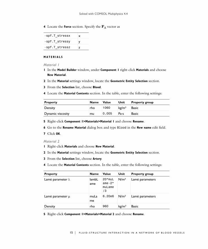
4 Locate the Force section. Specify the FA vector as
M A T E R I A L S
Material 11 In the Model Builder window, under Component 1 right-click Materials and choose
New Material.
2 In the Material settings window, locate the Geometric Entity Selection section.
3 From the Selection list, choose Blood.
4 Locate the Material Contents section. In the table, enter the following settings:
5 Right-click Component 1>Materials>Material 1 and choose Rename.
6 Go to the Rename Material dialog box and type Blood in the New name edit field.
7 Click OK.
Material 21 Right-click Materials and choose New Material.
2 In the Material settings window, locate the Geometric Entity Selection section.
3 From the Selection list, choose Artery.
4 Locate the Material Contents section. In the table, enter the following settings:
5 Right-click Component 1>Materials>Material 2 and choose Rename.
-spf.T_stressx x
-spf.T_stressy y
-spf.T_stressz z
Property Name Value Unit Property group
Density rho 1060 kg/m³ Basic
Dynamic viscosity mu 0.005 Pa·s Basic
Property Name Value Unit Property group
Lamé parameter lambLame
20*muLame-2*muLame/3
N/m² Lamé parameters
Lamé parameter muLame
6.20e6 N/m² Lamé parameters
Density rho 960 kg/m³ Basic
15 | F L U I D - S T R U C T U R E I N T E R A C T I O N I N A N E T W O R K O F B L O O D V E S S E L S

Solved with COMSOL Multiphysics 4.4
16 | F L U
6 Go to the Rename Material dialog box and type Artery in the New name edit field.
7 Click OK.
Material 31 Right-click Materials and choose New Material.
2 In the Material settings window, locate the Geometric Entity Selection section.
3 From the Selection list, choose Muscle.
4 Locate the Material Contents section. In the table, enter the following settings:
5 Right-click Component 1>Materials>Material 3 and choose Rename.
6 Go to the Rename Material dialog box and type Muscle in the New name edit field.
7 Click OK.
M E S H 1
Free Tetrahedral 1In the Model Builder window, under Component 1 right-click Mesh 1 and choose Free Tetrahedral.
Size 11 In the Model Builder window, under Component 1>Mesh 1 right-click Free Tetrahedral
1 and choose Size.
2 In the Size settings window, locate the Geometric Entity Selection section.
3 From the Geometric entity level list, choose Domain.
4 From the Selection list, choose Blood.
5 Locate the Element Size section. Click the Custom button.
6 Locate the Element Size Parameters section. Select the Maximum element size check box.
7 In the associated edit field, type 1e-3.
Property Name Value Unit Property group
Lamé parameter lambLame
20*muLame-2*muLame/3
N/m² Lamé parameters
Lamé parameter muLame
7.20e6 N/m² Lamé parameters
Density rho 1200 kg/m³ Basic
I D - S T R U C T U R E I N T E R A C T I O N I N A N E T W O R K O F B L O O D V E S S E L S

Solved with COMSOL Multiphysics 4.4
Size1 In the Model Builder window, under Component 1>Mesh 1 click Size.
2 In the Size settings window, locate the Element Size section.
3 From the Predefined list, choose Fine.
4 Click the Build All button.
S T U D Y 1
The structural problem is quasi-static, so you can use the time just as a parameter for the parametric solver, together with a stationary solver. Thus the whole study can be divided into two steps. First run the transient study for the fluid-mechanics part of the problem and then use the stationary solver to solve the structural part using the solution from first transient study.
Step 1: Time Dependent1 In the Model Builder window, expand the Study 1 node, then click Step 1: Time
Dependent.
2 In the Time Dependent settings window, locate the Study Settings section.
3 In the Times edit field, type range(0,0.05,1).
17 | F L U I D - S T R U C T U R E I N T E R A C T I O N I N A N E T W O R K O F B L O O D V E S S E L S

Solved with COMSOL Multiphysics 4.4
18 | F L U
4 Locate the Physics and Variables Selection section. In the table, enter the following settings:
Step 2: Stationary1 On the Study toolbar, click Study Steps and choose Stationary>Stationary.
2 In the Stationary settings window, locate the Physics and Variables Selection section.
3 In the table, enter the following settings:
4 Click to expand the Study extensions section. Locate the Study Extensions section. Select the Auxiliary sweep check box.
5 Click Add.
6 In the table, enter the following settings:
7 Click to expand the Values of dependent variables section. Locate the Values of
Dependent Variables section. Select the Values of variables not solved for check box.
8 From the Method list, choose Solution.
9 From the Study list, choose Study 1, Time Dependent.
10 From the Selection list, choose All.
11 On the Home toolbar, click Compute.
R E S U L T S
Velocity (spf)12 Click the Transparency button on the Graphics toolbar to restore the original
transparency state.
R E S U L T S
By default, you get a slice plot of the velocity and a contour plot of the fluid pressure on the wall surface.The plot in Figure 4 corresponds to the first default plot.
Physics Solve for Discretization
Solid Mechanics × physics
Physics Solve for Discretization
Laminar Flow × physics
Auxiliary parameter Parameter value list
t range(0,0.05,1)
I D - S T R U C T U R E I N T E R A C T I O N I N A N E T W O R K O F B L O O D V E S S E L S

Solved with COMSOL Multiphysics 4.4
1 In the Model Builder window, expand the Velocity (spf) node, then click Slice 1.
2 In the Slice settings window, locate the Plane Data section.
3 From the Plane list, choose ZX-planes.
4 In the Planes edit field, type 1.
5 On the Velocity (spf) toolbar, click Plot.
6 Click the Go to Default 3D View button on the Graphics toolbar.
To reproduce the plot shown in Figure 5, begin by defining a selection for the solution data set to make interior boundaries visible in the plot.
Data Sets1 On the Results toolbar, click More Data Sets and choose Solution.
2 In the Model Builder window, under Results>Data Sets right-click Solution 2 and choose Add Selection.
3 In the Selection settings window, locate the Geometric Entity Selection section.
4 From the Geometric entity level list, choose Boundary.
5 From the Selection list, choose Artery walls.
Stress (solid)1 In the Model Builder window, under Results click Stress (solid).
2 In the 3D Plot Group settings window, locate the Data section.
3 From the Data set list, choose Solution 2.
4 Right-click Results>Stress (solid) and choose Rename.
5 Go to the Rename 3D Plot Group dialog box and type Displacement (solid) in the New name edit field.
6 Click OK.
Displacement (solid)1 In the Model Builder window, expand the Results>Displacement (solid) node, then
click Surface 1.
2 In the Surface settings window, click Replace Expression in the upper-right corner of the Expression section. From the menu, choose Solid Mechanics>Displacement>Total
displacement (solid.disp).
3 Locate the Expression section. From the Unit list, choose µm.
4 In the Model Builder window, expand the Results>Displacement (solid)>Surface 1 node, then click Deformation.
19 | F L U I D - S T R U C T U R E I N T E R A C T I O N I N A N E T W O R K O F B L O O D V E S S E L S

Solved with COMSOL Multiphysics 4.4
20 | F L U
5 In the Deformation settings window, locate the Scale section.
6 Select the Scale factor check box.
7 In the associated edit field, type 300.
8 In the Model Builder window, click Displacement (solid).
9 In the 3D Plot Group settings window, click to expand the Title section.
10 From the Title type list, choose Manual.
11 In the Title text area, type Time=1 Surface: Total displacement (m) Surface
Deformation: Displacement field.
12 On the Displacement (solid) toolbar, click Plot.
13 Click the Go to Default 3D View button on the Graphics toolbar.
14 Click the Zoom Extents button on the Graphics toolbar.
I D - S T R U C T U R E I N T E R A C T I O N I N A N E T W O R K O F B L O O D V E S S E L S

Solved with COMSOL Multiphysics 4.4
B r a c k e t Geome t r y
This is a template MPH-file containing the bracket geometry. For a description of this model, including detailed step-by-step instructions showing how to build it, see the section “The Fundamentals: A Static Linear Analysis” in the book Introduction to the Structural Mechanics Module.
Model Library path: Structural_Mechanics_Module/Tutorial_Models/bracket_basic
1 | B R A C K E T G E O M E T R Y

Solved with COMSOL Multiphysics 4.4
2 | B R A
C K E T G E O M E T R Y
Solved with COMSOL Multiphysics 4.4
B r a c k e t—Con t a c t
Introduction
This example illustrates how to solve a structural contact problem between two elastic bodies. You will learn how to manually add a Contact pair node and define the boundaries to be in contact, then add the contact pair boundary condition to enable the structural contact between the two parts of the assembly.
It is recommended you review the Introduction to the Structural Mechanics Module, which includes background information and discusses the bracket_basic.mph model relevant to this example.
Model Definition
This model is an extension to the model example described in the section “The Fundamentals: A Static Linear Analysis” in the Introduction to the Structural Mechanics Module. In this model, a prescribed expression is used to represent the load applied to the bracket hole while in the current model a pin is added (see Figure 1). A load is applied to the pin and the contact pressure between the pin and the bracket is computed.
1 | B R A C K E T — C O N T A C T

Solved with COMSOL Multiphysics 4.4
2 | B R A
Figure 1: The geometry of the bracket and the pin.
Results and Discussion
Figure 2 shows the Von Mises stress distribution in both the bracket and pin geometry.
C K E T — C O N T A C T

Solved with COMSOL Multiphysics 4.4
Figure 2: Von Mises stress distribution, where the stress concentration is in the contact region.
Figure 3 shows the contact pressure distribution on the destination contact boundary.
Figure 3: Contact pressure distribution along the destination contact boundary.
3 | B R A C K E T — C O N T A C T

Solved with COMSOL Multiphysics 4.4
4 | B R A
Notes About the COMSOL Implementation
In COMSOL Multiphysics the contact pressure is evaluated as a function of the gap distance between the parts that are set to be in contact. This gap value is evaluated in the Contact pair node, where you define the source and destination boundaries.
When modeling contact it is recommended to set a finer mesh on the destination contact boundary compare to the source contact boundary.
When modeling a frictionless contact, it is important to sufficiently constrain the displacements on both parts of the assembly. In this example, you use a spring foundation feature to constrain the pin movement in y- and z-directions.
In addition, you set an initial overlap of the parts to stabilize the initial iteration in the contact computations.
Read more about how to set contact problem in the Introduction to Contact Modeling in the Structural Mechanics User’s Guide.
Model Library path: Structural_Mechanics_Module/Tutorial_Models/bracket_contact
Modeling Instructions
1 On the Home toolbar, click Model Library.
2 Go to the Model Library window. In the Model Library tree, select Structural Mechanics
Module>Tutorial Models>bracket basic.
3 Click Open Model.
C O M P O N E N T 1
On the Home toolbar, click Add Physics.
A D D P H Y S I C S
1 Go to the Add Physics window.
2 In the Add physics tree, select Structural Mechanics>Solid Mechanics (solid).
3 In the Add physics window, click Add to Component.
C K E T — C O N T A C T

Solved with COMSOL Multiphysics 4.4
R O O T
On the Home toolbar, click Add Study.
A D D S T U D Y
1 Go to the Add Study window.
2 Find the Studies subsection. In the tree, select Preset Studies>Stationary.
3 In the Add study window, click Add Study.
G E O M E T R Y 1
Import 1 (imp1)1 In the Model Builder window, under Component 1 >Geometry 1 click Import 1.
2 In the Import settings window, locate the Import section.
3 Click the Browse button.
4 Browse to the model’s Model Library folder and double-click the file bracket_symmetry.mphbin.
5 Click the Import button.
Cylinder 1 (cyl1)1 On the Geometry toolbar, click Cylinder.
2 In the Cylinder settings window, locate the Size and Shape section.
3 In the Radius edit field, type 24[mm].
4 In the Height edit field, type 16[mm].
5 Locate the Position section. In the x edit field, type -4[mm].
To improve the convergence, create the assembly geometry with an initial overlap of the parts.
6 In the y edit field, type y0-0.8[mm].
7 In the z edit field, type z0-0.8[mm].
8 Locate the Axis section. From the Axis type list, choose Cartesian.
9 In the x edit field, type 1.
10 In the z edit field, type 0.
Form Union (fin)1 In the Model Builder window, under Component 1>Geometry 1 click Form Union.
2 In the Form Union/Assembly settings window, locate the Form Union/Assembly section.
3 From the Action list, choose Form an assembly.
5 | B R A C K E T — C O N T A C T

Solved with COMSOL Multiphysics 4.4
6 | B R A
4 Clear the Create pairs check box.
5 Click the Build Selected button.
6 Click the Zoom Extents button on the Graphics toolbar.
D E F I N I T I O N S
You will now specify the boundaries to be in contact using a contact pair feature node.
1 On the Definitions toolbar, click Pairs and choose Contact Pair.
2 Select Boundary 2 only.
3 In the Pair settings window, locate the Destination Boundaries section.
4 Select the Active toggle button.
5 Select Boundary 8 only.
S O L I D M E C H A N I C S
Contact 11 On the Physics toolbar, click Pairs and choose Contact.
2 In the Contact settings window, locate the Pair Selection section.
3 In the Pairs list, select Contact Pair 1.
Fixed Constraint 11 On the Physics toolbar, click Domains and choose Fixed Constraint.
2 In the Fixed Constraint settings window, locate the Domain Selection section.
3 From the Selection list, choose Box 1.
Symmetry 11 On the Physics toolbar, click Boundaries and choose Symmetry.
2 Select Boundaries 49 and 50 only.
Roller 11 On the Physics toolbar, click Boundaries and choose Roller.
2 Select Boundary 6 only.
Boundary Load 11 On the Physics toolbar, click Boundaries and choose Boundary Load.
2 In the Boundary Load settings window, locate the Boundary Selection section.
3 Click Paste Selection.
4 Go to the Paste Selection dialog box.
C K E T — C O N T A C T

Solved with COMSOL Multiphysics 4.4
5 In the Selection edit field, type 1.
6 Click the OK button.
7 In the Boundary Load settings window, locate the Force section.
8 From the Load type list, choose Total force.
9 Specify the Ftot vector as
The expected pin displacement is of order 0.1 mm. You use the total spring constant of 5 N/mm, which will result into an extra force negligible compared to the applied load.
Spring Foundation 11 On the Physics toolbar, click Domains and choose Spring Foundation.
2 Select Domain 1 only.
3 In the Spring Foundation settings window, locate the Spring section.
4 From the Spring type list, choose Total spring constant.
5 Specify the ktot vector as
M E S H 1
Free Tetrahedral 1In the Model Builder window, under Component 1 right-click Mesh 1 and choose Free Tetrahedral.
Size 11 In the Model Builder window, under Component 1 >Mesh 1 right-click Free Tetrahedral
1 and choose Size.
Set a finer mesh on the contact destination boundary compared to the contact source boundary.
2 In the Size settings window, locate the Geometric Entity Selection section.
0 x
-5e3 y
-5e3 z
0 x
5[N/mm] y
5[N/mm] z
7 | B R A C K E T — C O N T A C T

Solved with COMSOL Multiphysics 4.4
8 | B R A
3 From the Geometric entity level list, choose Boundary.
4 Select Boundary 8 only.
5 Locate the Element Size section. Click the Custom button.
6 Locate the Element Size Parameters section. Select the Maximum element size check box.
7 In the associated edit field, type 3[mm].
Size 21 Right-click Free Tetrahedral 1 and choose Size.
2 In the Size settings window, locate the Geometric Entity Selection section.
3 From the Geometric entity level list, choose Boundary.
4 Select Boundary 2 only.
5 Locate the Element Size section. Click the Custom button.
6 Locate the Element Size Parameters section. Select the Maximum element size check box.
7 In the associated edit field, type 4[mm].
8 Click the Build All button.
S T U D Y 1
Solver 11 On the Study toolbar, click Show Default Solver.
2 In the Model Builder window, expand the Study 1>Solver Configurations>Solver
1>Dependent Variables 1 node, then click Displacement field (Material) (comp1.u).
3 In the Field settings window, locate the Scaling section.
4 In the Scale edit field, type 1e-4.
5 On the Home toolbar, click Compute.
R E S U L T S
Stress (solid)Click the Go to Default 3D View button on the Graphics toolbar.
Data Sets1 On the Results toolbar, click More Data Sets and choose Surface.
2 Select Boundary 8 only.
C K E T — C O N T A C T

Solved with COMSOL Multiphysics 4.4
2D Plot Group 21 On the Home toolbar, click Add Plot Group and choose 2D Plot Group.
2 In the Model Builder window, under Results right-click 2D Plot Group 2 and choose Surface.
3 In the Surface settings window, click Replace Expression in the upper-right corner of the Expression section. From the menu choose Solid Mechanics>Contact pressure,
contact pair p1 (solid.Tn_p1).
4 On the 2D plot group 2 toolbar, click Plot.
9 | B R A C K E T — C O N T A C T

Solved with COMSOL Multiphysics 4.4
10 | B R
A C K E T — C O N T A C T
Solved with COMSOL Multiphysics 4.4
B r a c k e t—Eig en f r e qu en c y
Introduction
In this example you will learn how to perform an eigenfrequency analysis for both an unloaded structure and a prestressed structure.
In the case when the structure is subjected to a constant external load, the stiffness generated by the stress may affect the natural frequencies of the structure. Tensile stresses tend to increase the natural frequencies, while compressive stresses tend to decrease them.
It is recommended you review the Introduction to the Structural Mechanics Module, which includes background information and discusses the bracket_basic.mph model relevant to this example.
Model Definition
This model is an extension to the model example described in the section “The Fundamentals: A Static Linear Analysis” in the Introduction to the Structural Mechanics Module.
1 | B R A C K E T — E I G E N F R E Q U E N C Y
Solved with COMSOL Multiphysics 4.4
2 | B R A
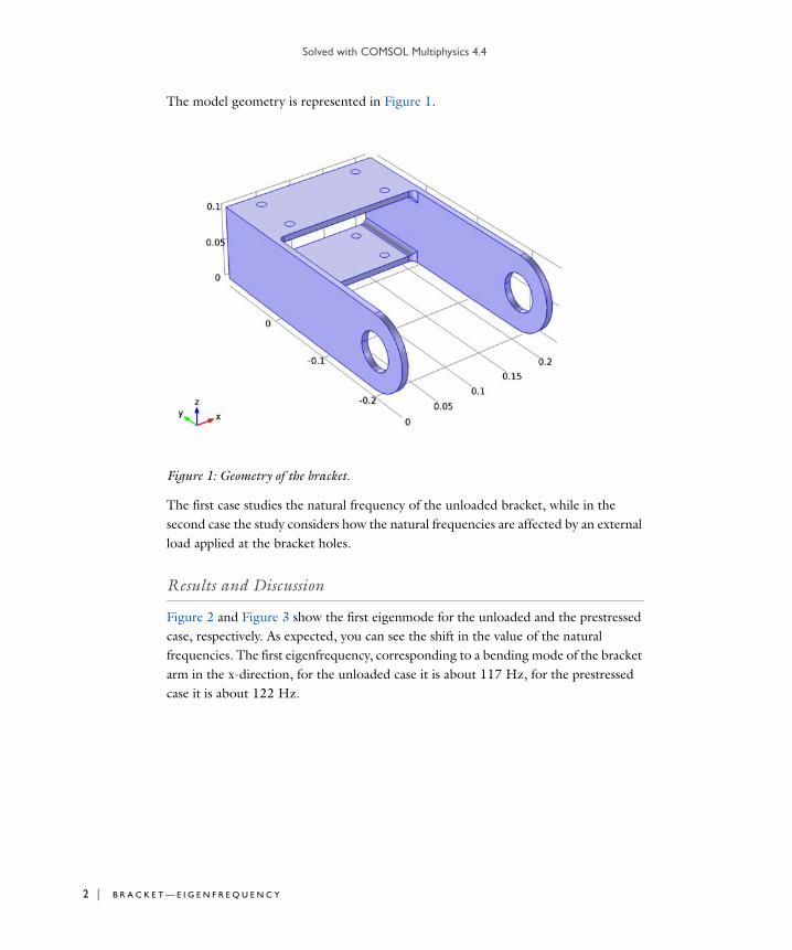
The model geometry is represented in Figure 1.
Figure 1: Geometry of the bracket.
The first case studies the natural frequency of the unloaded bracket, while in the second case the study considers how the natural frequencies are affected by an external load applied at the bracket holes.
Results and Discussion
Figure 2 and Figure 3 show the first eigenmode for the unloaded and the prestressed case, respectively. As expected, you can see the shift in the value of the natural frequencies. The first eigenfrequency, corresponding to a bending mode of the bracket arm in the x-direction, for the unloaded case it is about 117 Hz, for the prestressed case it is about 122 Hz.
C K E T — E I G E N F R E Q U E N C Y

Solved with COMSOL Multiphysics 4.4
Figure 2: First eigenmode for the unloaded case.
Figure 3: First eigenmode for the prestressed case.
3 | B R A C K E T — E I G E N F R E Q U E N C Y

Solved with COMSOL Multiphysics 4.4
4 | B R A
Notes About the COMSOL Implementation
For a structural mechanics application in COMSOL Multiphysics, there are two predefined study types available for eigenfrequency analysis: Eigenfrequency and Prestressed Analysis, Eigenfrequency.
The eigenfrequency analysis compute the natural frequencies of the unloaded structure. The contribution of any load boundary condition is disregarded and the Prescribed displacement constraints are considered as having the value zero.
The prestressed eigenfrequency analysis, however first performs a stationary analysis to take into account the different loads and non-zero displacement constraints. The stress is then added automatically to the stiffness used in the eigenfrequency calculation.
Model Library path: Structural_Mechanics_Module/Tutorial_Models/bracket_eigenfrequency
Modeling Instructions
1 On the Home toolbar, click Model Library.
2 Go to the Model Library window. In the Model Library tree, select Structural Mechanics
Module>Tutorial Models>bracket basic.
3 Click Open Model.
C O M P O N E N T 1
1 On the Home toolbar, click Add Physics.
A D D P H Y S I C S
1 Go to the Add Physics window.
2 In the Add physics tree, select Structural Mechanics>Solid Mechanics.
3 In the Add physics window, click Add to Component.
R O O T
On the Home toolbar, click Add Study.
A D D S T U D Y
1 Go to the Add Study window.
C K E T — E I G E N F R E Q U E N C Y
Solved with COMSOL Multiphysics 4.4
2 Find the Studies subsection. In the tree, select Preset Studies>Eigenfrequency.
3 In the Add study window, click Add Study.
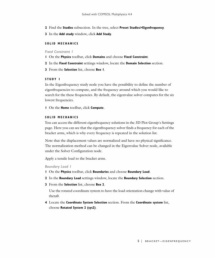
S O L I D M E C H A N I C S
Fixed Constraint 11 On the Physics toolbar, click Domains and choose Fixed Constraint.
2 In the Fixed Constraint settings window, locate the Domain Selection section.
3 From the Selection list, choose Box 1.
S T U D Y 1
In the Eigenfrequency study node you have the possibility to define the number of eigenfrequencies to compute, and the frequency around which you would like to search for the these frequencies. By default, the eigenvalue solver computes for the six lowest frequencies.
1 On the Home toolbar, click Compute.
S O L I D M E C H A N I C S
You can access the different eigenfrequency solutions in the 3D Plot Group's Settings page. Here you can see that the eigenfrequency solver finds a frequency for each of the bracket arms, which is why every frequency is repeated in the solution list.
Note that the displacement values are normalized and have no physical significance. The normalization method can be changed in the Eigenvalue Solver node, available under the Solver Configuration node.
Apply a tensile load to the bracket arms.
Boundary Load 11 On the Physics toolbar, click Boundaries and choose Boundary Load.
2 In the Boundary Load settings window, locate the Boundary Selection section.
3 From the Selection list, choose Box 2.
Use the rotated coordinate system to have the load orientation change with value of theta0.
4 Locate the Coordinate System Selection section. From the Coordinate system list, choose Rotated System 2 (sys2).
5 | B R A C K E T — E I G E N F R E Q U E N C Y

Solved with COMSOL Multiphysics 4.4
6 | B R A
5 Locate the Force section. Specify the FA vector as
A D D S T U D Y
The prestressed eigenfrequency analysis is available as a predefined study.
1 Go to the Add Study window.
2 Find the Studies subsection. In the tree, select Preset Studies>Prestressed Analysis,
Eigenfrequency.
3 In the Add study window, click Add Study.
S T U D Y 2
Step 1: StationaryThe newly generated study combines one stationary analysis and one eigenfrequency analysis.
1 On the Home toolbar, click Compute.
R E S U L T S
Mode Shape (solid) 11 Click the Zoom Extents button on the Graphics toolbar.
In the Settings page of the second plot group you can see the list of the new eigenfrequencies.
0 x1
loadIntensity x2
0 x3
C K E T — E I G E N F R E Q U E N C Y

Solved with COMSOL Multiphysics 4.4
B r a c k e t—Frequ en c y Doma i n Ana l y s i s
Introduction
The frequency response analysis solves for the linear steady-state response of a structure from harmonic loads. The problem is solved in the frequency domain and you can set a range of frequencies at which to compute the structural displacements.
In this example you will see how to perform a frequency response analysis of a structure under harmonic load but also how to perform a frequency response analysis of a prestressed structure.
It is recommended you review the Introduction to the Structural Mechanics Module, which includes background information and discusses the bracket_basic.mph model relevant to this example.
Model Definition
This model is an extension to the model example described in the section “The Fundamentals: A Static Linear Analysis” in the Introduction to the Structural Mechanics Module.
The model geometry is represented in Figure 1.
1 | B R A C K E T — F R E Q U E N C Y D O M A I N A N A L Y S I S

Solved with COMSOL Multiphysics 4.4
2 | B R A
Figure 1: Bracket geometry
You will study two load cases, the first one consists of a fully harmonic load case with an external load of 100 kPa applied to the bracket arms, the second load case consists of a combination of a static load and a harmonic perturbation.
An eigenfrequency analysis of this problem is performed in the model Bracket—Eigenfrequency. This model shows that the first resonance frequency is 117 Hz. For the loaded case, the eigenfrequency solver shows that the first resonance frequency is about 122 Hz. In order to capture the resonance peak properly, you can refine the frequency step around these values.
C K E T — F R E Q U E N C Y D O M A I N A N A L Y S I S
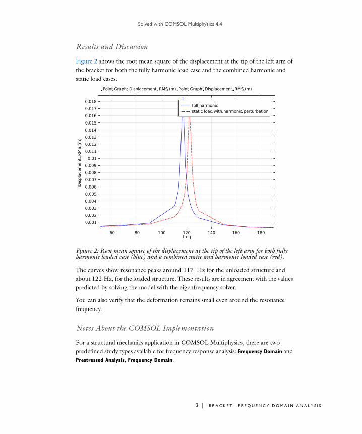
Solved with COMSOL Multiphysics 4.4
Results and Discussion
Figure 2 shows the root mean square of the displacement at the tip of the left arm of the bracket for both the fully harmonic load case and the combined harmonic and static load cases.
Figure 2: Root mean square of the displacement at the tip of the left arm for both fully harmonic loaded case (blue) and a combined static and harmonic loaded case (red).
The curves show resonance peaks around 117 Hz for the unloaded structure and about 122 Hz, for the loaded structure. These results are in agreement with the values predicted by solving the model with the eigenfrequency solver.
You can also verify that the deformation remains small even around the resonance frequency.
Notes About the COMSOL Implementation
For a structural mechanics application in COMSOL Multiphysics, there are two predefined study types available for frequency response analysis: Frequency Domain and Prestressed Analysis, Frequency Domain.
3 | B R A C K E T — F R E Q U E N C Y D O M A I N A N A L Y S I S

Solved with COMSOL Multiphysics 4.4
4 | B R A
The frequency domain analysis computes for the structural response of an harmonic load. All loads and boundary conditions are assumed to be harmonic.
Use the prestressed frequency response analysis when a structure is subjected to both static and harmonic loads, and the stiffness induced by the static load case can affect the structural response to the harmonic load.
Model Library path: Structural_Mechanics_Module/Tutorial_Models/bracket_frequency
Modeling Instructions
1 On the Home toolbar, click Model Library.
2 Go to the Model Library window. In the Model Library tree, select Structural Mechanics
Module>Tutorial Models>bracket basic.
3 Click Open Model.
C O M P O N E N T 1
On the Home toolbar, click Add Physics.
A D D P H Y S I C S
1 Go to the Add Physics window.
2 In the Add physics tree, select Structural Mechanics>Solid Mechanics.
3 In the Add physics window, click Add to Component.
R O O T
On the Home toolbar, click Add Study.
A D D S T U D Y
1 Go to the Add Study window.
2 Find the Studies subsection. In the tree, select Preset Studies>Frequency Domain.
3 In the Add study window, click Add Study.
C K E T — F R E Q U E N C Y D O M A I N A N A L Y S I S

Solved with COMSOL Multiphysics 4.4
S O L I D M E C H A N I C S
Damping 11 In the Model Builder window, under Component 1>Solid Mechanics right-click Linear
Elastic Material 1 and choose Damping.
In the frequency domain you can use loss factor damping or Rayleigh damping. For this example use loss factor damping.
2 In the Damping settings window, locate the Damping Settings section.
3 From the Damping type list, choose Isotropic loss factor.
M A T E R I A L S
Structural steelThe bracket is made of structural steel, which commonly has a damping ratio of a few percent. For this example, assume that the loss factor is 0.02.
1 In the Model Builder window, under Component 1>Materials click Structural steel.
2 In the Material settings window, locate the Material Contents section.
3 In the table, enter the following settings:
Set a displacement constraint for the mounting bolt domains.
S O L I D M E C H A N I C S
Fixed Constraint 11 On the Physics toolbar, click Domains and choose Fixed Constraint.
2 In the Fixed Constraint settings window, locate the Domain Selection section.
3 From the Selection list, choose Box 1.
You can now apply an external harmonic load to the bracket arms.
Boundary Load 11 On the Physics toolbar, click Boundaries and choose Boundary Load.
2 In the Boundary Load settings window, locate the Boundary Selection section.
3 From the Selection list, choose Box 2.
Property Name Value Unit Property group
Isotropic structural loss factor eta_s 0.02 1 Basic
5 | B R A C K E T — F R E Q U E N C Y D O M A I N A N A L Y S I S

Solved with COMSOL Multiphysics 4.4
6 | B R A
4 Locate the Force section. Specify the FA vector as
S T U D Y 1
Step 1: Frequency DomainThe frequency range will be 70 Hz-170 Hz with a refined frequency sweep step between 110 Hz and 130 Hz.
1 In the Model Builder window, expand the Study 1 node, then click Step 1: Frequency
Domain.
2 In the Frequency Domain settings window, locate the Study Settings section.
3 In the Frequencies edit field, type 50 70 90 110 range(111,1,130) 150 170 190.
4 On the Home toolbar, click Compute.
R E S U L T S
Stress (solid)The default plot group shows the stress distribution on a deformed geometry for the final frequency. You can change the frequency for the plot evaluation in the Parameter
value list of the plot group's Settings window.
Plot the root mean square of the displacement at the tip of the left arm of the bracket.
1D Plot Group 21 On the Home toolbar, click Add Plot Group and choose 1D Plot Group.
2 On the 1D plot group 2 toolbar, click Point Graph.
3 In the Point Graph settings window, locate the Selection section.
4 Click Paste Selection.
5 Go to the Paste Selection dialog box.
6 In the Selection edit field, type 1.
7 Click the OK button.
8 In the Point Graph settings window, click Replace Expression in the upper-right corner of the y-axis data section. From the menu, choose Solid
Mechanics>Displacement>Displacement, RMS (solid.disp_rms).
1e5 x
0 y
1e5 z
C K E T — F R E Q U E N C Y D O M A I N A N A L Y S I S

Solved with COMSOL Multiphysics 4.4
9 Click to expand the Legends section. Select the Show legends check box.
10 From the Legends list, choose Manual.
11 In the table, enter the following settings:
12 On the 1D Plot Group 2 toolbar, click Plot.
You will now consider a static load applied to the bracket and compute the prestressed frequency domain analysis.
A D D S T U D Y
1 Go to the Add Study window.
2 Find the Studies subsection. In the tree, select Preset Studies>Prestressed Analysis,
Frequency Domain.
3 In the Add study window, click Add Study.
S O L I D M E C H A N I C S
Boundary Load 21 On the Physics toolbar, click Boundaries and choose Boundary Load.
2 In the Boundary Load settings window, locate the Boundary Selection section.
3 From the Selection list, choose Box 2.
4 Locate the Coordinate System Selection section. From the Coordinate system list, choose Rotated System 2.
5 Locate the Force section. Specify the FA vector as
Boundary Load 1In the prestressed frequency response analysis, the load is assumed to be static by default. To define a harmonic load you need to mark the load feature node as being a harmonic perturbation.
1 In the Model Builder window, under Component 1>Solid Mechanics right-click Boundary Load 1 and choose Harmonic Perturbation.
Legends
full harmonic
0 x1
loadIntensity x2
0 x3
7 | B R A C K E T — F R E Q U E N C Y D O M A I N A N A L Y S I S

Solved with COMSOL Multiphysics 4.4
8 | B R A
S T U D Y 2
Step 2: Frequency-Domain, Perturbation1 In the Model Builder window, under Study 2 click Step 2: Frequency-Domain,
Perturbation.
2 In the Frequency-Domain, Perturbation settings window, locate the Study Settings section.
3 In the Frequencies edit field, type 50 70 90 110 range(111,1,130) 150 170 190.
4 On the Home toolbar, click Compute.
R E S U L T S
Stress (solid) 1You have previously created a point graph plot for the unloaded case. Add a new point graph plot to the same figure but use the data set of the second load case.
1D Plot Group 21 In the Model Builder window, under Results>1D Plot Group 2 right-click Point Graph
1 and choose Duplicate.
2 In the Point Graph settings window, locate the Data section.
3 From the Data set list, choose Solution 2.
4 Locate the y-Axis Data section. Clear the Compute differential check box.
5 Click to expand the Coloring and style section.
6 Find the Line style subsection. From the Line list, choose Dashed.
7 From the Color list, choose Red.
8 Locate the Legends section. In the table, enter the following settings:
9 On the 1D Plot Group 2 toolbar, click Plot.
Legends
static load with harmonic perturbation
C K E T — F R E Q U E N C Y D O M A I N A N A L Y S I S

Solved with COMSOL Multiphysics 4.4
B r a c k e t—In i t i a l - S t r a i n
Introduction
This tutorial model summarizes the fundamentals to model structural mechanics problems and how to apply them in COMSOL Multiphysics and the Structural Mechanics Module. In this example you will see how to defined prestrained structure and investigate how it affects the assembly.
It is recommended you review the Introduction to the Structural Mechanics Module, which includes background information and discusses the bracket_basic.mph model relevant to this example.
Model Definition
The model used in this guide is an assembly of a bracket and its mounting bolts, which are all made of steel. This type of bracket can be used to install an actuator that is mounted on a pin placed between the two holes in the bracket arms. The geometry is shown in Figure 1.
Figure 1: Bracket geometry.
1 | B R A C K E T — I N I T I A L - S T R A I N

Solved with COMSOL Multiphysics 4.4
2 | B R A
An initial strain simulates that the pin is prestrained in the axial direction, and investigate how it affects the assembly.
Results
Figure 2 shows how the pin compresses the bracket arms, and that the largest stresses are found in the region where the bracket arms are joined to the bolt supports.
Figure 2: Von Mises stress distribution in the bracket.
Figure 3 shows the x-component of the strain tensor to visualize the total strain in the structure. As the pin is stiff in comparison to the bracket, the total strain in the pin is almost the same as the initial strain given in the example.
C K E T — I N I T I A L - S T R A I N

Solved with COMSOL Multiphysics 4.4
Figure 3: Strain distribution in the bracket.
Notes About the COMSOL Implementation
Initial stresses and strains can be specified as a subfeature to a material model. You can define a stress/strain distribution with constant values or as an expression which can, for example, be space- or time-dependent. The initial stresses and strains can also be results from another study, or even from another physics interface in the same study.
Model Library path: Structural_Mechanics_Module/Tutorial_Models/bracket_initial_strain
Modeling Instructions
1 On the Home toolbar, click Model Libraries.
2 Go to the Model Libraries window. In the Model Libraries tree, select Structural
Mechanics Module>Tutorial Models>bracket basic.
3 Click Open Model.
3 | B R A C K E T — I N I T I A L - S T R A I N

Solved with COMSOL Multiphysics 4.4
4 | B R A
C O M P O N E N T 1
1 On the Home toolbar, click Add Physics.
A D D P H Y S I C S
1 Go to the Add Physics window.
2 In the Add Physics tree, select Structural Mechanics>Solid Mechanics (solid).
3 In the Add Physics window, click Add to Component.
4 On the Home toolbar, click Add Physics to close the Add Physics window.
R O O T
On the Home toolbar, click Add Study.
A D D S T U D Y
1 Go to the Add Study window.
2 Find the Studies subsection. In the tree, select Preset Studies>Stationary.
3 In the Add Study window, click Add Study.
4 On the Home toolbar, click Add Study to close the Add Study window.
G L O B A L D E F I N I T I O N S
ParametersIn the Parameters table, define a strain value that corresponds to a reduction of the pin length from 216 mm to 215 mm.
1 In the Model Builder window, under Global Definitions click Parameters.
2 In the Parameters settings window, locate the Parameters section.
3 In the table, enter the following settings:
G E O M E T R Y 1
The pin geometry is added to the bracket assembly. This is done by importing it into the existing geometry.
Name Expression Value Description
L0 216[mm] 0.2160 m Initial pin length
L 215[mm] 0.2150 m Current pin length
InitStrain (L-L0)/L0 -0.00463 Pin strain
C K E T — I N I T I A L - S T R A I N

Solved with COMSOL Multiphysics 4.4
Import 2 (imp2)1 On the Home toolbar, click Import.
2 In the Import settings window, locate the Import section.
3 From the Geometry import list, choose COMSOL Multiphysics file.
4 Click the Browse button.
5 Browse to the model’s Model Library folder and double-click the file bracket_pin.mphbin.
6 Click the Import button.
S O L I D M E C H A N I C S
Linear Elastic Material 1The initial strain is specified under the Linear Elastic Material node.
1 In the Model Builder window, expand the Component 1 >Solid Mechanics (solid) node.
Initial Stress and Strain 11 Right-click Linear Elastic Material 1 and choose Initial Stress and Strain.
2 In the Initial Stress and Strain settings window, locate the Domain Selection section.
3 From the Selection list, choose Manual.
4 Select Domain 3 only.
The prestrain direction is the axial direction of the bolt, which coincides with the global x direction.
5 Locate the Initial Stress and Strain section. In the 0 table, enter the following settings:
Fixed Constraint 11 On the Physics toolbar, click Domains and choose Fixed Constraint.
2 In the Fixed Constraint settings window, locate the Domain Selection section.
3 From the Selection list, choose Box 1.
S T U D Y 1
On the Home toolbar, click Compute.
InitStrain 0 0
0 0 0
0 0 0
5 | B R A C K E T — I N I T I A L - S T R A I N

Solved with COMSOL Multiphysics 4.4
6 | B R A
R E S U L T S
3D Plot Group 21 On the Home toolbar, click Add Plot Group and choose 3D Plot Group.
2 In the Model Builder window, under Results right-click 3D Plot Group 2 and choose Surface.
3 In the Surface settings window, locate the Expression section.
4 Click Replace Expression in the upper-right corner and choose Solid
Mechanics>Strain>Strain tensor (material)>Strain tensor, XX component (solid.eXX). Double-click or press Enter.
5 On the 3D Plot Group 2 toolbar, click Plot.
6 Click the Go to Default 3D View button on the Graphics toolbar.
C K E T — I N I T I A L - S T R A I N

Solved with COMSOL Multiphysics 4.4
B r a c k e t—L in e a r Bu c k l i n g
Introduction
Linear buckling analysis is an important study type in structural analysis because it provides an estimate of the critical load that can cause sudden collapse of the structure. In this example you will see how to perform a linear buckling analysis.
It is recommended you review the Introduction to the Structural Mechanics Module, which includes background information and discusses the bracket_basic.mph model relevant to this example.
Model Definition
This model is an extension to the model example described in the section “The Fundamentals: A Static Linear Analysis” in the Introduction to the Structural Mechanics Module.
Due to the symmetry, the model uses only one half of the entire geometry. The model geometry is represented in Figure 1.
Figure 1: Bracket geometry.
1 | B R A C K E T — L I N E A R B U C K L I N G

Solved with COMSOL Multiphysics 4.4
2 | B R A
The current analysis computes the critical compressive load oriented in the positive y-direction.
Results and Discussion
Figure 2 shows the first buckling mode for the bracket geometry. The critical load factor is about 1.5e8 which correspond to a critical buckling load that is slightly lower than 6000 N.
Figure 2: First buckling mode and critical load factor value.
Notes About the COMSOL Implementation
A linear buckling analysis consists of the following operations:
• Perform a static analysis using a unit load.
• Compute the eigenvalue problem including the stresses from the static load. The first eigenvalue corresponds to the value of the critical buckling load.
COMSOL runs automatically the sequence described above and the returns the value of the critical buckling load.
C K E T — L I N E A R B U C K L I N G

Solved with COMSOL Multiphysics 4.4
Model Library path: Structural_Mechanics_Module/Tutorial_Models/bracket_linear_buckling
Modeling Instructions
1 On the Home toolbar, click Model Library.
2 Go to the Model Library window. In the Model Library tree, select Structural Mechanics
Module>Tutorial Models>bracket basic.
3 Click Open Model.
C O M P O N E N T 1
1 On the Home toolbar, click Add Physics.
A D D P H Y S I C S
1 Go to the Add Physics window.
2 In the Add physics tree, select Structural Mechanics>Solid Mechanics.
3 In the Add physics window, click Add to Component.
R O O T
On the Home toolbar, click Add Study.
A D D S T U D Y
1 Go to the Add Study window.
2 Find the Studies subsection. In the tree, select Preset Studies>Linear Buckling.
3 In the Add study window, click Add Study.
G E O M E T R Y 1
Import 1 (imp1)1 In the Model Builder window, under Component 1 >Geometry 1 click Import 1 (imp1).
2 In the Import settings window, locate the Import section.
3 Click the Browse button.
4 Browse to the model’s Model Library folder and double-click the file bracket_symmetry.mphbin.
5 Click the Import button.
3 | B R A C K E T — L I N E A R B U C K L I N G

Solved with COMSOL Multiphysics 4.4
4 | B R A
6 Click the Go to Default 3D View button on the Graphics toolbar.
7 Click the Zoom Extents button on the Graphics toolbar.
G L O B A L D E F I N I T I O N S
ParametersFor this example, you need to change the orientation and the magnitude of the load applied to the bracket. Use a unit load and set the angle that defines the orientation of the load to 0.
1 In the Model Builder window, expand the Global Definitions node, then click Parameters.
2 In the Parameters settings window, locate the Parameters section.
3 In the table, enter the following settings:
S O L I D M E C H A N I C S
Add displacement constraints and a boundary load so that the mounting bolts are fully constrained and the unit load is applied to the bracket hole. Finally apply a symmetry condition at the boundary in the symmetry plane.
Fixed Constraint 11 On the Physics toolbar, click Domains and choose Fixed Constraint.
2 In the Fixed Constraint settings window, locate the Domain Selection section.
3 From the Selection list, choose Box 1.
Symmetry 11 On the Physics toolbar, click Boundaries and choose Symmetry.
2 Select Boundaries 43 and 44 only.
Boundary Load 11 On the Physics toolbar, click Boundaries and choose Boundary Load.
2 In the Boundary Load settings window, locate the Boundary Selection section.
3 From the Selection list, choose Box 2.
4 Locate the Coordinate System Selection section. From the Coordinate system list, choose Rotated System 2 (sys2).
Name Expression Value Description
theta0 0[deg] 0 rad Direction of load
P0 1[Pa] 1.000 Pa Peak load intensity
C K E T — L I N E A R B U C K L I N G

Solved with COMSOL Multiphysics 4.4
5 Locate the Force section. Specify the FA vector as
S T U D Y 1
On the Home toolbar, click Compute.
R E S U L T S
Mode Shape (solid)The default plot shows the mode shape of the first buckling mode.
Derived ValuesTo obtain the critical buckling load you need to multiply the applied load by the eigenvalue (Critical load factor) returned by the linear buckling analysis.
1 On the Results toolbar, click More Derived Values and choose Integration>Surface
Integration.
2 In the Surface Integration settings window, locate the Selection section.
3 From the Selection list, choose Box 2.
4 Locate the Expression section. In the Expression edit field, type lambda*loadIntensity.
5 Click the Evaluate button.
0 x1
loadIntensity x2
0 x3
5 | B R A C K E T — L I N E A R B U C K L I N G

Solved with COMSOL Multiphysics 4.4
6 | B R A
C K E T — L I N E A R B U C K L I N G
Solved with COMSOL Multiphysics 4.4
B r a c k e t—Parame t r i c Ana l y s i s
Introduction
This tutorial model summarizes the fundamentals to model structural mechanics problems and how to apply them in COMSOL Multiphysics and the Structural Mechanics Module. This includes computing the solution for several parameter values in a continuation.
It is recommended you review the Introduction to the Structural Mechanics Module, which includes background information and discusses the bracket_basic.mph model relevant to this example.
Model Definition
This model is an extension to the model example described in the section “The Fundamentals: A Static Linear Analysis” in the Introduction to the Structural Mechanics Module.
The geometry is shown in Figure 1.
Figure 1: Bracket geometry.
1 | B R A C K E T — P A R A M E T R I C A N A L Y S I S
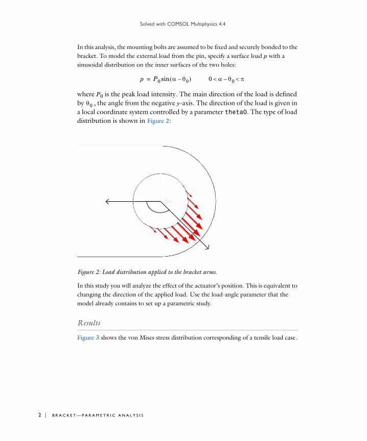
Solved with COMSOL Multiphysics 4.4
2 | B R A
In this analysis, the mounting bolts are assumed to be fixed and securely bonded to the bracket. To model the external load from the pin, specify a surface load p with a sinusoidal distribution on the inner surfaces of the two holes:
where P0 is the peak load intensity. The main direction of the load is defined by , the angle from the negative y-axis. The direction of the load is given in a local coordinate system controlled by a parameter theta0. The type of load distribution is shown in Figure 2:
Figure 2: Load distribution applied to the bracket arms.
In this study you will analyze the effect of the actuator’s position. This is equivalent to changing the direction of the applied load. Use the load-angle parameter that the model already contains to set up a parametric study.
Results
Figure 3 shows the von Mises stress distribution corresponding of a tensile load case.
p P0 0– 0 0– sin=
0
C K E T — P A R A M E T R I C A N A L Y S I S
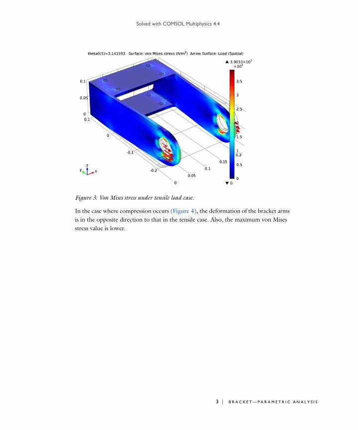
Solved with COMSOL Multiphysics 4.4
Figure 3: Von Mises stress under tensile load case.
In the case where compression occurs (Figure 4), the deformation of the bracket arms is in the opposite direction to that in the tensile case. Also, the maximum von Mises stress value is lower.
3 | B R A C K E T — P A R A M E T R I C A N A L Y S I S

Solved with COMSOL Multiphysics 4.4
4 | B R A
Figure 4: Von Mises stress under compressive load case.
Figure 5 shows the stress distribution for a bending load case. The maximum stress values are no longer located around the holes but in the region where the arms connect to the bolt supports.
C K E T — P A R A M E T R I C A N A L Y S I S

Solved with COMSOL Multiphysics 4.4
Figure 5: Von Mises stress under bending load case.
Figure 6 shows that the reaction force in the y direction is symmetric around 90o—negative from 0o to 90o and positive from 90o to 180o. The reaction force in the z direction has a maximum at 90o.
5 | B R A C K E T — P A R A M E T R I C A N A L Y S I S
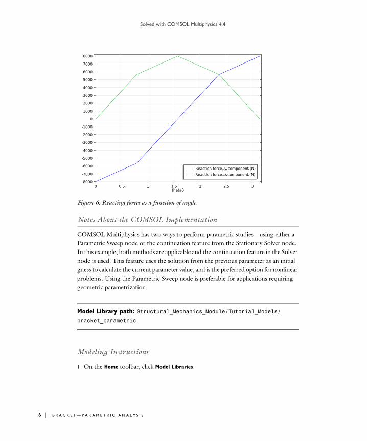
Solved with COMSOL Multiphysics 4.4
6 | B R A
Figure 6: Reacting forces as a function of angle.
Notes About the COMSOL Implementation
COMSOL Multiphysics has two ways to perform parametric studies—using either a Parametric Sweep node or the continuation feature from the Stationary Solver node. In this example, both methods are applicable and the continuation feature in the Solver node is used. This feature uses the solution from the previous parameter as an initial guess to calculate the current parameter value, and is the preferred option for nonlinear problems. Using the Parametric Sweep node is preferable for applications requiring geometric parametrization.
Model Library path: Structural_Mechanics_Module/Tutorial_Models/bracket_parametric
Modeling Instructions
1 On the Home toolbar, click Model Libraries.
C K E T — P A R A M E T R I C A N A L Y S I S

Solved with COMSOL Multiphysics 4.4
2 Go to the Model Libraries window. In the Model Libraries tree, select Structural
Mechanics Module>Tutorial Models>bracket static.
3 Click Open Model.
C O M P O N E N T 1
Parametric studies can be set up from scratch or, as in this example, added to an existing study.
S T U D Y 1
Step 1: Stationary1 In the Model Builder window, expand the Study 1 node, then click Step 1: Stationary.
2 In the Stationary settings window, click to expand the Study Extensions section.
3 Locate the Study Extensions section. Select the Auxiliary sweep check box.
4 From the Run continuation for list, choose No parameter.
5 Click Add.
6 In the table, enter the following settings:
7 Click Range.
8 Go to the Range dialog box.
9 In the Start edit field, type 0.
10 In the Stop edit field, type 180[deg].
11 In the Step edit field, type 45[deg].
12 Click the Add button.
13 On the Home toolbar, click Compute.
R E S U L T S
Stress (solid)1 In the 3D Plot Group settings window, locate the Data section.
2 From the Parameter value (theta0) list, choose 0.
3 On the Stress (solid) toolbar, click Plot.
4 From the Parameter value (theta0) list, choose 1.570796.
Auxiliary parameter Parameter value list
theta0
7 | B R A C K E T — P A R A M E T R I C A N A L Y S I S

Solved with COMSOL Multiphysics 4.4
8 | B R A
5 On the Stress (solid) toolbar, click Plot.
Derived Values1 On the Results toolbar, click More Derived Values and choose Integration>Volume
Integration.
2 In the Volume Integration settings window, locate the Selection section.
3 From the Selection list, choose Box 1.
4 Click the Replace Expression in the upper-right corner of the Expression section. From the menu, choose Solid Mechanics>Reactions>Reaction force (Spatial)>Reaction
force, y component (solid.RFy). Double-click or press Enter.
5 Click the Evaluate button.
6 In the Volume Integration settings window, locate the Expression section.
7 Click the Replace Expression in the upper-right corner of the Expression section. From the menu, choose Solid Mechanics>Reactions>Reaction force (Spatial)>Reaction
force, z component (solid.RFz). Double-click or press Enter.
8 Click the Evaluate button.
9 In the Table window, click Table Graph.
1D Plot Group 41 In the Model Builder window, under Results click 1D Plot Group 4.
2 In the 1D Plot Group settings window, click to expand the Legend section.
3 From the Position list, choose Lower right.
4 In the Model Builder window, under Results>1D Plot Group 4 click Table Graph 1.
5 In the Table Graph settings window, click to expand the Legends section.
6 Select the Show legends check box.
===================
From the File menu, choose Open.
Browse to the model’s Model Library folder and double-click the file bracket_static.mph.
R E S U L T S
C O M P O N E N T 1
Parametric studies can be set up from scratch or, as in this example, added to an existing study.
C K E T — P A R A M E T R I C A N A L Y S I S

Solved with COMSOL Multiphysics 4.4
S T U D Y 1
Step 1: Stationary1 In the Model Builder window, expand the Study 1 node, then click Step 1: Stationary.
2 In the Stationary settings window, click to expand the Study extensions section.
3 Locate the Study Extensions section. Select the Auxiliary sweep check box.
4 From the Run continuation for list, choose No parameter.
5 Click Add.
6 In the table, enter the following settings:
7 Click Range.
8 Go to the Range dialog box.
9 In the Start edit field, type 0.
10 In the Stop edit field, type 180[deg].
11 In the Step edit field, type 45[deg].
12 Click the Add button.
13 On the Home toolbar, click Compute.
R E S U L T S
Stress (solid)1 Click the Zoom Extents button on the Graphics toolbar.
2 In the 3D Plot Group settings window, locate the Data section.
3 From the Parameter value (theta0) list, choose 0.
4 On the 3D plot group toolbar, click Plot.
5 From the Parameter value (theta0) list, choose 1.570796.
6 On the 3D plot group toolbar, click Plot.
Derived Values1 On the Results toolbar, click More Derived Values and choose Integration>Volume
Integration.
2 In the Volume Integration settings window, locate the Selection section.
3 From the Selection list, choose Box 1.
Auxiliary parameter Parameter value list
theta0
9 | B R A C K E T — P A R A M E T R I C A N A L Y S I S

Solved with COMSOL Multiphysics 4.4
10 | B R
4 Click Replace Expression in the upper-right corner of the Expression section. From the menu, choose Solid Mechanics>Reactions>Reaction force (Spatial)>Reaction force,
y component (solid.RFy).
5 Click the Evaluate button.
6 In the Volume Integration settings window, click Replace Expression in the upper-right corner of the Expression section. From the menu, choose Solid
Mechanics>Reactions>Reaction force (Spatial)>Reaction force, z component (solid.RFz).
7 In the Table window, click Table Graph.
1D Plot Group 41 In the Model Builder window, under Results click 1D Plot Group 4.
2 In the 1D Plot Group settings window, click to expand the Legend section.
3 From the Position list, choose Lower right.
4 In the Model Builder window, under Results>1D Plot Group 4 click Table Graph 1.
5 In the Table Graph settings window, click to expand the Legends section.
6 Select the Show legends check box.
A C K E T — P A R A M E T R I C A N A L Y S I S

Solved with COMSOL Multiphysics 4.4
B r a c k e t—Rig i d Conn e c t o r
Introduction
Using rigid connectors provides an alternative to having to model a geometric entity that is not significantly affected by a structural analysis. It allows the replacement of parts of an elastic structure with rigid bodies, where a for example a boundary condition is defined. This saves computational time and memory.
In this example, you will study the stress in a bracket connected to a pin where a load is applied. The pin is simulated as a rigid connector
It is recommended you review the Introduction to the Structural Mechanics Module, which includes background information and discusses the bracket_basic.mph model relevant to this example.
Model Definition
This model is an extension to the model example described in the section “The Fundamentals: A Static Linear Analysis” in the Introduction to the Structural Mechanics Module.
The model geometry is represented in Figure 1.
Figure 1: Bracket geometry.
1 | B R A C K E T — R I G I D C O N N E C T O R

Solved with COMSOL Multiphysics 4.4
2 | B R A
A pin is connected between the bracket hole where a load is applied. The pin is assumed to be perfectly rigid and modeled with a rigid connector. Thus the pin is not represented in the model geometry. Figure 2 below shows the boundaries connected to the rigid connector and the position of its center of rotation.
Figure 2: Center of rotation of the rigid connector applied to the bracket geometry.
Results and Discussion
Figure 3 shows the von Mises stress on a deformed geometry. You can see the effect that the pin’s rotation and applied force has on the bracket arms.
C K E T — R I G I D C O N N E C T O R

Solved with COMSOL Multiphysics 4.4
Figure 3: Von Mises stress distribution.
Notes About the COMSOL Implementation
The rigid connector has the translational and rotational degrees of freedom of a rigid body. Options for this feature include applying an external load or moment to the rigid body, or defining mass and moments of inertia in dynamic analyses. The rigid connector feature can also be used to apply loads and constraints at points so that these are distributed and thereby preventing singularities.
Model Library path: Structural_Mechanics_Module/Tutorial_Models/bracket_rigid_connector
Modeling Instructions
1 On the Home toolbar, click Model Libraries.
3 | B R A C K E T — R I G I D C O N N E C T O R

Solved with COMSOL Multiphysics 4.4
4 | B R A
2 Go to the Model Libraries window. In the Model Libraries tree, select Structural
Mechanics Module>Tutorial Models>bracket basic.
3 Click Open Model.
C O M P O N E N T 1
1 On the Home toolbar, click Add Physics.
A D D P H Y S I C S
1 Go to the Add Physics window.
2 In the Add physics tree, select Structural Mechanics>Solid Mechanics (solid).
3 In the Add physics window, click Add to Component.
4 On the Home toolbar, click Add Physics to close the Add Physics window.
R O O T
On the Home toolbar, click Add Study.
A D D S T U D Y
1 Go to the Add Study window.
2 Find the Studies subsection. In the tree, select Preset Studies>Stationary.
3 In the Add study window, click Add Study.
4 On the Home toolbar, click Add Study to close the Add Study window.
S O L I D M E C H A N I C S
Rigid Connector 11 On the Physics toolbar, click Boundaries and choose Rigid Connector.
Now add a rigid connector that connects the holes in the bracket arms to simulate the presence of the pin.
2 In the Rigid Connector settings window, locate the Boundary Selection section.
3 From the Selection list, choose Box 2.
By default the location of the center of rotation is computed automatically. To visualize its position you need to enable the physics symbols. This is done in the File
C K E T — R I G I D C O N N E C T O R

Solved with COMSOL Multiphysics 4.4
menu, where you select Preferences. In the Preferences window, click Graphics. In the Visualization section select Show physics symbols.
If you wish to specify the location of the center of rotation yourself, select User
defined in the Center of rotation list.
Below, you use the rigid connector feature to analyze the stress distribution in the bracket under the assumption that the pin rotates 1 degree around the y-axis. The center of rotation is defined as the midpoint between the arms.
The displacements of the rigid connector are constrained in the x and z directions.
4 Locate the Prescribed Displacement at Center of Rotation section. Select the Prescribed in x direction check box.
5 Select the Prescribed in z direction check box.
6 Locate the Prescribed Rotation at Center of Rotation section. From the By list, choose Prescribed rotation at center of rotation.
Apply a prescribed rotation of the rigid body of 1 degree around the y-axis.
7 Specify the vector as
8 In the 0 edit field, type 1[deg].
Applied Force 11 Right-click Component 1 >Solid Mechanics >Rigid Connector 1 and choose Applied
Force.
Apply an external load of 100 N at the center of rotation of the rigid body.
2 In the Applied Force settings window, locate the Applied Force section.
3 Specify the F vector as
Fixed Constraint 11 On the Physics toolbar, click Domains and choose Fixed Constraint.
2 In the Fixed Constraint settings window, locate the Domain Selection section.
0 x
1 y
0 z
0 x
-100[N] y
0 z
5 | B R A C K E T — R I G I D C O N N E C T O R

Solved with COMSOL Multiphysics 4.4
6 | B R A
3 From the Selection list, choose Box 1.
S T U D Y 1
On the Home toolbar, click Compute.
R E S U L T S
Stress (solid)1 Click the Zoom Extents button on the Graphics toolbar.
The default plot shows the von Mises stress on a deformed geometry.
C K E T — R I G I D C O N N E C T O R

Solved with COMSOL Multiphysics 4.4
B r a c k e t—She l l
Introduction
For thin geometries it can be more efficient to use shell elements instead of solid elements, thus saving computational time and memory. The Shell interface in the Structural Mechanics Module can be used to model structures approximated by thin and thick shells. There is also a similar Plate interface for 2D problems. The thickness of the shell or plate is taken into account in the equations instead of being explicitly modeled in the geometry.
In this example you will study the stress in a bracket subjected to external loads. The bracket is modeled with the Shell interface.
It is recommended you review the Introduction to the Structural Mechanics Module, which includes background information and discusses the bracket_basic.mph model relevant to this example.
Model Definition
This model is an extension to the model example described in the section “The Fundamentals: A Static Linear Analysis” in the Introduction to the Structural Mechanics Module.
The shell geometry of the bracket comes from the midplane of the solid geometry. The model geometry is represented in Figure 1.
1 | B R A C K E T — S H E L L

Solved with COMSOL Multiphysics 4.4
2 | B R A
Figure 1: Bracket geometry.
The load is applied along the edge at the bracket holes.
Results and Discussion
Figure 2 shows the von Mises stress on a deformed geometry.
C K E T — S H E L L
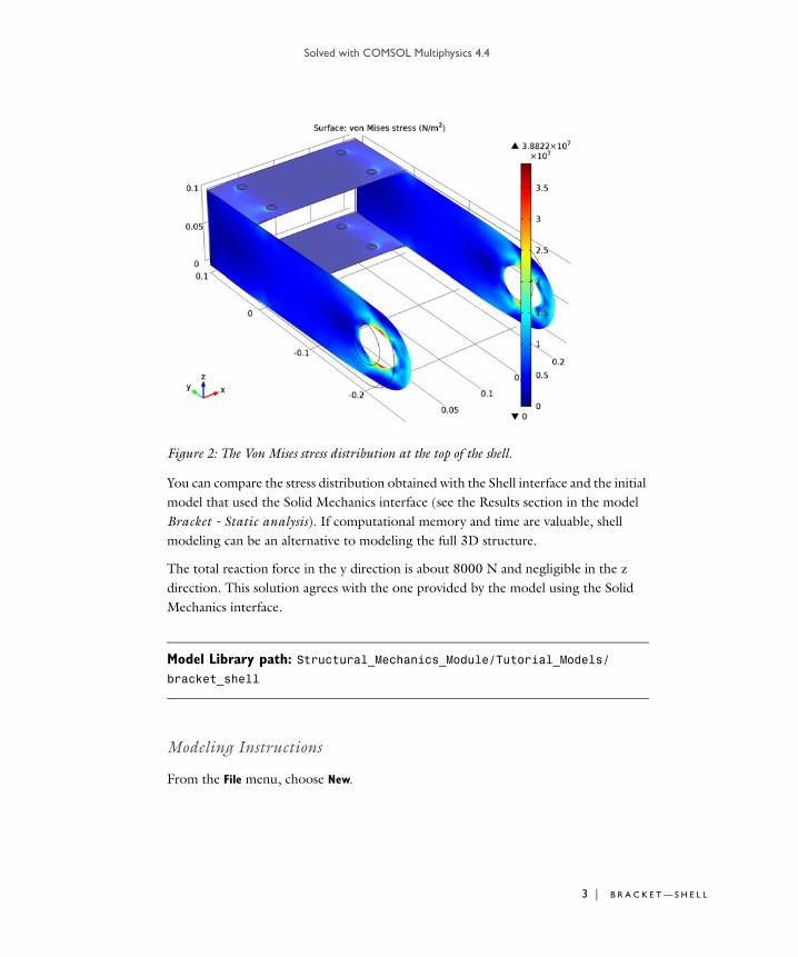
Solved with COMSOL Multiphysics 4.4
Figure 2: The Von Mises stress distribution at the top of the shell.
You can compare the stress distribution obtained with the Shell interface and the initial model that used the Solid Mechanics interface (see the Results section in the model Bracket - Static analysis). If computational memory and time are valuable, shell modeling can be an alternative to modeling the full 3D structure.
The total reaction force in the y direction is about 8000 N and negligible in the z direction. This solution agrees with the one provided by the model using the Solid Mechanics interface.
Model Library path: Structural_Mechanics_Module/Tutorial_Models/bracket_shell
Modeling Instructions
From the File menu, choose New.
3 | B R A C K E T — S H E L L

Solved with COMSOL Multiphysics 4.4
4 | B R A
N E W
1 In the New window, click the Model Wizard button.
M O D E L W I Z A R D
1 In the Model Wizard window, click the 3D button.
2 In the Select physics tree, select Structural Mechanics>Shell.
3 Click the Add button.
4 Click the Study button.
5 In the tree, select Preset Studies>Stationary.
6 Click the Done button.
G L O B A L D E F I N I T I O N S
Parameters1 On the Home toolbar, click Parameters.
2 In the Parameters settings window, locate the Parameters section.
3 In the table, enter the following settings:
G E O M E T R Y 1
Import 1 (imp1)1 On the Home toolbar, click Import.
2 In the Import settings window, locate the Import section.
3 From the Geometry import list, choose COMSOL Multiphysics file.
4 Click the Browse button.
5 Browse to the model’s Model Library folder and double-click the file bracket_shell.mphbin.
6 Click the Import button.
Name Expression Value Description
theta0 180[deg] 3.142 rad Direction of load
P0 1e7[Pa] 1.000E7 Pa Peak load intensity
y0 -200[mm] -0.2000 m Y center of hole
z0 50[mm] 0.05000 m Z center of hole
C K E T — S H E L L

Solved with COMSOL Multiphysics 4.4
D E F I N I T I O N S
Explicit 11 On the Definitions toolbar, click Explicit.
Define some explicit selections for easy access during the modeling procedure. The first selection consists of the boundaries representing the mounting bolts.
2 In the Explicit settings window, locate the Input Entities section.
3 From the Geometric entity level list, choose Boundary.
4 Select Boundaries 4–11 only.
Explicit 21 On the Definitions toolbar, click Explicit.
The second selection consists of the edges around the bracket holes.
2 In the Explicit settings window, locate the Input Entities section.
3 From the Geometric entity level list, choose Edge.
4 Select Edges 3, 4, 6, 7, 50, 51, 53, and 54 only.
Variables 11 In the Model Builder window, right-click Definitions and choose Variables.
The expression for the load intensity includes a logical operator ensuring that the load is only applied in the positive direction.
2 In the Variables settings window, locate the Variables section.
3 In the table, enter the following settings:
M A T E R I A L S
Now add structural steel material properties to the geometry.
1 On the Home toolbar, click Add Material.
A D D M A T E R I A L
1 Go to the Add Material window.
2 In the tree, select Built-In>Structural steel.
3 In the Add material window, click Add to Component.
Name Expression Unit Description
angle atan2((y-y0),(z-z0)) rad
loadIntensity P0*sin(angle-theta0)*(sin(angle-theta0)>0)
Pa
5 | B R A C K E T — S H E L L

Solved with COMSOL Multiphysics 4.4
6 | B R A
S H E L L
Using the Shell interface, the thickness of the structure is not represented in the geometry, so you must define it in the settings so that your model solves the physical problem.
1 In the Model Builder window, under Component 1 click Shell.
2 In the Shell settings window, locate the Thickness section.
3 In the d edit field, type 0.08.
You can add a Change Thickness node to the Shell interface to change the thickness of parts of the structure.
Fixed Constraint 11 On the Physics toolbar, click Boundaries and choose Fixed Constraint.
2 In the Fixed Constraint settings window, locate the Boundary Selection section.
3 From the Selection list, choose Explicit 1.
Edge Load 11 On the Physics toolbar, click Edges and choose Edge Load.
2 In the Edge Load settings window, locate the Edge Selection section.
3 From the Selection list, choose Explicit 2.
4 Locate the Force section. From the Load type list, choose Load defined as force per
unit area.
5 Specify the FA vector as
Since the load is fixed in the negative y-direction in this example, you do not need to use any local coordinate systems. If the parameter theta0 was selected to some other angle, then a more general input using a local coordinate system would have been needed.
S T U D Y 1
On the Home toolbar, click Compute.
0 x
-loadIntensity y
0 z
C K E T — S H E L L

Solved with COMSOL Multiphysics 4.4
R E S U L T S
Stress TopThe default plots show the von Mises stress at the two extreme locations in the shell thickness direction.
You can also manually define where in the thickness direction of the shell you want to plot the results. Do this by changing the location in the Surface Settings window under the Parameters definitions. There the parameter shell.z defines the height of evaluation in shell: 1 for the top surface, 0 for the mid plane, and -1 for the bottom surface.
Derived ValuesThe last step is to evaluate the reaction forces at the boundaries that represent the mounting bolts.
1 On the Results toolbar, click More Derived Values and choose Integration>Surface
Integration.
2 In the Surface Integration settings window, locate the Selection section.
3 From the Selection list, choose Explicit 1.
4 Locate the Expression section. Click Replace Expression in the upper-right corner of the Expression section. From the menu choose Shell>Reaction force, y component
(shell.RFy). Click the Evaluate button.
5 Click Replace Expression in the upper-right corner of the Expression section. From the menu choose Shell>Reaction force, z component (shell.RFz). Click the Evaluate button.
7 | B R A C K E T — S H E L L

Solved with COMSOL Multiphysics 4.4
8 | B R A
C K E T — S H E L L
Solved with COMSOL Multiphysics 4.4
B r a c k e t—Sp r i n g Founda t i o n Ana l y s i s
Introduction
A fixed, fully constrained, boundary condition contains the assumption that the analyzed structure is attached to an infinitely stiff support. While in many cases this is a good approximation, sometimes you may need to consider the stiffness of the supporting structure in your model. In COMSOL Multiphysics you can do this by using the Spring Foundation boundary condition.
In this example, you will study the stress in a bracket subjected to external loads. The stiffness of the mounted bolts connecting support is modeled with spring foundations.
It is recommended you review the Introduction to the Structural Mechanics Module, which includes background information and discusses the bracket_basic.mph model relevant to this example.
Model Definition
This model is an extension to the model example described in the section “The Fundamentals: A Static Linear Analysis” in the Introduction to the Structural Mechanics Module.
The model geometry is represented in Figure 1.
1 | B R A C K E T — S P R I N G F O U N D A T I O N A N A L Y S I S

Solved with COMSOL Multiphysics 4.4
2 | B R A
Figure 1: Bracket geometry.
The load is applied at the pin hole in the y-z plan with an orientation of 45 degrees from the negative y-axis.
The bolts are assumed to be elastic, defined with spring foundations.
Results and Discussion
Figure 2 shows the von Mises stress on a deformed geometry.
C K E T — S P R I N G F O U N D A T I O N A N A L Y S I S

Solved with COMSOL Multiphysics 4.4
Figure 2: The Von Mises stress distribution.
You can see the effect of using the spring condition instead of rigidly mounting the bolts (see the Results section in the model Bracket - Static analysis). The maximum stress is lower, while most of the deformation of the bracket occurs at its bolt’s support as opposed to in the vicinity of the holes.
Model Library path: Structural_Mechanics_Module/Tutorial_Models/bracket_spring
Modeling Instructions
1 On the Home toolbar, click Model Library.
2 Go to the Model Library window. In the Model Library tree, select Structural Mechanics
Module>Tutorial Models>bracket basic.
3 Click Open Model.
3 | B R A C K E T — S P R I N G F O U N D A T I O N A N A L Y S I S

Solved with COMSOL Multiphysics 4.4
4 | B R A
C O M P O N E N T 1
1 On the Home toolbar, click Add Physics.
A D D P H Y S I C S
1 Go to the Add Physics window.
2 In the Add physics tree, select Structural Mechanics>Solid Mechanics (solid).
3 In the Add physics window, click Add to Component.
R O O T
On the Home toolbar, click Add Study.
A D D S T U D Y
1 Go to the Add Study window.
2 Find the Studies subsection. In the tree, select Preset Studies>Stationary.
3 In the Add study window, click Add Study.
G L O B A L D E F I N I T I O N S
ParametersThe analysis is performed for the load angle, theta0 = 45 degrees, which is defined in the Parameters list. Two new parameters for the spring coefficients of the external structure are also defined.
1 In the Model Builder window, under Global Definitions click Parameters.
2 In the Parameters settings window, locate the Parameters section.
3 In the table, append the following parameter settings:
S O L I D M E C H A N I C S
As with all domain and boundary conditions, the Spring Foundation feature is found under the physics interface node, Solid Mechanics.
Spring Foundation 11 On the Physics toolbar, click Boundaries and choose Spring Foundation.
Name Expression Value Description
theta0 45[deg] 0.7854 rad Direction of load
kn 2e8[N/m] 2.000E8 N/m Normal spring coefficient
kt 1e8[N/m] 1.000E8 N/m Tangent spring coefficient
C K E T — S P R I N G F O U N D A T I O N A N A L Y S I S

Solved with COMSOL Multiphysics 4.4
2 Select Boundaries 22, 25, 30, 33, 46, 49, 54, and 57 only.
3 In the Spring Foundation settings window, locate the Spring section.
4 From the Spring type list, choose Total spring constant.
5 Specify the ktot vector as
Boundary Load 11 On the Physics toolbar, click Boundaries and choose Boundary Load.
2 In the Boundary Load settings window, locate the Boundary Selection section.
3 From the Selection list, choose Box 2.
4 Locate the Coordinate System Selection section. From the Coordinate system list, choose Rotated System 2 (sys2).
5 Locate the Force section. Specify the FA vector as
S T U D Y 1
On the Home toolbar, click Compute.
R E S U L T S
Stress (solid)1 Click the Zoom Extents button on the Graphics toolbar.
The default plot shows the von Mises effective stress distribution.
kt x
kt y
kn z
0 x1
loadIntensity x2
0 x3
5 | B R A C K E T — S P R I N G F O U N D A T I O N A N A L Y S I S

Solved with COMSOL Multiphysics 4.4
6 | B R A
C K E T — S P R I N G F O U N D A T I O N A N A L Y S I S
Solved with COMSOL Multiphysics 4.4
B r a c k e t—Sta t i c Ana l y s i s
Introduction
This tutorial model summarizes the fundamentals to model structural mechanics problems and how to apply them in COMSOL Multiphysics and the Structural Mechanics Module. This includes creating a geometry as well as defining material properties and boundary constraints and conditions. After the solution is computed, you will learn how to analyze results and check the reaction forces.
Model Definition
The model used in this guide is an assembly of a bracket and its mounting bolts, which are all made of steel. This type of bracket can be used to install an actuator that is mounted on a pin placed between the two holes in the bracket arms. The geometry is shown in Figure 1.
Figure 1: Bracket geometry.
1 | B R A C K E T — S T A T I C A N A L Y S I S

Solved with COMSOL Multiphysics 4.4
2 | B R A
In this analysis, the mounting bolts are assumed to be fixed and securely bonded to the bracket. To model the external load from the pin, specify a surface load p with a sinusoidal distribution on the inner surfaces of the two holes:
where P0 is the peak load intensity. The main direction of the load is defined by , the angle from the negative y-axis. The direction of the load is given in a local coordinate system controlled by a parameter theta0. The type of load distribution is shown in Figure 2:
Figure 2: Load distribution applied to the bracket arms..
In this study, the load will be pointing along the negative y-axis only.
Results
Figure 3 shows the von Mises stress distribution together with an exaggerated (automatically scaled) picture of the deformation. As expected, the high stress values are located around the holes and in the vicinity of the mounting bolts. The maximum von Mises stress remains below the yield stress value for structural steel which validates the choice of a linear elastic material to analyze this structure.
p P0 0– 0 0– sin=
0
C K E T — S T A T I C A N A L Y S I S

Solved with COMSOL Multiphysics 4.4
Figure 3: Von Mises stress distribution in the bracket under tensile load in y-axis direction.
In Figure 4 you can see that the bracket base remains fixed while only the arms are deformed. The maximum total displacement is about 27 m, which is in agreement with the assumption of small deformations.
3 | B R A C K E T — S T A T I C A N A L Y S I S
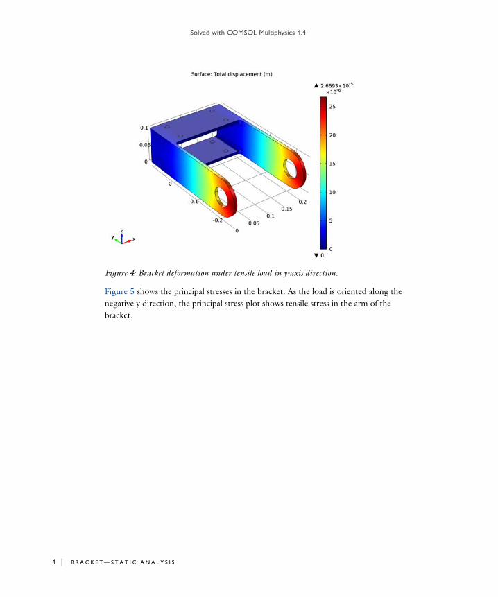
Solved with COMSOL Multiphysics 4.4
4 | B R A
Figure 4: Bracket deformation under tensile load in y-axis direction.
Figure 5 shows the principal stresses in the bracket. As the load is oriented along the negative y direction, the principal stress plot shows tensile stress in the arm of the bracket.
C K E T — S T A T I C A N A L Y S I S
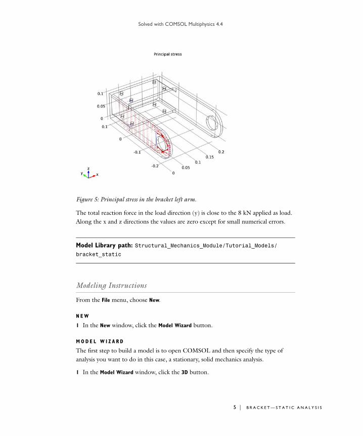
Solved with COMSOL Multiphysics 4.4
Figure 5: Principal stress in the bracket left arm.
The total reaction force in the load direction (y) is close to the 8 kN applied as load. Along the x and z directions the values are zero except for small numerical errors.
Model Library path: Structural_Mechanics_Module/Tutorial_Models/bracket_static
Modeling Instructions
From the File menu, choose New.
N E W
1 In the New window, click the Model Wizard button.
M O D E L W I Z A R D
The first step to build a model is to open COMSOL and then specify the type of analysis you want to do in this case, a stationary, solid mechanics analysis.
1 In the Model Wizard window, click the 3D button.
5 | B R A C K E T — S T A T I C A N A L Y S I S

Solved with COMSOL Multiphysics 4.4
6 | B R A
2 In the Select physics tree, select Structural Mechanics>Solid Mechanics.
3 Click the Add button.
4 Click the Study button.
5 In the tree, select Preset Studies>Stationary.
6 Click the Done button.
G L O B A L D E F I N I T I O N S
It is good modeling practice to gather the constants and parameters in one place so that you can change and vary them easily. In this model, the parameter set includes theta0, the angle with which the maximum pressure from the pin is applied to the holes, a parameter you may want to vary later on. In general, these constants and parameters are valid throughout the model, and are therefore denoted as global parameters. These parameters are defined: the load orientation angle theta0, the maximum load value P0, and the y- and z-coordinate of the center of the bracket holes y0 and z0.
Parameters1 On the Home toolbar, click Parameters.
2 In the Parameters settings window, locate the Parameters section.
3 In the table, enter the following settings:
G E O M E T R Y 1
The next step is to create your geometry, which also can be imported from an external program. COMSOL Multiphysics supports a multitude of CAD programs and file formats. In this example, import a file in the COMSOL Multiphysics geometry file format (.mphbin). The file contains the assembly of both the bracket and mounting bolts.
Import 11 On the Home toolbar, click Import.
2 In the Import settings window, locate the Import section.
Name Expression Value Description
theta0 180[deg] 3.142 rad Direction of load
P0 1e7[Pa] 1.000E7 Pa Peak load intensity
y0 -200[mm] -0.2000 m Y center of hole
z0 50[mm] 0.05000 m Z center of hole
C K E T — S T A T I C A N A L Y S I S

Solved with COMSOL Multiphysics 4.4
3 From the Geometry import list, choose COMSOL Multiphysics file.
4 Click the Browse button.
5 Browse to the model’s Model Library folder and double-click the file bracket.mphbin.
6 Click the Import button.
Form Union By using the default setting, Form a union, the mounting bolts are automatically bonded to the bracket and the internal boundary assumes continuity. If Form an
assembly is selected instead, the mounting bolts would not be connected to the bracket, and the structural contact between the bolts and the bracket could be modeled.
1 In the Model Builder window, under Component 1 >Geometry 1 right-click Form
Union and choose Build Selected.
D E F I N I T I O N S
Independent of whether the model is treated as a single entity or as an assembly, you still may need to access different parts of it for definitions such as multiple specifications of similar boundary conditions or solid domain specifications. The use of arbitrary box selections is one way to do this. In this example, one selection contains the bolt domains, while a second selection contains the area around the load-bearing boundaries of the holes. The box selection is independent of the geometry, and allows you to change the geometry topology while still keeping the desired selection.
Box 11 On the Definitions toolbar, click Box.
2 In the Box settings window, locate the Box Limits section.
3 In the x minimum edit field, type 0.
4 In the x maximum edit field, type 0.2.
5 In the y minimum edit field, type 0.
6 In the y maximum edit field, type 0.1.
7 In the z minimum edit field, type 0.
8 In the z maximum edit field, type 0.11.
9 Locate the Output Entities section. From the Include entity if list, choose Entity inside
box.
10 Click the Wireframe Rendering button on the Graphics toolbar.
7 | B R A C K E T — S T A T I C A N A L Y S I S

Solved with COMSOL Multiphysics 4.4
8 | B R A
Box 21 On the Definitions toolbar, click Box.
2 In the Box settings window, locate the Geometric Entity Level section.
3 From the Level list, choose Boundary.
4 Locate the Box Limits section. In the x minimum edit field, type -0.01.
5 In the x maximum edit field, type 0.22.
6 In the y minimum edit field, type -0.23.
7 In the y maximum edit field, type -0.17.
8 In the z minimum edit field, type 0.02.
9 In the z maximum edit field, type 0.08.
10 Locate the Output Entities section. From the Include entity if list, choose Entity inside
box.
Here, you want to define expressions for the load applied to the load-carrying holes by first evaluating the radial angle based on the position along the global z-coordinate. Using a sinusoidal function, the second expression is then defined by the pressure distribution.
Variables 11 In the Model Builder window, right-click Definitions and choose Variables.
2 In the Variables settings window, locate the Variables section.
3 In the table, enter the following settings:
Rotated System 2 (sys2)1 On the Definitions toolbar, click Coordinate Systems and choose Rotated System.
2 In the Rotated System settings window, locate the Settings section.
3 Find the Euler angles (Z-X-Z) subsection. In the edit field, type -theta0.
M A T E R I A L S
COMSOL Multiphysics is equipped with built-in material properties for a number of common materials. Here, choose structural steel as the material for both the bracket and the bolts. The material is automatically assigned to all domains.
Name Expression Unit Description
angle atan2((y-y0),(z-z0)) rad
loadIntensity P0*sin(angle-theta0)*(sin(angle-theta0)>0)
Pa
C K E T — S T A T I C A N A L Y S I S

Solved with COMSOL Multiphysics 4.4
1 On the Home toolbar, click Add Material.
A D D M A T E R I A L
1 Go to the Add Material window.
2 In the tree, select Built-In>Structural steel.
3 In the Add material window, click Add to Component.
4 On the Home toolbar, click Add Material to hide the Add Material window.
S O L I D M E C H A N I C S
Now define the physics for the bracket assembly. Initially, the analysis was specified to be stationary using the classical equations associated with solid mechanics. In this step, you are more specific concerning the different modeling domains.
By default, the Solid Mechanics interface assumes that the participating material models are linear elastic, which is appropriate for this example. All that is left to do is to set the constraints and loads acting on the structure, making use of the box selections defined previously
Fixed Constraint 11 On the Physics toolbar, click Domains and choose Fixed Constraint.
Assume that the bolts are rigid and that the displacements are perfectly constrained.
2 In the Fixed Constraint settings window, locate the Domain Selection section.
3 From the Selection list, choose Box 1.
Boundary Load 11 On the Physics toolbar, click Boundaries and choose Boundary Load.
Apply a boundary load to the bracket holes.
2 In the Boundary Load settings window, locate the Boundary Selection section.
3 From the Selection list, choose Box 2.
4 Locate the Coordinate System Selection section. From the Coordinate system list, choose Rotated System 2 (sys2).
Use the rotated coordinate system to have the load orientation change with a value of theta0.
5 Locate the Force section. Specify the FA vector as
0 x1
9 | B R A C K E T — S T A T I C A N A L Y S I S

Solved with COMSOL Multiphysics 4.4
10 | B R
S T U D Y 1
The Study node automatically defines a solver sequence for the simulation based on the selected physics (solid mechanics) and study type (stationary). Since a mesh is required, and it has not been created yet, the Study node automatically generates this at the same time as the solver sequence.
1 On the Home toolbar, click Compute.
R E S U L T S
Stress (solid)1 In the Model Builder window, under Results right-click Stress (solid) and choose
Arrow Surface.
The default plot shows the von Mises stress in the bracket, add an arrow plot to this plot group to display the applied load.
2 In the Arrow Surface settings window, locate the Expression section.
3 Click Replace Expression in the upper-right corner of the Expression section. From the menu, choose Solid Mechanics>Load (Spatial) (solid.FperAreax,...,solid.FperAreaz).
4 Locate the Coloring and Style section. In the Number of arrows edit field, type 3000.
5 On the Stress (solid) toolbar, click Plot.
3D Plot Group 21 On the Home toolbar, click Add Plot Group and choose 3D Plot Group to add a plot
group to display the displacement of the bracket.
2 In the Model Builder window, under Results right-click 3D Plot Group 2 and choose Surface.
3 On the 3D Plot Group 2 toolbar, click Plot.
3D Plot Group 31 On the Home toolbar, click Add Plot Group and choose 3D Plot Group to create
another plot to display the principal stresses in the bracket.
2 On the 3D Plot Group 3 toolbar, click More Plots and choose Principal Stress Volume.
3 In the Principal Stress Volume settings window, locate the Positioning section.
4 Locate the Z grid points subsection. From the Entry method list, choose Coordinates.
5 In the Coordinates edit field, type 4e-3 15e-3 30e-3 1e-2.
loadIntensity x2
0 x3
A C K E T — S T A T I C A N A L Y S I S

Solved with COMSOL Multiphysics 4.4
6 Locate the Y grid points subsection. In the Points edit field, type 15.
7 Locate the Z grid points subsection. In the Points edit field, type 15.
8 Locate the Coloring and Style section. Select the Scale factor check box.
9 In the associated edit field, type 1.5e-9.
10 On the 3D Plot Group 3 toolbar, click Plot.
Derived ValuesA final check is to compute the total reaction force along the x, y, and z directions. Because the mounting bolts are fully constrained, use a volume integration over the constrained domains.
1 On the Results toolbar, click More Derived Values and choose Integration>Volume
Integration.
2 In the Volume Integration settings window, locate the Selection section.
3 From the Selection list, choose Box 1.
4 Locate the Expression section. Click Replace Expression in the upper-right corner of the Expression section. From the menu, choose Solid Mechanics>Reactions>
Reaction Force (Spatial)>Reaction force, x component (solid.RFx). Click the Evaluate button.
5 In the Volume Integration settings window, locate the Expression section.
6 Click Replace Expression in the upper-right corner of the Expression section. From the menu, choose Solid Mechanics>Reactions>
Reaction Force (Spatial)>Reaction force, y component (solid.RFy). Click the Evaluate button.
7 Click Replace Expression in the upper-right corner of the Expression section. From the menu, choose Solid Mechanics>Reactions>
Reaction Force (Spatial)>Reaction force, z component (solid.RFz). Click the Evaluate button.
11 | B R A C K E T — S T A T I C A N A L Y S I S

Solved with COMSOL Multiphysics 4.4
12 | B R
A C K E T — S T A T I C A N A L Y S I S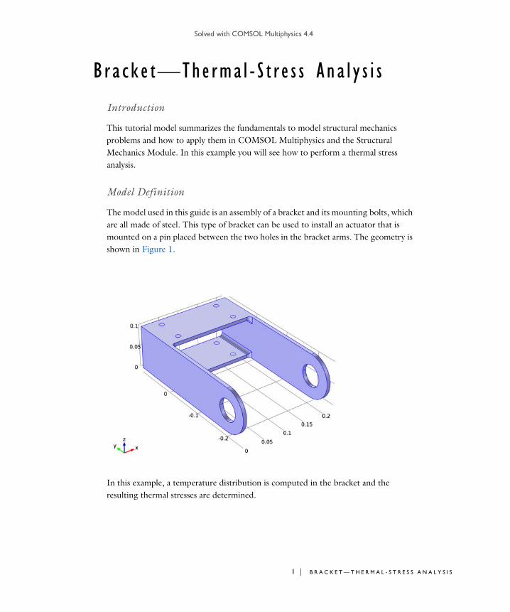
Solved with COMSOL Multiphysics 4.4
B r a c k e t—The rma l - S t r e s s Ana l y s i s
Introduction
This tutorial model summarizes the fundamentals to model structural mechanics problems and how to apply them in COMSOL Multiphysics and the Structural Mechanics Module. In this example you will see how to perform a thermal stress analysis.
Model Definition
The model used in this guide is an assembly of a bracket and its mounting bolts, which are all made of steel. This type of bracket can be used to install an actuator that is mounted on a pin placed between the two holes in the bracket arms. The geometry is shown in Figure 1.
In this example, a temperature distribution is computed in the bracket and the resulting thermal stresses are determined.
1 | B R A C K E T — T H E R M A L - S T R E S S A N A L Y S I S

Solved with COMSOL Multiphysics 4.4
2 | B R A
Results
Figure 1shows the temperature distribution in the bracket.
Figure 1: Temperature distribution in the bracket.
Figure 2shows the von Mises stress distribution in the bracket. You can see how the bracket arms holding the pin are deformed through thermal expansion and that thermal stresses have developed.
C K E T — T H E R M A L - S T R E S S A N A L Y S I S

Solved with COMSOL Multiphysics 4.4
Figure 2: Von Mises stress distribution in the bracket.
Notes About the COMSOL Implementation
COMSOL Multiphysics contains physics interfaces for structural analysis as well as thermal analysis. You can set up the coupled analysis for thermal-structure interaction using three different methods:
1 Add a Thermal Stress interface as in this example. The coupling is predefined and appears in the Thermal Expansion and Temperature Coupling nodes under Multiphysics. This is the easiest approach.
2 Add separate Solid Mechanics and Thermal Stress interfaces. Then add Thermal
Expansion and Temperature Coupling nodes under Multiphysics, and check the settings in them.
3 Add separate Solid Mechanics and Thermal Stress interfaces. Add a Thermal Expansion subnode under Linear Elastic Material, and do the appropriate settings there.
Model Library path: Structural_Mechanics_Module/Tutorial_Models/bracket_thermal
3 | B R A C K E T — T H E R M A L - S T R E S S A N A L Y S I S

Solved with COMSOL Multiphysics 4.4
4 | B R A
Modeling Instructions
1 On the Home toolbar, click Model Library.
2 Go to the Model Library window. In the Model Library tree, select Structural Mechanics
Module>Tutorial Models>bracket basic.
3 Click Open Model.
C O M P O N E N T 1
1 On the Home toolbar, click Add Physics.
A D D P H Y S I C S
1 Go to the Add Physics window.
2 In the Add Physics tree, select Structural Mechanics>Thermal Stress.
3 In the Add Physics window, click Add to Component.
4 On the Home toolbar, click Add Physics to close the Add Physics window.
R O O T
On the Home toolbar, click Add Study.
A D D S T U D Y
1 Go to the Add Study window.
2 Find the Studies subsection. In the tree, select Preset Studies>Stationary.
3 In the Add study window, click Add Study.
4 On the Home toolbar, click Add Study to close the Add Study window.
M U L T I P H Y S I C S
The thermal expansion requires both a thermal expansion coefficient and a strain reference temperature, which is the temperature reference at which there are no thermal strains. As a material (structural steel) has already been defined for the model, you do not need to modify anything in the Thermal Expansion node under Multiphysics.
S O L I D M E C H A N I C S
Fixed Constraint 11 On the Physics toolbar, click Domains and choose Fixed Constraint.
2 In the Fixed Constraint settings window, locate the Domain Selection section.
3 From the Selection list, choose Box 1.
C K E T — T H E R M A L - S T R E S S A N A L Y S I S

Solved with COMSOL Multiphysics 4.4
H E A T TR A N S F E R I N S O L I D S ( H T )
As the Heat Transfer in Solids interface includes a heat balance, the thermal boundary conditions also must also be set. Assume that heat is lost by convection to the surroundings from the surfaces of the arms and the bolt support.
Temperature 11 On the Physics toolbar, click Boundaries and choose Temperature.
Assume that the mounting bolts are kept at a temperature of 20oC .
2 Select Boundaries 22, 25, 30, 33, 46, 49, 54, and 57 only.
Temperature 21 On the Physics toolbar, click Boundaries and choose Temperature.
Assume that the arms of the bracket are holding the pin, which itself has a constant temperature of 100oC .
2 In the Temperature settings window, locate the Boundary Selection section.
3 From the Selection list, choose Box 2.
4 Locate the Temperature section. In the T0 edit field, type 100[degC].
Heat Flux 11 On the Physics toolbar, click Boundaries and choose Heat Flux.
2 In the Heat Flux settings window, locate the Heat Flux section.
3 Click the Inward heat flux button.
4 Locate the Boundary Selection section. From the Selection list, choose All boundaries.
5 Locate the Heat Flux section. In the h edit field, type 10.
S T U D Y 1
On the Home toolbar, click Compute.
R E S U L T S
Stress Under the Results node, three plot groups are automatically added to show the default results for a structural analysis and a thermal analysis. The first plot group, Stress, shows the von Mises stresses on the deformed geometry.
5 | B R A C K E T — T H E R M A L - S T R E S S A N A L Y S I S

Solved with COMSOL Multiphysics 4.4
6 | B R A
C K E T — T H E R M A L - S T R E S S A N A L Y S I S
Solved with COMSOL Multiphysics 4.4
B r a c k e t—Tran s i e n t Ana l y s i s
Introduction
Transient analyses provide the time domain response of a structure subjected to time-dependent loads. A transient analysis can be important when the time scale of the load is such that inertial or damping effects might have a significant influence on the behavior of the structure.
In this example you learn how to add damping properties to the material, define external loads varying with time, set up time-stepping data for the study, and generate animations.
It is recommended you review the Introduction to the Structural Mechanics Module, which includes background information and discusses the bracket_basic.mph models relevant to this example.
Model Definition
This model is an extension to the model example described in the section “The Fundamentals: A Static Linear Analysis” in the Introduction to the Structural Mechanics Module.
The model geometry is represented in Figure 1.
1 | B R A C K E T — TR A N S I E N T A N A L Y S I S

Solved with COMSOL Multiphysics 4.4
2 | B R A
Figure 1: Bracket geometry.
A rigid body is assumed to be connected to the arms of the bracket on which the time-varying load is applied.
C K E T — TR A N S I E N T A N A L Y S I S

Solved with COMSOL Multiphysics 4.4
Results and Discussion
Figure 2 shows the rigid connector’s displacements at the center of rotation versus the time.
Figure 2: Displacement of the pin center of rotation vs time.
Notes About the COMSOL Implementation
To accurately model the physical problem, you need to apply damping in a dynamic analysis. In COMSOL you have the possibility to add damping of several type: isotropic loss factor, anisotropic loss factor or Rayleigh damping.
To implement time-dependent components you can enter expressions using the variable t, the time variable in COMSOL Multiphysics.
The scaling of the displacement variables can be changed to correspond to the expected deformations. Manual scaling is the default for the displacement variables. The default manual scaling used for the structural displacement is 1/100th of the geometry size, which in this example is about 200 mm. In this case the expected deformations are in the order of 0.1 mm. The manual scaling factor should thus be changed to 10-4.
3 | B R A C K E T — TR A N S I E N T A N A L Y S I S

Solved with COMSOL Multiphysics 4.4
4 | B R A
Model Library path: Structural_Mechanics_Module/Tutorial_Models/bracket_transient
Modeling Instructions
1 On the Home toolbar, click Model Library.
2 Go to the Model Library window. In the Model Library tree, select Structural Mechanics
Module>Tutorial Models>bracket basic.
3 Click Open Model.
C O M P O N E N T 1
1 On the Home toolbar, click Add Physics.
A D D P H Y S I C S
1 Go to the Add Physics window.
2 In the Add physics tree, select Structural Mechanics>Solid Mechanics.
3 In the Add physics window, click Add to Component.
R O O T
On the Home toolbar, click Add Study.
A D D S T U D Y
1 Go to the Add Study window.
2 Find the Studies subsection. In the tree, select Preset Studies>Time Dependent.
3 In the Add study window, click Add Study.
S O L I D M E C H A N I C S
Damping 11 In the Model Builder window, under Component 1 >Solid Mechanics right-click Linear
Elastic Material 1 and choose Damping.
In this example, you will use Rayleigh damping.
2 In the Damping settings window, locate the Damping Settings section.
3 In the dM edit field, type 100.
4 In the dK edit field, type 3e-4.
C K E T — TR A N S I E N T A N A L Y S I S

Solved with COMSOL Multiphysics 4.4
Fixed Constraint 11 On the Physics toolbar, click Domains and choose Fixed Constraint.
2 In the Fixed Constraint settings window, locate the Domain Selection section.
3 From the Selection list, choose Box 1.
To represent the pin between the arms of the bracket you can use a rigid connector, to which a load can be applied.
Rigid Connector 11 On the Physics toolbar, click Boundaries and choose Rigid Connector.
2 In the Rigid Connector settings window, locate the Boundary Selection section.
3 From the Selection list, choose Box 2.
Applied Force 11 Right-click Component 1 >Solid Mechanics >Rigid Connector 1 and choose Applied
Force.
2 In the Applied Force settings window, locate the Applied Force section.
3 Specify the F vector as
S T U D Y 1
Step 1: Time Dependent1 In the Model Builder window, expand the Study 1 node, then click Step 1: Time
Dependent.
2 In the Time Dependent settings window, locate the Study Settings section.
3 From the Time unit list, choose ms.
4 In the Times edit field, type range(0,0.25,15).
With this time stepping, the solver automatically stores the solution every 0.25 ms from 0 to 15 ms.
The time-dependent solver adapts its time stepping based on a tolerance criterion. This ensures that the solver takes small enough time steps if large variations occur between the specified output times.
5 Select the Relative tolerance check box.
1e3*sin(2*pi*t*200[1/s]) x
-1e5 y
1e4*sin(2*pi*t*100[1/s]) z
5 | B R A C K E T — TR A N S I E N T A N A L Y S I S

Solved with COMSOL Multiphysics 4.4
6 | B R A
6 In the associated edit field, type 0.001.
7 Click to expand the Results while solving section. Select the Plot check box.
Solver 11 On the Study toolbar, click Show Default Solver.
2 In the Model Builder window, expand the Study 1>Solver Configurations>Solver
1>Dependent Variables 1 node, then click Displacement field (Material) (comp1.u).
3 In the Field settings window, locate the Scaling section.
4 In the Scale edit field, type 1e-4.
The computation can be accelerated for a small model by disabling the convergence plot. To do this, go to the File menu and select Preferences. Under Results, click to clear the Generate convergence plots check box.
5 On the Home toolbar, click Compute.
R E S U L T S
StressThe default plot shows the stress distribution at the final time. You can change the time for the plot display in the Time list of the plot group's Settings window.
An alternative is to create a player.
Export1 Click the Player button on the Results toolbar.
COMSOL Multiphysics generates the movie and then plays it. To replay the movie, click the Play button on the Graphics toolbar.
If you want to export a movie in GIF, Flash, or AVI format, right-click Export and create an Animation feature.
Plot the displacement of the center of rotation of the rigid body versus the time.
1D Plot Group 21 On the Home toolbar, click Add Plot Group and choose 1D Plot Group.
2 In the 1D Plot Group settings window, click to expand the Title section.
3 From the Title type list, choose Manual.
4 In the Title text area, type Pin center of rotation displacement.
5 Click to expand the Legend section. From the Position list, choose Upper left.
6 On the 1D Plot Group 2 toolbar, click Global.
C K E T — TR A N S I E N T A N A L Y S I S

Solved with COMSOL Multiphysics 4.4
7 In the Global settings window, locate the y-Axis Data section.
8 Click Add Expression in the upper-right corner of the y-Axis Data section. From the menu choose Solid Mechanics>Rigid body displacement, x component (solid.rig1.u). In the table, enter the following settings:
9 Click Add Expression in the upper-right corner of the y-Axis Data section. From the menu choose Solid Mechanics>Rigid body displacement, y component (solid.rig1.v). In the table, enter the following settings:
10 Click Add Expression in the upper-right corner of the y-Axis Data section. From the menu choose Solid Mechanics>Rigid body displacement, z component (solid.rig1.w). In the table, enter the following settings:
11 On the 1D Plot Group 2 toolbar, click Plot.
Expression Unit Description
solid.rig1.u m x-component
Expression Unit Description
solid.rig1.v m y-component
Expression Unit Description
solid.rig1.w m z-component
7 | B R A C K E T — TR A N S I E N T A N A L Y S I S

Solved with COMSOL Multiphysics 4.4
8 | B R A
C K E T — TR A N S I E N T A N A L Y S I S
Solved with COMSOL Multiphysics 4.4
V i b r a t i o n s o f a D i s k Ba c k ed b y an A i r - F i l l e d C y l i n d e r
Introduction
The vibration modes of a thin or thick circular disc are well known, and it is possible to compute the corresponding eigenfrequencies with an arbitrary precision from a series solution. The same is true for the acoustic modes of an air-filled cylinder with perfectly rigid walls. A more interesting question to ask is: What happens if the cylinder is sealed in one end not by a rigid wall but by a thin disc? This is the question you address in this model.
This model uses the Structural Mechanics Module’s Shell interface and the Pressure Acoustics interface from COMSOL Multiphysics. If you have a license for the Acoustics Module, see Vibrations of a Disk Backed by an Air-Filled Cylinder in the Acoustics Module Model Library for a model version that uses the Acoustic-Shell Interaction multiphysics interface.
Model Definition
The geometry is a rigid steel cylinder with a height of 255 mm and a radius of 38 mm. One end is welded to a heavy slab, while the other is sealed with a steel disc only 0.38 mm thick. The disc is modeled using shell elements with the outer edge of the disc fixed. The acoustics in the cylinder is described in terms of the acoustic (differential) pressure. The eigenvalue equation for the pressure is
where c is the speed of sound and 2f defines the eigenfrequency, f.
A first step is to calculate the eigenfrequencies for the disc and the cylinder separately and compare them with theoretical values. This way you can verify the basic components of the model and assess the accuracy of the finite-element solution before modeling the coupled system. In a second step you simulate a decoupled problem, where the acoustic domain is completely surrounded by sound hard boundaries. In the third step you perform a coupled analysis where the boundary at the disc will instead
p–2
c2------ p=
1 | V I B R A T I O N S O F A D I S K B A C K E D B Y A N A I R - F I L L E D C Y L I N D E R

Solved with COMSOL Multiphysics 4.4
2 | V I B R
have the accelerations of the disc as boundary conditions. At the same time, the acoustic pressure supplies a load on the disc.
Results and Discussion
In Ref. 1, D.G. Gorman and others have thoroughly investigated the model at hand, and they have developed a semi-analytical solution verified by experiments and simulations. Some of the theoretical eigenfrequencies of a thin disc in vacuum and of a rigidly sealed chamber are given in Table 1. The difference between theoretical and computed values are below 1% for all modes.
Figure 1 through Figure 4 show the two first uncoupled structural and acoustic modes.
A T I O N S O F A D I S K B A C K E D B Y A N A I R - F I L L E D C Y L I N D E R

Solved with COMSOL Multiphysics 4.4
Figure 1: First structural mode represented with vertical displacement.
Figure 2: Second structural mode represented with vertical displacement.
3 | V I B R A T I O N S O F A D I S K B A C K E D B Y A N A I R - F I L L E D C Y L I N D E R

Solved with COMSOL Multiphysics 4.4
4 | V I B R
Figure 3: First acoustic mode represented with pressure isosurfaces.
Figure 4: Second acoustic mode represented with pressure isosurfaces.
A T I O N S O F A D I S K B A C K E D B Y A N A I R - F I L L E D C Y L I N D E R

Solved with COMSOL Multiphysics 4.4
All structurally dominated (str), acoustically dominated (ac), or tightly coupled (str/ac) modes are shown in Table 1 that compares the eigenfrequencies from the COMSOL Multiphysics analysis with the semi-analytical and experimental frequencies reported in Ref. 1. Most of the modes show rather weak coupling between the structural bending of the disc and the pressure field in the cylinder. It is, however, interesting to note that some of the uncoupled modes have been split into one covibrating and one contravibrating mode with distinct eigenfrequencies. This is the case for modes 1 and 2 and for modes 9 and 11 in the list below. Due to symmetry the pure structural analysis has 2 eigenmodes for each eigenfrequency, as show in the table.
As the table shows, the FEM solution is in good agreement with both the theoretical predictions and the experimentally measured values for the eigenfrequencies. As you might expect from the evaluation of the accuracies for the uncoupled problems, the precision is generally better for the acoustics-dominated modes.
In Figure 5 the first coupled mode is shown in terms of disc displacements and air pressure. The coupling effect can be clearly displayed using a plot of pressure gradients, as in Figure 6.
TABLE 1: RESULTS FROM SEMI-ANALYTICAL AND COMSOL MULTIPHYSICS ANALYSES AND EXPERIMENTAL DATA
Type Semi-analytical (Hz) COMSOL Multiphysics (Hz) Experimental (Hz)
str/ac 636.9 637.1 630
str/ac 707.7 707.6 685
ac 1347 1347 1348
str 1394 1394/1395 1376
ac 2018 2018 2040
str 2289 2291/2294 2170
str/ac 2607 2618 2596
ac 2645 2646 –
str/ac 2697 2697 2689
ac 2730 2730 2756
ac 2968 2968 2971
5 | V I B R A T I O N S O F A D I S K B A C K E D B Y A N A I R - F I L L E D C Y L I N D E R

Solved with COMSOL Multiphysics 4.4
6 | V I B R
Figure 5: Disc deformation and pressure contours for the first coupled mode.
Figure 6: Disc deformation and pressure gradient contours for the first coupled mode.
A T I O N S O F A D I S K B A C K E D B Y A N A I R - F I L L E D C Y L I N D E R

Solved with COMSOL Multiphysics 4.4
Reference
1. D.G. Gorman, J.M. Reese, J. Horacek, and D. Dedouch, “Vibration Analysis of a Circular Disk Backed by a Cylindrical Cavity,” Proc. Instn. Mech. Engrs., vol. 215, Part C, 2001.
Notes About the COMSOL Implementation
You specify the part of the physics for which to compute the uncoupled eigenvalues by selecting the variables for the eigenvalue solver.
When coupling the two types of physics, be careful when selecting the sign of the coupling terms, so that they act in the intended direction. You should specify the acceleration in the inward normal direction for the pressure acoustics domain, which in this case is the positive z acceleration of the disc. The variable wtt, it is the second time-derivative of the variable w. The pressure on the shell can be given using global directions, so that a positive pressure acts as a face load in the negative z direction.
Model Library path: Structural_Mechanics_Module/Acoustic-Structure_Interaction/coupled_vibrations
Modeling Instructions
From the File menu, choose New.
N E W
1 In the New window, click the Model Wizard button.
M O D E L W I Z A R D
1 In the Model Wizard window, click the 3D button.
2 In the Select Physics tree, select Structural Mechanics>Shell (shell).
3 Click the Add button.
4 In the Select Physics tree, select Acoustics>Pressure Acoustics>Pressure Acoustics,
Frequency Domain (acpr).
5 Click the Add button.
6 Click the Study button.
7 | V I B R A T I O N S O F A D I S K B A C K E D B Y A N A I R - F I L L E D C Y L I N D E R

Solved with COMSOL Multiphysics 4.4
8 | V I B R
7 In the tree, select Preset Studies for Selected Physics>Eigenfrequency.
8 Click the Done button.
S T U D Y 1
Step 1: EigenfrequencyIn the first study, you solve the structural problem only. Exclude the Pressure Acoustics interface.
1 In the Model Builder window, under Study 1 click Step 1: Eigenfrequency.
2 In the Eigenfrequency settings window, locate the Physics and Variables Selection section.
3 In the table, enter the following settings:
G E O M E T R Y 1
Cylinder 11 On the Geometry toolbar, click Cylinder.
2 In the Cylinder settings window, locate the Size and Shape section.
3 In the Radius edit field, type 0.038.
4 In the Height edit field, type 0.255.
5 Click the Build Selected button.
Form UnionIn the Model Builder window, under Component 1>Geometry 1 right-click Form Union and choose Build Selected.
S H E L L
1 In the Model Builder window, under Component 1 click Shell.
2 Select Boundary 3 only.
3 In the Shell settings window, locate the Thickness section.
4 In the d edit field, type 0.00038.
Fixed Constraint 11 On the Physics toolbar, click Edges and choose Fixed Constraint.
2 Select Edges 2, 3, 7, and 10 only.
Physics Solve for Discretization
Pressure Acoustics, Frequency Domain × Physics settings
A T I O N S O F A D I S K B A C K E D B Y A N A I R - F I L L E D C Y L I N D E R

Solved with COMSOL Multiphysics 4.4
M A T E R I A L S
Material 11 In the Model Builder window, under Component 1 right-click Materials and choose
New Material.
2 In the Material settings window, locate the Material Contents section.
3 In the table, enter the following settings:
Material 21 In the Model Builder window, right-click Materials and choose New Material.
2 In the Material settings window, locate the Geometric Entity Selection section.
3 From the Geometric entity level list, choose Boundary.
4 Select Boundary 3 only.
5 Locate the Material Contents section. In the table, enter the following settings:
M E S H 1
Free Quad 11 In the Model Builder window, under Component 1 right-click Mesh 1 and choose More
Operations>Free Quad.
2 Select Boundary 3 only.
Size1 In the Model Builder window, under Component 1>Mesh 1 click Size.
2 In the Size settings window, locate the Element Size section.
3 Click the Custom button.
4 Locate the Element Size Parameters section. In the Maximum element size edit field, type 0.01.
Property Name Value Unit Property group
Density rho 1.2 kg/m³ Basic
Speed of sound c 343 m/s Basic
Property Name Value Unit Property group
Young's modulus E 2.1e11 Pa Basic
Poisson's ratio nu 0.3 1 Basic
Density rho 7800 kg/m³ Basic
9 | V I B R A T I O N S O F A D I S K B A C K E D B Y A N A I R - F I L L E D C Y L I N D E R

Solved with COMSOL Multiphysics 4.4
10 | V I B
Free Quad 1In the Model Builder window, under Component 1>Mesh 1 right-click Free Quad 1 and choose Build Selected.
Swept 11 Right-click Mesh 1 and choose Swept.
2 In the Model Builder window, under Component 1>Mesh 1 right-click Swept 1 and choose Build Selected.
S T U D Y 1
Step 1: Eigenfrequency1 In the Model Builder window, expand the Study 1 node, then click Step 1:
Eigenfrequency.
2 In the Eigenfrequency settings window, locate the Study Settings section.
3 In the Desired number of eigenfrequencies edit field, type 20.
4 In the Search for eigenfrequencies around edit field, type 500.
5 On the Home toolbar, click Compute.
R E S U L T S
Mode Shape (shell)1 In the Model Builder window, expand the Mode Shape (shell) node, then click Surface
1.
2 In the Surface settings window, click Replace Expression in the upper-right corner of the Expression section. From the menu, choose Shell>Displacement>Displacement
field>Displacement field, z component (w).
3 On the Mode Shape (shell) toolbar, click Plot.
4 Click the Go to XY View button on the Graphics toolbar.
5 In the Model Builder window, click Mode Shape (shell).
6 In the 3D Plot Group settings window, locate the Data section.
7 From the Eigenfrequency list, choose 1398.666818.
8 On the Mode Shape (shell) toolbar, click Plot.
R O O T
Add the second study to solve the pure acoustics problem.
1 On the Home toolbar, click Add Study.
R A T I O N S O F A D I S K B A C K E D B Y A N A I R - F I L L E D C Y L I N D E R

Solved with COMSOL Multiphysics 4.4
A D D S T U D Y
For this study, exclude the Shell interface.
1 Go to the Add Study window.
2 Find the Studies subsection. In the tree, select Preset Studies>Eigenfrequency.
3 Find the Physics in study subsection. In the table, enter the following settings:
4 In the Add study window, click Add Study.
5 On the Home toolbar, click Add Study.
S T U D Y 2
Step 1: Eigenfrequency1 In the Model Builder window, under Study 2 click Step 1: Eigenfrequency.
2 In the Eigenfrequency settings window, locate the Study Settings section.
3 In the Desired number of eigenfrequencies edit field, type 20.
4 In the Search for eigenfrequencies around edit field, type 500.
5 On the Home toolbar, click Compute.
R E S U L T S
Acoustic Pressure, Isosurfaces (acpr)1 In the 3D Plot Group settings window, locate the Data section.
2 From the Eigenfrequency list, choose 672.549058.
3 In the Model Builder window, under Results>Acoustic Pressure, Isosurfaces (acpr) click Isosurface 1.
4 In the Isosurface settings window, locate the Coloring and Style section.
5 From the Color table list, choose WaveLight.
6 Select the Symmetrize color range check box.
7 On the Acoustic Pressure, Isosurfaces (acpr) toolbar, click Plot.
8 Click the Go to Default 3D View button on the Graphics toolbar.
9 In the Model Builder window, click Acoustic Pressure, Isosurfaces (acpr).
10 In the 3D Plot Group settings window, locate the Data section.
11 From the Eigenfrequency list, choose 1345.101094.
Physics Solve
Shell (shell) ×
11 | V I B R A T I O N S O F A D I S K B A C K E D B Y A N A I R - F I L L E D C Y L I N D E R

Solved with COMSOL Multiphysics 4.4
12 | V I B
12 On the Acoustic Pressure, Isosurfaces (acpr) toolbar, click Plot.
Add the boundary conditions that couple the Pressure Acoustics and Shell interfaces.
S H E L L
Face Load 11 On the Physics toolbar, click Boundaries and choose Face Load.
2 Select Boundary 3 only.
The acoustic pressure exerts a normal load on the plate. Thus, set the z-component of the load per unit area equal to -p.
3 In the Face Load settings window, locate the Force section.
4 Specify the FA vector as
P R E S S U R E A C O U S T I C S , F R E Q U E N C Y D O M A I N
Normal Acceleration 11 On the Physics toolbar, click Boundaries and choose Normal Acceleration.
2 Select Boundary 3 only.
The inward normal acceleration at the plate equals the second time derivative of the vertical displacemen.
3 In the Normal Acceleration settings window, locate the Normal Acceleration section.
4 In the an edit field, type wtt.
Add the third study for the coupled problem.
R O O T
On the Home toolbar, click Add Study.
A D D S T U D Y
1 Go to the Add Study window.
2 Find the Studies subsection. In the tree, select Preset Studies>Eigenfrequency.
3 In the Add study window, click Add Study.
4 On the Home toolbar, click Add Study.
0 x
0 y
-p z
R A T I O N S O F A D I S K B A C K E D B Y A N A I R - F I L L E D C Y L I N D E R

Solved with COMSOL Multiphysics 4.4
S T U D Y 3
Step 1: Eigenfrequency1 In the Model Builder window, under Study 3 click Step 1: Eigenfrequency.
2 In the Eigenfrequency settings window, locate the Study Settings section.
3 In the Desired number of eigenfrequencies edit field, type 20.
4 In the Search for eigenfrequencies around edit field, type 500.
5 On the Home toolbar, click Compute.
R E S U L T S
Mode Shape (shell) 11 In the Model Builder window, click Mode Shape (shell) 1.
2 In the 3D Plot Group settings window, locate the Data section.
3 From the Eigenfrequency list, choose 637.052763.
4 In the Model Builder window, expand the Mode Shape (shell) 1 node, then click Surface
1.
5 In the Surface settings window, click Replace Expression in the upper-right corner of the Expression section. From the menu, choose Displacement field, z component (w).
6 In the Model Builder window, right-click Mode Shape (shell) 1 and choose Slice.
7 In the Slice settings window, locate the Plane Data section.
8 In the Planes edit field, type 1.
9 Locate the Coloring and Style section. From the Color table list, choose WaveLight.
10 On the Mode Shape (shell) 1 toolbar, click Plot.
11 Click the Zoom Extents button on the Graphics toolbar.
Plot the pressure gradient to display the connection to the disk shape.
12 Locate the Expression section. In the Expression edit field, type pz.
13 From the Unit list, choose Pa/m.
14 On the Mode Shape (shell) 1 toolbar, click Plot.
13 | V I B R A T I O N S O F A D I S K B A C K E D B Y A N A I R - F I L L E D C Y L I N D E R

Solved with COMSOL Multiphysics 4.4
14 | V I B
R A T I O N S O F A D I S K B A C K E D B Y A N A I R - F I L L E D C Y L I N D E R
Solved with COMSOL Multiphysics 4.4
S t a t i c and E i g e n f r e qu en c y Ana l y s e s o f an E l b ow B r a c k e t
Introduction
The component depicted in Figure 1 is part of a support mechanism and is subjected to both mechanical loads and thermal loads. This tutorial model takes you through the steps to carry out a detailed analysis of the part using the Structural Mechanics Module.
Figure 1: Geometry of the elbow bracket.
In the various parts of the example you are introduced to using the available basic analysis types, together with numerous postprocessing possibilities. These analysis types are:
• Static analysis
• Eigenfrequency analysis
• Damped eigenfrequency analysis
• Transient analysis
• Modal based transient analysis
• Frequency response analysis
• Modal based frequency response analysis
• Parametric analysis
• Linear buckling analysis
1 | S T A T I C A N D E I G E N F R E Q U E N C Y A N A L Y S E S O F A N E L B O W B R A C K E T

Solved with COMSOL Multiphysics 4.4
2 | S T A
This tutorial model comes in two versions:
• A short version, elbow_bracket_brief, treating the three first analysis types in the above list.
• A complete version, elbow_bracket, treating all nine analysis types.
Each of the listed analysis types corresponds to a study type; the available studies are described in the section Available Study Types in the Structural Mechanics Module User’s Guide. The chapter Structural Mechanics Modeling in the same manual provides further assistance.
Model Definition
The geometry for this part, see Figure 1, has been created with a CAD software, and it is available for you to import into COMSOL Multiphysics.
MaterialStructural steel, as taken from the material library, with Young’s modulus of 200 GPa, Poisson’s ratio of 0.33, and coefficient of thermal expansion 12.3·10-6 K1.
DampingThe Structural Mechanics Module supports Rayleigh damping and loss factor damping. You can also use no damping, which is the default option.
In some of the analyses here you will use Rayleigh damping, where you specify damping parameters that are proportional to the mass (dM) and stiffness (dK) in the following way:
where C is the damping matrix, M is the mass matrix, and K is the stiffness matrix. The damping is specified locally in each domain; this means that you can specify different damping parameters in different parts of the model.
To find the values for the Rayleigh damping, you can use the relations between the critical damping ratio and the Rayleigh damping parameters. It is often easier to interpret the critical damping ratios, which are given by
C dMM dKK+=
i
dM
i----------- dK i+
2--------------------------------------------=
T I C A N D E I G E N F R E Q U E N C Y A N A L Y S E S O F A N E L B O W B R A C K E T

Solved with COMSOL Multiphysics 4.4
where i is the critical damping ratio at a specific angular frequency i. Knowing two pairs of corresponding i and i results in a system of equations
with the damping parameters as the unknown variables.
Assume that the structure has a constant damping ratio of 0.1. Select two frequencies near the excitation frequency, 400 Hz and 600 Hz. Solving the system of equations above will give the result is dM = 300 and dK = 3.2·105.
For more information see the section Modeling Damping and Losses in the Structural Mechanics Module User’s Guide.
If modal-based dynamic response studies are performed it is usually easier to give the critical damping ratios directly. This will also give more detailed control over the damping properties over a large frequency range.
Loads and ConstraintsThe displacement are fixed in all directions on the face shown in Figure 2. The load is described under each study, but in all cases it is distributed over the face shown in this figure.
Figure 2: Constraint and loading of the bracket.
12 1
-------------------12
------
12 2
-------------------22
------
dM
dK
1
2
=
Loaded face
Fixed face
3 | S T A T I C A N D E I G E N F R E Q U E N C Y A N A L Y S E S O F A N E L B O W B R A C K E T

Solved with COMSOL Multiphysics 4.4
4 | S T A
The Model Library note immediately below appears in the discussion of every model. The path indicates the location of the model file in the Model Library root directory. The most convenient way to open it is from the Model Library window in the COMSOL Desktop, which you can open from the File menu.
Model Library path: Structural_Mechanics_Module/Tutorial_Models/elbow_bracket_brief
Modeling Instructions
From the File menu, choose New.
N E W
1 In the New window, click the Model Wizard button.
M O D E L W I Z A R D
1 In the Model Wizard window under Select Space Dimension, click the 3D button.
2 In the Select physics tree, select Structural Mechanics>Solid Mechanics.
3 Click the Add button.
4 Click the Study button.
5 In the tree, select Preset Studies>Stationary.
6 Click the Done button.
G E O M E T R Y 1
Import 11 On the Home toolbar, click Import.
2 In the Import settings window, locate the Import section.
3 From the Geometry import list, choose COMSOL Multiphysics file.
4 Click the Browse button.
5 Browse to the model’s Model Library folder and double-click the file elbow_bracket.mphbin.
6 Click the Import button.
T I C A N D E I G E N F R E Q U E N C Y A N A L Y S E S O F A N E L B O W B R A C K E T

Solved with COMSOL Multiphysics 4.4
7 Click the Wireframe Rendering button on the Graphics toolbar.
The view in the Graphics window should look like that in the image below.
8 Click the Wireframe Rendering button on the Graphics toolbar to return to the default surface rendering.
Suppress some edges during meshing, in order to avoid generation of unnecessary small elements.
Ignore Edges 11 On the Geometry toolbar, click Virtual Operations and choose Ignore Edges.
2 On the object fin, select Edges 17, 21, 23, 27, 38, 40, 42, and 44 only.
M E S H 1
Size1 In the Model Builder window, under Component 1 right-click Mesh 1 and choose Free
Tetrahedral.
The default free mesher has nine predefined combinations of mesh parameter settings. They range from Extremely fine to Extremely coarse, with Normal as the default setting. Unless any other mesh parameters are set, this is the setting that is used if you use Build All or Build Selected to generate the mesh.
2 In the Size settings window, locate the Element Size section.
3 From the Predefined list, choose Coarse.
5 | S T A T I C A N D E I G E N F R E Q U E N C Y A N A L Y S E S O F A N E L B O W B R A C K E T

Solved with COMSOL Multiphysics 4.4
6 | S T A
As a stress concentration can be expected in the corner of the bracket, put a finer mesh there.
Size 11 In the Model Builder window, under Component 1 >Mesh 1 right-click Free Tetrahedral
1 and choose Size.
2 In the Size settings window, locate the Geometric Entity Selection section.
3 From the Geometric entity level list, choose Boundary.
4 Locate the Element Size section. From the Predefined list, choose Finer.
5 Select Boundaries 13 and 14 only.
Size 21 Right-click Free Tetrahedral 1 and choose Size.
2 In the Size settings window, locate the Geometric Entity Selection section.
3 From the Geometric entity level list, choose Edge.
4 Select Edges 25 and 48 only.
5 Locate the Element Size section. From the Predefined list, choose Extra fine.
6 In the Model Builder window, right-click Mesh 1 and choose Build All.
M A T E R I A L S
Next, specify the material properties. You can do this either by explicitly typing them in or by selecting a library material in the Material Browser. For this model, use a library material.
1 On the Home toolbar, click Add Material.
A D D M A T E R I A L
1 Go to the Add Material window.
2 In the tree, select Built-In>Structural steel.
3 In the Add material window, click Add to Component.
4 On the Home toolbar, click Add Material.
Static Analysis
A static analysis has no explicit or implicit time dependencies. This situation corresponds to the steady state with constant (in time) boundary conditions and material properties.
T I C A N D E I G E N F R E Q U E N C Y A N A L Y S E S O F A N E L B O W B R A C K E T

Solved with COMSOL Multiphysics 4.4
The purpose of such analysis can be to find the maximum stress level and compare it with the material’s yield strength, as well as to check that the deformation of the component is within the limits of the design criteria.
Results and Discussion
The analysis shows that the von Mises effective stress has a maximum value of about190 MPa, which, compared with the material’s yield strength of 350 MPa, results in a utilization factor of 54%.
The analysis also gives the maximum static displacements as 1.14 mm
Three different representations of the stress state are shown in Figure 3 through Figure 5.
Figure 3: Effective stresses on the boundary of the domain.
7 | S T A T I C A N D E I G E N F R E Q U E N C Y A N A L Y S E S O F A N E L B O W B R A C K E T

Solved with COMSOL Multiphysics 4.4
8 | S T A
Figure 4: Isosurface plot of the effective stress.
Figure 5: Arrow plot of the principal stresses.
T I C A N D E I G E N F R E Q U E N C Y A N A L Y S E S O F A N E L B O W B R A C K E T

Solved with COMSOL Multiphysics 4.4
Modeling Instructions
S O L I D M E C H A N I C S
Fixed Constraint 11 On the Physics toolbar, click Boundaries and choose Fixed Constraint.
2 Select Boundary 1 only.
Boundary Load 11 On the Physics toolbar, click Boundaries and choose Boundary Load.
2 Select Boundary 21 only.
3 In the Boundary Load settings window, locate the Force section.
4 Specify the FA vector as
S T U D Y 1
In this model, where there are many different studies, it is a good idea to assign manual names to some nodes in the model tree.
1 In the Model Builder window, right-click Study 1 and choose Rename.
2 Go to the Rename Study dialog box and type Study 1 in the New name edit field.
3 Click OK.
The default settings in the generated solver are OK for this model, so it can be run directly.
4 On the Home toolbar, click Compute.
Before moving on to analyzing the solution, rename the solver.
S T U D Y 1
In the Model Builder window, expand the Study 1 node.
Solver 11 In the Model Builder window, expand the Study 1>Solver Configurations node.
2 Right-click Solver 1 and choose Rename.
3[MPa] x
0 y
3[MPa] z
9 | S T A T I C A N D E I G E N F R E Q U E N C Y A N A L Y S E S O F A N E L B O W B R A C K E T

Solved with COMSOL Multiphysics 4.4
10 | S T
3 Go to the Rename Solver dialog box and type Solver, Static in the New name edit field.
4 Click OK.
R E S U L T S
Similarly, rename the solution data set.
Data Sets1 In the Model Builder window, under Results>Data Sets right-click Solution 1 and
choose Rename.
2 Go to the Rename Solution dialog box and type Static Solution in the New name edit field.
3 Click OK.
In the Results branch, you can create various plot types, evaluate expressions, or animate the results. The result features can visualize any expression containing, for example, the solution variables, their derivatives, and the space coordinates. Many frequently used expressions are predefined as postprocessing variables, and they are directly available in the Expression section menus for the various plot types.
When the solver finishes, a default plot appears. It shows a surface plot of the von Mises stress with the deformed shape of the component. For future reference, you can rename it.
Stress1 In the Model Builder window, under Results right-click Stress and choose Rename.
2 Go to the Rename 3D Plot Group dialog box and type Static Stress Contour in the New name edit field.
3 Click OK.
4 Click the Zoom Extents button on the Graphics toolbar.
To evaluate the maximum displacement, use a Maximum coupling operator.
D E F I N I T I O N S
Maximum 11 On the Definitions toolbar, click Component Couplings and choose Maximum.
2 In the Maximum settings window, locate the Source Selection section.
3 From the Geometric entity level list, choose Boundary.
A T I C A N D E I G E N F R E Q U E N C Y A N A L Y S E S O F A N E L B O W B R A C K E T

Solved with COMSOL Multiphysics 4.4
4 From the Selection list, choose All boundaries.
Variables 1a1 In the Model Builder window, right-click Definitions and choose Variables.
2 In the Variables settings window, locate the Variables section.
3 In the table, enter the following settings:
S T U D Y 1
Solver, StaticIn the Model Builder window, under Study 1>Solver Configurations right-click Solver,
Static and choose Solution>Update.
This step is necessary in order to access variables that were created after the solution was performed.
R E S U L T S
Derived Values1 On the Results toolbar, click Global Evaluation.
2 In the Global Evaluation settings window, click Replace Expression in the upper-right corner of the Expression section. From the menu, choose Definitions>Maximum
deflection.
3 Locate the Expression section. From the Unit list, choose mm.
4 Click the Evaluate button.
The result, approximately 1.1 mm appears in the Table window.
Next, add a second plot group and create an isosurface plot. The resulting plot should resemble that in Figure 4.
3D Plot Group 21 On the Home toolbar, click Add Plot Group and choose 3D Plot Group.
2 In the Model Builder window, under Results right-click 3D Plot Group 2 and choose Isosurface.
3 In the Isosurface settings window, click Replace Expression in the upper-right corner of the Expression section. From the menu, chooseSolid Mechanics>Stress>von Mises stress.
Name Expression Unit Description
U_max maxop1 m Maximum deflection
11 | S T A T I C A N D E I G E N F R E Q U E N C Y A N A L Y S E S O F A N E L B O W B R A C K E T

Solved with COMSOL Multiphysics 4.4
12 | S T
4 Right-click Results>3D Plot Group 2>Isosurface 1 and choose Deformation.
5 Right-click 3D Plot Group 2 and choose Rename.
6 Go to the Rename 3D Plot Group dialog box and type Static Stress Isosurface in the New name edit field.
7 Click OK.
8 Click the Go to Default 3D View button on the Graphics toolbar.
With the following steps you can reproduce the principal stress arrow plot shown in Figure 5:
3D Plot Group 31 On the Home toolbar, click Add Plot Group and choose 3D Plot Group.
2 On the 3D Plot Group 3 toolbar, click More Plots and choose Principal Stress Volume.
3 In the Principal Stress Volume settings window, locate the Positioning section.
4 In the X Grid Points edit field, type 10.
5 In the Y Grid Points edit field, type 15.
6 In the Z Grid Points edit field, type 10.
7 On the 3D Plot Group 3 toolbar, click Plot.
8 In the Model Builder window, right-click 3D Plot Group 3 and choose Rename.
9 Go to the Rename 3D Plot Group dialog box and type Static Principal Stress Arrow Plot in the New name edit field.
10 Click OK.
11 Click the Go to Default 3D View button on the Graphics toolbar.
Eigenfrequency Analysis
An eigenfrequency analysis finds the eigenfrequencies and modes of deformation of a component. The eigenfrequencies f in the structural mechanics field are related to the eigenvalues returned by the solvers through
(1)
In COMSOL Multiphysics you can choose between working with eigenfrequencies and working with eigenvalues according to your preferences. Eigenfrequencies is the default option for all physics interfaces in the Structural Mechanics Module.
f –2i---------=
A T I C A N D E I G E N F R E Q U E N C Y A N A L Y S E S O F A N E L B O W B R A C K E T
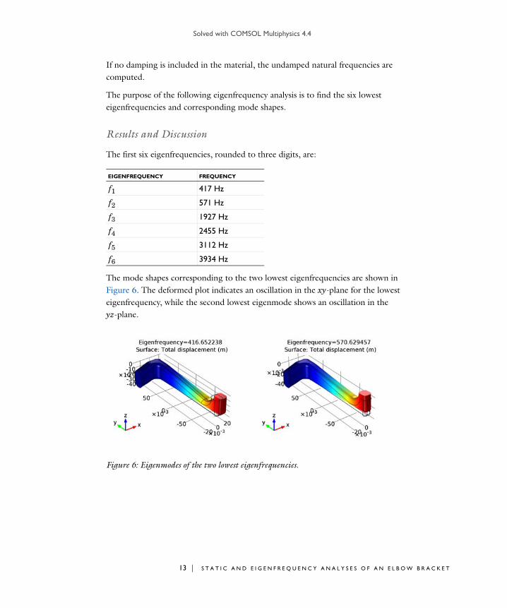
Solved with COMSOL Multiphysics 4.4
If no damping is included in the material, the undamped natural frequencies are computed.
The purpose of the following eigenfrequency analysis is to find the six lowest eigenfrequencies and corresponding mode shapes.
Results and Discussion
The first six eigenfrequencies, rounded to three digits, are:
The mode shapes corresponding to the two lowest eigenfrequencies are shown in Figure 6. The deformed plot indicates an oscillation in the xy-plane for the lowest eigenfrequency, while the second lowest eigenmode shows an oscillation in the yz-plane.
Figure 6: Eigenmodes of the two lowest eigenfrequencies.
EIGENFREQUENCY FREQUENCY
f1 417 Hz
f2 571 Hz
f3 1927 Hz
f4 2455 Hz
f5 3112 Hz
f6 3934 Hz
13 | S T A T I C A N D E I G E N F R E Q U E N C Y A N A L Y S E S O F A N E L B O W B R A C K E T

Solved with COMSOL Multiphysics 4.4
14 | S T
Notes About the COMSOL Implementation
Any loads present on the model, such as the load from the static load case above, are ignored in the default eigenfrequency analysis. It is also possible to include effects from prestress. You can find an example of such an analysis in the model Vibrating String.
Modeling Instructions
Add a new study to your model.
R O O T
On the Home toolbar, click Add Study.
A D D S T U D Y
1 Go to the Add Study window.
2 Find the Studies subsection. In the tree, select Preset Studies>Eigenfrequency.
3 In the Add Study window, click Add Study.
S T U D Y 2
1 In the Model Builder window, right-click Study 2 and choose Rename.
2 Go to the Rename Study dialog box and type Study 2 in the New name edit field.
3 Click OK.
4 On the Home toolbar, click Compute.
S T U D Y 2
Solver 21 In the Model Builder window, expand the Study 2>Solver Configurations node.
2 Right-click Solver 2 and choose Rename.
3 Go to the Rename Solver dialog box and type Solver, Eigenfrequency in the New
name edit field.
4 Click OK.
R E S U L T S
Data Sets1 In the Model Builder window, under Results>Data Sets right-click Solution 2 and
choose Rename.
A T I C A N D E I G E N F R E Q U E N C Y A N A L Y S E S O F A N E L B O W B R A C K E T

Solved with COMSOL Multiphysics 4.4
2 Go to the Rename Solution dialog box and type Eigenfrequency Solution in the New name edit field.
3 Click OK.
Mode ShapeAs a default, the first eigenmode is shown. Follow these steps to reproduce the plot in the left panel of Figure 6.
1 In the Model Builder window, expand the Mode Shape node, then click Surface 1.
2 In the Surface settings window, locate the Coloring and Style section.
3 Clear the Color legend check box.
The displacement values do not have any real significance for an eigenmode plot such as this one.
Take a look at the second mode as well.
4 In the Model Builder window, click Mode Shape.
5 In the 3D Plot Group settings window, locate the Data section.
6 From the Eigenfrequency list, choose 570.629457.
7 On the Mode Shape toolbar, click Plot.
Compare the resulting plot to that to the right in Figure 6.
You can give the plot a more descriptive name:
8 Right-click Mode Shape and choose Rename.
9 Go to the Rename 3D Plot Group dialog box and type Mode Shapes in the New name edit field.
10 Click OK.
11 Click the Player button on the results toolbar to create a movie showing how the elbow bracket would deform if subjected to a harmonic load with a frequency near the selected eigenfrequency, in this case 571 Hz.
To play the movie again, click the Play button on the Graphics toolbar.
The default animation sequence type when you add a player this way is dynamic data extension. If you set the Sequence type to Stored solutions and then click the Generate
Frame button, you get an animation where each frame corresponds to an eigenmode in the Eigenfrequency list. By using the Frame number slider in the Frames section you can then browse the eigenmodes.
Rename the player:
15 | S T A T I C A N D E I G E N F R E Q U E N C Y A N A L Y S E S O F A N E L B O W B R A C K E T

Solved with COMSOL Multiphysics 4.4
16 | S T
1 In the Model Builder window, under Results>Export right-click Player 1 and choose Rename.
2 Go to the Rename Player dialog box and type Mode Shapes in the New name edit field.
3 Click OK.
Damped Eigenfrequency Analysis
If the material has damping, the eigenvalue solver will automatically switch to computation of the damped eigenfrequencies. The damped eigenfrequencies and eigenmodes are complex. The real part of the eigenfrequency corresponds to the frequency and the imaginary part is the damping.
Results and Discussion
The first six eigenfrequencies (rounded to three digits) are given below, and can be compared with the results from the undamped model.:
The relative damping of a certain mode is the ratio between the imaginary and the real part. It can be seen that the relative damping increases rapidly as the natural frequency increases. This is an effect of the Rayleigh damping model.
Notes About the COMSOL Implementation
As the eigenvalues exist as complex conjugate pairs, the first six damped eigenfrequencies correspond to the first three undamped eigenfrequencies. For this reason, twelve computed frequencies are requested.
EIGENFREQUENCY FREQUENCY UNDAMPED FREQUENCY
f1 415+41.3i Hz 417 Hz
f2 568+56.6i Hz 571 Hz
f3 1885+397i Hz 1927 Hz
f4 2373+630i Hz 2455 Hz
f5 2947+997i Hz 3111 Hz
f6 3603+1579i Hz 3934 Hz
A T I C A N D E I G E N F R E Q U E N C Y A N A L Y S E S O F A N E L B O W B R A C K E T

Solved with COMSOL Multiphysics 4.4
Modeling Instructions
R O O T
On the Home toolbar, click Add Study.
A D D S T U D Y
1 Go to the Add Study window.
2 Find the Studies subsection. In the tree, select Preset Studies>Eigenfrequency.
3 In the Add Study window, click Add Study.
S O L I D M E C H A N I C S
Add damping and specify the mass and stiffness parameters.
Damping 11 In the Model Builder window, under Component 1>Solid Mechanics right-click Linear
Elastic Material 1 and choose Damping.
2 In the Damping settings window, locate the Damping Settings section.
3 In the dM edit field, type 300.
4 In the dK edit field, type 3.2e-5.
S T U D Y 3
1 In the Model Builder window, right-click Study 3 and choose Rename.
2 Go to the Rename Study dialog box and type Study 3 in the New name edit field.
3 Click OK.
4 On the Home toolbar, click Compute.
S T U D Y 3
Solver 31 In the Model Builder window, expand the Study 3>Solver Configurations node.
2 Right-click Solver 3 and choose Rename.
3 Go to the Rename Solver dialog box and type Solver, Damped Eigenfrequency in the New name edit field.
4 Click OK.
17 | S T A T I C A N D E I G E N F R E Q U E N C Y A N A L Y S E S O F A N E L B O W B R A C K E T

Solved with COMSOL Multiphysics 4.4
18 | S T
R E S U L T S
Data Sets1 In the Model Builder window, under Results>Data Sets right-click Solution 3 and
choose Rename.
2 Go to the Rename Solution dialog box and type Damped Eigenfrequency Solution in the New name edit field.
3 Click OK.
Mode Shape1 In the Model Builder window, under Results right-click Mode Shape and choose
Rename.
2 Go to the Rename 3D Plot Group dialog box and type Damped Mode Shapes in the New name edit field.
3 Click OK.
The mode shape is very similar to the one obtained when solving the undamped problem.
Damped Mode Shapes1 In the Model Builder window, expand the Results>Damped Mode Shapes node, then
click Surface 1.
2 In the Surface settings window, locate the Coloring and Style section.
A T I C A N D E I G E N F R E Q U E N C Y A N A L Y S E S O F A N E L B O W B R A C K E T

Solved with COMSOL Multiphysics 4.4
3 Clear the Color legend check box.
The second study should still produce undamped eigenfrequencies when it is run next time, so you must make sure that the newly added Damping node is ignored.
S T U D Y 2
Step 1: Eigenfrequency1 In the Model Builder window, expand the Study 2 node, then click Step 1:
Eigenfrequency.
2 In the Eigenfrequency settings window, locate the Physics and Variables Selection section.
3 Select the Modify physics tree and variables for study step check box.
4 In the Physics and variables selection tree, select Component 1 >Solid Mechanics
>Linear Elastic Material 1>Damping 1.
5 Click Disable.
Other Analysis Types
For transient analysis and other available analysis types, see the complete version of this tutorial model, elbow_bracket, described in Various Analyses of an Elbow Bracket.
19 | S T A T I C A N D E I G E N F R E Q U E N C Y A N A L Y S E S O F A N E L B O W B R A C K E T

Solved with COMSOL Multiphysics 4.4
20 | S T
A T I C A N D E I G E N F R E Q U E N C Y A N A L Y S E S O F A N E L B O W B R A C K E T
Solved with COMSOL Multiphysics 4.4
Hea t i n g C i r c u i t
Introduction
Small heating circuits find use in many applications. For example, in manufacturing processes they heat up reactive fluids. Figure 1 illustrates a typical heating device for this application. The device consists of an electrically resistive layer deposited on a glass plate. The layer causes Joule heating when a voltage is applied to the circuit. The layer’s properties determine the amount of heat produced.
Figure 1: Geometry of a heating device.
In this particular application, you must observe three important design considerations:
• Non-invasive heating
• Minimal deflection of the heating device
• Avoidance of overheating the process fluid
The heater must also work without failure. You achieve the first and second requirements by inserting a glass plate between the heating circuit and the fluid; it acts as a conducting separator. Glass is an ideal material for both these purposes because it is non-reactive and has a low thermal-expansion coefficient.
You must also avoid overheating due to the risk of self-ignition of the reactive fluid stream. Ignition is also the main reason for separating the electrical circuit from direct contact with the fluid. The heating device is tailored for each application, making virtual prototyping very important for manufacturers.
For heating circuits in general, detachment of the resistive layer often determines the failure rate. This is caused by excessive thermally induced interfacial stresses. Once the layer has detached, it gets locally overheated, which accelerates the detachment. Finally, in the worst case, the circuit might overheat and burn. From this perspective,
Glass plate
Electric heater
Heated fluidstream
Air
1 | H E A T I N G C I R C U I T

Solved with COMSOL Multiphysics 4.4
2 | H E A
it is also important to study the interfacial tension due to the different thermal-expansion coefficients of the resistive layer and the substrate as well as the differences in temperature. The geometric shape of the layer is a key parameter to design circuits for proper functioning. You can investigate all of the above-mentioned aspects by modeling the circuit.
This multiphysics example simulates the electrical heat generation, the heat transfer, and the mechanical stresses and deformations of a heating circuit device. The model uses the Heat Transfer in Solids interface of the Heat Transfer module in combination with the Electric Currents, Shell interface from the AC/DC Module and the Solid Mechanics and Shell interfaces from the Structural Mechanics Module.
Note: This model requires the AC/DC Module, the Heat Transfer Module, and the Structural Mechanics Module.
Model Definition
Figure 2 shows a drawing of the modeled heating circuit.
Figure 2: Drawing of the heating circuit deposited on a glass plate.
The device consists of a serpentine-shaped Nichrome resistive layer, 10 m thick and 5 mm wide, deposited on a glass plate. At each end, it has a silver contact pad measuring 10 mm-by-10 mm-by-10 m. When the circuit is in use, the deposited side of the glass plate is in contact with surrounding air, and the back side is in contact with the heated fluid. Assume that the edges and sides of the glass plate are thermally insulated.
Silver pads
Nichrome circuit
T I N G C I R C U I T

Solved with COMSOL Multiphysics 4.4
Table 1 gives the resistor’s dimensions.
During operation the resistive layer produces heat. Model the electrically generated heat using the Electric Currents, Shell interface from the AC/DC Module. The governing equation is
where d is the thin layer’s thickness (m), is the electrical conductivity (S/m), V is the electric potential (V), and t denotes the gradient operator in the tangential directions. An electric potential of 12 V is applied to the pads. In the model you achieve this effect by setting the potential at one edge of the first pad to 12 V and that of one edge of the other pad to 0 V.
To model the heat transfer in the thin conducting layer, use the Highly Conductive Layer feature of the General Heat Transfer interface. It is then not necessary to add a separate interface for it.
The heat power per unit area (measured in W/m2) produced inside the thin layer is given by
(1)
where QDCJ · EtV2 (W/m3) is the power density. The generated heat
appears as an inward heat flux at the surface of the glass plate.
At steady state, the resistive layer dissipates the heat it generates in two ways: on its up side to the surrounding air (at 293 K), and on its down side to the glass plate. The glass plate is similarly cooled in two ways: on its circuit side by air, and on its back side by a process fluid (353 K). You model the heat fluxes to the surroundings using heat transfer coefficients, h. For the heat transfer to air, h5 W/(m2·K), representing natural convection. On the glass plate’s back side, h20 W/(m2·K), representing convective heat transfer to the fluid. The sides of the glass plate are insulated.
TABLE 1: DIMENSIONS
OBJECT DIMENSION SIZE
glass plate length 130 mm
width 80 mm
thickness 2 mm
pads and circuit thickness 10 m
t dtV– 0=
qprod d QDC=
3 | H E A T I N G C I R C U I T

Solved with COMSOL Multiphysics 4.4
4 | H E A
The resulting heat transfer equation for the device, together with the boundary condition used to describe the heat fluxes at the front and back sides, is
where n is the normal vector of the boundary, k is the thermal conductivity (W/(m·K)), h is the heat transfer film coefficient (W/(m2·K)), and Tinf is the temperature (K) of the surrounding medium. The last term on the right-hand side represents the additional flux given by the thin conducting layer, and the constant ks is the thermal conductivity in the layer (W/(m·K)). This term is only present on the boundaries where the layer is present. Similarly, the inward heat flux, q0, is equal to qprod (see Equation 1) at the layer but vanishes elsewhere.
The model simulates thermal expansion using static structural-mechanics analyses. It uses the Solid Mechanics interface for the glass plate, and the Shell interface for the circuit layer. The equations of these two interfaces are described in the Structural Mechanics Module User’s Guide. The stresses are set to zero at 293 K. You determine the boundary conditions for the Solid Mechanics interface by fixing one corner with respect to x-, y-, and z-displacements and rotation.
Table 2 summarizes the material properties used in the model.
TABLE 2: MATERIAL PROPERTIES
MATERIAL E [GPa] [1/K] k [W/(m·K)] [kg/m3] Cp [J/(kg·K)]
Silver 83 0.37 1.89e-5 420 10500 230
Nichrome 213 0.33 1e-5 15 9000 20
Glass 73.1 0.17 5.5e-7 1.38 2203 703
kT– 0=
n– kT– q0 h Tinf T– t ds kstT– –+=
T I N G C I R C U I T
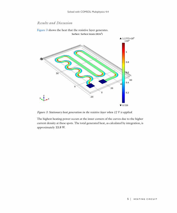
Solved with COMSOL Multiphysics 4.4
Results and Discussion
Figure 3 shows the heat that the resistive layer generates.
Figure 3: Stationary heat generation in the resistive layer when 12 V is applied.
The highest heating power occurs at the inner corners of the curves due to the higher current density at these spots. The total generated heat, as calculated by integration, is approximately 13.8 W.
5 | H E A T I N G C I R C U I T
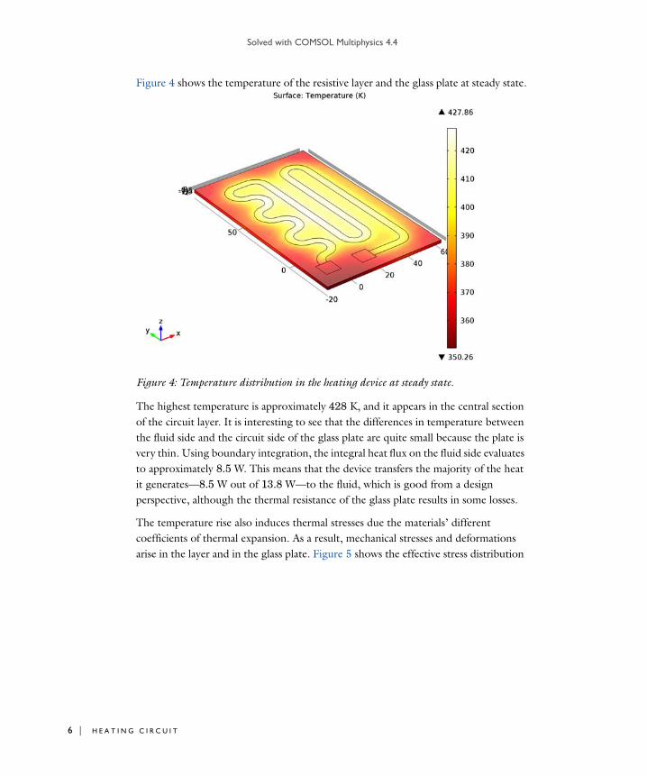
Solved with COMSOL Multiphysics 4.4
6 | H E A
Figure 4 shows the temperature of the resistive layer and the glass plate at steady state.
Figure 4: Temperature distribution in the heating device at steady state.
The highest temperature is approximately 428 K, and it appears in the central section of the circuit layer. It is interesting to see that the differences in temperature between the fluid side and the circuit side of the glass plate are quite small because the plate is very thin. Using boundary integration, the integral heat flux on the fluid side evaluates to approximately 8.5 W. This means that the device transfers the majority of the heat it generates—8.5 W out of 13.8 W—to the fluid, which is good from a design perspective, although the thermal resistance of the glass plate results in some losses.
The temperature rise also induces thermal stresses due the materials’ different coefficients of thermal expansion. As a result, mechanical stresses and deformations arise in the layer and in the glass plate. Figure 5 shows the effective stress distribution
T I N G C I R C U I T

Solved with COMSOL Multiphysics 4.4
in the device and the resulting deformations. During operation, the glass plate bends towards the air side.
Figure 5: The thermally induced von Mises effective stress plotted with the deformation.
The highest effective stress, approximately 13 MPa, occurs at the inner corners of the curves of the Nichrome circuit. The yield stress for high quality glass is roughly 250 MPa, and for Nichrome it is 360 MPa. This means that the individual objects remain structurally intact for the simulated heating power loads.
You must also consider stresses in the interface between the resistive layer and the glass plate. Assume that the yield stress of the surface adhesion in the interface is in the region of 50 MPa—a value significantly lower than the yield stresses of the other materials in the device. If the effective stress increases above this value, the resistive layer will locally detach from the glass. Once it has detached, heat transfer is locally impeded, which can lead to overheating of the resistive layer and eventually cause the device to fail.
Figure 6 displays the effective forces acting on the adhesive layer during heater operation. As the figure shows, the device experiences a maximum interfacial stress that is an order of magnitude smaller than the yield stress. This means that the device will be OK in terms of adhesive stress.
7 | H E A T I N G C I R C U I T

Solved with COMSOL Multiphysics 4.4
8 | H E A
Figure 6: The effective forces in the interface between the resistive layer and the glass plate.
Finally study the device’s deflections, depicted in Figure 7.
Figure 7: Total displacement on the fluid side of the glass plate.
T I N G C I R C U I T

Solved with COMSOL Multiphysics 4.4
The maximum displacement, located at the center of the plate, is approximately 50 µm. For high-precision applications, such as semiconductor processing, this might be a significant value that limits the device’s operating temperature.
Model Library path: Structural_Mechanics_Module/Thermal-Structure_Interaction/heating_circuit
Modeling Instructions
From the File menu, choose New.
N E W
1 In the New window, click the Model Wizard button.
M O D E L W I Z A R D
1 In the Model Wizard window, click the 3D button.
2 In the Select Physics tree, select Structural Mechanics>Thermal Stress.
3 Click the Add button.
4 In the Select Physics tree, select AC/DC>Electric Currents, Shell (ecs).
5 Click the Add button.
6 In the Select Physics tree, select Structural Mechanics>Shell (shell).
7 Click the Add button.
8 Click the Study button.
9 In the Select Study tree, select Preset Studies for Selected Physics>Stationary.
10 Click the Done button.
G E O M E T R Y 1
The Thermal Stress physics interface includes Solid Mechanics and Heat Transfer in Solids. In the volume, these two interfaces solve for temperature and displacement, respectively. In the shell representing the circuit, only the temperature is solved, by Heat Transfer in Solids. The Electric Currents, Shell and Shell physics interfaces only apply on the circuit shell. They solve for electric potential and for the displacement, respectively.
9 | H E A T I N G C I R C U I T
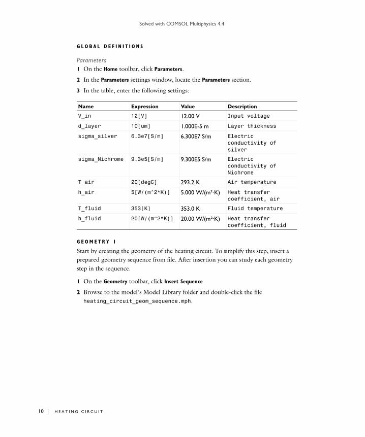
Solved with COMSOL Multiphysics 4.4
10 | H E
G L O B A L D E F I N I T I O N S
Parameters1 On the Home toolbar, click Parameters.
2 In the Parameters settings window, locate the Parameters section.
3 In the table, enter the following settings:
G E O M E T R Y 1
Start by creating the geometry of the heating circuit. To simplify this step, insert a prepared geometry sequence from file. After insertion you can study each geometry step in the sequence.
1 On the Geometry toolbar, click Insert Sequence
2 Browse to the model’s Model Library folder and double-click the file heating_circuit_geom_sequence.mph.
Name Expression Value Description
V_in 12[V] 12.00 V Input voltage
d_layer 10[um] 1.000E-5 m Layer thickness
sigma_silver 6.3e7[S/m] 6.300E7 S/m Electric conductivity of silver
sigma_Nichrome 9.3e5[S/m] 9.300E5 S/m Electric conductivity of Nichrome
T_air 20[degC] 293.2 K Air temperature
h_air 5[W/(m^2*K)] 5.000 W/(m²·K) Heat transfer coefficient, air
T_fluid 353[K] 353.0 K Fluid temperature
h_fluid 20[W/(m^2*K)] 20.00 W/(m²·K) Heat transfer coefficient, fluid
A T I N G C I R C U I T

Solved with COMSOL Multiphysics 4.4
Work Plane 11 In the Model Builder window, under Component 1>Geometry 1 click Work Plane 1 and
then click Build All Objects.
The model geometry is now complete.
D E F I N I T I O N S
Add a selection that you can use later when applying boundary conditions and shell physics settings.
Explicit 11 On the Definitions toolbar, click Explicit.
2 In the Explicit settings window, locate the Input Entities section.
3 From the Geometric entity level list, choose Boundary.
4 Select Boundaries 6–8 only.
5 Right-click Component 1>Definitions>Explicit 1 and choose Rename.
6 Go to the Rename Explicit dialog box and type Circuit in the New name edit field.
7 Click OK.
11 | H E A T I N G C I R C U I T

Solved with COMSOL Multiphysics 4.4
12 | H E
Before creating the materials for use in this model, it is a good idea to specify which boundaries are to be modeled as conducting shells. Using this information, COMSOL Multiphysics can detect which material properties are needed.
H E A T TR A N S F E R I N S O L I D S
Highly Conductive Layer 11 In the Model Builder window, under Component 1 click Heat Transfer in Solids (ht).
2 On the Physics toolbar, click Boundaries and choose Highly Conductive Layer.
3 In the Highly Conductive Layer settings window, locate the Boundary Selection section.
4 From the Selection list, choose Circuit.
5 Locate the Thermodynamics section. In the ds edit field, type d_layer.
E L E C T R I C C U R R E N T S , S H E L L
1 In the Model Builder window, under Component 1 click Electric Currents, Shell (ecs).
2 In the Electric Currents, Shell settings window, locate the Boundary Selection section.
3 From the Selection list, choose Circuit.
4 Locate the Shell Thickness section. In the ds edit field, type d_layer.
S H E L L
1 In the Model Builder window, under Component 1 click Shell (shell).
2 In the Shell settings window, locate the Boundary Selection section.
3 From the Selection list, choose Circuit.
4 Locate the Thickness section. In the d edit field, type d_layer.
5 Click to expand the Dependent Variables section. In the Displacement field edit field, type u.
Linear Elastic Material 1In the Model Builder window, expand the Shell (shell) node.
Thermal Expansion 11 Right-click Linear Elastic Material 1 and choose Thermal Expansion.
2 In the Thermal Expansion settings window, locate the Model Inputs section.
3 From the T list, choose Temperature (ht).
M A T E R I A L S
On the Home toolbar, click Add Material.
A T I N G C I R C U I T

Solved with COMSOL Multiphysics 4.4
A D D M A T E R I A L
1 Go to the Add Material window.
2 In the tree, select Built-In>Silica glass.
3 In the Add Material window, click Add to Component.
M A T E R I A L S
Now set up the materials.
Material 21 In the Model Builder window, right-click Materials and choose New Material.
2 In the Material settings window, locate the Geometric Entity Selection section.
3 From the Geometric entity level list, choose Boundary.
4 From the Selection list, choose Circuit.
5 Locate the Material Contents section. In the table, enter the following settings:
6 Right-click Component 1>Materials>Material 2 and choose Rename.
7 Go to the Rename Material dialog box and type Silver in the New name edit field.
8 Click OK.
Material 31 Right-click Materials and choose New Material.
2 In the Material settings window, locate the Geometric Entity Selection section.
3 From the Geometric entity level list, choose Boundary.
4 Select Boundary 7 only.
Property Name Value Unit Property group
Thermal conductivity k 420 W/(m·K) Basic
Density rho 10500 kg/m³ Basic
Heat capacity at constant pressure
Cp 230 J/(kg·K) Basic
Relative permittivity epsilonr 1 1 Basic
Electrical conductivity sigma sigma_silver S/m Basic
Young's modulus E 83e9 Pa Basic
Poisson's ratio nu 0.37 1 Basic
Coefficient of thermal expansion
alpha 18.9e-6 1/K Basic
13 | H E A T I N G C I R C U I T

Solved with COMSOL Multiphysics 4.4
14 | H E
5 Locate the Material Contents section. In the table, enter the following settings:
6 Right-click Component 1>Materials>Material 3 and choose Rename.
7 Go to the Rename Material dialog box and type Nichrome in the New name edit field.
8 Click OK.
With the materials defined, set up the remaining physics of the model. In the next section, the resistive loss within the circuit is defined as a heat source. The resistive loss is calculated automatically within the Electric Currents, Shell physics. Add the coupling feature Boundary Electromagnetic Heat Source to take the resistive loss into account.
M U L T I P H Y S I C S
1 In the Model Builder window, under Component 1 right-click Multiphysics and choose Boundary Electromagnetic Heat Source.
2 In the Boundary Electromagnetic Heat Source settings window, locate the Boundary
Selection section.
3 From the Selection list, choose Circuit.
H E A T TR A N S F E R I N S O L I D S
Convective Heat Flux 11 In the Model Builder window, under Component 1 click Heat Transfer in Solids (ht).
2 On the Physics toolbar, click Boundaries and choose Convective Heat Flux.
3 Select Boundaries 4 and 6–8 only.
4 In the Convective Heat Flux settings window, locate the Heat Flux section.
Property Name Value Unit Property group
Thermal conductivity k 15 W/(m·K) Basic
Density rho 9000 kg/m³ Basic
Heat capacity at constant pressure
Cp 20 J/(kg·K) Basic
Relative permittivity epsilonr 1 1 Basic
Electrical conductivity sigma sigma_Nichrome S/m Basic
Young's modulus E 213e9 Pa Basic
Poisson's ratio nu 0.33 1 Basic
Coefficient of thermal expansion
alpha 10e-6 1/K Basic
A T I N G C I R C U I T

Solved with COMSOL Multiphysics 4.4
5 In the h edit field, type h_air.
6 In the Text edit field, type T_air.
Convective Heat Flux 21 On the Physics toolbar, click Boundaries and choose Convective Heat Flux.
2 Select Boundary 3 only.
3 In the Convective Heat Flux settings window, locate the Heat Flux section.
4 In the h edit field, type h_fluid.
5 In the Text edit field, type T_fluid.
Next, add constraints to restrain the glass plate movements.
S O L I D M E C H A N I C S
Fixed Constraint 11 In the Model Builder window, under the Component 1 click Solid Mechanics (solid).
2 On the Physics toolbar, click Points and choose Fixed Constraint.
3 Select Point 1 only.
Prescribed Displacement 11 On the Physics toolbar, click Points and choose Prescribed Displacement.
2 Select Point 63 only.
3 In the Prescribed Displacement settings window, locate the Prescribed Displacement section.
4 Select the Prescribed in y direction check box.
5 Select the Prescribed in z direction check box.
Prescribed Displacement 21 On the Physics toolbar, click Points and choose Prescribed Displacement.
2 Select Point 3 only.
3 In the Prescribed Displacement settings window, locate the Prescribed Displacement section.
4 Select the Prescribed in z direction check box.
Finally, add a voltage and ground.
15 | H E A T I N G C I R C U I T

Solved with COMSOL Multiphysics 4.4
16 | H E
E L E C T R I C C U R R E N T S , S H E L L
Electric Potential 11 In the Model Builder window, under Component 1 click Electric Currents, Shell (ecs).
2 On the Physics toolbar, click Edges and choose Electric Potential.
3 Select Edge 10 only.
4 In the Electric Potential settings window, locate the Electric Potential section.
5 In the V0 edit field, type V_in.
Ground 11 On the Physics toolbar, click Edges and choose Ground.
2 Select Edge 43 only.
M E S H 1
Use a relatively coarse mesh to reduce the model size.
Free Triangular 11 In the Model Builder window, under Component 1 right-click Mesh 1 and choose Free
Triangular.
2 Select Boundaries 4 and 6–8 only.
Size 11 Right-click Component 1>Mesh 1>Free Triangular 1 and choose Size.
2 In the Size settings window, locate the Geometric Entity Selection section.
3 From the Selection list, choose Circuit.
4 Locate the Element Size section. Click the Custom button.
5 Locate the Element Size Parameters section. Select the Maximum element size check box.
6 In the associated edit field, type 4.
Swept 1In the Model Builder window, right-click Mesh 1 and choose Swept.
Distribution 11 In the Model Builder window, under Component 1>Mesh 1 right-click Swept 1 and
choose Distribution.
2 In the Distribution settings window, locate the Distribution section.
3 In the Number of elements edit field, type 2.
A T I N G C I R C U I T

Solved with COMSOL Multiphysics 4.4
4 Click the Build All button.
S T U D Y 1
On the Home toolbar, click Compute.
R E S U L T S
Stress (solid)The default plots show the von Mises stress including the deformation (Figure 5) and the temperature (Figure 4) on the surface of the full 3D geometry, the electric potential on the circuit layer, and the von Mises stress on the top and bottom of the circuit layer.
To generate Figure 3 follow the steps below.
3D Plot Group 71 On the Home toolbar, click Add Plot Group and choose 3D Plot Group.
2 In the Model Builder window, under Results right-click 3D Plot Group 7 and choose Surface.
3 In the Surface settings window, locate the Expression section.
4 Click Replace Expression button in the upper-right corner of the Expression section. From the menu, choose Electric Currents, Shell>Heating and losses>Surface losses
(ecs.Qsh). Double-click or press Enter.
5 On the 3D Plot Group toolbar, click Plot.
6 Click the Scene Light button on the Graphics toolbar.
7 Click the Zoom Extents button on the Graphics toolbar.
8 In the Model Builder window, right-click 3D Plot Group 7 and choose Rename.
9 Go to the Rename 3D Plot Group dialog box and type Surface Losses in the New
name edit field.
10 Click OK.
The following steps generate a plot of the norm of the surface traction vector in the surface plane (see Figure 6):
Data Sets1 In the Model Builder window, under Results>Data Sets right-click Solution 1 and
choose Duplicate.
2 Right-click Results>Data Sets>Solution 2 and choose Add Selection.
3 In the Selection settings window, locate the Geometric Entity Selection section.
17 | H E A T I N G C I R C U I T

Solved with COMSOL Multiphysics 4.4
18 | H E
4 From the Geometric entity level list, choose Boundary.
5 From the Selection list, choose Circuit.
3D Plot Group 81 On the Home toolbar, click Add Plot Group and choose 3D Plot Group.
2 In the 3D Plot Group settings window, locate the Data section.
3 From the Data set list, choose Solution 2.
4 Right-click Results>3D Plot Group 8 and choose Surface.
5 In the Surface settings window, locate the Expression section.
6 In the Expression edit field, type sqrt(solid.Tax^2+solid.Tay^2).
7 From the Unit list, choose MPa.
8 On the 3D Plot Group toolbar, click Plot.
9 In the Model Builder window, right-click 3D Plot Group 8 and choose Rename.
10 Go to the Rename 3D Plot Group dialog box and type Interface Stress in the New
name edit field.
11 Click OK.
Finally, to obtain Figure 7, proceed as follows:
Data Sets1 On the Results toolbar, click More Data Sets and choose Surface.
2 Select Boundary 3 only.
2D Plot Group 91 On the Home toolbar, click Add Plot Group and choose 2D Plot Group.
2 In the Model Builder window, under Results right-click 2D Plot Group 9 and choose Surface.
3 In the Surface settings window, locate the Expression section.
4 Click Replace Expression button in the upper-right corner of the Expression section. From the menu, choose Solid Mechanics>Displacement>Total displacement
(solid.disp). Double-click or press Enter.
5 From the Unit list, choose um.
6 On the 2D Plot Group toolbar, click Plot.
7 In the Model Builder window, right-click 2D Plot Group 9 and choose Rename.
8 Go to the Rename 2D Plot Group dialog box and type Displacement, bottom boundary in the New name edit field.
A T I N G C I R C U I T

Solved with COMSOL Multiphysics 4.4
9 Click OK.
Derived ValuesTo calculate the values for the total generated heat and the integrated heat flux on the fluid side, perform a boundary integration:
1 On the Results toolbar, click More Derived Values and choose Integration>Surface
Integration.
2 Select Boundary 3 only.
3 In the Surface Integration settings window, locate the Expression section.
4 Click Replace Expression button in the upper-right corner of the Expression section. From the menu, choose Heat Transfer in Solids>Boundary fluxes>Boundary convective
heat flux (ht.chflux). Double-click or press Enter.
5 Click the Evaluate button.
TA B L E
The result should be close to 8.5 W.
R E S U L T S
Derived Values1 On the Results toolbar, click More Derived Values and choose Integration>Surface
Integration.
2 In the Surface Integration settings window, locate the Selection section.
3 From the Selection list, choose Circuit.
4 Click Replace Expression button in the upper-right corner of the Expression section. From the menu, choose Electric Currents, Shell>Heating and losses>Surface losses
(ecs.Qsh). Double-click or press Enter.
TA B L E
The result should be close to 13.8 W.
19 | H E A T I N G C I R C U I T

Solved with COMSOL Multiphysics 4.4
20 | H E
A T I N G C I R C U I T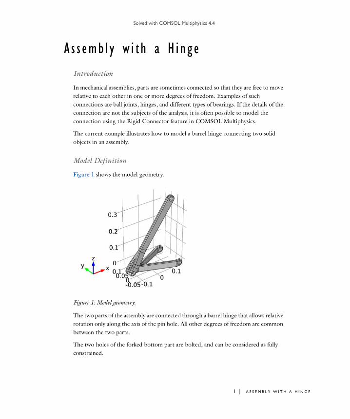
Solved with COMSOL Multiphysics 4.4
A s s emb l y w i t h a H i n g e
Introduction
In mechanical assemblies, parts are sometimes connected so that they are free to move relative to each other in one or more degrees of freedom. Examples of such connections are ball joints, hinges, and different types of bearings. If the details of the connection are not the subjects of the analysis, it is often possible to model the connection using the Rigid Connector feature in COMSOL Multiphysics.
The current example illustrates how to model a barrel hinge connecting two solid objects in an assembly.
Model Definition
Figure 1 shows the model geometry.
Figure 1: Model geometry.
The two parts of the assembly are connected through a barrel hinge that allows relative rotation only along the axis of the pin hole. All other degrees of freedom are common between the two parts.
The two holes of the forked bottom part are bolted, and can be considered as fully constrained.
1 | A S S E M B L Y W I T H A H I N G E

Solved with COMSOL Multiphysics 4.4
2 | A S S
The pin hole of the top part is constrained in the x direction so that it can slide in the y-z plane.
A force of 1 kN is applied in z direction at a 10 cm distance in the negative y direction from the center of the upper pin hole. The offset of the load will thus introduce both tension and bending of the member.
Results and Discussion
The default plot shown in Figure 2 shows the von Mises stress in the model. You can see the bending of the top part due to the offset of the load. You can also see the stress that is transmitted around the hinge.
In Figure 3 the color gradient in the x displacement indicates that the lower part of the assembly undergoes bending around y axis. With a constraint rotation in y direction bending from one part would progress to the second part. The upper part however shows a fairly constant displacement through the height, which indicates that is not being bent in y direction and thus it has a free rotation in y direction in the connection point.
E M B L Y W I T H A H I N G E
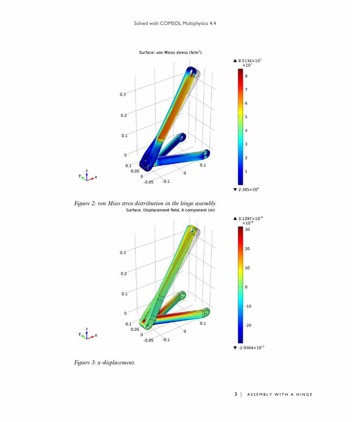
Solved with COMSOL Multiphysics 4.4
Figure 2: von Mises stress distribution in the hinge assembly.
Figure 3: x-displacement.
3 | A S S E M B L Y W I T H A H I N G E

Solved with COMSOL Multiphysics 4.4
4 | A S S
Notes About the COMSOL Implementation
The approach when modeling mechanisms is to attach rigid connectors to both parts, make sure that they have a common center of rotation, and then couple relevant degrees of freedom between them in order to obtain the desired function.
When you model a hinge, all translations and two rotations should be equal in the two parts. As in this case the displacement and the rotation in the hinge remain small, the procedure simply consists of linking the displacement in all directions as well as the rotation around the x and z directions. You connect the displacements of the rigid connectors directly using the prescribed displacement setting available in the rigid connector feature. In order to constrain the rotation directions independently, you need however to add two global constraints, one for each rotational degree of freedom. The rigid connector uses a quaternion representation of the rotation; see the section Theory for the Rigid Connector in the Structural Mechanics User’s Guide. In this specific example both the b and the d rotation variables are coupled between the two rigid connectors, because they directly correspond to the intended rotation angles for small rotations.
Another rigid connector is also used for applying the force to the upper pin hole.
Model Library path: Structural_Mechanics_Module/Connectors_and_Mechanisms/hinge_assembly
Modeling Instructions
From the File menu, choose New.
N E W
1 In the New window, click the Model Wizard button.
M O D E L W I Z A R D
1 In the Model Wizard window, click the 3D button.
2 In the Select physics tree, select Structural Mechanics>Solid Mechanics (solid).
3 Click the Add button.
4 Click the Study button.
5 In the tree, select Preset Studies>Stationary.
E M B L Y W I T H A H I N G E

Solved with COMSOL Multiphysics 4.4
6 Click the Done button.
G L O B A L D E F I N I T I O N S
Parameters1 On the Home toolbar, click Parameters.
2 In the Parameters settings window, locate the Parameters section.
3 In the table, enter the following settings:
G E O M E T R Y 1
Import 11 On the Home toolbar, click Import.
2 In the Import settings window, locate the Import section.
3 Click the Browse button.
4 Browse to the model’s Model Library folder and double-click the file hinge_assembly.mphbin.
5 Click the Import button.
Form Union1 In the Model Builder window, under Component 1>Geometry 1 click Form Union.
2 In the Form Union/Assembly settings window, locate the Form Union/Assembly section.
3 From the Action list, choose Form an assembly.
4 Clear the Create pairs check box.
5 Click the Build Selected button.
M A T E R I A L S
On the Home toolbar, click Add Material.
A D D M A T E R I A L
1 Go to the Add Material window.
2 In the tree, select Built-In>Structural steel.
3 In the Add material window, click Add to Component.
4 On the Home toolbar, click Add Material to close the add material window.
Name Expression Value Description
F 1e3[N] 1000 N Applied load
5 | A S S E M B L Y W I T H A H I N G E

Solved with COMSOL Multiphysics 4.4
6 | A S S
S O L I D M E C H A N I C S
Fixed Constraint 11 On the Physics toolbar, click Boundaries and choose Fixed Constraint.
2 Select Boundaries 133–136 only.
Rigid Connector 11 On the Physics toolbar, click Boundaries and choose Rigid Connector.
2 Select Boundaries 67 and 68 only.
3 In the Rigid Connector settings window, locate the Prescribed Displacement at Center
of Rotation section.
4 Select the Prescribed in x direction check box.
Applied Force 11 Right-click Component 1>Solid Mechanics>Rigid Connector 1 and choose Applied
Force.
2 In the Applied Force settings window, locate the Location section.
3 From the list, choose User defined (absolute).
4 Specify the Xp vector as
The center of rotation for a rigid connector is available in the variables xcX_<tag>, xcY_<tag>, and xcZ_<tag>. The default position is the center of gravity of the attached boundaries, which in this case will be the center of the hole.
5 Locate the Applied Force section. Specify the F vector as
Rigid Connector 21 On the Physics toolbar, click Boundaries and choose Rigid Connector.
2 Select Boundaries 75 and 76 only.
solid.xcX_rig1 X
solid.xcY_rig1-0.1 Y
solid.xcZ_rig1 Z
0 x
0 y
F z
E M B L Y W I T H A H I N G E

Solved with COMSOL Multiphysics 4.4
Rigid Connector 31 On the Physics toolbar, click Boundaries and choose Rigid Connector.
2 Select Boundaries 16–19 only.
Set the translations of this rigid connector equal to the translations of the second rigid connector.
3 In the Rigid Connector settings window, locate the Prescribed Displacement at Center
of Rotation section.
4 Select the Prescribed in x direction check box.
5 In the u0x edit field, type solid.rig2.u.
6 Select the Prescribed in y direction check box.
7 In the u0y edit field, type solid.rig2.v.
8 Select the Prescribed in z direction check box.
9 In the u0z edit field, type solid.w_rig2.
Connect the rotations around the x and z directions, using the quaternion degrees of freedom 'b' and 'd'.
1 In the Model Builder window’s toolbar, click the Show button and select Advanced
Physics Options in the menu.
Global Constraint 11 On the Physics toolbar, click Global and choose Global Constraint.
2 In the Global Constraint settings window, locate the Global Constraint section.
3 In the Constraint expression edit field, type comp1.solid.rig2.b-comp1.solid.rig3.b.
Global Constraint 21 On the Physics toolbar, click Global and choose Global Constraint.
2 In the Global Constraint settings window, locate the Global Constraint section.
3 In the Constraint expression edit field, type comp1.solid.rig2.d-comp1.solid.rig3.d.
M E S H 1
Free Tetrahedral 1In the Model Builder window, under Component 1 right-click Mesh 1 and choose Free Tetrahedral.
7 | A S S E M B L Y W I T H A H I N G E

Solved with COMSOL Multiphysics 4.4
8 | A S S
Size 11 In the Model Builder window, under Component 1>Mesh 1 right-click Free Tetrahedral
1 and choose Size.
2 In the Size settings window, locate the Geometric Entity Selection section.
3 From the Geometric entity level list, choose Boundary.
4 Select Boundaries 41, 42, and 53 only.
5 Locate the Element Size section. Click the Custom button.
6 Locate the Element Size Parameters section. Select the Maximum element size check box.
7 In the associated edit field, type 0.002.
Size1 In the Model Builder window, under Component 1>Mesh 1 click Size.
2 In the Size settings window, locate the Element Size section.
3 From the Predefined list, choose Fine.
4 Click the Build All button.
S T U D Y 1
On the Home toolbar, click Compute.
R E S U L T S
Stress (solid)The default plot shows the von Mises stress distribution on the surface of the assembly. Compare with Figure 2.
Finally, reproduce the x-displacement plot shown in Figure 3 with the following steps:
Stress (solid) 11 In the Model Builder window, under Results right-click Stress (solid) and choose
Duplicate.
2 In the Model Builder window, expand the Stress (solid) 1 node, then click Surface 1.
3 In the Surface settings window, click Replace Expression in the upper-right corner of the Expression section. From the menu, choose Solid
Mechanics>Displacement>Displacement field (Material)>Displacement field, X
component (u).
4 On the Stress (solid) 1 toolbar, click Plot.
E M B L Y W I T H A H I N G E

Solved with COMSOL Multiphysics 4.4
5 In the Model Builder window, right-click Stress (solid) 1 and choose Rename.
6 Go to the Rename 3D Plot Group dialog box and type x-Displacement in the New
name edit field.
7 Click OK.
9 | A S S E M B L Y W I T H A H I N G E

Solved with COMSOL Multiphysics 4.4
10 | A S
S E M B L Y W I T H A H I N G E
Solved with COMSOL Multiphysics 4.4
V i b r a t i o n s o f an Impe l l e r
Introduction
This tutorial model demonstrates the use of dynamic cyclic symmetry with postprocessing on the full geometry. A 3D impeller with eight identical blades can be divided into eight sectors of symmetry. The model computes the fundamental frequencies for the full impeller geometry and compares them to the values computed for a single sector with the cyclic symmetry boundary conditions applied on two sector boundaries. It also demonstrates how to set up a frequency response analysis for one sector of symmetry, and how to postprocess the results into the full geometry by using the sector data sets. The results for one sector are in very good agreement with the computations on the full geometry, while both the computational time and memory requirements are significantly reduced.
Model Definition
Figure 1 shows the impeller geometry. The problem is solved using the cartesian coordinate system in 3D.
Figure 1: Impeller geometry.
1 | V I B R A T I O N S O F A N I M P E L L E R

Solved with COMSOL Multiphysics 4.4
2 | V I B R
The geometry can be divided into eight identical parts, each represented by a sector with an angle 4 about the z-axis; see Figure 2.
Figure 2: Sector of periodicity.
The impeller is made of aluminum, and is supposed to be mounted on a shaft. The mounting boundary is modeled via a fixed constraint, and all possible effects of the shaft rotation are neglected.
The analysis is based on the Floquet theory which can be applied to the problem of small-amplitude vibrations of spatially periodic structures, Ref. 1. This includes the case of cyclic symmetry studied in this model.
For an eigenfrequency study, one can show that all the eigenmodes of the full problem can be found by performing the analysis on one sector of symmetry only and imposing the cyclic symmetry of the eigenmodes with an angle of periodicity , where the cyclic symmetry mode number m can vary from 0 to N, with N being the total number of sectors so that 2N.
Results and Discussion
In the first part of the analysis, you perform an eigenfrequency analysis of a single sector of periodicity, and then of the full geometry. A sweep over all required values of the cyclic symmetry parameter recovers all the eigenfrequencies of the full model with
m=
A T I O N S O F A N I M P E L L E R

Solved with COMSOL Multiphysics 4.4
decent accuracy. See the Modeling Instructions section for in-detail comparison of the results and discussion of the performance gains.
In the second part, you perform a frequency-response analysis. Again, first of the sector of periodicity, and then of the full impeller geometry. The excitation is a pressure load applied to all free boundaries of the impeller. You enter it as a normal component of the boundary load using the expression
using the magnitude of p0 = 104 Pa and cyclic symmetry parameter m = 3. The excitation frequency is 200 Hz. Figure 3 and Figure 4 show very good agreement between the results computed on the full and reduced geometry.
Fn p0 jm Y X atan– exp–=
3 | V I B R A T I O N S O F A N I M P E L L E R

Solved with COMSOL Multiphysics 4.4
4 | V I B R
Figure 3: Frequency response computed on the sector of periodicity only, and then visualized over the full geometry.
Figure 4: Frequency response computed for the full geometry.
A T I O N S O F A N I M P E L L E R
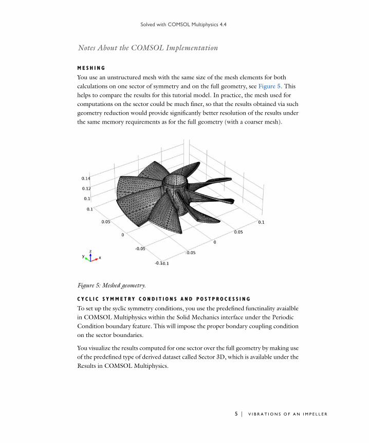
Solved with COMSOL Multiphysics 4.4
Notes About the COMSOL Implementation
M E S H I N G
You use an unstructured mesh with the same size of the mesh elements for both calculations on one sector of symmetry and on the full geometry, see Figure 5. This helps to compare the results for this tutorial model. In practice, the mesh used for computations on the sector could be much finer, so that the results obtained via such geometry reduction would provide significantly better resolution of the results under the same memory requirements as for the full geometry (with a coarser mesh).
Figure 5: Meshed geometry.
C Y C L I C S Y M M E T RY C O N D I T I O N S A N D PO S T P R O C E S S I N G
To set up the syclic symmetry conditions, you use the predefined functinality avaialble in COMSOL Multiphysics within the Solid Mechanics interface under the Periodic Condition boundary feature. This will impose the proper bondary coupling condition on the sector boundaries.
You visualize the results computed for one sector over the full geometry by making use of the predefined type of derived dataset called Sector 3D, which is available under the Results in COMSOL Multiphysics.
5 | V I B R A T I O N S O F A N I M P E L L E R

Solved with COMSOL Multiphysics 4.4
6 | V I B R
Reference
1. B. Lalanne and M. Touratier, “Aeroelastic Vibrations and Stability in Cyclic Symmetric Domains,” Int. J. Rotating Machinery, vol. 6, no. 6, pp 445–452, 2000.
Model Library path: Structural_Mechanics_Module/Dynamics_and_Vibration/impeller
Modeling Instructions
From the File menu, choose New.
N E W
1 In the New window, click the Model Wizard button.
M O D E L W I Z A R D
1 In the Model Wizard window, click the 3D button.
2 In the Select physics tree, select Structural Mechanics>Solid Mechanics (solid).
3 Click the Add button.
4 Click the Study button.
5 In the tree, select Preset Studies>Eigenfrequency.
6 Click the Done button.
G E O M E T R Y 1
Import the pre-built geometry for the impeller from a file.
Import 11 On the Home toolbar, click Import.
2 In the Import settings window, locate the Import section.
3 Click the Browse button.
4 Browse to the model’s Model Library folder and double-click the file impeller.mphbin.
5 Click the Import button.
6 Click the Go to Default 3D View button on the Graphics toolbar.
7 On the Home toolbar, click Build All.
A T I O N S O F A N I M P E L L E R

Solved with COMSOL Multiphysics 4.4
8 Click the Go to Default 3D View button on the Graphics toolbar.
9 Click the Go to XY View button on the Graphics toolbar.
The complete geometry should look similar to that shown in Figure 1 and Figure 2.
G L O B A L D E F I N I T I O N S
Parameters1 On the Home toolbar, click Parameters.
2 In the Parameters settings window, locate the Parameters section.
3 In the table, enter the following settings:
C O M P O N E N T 1
Add a second Solid Mechanics interface to use for the computations on the reduced geometry only.
1 On the Home toolbar, click Add Physics.
A D D P H Y S I C S
1 Go to the Add Physics window.
2 In the Add Physics tree, select Structural Mechanics>Solid Mechanics (solid).
3 In the Add Physics window, click Add to Component.
4 On the Home toolbar, click Add Physics.
S O L I D M E C H A N I C S 2
1 In the Model Builder window, under Component 1 click Solid Mechanics 2.
2 Select Domain 8 only.
M A T E R I A L S
On the Home toolbar, click Add Material.
A D D M A T E R I A L
1 Go to the Add Material window.
Name Expression Value Description
N 8 8.000 Number of sectors
theta 2*pi/N 0.7854 Unit sector angle
m 3 3.000 Azimuthal mode number
p0 1e4[Pa] 1.000E4 Pa Load magnitude
7 | V I B R A T I O N S O F A N I M P E L L E R

Solved with COMSOL Multiphysics 4.4
8 | V I B R
2 In the tree, select Built-In>Aluminum.
3 In the Add material window, click Add to Component.
4 On the Home toolbar, click Add Material.
S O L I D M E C H A N I C S
Fixed Constraint 11 On the Physics toolbar, click Boundaries and choose Fixed Constraint.
2 Select Boundaries 54, 55, 67, 68, 85, 87, 109, and 113 only.
S O L I D M E C H A N I C S 2
1 On the Physics toolbar, click Boundaries and choose Fixed Constraint.
2 Select Boundary 113 only.
For a reduced geometry, you set up the cyclic symmetry condition on the sector boundaries.
Periodic Condition 11 On the Physics toolbar, click Boundaries and choose Periodic Condition.
2 Select Boundaries 112 and 134 only.
3 In the Periodic Condition settings window, locate the Periodicity Settings section.
4 From the Type of periodicity list, choose Cyclic symmetry.
5 In the m edit field, type m.
Destination Selection 11 Right-click Component 1>Solid Mechanics 2>Periodic Condition 1 and choose
Destination Selection.
2 In the Destination Selection settings window, locate the Boundary Selection section.
3 Click Clear Selection.
4 Select Boundary 112 only.
Follow these steps to create a free unstructured mesh that will be identical in all eight sectors.
M E S H 1
1 In the Model Builder window, under Component 1 click Mesh 1.
2 In the Mesh settings window, locate the Mesh Settings section.
3 From the Element size list, choose Fine.
A T I O N S O F A N I M P E L L E R

Solved with COMSOL Multiphysics 4.4
Free Triangular 11 Right-click Component 1>Mesh I and choose More Operations>Free Triangular.
2 Select Boundary 134 only.
Copy Face 11 In the Model Builder window, right-click Mesh 1 and choose More Operations>Copy
Face.
2 Select Boundary 134 only.
3 In the Copy Face settings window, locate the Destination Boundaries section.
4 Select Boundary 112 only.
Free Tetrahedral 11 Right-click Mesh 1 and choose Free Tetrahedral.
2 In the Free Tetrahedral settings window, locate the Domain Selection section.
3 From the Geometric entity level list, choose Domain.
4 Select Domain 8 only.
5 Click the Build Selected button.
Copy Domain 11 Right-click Mesh 1 and choose More Operations>Copy Domain.
2 Select Domain 8 only.
3 In the Copy Domain settings window, locate the Destination Domains section.
4 Select Domains 1–5 only.
5 Click the Build Selected button.
Copy Domain 21 Right-click Mesh 1 and choose More Operations>Copy Domain.
2 Select Domain 1 only.
3 In the Copy Domain settings window, locate the Destination Domains section.
4 Select Domains 6 and 7 only.
5 Right-click Mesh 1 and choose Build All.
6 Click the Go to Default 3D View button on the Graphics toolbar.
The resulting mesh should look similar to that shown in Figure 5.
9 | V I B R A T I O N S O F A N I M P E L L E R

Solved with COMSOL Multiphysics 4.4
10 | V I B
S T U D Y 1
Step 1: Eigenfrequency1 In the Model Builder window, expand the Study 1 node, then click Step 1:
Eigenfrequency.
2 In the Eigenfrequency settings window, locate the Physics and Variables Selection section.
3 In the table, enter the following settings:
4 Locate the Study Settings section. In the Desired number of eigenfrequencies edit field, type 32.
Solver 11 On the Study toolbar, click Show Default Solver.
2 In the Model Builder window, expand the Study 1>Solver Configurations>Solver
1>Dependent Variables 1 node, then click Displacement field (Material) (comp1.u2).
3 In the Field settings window, locate the General section.
4 Clear the Store in output check box.
5 On the Home toolbar, click Compute.
R O O T
On the Home toolbar, click Add Study.
A D D S T U D Y
1 Go to the Add Study window.
2 Find the Studies subsection. In the tree, select Preset Studies>Eigenfrequency.
3 Find the Physics in study subsection. In the table, enter the following settings:
4 In the Add study window, click Add Study.
5 On the Home toolbar, click Add Study.
Physics Solve for Discretization
Solid Mechanics 2 × physics
Physics Solve
Solid Mechanics (solid) ×
R A T I O N S O F A N I M P E L L E R

Solved with COMSOL Multiphysics 4.4
S T U D Y 2
Step 1: Eigenfrequency1 In the Model Builder window, under Study 2 click Step 1: Eigenfrequency.
2 In the Eigenfrequency settings window, locate the Study Settings section.
3 In the Desired number of eigenfrequencies edit field, type 4.
To capture all possible eigenfrequencies, set up a sweep over the cyclic symmetry mode number m in the range from 0 to N/2, where N is the total number of sectors.
Parametric Sweep1 On the Study toolbar, click Extension Steps and choose Parametric Sweep.
2 In the Parametric Sweep settings window, locate the Study Settings section.
3 Click Add.
4 In the table, enter the following settings:
5 Click Range.
6 Go to the Range dialog box.
7 In the Start edit field, type 0.
8 In the Stop edit field, type N/2.
9 In the Step edit field, type 1.
10 Click the Add button.
Solver 21 On the Study toolbar, click Show Default Solver.
2 In the Model Builder window, expand the Study 2>Solver Configurations>Solver
2>Dependent Variables 1 node, then click Displacement field (Material) (comp1.u).
3 In the Field settings window, locate the General section.
4 Clear the Store in output check box.
5 On the Home toolbar, click Compute.
Parameter names Parameter value list
m
11 | V I B R A T I O N S O F A N I M P E L L E R

Solved with COMSOL Multiphysics 4.4
12 | V I B
R E S U L T S
Mode Shape (solid2)Note a nearly eight times reduction in the number of degrees of freedom, and thus of the memory required to compute the reduced model. However, the computational time is approximately the same because you need to perform a sweep over all values of the periodicity parameter.
Add a new dataset to visualize over the full geometry the eigenmode shape for the reduced model.
Data Sets1 On the Results toolbar, click More Data Sets and choose Sector 3D.
2 In the Sector 3D settings window, locate the Data section.
3 From the Data set list, choose Solution 3.
4 Locate the Symmetry section. In the Number of sectors edit field, type 8.
5 Click to expand the Advanced section. In the Azimuthal mode number edit field, type 4.
Mode Shape (solid2)1 In the Model Builder window, under Results click Mode Shape (solid2).
2 In the 3D Plot Group settings window, locate the Data section.
3 From the Data set list, choose Sector 3D 1.
4 On the Mode Shape (solid2) toolbar, click Plot.
Derived ValuesCollect all the computed eigenfrequencies into tables.
1 On the Results toolbar, click Global Evaluation.
2 In the Global Evaluation settings window, locate the Expression section.
3 In the Expression edit field, type freq.
4 Right-click Results>Derived Values>Global Evaluation 1 and choose Evaluate>New
Table.
TA B L E
Note that the eigenfrequencies for the full geometry present groups of values very close to each other, eight frequencies in each group. This shows that vibrations of each of the eight blades of the impeller are only weakly coupled to the remaining structure, which happens because the central part has significantly larger effective
R A T I O N S O F A N I M P E L L E R

Solved with COMSOL Multiphysics 4.4
bending stiffness compared to that of each blade. Hence, the eigenfrequencies in each group are close to the natural frequencies of a single blade (if computed assuming a fully fixed footing).
R E S U L T S
Derived Values1 On the Results toolbar, click Global Evaluation.
2 In the Global Evaluation settings window, locate the Data section.
3 From the Data set list, choose Solution 3.
4 From the Table columns list, choose Inner solutions.
5 Locate the Expression section. In the Expression edit field, type freq.
6 Right-click Results>Derived Values>Global Evaluation 2 and choose Evaluate>New
Table.
TA B L E
Compare the values of the egenfrequencies computed by using the periodicity conditions to those found for the full geometry.
Next, add a load representing a periodic pressure perturbation in the stream, and thus on all the external boundaries of the impeller.
S O L I D M E C H A N I C S
Boundary Load 11 On the Physics toolbar, click Boundaries and choose Boundary Load.
2 In the Boundary Load settings window, locate the Boundary Selection section.
3 Select Boundaries 1–3, 5–18, 20, 21, 23–53, 56–66, 69–75, 77–84, 88–107, 110, 111, 114–133, and 135–152 only.
You can do this by selecting all boundaries first, and then removing from the selection all the constraint boundaries and all the internal boundaries of the periodicity sectors.
4 Locate the Coordinate System Selection section. From the Coordinate system list, choose Boundary System 1.
5 Locate the Force section. Specify the FA vector as
0 t1
13 | V I B R A T I O N S O F A N I M P E L L E R

Solved with COMSOL Multiphysics 4.4
14 | V I B
S O L I D M E C H A N I C S 2
1 On the Physics toolbar, click Boundaries and choose Boundary Load.
2 Select Boundaries 114, 115, 119, 123, 125, 130, 131, 133, 136, 137, 142–146, 150, and 151 only.
3 In the Boundary Load settings window, locate the Coordinate System Selection section.
4 From the Coordinate system list, choose Boundary System 1.
5 Locate the Force section. Specify the FA vector as
R O O T
Set up and perform the frequency-response analysis, first for the full model, and then for a sector of periodicity.
1 On the Home toolbar, click Add Study.
A D D S T U D Y
1 Go to the Add Study window.
2 Find the Studies subsection. In the tree, select Preset Studies>Frequency Domain.
3 Find the Physics in study subsection. In the table, enter the following settings:
4 In the Add study window, click Add Study.
5 On the Home toolbar, click Add Study.
S T U D Y 3
Step 1: Frequency Domain1 In the Model Builder window, under Study 3 click Step 1: Frequency Domain.
2 In the Frequency Domain settings window, locate the Study Settings section.
0 t2
-p0*exp(-j*m*atan2(Y,X)) n
0 t1
0 t2
-p0*exp(-j*m*atan2(Y,X)) n
Physics Solve
Solid Mechanics (solid2) ×
R A T I O N S O F A N I M P E L L E R

Solved with COMSOL Multiphysics 4.4
3 In the Frequencies edit field, type 200.
Switch off the generation of the default plot as that would be a plot of the von Mises stress, while you will be comparing the full and reduced structure responses in terms of displacements.
4 In the Model Builder window, click Study 3.
5 In the Study settings window, locate the Study Settings section.
6 Clear the Generate default plots check box.
Solver 91 On the Study toolbar, click Show Default Solver.
2 In the Model Builder window, expand the Study 3>Solver Configurations>Solver
9>Dependent Variables 1 node, then click Displacement field (Material) (comp1.u2).
3 In the Field settings window, locate the General section.
4 Clear the Store in output check box.
5 On the Home toolbar, click Compute.
R E S U L T S
3D Plot Group 31 On the Home toolbar, click Add Plot Group and choose 3D Plot Group.
2 In the 3D Plot Group settings window, locate the Data section.
3 From the Data set list, choose Solution 4.
4 Right-click Results>3D Plot Group 3 and choose Rename.
5 Go to the Rename 3D Plot Group dialog box and type Displacement (solid) in the New name edit field.
6 Click OK.
Displacement (solid)1 Right-click Results>3D Plot Group 3 and choose Surface.
2 In the Model Builder window, under Results>Displacement (solid) right-click Surface
1 and choose Deformation.
3 In the Deformation settings window, locate the Scale section.
4 Select the Scale factor check box.
5 In the associated edit field, type 25.
6 On the Displacement (solid) toolbar, click Plot.
15 | V I B R A T I O N S O F A N I M P E L L E R

Solved with COMSOL Multiphysics 4.4
16 | V I B
R O O T
On the Home toolbar, click Add Study.
A D D S T U D Y
1 Go to the Add Study window.
2 Find the Studies subsection. In the tree, select Preset Studies>Frequency Domain.
3 Find the Physics in study subsection. In the table, enter the following settings:
4 In the Add study window, click Add Study.
5 On the Home toolbar, click Add Study.
S T U D Y 4
Step 1: Frequency Domain1 In the Model Builder window, under Study 4 click Step 1: Frequency Domain.
2 In the Frequency Domain settings window, locate the Study Settings section.
3 In the Frequencies edit field, type 200.
4 In the Model Builder window, click Study 4.
5 In the Study settings window, locate the Study Settings section.
6 Clear the Generate default plots check box.
Solver 101 On the Study toolbar, click Show Default Solver.
2 In the Model Builder window, expand the Study 4>Solver Configurations>Solver
10>Dependent Variables 1 node, then click Displacement field (Material) (comp1.u).
3 In the Field settings window, locate the General section.
4 Clear the Store in output check box.
5 On the Home toolbar, click Compute.
For a frequency-response analysis, use of the reduced geometry gives significant gains in both the memory required and computational time needed.
R E S U L T S
Set up a displacement plot for the reduced geometry and compare it to that for the full geometry.
Physics Solve
Solid Mechanics (solid) ×
R A T I O N S O F A N I M P E L L E R

Solved with COMSOL Multiphysics 4.4
Data Sets1 On the Results toolbar, click More Data Sets and choose Sector 3D.
2 In the Sector 3D settings window, locate the Data section.
3 From the Data set list, choose Solution 5.
4 Locate the Symmetry section. In the Number of sectors edit field, type 8.
5 Locate the Advanced section. In the Azimuthal mode number edit field, type 3.
3D Plot Group 41 On the Home toolbar, click Add Plot Group and choose 3D Plot Group.
2 In the 3D Plot Group settings window, locate the Data section.
3 From the Data set list, choose Sector 3D 2.
4 Right-click Results>3D Plot Group 4 and choose Rename.
5 Go to the Rename 3D Plot Group dialog box and type Displacement (solid2) in the New name edit field.
6 Click OK.
Displacement (solid2)1 Right-click Results>3D Plot Group 4 and choose Surface.
2 In the Surface settings window, locate the Expression section.
3 In the Expression edit field, type solid2.disp.
4 Right-click Results>Displacement (solid2)>Surface 1 and choose Deformation.
5 In the Deformation settings window, locate the Scale section.
6 Select the Scale factor check box.
7 In the associated edit field, type 25.
8 Locate the Expression section. In the X component edit field, type u2.
9 In the Y component edit field, type v2.
10 In the Z component edit field, type w2.
11 On the Displacement (solid2) toolbar, click Plot.
17 | V I B R A T I O N S O F A N I M P E L L E R

Solved with COMSOL Multiphysics 4.4
18 | V I B
R A T I O N S O F A N I M P E L L E R
Solved with COMSOL Multiphysics 4.4
Th e rma l S t r e s s e s i n a L a y e r e d P l a t e
Introduction
This example contains an analysis of the thermal stress in a layered plate. The plate consists of three layers: the coating, the substrate, and the carrier. The coating is deposited on the substrate at a temperature of 800 C. At this temperature both the coating and the substrate are stress-free. The temperature of the plate is then lowered to 150 C, which induces thermal stresses in the coating/substrate assembly. At this temperature the coating/substrate assembly is epoxied to a carrier plate so that the coating/substrate has initial stresses when it is bonded to the carrier. Finally, the temperature is lowered to 20 C.
Model Definition
The plate is restrained from moving in the z direction. This makes it possible to use the plane strain approximation in the 2D Solid Mechanics interface with. The assumption is then that the z-component of the strain is zero.
This model contains only thermal loads, which are introduced into the constitutive equations according to the following equations:
and
where is the stress vector, D is the elasticity matrix, x, y, z, xy, yz, xz are the strain components, vec is the coefficient of thermal expansion, T is the actual temperature, and Tref is the reference temperature. For more details concerning the governing and constitutive equations see the sections Thermal Expansion and Plane Strain and Plane Stress Cases in the Structural Mechanics Module User’s Guide.
Del 0+ D th– 0– 0+= =
th
x
y
z
xy
yz
xz th
vec T Tref– = =
1 | T H E R M A L S T R E S S E S I N A L A Y E R E D P L A T E

Solved with COMSOL Multiphysics 4.4
2 | T H E
The geometry of the plate is shown in Figure 1. The top layer in the geometry is the coating, the middle layer is the substrate, and the bottom layer is the carrier.
Figure 1: The plate geometry.
The analysis uses two steps:
S T E P 1
In the first step you lower the temperature from 800 C to 150 C, which affects the coating layer and the substrate layer. The carrier layer is not active in this step.
In both steps the upper-left corner of the coating is fixed, and the upper-right corner of the coating is constrained in the y direction. This prevents rigid-body movements but does not affect the stress distribution.
S T E P 2
In this step all three layers are active and you drop the temperature from 150 C to room temperature, 20 C. This step includes the initial stresses from Step 1.
R M A L S T R E S S E S I N A L A Y E R E D P L A T E

Solved with COMSOL Multiphysics 4.4
Results and Discussion
Figure 2 depicts the normal stress in the x direction from the first analysis step. The substrate material has a higher coefficient of thermal expansion than the coating material. This means that the substrate shrinks more than the coating, causing tensile stresses in the substrate area next to the coating and compressive stresses in the coating.
Figure 2: Normal stress in the x direction for the first analysis step.
Figure 3 shows the residual thermal x-stress in the final step where the temperature is lowered to 20 C. The tensile stress levels have increased somewhat in the substrate area next to the coating, as have the compressive stress in the coating compared to the first process step. The main stress contribution is clearly the added initial stress from the first process step.
3 | T H E R M A L S T R E S S E S I N A L A Y E R E D P L A T E

Solved with COMSOL Multiphysics 4.4
4 | T H E
Figure 3: Residual thermal stress at room temperature.
Model Library path: Structural_Mechanics_Module/Thermal-Structure_Interaction/layered_plate
Modeling Instructions
From the File menu, choose New.
N E W
1 In the New window, click the Model Wizard button.
M O D E L W I Z A R D
1 In the Model Wizard window, click the 2D button.
2 In the Select Physics tree, select Structural Mechanics>Solid Mechanics (solid).
Add two different solid interfaces, one for the structure before adding the carrier, and one for the complete structure.
R M A L S T R E S S E S I N A L A Y E R E D P L A T E
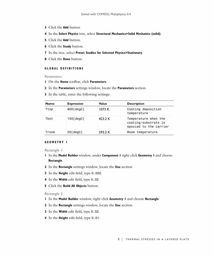
Solved with COMSOL Multiphysics 4.4
3 Click the Add button.
4 In the Select Physics tree, select Structural Mechanics>Solid Mechanics (solid).
5 Click the Add button.
6 Click the Study button.
7 In the tree, select Preset Studies for Selected Physics>Stationary.
8 Click the Done button.
G L O B A L D E F I N I T I O N S
Parameters1 On the Home toolbar, click Parameters.
2 In the Parameters settings window, locate the Parameters section.
3 In the table, enter the following settings:
G E O M E T R Y 1
Rectangle 11 In the Model Builder window, under Component 1 right-click Geometry 1 and choose
Rectangle.
2 In the Rectangle settings window, locate the Size section.
3 In the Height edit field, type 0.002.
4 In the Width edit field, type 0.02.
5 Click the Build All Objects button.
Rectangle 21 In the Model Builder window, right-click Geometry 1 and choose Rectangle.
2 In the Rectangle settings window, locate the Size section.
3 In the Width edit field, type 0.02.
4 In the Height edit field, type 0.01.
Name Expression Value Description
Ttop 800[degC] 1073 K Coating deposition temperature
Tbot 150[degC] 423.2 K Temperature when the coating/substrate is epoxied to the carrier
Troom 20[degC] 293.2 K Room temperature
5 | T H E R M A L S T R E S S E S I N A L A Y E R E D P L A T E

Solved with COMSOL Multiphysics 4.4
6 | T H E
5 Locate the Position section. In the y edit field, type 0.002.
6 Click the Build All Objects button.
Rectangle 31 Right-click Geometry 1 and choose Rectangle.
2 In the Rectangle settings window, locate the Size section.
3 In the Width edit field, type 0.02.
4 In the Height edit field, type 0.002.
5 Locate the Position section. In the y edit field, type 0.012.
6 Click the Build All Objects button.
7 Click the Zoom Extents button on the Graphics toolbar.
S O L I D M E C H A N I C S
1 In the Model Builder window, under Component 1 right-click Solid Mechanics and choose Rename.
2 Go to the Rename Solid Mechanics dialog box and type Two Layers in the New name edit field.
3 Click OK.
4 Select Domains 2 and 3 only.
TW O L A Y E R S
Linear Elastic Material 1In the Model Builder window, expand the Component 1>Two Layers node.
Thermal Expansion 11 Right-click Linear Elastic Material 1 and choose Thermal Expansion.
2 In the Thermal Expansion settings window, locate the Thermal Expansion Properties section.
3 In the Tref edit field, type Ttop.
4 Locate the Model Inputs section. In the T edit field, type Tbot.
Fixed Constraint 11 On the Physics toolbar, click Points and choose Fixed Constraint.
2 Select Point 4 only.
Prescribed Displacement 11 On the Physics toolbar, click Points and choose Prescribed Displacement.
R M A L S T R E S S E S I N A L A Y E R E D P L A T E

Solved with COMSOL Multiphysics 4.4
2 Select Point 8 only.
3 In the Prescribed Displacement settings window, locate the Prescribed Displacement section.
4 Select the Prescribed in y direction check box.
S O L I D M E C H A N I C S 2
1 In the Model Builder window, under Component 1 right-click Solid Mechanics 2 and choose Rename.
2 Go to the Rename Solid Mechanics dialog box and type Three Layers in the New
name edit field.
3 Click OK.
T H R E E L A Y E R S
Thermal Expansion 11 In the Model Builder window, under Component 1>Three Layers right-click Linear
Elastic Material 1 and choose Thermal Expansion.
2 In the Thermal Expansion settings window, locate the Thermal Expansion Properties section.
3 In the Tref edit field, type Tbot.
4 Locate the Model Inputs section. In the T edit field, type Troom.
Fixed Constraint 11 On the Physics toolbar, click Points and choose Fixed Constraint.
2 Select Point 4 only.
Prescribed Displacement 11 On the Physics toolbar, click Points and choose Prescribed Displacement.
2 Select Point 8 only.
3 In the Prescribed Displacement settings window, locate the Prescribed Displacement section.
4 Select the Prescribed in y direction check box.
Linear Elastic Material 1Use the stresses from the two layer model as initial stresses for the three layer model.
Initial Stress and Strain 11 Right-click Linear Elastic Material 1 and choose Initial Stress and Strain.
7 | T H E R M A L S T R E S S E S I N A L A Y E R E D P L A T E

Solved with COMSOL Multiphysics 4.4
8 | T H E
2 Select Domains 2 and 3 only.
3 In the Initial Stress and Strain settings window, locate the Initial Stress and Strain section.
4 In the S0 table, enter the following settings:
M A T E R I A L S
Material 11 In the Model Builder window, under Component 1 right-click Materials and choose
New Material.
2 Right-click Material 1 and choose Rename.
3 Go to the Rename Material dialog box and type Carrier in the New name edit field.
4 Click OK.
5 In the Material settings window, locate the Geometric Entity Selection section.
6 From the Selection list, choose Manual.
7 Click Clear Selection.
8 Select Domain 1 only.
9 Locate the Material Contents section. In the table, enter the following settings:
Material 21 In the Model Builder window, right-click Materials and choose New Material.
2 Right-click Material 2 and choose Rename.
3 Go to the Rename Material dialog box and type Substrate in the New name edit field.
solid.sx solid.sxy 0
solid.sxy solid.sy 0
0 0 solid.sz
Property Name Value Unit Property group
Young's modulus E 2.15e11
Pa Basic
Poisson's ratio nu 0.3 1 Basic
Density rho 1000 kg/m³ Basic
Coefficient of thermal expansion
alpha 6e-6 1/K Basic
R M A L S T R E S S E S I N A L A Y E R E D P L A T E

Solved with COMSOL Multiphysics 4.4
4 Click OK.
5 Select Domain 2 only.
6 In the Material settings window, locate the Material Contents section.
7 In the table, enter the following settings:
Material 31 In the Model Builder window, right-click Materials and choose New Material.
2 Right-click Material 3 and choose Rename.
3 Go to the Rename Material dialog box and type Coating in the New name edit field.
4 Click OK.
5 Select Domain 3 only.
6 In the Material settings window, locate the Material Contents section.
7 In the table, enter the following settings:
M E S H 1
Size1 In the Model Builder window, under Component 1 right-click Mesh 1 and choose
Mapped.
2 In the Size settings window, locate the Element Size section.
3 From the Predefined list, choose Extra fine.
4 Click the Build All button.
Property Name Value Unit Property group
Young's modulus E 1.3e11 Pa Basic
Poisson's ratio nu 0.28 1 Basic
Density rho 1000 kg/m³ Basic
Coefficient of thermal expansion
alpha 3e-6 1/K Basic
Property Name Value Unit Property group
Young's modulus E 7e10 Pa Basic
Poisson's ratio nu 0.17 1 Basic
Density rho 1000 kg/m³ Basic
Coefficient of thermal expansion
alpha 5e-7 1/K Basic
9 | T H E R M A L S T R E S S E S I N A L A Y E R E D P L A T E

Solved with COMSOL Multiphysics 4.4
10 | T H
S T U D Y 1
Add a static solution for the case with three layers.
Step 2: Stationary 21 On the Study toolbar, click Study Steps and choose Stationary>Stationary.
Use only one Solid Mechanics interface per solution by deactivating the other one.
Step 1: Stationary2 In the Model Builder window, under Study 1 click Step 1: Stationary.
3 In the Stationary settings window, locate the Physics and Variables Selection section.
4 In the table, enter the following settings:
Step 2: Stationary 25 In the Model Builder window, under Study 1 click Step 2: Stationary 2.
6 In the Stationary settings window, locate the Physics and Variables Selection section.
7 In the table, enter the following settings:
8 On the Home toolbar, click Compute.
R E S U L T S
Stress (solid)1 In the Model Builder window, expand the Stress (solid) node, then click Surface 1.
2 In the Surface settings window, click Replace Expression in the upper-right corner of the Expression section. From the menu, choose Two Layers>Stress>Stress tensor
(Spatial)>Stress tensor, x component (solid.sx).
3 On the 2D plot group toolbar, click Plot.
4 Click the Zoom Extents button on the Graphics toolbar.
Stress (solid2)1 In the Model Builder window, under Results>Stress (solid2) click Surface 1.
Physics Solve for Discretization
Three Layers × Physics Settings
Physics Solve for Discretization
Two Layers × Physics Settings
E R M A L S T R E S S E S I N A L A Y E R E D P L A T E

Solved with COMSOL Multiphysics 4.4
2 In the Surface settings window, click Replace Expression in the upper-right corner of the Expression section. From the menu, choose Three Layers>Stress>Stress tensor
(Spatial)>Stress tensor, x component (solid2.sx).
3 On the 2D plot group toolbar, click Plot.
11 | T H E R M A L S T R E S S E S I N A L A Y E R E D P L A T E

Solved with COMSOL Multiphysics 4.4
12 | T H
E R M A L S T R E S S E S I N A L A Y E R E D P L A T E
Solved with COMSOL Multiphysics 4.4
Non l i n e a r Magn e t o s t r i c t i v e T r a n s du c e r
Introduction
Magnetostriction describes the change in dimensions of a material due to a change in its magnetization. This phenomenon is a manifestation of magnetoelastic coupling, which is exhibited by all magnetic materials to some extent. The effects related to magnetoelastic coupling are described by various names. The Joule effect describes the change in length due to a change in the magnetization state of the material. This phenomenon is also known as linear magnetostriction and assumes that the volume of the material remains constant. The magnetostrictive effect is used in transducers for applications in sonars, acoustic devices, active vibration control, position control, and fuel injection systems.
Magnetostriction has a quantum-mechanical origin. The magneto-mechanical coupling takes place at the atomic level due to spin-orbit coupling. From a system level, the material can be assumed to consist of a number of tiny ellipsoidal magnets which rotate due to the torque produced by the externally applied magnetic field. The rotation of these elemental magnets produces a dimensional change leading to free strain in the material. The free strain () is often modeled using the linear constitutive relation (dH) where d is a piezo-magnetic strain coefficient and H is the magnetic field. In reality, the free strain (magnetostriction) has a nonlinear dependence on the magnetic field and the mechanical stress in the material.
This tutorial demonstrates how to model the nonlinear magnetostrictive response of a magnetostrictive material using the nonlinear HB curve data of that material. The effect of stress on magnetostriction will not be explicitly modeled. It is assumed that the nonlinear HB curve used is obtained under an iso-stress condition and that the stress state of the material considered in this model is the same as that for which the HB curve was obtained.
Model Definition
In this tutorial you will model a typical magnetostrictive transducer shown in Figure 1.The transducer has a steel housing enclosing a drive coil. A magnetostrictive
1 | N O N L I N E A R M A G N E T O S T R I C T I V E TR A N S D U C E R

Solved with COMSOL Multiphysics 4.4
2 | N O N
material is placed in the core which works as an actuator when a magnetic field is produced by passing a current through the drive coil.
Figure 1: Sectional view of a cylindrical transducer.
Due to the symmetric nature of the geometry the problem will be solved as a 2D axisymmetric model. This will lead to reduced computation time. The corresponding 2D axisymmetric geometry is shown in Figure 2.
Figure 2: 2D axisymmetric view of a magnetostrictive transducer surrounded by an air domain. The geometric dimensions are in millimeters.
L I N E A R M A G N E T O S T R I C T I V E TR A N S D U C E R

Solved with COMSOL Multiphysics 4.4
It is assumed that the current in the coil is DC and hence this model can be solved as a stationary problem. The first study performed considers a constant current density of 106 A/m2 in the coil. A second study is set up where the current density in the drive coil is varied from 0 to 107 A/m2 using the parametric sweep feature in COMSOL. The solution from this parametric sweep is then used to generate the characteristic nonlinear magnetostriction () vs. magnetic field (H) curve. The ramping of current density using the parametric sweep option is performed under the assumption that the current in the coil changes quasi-statically without producing any inductive effect.
N O T E S O N T H E M A G N E T I C P R O B L E M
An air domain is created around the transducer to realistically model the magnetic flux path. The boundaries of this air domain are magnetically insulated which ensures that flux does not diverge out of the modeling domain. An alternate technique of implementing this air domain in COMSOL involves the use of Infinite Elements. For more information on Infinite Elements, please refer to the AC/DC Module User’s Guide.
The drive coil is modeled as a homogenized current carrying domain. Individual wires and their electrical conductivity are not resolved. It is assumed that the externally applied current density in the coil is known a priori. In a 2D axisymmetric model, the external current density is the total current through the coil divided by the longitudinal cross-section area (coil length times coil thickness). The coil can also be modeled alternately using the Multiturn Coil Domain feature available in the AC/DC Module. Please refer to the AC/DC Module User’s Guide for more details on using this alternative technique.
The steel housing used in this example is designed to create a closed magnetic flux path thereby minimizing flux leakage. The nonlinear magnetic behavior of the steel housing is modeled by using a HB curve to specify the magnetic constitutive relation in the steel housing. The nonlinear HB curve used is obtained by choosing the material Soft iron without losses from AC/DC materials in COMSOL’s Material Browser. Incorporation of a nonlinear HB curve helps in modeling magnetic saturation effects at sufficiently high magnetic field. Furthermore, you can examine the results of the model to find out specific locations in a material where magnetic saturation has taken place whereas other regions of that material have remained unsaturated. Using finite element analysis enables us to resolve such material nonlinearity over space thereby helping us in device design optimization.
In the same manner as mentioned above a nonlinear HB relation is also used for the magnetostrictive material. The HB data for the magnetostrictive material is available in
3 | N O N L I N E A R M A G N E T O S T R I C T I V E TR A N S D U C E R
Solved with COMSOL Multiphysics 4.4
4 | N O N
a text file. This text file is read into COMSOL and is used to create an interpolation function that can provide a value of the magnetic field (H) for a given magnetic flux density (B) in the material. Although traditionally the B-field is obtained as a function of the H-field, in COMSOL you need to specify the other way round while working with the built-in magnetic fields interface. The reason why you need an HB curve is that the vector formulation of the magnetic problem in COMSOL Multiphysics solves for the magnetic vector potential A whose curl yields the vector B-field or magnetic flux density. The H-field is then obtained as a function of the B-field. Hence, in order to avoid circular dependency it is necessary to specify the H-field in terms of the B-field.
The other material properties used to describe the magnetostrictive material are shown in Table 1.
In this model you can assume the electric conductivity of the magnetostrictive material to be zero because you are working with magnetic fields produced by DC currents in the coil and hence you do not have to model eddy currents in the magnetostrictive material.
C A L C U L A T I N G N O N L I N E A R M A G N E T O S T R I C T I O N
The magnetostriction component along any direction can be calculated as a nonlinear function of the magnetization using Equation 1 (Ref. 1).
(1)
Magnetostriction () along the direction i depends on the magnetostriction constant (s) and the magnetization direction cosine (i). The direction cosine is the ratio of magnetization along the required direction (Mi) and the saturation magnetization (Ms) of the material. The negative 13 term indicates that the magnetic moments are
TABLE 1: MATERIAL PROPERTIES OF THE MAGNETOSTRICTIVE MATERIAL
MATERIAL PROPERTY VALUE DESCRIPTION
E 60.109 Pa Young’s modulus
0.45 Poisson’s ratio
7870 kg/m3 Density
0 Electric conductivity
r 1 Relative permittivity
s 2.10-4 Magnetostriction constant
Msat 15.105 A/m Saturation magnetization
i32---s i
2 13---–
32---s
MiMs-------
2 13---–= =
L I N E A R M A G N E T O S T R I C T I V E TR A N S D U C E R

Solved with COMSOL Multiphysics 4.4
randomly oriented in the material in the absence of any magnetic field. In this tutorial you will not use the negative 13 term because of the assumption that the material is sufficiently prestressed such that all magnetic moments are perpendicular to the direction of magnetization at the beginning of the magnetization process. The material in a prestressed state would yield maximum magnetostriction (Ref. 1).
The next step is to incorporate the free strain due to magnetostriction in the structural part of the model.
C O U P L I N G T H E M A G N E T I C A N D S T R U C T U R A L P R O B L E M S
The objective of this tutorial is to understand the mechanism of modeling nonlinear magnetostriction and hence the structural problem is solved only in the magnetostrictive material. A detailed design of the transducer could involve the modeling of more mechanisms. For example, the lower surface of the magnetostrictive rod could be rigidly fastened to the base plate of the housing using either bolted or welded joints. Similarly the upper surface of the rod could be connected to a piston that could work like a plunger due to the actuation effect. Typically this piston would be connected to other lever mechanisms or valves which would be actuated using the magnetostrictive strain. In this tutorial you will not model these case-specific detailed mechanisms. The only interaction that is taken into account is that between the lower edge of the magnetostrictive material and the base plate of the steel housing which is implemented by using a fixed constraint boundary condition on the lower edge of the magnetostrictive material.
The free strain due to magnetostriction is incorporated using an extension of the Hooke’s Law. COMSOL uses a generalized Hooke’s Law to describe the constitutive relationship between the stress and strain tensors in a solid mechanics problem. This general form of the linear constitutive relation allows the incorporation of initial strain in a material which does not contribute to mechanical stress unless the material is mechanically constrained. Because, by definition, the magnetostriction or magnetization-induced free strain in the material is equivalent to an initial strain, this idea is used to incorporate the magnetostriction calculated from Equation 1.
Note that although you use the linear elastic material model, you can still incorporate nonlinear strains in a material using the option to add initial strain. More information on the constitutive relation used in COMSOL for linear elastic material and the initial strain term in this relation can be obtained from the Structural Mechanics Module User’s Guide.
In a 2D axisymmetric model, you need to consider radial, azimuthal, and axial strain components. However, because the azimuthal magnetic field is zero due to the
5 | N O N L I N E A R M A G N E T O S T R I C T I V E TR A N S D U C E R

Solved with COMSOL Multiphysics 4.4
6 | N O N
orientation of the drive coil, you can consider the azimuthal magnetostriction to be zero as well. In this model, the dominant magnetostriction component is along the Z direction. For consistency the radial component of magnetostriction is also calculated and incorporated as initial strain.
Results and Discussion
The results obtained from the first study where a constant external current density of 106 A/m2 is applied to the coil are shown in Figure 3. The solution shows magnetic flux concentration in the magnetostrictive core due to the closed magnetic path provided by the steel housing. The magnetic flux density in the rod is mostly uniform and its magnitude is around 1.5 T. Fringe effects can be seen at the two ends of the rod where majority of the magnetic flux is forced to curl into the steel housing.
Figure 3: Surface plot of the norm of the magnetic flux density and a normalized arrow plot of its r and z-components showing the closed flux path in the model.
Figure 4 shows the z-component of stress in the magnetostrictive material as a surface plot. This plot shows that the stress due to magnetostriction is uniformly zero in the material as the free strain due to magnetostriction should not produce any stress unless the material is mechanically constrained. A local stress concentration effect can be observed near the bottom surface of the rod due to the fixed constraint boundary condition that was applied to this end of the rod.
L I N E A R M A G N E T O S T R I C T I V E TR A N S D U C E R

Solved with COMSOL Multiphysics 4.4
Figure 4: Surface plot of the z-component of stress and a scaled deformation plot of the displacement.
Figure 5 shows the z-component of strain in the magnetostrictive material as a surface plot. This plot shows that the dominant strain component due to magnetostriction is fairly uniform in the material except at the two ends of the rod due to fringe effect. Note that the magnetic field changes direction at the ends of the rod as most of the magnetic flux is concentrated through the steel housing.
7 | N O N L I N E A R M A G N E T O S T R I C T I V E TR A N S D U C E R

Solved with COMSOL Multiphysics 4.4
8 | N O N
Figure 5: Surface plot of the z-component of strain.
Figure 6 shows an interesting postprocessing feature in COMSOL. The solution obtained from the 2D axisymmetric model has been revolved by 225 degrees for 3D visualization of the solution. On solving a 2D axisymmetry model, COMSOL automatically creates a 3D solution data set by revolving the solution which is then plotted as a 3D plot. Figure 6 shows a volume plot of the norm of the magnetic flux density in the region inside the transducer housing including the magnetostrictive core. The solution in the region outside the housing (that is, the air domain) has been suppressed using a filter. A normalized arrow plot shows the magnetic flux path.
L I N E A R M A G N E T O S T R I C T I V E TR A N S D U C E R

Solved with COMSOL Multiphysics 4.4
Figure 6: A 225 degree sectional view in 3D of the norm of the magnetic flux density in the magnetostrictive rod, steel housing and in the region within the housing. The solution in the outer air domain has been suppressed to get a better view. The normalized arrow plot shows the direction of the magnetic flux density.
Figure 7 shows the characteristic H curve of the magnetostrictive material obtained from the parametric study that simulated a quasi-static ramping up of the current density in the coil. Because the magnetic field is oriented mostly along the axial direction (Z direction), only the Z-components of the magnetostriction and magnetic field are plotted. Note the sharp nonlinear behavior in the region where the magnetic field Hz varies between 0 to 2.104 A/m. The onset of saturation is observed beyond a magnetic field of 3.104 A/m.
Figure 8 shows the Z-displacement (w) versus the external current density applied to the drive coil. This is often more useful for determining the performance of a transducer. The same nonlinearity and saturation effect in the performance as shown in Figure 7 can be observed here as well.
9 | N O N L I N E A R M A G N E T O S T R I C T I V E TR A N S D U C E R

Solved with COMSOL Multiphysics 4.4
10 | N O
Figure 7: Magnetostriction () versus Magnetic field (H) curve at a point on the magnetostrictive material.
Figure 8: Z-displacement (w) versus External current density (J) curve at a point on the magnetostrictive material.
N L I N E A R M A G N E T O S T R I C T I V E TR A N S D U C E R

Solved with COMSOL Multiphysics 4.4
Reference
1. S. Chikazumi, Physics of Ferromagnetism, Oxford University Press, New York, 1997.
Model Library path: Structural_Mechanics_Module/Magnetostrictive_Devices/nonlinear_magnetostriction
Modeling Instructions
From the File menu, choose New.
N E W
1 In the New window, click the Model Wizard button.
M O D E L W I Z A R D
1 In the Model Wizard window, click the 2D Axisymmetric button.
2 In the Select physics tree, select AC/DC>Magnetic Fields (mf).
3 Click the Add button.
4 In the Select physics tree, select Structural Mechanics>Solid Mechanics (solid).
5 Click the Add button.
6 Click the Study button.
7 In the tree, select Preset Studies for Selected Physics>Stationary.
8 Click the Done button.
G E O M E T R Y 1
1 In the Model Builder window, under Component 1 click Geometry 1.
2 In the Geometry settings window, locate the Units section.
3 From the Length unit list, choose mm.
Rectangle 11 Right-click Component 1>Geometry 1 and choose Rectangle.
2 In the Rectangle settings window, locate the Size section.
3 In the Width edit field, type 3.
4 In the Height edit field, type 50.
11 | N O N L I N E A R M A G N E T O S T R I C T I V E TR A N S D U C E R

Solved with COMSOL Multiphysics 4.4
12 | N O
5 Locate the Position section. In the z edit field, type -25.
6 Click the Build Selected button.
Copy 11 On the Geometry toolbar, click Copy.
2 Select the object r1 only.
3 In the Copy settings window, locate the Displacement section.
4 In the r edit field, type 7.5.
5 Click the Build Selected button.
Rectangle 21 In the Model Builder window, right-click Geometry 1 and choose Rectangle.
2 In the Rectangle settings window, locate the Size section.
3 In the Width edit field, type 20.
4 In the Height edit field, type 5.
5 Locate the Position section. In the z edit field, type -30.
6 Click the Build Selected button.
Copy 21 On the Geometry toolbar, click Copy.
2 Select the object r2 only.
3 In the Copy settings window, locate the Displacement section.
4 In the z edit field, type 55.
5 Click the Build Selected button.
Rectangle 31 Right-click Geometry 1 and choose Rectangle.
2 In the Rectangle settings window, locate the Size section.
3 In the Width edit field, type 5.
4 In the Height edit field, type 50.
5 Locate the Position section. In the r edit field, type 15.
6 In the z edit field, type -25.
7 Click the Build Selected button.
Rectangle 41 Right-click Geometry 1 and choose Rectangle.
N L I N E A R M A G N E T O S T R I C T I V E TR A N S D U C E R

Solved with COMSOL Multiphysics 4.4
2 In the Rectangle settings window, locate the Size section.
3 In the Width edit field, type 90.
4 In the Height edit field, type 180.
5 Locate the Position section. In the z edit field, type -90.
6 Click the Build Selected button.
7 Click the Zoom Extents button on the Graphics toolbar.[
This figure shows the geometric objects that need to be selected in the next step.
Union 11 On the Geometry toolbar, click Union.
2 Select the objects r3, r2, and copy2 only.
3 In the Union settings window, locate the Union section.
4 Clear the Keep interior boundaries check box.
5 Click the Build All Objects button.
6 Click the Zoom Extents button on the Graphics toolbar.
G L O B A L D E F I N I T I O N S
Parameters1 On the Home toolbar, click Parameters.
2 In the Parameters settings window, locate the Parameters section.
13 | N O N L I N E A R M A G N E T O S T R I C T I V E TR A N S D U C E R

Solved with COMSOL Multiphysics 4.4
14 | N O
3 In the table, enter the following settings:
D E F I N I T I O N S
Variables 11 In the Model Builder window, under Component 1 right-click Definitions and choose
Variables.
2 In the Variables settings window, locate the Geometric Entity Selection section.
3 From the Geometric entity level list, choose Domain.
4 Select Domain 3 only.
5 Locate the Variables section. In the table, enter the following settings:
M A T E R I A L S
On the Home toolbar, click Add Material.
A D D M A T E R I A L
1 Go to the Add Material window.
2 In the tree, select Built-In>Air.
3 In the Add material window, click Add to Component.
M A T E R I A L S
Air1 In the Model Builder window, under Component 1>Materials click Air.
2 Select Domains 1 and 4–6 only.
Name Expression Value Description
Msat 1.5e6[A/m] 1.500E6 A/m Saturation magnetization
Lambda_s 200e-6 2.000E-4 Magnetostriction constant
J0 1e6[A/m^2] 1.000E6 A/m² Current density
Name Expression Unit Description
Lambda_r 1.5*Lambda_s*(mf.Mr/Msat)^2
Magnetostriction along radial direction
Lambda_z 1.5*Lambda_s*(mf.Mz/Msat)^2
Magnetostriction along axial direction
N L I N E A R M A G N E T O S T R I C T I V E TR A N S D U C E R

Solved with COMSOL Multiphysics 4.4
A D D M A T E R I A L
1 Go to the Add Material window.
2 In the tree, select AC/DC>Soft Iron (without losses).
3 In the Add material window, click Add to Component.
M A T E R I A L S
Soft Iron (without losses)1 In the Model Builder window, under Component 1>Materials click Soft Iron (without
losses).
2 In the Material settings window, locate the Geometric Entity Selection section.
3 Click Paste Selection.
4 Go to the Paste Selection dialog box.
5 In the Selection edit field, type 2.
6 Click the OK button.
7 On the Home toolbar, click Add Material.
Material 31 In the Model Builder window, right-click Materials and choose New Material.
2 Select Domain 3 only.
3 In the Material settings window, locate the Material Contents section.
4 In the table, enter the following settings:
5 Click to expand the Material properties section. Locate the Material Properties section. In the Material properties tree, select Electromagnetic Models>HB Curve.
6 Click Add to Material.
Interpolation 11 On the Home toolbar, click Functions and choose Global>Interpolation.
Property Name Value Unit Property group
Electrical conductivity sigma 0 S/m Basic
Relative permittivity epsilonr
1 1 Basic
Young's modulus E 60e9 Pa Basic
Poisson's ratio nu 0.45 1 Basic
Density rho 7870 kg/m³ Basic
15 | N O N L I N E A R M A G N E T O S T R I C T I V E TR A N S D U C E R

Solved with COMSOL Multiphysics 4.4
16 | N O
2 In the Interpolation settings window, locate the Definition section.
3 From the Data source list, choose File.
4 Find the Functions subsection. Click the Browse button.
5 Browse to the model’s Model Library folder and double-click the file nonlinear_magnetostriction_HBFe.txt.
6 Click the Import button.
7 In the Function name edit field, type HB.
Material 31 In the Model Builder window, under Component 1>Materials click Material 3.
2 In the Material settings window, locate the Material Contents section.
3 In the table, enter the following settings:
4 Right-click Component 1>Materials>Material 3 and choose Rename.
5 Go to the Rename Material dialog box and type Magnetostrictive in the New name edit field.
6 Click OK.
M A G N E T I C F I E L D S
Ampère's Law 21 On the Physics toolbar, click Domains and choose Ampère's Law.
2 Select Domains 2 and 3 only.
3 In the Ampère's Law settings window, locate the Magnetic Field section.
4 From the Constitutive relation list, choose HB curve.
External Current Density 11 On the Physics toolbar, click Domains and choose External Current Density.
2 Select Domain 5 only.
3 In the External Current Density settings window, locate the External Current Density section.
Property Name Value Unit Property group
Magnetic field norm normH
HB(normB[1/T])[A/m]
A/m HB curve
N L I N E A R M A G N E T O S T R I C T I V E TR A N S D U C E R

Solved with COMSOL Multiphysics 4.4
4 Specify the Je vector as
S O L I D M E C H A N I C S
1 In the Model Builder window, under Component 1 click Solid Mechanics.
2 In the Solid Mechanics settings window, locate the Domain Selection section.
3 Click Clear Selection.
4 Select Domain 3 only.
The solid mechanics equations will be solved only in the magnetostrictive material.
Initial Stress and Strain 11 In the Model Builder window, under Component 1>Solid Mechanics right-click Linear
Elastic Material 1 and choose Initial Stress and Strain.
2 In the Initial Stress and Strain settings window, locate the Initial Stress and Strain section.
3 In the 0 table, enter the following settings:
Fixed Constraint 11 On the Physics toolbar, click Boundaries and choose Fixed Constraint.
2 Select Boundary 6 only.
This boundary condition simulates that the lower surface of the magnetostrictive rod is fixed to the base of the transducer housing.
M E S H 1
Free Triangular 1In the Model Builder window, under Component 1 right-click Mesh 1 and choose Free Triangular.
0 r
J0 phi
0 z
Lambda_r 0 0
0 0 0
0 0 Lambda_z
17 | N O N L I N E A R M A G N E T O S T R I C T I V E TR A N S D U C E R

Solved with COMSOL Multiphysics 4.4
18 | N O
Size 11 In the Model Builder window, under Component 1>Mesh 1 right-click Free Triangular
1 and choose Size.
2 In the Size settings window, locate the Geometric Entity Selection section.
3 From the Geometric entity level list, choose Domain.
4 Select Domains 2 and 3 only.
5 Locate the Element Size section. Click the Custom button.
6 Locate the Element Size Parameters section. Select the Maximum element size check box.
7 In the associated edit field, type 0.5.
These settings create a significantly more refined mesh in the nonlinear magnetic material, which is useful for resolving the spatial distribution of material nonlinearity.
8 Click the Build All button.
S T U D Y 1
On the Home toolbar, click Compute.
R E S U L T S
Magnetic Flux Density Norm (mf)Follow the steps below to create Figure 3 to Figure 5.
1 In the Model Builder window, right-click Magnetic Flux Density Norm (mf) and choose Arrow Surface.
The default expression in the arrow surface plot creates an arrow plot of the R- and Z-components of the magnetic flux density.
2 In the Arrow Surface settings window, locate the Arrow Positioning section.
3 In the Points edit field, type 20.
4 Locate the Coloring and Style section. From the Color list, choose White.
5 From the Arrow length list, choose Normalized.
The plot in the Graphics window should look like that in Figure 3.
Stress (solid)The second default surface plot shows the von Mises stress in the magnetostrictive core along with a scaled deformation plot.
N L I N E A R M A G N E T O S T R I C T I V E TR A N S D U C E R

Solved with COMSOL Multiphysics 4.4
1 In the Model Builder window, expand the Results>Stress (solid) node, then click Surface 1.
2 In the Surface settings window, click Replace Expression in the upper-right corner of the Expression section. From the menu, choose Solid Mechanics>Stress>Stress tensor
(Spatial)>Stress tensor, z component (solid.sz).
3 On the Stress (solid) toolbar, click Plot.
Compare with the plot in Figure 4.
2D Plot Group 51 On the Home toolbar, click Add Plot Group and choose 2D Plot Group.
2 In the Model Builder window, under Results right-click 2D Plot Group 5 and choose Surface.
3 In the Surface settings window, click Replace Expression in the upper-right corner of the Expression section. From the menu, choose Solid Mechanics>Strain>Strain tensor
(Material)>Strain tensor, ZZ component (solid.eZZ).
4 On the 2D Plot Group 5 toolbar, click Plot.
5 In the Model Builder window, right-click 2D Plot Group 5 and choose Rename.
6 Go to the Rename 2D Plot Group dialog box and type Strain (solid) in the New
name edit field.
7 Click OK.
Compare the resulting plot with that in Figure 5.
Follow the steps outlined below to create Figure 6.
3D Plot Group 61 On the Home toolbar, click Add Plot Group and choose 3D Plot Group.
2 In the Model Builder window, under Results right-click 3D Plot Group 6 and choose Volume.
3 Right-click Results>3D Plot Group 6>Volume 1 and choose Filter.
4 In the Filter settings window, locate the Element Selection section.
5 In the Logical expression for inclusion edit field, type dom!=1.
This excludes the outer air domain from the plot.
6 On the 3D Plot Group 6 toolbar, click Plot.
7 In the Model Builder window, right-click 3D Plot Group 6 and choose Arrow Volume.
8 In the Arrow Volume settings window, locate the Expression section.
19 | N O N L I N E A R M A G N E T O S T R I C T I V E TR A N S D U C E R

Solved with COMSOL Multiphysics 4.4
20 | N O
9 In the X component edit field, type mf.Br*cos(rev1phi)-mf.Bphi*sin(rev1phi).
10 In the Y component edit field, type mf.Br*sin(rev1phi)+mf.Bphi*cos(rev1phi).
11 Locate the Arrow Positioning section. From the Entry method list, choose Coordinates.
12 In the Coordinates edit field, type range(-20,4,20).
13 From the Entry method list, choose Coordinates.
14 In the Coordinates edit field, type range(-20,4,20).
15 From the Entry method list, choose Coordinates.
16 In the Coordinates edit field, type range(-30,2.5,30).
17 Locate the Coloring and Style section. From the Arrow length list, choose Normalized.
18 Select the Scale factor check box.
19 In the associated edit field, type 3.
20 On the 3D Plot Group 6 toolbar, click Plot.
21 Click the Zoom In button on the Graphics toolbar.
22 Click the Zoom In button on the Graphics toolbar.
23 Right-click 3D Plot Group 6 and choose Rename.
24 Go to the Rename 3D Plot Group dialog box and type Magnetic Flux Density, 3D (mf) in the New name edit field.
25 Click OK.
Next, perform a auxiliary continuation sweep on the external current density and plot the solution to view the saturation effect in the magnetostrictive core.
R O O T
On the Home toolbar, click Add Study.
A D D S T U D Y
1 Go to the Add Study window.
2 Find the Studies subsection. In the tree, select Preset Studies>Stationary.
3 In the Add study window, click Add Study.
4 On the Home toolbar, click Add Study.
N L I N E A R M A G N E T O S T R I C T I V E TR A N S D U C E R

Solved with COMSOL Multiphysics 4.4
S T U D Y 2
Step 1: Stationary1 In the Model Builder window, under Study 2 click Step 1: Stationary.
2 In the Stationary settings window, click to expand the Study extensions section.
3 Locate the Study Extensions section. Select the Auxiliary sweep check box.
4 Click Add.
5 In the table, enter the following settings:
6 Click Range.
7 Go to the Range dialog box.
8 From the Entry method list, choose Number of values.
9 In the Start edit field, type 0.
10 In the Stop edit field, type 7.
11 In the Number of values edit field, type 50.
12 From the Function to apply to all values list, choose exp10.
13 Click the Add button.
Running the entire parametric study based on the settings above will take several minutes. The exact solution time will vary depending on the specification of the computer being used.
14 On the Home toolbar, click Compute.
R E S U L T S
Magnetic Flux Density Norm (mf) 2Follow the instructions below to create Figure 7 and Figure 8.
1D Plot Group 111 On the Home toolbar, click Add Plot Group and choose 1D Plot Group.
2 In the 1D Plot Group settings window, locate the Data section.
3 From the Data set list, choose Solution 2.
4 Click to expand the Title section. From the Title type list, choose Manual.
5 In the Title text area, type Magnetostriction curve.
Auxiliary parameter Parameter value list
J0
21 | N O N L I N E A R M A G N E T O S T R I C T I V E TR A N S D U C E R

Solved with COMSOL Multiphysics 4.4
22 | N O
6 Locate the Plot Settings section. Select the x-axis label check box.
7 In the associated edit field, type Magnetic field (A/m).
8 Select the y-axis label check box.
9 In the associated edit field, type Magnetostriction.
10 On the 1D Plot Group 11 toolbar, click Point Graph.
11 In the Point Graph settings window, locate the Selection section.
12 Click Paste Selection.
13 Go to the Paste Selection dialog box.
14 In the Selection edit field, type 8.
15 Click the OK button.
16 In the Point Graph settings window, click Replace Expression in the upper-right corner of the y-axis data section. From the menu, choose Definitions>Magnetostriction along axial direction (Lambda_z).
17 Locate the x-Axis Data section. From the Parameter list, choose Expression.
18 Click Replace Expression in the upper-right corner of the x-axis data section. From the menu, choose Magnetic Fields>Magnetic>Magnetic field (Spatial)>Magnetic field, z
component (mf.Hz).
19 On the 1D Plot Group 11 toolbar, click Plot.
20 In the Model Builder window, right-click 1D Plot Group 11 and choose Rename.
21 Go to the Rename 1D Plot Group dialog box and type Magnetostriction in the New
name edit field.
22 Click OK.
1D Plot Group 121 On the Home toolbar, click Add Plot Group and choose 1D Plot Group.
2 In the 1D Plot Group settings window, locate the Data section.
3 From the Data set list, choose Solution 2.
4 Locate the Title section. From the Title type list, choose Manual.
5 In the Title text area, type Current-Displacement curve.
6 Locate the Plot Settings section. Select the x-axis label check box.
7 In the associated edit field, type Current density (A/m<sup>2</sup>).
8 Select the y-axis label check box.
9 In the associated edit field, type Displacement (mm).
N L I N E A R M A G N E T O S T R I C T I V E TR A N S D U C E R

Solved with COMSOL Multiphysics 4.4
10 On the 1D Plot Group 12 toolbar, click Point Graph.
11 In the Point Graph settings window, locate the Selection section.
12 Click Paste Selection.
13 Go to the Paste Selection dialog box.
14 In the Selection edit field, type 8.
15 Click the OK button.
16 In the Point Graph settings window, click Replace Expression in the upper-right corner of the y-axis data section. From the menu, choose Solid
Mechanics>Displacement>Displacement field (Material)>Displacement field, Z
component (w).
17 On the 1D Plot Group 12 toolbar, click Plot.
18 In the Model Builder window, right-click 1D Plot Group 12 and choose Rename.
19 Go to the Rename 1D Plot Group dialog box and type Current-Displacement in the New name edit field.
20 Click OK.
23 | N O N L I N E A R M A G N E T O S T R I C T I V E TR A N S D U C E R

Solved with COMSOL Multiphysics 4.4
24 | N O
N L I N E A R M A G N E T O S T R I C T I V E TR A N S D U C E R
Solved with COMSOL Multiphysics 4.4
P r a t t T r u s s B r i d g e
Introduction
This example is inspired by a classic bridge type called a Pratt truss bridge. You can identify a Pratt truss by its diagonal members, which (except for the very end ones) all slant down and in toward the center of the span. All the diagonal members are subject to tension forces only, while the shorter vertical members handle the compressive forces. Since the tension removes the buckling risk, this allows for thinner diagonal members resulting in a more economic design.
A truss structure supports only tension and compression forces in its members and you would normally model it using bars, but as this model uses 3D beams it also includes bending moments to some extent in a frame structure. In the model, shell elements represent the roadway.
Model Definition
B A S I C D I M E N S I O N S
The length of the bridge is 40 m, and the width of the roadway is 7 m. The main distance between the truss members is 5 m.
A N A L Y S I S TY P E S
The model includes two different analyses of the bridge:
• The goal of the first analysis is to evaluate the stress and deflection fields of the bridge when exposed to a pure gravity load and also when a load corresponding to one or two trucks crosses the bridge.
• Finally, an eigenfrequency analysis shows the eigenfrequencies and eigenmodes of the bridge.
L O A D S A N D C O N S T R A I N T S
To prevent rigid body motion of the bridge, it is important to constrain it properly. All translational degrees of freedom are constrained at the left-most horizontal edge. Constraints at the right-most horizontal edge prevent it from moving in the vertical and transversal directions but allow the bridge to expand or contract in the axial direction. This difference would however only be important if thermal expansion was studied.
1 | P R A T T TR U S S B R I D G E

Solved with COMSOL Multiphysics 4.4
2 | P R A
Figure 1 shows the bridge geometry.
Figure 1: The geometry of the bridge
The first study uses several load cases. In the first load case the effects of self weight are analyzed. The following load cases compute the solution when two trucks are moving over the bridge. The weight of each truck is 12,000 kg, the wheelbase is 6 m, the axle track is 2 m, and the weight is distributed with one third on the front axle and two thirds on the rear axle. The right side wheels of the truck are 1 m from the edge of the bridge.
In the second study the natural frequencies of the bridge are computed.
M A T E R I A L P R O P E R T I E S A N D C R O S S S E C T I O N D A T A
The material in the frame structure is structural steel. The roadway material is concrete; the effect of reinforcement is ignored. The frame members have different cross sections:
• The main beams along the bridge have square box profiles with height 200 mm and thickness 16 mm. This is also true for the outermost diagonal members.
T T TR U S S B R I D G E
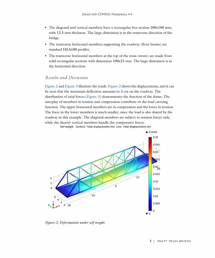
Solved with COMSOL Multiphysics 4.4
• The diagonal and vertical members have a rectangular box section 200x100 mm, with 12.5 mm thickness. The large dimension is in the transverse direction of the bridge.
• The transverse horizontal members supporting the roadway (floor beams) are standard HEA100 profiles.
• The transverse horizontal members at the top of the truss (struts) are made from solid rectangular sections with dimension 100x25 mm. The large dimension is in the horizontal direction.
Results and Discussion
Figure 2 and Figure 3 illustrate the result. Figure 2 shows the displacements, and it can be seen that the maximum deflection amounts to 3 cm on the roadway. The distribution of axial forces (Figure 3) demonstrates the function of the frame: The interplay of members in tension and compression contribute to the load carrying function. The upper horizontal members are in compression and the lower in tension. The force in the lower members is much smaller, since the load is also shared by the roadway in this example. The diagonal members are subject to tension forces only, while the shorter vertical members handle the compressive forces.
Figure 2: Deformation under self weight.
3 | P R A T T TR U S S B R I D G E

Solved with COMSOL Multiphysics 4.4
4 | P R A
Figure 3: The axial forces in the beams. Red is tension and blue is compression.
To study the effects of trucks moving over the bridge, several load cases represent the position of the trucks. The trucks are moved 3 m along the bridge for each load case. Figure 4 shows the stress distribution in the roadway when the first truck has passed
T T TR U S S B R I D G E

Solved with COMSOL Multiphysics 4.4
the bridge center and the second truck has entered the bridge deck.
Figure 4: Truck load analysis: Stresses in the bridge deck with two trucks are on the bridge.
The study of eigenfrequencies is important with respect to the excitation and frequency content from various loads such as wind loads and earthquakes.
5 | P R A T T TR U S S B R I D G E

Solved with COMSOL Multiphysics 4.4
6 | P R A
Figure 5 shows the 9th eigenmode of the bridge, which is the fundamental mode for the roadway. The first eight eigenmodes only involve displacements of the weak struts at the top of the truss.
Figure 5: The 9th eigenmode.
Notes About the COMSOL Implementation
You can define load cases to activate and deactivate loads within a study. All the loads need to be defined in the Model Builder. Under the Stationary Study node, you can then select which load or constraint to activate for a specific load case. Moreover for each load case you can modify the value of the applied load by changing its weight factor.
T T TR U S S B R I D G E

Solved with COMSOL Multiphysics 4.4
When combining two different physics interfaces, they will as a default have individual sets of degrees of freedom. In structural mechanics, you will usually want them to be equal. In this case, you add prescribed displacements to the Beam interface so that the degrees of beam degrees of freedom are set equal to the corresponding degrees of freedom from the Shell interface. The representation of rotation is however different between the two interfaces. In the example you can see how the rotations in the beam elements are prescribed to follow those in the shell by using a variable from the shell interface, rather than the degree of freedom itself. In models like this, the results will actually be virtually the same if the connection of rotations is omitted, as long as the mesh is reasonably fine.
Model Library path: Structural_Mechanics_Module/Civil_Engineering/pratt_truss_bridge
Modeling Instructions
From the File menu, choose New.
N E W
1 In the New window, click the Model Wizard button.
M O D E L W I Z A R D
1 In the Model Wizard window, click the 3D button.
2 In the Select Physics tree, select Structural Mechanics>Shell.
3 Click the Add button.
4 In the Select Physics tree, select Structural Mechanics>Beam.
5 Click the Add button.
6 Click the Study button.
7 In the tree, select Preset Studies for Selected Physics>Stationary.
8 Click the Done button.
G L O B A L D E F I N I T I O N S
Parameters1 On the Home toolbar, click Parameters.
7 | P R A T T TR U S S B R I D G E

Solved with COMSOL Multiphysics 4.4
8 | P R A
2 In the Parameters settings window, locate the Parameters section.
3 In the table, enter the following settings:
4 In the Model Builder window, right-click Global Definitions and choose Load Group. Repeat this nine times so that you get ten load groups
G E O M E T R Y 1
On the Geometry toolbar, click Work Plane.
Plane GeometryCreate the bridge deck.
Rectangle 11 In the Model Builder window, under Component 1>Geometry 1>Work Plane 1
right-click Plane Geometry and choose Rectangle.
2 In the Rectangle settings window, locate the Size section.
3 In the Width edit field, type spacing.
4 In the Height edit field, type width.
5 Locate the Position section. In the xw edit field, type -length/2.
Plane GeometryRight-click Component 1>Geometry 1>Work Plane 1>Plane Geometry>Rectangle 1 and choose Build All Objects.
Array 11 On the Work plane toolbar, click Array.
2 In the Array settings window, locate the Size section.
3 From the Array type list, choose Linear.
4 Select the object r1 only.
5 In the Size edit field, type length/spacing.
Name Expression Value Description
width 7[m] 7.000 m Width of bridge
height 5[m] 5.000 m Height of bridge
spacing 5[m] 5.000 m Spacing between members along the bridge
length 40[m] 40.00 m Total bridge length
truck_weight 12000[kg] 1.200E4 kg Total truck weight
T T TR U S S B R I D G E

Solved with COMSOL Multiphysics 4.4
6 Locate the Displacement section. In the xw edit field, type spacing.
7 Right-click Component 1>Geometry 1>Work Plane 1>Plane Geometry>Array 1 and choose Build All Objects.
8 Click the Zoom Extents button on the Graphics toolbar.
Plane GeometryMake it possible to create beams along the edges.
Convert to Curve 11 On the Work plane toolbar, click Conversions and choose Convert to Curve.
2 In the Convert to Curve settings window, locate the Input section.
3 Select the Keep input objects check box.
4 Click in the Graphics window, press Ctrl+A to highlight all objects, and then right-click to confirm the selection.
5 Right-click Component 1>Geometry 1>Work Plane 1>Plane Geometry>Convert to
Curve 1 and choose Build All Objects.
6 Right-click Geometry 1 and choose Build All Objects.
7 Click the Zoom Extents button on the Graphics toolbar.
Start creating the truss.
Work Plane 21 On the Geometry toolbar, click Work Plane.
2 In the Work Plane settings window, locate the Plane Definition section.
3 From the Plane list, choose xz-plane.
Bézier Polygon 11 In the Model Builder window, under Component 1>Geometry 1>Work Plane 2
right-click Plane Geometry and choose More Primitives>Bézier Polygon.
2 In the Bézier Polygon settings window, locate the General section.
3 From the Type list, choose Open curve.
4 Locate the Polygon Segments section. Find the Added segments subsection. Click the Add Linear button.
5 Find the Control points subsection. In row 2, set xw to spacing.
6 In row 2, set yw to height.
7 Find the Added segments subsection. Click the Add Linear button.
8 Find the Control points subsection. In row 2, set yw to 0.
9 | P R A T T TR U S S B R I D G E

Solved with COMSOL Multiphysics 4.4
10 | P R
Plane GeometryRight-click Component 1>Geometry 1>Work Plane 2>Plane Geometry>Bézier Polygon 1 and choose Build All Objects.
Bézier Polygon 21 In the Model Builder window, under Component 1>Geometry 1>Work Plane 2
right-click Plane Geometry and choose Bézier Polygon.
2 In the Bézier Polygon settings window, locate the General section.
3 From the Type list, choose Open curve.
4 Locate the Polygon Segments section. Find the Added segments subsection. Click the Add Linear button.
5 Find the Control points subsection. In row 1, set yw to height.
6 In row 2, set xw to spacing.
7 In row 2, set yw to height.
Plane GeometryRight-click Component 1>Geometry 1>Work Plane 2>Plane Geometry>Bézier Polygon 2 and choose Build All Objects.
Array 11 On the Work plane toolbar, click Array.
2 In the Array settings window, locate the Size section.
3 From the Array type list, choose Linear.
4 Select the objects b2 and b1 only.
5 In the Size edit field, type length/(2*spacing)-1.
6 Locate the Displacement section. In the xw edit field, type spacing.
Plane GeometryRight-click Component 1>Geometry 1>Work Plane 2>Plane Geometry>Array 1 and choose Build All Objects.
Bézier Polygon 31 In the Model Builder window, under Component 1>Geometry 1>Work Plane 2
right-click Plane Geometry and choose Bézier Polygon.
2 In the Bézier Polygon settings window, locate the General section.
3 From the Type list, choose Open curve.
A T T TR U S S B R I D G E

Solved with COMSOL Multiphysics 4.4
4 Locate the Polygon Segments section. Find the Added segments subsection. Click the Add Linear button.
5 Find the Control points subsection. In row 1, set xw to length/2-spacing.
6 In row 1, set yw to height.
7 In row 2, set xw to length/2.
Plane GeometryRight-click Component 1>Geometry 1>Work Plane 2>Plane Geometry>Bézier Polygon 3 and choose Build All Objects.
Mirror 11 On the Work plane toolbar, click Mirror.
2 Click in the Graphics window, press Ctrl+A to highlight all objects, and then right-click to confirm the selection.
3 In the Mirror settings window, locate the Input section.
4 Select the Keep input objects check box.
5 Right-click Component 1>Geometry 1>Work Plane 2>Plane Geometry>Mirror 1 and choose Build All Objects.
6 Click the Zoom Extents button on the Graphics toolbar.
Bézier Polygon 41 In the Model Builder window, under Component 1>Geometry 1>Work Plane 2
right-click Plane Geometry and choose Bézier Polygon.
2 In the Bézier Polygon settings window, locate the General section.
3 From the Type list, choose Open curve.
4 Locate the Polygon Segments section. Find the Added segments subsection. Click the Add Linear button.
5 Find the Control points subsection. In row 2, set yw to height.
6 Right-click Component 1>Geometry 1>Work Plane 2>Plane Geometry>Bézier Polygon
4 and choose Build All Objects.
7 Right-click Geometry 1 and choose Build All Objects.
Copy 11 On the Geometry toolbar, click Copy.
2 In the Copy settings window, locate the Displacement section.
3 In the y edit field, type width.
11 | P R A T T TR U S S B R I D G E

Solved with COMSOL Multiphysics 4.4
12 | P R
4 Select the object wp2 only.
5 Click the Build All Objects button.
Bézier Polygon 11 On the Geometry toolbar, click More Primitives and choose Bézier Polygon.
2 In the Bézier Polygon settings window, locate the Polygon Segments section.
3 Find the Added segments subsection. Click the Add Linear button.
4 Find the Control points subsection. In row 1, set x to -length/2+spacing.
5 In row 1, set z to height.
6 In row 2, set x to -length/2+spacing.
7 In row 2, set y to width.
8 In row 2, set z to height.
9 Click the Build All Objects button.
Array 11 On the Geometry toolbar, click Array.
2 Select the object b1 only.
3 In the Array settings window, locate the Size section.
4 From the Array type list, choose Linear.
5 Locate the Displacement section. In the x edit field, type spacing.
6 Locate the Size section. In the Size edit field, type length/spacing-1.
7 Click the Build All button.
Create points in the positions where the loads from the truck wheels are to be applied.
Point 11 On the Geometry toolbar, click More Primitives and choose Point.
2 In the Point settings window, locate the Point section.
3 In the x edit field, type -19.
4 In the y edit field, type 1.
Array 21 On the Geometry toolbar, click Array.
2 Select the object pt1 only.
3 In the Array settings window, locate the Size section.
4 In the x size edit field, type 10.
A T T TR U S S B R I D G E

Solved with COMSOL Multiphysics 4.4
5 In the y size edit field, type 2.
6 Locate the Displacement section. In the x edit field, type 3.
7 In the y edit field, type 2.
8 Click the Build All Objects button.
D E F I N I T I O N S
Create groups for the different beam sections.
Box 11 On the Definitions toolbar, click Box.
2 In the Box settings window, locate the Geometric Entity Level section.
3 From the Level list, choose Edge.
4 Locate the Box Limits section. In the x minimum edit field, type -(length/2+1).
5 In the x maximum edit field, type length/2+1.
6 In the y minimum edit field, type 1.
7 In the y maximum edit field, type width-1.
8 In the z minimum edit field, type -1.
9 In the z maximum edit field, type 1.
10 Right-click Component 1>Definitions>Box 1 and choose Rename.
11 Go to the Rename Box dialog box and type BeamsTransvBelow in the New name edit field.
12 Click OK.
BeamsTransvBelow 11 Right-click Component 1>Definitions>BeamsTransvBelow and choose Duplicate.
2 In the Box settings window, locate the Box Limits section.
3 In the y minimum edit field, type -1.
4 In the y maximum edit field, type width+1.
5 Locate the Output Entities section. From the Include entity if list, choose Entity inside
box.
6 Right-click Component 1>Definitions>BeamsTransvBelow 1 and choose Rename.
7 Go to the Rename Box dialog box and type BeamsAllBelow in the New name edit field.
8 Click OK.
13 | P R A T T TR U S S B R I D G E

Solved with COMSOL Multiphysics 4.4
14 | P R
Box 31 On the Definitions toolbar, click Box.
2 In the Box settings window, locate the Geometric Entity Level section.
3 From the Level list, choose Edge.
4 Locate the Box Limits section. In the x minimum edit field, type -(length/2+1).
5 In the x maximum edit field, type length/2+1.
6 In the y minimum edit field, type 1.
7 In the y maximum edit field, type width-1.
8 In the z minimum edit field, type height-1.
9 In the z maximum edit field, type height+1.
10 Right-click Component 1>Definitions>Box 3 and choose Rename.
11 Go to the Rename Box dialog box and type BeamsTransvAbove in the New name edit field.
12 Click OK.
Box 41 On the Definitions toolbar, click Box.
2 In the Box settings window, locate the Geometric Entity Level section.
3 From the Level list, choose Edge.
4 Locate the Box Limits section. In the x minimum edit field, type -(length/2-spacing+1).
5 In the x maximum edit field, type length/2-spacing+1.
6 In the y minimum edit field, type -1.
7 In the y maximum edit field, type width+1.
8 In the z minimum edit field, type 1.
9 In the z maximum edit field, type 2.
10 Right-click Component 1>Definitions>Box 4 and choose Rename.
11 Go to the Rename Box dialog box and type BeamsDiag in the New name edit field.
12 Click OK.
Explicit 11 On the Definitions toolbar, click Explicit.
2 In the Explicit settings window, locate the Input Entities section.
3 From the Geometric entity level list, choose Edge.
A T T TR U S S B R I D G E

Solved with COMSOL Multiphysics 4.4
4 Select the All edges check box.
5 Right-click Component 1>Definitions>Explicit 1 and choose Rename.
6 Go to the Rename Explicit dialog box and type AllBeams in the New name edit field.
7 Click OK.
Difference 11 On the Definitions toolbar, click Difference.
2 In the Difference settings window, locate the Geometric Entity Level section.
3 From the Level list, choose Edge.
4 Locate the Input Entities section. Under Selections to add, click Add.
5 Go to the Add dialog box.
6 In the Selections to add list, select AllBeams.
7 Click the OK button.
8 In the Difference settings window, locate the Input Entities section.
9 Under Selections to subtract, click Add.
10 Go to the Add dialog box.
11 In the Selections to subtract list, choose BeamsTransvBelow, BeamsTransvAbove, and BeamsDiag.
12 Click the OK button.
13 Right-click Component 1>Definitions>Difference 1 and choose Rename.
14 Go to the Rename Difference dialog box and type BeamsMain in the New name edit field.
15 Click OK.
C O M P O N E N T 1
Add the materials.
M A T E R I A L S
On the Home toolbar, click Add Material.
A D D M A T E R I A L
1 Go to the Add Material window.
2 In the tree, select Built-In>Concrete.
3 In the Add material window, click Add to Component.
15 | P R A T T TR U S S B R I D G E

Solved with COMSOL Multiphysics 4.4
16 | P R
A D D M A T E R I A L
1 Go to the Add Material window.
2 In the tree, select Built-In>Structural steel.
3 In the Add material window, click Add to Component.
M A T E R I A L S
Structural steel1 In the Model Builder window, under Component 1>Materials click Structural steel.
2 In the Material settings window, locate the Geometric Entity Selection section.
3 From the Geometric entity level list, choose Edge.
4 From the Selection list, choose All edges.
S H E L L
1 In the Model Builder window, under Component 1 click Shell.
2 In the Shell settings window, locate the Thickness section.
3 In the d edit field, type 0.25.
Add self weight for the bridge deck.
Gravity 11 On the Physics toolbar, click Boundaries and choose Gravity.
2 In the Gravity settings window, locate the Boundary Selection section.
3 From the Selection list, choose All boundaries.
Pinned 11 On the Physics toolbar, click Edges and choose Pinned.
2 Select Edge 1 only.
Prescribed Displacement/Rotation 111 On the Physics toolbar, click Edges and choose Prescribed Displacement/Rotation.
2 Select Edge 78 only.
3 In the Prescribed Displacement/Rotation settings window, locate the Prescribed
Displacement section.
4 Select the Prescribed in y direction check box.
5 Select the Prescribed in z direction check box.
Add the possible loads from the truck wheels.
A T T TR U S S B R I D G E

Solved with COMSOL Multiphysics 4.4
Point Load 11 On the Physics toolbar, click Points and choose Point Load.
2 In the Model Builder window, under Component 1>Shell right-click Point Load 1 and choose Load Group>Load Group 1.
3 Select Points 3 and 4 only.
4 In the Point Load settings window, locate the Force section.
5 Specify the Fp vector as
Point Load 21 Right-click Component 1>Shell>Point Load 1 and choose Duplicate.
2 In the Model Builder window, under Component 1>Shell right-click Point Load 2 and choose Load Group>Load Group 2.
3 In the Point Load settings window, locate the Point Selection section.
4 Click Clear Selection.
5 Select Points 5 and 6 only.
Repeat this duplication procedure so that you get nine Point Load features. The loaded points and corresponding load groups are summarized in the table below:
Make the beam and shell elements have equal displacements and rotations.
0 x
0 y
-truck_weight*g_const/6 z
Point load Points Load group
Point Load 3 11, 12 Load Group 3
Point Load 4 15, 16 Load Group 4
Point Load 5 19, 20 Load Group 5
Point Load 6 25, 26 Load Group 6
Point Load 7 27, 28 Load Group 7
Point Load 8 33, 34 Load Group 8
Point Load 9 37, 38 Load Group 9
Point Load 10 41, 42 Load Group 10
17 | P R A T T TR U S S B R I D G E

Solved with COMSOL Multiphysics 4.4
18 | P R
B E A M
Prescribed Displacement/Rotation 111 On the Physics toolbar, click Edges and choose Prescribed Displacement/Rotation.
2 In the Prescribed Displacement/Rotation settings window, locate the Edge Selection section.
3 From the Selection list, choose BeamsAllBelow.
4 Locate the Prescribed Displacement section. Select the Prescribed in x direction check box.
5 In the u0x edit field, type u.
6 Select the Prescribed in y direction check box.
7 In the u0y edit field, type v.
8 Select the Prescribed in z direction check box.
9 In the u0z edit field, type w.
10 Locate the Prescribed Rotation section. Select the Prescribed in x direction check box.
11 In the 0x edit field, type shell.thx.
12 Select the Prescribed in y direction check box.
13 In the 0y edit field, type shell.thy.
Prescribed Displacement/Rotation 121 On the Physics toolbar, click Edges and choose Prescribed Displacement/Rotation.
2 In the Prescribed Displacement/Rotation settings window, locate the Prescribed
Displacement section.
3 Select the Prescribed in x direction check box.
4 Select the Prescribed in y direction check box.
5 Select the Prescribed in z direction check box.
6 Locate the Prescribed Rotation section. Select the Prescribed in x direction check box.
7 Select the Prescribed in y direction check box.
8 Select the Prescribed in z direction check box.
9 In the 0x edit field, type shell.thx.
10 In the 0y edit field, type shell.thy.
11 Select Edge 1 only.
Prescribed Displacement/Rotation 131 On the Physics toolbar, click Edges and choose Prescribed Displacement/Rotation.
A T T TR U S S B R I D G E

Solved with COMSOL Multiphysics 4.4
2 In the Prescribed Displacement/Rotation settings window, locate the Prescribed
Displacement section.
3 Select the Prescribed in x direction check box.
4 In the u0x edit field, type u.
5 Select the Prescribed in y direction check box.
6 In the u0y edit field, type v.
7 Select the Prescribed in z direction check box.
8 Locate the Prescribed Rotation section. Select the Prescribed in x direction check box.
9 Select the Prescribed in y direction check box.
10 In the 0x edit field, type shell.thx.
11 Select the Prescribed in z direction check box.
12 In the 0y edit field, type shell.thy.
13 Select Edge 78 only.
Set the cross-section data of the different beam types.
Cross Section Data 11 In the Model Builder window, under Component 1>Beam click Cross Section Data 1.
2 In the Cross Section Data settings window, locate the Cross Section Definition section.
3 From the list, choose Common sections.
4 From the Section type list, choose Box.
5 In the hy edit field, type 200[mm].
6 In the hz edit field, type 200[mm].
7 In the ty edit field, type 16[mm].
8 In the tz edit field, type 16[mm].
9 Right-click Component 1>Beam>Cross Section Data 1 and choose Rename.
10 Go to the Rename Cross Section Data dialog box and type Cross Section Main in the New name edit field.
11 Click OK.
Section Orientation 11 In the Section Orientation settings window, locate the Section Orientation section.
2 From the Orientation method list, choose Orientation vector.
19 | P R A T T TR U S S B R I D G E

Solved with COMSOL Multiphysics 4.4
20 | P R
3 Specify the V vector as
Cross Section Data 21 On the Physics toolbar, click Edges and choose Cross Section Data.
2 In the Cross Section Data settings window, locate the Edge Selection section.
3 From the Selection list, choose BeamsDiag.
4 Locate the Cross Section Definition section. From the list, choose Common sections.
5 From the Section type list, choose Box.
6 In the hy edit field, type 200[mm].
7 In the hz edit field, type 100[mm].
8 In the ty edit field, type 12.5[mm].
9 In the tz edit field, type 12.5[mm].
10 Right-click Component 1>Beam>Cross Section Data 2 and choose Rename.
11 Go to the Rename Cross Section Data dialog box and type Cross Section Diagonals in the New name edit field.
12 Click OK.
Section Orientation 11 In the Section Orientation settings window, locate the Section Orientation section.
2 From the Orientation method list, choose Orientation vector.
3 Specify the V vector as
Cross Section Data 31 On the Physics toolbar, click Edges and choose Cross Section Data.
2 In the Cross Section Data settings window, locate the Edge Selection section.
3 From the Selection list, choose BeamsTransvBelow.
4 Locate the Cross Section Definition section. From the list, choose Common sections.
0 x
1 y
0 z
0 x
1 y
0 z
A T T TR U S S B R I D G E

Solved with COMSOL Multiphysics 4.4
5 From the Section type list, choose H-profile.
6 In the hy edit field, type 96[mm].
7 In the hz edit field, type 100[mm].
8 In the ty edit field, type 8[mm].
9 In the tz edit field, type 5[mm].
10 Right-click Component 1>Beam>Cross Section Data 3 and choose Rename.
11 Go to the Rename Cross Section Data dialog box and type Cross Section Transv Below in the New name edit field.
12 Click OK.
Section Orientation 11 In the Section Orientation settings window, locate the Section Orientation section.
2 From the Orientation method list, choose Orientation vector.
3 Specify the V vector as
Cross Section Data 41 On the Physics toolbar, click Edges and choose Cross Section Data.
2 In the Cross Section Data settings window, locate the Edge Selection section.
3 From the Selection list, choose BeamsTransvAbove.
4 Locate the Cross Section Definition section. From the list, choose Common sections.
5 In the hy edit field, type 100[mm].
6 In the hz edit field, type 25[mm].
7 Right-click Component 1>Beam>Cross Section Data 4 and choose Rename.
8 Go to the Rename Cross Section Data dialog box and type Cross Section Transv Above in the New name edit field.
9 Click OK.
Section Orientation 11 In the Section Orientation settings window, locate the Section Orientation section.
2 From the Orientation method list, choose Orientation vector.
0 x
0 y
1 z
21 | P R A T T TR U S S B R I D G E

Solved with COMSOL Multiphysics 4.4
22 | P R
3 Specify the V vector as
Add the self weight of the beams.
Gravity 11 On the Physics toolbar, click Edges and choose Gravity.
2 In the Gravity settings window, locate the Edge Selection section.
3 From the Selection list, choose All edges.
M E S H 1
1 In the Model Builder window, under Component 1 click Mesh 1.
2 In the Mesh settings window, locate the Mesh Settings section.
3 From the Element size list, choose Extremely fine.
4 Click the Build All button.
5 Click the Zoom Extents button on the Graphics toolbar.
S T U D Y 1
Step 1: Stationary1 In the Model Builder window, under Study 1 click Step 1: Stationary.
2 In the Stationary settings window, click to expand the Study extensions section.
3 Locate the Study Extensions section. Select the Define load cases check box.
4 Click Add.
5 In the table, enter the following settings:
6 Click Add.
7 In the table, enter the following settings:
1 x
0 y
0 z
Load case
Self Weight
Load case lg1 Weight lg3
1 truck, position 1 2.0
A T T TR U S S B R I D G E

Solved with COMSOL Multiphysics 4.4
8 In a similar way, add seven more load cases with the properties given in the table below:
9 On the Home toolbar, click Compute.
R E S U L T S
Stress TopThe default plot is the stress plot for the shells using the last load case. Add a new plot containing both shell and beam results, and examine the self weight load case.
3D Plot Group 101 On the Home toolbar, click Add Plot Group and choose 3D Plot Group.
2 In the 3D Plot Group settings window, locate the Data section.
3 From the Load case list, choose Self weight.
4 Right-click Results>3D Plot Group 10 and choose Surface.
5 Right-click Results>3D Plot Group 10>Surface 1 and choose Deformation.
6 Right-click 3D Plot Group 10 and choose Line.
7 In the Line settings window, click Replace Expression in the upper-right corner of the Expression section. From the menu, choose Beam>Displacement>Total displacement.
You can indicate the dimensions of the beams by drawing them with a size depending on the radius of gyration.
8 Locate the Coloring and Style section. From the Line type list, choose Tube.
9 In the Tube radius expression edit field, type comp1.beam.rgy+comp1.beam.rgz.
10 Click to expand the Inherit Style section. Locate the Inherit Style section. From the Plot list, choose Surface 1.
11 In the Model Builder window, under Results>3D Plot Group 10 click Surface 1.
Load case Active load groups and weights
1 truck, position 2 lg2: 2.0; lg4: 1.0
1 truck, position 3 lg3: 2.0; lg5: 1.0
1 truck, position 4 lg4: 2.0; lg6: 21.0
2 trucks, position 1 lg1: 1.0; lg5: 2.0; lg7: 1.0
2 trucks, position 2 lg2: 1.0; lg6: 2.0; lg8: 1.0
2 trucks, position 3 lg1: 2.0; lg3: 1.0; lg7: 2.0; lg9: 1.0
2 trucks, position 4 lg2: 2.0; lg4: 1.0; lg8: 2.0; lg10: 1.0
23 | P R A T T TR U S S B R I D G E
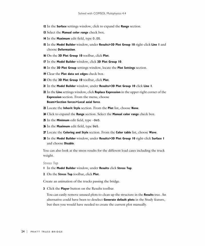
Solved with COMSOL Multiphysics 4.4
24 | P R
12 In the Surface settings window, click to expand the Range section.
13 Select the Manual color range check box.
14 In the Maximum edit field, type 0.05.
15 In the Model Builder window, under Results>3D Plot Group 10 right-click Line 1 and choose Deformation.
16 On the 3D Plot Group 10 toolbar, click Plot.
17 In the Model Builder window, click 3D Plot Group 10.
18 In the 3D Plot Group settings window, locate the Plot Settings section.
19 Clear the Plot data set edges check box.
20 On the 3D Plot Group 10 toolbar, click Plot.
21 In the Model Builder window, under Results>3D Plot Group 10 click Line 1.
22 In the Line settings window, click Replace Expression in the upper-right corner of the Expression section. From the menu, choose Beam>Section forces>Local axial force.
23 Locate the Inherit Style section. From the Plot list, choose None.
24 Click to expand the Range section. Select the Manual color range check box.
25 In the Minimum edit field, type -9e5.
26 In the Maximum edit field, type 9e5.
27 Locate the Coloring and Style section. From the Color table list, choose Wave.
28 In the Model Builder window, under Results>3D Plot Group 10 right-click Surface 1 and choose Disable.
You can also look at the stress results for the different load cases including the truck weight.
Stress Top1 In the Model Builder window, under Results click Stress Top.
2 On the Stress Top toolbar, click Plot.
Create an animation of the trucks passing the bridge.
3 Click the Player button on the Results toolbar.
You can easily remove unused plots to clean up the structure in the Results tree. An alternative could have been to deselect Generate default plots in the Study feature, but then you would have needed to create the current plot manually.
A T T TR U S S B R I D G E

Solved with COMSOL Multiphysics 4.4
4 In the Model Builder window, select Results>Stress Bottom 1, hold down the Shift key, and then select Results>Torsion Moment 1. Right click and choose Delete.
R O O T
On the Home toolbar, click Add Study.
A D D S T U D Y
1 Go to the Add Study window.
2 Find the Studies subsection. In the tree, select Preset Studies>Eigenfrequency.
3 In the Add study window, click Add Study.
4 On the Home toolbar, click Add Study.
S T U D Y 2
Step 1: Eigenfrequency1 In the Model Builder window, under Study 2 click Step 1: Eigenfrequency.
2 In the Eigenfrequency settings window, locate the Study Settings section.
3 In the Desired number of eigenfrequencies edit field, type 12.
4 On the Home toolbar, click Compute.
R E S U L T S
Mode ShapeSelect the first mode involving the roadway.
1 In the Model Builder window, click Mode Shape.
2 In the 3D Plot Group settings window, locate the Data section.
3 From the Eigenfrequency list, choose 3.326944.
4 In the Model Builder window, expand the Mode Shape node.
Mode Shape1 In the Model Builder window, expand the Results>Mode Shape node.
2 Right-click Line 1 and choose Copy.
Mode Shape1 In the Model Builder window, under Results right-click Mode Shape and choose Paste
Line.
2 In the Line settings window, locate the Inherit Style section.
25 | P R A T T TR U S S B R I D G E

Solved with COMSOL Multiphysics 4.4
26 | P R
3 From the Plot list, choose Surface 1.
4 In the Model Builder window, expand the Results>Mode Shape>Surface 1 node, then click Deformation.
5 In the Deformation settings window, locate the Scale section.
6 Select the Scale factor check box.
7 In the associated edit field, type 0.2.
8 In the Model Builder window, under Results>Mode Shape click Surface 1.
9 In the Surface settings window, locate the Range section.
10 Select the Manual color range check box.
11 In the Maximum edit field, type 4.
12 On the Mode Shape toolbar, click Plot.
A T T TR U S S B R I D G E

Solved with COMSOL Multiphysics 4.4
S ubmode l i n a Whee l R im
Introduction
In stress analysis, it is common that the regions with high stresses are small when compared to the whole structure. Sometimes it is not feasible to have a mesh that at the same time captures the global behavior and resolves the stress concentrations with high accuracy. This is especially true in nonlinear or dynamic problems.
You can cope with this type of problems with a technique known as submodeling. First you solve the complete model with a mesh which is sufficient to capture the stiffness of the structure. In a second analysis you create a local model (submodel) of the region around the stress concentration with a fine mesh, and solve it using the displacements from the global model as boundary conditions.
There are a some underlying assumptions when using submodels:
• The global model is accurate enough to give correct displacements on the boundary to the submodel.
• The improvements introduced in the submodel are so small that they do not introduce significant changes in stiffness on the global level. Given this, it could still be possible to introduce a nonlinear material locally in the submodel.
This example shows how to perform submodel analysis in COMSOL Multiphysics.
Model Definition
The wheel rim for this analysis is a ten-spoke example where the design elements of the geometry cause the finite element mesh to become quite large. The loading on the tire is composed of both the tire pressure and a load transferred from the road via the tire to the rim. In this case you study only one loadcase which is symmetric with respect to the geometry, so it is sufficient to use one half of the geometry as shown in Figure 1.
In the submodel (shown in Figure 3), you cut out a small region around the hot spot using an intersection between the rim geometry and a 70 mm-by-70 mm-by-60 mm block.
M A T E R I A L
Aluminum with E = 70 GPa, = 0.33.
1 | S U B M O D E L I N A W H E E L R I M

Solved with COMSOL Multiphysics 4.4
2 | S U B
C O N S T R A I N T S
• A region around each bolt hole is fixed.
• Symmetry condition (normal displacement fixed) in the symmetry plane.
Figure 1: The boundary conditions.
L O A D S
• Tire pressure: The overpressure is 2 bar = 200 kPa.
• The total load carried by the wheel corresponds to a weight of 1120 kg. It is applied as a pressure on the rim surfaces where the tire is in contact. Assume that the load distribution in the circumferential direction can be approximated as pp0 cos 3 ,
Symmetric boundary condition
Fixed boundary condition
M O D E L I N A W H E E L R I M

Solved with COMSOL Multiphysics 4.4
where is the angle from the point of contact between the road and the tire. The loaded area thus extends 30 in each direction.
Figure 2: The applied loads: a tire pressure and the load from the road.
Load from road
Tire pressure
3 | S U B M O D E L I N A W H E E L R I M

Solved with COMSOL Multiphysics 4.4
4 | S U B
Figure 3: The submodel geometry.
Results and Discussion
The highest stresses occur in the fillet where the spoke connects to the hub. In the global model the maximum effective stress is completely mesh dependent, and not reliable. In the submodel, where the resolution is good, the effective stress is 94.7 MPa. In a fatigue analysis where the lifetime could vary as the fifth power of the stress it is essential to get this level of accuracy in the critical regions.
There are some stress disturbances at the boundaries where the displacements from the global model are applied. This is a result of the fact that in the coarse model, the meshed representation of the geometry is not good enough, so displacement boundary conditions for the submodel has to be extrapolated outside of the global mesh.
Cut surfaces with displacements mapped from global model
M O D E L I N A W H E E L R I M
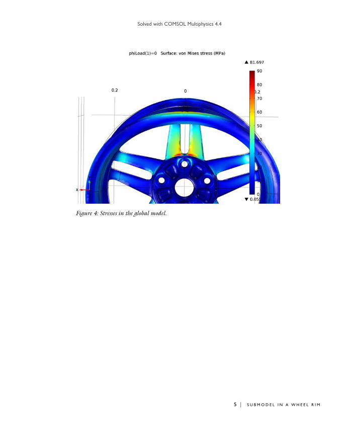
Solved with COMSOL Multiphysics 4.4
Figure 4: Stresses in the global model.
5 | S U B M O D E L I N A W H E E L R I M

Solved with COMSOL Multiphysics 4.4
6 | S U B
Figure 5: Stresses in the submodel.
Notes About the COMSOL Implementation
Two different models are used within the same mph file. In the global model, a general extrusion feature is introduced in order to describe the mapping of results from the global model to the submodel.
Model Library path: Structural_Mechanics_Module/Tutorial_Models/rim_submodel
Modeling Instructions
From the File menu, choose New.
N E W
1 In the New window, click the Model Wizard button.
M O D E L I N A W H E E L R I M

Solved with COMSOL Multiphysics 4.4
M O D E L W I Z A R D
1 In the Model Wizard window, click the 3D button.
2 In the Select Physics tree, select Structural Mechanics>Solid Mechanics (solid).
3 Click the Add button.
4 Click the Study button.
5 In the Select Study tree, select Preset Studies>Stationary.
6 Click the Done button.
G L O B A L D E F I N I T I O N S
Parameters1 On the Home toolbar, click Parameters.
2 In the Parameters settings window, locate the Parameters section.
3 In the table, enter the following settings:
G E O M E T R Y 1
Import 11 On the Home toolbar, click Import.
2 In the Import settings window, locate the Import section.
3 Click the Browse button.
4 Browse to the model’s Model Library folder and double-click the file wheel_rim.mphbin.
Name Expression Value Description
pInflation 2[bar] 2.000E5 Pa Inflation pressure
tireLoad 1120[kg]*g_const 1.098E4 N Load on wheel
spokeNo 0 0 Spoke selection
spokeAngle spokeNo*2*pi[rad]/5 0 rad Rotation angle to selected spoke
phiLoad 0 0 Peak load angle
numLpos 4 4.000 Number of load positions in first sector
angleStep 360/(5*numLpos) 18.00 Step in peak load angle [deg]
angleLast angleStep*(numLpos-1) 54.00 Last peak load angle [deg]
7 | S U B M O D E L I N A W H E E L R I M

Solved with COMSOL Multiphysics 4.4
8 | S U B
5 Click the Import button.
Form UnionIn the Model Builder window, under Component 1>Geometry 1 right-click Form Union and choose Build Selected.
D E F I N I T I O N S
Explicit 11 On the Definitions toolbar, click Explicit.
2 In the Explicit settings window, locate the Input Entities section.
3 From the Geometric entity level list, choose Boundary.
4 Select Boundaries 9–12, 22, 23, 26, 27, 460, 461, 464, 466, and 541–544 only.
5 Right-click Component 1>Definitions>Explicit 1 and choose Rename.
6 Go to the Rename Explicit dialog box and type TireAttachment in the New name edit field.
7 Click OK.
Explicit 21 On the Definitions toolbar, click Explicit.
2 In the Explicit settings window, locate the Input Entities section.
3 From the Geometric entity level list, choose Boundary.
4 Select Boundaries 9–12, 22–29, 38–41, 48–51, 64, 65, 460, 461, 464–469, 472, 473, 476, 531–533, 536, 537, and 539–544 only.
5 Right-click Component 1>Definitions>Explicit 2 and choose Rename.
6 Go to the Rename Explicit dialog box and type PressureSurface in the New name edit field.
7 Click OK.
Explicit 31 On the Definitions toolbar, click Explicit.
2 In the Explicit settings window, locate the Input Entities section.
3 From the Geometric entity level list, choose Boundary.
4 Select Boundaries 236, 287, 434, 508, 606, and 682 only.
5 Right-click Component 1>Definitions>Explicit 3 and choose Rename.
M O D E L I N A W H E E L R I M

Solved with COMSOL Multiphysics 4.4
6 Go to the Rename Explicit dialog box and type FixedToHub in the New name edit field.
7 Click OK.
M A T E R I A L S
On the Home toolbar, click More Windows and choose Add Material.
A D D M A T E R I A L
1 Go to the Add Material window.
2 In the tree, select Built-In>Aluminum.
3 In the Add Material window, click Add to Component.
M A T E R I A L S
AluminumIn the Model Builder window’s toolbar, click the Show button and select Advanced
Physics Options in the menu.
S O L I D M E C H A N I C S
Fixed Constraint 11 On the Physics toolbar, click Boundaries and choose Fixed Constraint.
2 In the Fixed Constraint settings window, locate the Boundary Selection section.
3 From the Selection list, choose FixedToHub.
Boundary Load 11 On the Physics toolbar, click Boundaries and choose Boundary Load.
2 In the Boundary Load settings window, locate the Boundary Selection section.
3 From the Selection list, choose PressureSurface.
4 Locate the Force section. From the Load type list, choose Pressure.
5 In the p edit field, type pInflation.
D E F I N I T I O N S
Analytic 11 On the Home toolbar, click Functions and choose Global>Analytic.
2 In the Analytic settings window, locate the Definition section.
9 | S U B M O D E L I N A W H E E L R I M

Solved with COMSOL Multiphysics 4.4
10 | S U
3 In the Expression edit field, type (abs(atan2(x,y)-z*pi/180)<pi/6)*cos(3*(atan2(x,y)-z*pi/180)).
4 In the Arguments edit field, type x, y, z.
5 Locate the Units section. In the Arguments edit field, type m,m,1.
6 In the Function edit field, type Pa.
7 Locate the Function Name section. In the Function name edit field, type loadDistr.
8 On the Definitions toolbar, click Coordinate Systems and choose Cylindrical System.
S O L I D M E C H A N I C S
Boundary Load 21 On the Physics toolbar, click Boundaries and choose Boundary Load.
2 In the Boundary Load settings window, locate the Coordinate System Selection section.
3 From the Coordinate system list, choose Cylindrical System 2.
4 Locate the Boundary Selection section. From the Selection list, choose TireAttachment.
5 Locate the Force section. Specify the FA vector as
D E F I N I T I O N S
Integration 11 On the Definitions toolbar, click Component Couplings and choose Integration.
2 In the Integration settings window, locate the Source Selection section.
3 From the Geometric entity level list, choose Boundary.
4 From the Selection list, choose TireAttachment.
S O L I D M E C H A N I C S
Global Equations 11 On the Physics toolbar, click Global and choose Global Equations.
2 In the Global Equations settings window, locate the Global Equations section.
-loadAmpl*loadDistr(X,Y,phiLoad) r
0 phi
0.2*loadAmpl*loadDistr(X,Y,phiLoad)*(2*(Z>0)-1) a
B M O D E L I N A W H E E L R I M

Solved with COMSOL Multiphysics 4.4
3 In the table, enter the following settings:
M E S H 1
In the Model Builder window, under Component 1 right-click Mesh 1 and choose Free Tetrahedral.
Size1 In the Model Builder window, under Component 1>Mesh 1 click Size.
2 In the Size settings window, locate the Element Size section.
3 Click the Custom button.
4 Locate the Element Size Parameters section. In the Maximum element size edit field, type 0.04.
5 In the Minimum element size edit field, type 0.007.
6 In the Resolution of narrow regions edit field, type 0.4.
7 Click the Build All button.
S T U D Y 1
Step 1: Stationary1 In the Model Builder window, under Study 1 click Step 1: Stationary.
2 In the Stationary settings window, click to expand the Study Extensions section.
3 Locate the Study Extensions section. Select the Auxiliary sweep check box.
4 Click Add.
5 In the table, enter the following settings:
Name f(u,ut,utt,t) (1) Initial value (u_0) (1)
Initial value (u_t0) (1/s)
Description
loadAmpl loadAmpl*intop1(loadDistr(X,Y,0)*cos(atan2(X,Y)))-tireLoad
0 0
Auxiliary parameter Parameter value list
phiLoad range(0,angleStep,angleLast)
11 | S U B M O D E L I N A W H E E L R I M

Solved with COMSOL Multiphysics 4.4
12 | S U
Solver 11 On the Study toolbar, click Show Default Solver.
Because of the model's considerable size, you set up an iterative solver that can significantly save on the memory needed for the computations. Use the GMRES iterative solver with Geometric Multigrid as a preconditioner. By default, the solver lowers the order in the discretization of the displacement variables from the default quadratic elements to linear elements. Because the model geometry contains slender elements, use SOR Line as presmoother and postsmoother. SOR Line can handle slender geometries better than the SOR presmoother used by default. Note however that it cannot make full use of the matrix symmetry.
2 In the Model Builder window, expand the Solver 1 node.
3 Right-click Stationary Solver 1 and choose Iterative.
4 Right-click Study 1>Solver Configurations>Solver 1>Stationary Solver 1>Iterative 1 and choose Multigrid.
5 In the Model Builder window, expand the Study 1>Solver Configurations>Solver
1>Stationary Solver 1>Iterative 1>Multigrid 1 node.
6 Right-click Presmoother and choose SOR Line.
7 Right-click Study 1>Solver Configurations>Solver 1>Stationary Solver 1>Iterative
1>Multigrid 1>Postsmoother and choose SOR Line.
8 On the Home toolbar, click Compute.
R E S U L T S
Stress (solid)1 In the Model Builder window, click Stress (solid).
2 In the 3D Plot Group settings window, locate the Data section.
3 From the Parameter value (phiLoad) list, choose 0.
4 In the Model Builder window, under Results>Stress (solid) click Surface 1.
5 In the Surface settings window, locate the Expression section.
6 From the Unit list, choose MPa.
7 Click to expand the Range section. Select the Manual color range check box.
8 In the Minimum edit field, type 0.
9 In the Maximum edit field, type 90.
To get a better view of the region with the highest stresses (compare with Figure 4), rotate the geometry in the Graphics window and use the Zoom Box tool to obtain
B M O D E L I N A W H E E L R I M

Solved with COMSOL Multiphysics 4.4
a close-up. You can preserve a view for a plot by creating a View feature node as follows:
10 In the Model Builder window’s toolbar, click the Show button and select Advanced
Results Options in the menu.
11 In the Model Builder window, under Results right-click Views and choose View 3D.
In the graphics window rotate the model and capture the part with largest stresses.
View 3D 21 In the Model Builder window, under Results>Views click View 3D 2.
2 In the View 3D settings window, locate the View section.
3 Select the Lock camera check box.
Stress (solid)1 In the Model Builder window, under Results click Stress (solid).
2 In the 3D Plot Group settings window, locate the Plot Settings section.
3 From the View list, choose View 3D 2.
4 In the Model Builder window, click Stress (solid).
5 On the Stress (solid) toolbar, click Plot.
Start creating the submodel.
R O O T
On the Home toolbar, click Add Component and choose 3D.
G E O M E T R Y 2
1 On the Home toolbar, click More Windows and choose Add Physics.
A D D P H Y S I C S
1 Go to the Add Physics window.
2 In the Add physics tree, select Structural Mechanics>Solid Mechanics (solid).
3 Find the Physics in study subsection. In the table, enter the following settings:
4 In the Add Physics window, click Add to Component.
Studies Solve
Study 1 ×
13 | S U B M O D E L I N A W H E E L R I M

Solved with COMSOL Multiphysics 4.4
14 | S U
R O O T
1 On the Home toolbar, click More Windows and choose Add Study.
A D D S T U D Y
1 Go to the Add Study window.
2 Find the Studies subsection. In the tree, select Preset Studies>Stationary.
3 Find the Physics in study subsection. In the table, enter the following settings:
4 In the Add Study window, click Add Study.
S T U D Y 2
G E O M E T R Y 2
Import 11 On the Home toolbar, click Import.
2 In the Import settings window, locate the Import section.
3 Click the Browse button.
4 Browse to the model’s Model Library folder and double-click the file wheel_rim.mphbin.
5 Click the Import button.
6 Click the Build All Objects button.
Block 11 On the Geometry toolbar, click Block.
2 In the Block settings window, locate the Position section.
3 In the y edit field, type 0.065.
4 In the z edit field, type 0.06.
5 Locate the Size section. In the Width edit field, type 0.06.
6 In the Depth edit field, type 0.07.
7 In the Height edit field, type 0.06.
8 Click the Build All Objects button.
Physics Solve
Solid Mechanics (solid) ×
B M O D E L I N A W H E E L R I M

Solved with COMSOL Multiphysics 4.4
Intersection 11 On the Geometry toolbar, click Intersection.
2 Select the objects blk1 and imp1 only.
3 Click the Build All Objects button.
Form UnionOn the Home toolbar, click Build All.
Form Composite Faces 11 On the Geometry toolbar, click Virtual Operations and choose Form Composite Faces.
2 On the object fin, select Boundaries 9, 15, 16, 18–21, 30, 33, 42, 44, 46, and 48 only.
3 On the Home toolbar, click Build All.
Form Composite Faces 21 On the Geometry toolbar, click Virtual Operations and choose Form Composite Faces.
2 On the object cmf1, select Boundaries 10, 16, 18, and 19 only.
3 On the Home toolbar, click Build All.
4 Click the Zoom Extents button on the Graphics toolbar.
A D D M A T E R I A L
1 Go to the Add Material window.
2 In the tree, select Built-In>Aluminum.
3 In the Add Material window, click Add to Component.
D E F I N I T I O N S
General Extrusion 11 On the Definitions toolbar, click Component Couplings and choose General Extrusion.
2 In the General Extrusion settings window, locate the Source Selection section.
3 From the Selection list, choose All domains.
4 Locate the Source section. From the Source frame list, choose Material (X, Y, Z).
5 Locate the Destination Map section. In the x-expression edit field, type X*cos(spokeAngle)-Y*sin(spokeAngle).
6 In the y-expression edit field, type Y*cos(spokeAngle)+X*sin(spokeAngle).
7 In the z-expression edit field, type Z.
15 | S U B M O D E L I N A W H E E L R I M

Solved with COMSOL Multiphysics 4.4
16 | S U
8 Locate the Operator Name section. In the Operator name edit field, type from_global.
S O L I D M E C H A N I C S 2
Fixed Constraint 11 On the Physics toolbar, click Boundaries and choose Fixed Constraint.
2 Select Boundary 5 only.
Prescribed Displacement 11 On the Physics toolbar, click Boundaries and choose Prescribed Displacement.
2 Select Boundaries 1, 18, 25, and 43 only.
3 In the Prescribed Displacement settings window, locate the Prescribed Displacement section.
4 Select the Prescribed in x direction check box.
5 In the u0x edit field, type comp1.from_global(comp1.u*cos(spokeAngle)+comp1.v*sin(spokeAngle)
).
6 Select the Prescribed in y direction check box.
7 In the u0y edit field, type comp1.from_global(comp1.v*cos(spokeAngle)-comp1.u*sin(spokeAngle)
).
8 Select the Prescribed in z direction check box.
9 In the u0z edit field, type comp1.from_global(comp1.w).
M E S H 2
1 In the Model Builder window, under Component 2 click Mesh 2.
2 In the Mesh settings window, locate the Mesh Settings section.
3 From the Element size list, choose Fine.
4 From the Sequence type list, choose User-controlled mesh.
Size 11 In the Model Builder window, under Component 2>Mesh 2 right-click Free Tetrahedral
1 and choose Size.
2 In the Size settings window, locate the Geometric Entity Selection section.
3 From the Geometric entity level list, choose Boundary.
B M O D E L I N A W H E E L R I M

Solved with COMSOL Multiphysics 4.4
4 Select Boundary 14 only.
5 Locate the Element Size section. From the Predefined list, choose Extremely fine.
6 Click the Build All button.
S T U D Y 2
Step 1: Stationary1 In the Model Builder window, expand the Study 2 node, then click Step 1: Stationary.
2 In the Stationary settings window, click to expand the Values of Dependent Variables section.
Fetch the displacements from the solution of the global model.
3 Locate the Values of Dependent Variables section. Select the Values of variables not
solved for check box.
4 From the Method list, choose Solution.
5 From the Study list, choose Study 1, Stationary.
6 From the Parameter value (phiLoad) list, choose All.
7 Locate the Study Extensions section. Select the Auxiliary sweep check box.
8 From the Sweep type list, choose All combinations.
9 Click Add.
10 In the table, enter the following settings:
11 Click Add.
12 In the table, add the following settings:
Solver 21 On the Study toolbar, click Show Default Solver.
For the submodel, you also use an iterative solver with GMG as preconditioner. You select the Conjugate gradients solver because it can make full use of the matrix symmetry, thus saving memory.
Auxiliary parameter Parameter value list
spokeNo range(0,1,4)
Auxiliary parameter Parameter value list
phiLoad range(0,angleStep,angleLast)
17 | S U B M O D E L I N A W H E E L R I M

Solved with COMSOL Multiphysics 4.4
18 | S U
2 In the Model Builder window, expand the Study 2>Solver Configurations>Solver
2>Stationary Solver 1 node.
3 Right-click Study 2>Solver Configurations>Solver 2>Stationary Solver 1 and choose Iterative.
4 In the Iterative settings window, locate the General section.
5 From the Solver list, choose Conjugate gradients.
6 Right-click Study 2>Solver Configurations>Solver 2>Stationary Solver 1>Iterative 1 and choose Multigrid.
7 In the Multigrid settings window, locate the General section.
8 In the Use hierarchy in geometries list, select Geometry 1.
9 Under Use hierarchy in geometries, click Delete.
S T U D Y 1
Solver 11 In the Model Builder window, under Study 1>Solver Configurations>Solver
1>Stationary Solver 1>Iterative 1 click Multigrid 1.
2 In the Multigrid settings window, locate the General section.
3 In the Use hierarchy in geometries list, select Geometry 1.
4 Under Use hierarchy in geometries, click Delete.
Avoid saving a lot of duplicate results for the full geometry.
S T U D Y 2
Solver 21 In the Model Builder window, expand the Study 2>Solver Configurations>Solver
2>Dependent Variables 1 node, then click Displacement field (Material) (comp1.u).
2 In the Field settings window, locate the General section.
3 Clear the Store in output check box.
4 In the Model Builder window, under Study 2>Solver Configurations>Solver
2>Dependent Variables 1 click State variable loadAmpl (comp1.ODE1).
5 In the State settings window, locate the General section.
6 Clear the Store in output check box.
7 On the Home toolbar, click Compute.
B M O D E L I N A W H E E L R I M

Solved with COMSOL Multiphysics 4.4
R E S U L T S
Stress (solid2)1 In the Model Builder window, expand the Stress (solid2) node, then click Surface 1.
2 In the Surface settings window, locate the Expression section.
3 From the Unit list, choose MPa.
4 Locate the Range section. Select the Manual color range check box.
5 In the Minimum edit field, type 0.
6 In the Maximum edit field, type 90.
7 In the Model Builder window, click Stress (solid2).
8 In the 3D Plot Group settings window, locate the Data section.
9 From the Parameter value (spokeNo) list, choose 0.
10 From the Parameter value (phiLoad) list, choose 18.
11 On the Stress (solid2) toolbar, click More Plots and choose More Plots>Principal Stress
Surface.
12 In the Model Builder window, under Results>Stress (solid2) right-click Principal Stress
Surface 1 and choose Deformation.
13 In the Model Builder window, under Results>Stress (solid2) click Principal Stress
Surface 1.
14 In the Principal Stress Surface settings window, click to expand the Inherit Style section.
15 Locate the Inherit Style section. From the Plot list, choose Surface 1.
16 Clear the Arrow scale factor check box.
17 Clear the Color check box.
18 Clear the Color and data range check box.
19 In the Model Builder window, right-click Stress (solid2) and choose Rename.
20 Go to the Rename 3D Plot Group dialog box and type Stress in Submodel in the New name edit field.
21 Click OK.
Again, create a View 3D feature node for the plot
View 3D 41 Right-click Results>Views and choose View 3D.
2 In the View 3D settings window, locate the View section.
19 | S U B M O D E L I N A W H E E L R I M

Solved with COMSOL Multiphysics 4.4
20 | S U
3 Clear the Show grid check box.
In the graphics window rotate the model and capture the part with largest stresses.
View 3D 41 In the Model Builder window, under Results>Views click View 3D 4.
2 In the View 3D settings window, locate the View section.
3 Select the Lock camera check box.
Apply the view to 3D Plot Group 3.
Stress in Submodel1 In the Model Builder window, under Results click Stress in Submodel.
2 In the 3D Plot Group settings window, locate the Plot Settings section.
3 From the View list, choose View 3D 4.
4 On the Stress in Submodel toolbar, click Plot.
Finally, create an animation, showing the stress history for a complete revolution of the wheel.
Export1 On the Results toolbar, click Player.
2 In the Player settings window, locate the Scene section.
3 From the Subject list, choose Stress in Submodel.
4 Locate the Animation Editing section. From the Loop over list, choose All solutions.
5 In the Parameter values (phiLoad,spokeNo) list, choose all values.
6 Locate the Frames section. From the Frame selection list, choose All.
7 Click the Generate Frame button.
8 Right-click Results>Export>Player 1 and choose Play.
B M O D E L I N A W H E E L R I M

Solved with COMSOL Multiphysics 4.4
E i g e n f r e qu en c y Ana l y s i s o f a Ro t a t i n g B l a d e
Introduction
High rotational speed in, for example, gas turbine machinery can result in centrifugal forces of considerable magnitude. This model studies the effects of such forces on the natural frequencies of the structure.
The fictitious forces induced by the rotation give rise to two counteracting effects: stress-stiffening and spin-softening (or centrifugal softening). The former is caused by the stationary stress field created by the centrifugal force and acts to increase the stiffness of the body, and so increase its resonance frequencies. At the same time, any radial displacement away from the axis of rotation increases the centrifugal force, while motion toward the axis decreases it. This effect therefore tends to amplify any radial motion, which is the opposite of stiffening—hence spin-softening. Which mechanism is dominating depends on the shape of the particular mode.
In some rotating systems, Coriolis forces can also play an important role. These apparent forces split some natural modes of vibration into one co-rotating and one counter-rotating precessing mode. In particular, this happens for natural modes that include bending of the axis of rotation. For most modes of vibration, however, the Coriolis frequency shifts are small.
Model Definition
In the first part of the model you conduct a modal analysis of a blade mounted on a rigid rotating cylinder. The rotational speed is 3000 rpm (100 rad/s) about the global y-axis. The goal is to compare the fundamental frequency in three cases:
• A basic modal analysis at 0 rpm, thus excluding any fictitious force effects.
• A modal analysis including stress-stiffening and spin-softening at 3000 rpm.
• A complete analysis also including Coriolis effects at 3000 rpm.
The result in the first two cases can be compared directly to an analytical reference solution. Once you are satisfied that the solutions are accurate in all cases, the second step proceeds to compute the first few natural frequencies for a large range of rotational speeds.
1 | E I G E N F R E Q U E N C Y A N A L Y S I S O F A R O T A T I N G B L A D E

Solved with COMSOL Multiphysics 4.4
2 | E I G
F I C T I T I O U S F O R C E S I N R O T A T I N G C O O R D I N A T E S Y S T E M S
The spin-softening and Coriolis effects both ultimately arise because the standard form of the laws governing the deformation of solid objects only hold in inertial, that is, nonaccelerating, coordinate systems. When you build and simulate a model in a rotating coordinate system, you must extend the basic laws of motion to account for the acceleration of the system itself.
In COMSOL Multiphysics, you can model the frame acceleration effects by using the Rotating Frame domain feature.
In this particular case, the axis of rotation is the y-axis, see Figure 1. The only explicit boundary condition in the model is on the blade’s base, which is fixed to the axis.
S T R E S S - S T I F F E N I N G A N D N O N L I N E A R E F F E C T S
To include the stress-stiffening effects in the model, you activate the large deformation option. This redefines the strain measure to include second-order terms, which make the strain-displacement relation nonlinear. The resulting strain measure is called Green strain.
For the stress stiffening to have any effect on the natural frequencies, you must first solve for the stationary stresses from the centrifugal loading in a stationary analysis. Then you perform the modal analysis using the static solution as a linearization point.
Note that the spin-softening affects not only the modal solution but also adds a positive feedback to the stationary nonlinear solution. If the structure has a natural mode for which spin-softening dominates over the stress-stiffening effect, the natural frequency of this mode becomes zero for some rotational frequency. This means that the structure looses all stiffness, and that no stable solution exists for higher angular velocities. So if the nonlinear solver does not converge for a very fast rotation, it should come as no surprise.
M A T E R I A L A N D G E O M E T R I C A L P R O P E R T I E S
The blade’s material and geometrical properties are given in the table below (see also Figure 1):
MATERIAL PROPERTIES GEOMETRIC PROPERTIES
E 221·109 Pa Young’s modulus r 10 in Cylinder radius
0 Poisson’s ratio L 5 in Blade length
7850 kg/m3 Density d 0.0625 in Blade thickness
b 1 in Blade width
E N F R E Q U E N C Y A N A L Y S I S O F A R O T A T I N G B L A D E

Solved with COMSOL Multiphysics 4.4
The approximate equation for the natural frequency in Ref. 1 does not include the Poisson’s ratio. To facilitate easy comparison with the COMSOL Multiphysics model, the Poisson’s ratio is set to zero in the model as well.
Figure 1: Blade geometry.
A N A L Y T I C A L S O L U T I O N S
You can compare COMSOL Multiphysics’ results to an accurate analytical approximation. Using Euler beam theory, which is sufficiently accurate for the present geometry, the fundamental angular frequency for the nonrotating case is given by
where E is the Young’s modulus, I is the area moment of inertia, m is the mass per unit length, and L is the blade length.
For a rotating blade attached to a rigid axis with radius r and rotating with angular frequency , the fundamental angular frequency according to Ref. 1 is
w0 1.8752 EI
mL4------------=
3 | E I G E N F R E Q U E N C Y A N A L Y S I S O F A R O T A T I N G B L A D E

Solved with COMSOL Multiphysics 4.4
4 | E I G
This formula assumes a blade of uniform cross section slanted at the so-called stagger angle . In the present case, . The author states without proof that the Coriolis effect is negligible. You can check the validity of this statement by comparing the finite element solutions with and without the Coriolis term included.
Results and Discussion
The following table shows a comparison between the analytical results and the results computed in COMSOL Multiphysics:
Apparently, the Coriolis effect is negligible as stated in Ref. 1. Because including the Coriolis terms makes the system of equations nonsymmetric—and therefore more
CASE ANALYTICAL RESULT COMSOL RESULTS
0 rpm 84.4 Hz 84.4 Hz
3000 rpm, no Coriolis effect 123.6 Hz 124 Hz
3000 rpm, with Coriolis effect - 124 Hz
w w0 1 m2r4 EI
-----------------------+18--- L
r---- 3 1
10.6----------- L
r---- 4
+cos 2
12.45-------------------- L
r---- 4
–=
0=
E N F R E Q U E N C Y A N A L Y S I S O F A R O T A T I N G B L A D E

Solved with COMSOL Multiphysics 4.4
expensive to solve—there is, in general, no need to include the Coriolis effect when modeling systems with a rigid axis.
Figure 2: Campbell diagram created from the parametric sweep output file. Notice the crossing modes, which are misinterpreted because of the sorting of the natural frequencies.
The Campbell diagram, see Figure 2, shows that the first 6 natural frequencies all increase with increasing rotational speed. However, the balance between stress stiffening and spin softening is different for the different modes. Stress stiffening is more pronounced for modes 2 and 5 (referring to the mode order at zero rotational frequency) compared to the others. Therefore, the order of the modes in the result file—which is sorted on mode frequency—changes with increasing rotational velocity.
Notes About the COMSOL Implementation
Note that the eigenvalue solver always finds the requested number of modes but not necessarily the ones with lowest eigenfrequencies. Sometimes it can converge on a higher-order mode instead. A jagged appearance of the highest frequency mode in the Campbell diagram is a result of the solver’s picking a higher mode instead of requested highest mode for some rotational frequencies. In order to avoid this behavior it is recommended to solve for one additional eigenfrequency in the study and display results for all eigenfrequencies except the one of the highest mode.
5 | E I G E N F R E Q U E N C Y A N A L Y S I S O F A R O T A T I N G B L A D E

Solved with COMSOL Multiphysics 4.4
6 | E I G
When eigenfrequencies are calculated, numerical noise can occasionally be seen via the imaginary part of the eigenfrequency. If the imaginary part is several orders of magnitude smaller than the real part then use the real part as the eigenfrequency and disregard the imaginary part.
Reference
1. W. Carnegie, “Vibrations of Rotating Cantilever Blading,” J. Mech. Engrg Sci., vol. 1, no. 3, London, 1959.
Model Library path: Structural_Mechanics_Module/Dynamics_and_Vibration/rotating_blade
Modeling Instructions
From the File menu, choose New.
N E W
1 In the New window, click the Model Wizard button.
M O D E L W I Z A R D
1 In the Model Wizard window, click the 3D button.
2 In the Select physics tree, select Structural Mechanics>Solid Mechanics (solid).
3 Click the Add button.
4 Click the Study button.
5 In the tree, select Preset Studies>Prestressed Analysis, Eigenfrequency.
6 Click the Done button.
G L O B A L D E F I N I T I O N S
Parameters1 On the Home toolbar, click Parameters.
2 In the Parameters settings window, locate the Parameters section.
E N F R E Q U E N C Y A N A L Y S I S O F A R O T A T I N G B L A D E

Solved with COMSOL Multiphysics 4.4
3 In the table, enter the following settings:
G E O M E T R Y 1
Block 11 On the Geometry toolbar, click Block.
2 In the Block settings window, locate the Size section.
3 In the Width edit field, type L.
4 In the Depth edit field, type b.
5 In the Height edit field, type d.
6 Locate the Position section. In the x edit field, type r.
7 In the z edit field, type -d/2.
8 Click the Build Selected button.
Name Expression Value Description
Omega 0*pi[rad/s] 0 rad/s Angular velocity
L 5[in] 0.1270 m Blade length
b 1[in] 0.02540 m Blade width
d 0.0625[in] 0.001588 m Blade thickness
E0 221[GPa] 2.210E11 Pa Young's modulus
rho0 7850[kg/m^3] 7850 kg/m³ Density
r 10[in] 0.2540 m Inner radius
mpl rho0*b*d 0.3165 kg/m Mass per unit length
I b*d^3/12 8.468E-12 m4 Area moment of inertia
f_0 1.875^2*sqrt(E0*I/(mpl*L^4))/(2*pi)
84.35 1/s Euler beam resonance frequency
f_ref f_0*sqrt(1+mpl*Omega^2*r^4/(E0*I)*((L/r)^3/8+(L/r)^4*(1/10.6-1/12.45)))
84.35 rad/s Reference resonance frequency
7 | E I G E N F R E Q U E N C Y A N A L Y S I S O F A R O T A T I N G B L A D E

Solved with COMSOL Multiphysics 4.4
8 | E I G
Form UnionIn the Model Builder window, under Component 1>Geometry 1 right-click Form Union and choose Build Selected.
M A T E R I A L S
Material 11 In the Model Builder window, under Component 1 right-click Materials and choose
New Material.
2 Select Domain 1 only.
3 In the Material settings window, locate the Material Contents section.
4 In the table, enter the following settings:
S O L I D M E C H A N I C S
Rotating Frame 11 On the Physics toolbar, click Domains and choose Rotating Frame.
2 Select Domain 1 only.
3 In the Rotating Frame settings window, locate the Rotating Frame section.
4 From the Axis of rotation list, choose y-axis.
5 In the edit field, type Omega.
Fixed Constraint 11 On the Physics toolbar, click Boundaries and choose Fixed Constraint.
2 Select Boundary 1 only.
M E S H 1
Mapped 11 In the Model Builder window, under Component 1 right-click Mesh 1 and choose
Mapped.
2 Select Boundary 4 only.
Property Name Value Unit Property group
Young's modulus E E0 Pa Basic
Poisson's ratio nu 0 1 Basic
Density rho rho0 kg/m³ Basic
E N F R E Q U E N C Y A N A L Y S I S O F A R O T A T I N G B L A D E

Solved with COMSOL Multiphysics 4.4
Distribution 11 Right-click Component 1>Mesh 1>Mapped 1 and choose Distribution.
2 Select Edge 4 only.
Distribution 21 Right-click Mapped 1 and choose Distribution.
2 Select Edge 5 only.
3 In the Distribution settings window, locate the Distribution section.
4 In the Number of elements edit field, type 25.
Mapped 1Right-click Mapped 1 and choose Build Selected.
Swept 1Right-click Mesh 1 and choose Swept.
Distribution 11 In the Model Builder window, under Component 1>Mesh 1 right-click Swept 1 and
choose Distribution.
2 Select Domain 1 only.
3 In the Distribution settings window, locate the Distribution section.
4 In the Number of elements edit field, type 4.
9 | E I G E N F R E Q U E N C Y A N A L Y S I S O F A R O T A T I N G B L A D E

Solved with COMSOL Multiphysics 4.4
10 | E I G
5 In the Model Builder window, right-click Mesh 1 and choose Build All.
S T U D Y 1
The default solver settings consists of a sequence of a stationary study step followed by an eigenfrequency analysis. COMSOL Multiphysics stores the solution from the stationary solver and uses it as the linearization point for the eigenfrequency analysis. Together with the fact that a geomtrically nonlinear analysis is pre-selected, this ensures that effects of stress-stiffening and spin-softening are included in the calculated eigenfrequencies.
On the Home toolbar, click Compute.
R E S U L T S
Mode Shape (solid)The default plot shows the scaled deformation for the first mode of vibration for the nonrotating blade.
The first mode occurs at 84.4 Hz. This agrees well with the analytical solution, which you can compute as described below.
Derived Values1 On the Results toolbar, click Global Evaluation.
E N F R E Q U E N C Y A N A L Y S I S O F A R O T A T I N G B L A D E

Solved with COMSOL Multiphysics 4.4
2 In the Global Evaluation settings window, locate the Data section.
3 From the Eigenfrequency selection list, choose First.
4 Click Replace Expression in the upper-right corner of the Expression section. From the menu, choose Definitions>Reference resonance frequency (f_ref).
5 Click the Evaluate button.
The table in the Results window shows that the analytical value of the first mode is also 84.4 Hz.
Next, solve for the eigenfrequencies of the blade rotating at 3000 RPM.
G L O B A L D E F I N I T I O N S
Parameters1 In the Model Builder window, under Global Definitions click Parameters.
2 In the Parameters settings window, locate the Parameters section.
3 In the table, enter the following settings:
S T U D Y 1
On the Home toolbar, click Compute.
R E S U L T S
Mode Shape (solid)The default plot now shows the scaled deformation for the first mode of vibration when the blade is rotating at 3000 RPM. In this case the first eigenmode occurs at 124 Hz. This result clearly shows the effect of stress-stiffening.
Derived Values1 In the Model Builder window, under Results>Derived Values right-click Global
Evaluation 1 and choose Evaluate.
The table in the Results window shows that the analytical value of the first mode is 123.6 Hz.
In the next section, you will also include the Coriolis effect and solve for the eigenfrequencies of the blade rotating at 3000 RPM.
Name Expression Value Description
Omega 100*pi[rad/s] 314.2 rad/s Angular velocity
11 | E I G E N F R E Q U E N C Y A N A L Y S I S O F A R O T A T I N G B L A D E

Solved with COMSOL Multiphysics 4.4
12 | E I G
S O L I D M E C H A N I C S
Rotating Frame 11 In the Model Builder window, under Component 1>Solid Mechanics click Rotating
Frame 1.
2 In the Rotating Frame settings window, locate the Rotating Frame section.
3 Select the Coriolis force check box.
S T U D Y 1
On the Home toolbar, click Compute.
R E S U L T S
Mode Shape (solid)The default plot now shows the scaled deformation for the first mode of vibration when the blade is rotating at 3000 RPM. In this case the first eigenmode also occurs at 124 Hz. This result shows that enabling the Coriolis effect in the equations does not change the first natural frequency appreciably compared to the previous case.
In the next section, you perform a parametric study of the effect of rotational velocity and use the results to generate a Campbell diagram.
S O L I D M E C H A N I C S
Rotating Frame 11 In the Model Builder window, under Component 1>Solid Mechanics click Rotating
Frame 1.
2 In the Rotating Frame settings window, locate the Rotating Frame section.
3 Clear the Coriolis force check box.
S T U D Y 1
Parametric Sweep1 On the Study toolbar, click Extension Steps and choose Parametric Sweep.
2 In the Parametric Sweep settings window, locate the Study Settings section.
3 Click Add.
4 In the table, enter the following settings:
Parameter names Parameter value list
Omega pi*range(0,50,1000)
E N F R E Q U E N C Y A N A L Y S I S O F A R O T A T I N G B L A D E

Solved with COMSOL Multiphysics 4.4
Step 2: Eigenfrequency1 In the Model Builder window, under Study 1 click Step 2: Eigenfrequency.
2 In the Eigenfrequency settings window, locate the Study Settings section.
3 In the Search for eigenfrequencies around edit field, type 1000.
Request one additional eigenfrequency to avoid the possibility that the solver converges on a higher-order mode.
4 In the Desired number of eigenfrequencies edit field, type 7.
5 On the Home toolbar, click Compute.
R E S U L T S
Mode Shape (solid) 1The default plot shows the scaled total displacement for the first mode for a rotational velocity of 30,000 RPM as a surface plot in Mode Shape (solid) 1. This mode occurs at a frequency of 723 Hz.
You can use the drop-down menu for Parameter value (Omega) and Eigenfrequency to find out the six lowest eigenfrequencies for each rotational velocity. A more elegant way to visualize this result is by creating a Campbell diagram.
1D Plot Group 31 On the Home toolbar, click Add Plot Group and choose 1D Plot Group.
2 In the 1D Plot Group settings window, locate the Data section.
3 From the Data set list, choose Solution 3.
4 From the Eigenfrequency selection list, choose Manual.
Display 6 lowest eigenfrequencies.
5 In the Eigenfrequency indices (1-7) edit field, type range(1,1,6).
6 Click to expand the Title section. From the Title type list, choose Manual.
7 In the Title text area, type Campbell diagram for the size lowest modes.
8 Locate the Plot Settings section. Select the x-axis label check box.
9 In the associated edit field, type Rotational angular velocity [rad/s].
10 Select the y-axis label check box.
11 In the associated edit field, type Natural frequency [Hz].
12 Locate the Axis section. Select the Manual axis limits check box.
13 In the x minimum edit field, type -100.
14 In the x maximum edit field, type 4000.
13 | E I G E N F R E Q U E N C Y A N A L Y S I S O F A R O T A T I N G B L A D E

Solved with COMSOL Multiphysics 4.4
14 | E I G
15 In the y minimum edit field, type 0.
16 In the y maximum edit field, type 4500.
17 On the 1D Plot Group 3 toolbar, click Global.
18 In the Global settings window, click Replace Expression in the upper-right corner of the y-axis data section. From the menu, choose Solid Mechanics>
Frequency (solid.freq).
19 Locate the x-Axis Data section. From the Axis source data list, choose Outer solutions.
20 Click to expand the Coloring and style section. Locate the Coloring and Style section. Find the Line markers subsection. From the Line list, choose Cycle.
21 In the Width edit field, type 4.
22 Click to expand the Legends section. From the Legends list, choose Manual.
23 In the table, enter the following settings:
24 In the Model Builder window, click 1D Plot Group 3.
25 In the 1D Plot Group settings window, locate the Legend section.
26 From the Position list, choose Upper left.
27 Right-click 1D Plot Group 3 and choose Rename.
28 Go to the Rename 1D Plot Group dialog box and type Campbell diagram in the New
name edit field.
29 Click OK.
30 On the Campbell diagram toolbar, click Plot.
Legends
Mode 1
Mode 2
Mode 3
Mode 4
Mode 5
Mode 6
E N F R E Q U E N C Y A N A L Y S I S O F A R O T A T I N G B L A D E

Solved with COMSOL Multiphysics 4.4
P i e z o e l e c t r i c S h e a r - A c t u a t e d Beam
Introduction
This example performs a static analysis on a piezoelectric actuator based on the movement of a cantilever beam, using the Piezoelectric Devices predefined multiphysics interface. Inspired by work done by V. Piefort (Ref. 1) and A. Benjeddou (Ref. 2), it models a sandwich beam using the shear mode of the piezoelectric material to deflect the tip.
Model Definition
G E O M E T R Y
The model consists of a 100-mm long sandwiched cantilever beam. This beam is composed of a 2-mm thick flexible foam core sandwiched by two 8-mm thick aluminum layers. Further, the device replaces part of the foam core with a 10-mm long piezoceramic actuator that is positioned between x = 55 mm and x = 65 mm
1 | P I E Z O E L E C T R I C S H E A R - A C T U A T E D B E A M

Solved with COMSOL Multiphysics 4.4
2 | P I E Z
(Figure 1). The cantilever beam is orientated along the global x-axis.
Figure 1: The shear bender geometry. Note that a piezoceramic material replaces part of the foam core.
B O U N D A R Y C O N D I T I O N S
• Structural mechanics: the cantilever beam is fixed at its surfaces at x = 0; all other surfaces are free.
• Electrostatics: The system applies a 20 V potential difference between the top and bottom surfaces of the piezoceramic domain. This gives rise to an electric field perpendicular to the poling direction (x direction) and thus induces a transverse shear strain.
M A T E R I A L P R O P E R T I E S
The following table lists the material properties for the aluminum layers and the foam core:
PROPERTY ALUMINUM FOAM PIEZOCERAMIC
E 70 GPa 35.3 MPa -
0.35 0.383 -
2700 kg/m3 32 kg/m3 7500 kg/m3
Piezoceramic
Aluminum
Foam
O E L E C T R I C S H E A R - A C T U A T E D B E A M

Solved with COMSOL Multiphysics 4.4
Aluminum is available as a predefined material, whereas you must define the foam material manually.
The piezoceramic material in the actuator, PZT-5H, is provided with the MEMS Module as a predefined material. Thus, you do not need to the enter the components of the elasticity matrix, cE, the piezoelectric coupling matrix, e, or the relative permittivity matrix, rS by hand.
Results
The shear deformation of the piezoceramic core layer and the flexible foam layer induce a bending action. Figure 2 shows the resulting tip deflection. The model calculates this deflection as 83 nm, a result that agrees well with those of Ref. 1 and Ref. 2.
Figure 2: Tip deflection with the piezoceramic positioned at x = 60 mm.
Notes About the COMSOL Implementation
The matrix components for the piezoelectric material properties refer to a coordinate system where the poling direction is the z direction. Because the poling direction of
3 | P I E Z O E L E C T R I C S H E A R - A C T U A T E D B E A M
Solved with COMSOL Multiphysics 4.4
4 | P I E Z
the piezoceramic actuator in this model is aligned with the x-axis, you need to use a local coordinate system in the material settings to rotate the piezoceramic material.
More specifically, you define a local coordinate system that is rotated 90 degrees about the global y-axis. Then, you use this coordinate system in the piezoelectric material settings to rotate the material so that the polarization direction is aligned with the x-axis.
References
1. V. Piefort, Finite Element Modelling of Piezoelectric Active Structures, Ph.D. thesis, Université Libre de Bruxelles, Belgium, Dept. Mechanical Engineering and Robotics, 2001.
2. A. Benjeddou and others, A Unified Beam Finite Element Model for Extension and Shear Piezoelectric Actuation Mechanisms, CNAM (Paris, France), Structural Mechanics and Coupled Systems Laboratory, 1997.
Model Library path: Structural_Mechanics_Module/Piezoelectric_Effects/shear_bender
Modeling Instructions
From the File menu, choose New.
N E W
1 In the New window, click the Model Wizard button.
M O D E L W I Z A R D
1 In the Model Wizard window, click the 3D button.
2 In the Select physics tree, select Structural Mechanics>Piezoelectric Devices (pzd).
3 Click the Add button.
4 Click the Study button.
5 In the tree, select Preset Studies>Stationary.
6 Click the Done button.
O E L E C T R I C S H E A R - A C T U A T E D B E A M

Solved with COMSOL Multiphysics 4.4
G E O M E T R Y 1
Block 11 On the Geometry toolbar, click Block.
2 In the Block settings window, locate the Size section.
3 In the Width edit field, type 0.1.
4 In the Depth edit field, type 0.03.
5 In the Height edit field, type 0.018.
6 Click the Build Selected button.
Block 21 On the Geometry toolbar, click Block.
2 In the Block settings window, locate the Size section.
3 In the Width edit field, type 0.1.
4 In the Depth edit field, type 0.03.
5 In the Height edit field, type 0.002.
6 Locate the Position section. In the z edit field, type 0.008.
7 Click the Build Selected button.
Block 31 On the Geometry toolbar, click Block.
2 In the Block settings window, locate the Size section.
3 In the Width edit field, type 0.01.
4 In the Depth edit field, type 0.03.
5 In the Height edit field, type 0.002.
6 Locate the Position section. In the x edit field, type 0.055.
7 In the z edit field, type 0.008.
8 Click the Build Selected button.
9 Click the Zoom Extents button on the Graphics toolbar.
The model geometry is now complete.
10 Click the Transparency button on the Graphics toolbar.
The geometry in the Graphics window should now look like that in Figure 1.
11 Click the Transparency button on the Graphics toolbar.
5 | P I E Z O E L E C T R I C S H E A R - A C T U A T E D B E A M

Solved with COMSOL Multiphysics 4.4
6 | P I E Z
D E F I N I T I O N S
Define a coordinate system whose third axis is aligned with the global x-axis, that is, the polarization direction of the piezoceramic material. Choose the second axis to be parallel to the global y-axis.
Base Vector System 21 On the Definitions toolbar, click Coordinate Systems and choose Base Vector System.
2 In the Base Vector System settings window, locate the Settings section.
3 In the table, enter the following settings:
Leave the other components at their default values. You will use this coordinate system in the piezoelectric material settings.
M A T E R I A L S
For the aluminum layers, use a library material.
1 On the Home toolbar, click Add Material.
A D D M A T E R I A L
1 Go to the Add Material window.
2 In the tree, select MEMS>Metals>Al.
3 In the Add material window, click Add to Component.
M A T E R I A L S
Al1 In the Model Builder window, under Component 1>Materials click Al.
2 Select Domains 1 and 3 only.
For the foam core, specify the material properties as follows.
Material 21 In the Model Builder window, right-click Materials and choose New Material.
2 Select Domains 2 and 5 only.
3 In the Material settings window, click to expand the Material properties section.
x y z
x1 0 0 -1
x3 1 0 0
O E L E C T R I C S H E A R - A C T U A T E D B E A M
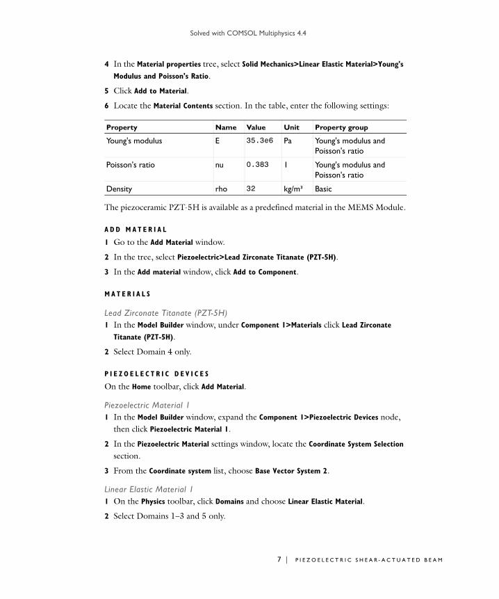
Solved with COMSOL Multiphysics 4.4
4 In the Material properties tree, select Solid Mechanics>Linear Elastic Material>Young's
Modulus and Poisson's Ratio.
5 Click Add to Material.
6 Locate the Material Contents section. In the table, enter the following settings:
The piezoceramic PZT-5H is available as a predefined material in the MEMS Module.
A D D M A T E R I A L
1 Go to the Add Material window.
2 In the tree, select Piezoelectric>Lead Zirconate Titanate (PZT-5H).
3 In the Add material window, click Add to Component.
M A T E R I A L S
Lead Zirconate Titanate (PZT-5H)1 In the Model Builder window, under Component 1>Materials click Lead Zirconate
Titanate (PZT-5H).
2 Select Domain 4 only.
P I E Z O E L E C T R I C D E V I C E S
On the Home toolbar, click Add Material.
Piezoelectric Material 11 In the Model Builder window, expand the Component 1>Piezoelectric Devices node,
then click Piezoelectric Material 1.
2 In the Piezoelectric Material settings window, locate the Coordinate System Selection section.
3 From the Coordinate system list, choose Base Vector System 2.
Linear Elastic Material 11 On the Physics toolbar, click Domains and choose Linear Elastic Material.
2 Select Domains 1–3 and 5 only.
Property Name Value Unit Property group
Young's modulus E 35.3e6 Pa Young's modulus and Poisson's ratio
Poisson's ratio nu 0.383 1 Young's modulus and Poisson's ratio
Density rho 32 kg/m³ Basic
7 | P I E Z O E L E C T R I C S H E A R - A C T U A T E D B E A M

Solved with COMSOL Multiphysics 4.4
8 | P I E Z
Fixed Constraint 11 On the Physics toolbar, click Boundaries and choose Fixed Constraint.
2 Select Boundaries 1, 4, and 7 only.
Electric Potential 11 On the Physics toolbar, click Boundaries and choose Electric Potential.
2 Select Boundary 16 only.
3 In the Electric Potential settings window, locate the Electric Potential section.
4 In the V0 edit field, type 20.
Ground 11 On the Physics toolbar, click Boundaries and choose Ground.
2 Select Boundary 17 only.
M E S H 1
Free Tetrahedral 11 In the Model Builder window, under Component 1 right-click Mesh 1 and choose Free
Tetrahedral.
2 Right-click Free Tetrahedral 1 and choose Build Selected.
The mesh consists of around 3600 elements.
O E L E C T R I C S H E A R - A C T U A T E D B E A M

Solved with COMSOL Multiphysics 4.4
S T U D Y 1
On the Home toolbar, click Compute.
R E S U L T S
Potential (pzd)1 In the Model Builder window, under Results>Potential (pzd) click Slice 1.
2 In the Slice settings window, locate the Plane Data section.
3 From the Plane list, choose ZX-planes.
4 On the 3D Plot Group toolbar, click Plot.
5 Click the Zoom In button on the Graphics toolbar.
Displacement (pzd)Follow the steps below to reproduce the plot shown in Figure 2.
1 In the Model Builder window, expand the Displacement (pzd) node, then click Surface
1.
2 In the Surface settings window, click Replace Expression in the upper-right corner of the Expression section. From the menu, choose Piezoelectric Devices (Solid
Mechanics)>Displacement>Displacement field (Material)>Displacement field, Z
component (w).
3 Locate the Expression section. From the Unit list, choose nm.
4 On the 3D Plot Group toolbar, click Plot.
5 Click the Zoom Extents button on the Graphics toolbar.
6 Click the Scene Light button on the Graphics toolbar.
9 | P I E Z O E L E C T R I C S H E A R - A C T U A T E D B E A M

Solved with COMSOL Multiphysics 4.4
10 | P I E
Z O E L E C T R I C S H E A R - A C T U A T E D B E A M
Solved with COMSOL Multiphysics 4.4
Con t a c t Ana l y s i s o f a S n ap Hook U s i n g a P ena l t y F o rmu l a t i o n
Introduction
Several numerical algorithms exist to handle structural contact problems. The one used as default in COMSOL Multiphysics is based on the so-called Augmented Lagrangian method.
Alternatively, you can use the Penalty method. It is based on the penalty factor formulation related to the penetration of the solid parts in contact. In some cases, this approach can result in faster computations and provide smoother convergence when compared to the Augmented Lagrangian method. The penalty method is however not suitable if accurate values of the contact pressure are important.
In this example, the purpose of the contact modeling is only to transmit correct contact forces in a global sense into the model, which is a situation well suited for using the penalty method.
Model Definition
The mechanical problem consists of the insertion of a snap hook into its groove. The objective is to compute the force needed to place the hook in the slot and then to remove it.
The geometry is shown in Figure 1. Due to the symmetry, you can study only a half of the original snap hook geometry.
1 | C O N T A C T A N A L Y S I S O F A S N A P H O O K U S I N G A P E N A L T Y F O R M U L A T I O N

Solved with COMSOL Multiphysics 4.4
2 | C O N
Figure 1: Geometry of the modeled half of the snap hook.
M A T E R I A L P R O P E R T I E S
You use a linear elastic material model for both the hook and groove. The groove is made of steel. The hook is made of a modified nylon material; the material parameters are given in the following table:
Since the steel is much stiffer than the nylon, it can be treated as rigid.
B O U N D A R Y C O N D I T I O N S
• The groove is fixed at its bottom surface.
A prescribed displacement boundary condition is applied at the bottom surface of the hook. The displacement in the x direction is gradually changed by using the parametric solver; the other two displacement components are zero.
• Two side boundaries within the xz plane use symmetry boundary conditions.
• All the other boundaries are free boundaries. However, several of them are selected as parts of a contact pair with the destination side being on the hook surface.
MATERIAL PARAMETER VALUE
Young’s modulus 10 GPa
Poisson’s number 0.35
Groove
Hook
T A C T A N A L Y S I S O F A S N A P H O O K U S I N G A P E N A L T Y F O R M U L A T I O N

Solved with COMSOL Multiphysics 4.4
Results
Figure 2 shows that the maximum penetration is less than 2 microns during the entire analysis. This is a good accuracy when compared to the geometry size.
Figure 2: Evolution of the maximum penetration for all position of the hook.
Note that the penetration is not constant since the contact force varies depending on the position of the hook
3 | C O N T A C T A N A L Y S I S O F A S N A P H O O K U S I N G A P E N A L T Y F O R M U L A T I O N

Solved with COMSOL Multiphysics 4.4
4 | C O N
The maximum effective stress levels are found at parameter step 0.83, which is just before the hook enters the groove, see Figure 3.
Figure 3: The effective stress levels in the hook just before it enters the groove.
T A C T A N A L Y S I S O F A S N A P H O O K U S I N G A P E N A L T Y F O R M U L A T I O N

Solved with COMSOL Multiphysics 4.4
Figure 4 shows the force required for the insertion and removal of the hook versus the parameter value. The hook is in its groove at the end of the simulation.
Figure 4: The mounting force as a function of the parameter step.
Model Library path: Structural_Mechanics_Module/Contact_and_Friction/snap_hook_penalty
Modeling Instructions
From the File menu, choose New.
N E W
1 In the New window, click the Model Wizard button.
M O D E L W I Z A R D
1 In the Model Wizard window, click the 3D button.
2 In the Select physics tree, select Structural Mechanics>Solid Mechanics (solid).
3 Click the Add button.
4 Click the Study button.
5 | C O N T A C T A N A L Y S I S O F A S N A P H O O K U S I N G A P E N A L T Y F O R M U L A T I O N

Solved with COMSOL Multiphysics 4.4
6 | C O N
5 In the tree, select Preset Studies>Stationary.
6 Click the Done button.
G L O B A L D E F I N I T I O N S
Parameters1 On the Home toolbar, click Parameters.
2 In the Parameters settings window, locate the Parameters section.
3 In the table, enter the following settings:
G E O M E T R Y 1
Import 11 On the Home toolbar, click Import.
2 In the Import settings window, locate the Import section.
3 Click the Browse button.
4 Browse to the model’s Model Library folder and double-click the file snap_hook_penalty.mphbin.
5 Click the Import button.
Rotate 11 On the Geometry toolbar, click Rotate.
2 Select the object imp1 only.
3 In the Rotate settings window, locate the Rotation Angle section.
4 In the Rotation edit field, type 90.
5 Locate the Axis of Rotation section. From the Axis type list, choose Cartesian.
6 In the x edit field, type 1.
7 In the z edit field, type 0.
8 Click the Build Selected button.
9 Click the Zoom Extents button on the Graphics toolbar.
D E F I N I T I O N S
1 On the Definitions toolbar, click Pairs and choose Contact Pair.
Name Expression Value Description
Displ_max 4.6[mm] 0.0046 m Maximum hook displacement
T A C T A N A L Y S I S O F A S N A P H O O K U S I N G A P E N A L T Y F O R M U L A T I O N

Solved with COMSOL Multiphysics 4.4
2 Select Boundaries 4, 6, and 7 only.
3 In the Pair settings window, locate the Destination Boundaries section.
4 Click the Active toggle button.
Select Boundaries 14, 15, 20, 22, and 23 only.
M A T E R I A L S
Material 11 In the Model Builder window, under Component 1 right-click Materials and choose
New Material.
2 In the Material settings window, locate the Material Contents section.
3 In the table, enter the following settings:
S O L I D M E C H A N I C S
To model the groove as a rigid material, constrain its displacement to zero.
Fixed Constraint 11 On the Physics toolbar, click Domains and choose Fixed Constraint.
2 Select Domain 1 only.
Prescribed Displacement 11 On the Physics toolbar, click Boundaries and choose Prescribed Displacement.
2 Select Boundary 30 only.
3 In the Prescribed Displacement settings window, locate the Prescribed Displacement section.
4 Select the Prescribed in x direction check box.
5 Select the Prescribed in y direction check box.
6 Select the Prescribed in z direction check box.
7 In the u0x edit field, type -Displ_max.
Symmetry 11 On the Physics toolbar, click Boundaries and choose Symmetry.
Property Name Value Unit Property group
Young's modulus E 10[GPa] Pa Basic
Poisson's ratio nu 0.35 1 Basic
Density rho 1150[kg/m^3] kg/m³ Basic
7 | C O N T A C T A N A L Y S I S O F A S N A P H O O K U S I N G A P E N A L T Y F O R M U L A T I O N

Solved with COMSOL Multiphysics 4.4
8 | C O N
2 Select Boundaries 5, 13, and 19 only.
Contact 11 On the Physics toolbar, click Pairs and choose Contact.
2 In the Contact settings window, locate the Pair Selection section.
3 In the Pairs list, select Contact Pair 1.
4 Locate the Contact Pressure Method section. From the list, choose Penalty.
M E S H 1
Add a structured mesh on the contact destination boundaries.
Mapped 11 In the Model Builder window, under Component 1 right-click Mesh 1 and choose
Mapped.
2 Select Boundaries 14, 15, 20, 22, and 23 only.
Distribution 11 Right-click Component 1>Mesh 1>Mapped 1 and choose Distribution.
2 Select Edges 27, 28, 39, and 48 only.
3 In the Distribution settings window, locate the Distribution section.
4 In the Number of elements edit field, type 10.
Distribution 21 Right-click Mapped 1 and choose Distribution.
2 Select Edges 31 and 45 only.
3 In the Distribution settings window, locate the Distribution section.
4 In the Number of elements edit field, type 4.
5 Click the Build Selected button.
Convert the quad mesh to triangles so that the rest of the geometry can be meshed using the free tetrahedral method.
Convert 11 In the Model Builder window, right-click Mesh 1 and choose More Operations>
Convert.
2 In the Convert settings window, locate the Geometric Entity Selection section.
3 From the Geometric entity level list, choose Boundary.
4 Select Boundaries 14, 15, 20, 22, and 23 only.
T A C T A N A L Y S I S O F A S N A P H O O K U S I N G A P E N A L T Y F O R M U L A T I O N

Solved with COMSOL Multiphysics 4.4
5 Click the Build Selected button.
Free Tetrahedral 11 In the Model Builder window, right-click Mesh 1 and choose Free Tetrahedral.
2 In the Free Tetrahedral settings window, locate the Domain Selection section.
3 From the Geometric entity level list, choose Domain.
4 Select Domains 2 and 3 only.
Size 11 Right-click Component 1>Mesh 1>Free Tetrahedral 1 and choose Size.
2 In the Size settings window, locate the Element Size section.
3 Click the Custom button.
4 Locate the Element Size Parameters section. Select the Maximum element size check box.
5 In the associated edit field, type 4e-4.
Size 21 Right-click Free Tetrahedral 1 and choose Size.
Refine the mesh on boundary where high stresses are expected.
2 In the Size settings window, locate the Geometric Entity Selection section.
3 From the Geometric entity level list, choose Boundary.
4 Select Boundary 25 only.
5 Locate the Element Size section. Click the Custom button.
6 Locate the Element Size Parameters section. Select the Maximum element size check box.
7 In the associated edit field, type 1e-4.
8 Click the Build Selected button.
As the groove is modeled as rigid, you only need to represent the surface that is in contact with the hook accurately.
Free Triangular 11 In the Model Builder window, right-click Mesh 1 and choose More Operations>
Free Triangular.
2 Select Boundary 2 only.
Size 11 Right-click Component 1>Mesh 1>Free Triangular 1 and choose Size.
9 | C O N T A C T A N A L Y S I S O F A S N A P H O O K U S I N G A P E N A L T Y F O R M U L A T I O N

Solved with COMSOL Multiphysics 4.4
10 | C O
2 In the Size settings window, locate the Element Size section.
3 From the Predefined list, choose Extremely coarse.
Distribution 11 Right-click Free Triangular 1 and choose Distribution.
2 Select Edges 5 and 13 only.
3 In the Distribution settings window, locate the Distribution section.
4 In the Number of elements edit field, type 10.
5 Click the Build Selected button.
Swept 1In the Model Builder window, right-click Mesh 1 and choose Swept.
Distribution 11 In the Model Builder window, under Component 1>Mesh 1 right-click Swept 1 and
choose Distribution.
2 In the Distribution settings window, locate the Distribution section.
3 In the Number of elements edit field, type 1.
4 Click the Build All button.
S T U D Y 1
Step 1: StationarySet up an auxiliary continuation sweep for the Disp_max parameter.
1 In the Model Builder window, under Study 1 click Step 1: Stationary.
2 In the Stationary settings window, click to expand the Study Extensions section.
3 Locate the Study Extensions section. Select the Auxiliary sweep check box.
4 Click Add.
5 In the table, enter the following settings:
6 Click to expand the Results While Solving section.
7 Select the Plot check box.
Solver 11 On the Study toolbar, click Show Default Solver.
Auxiliary parameter Parameter value list
Displ_max range(0.2,1e-2,1)*4.6[mm]
N T A C T A N A L Y S I S O F A S N A P H O O K U S I N G A P E N A L T Y F O R M U L A T I O N

Solved with COMSOL Multiphysics 4.4
2 In the Model Builder window, expand the Study 1>Solver Configurations>Solver
1>Stationary Solver 1 node, then click Parametric 1.
3 In the Parametric settings window, click to expand the Continuation section.
4 From the Predictor list, choose Linear.
5 On the Home toolbar, click Compute.
R E S U L T S
Derived Values1 On the Results toolbar, click Global Evaluation.
2 In the Global Evaluation settings window, locate the Expression section.
3 In the Expression edit field, type solid.gapmin_p1*(solid.gapmin_p1<0).
4 From the Unit list, choose um.
5 Select the Description check box.
6 In the associated edit field, type Minimum gap distance.
7 Click the Evaluate button.
TA B L E
In the Table window, click Table Graph.
R E S U L T S
Derived Values1 On the Results toolbar, click More Derived Values and choose
Integration>Surface Integration.
2 Select Boundary 30 only.
3 In the Surface Integration settings window, locate the Expression section.
4 In the Expression edit field, type -2*solid.RFx.
5 Select the Description check box.
6 In the associated edit field, type Total force.
7 Click the Evaluate button.
TA B L E
In the Table window, click Table Graph
11 | C O N T A C T A N A L Y S I S O F A S N A P H O O K U S I N G A P E N A L T Y F O R M U L A T I O N

Solved with COMSOL Multiphysics 4.4
12 | C O
N T A C T A N A L Y S I S O F A S N A P H O O K U S I N G A P E N A L T Y F O R M U L A T I O N
Solved with COMSOL Multiphysics 4.4
Th e rma l M i c r o a c t u a t o r
Introduction
This example model consists of a two-hot-arm thermal actuator made of polysilicon. The actuator is activated through thermal expansion. The temperature increase required to deform the two hot arms, and thus displace the actuator, is obtained through Joule heating (resistive heating). The greater expansion of the hot-arms, compared to the cold arm, causes a bending of the actuator.
The material properties of polysilicon are temperature dependent, which means that the involved physics phenomena are fully coupled. The electric current through the hot arms increases the temperature in the actuator, which in turn causes thermal expansion and changes the electrical conductivity of the material.
The actuator’s operation thus involves three coupled physics phenomena: electric current conduction, heat conduction with heat generation, and structural stresses and strains due to thermal expansion.
1 | T H E R M A L M I C R O A C T U A T O R

Solved with COMSOL Multiphysics 4.4
2 | T H E
Model Definition
Figure 1 shows the actuator’s parts and dimensions as well as its position on top of a substrate surface.
Figure 1: The thermal microactuator.
B O U N D A R Y C O N D I T I O N S A N D C O N S T R A I N T S
An electric potential is applied between the bases of the hot arms’ anchors. The cold arm anchor and all other surfaces are electrically insulated.
Figure 2: Electrical boundary conditions.
The temperature of the base of the three anchors and the three dimples is fixed to that of the substrate’s constant temperature. Because the structure is sandwiched, all other
Anchors
Hot arms
Cold armDimple
2 m
3 m
Substrate
Upper surface
240 m
Applied voltage
Ground
R M A L M I C R O A C T U A T O R

Solved with COMSOL Multiphysics 4.4
boundaries interact thermally with the surroundings by conduction through thin layers of air.
The heat transfer coefficient is given by the thermal conductivity of air divided by the distance to the surrounding surfaces for the system. This exercise uses different heat transfer coefficients for the actuator’s upper and other surfaces.
Figure 3: Heat-transfer boundary conditions.
All three arms are mechanically fixed at the base of the three anchors. The dimples can move freely in the plane of the substrate (the xy-plane in the figure) but do not move in the direction perpendicular to the substrate (the z direction).
Figure 4: Structural boundary conditions and constraints.
Fixed temperature
Fixed temperature
Heat flux = h(T-Tamb)T
Fixed temperature
Fixed
Fixed
Roller
3 | T H E R M A L M I C R O A C T U A T O R

Solved with COMSOL Multiphysics 4.4
4 | T H E
Results
Figure 5 shows the surface temperature distribution for the actuator. It also illustrates the displacement field through a deformation plot.
Figure 5: Temperature (surface) and displacement (deformation).
Model Library path: Structural_Mechanics_Module/Thermal-Structure_Interaction/thermal_actuator_tem_parameterized
Modeling Instructions
From the File menu, choose New.
N E W
1 In the New window, click the Model Wizard button.
M O D E L W I Z A R D
1 In the Model Wizard window, click the 3D button.
R M A L M I C R O A C T U A T O R
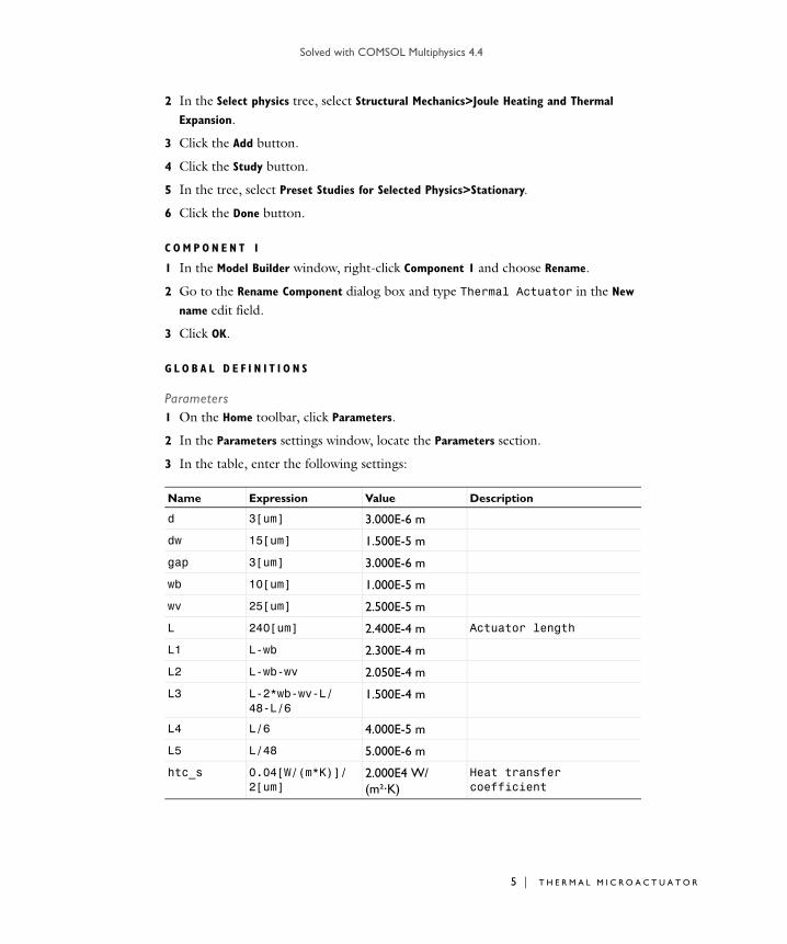
Solved with COMSOL Multiphysics 4.4
2 In the Select physics tree, select Structural Mechanics>Joule Heating and Thermal
Expansion.
3 Click the Add button.
4 Click the Study button.
5 In the tree, select Preset Studies for Selected Physics>Stationary.
6 Click the Done button.
C O M P O N E N T 1
1 In the Model Builder window, right-click Component 1 and choose Rename.
2 Go to the Rename Component dialog box and type Thermal Actuator in the New
name edit field.
3 Click OK.
G L O B A L D E F I N I T I O N S
Parameters1 On the Home toolbar, click Parameters.
2 In the Parameters settings window, locate the Parameters section.
3 In the table, enter the following settings:
Name Expression Value Description
d 3[um] 3.000E-6 m
dw 15[um] 1.500E-5 m
gap 3[um] 3.000E-6 m
wb 10[um] 1.000E-5 m
wv 25[um] 2.500E-5 m
L 240[um] 2.400E-4 m Actuator length
L1 L-wb 2.300E-4 m
L2 L-wb-wv 2.050E-4 m
L3 L-2*wb-wv-L/48-L/6
1.500E-4 m
L4 L/6 4.000E-5 m
L5 L/48 5.000E-6 m
htc_s 0.04[W/(m*K)]/2[um]
2.000E4 W/(m²·K)
Heat transfer coefficient
5 | T H E R M A L M I C R O A C T U A T O R

Solved with COMSOL Multiphysics 4.4
6 | T H E
G E O M E T R Y 1
Work Plane 11 On the Geometry toolbar, click Work Plane.
2 In the Model Builder window, under Thermal Actuator>Geometry 1 right-click Work
Plane 1 and choose Build Selected.
Plane GeometryRight-click Thermal Actuator >Geometry 1>Work Plane 1. In the Work Plane settings window, click Show Work Plane button.
Rectangle 11 In the Model Builder window, under Thermal Actuator>Geometry 1>Work Plane 1
right-click Plane Geometry and choose Rectangle.
2 In the Rectangle settings window, locate the Size section.
3 In the Width edit field, type L3.
4 In the Height edit field, type dw.
5 Locate the Position section. In the xw edit field, type L-L3.
6 Click the Build Selected button.
Rectangle 21 Right-click Plane Geometry and choose Rectangle.
2 In the Rectangle settings window, locate the Size section.
3 In the Width edit field, type L4.
4 In the Height edit field, type d.
5 Locate the Position section. In the xw edit field, type L-L3-L4.
6 In the yw edit field, type dw-d.
7 Click the Build Selected button.
8 Click the Zoom Extents button on the Graphics toolbar.
Rectangle 31 Right-click Plane Geometry and choose Rectangle.
htc_us 0.04[W/(m*K)]/100[um]
400.0 W/(m²·K) Heat transfer coefficient, upper surface
DV 5[V] 5.000 V Applied voltage
Name Expression Value Description
R M A L M I C R O A C T U A T O R

Solved with COMSOL Multiphysics 4.4
2 In the Rectangle settings window, locate the Size section.
3 In the Width edit field, type wb.
4 In the Height edit field, type dw.
5 Locate the Position section. In the xw edit field, type L-L3-L4-wb.
6 Click the Build Selected button.
7 Click the Zoom Extents button on the Graphics toolbar.
Rectangle 41 Right-click Plane Geometry and choose Rectangle.
2 In the Rectangle settings window, locate the Size section.
3 In the Width edit field, type L2.
4 In the Height edit field, type d.
5 Locate the Position section. In the xw edit field, type L-L2.
6 In the yw edit field, type dw+gap.
7 Click the Build Selected button.
Rectangle 51 Right-click Plane Geometry and choose Rectangle.
2 In the Rectangle settings window, locate the Size section.
3 In the Width edit field, type wb.
4 In the Height edit field, type dw+gap+d.
5 Locate the Position section. In the xw edit field, type L-L2-wb.
6 Click the Build Selected button.
7 Click the Zoom Extents button on the Graphics toolbar.
Rectangle 61 Right-click Plane Geometry and choose Rectangle.
2 In the Rectangle settings window, locate the Size section.
3 In the Width edit field, type L1.
4 In the Height edit field, type d.
5 Locate the Position section. In the xw edit field, type L-L1.
6 In the yw edit field, type dw+d+2*gap.
7 Click the Build Selected button.
8 Click the Zoom Extents button on the Graphics toolbar.
7 | T H E R M A L M I C R O A C T U A T O R

Solved with COMSOL Multiphysics 4.4
8 | T H E
Rectangle 71 Right-click Plane Geometry and choose Rectangle.
2 In the Rectangle settings window, locate the Size section.
3 In the Width edit field, type wb.
4 In the Height edit field, type dw+gap+d.
5 Locate the Position section. In the yw edit field, type dw+d+2*gap.
6 Click the Build Selected button.
7 Click the Zoom Extents button on the Graphics toolbar.
Rectangle 81 Right-click Plane Geometry and choose Rectangle.
2 In the Rectangle settings window, locate the Size section.
3 In the Width edit field, type d.
4 In the Height edit field, type gap.
5 Locate the Position section. In the xw edit field, type L-d.
6 In the yw edit field, type dw+gap+d.
7 Click the Build Selected button.
Rectangle 91 Right-click Plane Geometry and choose Rectangle.
2 In the Rectangle settings window, locate the Size section.
3 In the Width edit field, type d.
4 In the Height edit field, type gap.
5 Locate the Position section. In the xw edit field, type L-d.
6 In the yw edit field, type dw.
7 Click the Build Selected button.
Union 11 On the Work plane toolbar, click Union.
2 Press the Select All (Ctrl+A) button from the Graphics toolbar.
3 In the Union settings window, locate the Union section.
4 Clear the Keep interior boundaries check box.
5 Click the Build Selected button.
R M A L M I C R O A C T U A T O R

Solved with COMSOL Multiphysics 4.4
Fillet 11 On the Work plane toolbar, click Fillet.
2 In the Fillet settings window, locate the Radius section.
3 In the Radius edit field, type d/3.
4 On the object Union 1, select Points 1, 2, 4–9, 11–14, 16, 17, 19–23, and 28 only.
5 Click the Build Selected button.
Extrude 11 On the Geometry toolbar, click Extrude.
2 In the Extrude settings window, locate the Distances from Plane section.
3 In the table, enter the following settings:
4 Click the Build Selected button.
5 Click the Go to Default 3D View button on the Graphics toolbar.
Work Plane 21 On the Geometry toolbar, click Work Plane.
Distances (m)
2e-6
9 | T H E R M A L M I C R O A C T U A T O R

Solved with COMSOL Multiphysics 4.4
10 | T H
2 In the Model Builder window, under Thermal Actuator>Geometry 1 right-click Work
Plane 2 and choose Build Selected.
Plane Geometry1 Right-click Thermal Actuator>Geometry 1>Work Plane 2. In the Work Plane settings
window, click Show Work Plane button.
2 Click the Zoom Extents button on the Graphics toolbar.
Rectangle 11 In the Model Builder window, under Thermal Actuator>Geometry 1>Work Plane 2
right-click Plane Geometry and choose Rectangle.
2 In the Rectangle settings window, locate the Size section.
3 In the Width edit field, type wb-2*d.
4 In the Height edit field, type 2.5*(wb-2*d).
5 Locate the Position section. In the xw edit field, type d.
6 In the yw edit field, type (dw+d+2*gap)+(dw+gap+d)-2.5*(wb-2*d)-d.
7 Click the Build Selected button.
Rectangle 21 Right-click Plane Geometry and choose Rectangle.
2 In the Rectangle settings window, locate the Size section.
3 In the Width edit field, type wb-2*d.
4 In the Height edit field, type 2.5*(wb-2*d).
5 Locate the Position section. In the xw edit field, type L-L2-wb+d.
6 In the yw edit field, type d.
7 Click the Build Selected button.
Rectangle 31 Right-click Plane Geometry and choose Rectangle.
2 In the Rectangle settings window, locate the Size section.
3 In the Width edit field, type wb-2*d.
4 In the Height edit field, type 2.5*(wb-2*d).
5 Locate the Position section. In the xw edit field, type L-L3-L4-wb+d.
6 In the yw edit field, type d.
7 Click the Build Selected button.
E R M A L M I C R O A C T U A T O R

Solved with COMSOL Multiphysics 4.4
Fillet 11 On the Work plane toolbar, click Fillet.
2 In the Fillet settings window, locate the Radius section.
3 In the Radius edit field, type d/3.
Select all four vertices for all three rectangles as follows:
4 Click the Select Box button on the Graphics toolbar.
5 In the Graphics window, draw a box encompassing the three rectangles you just created.
6 Click the Build Selected button.
Circle 11 Right-click Plane Geometry and choose Circle.
2 In the Circle settings window, locate the Size and Shape section.
3 In the Radius edit field, type d/2.
4 Locate the Position section. In the xw edit field, type L-L3/4.
5 In the yw edit field, type dw/2.
6 Click the Build Selected button.
Circle 21 Right-click Plane Geometry and choose Circle.
2 In the Circle settings window, locate the Size and Shape section.
11 | T H E R M A L M I C R O A C T U A T O R

Solved with COMSOL Multiphysics 4.4
12 | T H
3 In the Radius edit field, type d/2.
4 Locate the Position section. In the xw edit field, type L-L3/2.
5 In the yw edit field, type dw/2.
6 Click the Build Selected button.
Circle 31 Right-click Plane Geometry and choose Circle.
2 In the Circle settings window, locate the Size and Shape section.
3 In the Radius edit field, type d/2.
4 Locate the Position section. In the xw edit field, type L-3*L3/4.
5 In the yw edit field, type dw/2.
6 Click the Build Selected button.
Extrude 21 On the Geometry toolbar, click Extrude.
2 In the Extrude settings window, locate the Distances from Plane section.
3 In the table, enter the following settings:
4 Select the Reverse direction check box.
5 Click the Build Selected button.
Union 11 On the Geometry toolbar, click Union.
2 Click the Zoom Extents button on the Graphics toolbar.
3 Select the objects ext1 and ext2 only.
4 Click the Build All Objects button.
D E F I N I T I O N S
Explicit 11 On the Definitions toolbar, click Explicit.
2 In the Explicit settings window, locate the Input Entities section.
3 From the Geometric entity level list, choose Boundary.
4 Select Boundaries 10, 30, 50, 70, 76, and 82 only.
Distances (m)
2e-6
E R M A L M I C R O A C T U A T O R

Solved with COMSOL Multiphysics 4.4
5 Right-click Thermal Actuator>Definitions>Explicit 1 and choose Rename.
6 Go to the Rename Explicit dialog box and type substrate contact in the New name edit field.
7 Click OK.
M A T E R I A L S
On the Home toolbar, click Add Material.
A D D M A T E R I A L
1 Go to the Add Material window.
2 In the Material tree, select MEMS>Semiconductors>Poly-Si.
3 In the Add material window, click Add to Component.
M A T E R I A L S
Poly-SiBy default, the first material you add applies on all domains so you can keep the Geometric Scope settings.
1 In the Model Builder window, under Thermal Actuator>Materials click Poly-Si.
2 In the Material settings window, locate the Material Contents section.
3 In the table, enter the following settings:
S O L I D M E C H A N I C S
Fixed Constraint 11 On the Physics toolbar, click Boundaries and choose Fixed Constraint.
2 Select Boundaries 10, 30, and 50 only.
Roller 11 On the Physics toolbar, click Boundaries and choose Roller.
2 Select Boundaries 70, 76, and 82 only.
Property Name Value Unit Property group
Electrical conductivity sigma 5e4 S/m Basic
13 | T H E R M A L M I C R O A C T U A T O R

Solved with COMSOL Multiphysics 4.4
14 | T H
H E A T TR A N S F E R I N S O L I D S
Heat Flux 11 On the Physics toolbar, click Boundaries and choose Heat Flux.
This boundary condition applies to all boundaries except the top-surface boundary and those in contact with the substrate. A Temperature condition on the substrate_contact boundaries will override this Heat Flux condition so you do not explicitly need to exclude those boundaries. In contrast, because the Heat Flux boundary condition is additive, you must explicitly exclude the top-surface boundary from the selection. Implement this selection as follows.
2 In the Heat Flux settings window, locate the Boundary Selection section.
3 From the Selection list, choose All boundaries.
4 In the Graphics window, click on the top surface to remove it from the selection.
5 Locate the Heat Flux section. Click the Inward heat flux button.
6 In the h edit field, type htc_s.
Heat Flux 21 On the Physics toolbar, click Boundaries and choose Heat Flux.
2 Select Boundary 4 only.
3 In the Heat Flux settings window, locate the Heat Flux section.
4 Click the Inward heat flux button.
5 In the h edit field, type htc_us.
Temperature 11 On the Physics toolbar, click Boundaries and choose Temperature.
2 In the Temperature settings window, locate the Boundary Selection section.
3 From the Selection list, choose substrate contact.
E L E C T R I C C U R R E N T S
Ground 11 On the Physics toolbar, click Boundaries and choose Ground.
2 Select Boundary 10 only.
Electric Potential 11 On the Physics toolbar, click Boundaries and choose Electric Potential.
2 Select Boundary 30 only.
E R M A L M I C R O A C T U A T O R

Solved with COMSOL Multiphysics 4.4
3 In the Electric Potential settings window, locate the Electric Potential section.
4 In the V0 edit field, type DV.
M E S H 1
Free Tetrahedral 1In the Model Builder window, under Thermal Actuator right-click Mesh 1 and choose Free Tetrahedral.
Size5 In the Size settings window, locate the Element Size section.
6 From the Predefined list, choose Fine.
7 Click the Custom button.
8 Locate the Element Size Parameters section. In the Maximum element growth rate edit field, type 1.2.
This setting makes the mesh more robust for parametric sweeps over the geometry length parameter L.
Size 11 In the Model Builder window, under Thermal Actuator >Mesh 1>Free Tetrahedral 1
click Size 1.
2 In the Size settings window, locate the Element Size section.
3 From the Predefined list, choose Finer.
4 Locate the Geometric Entity Selection section. From the Geometric entity level list, choose Boundary.
5 Select Boundaries 86–91 only.
6 Click the Build All button.
S T U D Y 1
Step 1: Stationary1 In the Model Builder window, under Study 1 click Step 1: Stationary.
2 In the Stationary settings window, locate the Study Settings section.
3 Select the Include geometric nonlinearity check box.
4 On the Home toolbar, click Compute.
15 | T H E R M A L M I C R O A C T U A T O R

Solved with COMSOL Multiphysics 4.4
16 | T H
R E S U L T S
Temperature (ht)1 Click the Go to Default 3D View button on the Graphics toolbar.
The third default plot shows the combined temperature field and deformation, compare it to that shown in Figure 5.
E R M A L M I C R O A C T U A T O R

Solved with COMSOL Multiphysics 4.4
L i n e a r Bu c k l i n g Ana l y s i s o f a T r u s s T owe r
Introduction
Trusses are commonly used to create light structures that can support heavy loads. When designing such a structure, it is important to ensure its safety. For a tower made of bars, buckling can cause the structure to collapse. This model shows how to compute the critical buckling load using a linear buckling analysis. The solution is compared with an analytical expression for critical load estimation for Euler buckling.
Model Definition
The model geometry consists of a 19-meters tall truss tower with a rectangular section. The critical buckling load is computed using the linear buckling analysis available in the Truss interface.
The geometry is the periodic structure represented in Figure 1 below. It consists of 19 blocks of trusses. Each block has width of 0.45 m, depth of 0.40 m and height of 1.0 m. The trusses that are perpendicular to the ground are thicker and have outer radius of 15 cm and inner radius of 10 cm. The remaining trusses have outer radius of
1 | L I N E A R B U C K L I N G A N A L Y S I S O F A TR U S S TO W E R

Solved with COMSOL Multiphysics 4.4
2 | L I N
10 cm and inner radius of 7 cm. The tower is made out of structural steel that one of the predefined materials in the material library.
Figure 1: Geometry of the truss tower.
The tower is fixed at the ground level and a vertical load is applied at the top.
One fourth of the unit load is applied at each point of the tower top so that the critical load factor returned by the linear buckling analysis corresponds to the load that would cause the collapse of the structure.
Results and Discussion
For a simple column the critical buckling load is given by the Euler buckling formula
where E is the Young’s modulus, I is the area moment of inertia, L is the unsupported length of the column and K is the column effective length factor.
For a column with one end fixed and the other end free to move laterally, K = 2.
Fc EI
KL 2----------------=
E A R B U C K L I N G A N A L Y S I S O F A TR U S S TO W E R
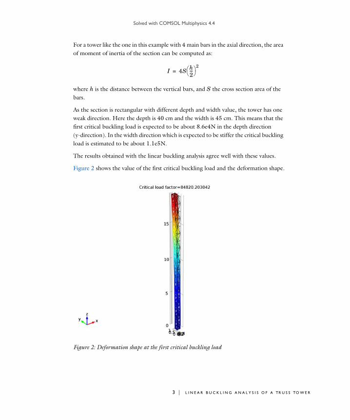
Solved with COMSOL Multiphysics 4.4
For a tower like the one in this example with 4 main bars in the axial direction, the area of moment of inertia of the section can be computed as:
where h is the distance between the vertical bars, and S the cross section area of the bars.
As the section is rectangular with different depth and width value, the tower has one weak direction. Here the depth is 40 cm and the width is 45 cm. This means that the first critical buckling load is expected to be about 8.6e4N in the depth direction (y-direction). In the width direction which is expected to be stiffer the critical buckling load is estimated to be about 1.1e5N.
The results obtained with the linear buckling analysis agree well with these values.
Figure 2 shows the value of the first critical buckling load and the deformation shape.
Figure 2: Deformation shape at the first critical buckling load
I 4S h2--- 2
=
3 | L I N E A R B U C K L I N G A N A L Y S I S O F A TR U S S TO W E R

Solved with COMSOL Multiphysics 4.4
4 | L I N
Figure 3 shows the value of the second critical buckling load and the deformation shape.
Figure 3: Deformation shape at the second critical buckling load
Note that the approximation given for the Euler buckling critical load is suitable for a tower structure when the height is significantly larger than the width or the depth.
Notes About the COMSOL Implementation
The default Truss interface implementation uses quadratic shape function so that the connection with other physics interfaces such as solid or shell is simplified. However with quadratic shape function an extra computational mid-point are included along the edges. A specific constraint is necessary to ensure the edge to remain straight. This is more demanding in term of computation.
For a model with only a Truss interface you can improve the performance by setting the shape discretization to linear, and by deactivating the Straight-edge constraint node. You must then control the mesh to have only 1 element per edge as shown in this model.
E A R B U C K L I N G A N A L Y S I S O F A TR U S S TO W E R

Solved with COMSOL Multiphysics 4.4
Model Library path: Structural_Mechanics_Module/Buckling/truss_tower_buckling
Modeling Instructions
From the File menu, choose New.
N E W
1 In the New window, click the Model Wizard button.
M O D E L W I Z A R D
1 In the Model Wizard window, click the 3D button.
2 In the Select physics tree, select Structural Mechanics>Truss (truss).
3 Click the Add button.
4 Click the Study button.
5 In the tree, select Preset Studies>Linear Buckling.
6 Click the Done button.
G L O B A L D E F I N I T I O N S
Parameters1 On the Home toolbar, click Parameters.
2 In the Parameters settings window, locate the Parameters section.
3 In the table, enter the following settings:
Name Expression Value Description
ro1 1.5[cm] 0.01500 m outer radius tube 1
ri1 1[cm] 0.01000 m inner radius tube 1
ro2 1[cm] 0.01000 m outer radius tube 2
ri2 0.7[cm] 0.007000 m inner radius tube 2
A1 pi*(ro1^2-ri1^2)
3.927E-4 m² area tube 1
A2 pi*(ro2^2-ri2^2)
1.602E-4 m² area tube 2
depth 0.4[m] 0.4000 m depth of the tower
5 | L I N E A R B U C K L I N G A N A L Y S I S O F A TR U S S TO W E R

Solved with COMSOL Multiphysics 4.4
6 | L I N
G E O M E T R Y 1
Block 11 On the Geometry toolbar, click Block.
2 In the Block settings window, locate the Size section.
3 In the Width edit field, type width.
4 In the Depth edit field, type depth.
5 In the Height edit field, type height.
6 Click the Build Selected button.
Bézier Polygon 11 On the Geometry toolbar, click More Primitives and choose Bézier Polygon.
2 In the Bézier Polygon settings window, locate the Polygon Segments section.
3 Find the Added segments subsection. Click the Add Linear button.
4 Find the Control points subsection. In row 1, set y to depth.
5 In row 2, set z to height.
6 Find the Added segments subsection. Click the Add Linear button.
7 Find the Control points subsection. In row 2, set x to width.
8 In row 2, set z to 0.
9 Find the Added segments subsection. Click the Add Linear button.
10 Find the Control points subsection. In row 2, set y to depth.
width 0.45[m] 0.4500 m width of the tower
height 1[m] 1.000 m height of the tower
n 10 10.00 Number of sections
L height*(2*n-1) 19.00 m Total height of the tower
I1 4*A1*(depth/2)^2
6.283E-5 m4 Area moment of inertia weak direction
Fc1 pi^2*200e9[Pa]*I1/(2*L)^2
8.589E4 N First critical buckling load
I2 4*A1*(width/2)^2
7.952E-5 m? Area moment of inertia stiffer direction
Fc2 pi^2*200e9[Pa]*I2/(2*L)^2
1.087E5 N Second critical buckling load
Name Expression Value Description
E A R B U C K L I N G A N A L Y S I S O F A TR U S S TO W E R

Solved with COMSOL Multiphysics 4.4
11 In row 2, set z to height.
12 Find the Added segments subsection. Click the Add Linear button.
13 Find the Control points subsection. In row 2, set x to 0.
14 In row 2, set z to 0.
Bézier Polygon 21 On the Geometry toolbar, click More Primitives and choose Bézier Polygon.
2 In the Bézier Polygon settings window, locate the Polygon Segments section.
3 Find the Added segments subsection. Click the Add Linear button.
4 Find the Control points subsection. In row 1, set y to depth.
5 In row 2, set x to width.
Bézier Polygon 31 On the Geometry toolbar, click More Primitives and choose Bézier Polygon.
2 In the Bézier Polygon settings window, locate the Polygon Segments section.
3 Find the Added segments subsection. Click the Add Linear button.
4 Find the Control points subsection. In row 1, set z to height.
5 In row 2, set x to width.
6 In row 2, set y to depth.
7 In row 2, set z to height.
8 Click the Build Selected button.
Convert to Curve 11 On the Geometry toolbar, click Conversions and choose Convert to Curve.
2 Click the Select All (Ctrl+A) button in the Graphics toolbar.
3 Click the Build Selected button.
Mirror 11 On the Geometry toolbar, click Mirror.
2 In the Mirror settings window, locate the Input section.
3 Select the object cur1 only.
4 Select the Keep input objects check box.
5 Locate the Point on Plane of Reflection section. In the z edit field, type height.
6 Click the Build Selected button.
7 | L I N E A R B U C K L I N G A N A L Y S I S O F A TR U S S TO W E R

Solved with COMSOL Multiphysics 4.4
8 | L I N
Array 11 On the Geometry toolbar, click Array.
2 In the Array settings window, locate the Input section.
3 Select the object cur1 only.
4 In the Array settings window, locate the Size section.
5 In the z size edit field, type n.
6 Locate the Displacement section. In the z edit field, type 2*height.
7 Click the Build Selected button.
8 Click the Go to Default 3D View button on the Graphics toolbar.
Array 21 On the Geometry toolbar, click Array.
2 In the Array settings window, locate the Input section.
3 Select the object mir1 only.
4 In the Array settings window, locate the Size section.
5 In the z size edit field, type n-1.
6 Locate the Displacement section. In the z edit field, type 2*height.
7 Click the Build Selected button.
8 Click the Zoom Extents button on the Graphics toolbar.
M A T E R I A L S
On the Home toolbar, click Add Material.
A D D M A T E R I A L
1 Go to the Add Material window.
2 In the tree, select Built-In>Structural steel.
3 In the Add material window, click Add to Component.
4 In the Material settings window, locate the Geometric Entity Selection section. At the Geometric entity level list select Edge. At the Selection list select All Edges.
5 On the Home toolbar, click Add Material to close the add material window.
In the Model Builder window’s toolbar, click the Show button and select Discretization in the menu.
E A R B U C K L I N G A N A L Y S I S O F A TR U S S TO W E R

Solved with COMSOL Multiphysics 4.4
TR U S S
1 In the Model Builder window, under Component 1 click Truss.
2 In the Truss settings window, click to expand the Discretization section.
3 From the Displacement field list, choose Linear.
Cross Section Data 11 In the Model Builder window, under Component 1>Truss click Cross Section Data 1.
2 In the Cross Section Data settings window, locate the Cross Section Data section.
3 In the A edit field, type A2.
Cross Section Data 21 On the Physics toolbar, click Edges and choose Cross Section Data.
2 Select all the vertical edges. You can use the Select box tool for easier selection.
3 In the Cross Section Data settings window, locate the Cross Section Data section.
4 In the A edit field, type A1.
Straight Edge Constraint 1In the Model Builder window, under Component 1>Truss right-click Straight Edge
Constraint 1 and choose Disable.
Pinned 11 On the Physics toolbar, click Points and choose Pinned.
2 Select Points 1, 21, 41, and 61, located at the bottom of the tower.
Point Load 11 On the Physics toolbar, click Points and choose Point Load.
2 Select Points 20, 40, 60, and 80, located at the top of the tower.
3 In the Point Load settings window, locate the Point Load section.
4 Specify the Fp vector as
0 x
0 y
-1/4 z
9 | L I N E A R B U C K L I N G A N A L Y S I S O F A TR U S S TO W E R

Solved with COMSOL Multiphysics 4.4
10 | L I N
M E S H 1
Edge 11 In the Model Builder window, under Component 1 right-click Mesh 1 and choose More
Operations>Edge.
2 In the Edge settings window, locate the Edge Selection section.
3 From the Selection list, choose All edges.
Distribution 11 Right-click Component 1>Mesh 1>Edge 1 and choose Distribution.
2 In the Distribution settings window, locate the Distribution section.
3 In the Number of elements edit field, type 1.
S T U D Y 1
Step 2: Linear Buckling1 In the Model Builder window, under Study 1 click Step 2: Linear Buckling.
2 In the Linear Buckling settings window, locate the Study Settings section.
3 In the Desired number of buckling modes edit field, type 2.
4 On the Home toolbar, click Compute.
R E S U L T S
Mode Shape (truss)1 In the Model Builder window, expand the Mode Shape (truss) node, then click Line 1.
2 In the Line settings window, click to expand the Title section.
3 From the Title type list, choose None.
4 Locate the Coloring and Style section. Clear the Color legend check box.
5 On the Mode Shape (truss) toolbar, click Plot.
6 Click the Zoom Extents button on the Graphics toolbar.
7 In the Model Builder window, click Mode Shape (truss).
8 In the 3D Plot Group settings window, locate the Data section.
9 From the Critical load factor list, choose 1.071956e5.
10 On the Mode Shape (truss) toolbar, click Plot.
E A R B U C K L I N G A N A L Y S I S O F A TR U S S TO W E R
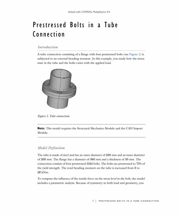
Solved with COMSOL Multiphysics 4.4
P r e s t r e s s e d Bo l t s i n a Tub e Conn e c t i o n
Introduction
A tube connection consisting of a flange with four prestressed bolts (see Figure 1) is subjected to an external bending moment. In this example, you study how the stress state in the tube and the bolts varies with the applied load.
Figure 1: Tube connection.
Note: This model requires the Structural Mechanics Module and the CAD Import Module.
Model Definition
The tube is made of steel and has an outer diameter of 220 mm and an inner diameter of 200 mm. The flange has a diameter of 360 mm and a thickness of 30 mm. The connection consists of four prestressed M24 bolts. The bolts are prestressed to 75% of the yield strength. The total bending moment on the tube is increased from 0 to 26 kNm.
To compute the influence of the tensile force on the stress level in the bolt, the model includes a parametric analysis. Because of symmetry in both load and geometry, you
1 | P R E S T R E S S E D B O L T S I N A TU B E C O N N E C T I O N

Solved with COMSOL Multiphysics 4.4
2 | P R E
only need to analyze one half of one of the flanges. The geometry has been created in the CAD software SolidWorks® and is available as an IGES file.
Two contact regions are modeled. One contact pair acts between the bottom surface of the flange and the top surface of an additional fixed solid which supplies the symmetry condition with respect to contact. The other contact pair acts between the washers under the bolt heads and the flange. The possibility to automatically detect potential contact surfaces is used when creating the contact pairs.
Results and Discussion
After the pretension step, there is a tensile stress in the bolt, and compressive stress in the flange under the bolt. This is illustrated in Figure 2.
Figure 2: The axial stress after the pretension step.
The general stress state at maximum external load is shown in Figure 3. In addition to the stress that has increased in the fillet between tube and flange, additional features are visible. The stress state in the bolt on the tensile side has increased significantly and is no longer axisymmetric. Furthermore, a stress of the order of 300 MPa has developed in the fillet between the tube and the flange.This stress is caused by local
S T R E S S E D B O L T S I N A TU B E C O N N E C T I O N

Solved with COMSOL Multiphysics 4.4
bending, since the flange no longer is in contact with the mating surface at the tensile side.
Figure 3: Effective stress at maximum external load.
The applied external load in this example overloads the bolted joint. Up to about half the full load, it works fairly well, but then the contact between the two mating flanges start to open up on the tensile side. This is displayed in Figure 4. Actually, the conditions are even worse than the average force indicates. The bolt is subjected to bending with a non-uniform stress distribution over the cross section. The maximum stress has increased from the prestress value of 75% of the yield stress to 88% of the yield stress, and the progression is fast. The development of the axial stress in two points on opposite sides of the bolt is displayed in Figure 5. The points are located in the x-z symmetry plane. One point is as close to the tube centerline as possible and the other as far out as possible.
3 | P R E S T R E S S E D B O L T S I N A TU B E C O N N E C T I O N

Solved with COMSOL Multiphysics 4.4
4 | P R E
Figure 4: The bolt force as a function of the tensile force.
Figure 5: The development of the bolt stress at two different positions in the cross section.
S T R E S S E D B O L T S I N A TU B E C O N N E C T I O N

Solved with COMSOL Multiphysics 4.4
The plots of the contact pressure between the mating flanges are shown in Figure 6 and Figure 7. By comparing these two figures, it is clear that the contact pressure shifts away from the initially prestressed area which at the peak load becomes almost stress free. This indicates that there are too few bolts that connect the two parts with each other.
Figure 6: Contact pressure between flanges after pretensioning the bolts.
5 | P R E S T R E S S E D B O L T S I N A TU B E C O N N E C T I O N

Solved with COMSOL Multiphysics 4.4
6 | P R E
Figure 7: Contact pressure between the flanges at full external load.
Notes About the COMSOL Implementation
The analysis is performed in two steps and therefore represented by two studies. In the first step, the effects of pretensioning the bolt are computed, and in the second step the external load on the tube is applied as a parametric sweep.
The prestress in the bolts is introduced using the built-in Bolt Pre-tension feature. This feature will create one degree of freedom for each bolt, which can be interpreted as the shortening of the bolt caused by prestress. This degree of freedom is then kept fixed under service loads.
In order to keep the solution time down, the mesh used in the model is coarse, and it probably needs a refinement if one needs to obtain accurate quantitative results for stresses.
S T R E S S E D B O L T S I N A TU B E C O N N E C T I O N

Solved with COMSOL Multiphysics 4.4
Model Library path: Structural_Mechanics_Module/Contact_and_Friction/tube_connection
Modeling Instructions
From the File menu, choose New.
N E W
1 In the New window, click the Model Wizard button.
M O D E L W I Z A R D
1 In the Model Wizard window, click the 3D button.
2 In the Select Physics tree, select Structural Mechanics>Solid Mechanics (solid).
3 Click the Add button.
4 Click the Study button.
5 In the tree, select Preset Studies>Stationary.
6 Click the Done button.
G L O B A L D E F I N I T I O N S
Parameters1 On the Home toolbar, click Parameters.
2 In the Parameters settings window, locate the Parameters section.
3 In the table, enter the following settings:
Name Expression Value Description
Di_wash 25[mm] 0.02500 m Washer inner diameter
Do_wash 45[mm] 0.04500 m Washer outer diameter
T_wash 4[mm] 0.004000 m Washer thickness
Do_bolthead 38[mm] 0.03800 m Bolthead diameter
H_bolthead 15[mm] 0.01500 m Bolthead height
As_bolt 353[mm^2] 3.530E-4 m² Stress area of bolt
Ds_bolt sqrt(4/pi*As_bolt)
0.02120 m Effective bolt diameter
7 | P R E S T R E S S E D B O L T S I N A TU B E C O N N E C T I O N

Solved with COMSOL Multiphysics 4.4
8 | P R E
G E O M E T R Y 1
Import 11 On the Home toolbar, click Import.
2 In the Import settings window, locate the Import section.
3 Click the Browse button.
4 Browse to the model’s Model Library folder and double-click the file tube_connection.igs.
5 Click the Import button.
6 Click the Build Selected button.
7 Click the Zoom Extents button on the Graphics toolbar.
Remove half the geometry to make use of the symmetry.
Block 11 On the Geometry toolbar, click Block.
2 In the Block settings window, locate the Size section.
3 In the Width edit field, type 0.5.
4 In the Depth edit field, type 0.3.
5 In the Height edit field, type 0.3.
6 Locate the Position section. In the x edit field, type -0.25.
7 In the y edit field, type -0.05.
R_bc 150[mm] 0.1500 m Bolt circle radius
Do_pipe 0.22[m] 0.2200 m Pipe outer diameter
Di_pipe 0.20[m] 0.2000 m Pipe inner diameter
Wb pi/32*(Do_pipe^4-Di_pipe^4)/Do_pipe
3.314E-4 m³ Pipe bending resistance
M_appl 26E3[N*m] 2.600E4 N·m Applied bending moment
ps 1 1.000 Parameter for spring relaxation
lp 0 0 Loading parameter
Name Expression Value Description
S T R E S S E D B O L T S I N A TU B E C O N N E C T I O N

Solved with COMSOL Multiphysics 4.4
Difference 11 On the Geometry toolbar, click Difference.
2 Select the object imp1 only.
3 In the Difference settings window, locate the Difference section.
4 Select the Objects to subtract toggle button.
5 Select the object blk1 only.
6 Click the Build Selected button.
7 Click the Zoom Extents button on the Graphics toolbar.
Next, create the bolts.
8 On the Geometry toolbar, click Work Plane.
Plane GeometryClick the Zoom Extents button on the Graphics toolbar.
Bézier Polygon 11 In the Model Builder window, under Component 1>Geometry 1>Work Plane 1
right-click Plane Geometry and choose Bézier Polygon.
2 In the Bézier Polygon settings window, locate the Polygon Segments section.
3 Find the Added segments subsection. Click the Add Linear button.
4 Find the Control points subsection. In row 1, set xw to R_bc.
5 In row 1, set yw to -0.03.
6 In row 2, set xw to R_bc+Ds_bolt/2.
7 In row 2, set yw to -0.03.
8 Find the Added segments subsection. Click the Add Linear button.
9 Find the Control points subsection. In row 2, set yw to T_wash.
10 Find the Added segments subsection. Click the Add Linear button.
11 Find the Control points subsection. In row 2, set xw to R_bc+Di_wash/2.
12 Find the Added segments subsection. Click the Add Linear button.
13 Find the Control points subsection. In row 2, set yw to 0.
14 Find the Added segments subsection. Click the Add Linear button.
15 Find the Control points subsection. In row 2, set xw to R_bc+Do_wash/2.
16 Find the Added segments subsection. Click the Add Linear button.
17 Find the Control points subsection. In row 2, set yw to T_wash.
9 | P R E S T R E S S E D B O L T S I N A TU B E C O N N E C T I O N

Solved with COMSOL Multiphysics 4.4
10 | P R
18 Find the Added segments subsection. Click the Add Linear button.
19 Find the Control points subsection. In row 2, set xw to R_bc+Do_bolthead/2.
20 Find the Added segments subsection. Click the Add Linear button.
21 Find the Control points subsection. In row 2, set yw to T_wash+H_bolthead.
22 Find the Added segments subsection. Click the Add Linear button.
23 Find the Control points subsection. In row 2, set xw to R_bc.
24 Find the Added segments subsection. Click the Add Linear button.
25 Find the Control points subsection. Click the Close Curve button.
26 Click the Build Selected button.
Make sure that there is an internal slit boundary in the bolt.
Rectangle 11 Right-click Plane Geometry and choose Rectangle.
2 In the Rectangle settings window, locate the Position section.
3 In the xw edit field, type R_bc.
4 In the yw edit field, type -0.03.
5 Locate the Size section. In the Width edit field, type Ds_bolt/2.
6 In the Height edit field, type 10[mm].
7 Click the Build Selected button.
Revolve 11 On the Geometry toolbar, click Revolve.
2 In the Revolve settings window, locate the Revolution Angles section.
3 In the End angle edit field, type 180.
4 Locate the Revolution Axis section. Find the Point on the revolution axis subsection. In the xw edit field, type R_bc.
5 Click the Build Selected button.
Duplicate to three bolts.
Rotate 11 On the Geometry toolbar, click Rotate.
2 Select the object rev1 only.
3 In the Rotate settings window, locate the Input section.
4 Select the Keep input objects check box.
E S T R E S S E D B O L T S I N A TU B E C O N N E C T I O N

Solved with COMSOL Multiphysics 4.4
5 Locate the Rotation Angle section. In the Rotation edit field, type 90.
6 Locate the Axis of Rotation section. From the Axis type list, choose y-axis.
7 Click the Build Selected button.
Mirror 11 On the Geometry toolbar, click Mirror.
2 Select the objects rot1 and rev1 only.
3 In the Mirror settings window, locate the Input section.
4 Select the Keep input objects check box.
5 Locate the Normal Vector to Plane of Reflection section. In the x edit field, type 1.
6 In the z edit field, type 0.
7 Click the Build Selected button.
Union 11 On the Geometry toolbar, click Union.
2 Select the objects rot1 and mir1(2) only.
3 Click the Build Selected button.
Create a rigid block to act as symmetry condition for the contact modeling.
Block 21 On the Geometry toolbar, click Block.
2 In the Block settings window, locate the Size section.
3 In the Width edit field, type 0.4.
4 In the Depth edit field, type 0.01.
5 In the Height edit field, type 0.25.
6 Locate the Position section. In the x edit field, type -0.2.
7 In the y edit field, type -0.04.
8 In the z edit field, type -0.2.
9 Click the Build Selected button.
Form Union1 In the Model Builder window, under Component 1>Geometry 1 click Form Union.
2 In the Form Union/Assembly settings window, locate the Form Union/Assembly section.
3 From the Action list, choose Form an assembly.
4 From the Pair type list, choose Contact pair.
11 | P R E S T R E S S E D B O L T S I N A TU B E C O N N E C T I O N

Solved with COMSOL Multiphysics 4.4
12 | P R
5 On the Home toolbar, click Build All.
Ignore Edges 11 On the Geometry toolbar, click Virtual Operations and choose Ignore Edges.
2 On the object fin, select Edges 27 and 47 only.
This will improve the mesh at the transition to the fillet, where large stresses can be expected.
This completes the geometry modeling stage. The geometry should now look like that in the figure below.
M A T E R I A L S
On the Home toolbar, click Add Material.
A D D M A T E R I A L
1 Go to the Add Material window.
2 In the tree, select Built-In>Structural steel.
3 In the Add Material window, click Add to Component.
S O L I D M E C H A N I C S
Fixed Constraint 11 On the Physics toolbar, click Domains and choose More>Fixed Constraint.
E S T R E S S E D B O L T S I N A TU B E C O N N E C T I O N

Solved with COMSOL Multiphysics 4.4
2 Select Domain 1 only.
Symmetry 11 On the Physics toolbar, click Boundaries and choose Solid Mechanics>Symmetry.
2 Select Boundaries 7, 12, 21, 23, 24, 33, 34, 37, 39, 42, 66, 67, 73, 76, 98, 107, 108, 111, 113, and 116 only.
Add a constraint suppressing any rigid body translation in the x direction.
3 Prescribed Displacement 1
1 On the Physics toolbar, click Points and choose Prescribed Displacement.
2 Select Point 22 only.
3 In the Prescribed Displacement settings window, locate the Prescribed Displacement section.
4 Select the Prescribed in x direction check box.
Bolt Pre-Tension 11 On the Physics toolbar, click Global and choose Bolt Pre-Tension.
2 In the Bolt Pre-Tension settings window, locate the Bolt Pre-Tension section.
3 From the Pre-tension type list, choose Pre-tension stress.
4 In the p edit field, type 800[MPa]*0.8*0.75.
Bolt Selection 11 In the Model Builder window, expand the Bolt Pre-Tension 1 node, then click Bolt
Selection 1.
2 Select Boundaries 36 and 40 only.
Bolt Selection 21 In the Model Builder window, under Component 1>Solid Mechanics right-click Bolt
Pre-Tension 1 and choose Bolt Selection.
2 In the Bolt Selection settings window, locate the Bolt Selection section.
3 In the Bolt label edit field, type Bolt_2.
4 Select Boundaries 70, 71, 79, and 82 only.
Bolt Selection 31 Right-click Bolt Pre-Tension 1 and choose Bolt Selection.
2 In the Bolt Selection settings window, locate the Bolt Selection section.
3 In the Bolt label edit field, type Bolt_3.
13 | P R E S T R E S S E D B O L T S I N A TU B E C O N N E C T I O N

Solved with COMSOL Multiphysics 4.4
14 | P R
4 Select Boundaries 110 and 114 only.
Spring Foundation 11 On the Physics toolbar, click Domains and choose More>Spring Foundation.
2 Select Domains 2–10 only.
3 In the Spring Foundation settings window, locate the Spring section.
4 From the Spring type list, choose Total spring constant.
5 Specify the ktot vector as
Before creating the contact conditions, check the automatically created contact pairs. The automatically generated source and destination selections are good in this case, so there is no need to change anything. Three pairs (ap2, ap3, and ap4) are not needed. You can delete them to clean up the model, but this is not necessary.
S O L I D M E C H A N I C S
Contact 11 On the Physics toolbar, click Pairs and choose Solid Mechanics>Contact.
2 In the Contact settings window, locate the Pair Selection section.
3 In the Pairs list, select Contact Pair 1.
4 Locate the Penalty Factor section. From the Tuned for list, choose Speed.
Contact 21 On the Physics toolbar, click Pairs and choose Solid Mechanics>Contact.
2 In the Contact settings window, locate the Pair Selection section.
3 In the Pairs list, choose Contact Pair 5, Contact Pair 6, and Contact Pair 7.
4 Locate the Penalty Factor section. From the Tuned for list, choose Speed.
Friction 11 Right-click Component 1>Solid Mechanics>Contact 2 and choose Friction.
2 In the Friction settings window, locate the Friction section.
3 In the stat edit field, type 0.15.
1e10*(1-ps) x
1e12*(1-ps) y
1e10*(1-ps) z
E S T R E S S E D B O L T S I N A TU B E C O N N E C T I O N

Solved with COMSOL Multiphysics 4.4
Boundary Load 11 On the Physics toolbar, click Boundaries and choose Solid Mechanics>Boundary Load.
2 Select Boundary 14 only.
3 In the Boundary Load settings window, locate the Force section.
4 Specify the FA vector as
M E S H 1
1 In the Model Builder window, under Component 1 click Mesh 1.
2 In the Mesh settings window, locate the Mesh Settings section.
3 From the Sequence type list, choose User-controlled mesh.
Size1 In the Model Builder window, under Component 1>Mesh 1 click Size.
2 In the Size settings window, locate the Element Size section.
3 From the Predefined list, choose Fine.
Size 11 In the Model Builder window, under Component 1>Mesh 1 right-click Free Tetrahedral
1 and choose Size.
2 In the Size settings window, locate the Geometric Entity Selection section.
3 From the Geometric entity level list, choose Boundary.
4 Select Boundaries 13 and 20 only.
5 Locate the Element Size section. From the Predefined list, choose Fine.
6 Click the Build All button.
Refine the mesh on the destination boundaries of the contact pairs.
Size 21 Right-click Free Tetrahedral 1 and choose Size.
2 In the Size settings window, locate the Geometric Entity Selection section.
3 From the Geometric entity level list, choose Boundary.
4 Select Boundaries 26, 43, 52, 53, 84, 87, 100, and 117 only.
0 x
lp*M_appl/Wb*X/(Do_pipe/2) y
0 z
15 | P R E S T R E S S E D B O L T S I N A TU B E C O N N E C T I O N

Solved with COMSOL Multiphysics 4.4
16 | P R
5 Locate the Element Size section. From the Predefined list, choose Finer.
6 Click the Build All button.
Since the block is rigid, one brick element is enough to represent it.
Mapped 11 In the Model Builder window, right-click Mesh 1 and choose More
Operations>Mapped.
2 Select Boundary 5 only.
Distribution 11 Right-click Component 1>Mesh 1>Mapped 1 and choose Distribution.
2 Select Edges 6 and 8 only.
3 In the Distribution settings window, locate the Distribution section.
4 In the Number of elements edit field, type 1.
5 In the Model Builder window, right-click Mesh 1 and choose Swept.
Free Tetrahedral 11 In the Model Builder window, under Component 1>Mesh 1 click Free Tetrahedral 1.
2 In the Free Tetrahedral settings window, locate the Domain Selection section.
3 From the Geometric entity level list, choose Domain.
4 Remove Domain 1 from the selection.
5 Click the Build All button.
E S T R E S S E D B O L T S I N A TU B E C O N N E C T I O N

Solved with COMSOL Multiphysics 4.4
The mesh should now look as in the figure below
S T U D Y 1
1 In the Model Builder window, right-click Study 1 and choose Rename.
2 Go to the Rename Study dialog box and type Study 1: Prestress in the New name edit field.
3 Click OK.
S T U D Y 1 : P R E S T R E S S
Step 1: Stationary1 In the Stationary settings window, click to expand the Study Extensions section.
2 Locate the Study Extensions section. Select the Auxiliary sweep check box.
3 Click Add.
4 In the table, enter the following settings:
Solver 11 On the Study toolbar, click Show Default Solver.
Auxiliary parameter Parameter value list
ps 0 1
17 | P R E S T R E S S E D B O L T S I N A TU B E C O N N E C T I O N

Solved with COMSOL Multiphysics 4.4
18 | P R
2 In the Model Builder window, expand theStudy 1: Prestress>Solver Configurations>Solver 1>Dependent Variables 1 node, then click Displacement field (Material) (comp1.u).
3 In the Field settings window, locate the Scaling section.
4 In the Scale edit field, type 1e-4.
The default scale for the displacements is 1% of the model size. This is significantly more than can be expected here.
5 On the Home toolbar, click Compute.
R E S U L T S
Stress (solid)Reproduce the plot in Figure 2 with the following steps.
1 In the Model Builder window, expand the Stress (solid) node, then click Surface 1.
2 In the Surface settings window, click Replace Expression in the upper-right corner of the Expression section. From the menu, chooseSolid Mechanics>Stress>Stress tensor (Spatial)>Stress tensor, y component (solid.sy).
3 Click to expand the Range section. Select the Manual color range check box.
4 In the Minimum edit field, type -3e8.
5 In the Maximum edit field, type 5e8.
6 In the Model Builder window, expand the Results>Stress (solid)>Surface 1 node, then click Deformation.
7 In the Deformation settings window, locate the Scale section.
8 In the Scale factor edit field, type 50.
9 In the Model Builder window, under Results>Stress (solid) right-click Surface 1 and choose Filter.
10 In the Filter settings window, locate the Element Selection section.
11 In the Logical expression for inclusion edit field, type dom>6.
This removes the rigid block from the plot, since it contains the boundaries 1 to 6.
12 On the Stress (solid) toolbar, click Plot.
Add a new study for the loading of the tube.
R O O T
On the Home toolbar, click More Windows and choose Add Study.
E S T R E S S E D B O L T S I N A TU B E C O N N E C T I O N

Solved with COMSOL Multiphysics 4.4
A D D S T U D Y
1 Go to the Add Study window.
2 Find the Studies subsection. In the tree, select Preset Studies>Stationary.
3 In the Add study window, click Add Study.
S T U D Y 2
Step 1: Stationary1 In the Model Builder window, right-click Study 2 and choose Rename.
2 Go to the Rename Study dialog box and type Study 2: External load in the New
name edit field.
3 Click OK.
S T U D Y 2 : E X T E R N A L L O A D
Step 1: Stationary1 In the Stationary settings window, locate the Study Extensions section.
2 Select the Auxiliary sweep check box.
3 Click Add.
4 In the table, enter the following settings:
5 Click to expand the Values of dependent variables section. Locate the Values of
Dependent Variables section. Select the Initial values of variables solved for check box.
6 From the Method list, choose Solution.
7 From the Study list, choose Study 1: Prestress, Stationary.
8 Select the Values of variables not solved for check box.
9 From the Method list, choose Solution.
10 From the Study list, choose Study 1: Prestress, Stationary.
The pre-deformation in the bolts is to be kept constant during the application of the external load, so it should not be solved for.
Solver 21 On the Study toolbar, click Show Default Solver.
Auxiliary parameter Parameter value list
lp range(0.2,0.2,1)
19 | P R E S T R E S S E D B O L T S I N A TU B E C O N N E C T I O N

Solved with COMSOL Multiphysics 4.4
20 | P R
2 In the Model Builder window, underStudy 2: External load>Solver Configurations>Solver 2 click Dependent Variables 1.
3 In the Dependent Variables settings window, locate the General section.
4 From the Defined by study step list, choose User defined.
5 In the Model Builder window, underStudy 2: External load>Solver Configurations>Solver 2>Dependent Variables 1 click Pre-deformation (comp1.solid.pblt1.sblt1.d_pre).
6 In the State settings window, locate the General section.
7 Clear the Solve for this state check box.
8 Repeat the same steps for the variables comp1.solid.pblt1.sblt2.d_pre and comp1.solid.pblt1.sblt3.d_pre .
9 In the Model Builder window, underStudy 2: External load>Solver Configurations>Solver 2>Dependent Variables 1 click Displacement field (Material) (comp1.u).
10 In the Field settings window, locate the Scaling section.
11 In the Scale edit field, type 1e-4.
12 On the Home toolbar, click Compute.
R E S U L T S
Stress (solid) 1The following steps reproduce the plot in Figure 3:
1 In the Model Builder window, expand the Stress (solid) 1 node, then click Surface 1.
2 In the Surface settings window, locate the Range section.
3 Select the Manual color range check box.
4 In the Maximum edit field, type 4e8.
5 In the Model Builder window, under Results>Stress (solid) 1>Surface 1 click Deformation.
6 In the Deformation settings window, locate the Scale section.
7 In the Scale factor edit field, type 50.
8 In the Model Builder window, under Results>Stress (solid) 1 right-click Surface 1 and choose Filter.
9 In the Filter settings window, locate the Element Selection section.
10 In the Logical expression for inclusion edit field, type dom>6.
E S T R E S S E D B O L T S I N A TU B E C O N N E C T I O N

Solved with COMSOL Multiphysics 4.4
11 Click the Plot button.
Proceed to plot the bolt force as a function of the tensile force as in Figure 4.
1D Plot Group 31 On the Home toolbar, click Add Plot Group and choose 1D Plot Group.
2 In the 1D Plot Group settings window, locate the Data section.
3 From the Data set list, choose Solution 2.
4 On the 1D Plot Group 3 toolbar, click Global.
5 In the Global settings window, click Replace Expression in the upper-right corner of the y-Axis Data section. From the menu, choose Solid Mechanics>Bolts>Bolt_1>Bolt
force (solid.pblt1.sblt1.F_bolt).
6 Locate the y-Axis Data section. In the table, enter the following settings:
The bolts in the symmetry plane need the factor 2 in order to give the full bolt force.
7 Click to expand the Legends section. Clear the Show legends check box.
8 Click to expand the Coloring and Style section. Locate the Coloring and Style section. Find the Line style subsection. In the Width edit field, type 2.
9 Locate the x-Axis Data section. From the Parameter list, choose Expression.
10 In the Expression edit field, type M_appl*lp/1000.
11 In the Model Builder window, click 1D Plot Group 3.
12 In the 1D Plot Group settings window, locate the Plot Settings section.
13 Select the x-axis label check box.
14 In the associated edit field, type Bending Moment on Tube (kNm).
15 Select the y-axis label check box.
16 In the associated edit field, type Axial Force in bolts (kN).
17 In the Model Builder window, under Results>1D Plot Group 3 click Global 1.
18 In the Global settings window, locate the Legends section.
19 Select the Show legends check box.
Expression Unit Description
solid.pblt1.sblt1.F_bolt*2 kN Force in Bolt 1
solid.pblt1.sblt2.F_bolt kN Force in Bolt 2
solid.pblt1.sblt3.F_bolt*2 kN Force in Bolt 3
21 | P R E S T R E S S E D B O L T S I N A TU B E C O N N E C T I O N

Solved with COMSOL Multiphysics 4.4
22 | P R
20 Click to collapse the Coloring and Style section. In the Model Builder window, click 1D Plot Group 3.
21 In the 1D Plot Group settings window, click to expand the Title section.
22 From the Title type list, choose None.
23 Click the Plot button.
The following steps create the plot in Figure 5:
1D Plot Group 41 On the Home toolbar, click Add Plot Group and choose 1D Plot Group.
2 In the 1D Plot Group settings window, locate the Data section.
3 From the Data set list, choose Solution 2.
4 On the 1D Plot Group 4 toolbar, click Point Graph.
5 Select Points 114 and 129 only.
6 In the Point Graph settings window, click Replace Expression in the upper-right corner of the y-Axis Data section. From the menu, choose Solid
Mechanics>Stress>Stress tensor (Spatial)>Stress tensor, y component (solid.sy).
7 Locate the y-Axis Data section. From the Unit list, choose MPa.
8 Locate the x-Axis Data section. From the Parameter list, choose Expression.
9 In the Expression edit field, type M_appl*lp/1000.
10 Click to expand the Coloring and Style section. Locate the Coloring and Style section. Find the Line style subsection. From the Line list, choose Cycle.
11 In the Width edit field, type 2.
12 Click to expand the Legends section. Select the Show legends check box.
13 From the Legends list, choose Manual.
14 In the table, enter the following settings:
15 In the Model Builder window, click 1D Plot Group 4.
16 In the 1D Plot Group settings window, locate the Plot Settings section.
17 Select the x-axis label check box.
18 In the associated edit field, type Bending Moment on Tube (kNm).
Legends
Outside
Inside
E S T R E S S E D B O L T S I N A TU B E C O N N E C T I O N

Solved with COMSOL Multiphysics 4.4
19 Select the y-axis label check box.
20 In the associated edit field, type Bolt stress (MPa).
21 Click the Plot button.
Finally, reproduce the contact pressure plots shown in Figure 6 and Figure 7:
3D Plot Group 51 On the Home toolbar, click Add Plot Group and choose 3D Plot Group.
2 On the 3D Plot Group 5 toolbar, click Surface.
3 In the Model Builder window, under Results>3D Plot Group 5 click Surface 1.
4 Click Replace Expression in the upper-right corner of the Expression section. From the menu, chooseSolid Mechanics>Contact>Contact pressure, contact pair ap1 (solid.Tn_ap1).
5 In the Surface settings window, click to expand the Range section.
6 Locate the Range section. Select the Manual color range check box.
7 In the Maximum edit field, type 1E8.
8 Click the Go to Default 3D View button on the Graphics toolbar.
9 On the 3D Plot Group 5 toolbar, click Plot.
10 In the Model Builder window, click 3D Plot Group 5.
11 In the 3D Plot Group settings window, locate the Data section.
12 From the Data set list, choose Solution 2.
13 From the Parameter value (lp) list, choose 1.
14 On the 3D Plot Group 5 toolbar, click Plot.
23 | P R E S T R E S S E D B O L T S I N A TU B E C O N N E C T I O N

Solved with COMSOL Multiphysics 4.4
24 | P R
E S T R E S S E D B O L T S I N A TU B E C O N N E C T I O N
Solved with COMSOL Multiphysics 4.4
Th e rma l S t r e s s Ana l y s i s o f a Tu r b i n e S t a t o r B l a d e
Introduction
The conditions within gas turbines are extreme. The pressure can be as high as 40 bars, and the temperature far above 1000 K. Any new component must therefore be carefully designed to be able to withstand thermal stress, vibrations due to the rotating machinery and aerodynamic loads exerted by the fluid rushing through the turbine. If a component fails, the high rotational speeds can result in a complete rupture of the whole turbine.
The most extreme conditions are found in the high pressure part downstream of the combustion chamber where hot combustion gas flows through a cascade of rotors and stators. To prevent the parts from melting, relatively “cold” air is taken from bleeding vanes located in the high-pressure compressor casing, then led past the combustion chamber into the turbine casing in order to be used as a coolant. Directly behind the combustion chamber, both internal cooling within ducts and film cooling over the blade side surfaces are applied. Further downstream, where the temperature is somewhat lower, it may suffice with internal cooling. For more details on gas turbines, see Ref. 1.
Since the physics within a gas turbine is very complex, simplified approaches are often used at initial stages of the development of the new components. In this model, the thermal stresses in a stator blade with internal cooling are analyzed.
Note: This model requires the Structural Mechanics Module and the CFD Module or Heat Transfer Module. It also uses the Material Library.
Model Definition
The model geometry is shown in Figure 1. The stator blade profile is a modified version of a design shown in Ref. 2. The model includes some generic mounting details as well as a generic internal cooling duct.
1 | T H E R M A L S T R E S S A N A L Y S I S O F A TU R B I N E S T A T O R B L A D E

Solved with COMSOL Multiphysics 4.4
2 | T H E
Figure 1: A stator blade with mounting details.
Use the Thermal Stress interface from the Structural Mechanics Module to set up the model. The blade and the mounting details are assumed to be made of the M-152 alloy which is a 12 Cr alloy with high tensile strength (Ref. 1). M-152 is available in the COMSOL Material Library. In addition to the data covered by the Material Library, the linear elastic model requires a reference temperature that is set to 300 K and a Poisson’s Ratio that is set to 0.33, a number comparable to that for other stainless steels. Any coating has been neglected.
Figure 2 shows the cooling duct. The duct geometry is simplified and does not include details such as the ribs (Ref. 3) typical for cooling ducts. Instead of simulating the complicated flow in the duct, an average Nusselt number correlation from Ref. 3 is used to calculate a heat transfer coefficient. Assume the cooling fluid to be air at 30 bar and 600 K.
R M A L S T R E S S A N A L Y S I S O F A TU R B I N E S T A T O R B L A D E

Solved with COMSOL Multiphysics 4.4
Figure 2: The internal cooling duct.
The heat flux on the stator blade surfaces is calculated using the heat transfer coefficient. The pressure and suction sides are approximated as two flat plates using the local heat transfer coefficient for external forced convection. The combustion gases are approximated as air at 30 bar and 1100 K. The corresponding speed of sound is approximately 650 ms.
Ref. 4 contains a Mach number plot of stators without film cooling. A typical Mach number is 0.7 on the pressure side (the concave side) and 0.45 on the suction side (the convex side). This corresponds to approximately 450 ms on the pressure side and 300 ms on the suction side.
The platform walls adjacent to the stator blades are treated in the same way as the stator itself but with the free stream velocity set to 350 ms.
The stator blade exchanges heat with the cooling air through the boundaries highlighted in Figure 3. It is assumed that the turbine has a local working temperature
3 | T H E R M A L S T R E S S A N A L Y S I S O F A TU R B I N E S T A T O R B L A D E

Solved with COMSOL Multiphysics 4.4
4 | T H E
of 900 K, and that the heat transfer coefficient to the stator is 25 Wm2·K.
Figure 3: Boundaries through which heat is exchanged with the cooling air.
The attachment of the stator element to a ring support is simulated via roller and spring foundation boundary conditions on few boundaries. All other boundaries are free to deform as a result of thermal expansion.
Results and Discussion
Figure 4 shows a temperature surface plot. The internal cooling creates significant temperature gradients within the blade. However, the trailing edge reaches a temperature close to that of the combustion gases, which indicates that the cooling
R M A L S T R E S S A N A L Y S I S O F A TU R B I N E S T A T O R B L A D E

Solved with COMSOL Multiphysics 4.4
might be insufficient. The side walls also become very hot, and some additional cooling can be beneficial.
Figure 4: Surface temperature plot.
Figure 5 shows a surface plot of the von Mises stress. The maximum stress with a value close to the yield stress for the material (Ref. 5) occurs in the internal cooling duct. No
5 | T H E R M A L S T R E S S A N A L Y S I S O F A TU R B I N E S T A T O R B L A D E

Solved with COMSOL Multiphysics 4.4
6 | T H E
definite assessment can however be made without conducting a more advanced analysis that includes details of the flow inside the duct.
Figure 5: Surface plot of the von Mises stress.
R M A L S T R E S S A N A L Y S I S O F A TU R B I N E S T A T O R B L A D E

Solved with COMSOL Multiphysics 4.4
Figure 6: Surface plot of the displacement.
References
1. M.P. Boyce, Gas Turbine Engineering Handbook, Second ed, Gulf Professional Publishing, 2001.
2. www.grc.nasa.gov/WWW/K-12/airplane/powturb.html.
3. J. Bredberg, “Turbulence Modelling for Internal Cooling of Gas-Turbine Blades,” Thesis for the degree of doctor of philosophy, Chalmers University of Technology, 2002.
4. P. Dahlander, “Source Term Model Approaches to Film Cooling Simulations,” Thesis for the degree of doctor of philosophy, Chalmers University of Technology, 2001.
5. www.alleghenytechnologies.com/alleghenytechnologies/allvac/pages/steel/unss64152.htm.
7 | T H E R M A L S T R E S S A N A L Y S I S O F A TU R B I N E S T A T O R B L A D E

Solved with COMSOL Multiphysics 4.4
8 | T H E
Model Library path: Structural_Mechanics_Module/Thermal-Structure_Interaction/turbine_stator
Modeling Instructions
Note: Instructions below require to select entities corresponding to a particular numbers list. For example:Select Boundaries 113 and 139 only.In most cases the easiest way to select them is to click the Paste Selection button and paste the numbers as they are printed in the document (for example paste “113 and 139” for the example above).
From the File menu, choose New.
N E W
1 In the New window, click the Model Wizard button.
M O D E L W I Z A R D
1 In the Model Wizard window, click the 3D button.
2 In the Select physics tree, select Structural Mechanics>Thermal Stress.
3 Click the Add button.
4 Click the Study button.
5 In the tree, select Preset Studies for Selected Physics>Stationary.
6 Click the Done button.
G L O B A L D E F I N I T I O N S
Parameters1 On the Home toolbar, click Parameters.
2 In the Parameters settings window, locate the Parameters section.
R M A L S T R E S S A N A L Y S I S O F A TU R B I N E S T A T O R B L A D E

Solved with COMSOL Multiphysics 4.4
3 In the table, enter the following settings:
G E O M E T R Y 1
Import 11 On the Home toolbar, click Import.
2 In the Import settings window, locate the Import section.
3 Click the Browse button.
4 Browse to the model’s Model Library folder and double-click the file turbine_stator.mphbin.
5 Click the Import button.
6 Click the Transparency button on the Graphics toolbar to see the interior.
The imported geometry should look as shown in the Figure 1.
7 Click the Build All Objects button.
8 Click the Zoom Extents button on the Graphics toolbar.
Name Expression Value Description
Pr_cool 0.72 0.7200 Cooling Prandtl number
U_suction_side
450[m/s] 450.0 m/s Gas velocity on stator suction side
U_pressure_side
300[m/s] 300.0 m/s Gas velocity on pressure side
U_platform
350[m/s] 350.0 m/s Gas velocity along platform walls
T_gas 1100[K] 1100 K Gas temperature
p_high 30[bar] 3.000E6 Pa High pressure level
mu_cool 3.1e-5[Pa*s] 3.100E-5 Pa·s Viscosity of the cooling air
Cp_cool 770[J/kg/K] 770.0 J/(kg·K) Heat capacity of the cooling air
T_cool 800[K] 800.0 K Cooling air temperature
H_cool 0.01[m] 0.01000 m Characteristic length scale of cooling channels
T_work 900[K] 900.0 K Working temperature
Nu_cool 400 400.0 Average Nusset number in cooling channel
9 | T H E R M A L S T R E S S A N A L Y S I S O F A TU R B I N E S T A T O R B L A D E

Solved with COMSOL Multiphysics 4.4
10 | T H
D E F I N I T I O N S
Define a number of sections to simplify the model setup. First define the internal cooling duct boundaries.
Explicit 11 On the Definitions toolbar, click Explicit.
2 In the Explicit settings window, locate the Input Entities section.
3 From the Geometric entity level list, choose Boundary.
4 Click Paste Selection.
5 Go to the Paste Selection dialog box.
6 In the Selection edit field, type 198-201, 212, 233-238, 242-243, 250-251, 255-257, 264-277, 280-283, 285-287, 293.
If you are reading an electronic version of this document, you can copy the geometric entity numbers from the text.
7 Click the OK button.
8 Right-click Component 1>Definitions>Explicit 1 and choose Rename.
9 Go to the Rename Explicit dialog box and type Cooling_Duct in the New name edit field.
10 Click OK.
The selection is shown in Figure 2.
Proceed to select the boundaries through which heat exchanger with the rest of turbine occur Figure 3.
Explicit 21 On the Definitions toolbar, click Explicit.
2 In the Explicit settings window, locate the Input Entities section.
3 From the Geometric entity level list, choose Boundary.
4 Click Paste Selection.
5 Go to the Paste Selection dialog box.
6 In the Selection edit field, type 3-4, 12, 15-16, 18-20, 23-25, 27-58, 60-93, 98-111, 114-138, 142-197, 202-207, 209, 214-232, 239-241, 244-249,
252-254, 259-260, 290-291, 294-377, 381-403, 405-410, 412-418,
421-422.
7 Click the OK button.
8 Right-click Component 1>Definitions>Explicit 2 and choose Rename.
E R M A L S T R E S S A N A L Y S I S O F A TU R B I N E S T A T O R B L A D E

Solved with COMSOL Multiphysics 4.4
9 Go to the Rename Explicit dialog box and type Exchange_Boundaries in the New
name edit field.
10 Click OK.
M A T E R I A L S
On the Home toolbar, click Add Material.
A D D M A T E R I A L
1 Go to the Add Material window.
2 In the tree, select Material Library>Iron Alloys>JETHETE M-152 or Moly Ascoloy (UNS
S64152)>JETHETE M-152 or Moly Ascoloy (UNS S64152) [solid].
3 In the Add material window, click Add to Component.
4 On the Home toolbar, click Add Material.
M A T E R I A L S
JETHETE M-152 or Moly Ascoloy (UNS S64152) [solid]1 In the Model Builder window, under Component 1>Materials click JETHETE M-152 or
Moly Ascoloy (UNS S64152) [solid].
2 In the Material settings window, locate the Material Contents section.
3 In the table, enter the following settings:
S O L I D M E C H A N I C S
1 In the Model Builder window’s toolbar, click the Show button and select Discretization in the menu.
2 In the Model Builder window, under Component 1 click Solid Mechanics.
3 In the Solid Mechanics settings window, click to expand the Discretization section.
4 From the Displacement field list, choose Linear.
M U L T I P H Y S I C S
1 In the Model Builder window, under Component 1>Multiphysics click Thermal
Expansion 1.
Property Name Value Unit Property group
Poisson's ratio nu 0.33 1 Young's modulus and Poisson's ratio
11 | T H E R M A L S T R E S S A N A L Y S I S O F A TU R B I N E S T A T O R B L A D E

Solved with COMSOL Multiphysics 4.4
12 | T H
2 In the Thermal Expansion settings window, locate the Thermal Expansion Properties section.
3 In the Tref edit field, type 300[K].
H E A T TR A N S F E R I N S O L I D S
Initial Values 11 In the Model Builder window, under Component 1>Heat Transfer in Solids click Initial
Values 1.
2 In the Initial Values settings window, locate the Initial Values section.
3 In the T edit field, type T_gas.
Heat Flux 11 On the Physics toolbar, click Boundaries and choose Heat Flux.
2 In the Heat Flux settings window, locate the Boundary Selection section.
3 From the Selection list, choose Exchange_Boundaries.
4 Locate the Heat Flux section. Click the Inward heat flux button.
5 In the h edit field, type 25.
6 In the Text edit field, type T_work.
Heat Flux 21 On the Physics toolbar, click Boundaries and choose Heat Flux.
2 In the Heat Flux settings window, locate the Boundary Selection section.
3 From the Selection list, choose Cooling_Duct.
4 Locate the Heat Flux section. Click the Inward heat flux button.
5 In the h edit field, type Nu_cool*mu_cool*Cp_cool/2/Pr_cool/H_cool.
6 In the Text edit field, type T_cool.
Convective Heat Flux 11 On the Physics toolbar, click Boundaries and choose Convective Heat Flux.
2 Select Boundaries 113 and 139 only.
3 In the Convective Heat Flux settings window, locate the Heat Flux section.
4 From the Heat transfer coefficient list, choose External forced convection.
5 From the list, choose Plate, local transfer coefficient.
6 In the xpl edit field, type 0.1675-x.
7 In the Uext edit field, type U_suction_side.
E R M A L S T R E S S A N A L Y S I S O F A TU R B I N E S T A T O R B L A D E

Solved with COMSOL Multiphysics 4.4
8 In the pA edit field, type p_high.
9 In the Text edit field, type T_gas.
Convective Heat Flux 21 On the Physics toolbar, click Boundaries and choose Convective Heat Flux.
2 Select Boundaries 112 and 284 only.
3 In the Convective Heat Flux settings window, locate the Heat Flux section.
4 From the Heat transfer coefficient list, choose External forced convection.
5 From the list, choose Plate, local transfer coefficient.
6 In the xpl edit field, type 0.1675-x.
7 In the Uext edit field, type U_pressure_side.
8 In the pA edit field, type p_high.
9 In the Text edit field, type T_gas.
Convective Heat Flux 31 On the Physics toolbar, click Boundaries and choose Convective Heat Flux.
2 Select Boundaries 17, 26, 94–97, 140, 141, 208, 210, 211, 213, 258, 261–263, 278, 279, 288, 289, and 292 only.
3 In the Convective Heat Flux settings window, locate the Heat Flux section.
4 From the Heat transfer coefficient list, choose External forced convection.
5 From the list, choose Plate, local transfer coefficient.
6 In the xpl edit field, type 0.19-x.
7 In the Uext edit field, type U_platform.
8 In the pA edit field, type p_high.
9 In the Text edit field, type T_gas.
S O L I D M E C H A N I C S
Roller 11 On the Physics toolbar, click Boundaries and choose Roller.
2 In the Roller settings window, locate the Boundary Selection section.
3 Select Boundaries 116, 122, and 189 only.
Spring Foundation 11 On the Physics toolbar, click Boundaries and choose Spring Foundation.
2 Select Boundaries 406 and 408 only.
13 | T H E R M A L S T R E S S A N A L Y S I S O F A TU R B I N E S T A T O R B L A D E

Solved with COMSOL Multiphysics 4.4
14 | T H
3 In the Spring Foundation settings window, locate the Spring section.
4 Specify the kA vector as
Spring Foundation 21 On the Physics toolbar, click Boundaries and choose Spring Foundation.
2 Select Boundaries 72, 78, 168, and 229 only.
3 In the Spring Foundation settings window, locate the Spring section.
4 Specify the kA vector as
Spring Foundation 31 On the Physics toolbar, click Boundaries and choose Spring Foundation.
2 Select Boundary 13 only.
3 In the Spring Foundation settings window, locate the Spring section.
4 Specify the kA vector as
M E S H 1
1 In the Model Builder window, under Component 1 click Mesh 1.
2 In the Mesh settings window, locate the Mesh Settings section.
3 From the Element size list, choose Fine.
4 Click the Build All button.
To avoid the warning message, you can use Virtual Operation Feature to ignore smallest edges.
1e9 x
0 y
0 z
0 x
0 y
1e10 z
0 x
1e9 y
0 z
E R M A L S T R E S S A N A L Y S I S O F A TU R B I N E S T A T O R B L A D E

Solved with COMSOL Multiphysics 4.4
G E O M E T R Y 1
Ignore Edges 11 On the Geometry toolbar, click Virtual Operations and choose Ignore Edges.
2 On the object fin, select Edges 721, 724, 726, and 729 only.
G E O M E T R Y 1
Collapse Edges 11 On the Geometry toolbar, click Virtual Operations and choose Collapse Edges.
2 On the object ige1, select Edges 474 and 479 only.
3 On the Home toolbar, click Build Mesh.
S T U D Y 1
On the Home toolbar, click Compute.
R E S U L T S
Stress (solid)The first default plot show the von Mises stress together with the resulting deformation. Follow the steps below to reproduce Figure 5.
1 On the Stress (solid) toolbar, click More Plots and choose Max/Min Surface.
2 In the Max/Min Surface settings window, click Replace Expression in the upper-right corner of the Expression section. From the menu, choose Solid Mechanics>Stress>von
Mises stress (solid.mises).
3 On the Stress (solid) toolbar, click Plot.
4 Click the Zoom Extents button on the Graphics toolbar.
The second default plot shows the temperature distribution Figure 4.
Temperature (ht)1 In the Model Builder window, under Results click Temperature (ht).
2 In the 3D Plot Group settings window, locate the Plot Settings section.
3 Clear the Plot data set edges check box.
4 On the Temperature (ht) toolbar, click Plot.
5 Click the Zoom Extents button on the Graphics toolbar.
Finally, plot the total displacement (Figure 6).
15 | T H E R M A L S T R E S S A N A L Y S I S O F A TU R B I N E S T A T O R B L A D E

Solved with COMSOL Multiphysics 4.4
16 | T H
3D Plot Group 41 On the Home toolbar, click Add Plot Group and choose 3D Plot Group.
2 In the Model Builder window, under Results right-click 3D Plot Group 4 and choose Volume.
3 In the Volume settings window, click Replace Expression in the upper-right corner of the Expression section. From the menu, choose Solid Mechanics>Displacement>Total
displacement (solid.disp).
4 Locate the Expression section. From the Unit list, choose mm.
5 On the 3D Plot Group 4 toolbar, click Plot.
6 Click the Zoom Extents button on the Graphics toolbar.
E R M A L S T R E S S A N A L Y S I S O F A TU R B I N E S T A T O R B L A D E

Solved with COMSOL Multiphysics 4.4
V i s c o e l a s t i c S t r u c t u r a l Dampe r
Introduction
The model studies a forced response of a typical viscoelastic damper. Damping elements involving layers of viscoelastic materials are often used for reduction of seismic and wind induced vibrations in buildings and other tall structures. The common feature is that the frequency of the forced vibrations is low.
Model Definition
The geometry of the viscoelastic damper is shown in Figure 1, from Ref. 1. The damper consists of two layers of viscoelastic material confined between mounting elements made of steel.
Figure 1: Viscoelastic damping element.
You model the viscoelastic layers by the generalized Maxwell model available in COMSOL Multiphysics. The generalized Maxwell model represents the viscoelastic material as a series of branches, each with a spring-dashpot pair. You can find more
1 | V I S C O E L A S T I C S T R U C T U R A L D A M P E R
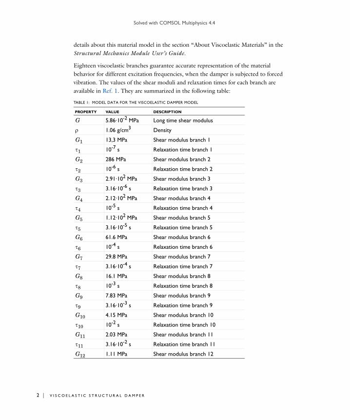
Solved with COMSOL Multiphysics 4.4
2 | V I S C
details about this material model in the section “About Viscoelastic Materials” in the Structural Mechanics Module User’s Guide.
Eighteen viscoelastic branches guarantee accurate representation of the material behavior for different excitation frequencies, when the damper is subjected to forced vibration. The values of the shear moduli and relaxation times for each branch are available in Ref. 1. They are summarized in the following table:
TABLE 1: MODEL DATA FOR THE VISCOELASTIC DAMPER MODEL
PROPERTY VALUE DESCRIPTION
G 5.86·10-2 MPa Long time shear modulus
1.06 g/cm3 Density
G1 13,3 MPa Shear modulus branch 1
1 10-7 s Relaxation time branch 1
G2 286 MPa Shear modulus branch 2
2 10-6 s Relaxation time branch 2
G3 2.91·102 MPa Shear modulus branch 3
3 3.16·10-6 s Relaxation time branch 3
G4 2.12·102 MPa Shear modulus branch 4
4 10-5 s Relaxation time branch 4
G5 1.12·102 MPa Shear modulus branch 5
5 3.16·10-5 s Relaxation time branch 5
G6 61.6 MPa Shear modulus branch 6
6 10-4 s Relaxation time branch 6
G7 29.8 MPa Shear modulus branch 7
7 3.16·10-4 s Relaxation time branch 7
G8 16.1 MPa Shear modulus branch 8
8 10-3 s Relaxation time branch 8
G9 7.83 MPa Shear modulus branch 9
9 3.16·10-3 s Relaxation time branch 9
G10 4.15 MPa Shear modulus branch 10
10 10-2 s Relaxation time branch 10
G11 2.03 MPa Shear modulus branch 11
11 3.16·10-2 s Relaxation time branch 11
G12 1.11 MPa Shear modulus branch 12
O E L A S T I C S T R U C T U R A L D A M P E R

Solved with COMSOL Multiphysics 4.4
One of the mounting elements is fixed; the other two are loaded with periodic forces with frequencies in the range 0–5 Hz.
Results and Discussion
The frequency response at 5 Hz is shown in Figure 2.
In the frequency domain, the viscoelastic properties of the material appear as the storage modulus and loss moduli. The computed variation of the viscoelastic moduli with frequency is shown in Figure 3. The result is in very good agreement with the experimental data (Figure 7 in Ref. 2)
12 0.1 s Relaxation time branch 12
G13 0.491 MPa Shear modulus branch 13
13 0.316 s Relaxation time branch 13
G14 0.326 MPa Shear modulus branch 14
14 1 s Relaxation time branch 14
G15 8.25·10-2 MPa Shear modulus branch 15
15 3.16 s Relaxation time branch 15
G16 0.126 MPa Shear modulus branch 16
16 10 s Relaxation time branch 16
G17 3.73·10-2 MPa Shear modulus branch 17
17 100 s Relaxation time branch 17
G18 1.18·10-2 MPa Shear modulus branch 18
18 1000 s Relaxation time branch 18
TABLE 1: MODEL DATA FOR THE VISCOELASTIC DAMPER MODEL
PROPERTY VALUE DESCRIPTION
3 | V I S C O E L A S T I C S T R U C T U R A L D A M P E R

Solved with COMSOL Multiphysics 4.4
4 | V I S C
.
Figure 2: Frequency response.
Figure 3: Viscoelastic storage modulus (solid line) and loss modulus (dashed line). Both quantities are normalized by 6.895 to simplify the comparison with Ref. 2.
O E L A S T I C S T R U C T U R A L D A M P E R

Solved with COMSOL Multiphysics 4.4
Notes About the COMSOL Implementation
You model in 3D and use the Solid Mechanics interface with Linear Elastic Material, add the Viscoelasticity node to the domains representing the viscoelastic layers.
References
1. S.W. Park “Analytical Modeling of Viscoelastic Dampers for Structural and Vibration Control,” Int. J. Solids and Structures, vol. 38, pp. 694–701, 2001.
2. K.L. Shen and T.T. Soong, “Modeling of Viscoelastic Dampers for Structural Applications,” J. Eng. Mech., vol. 121, pp. 694–701, 1995.
Model Library path: Structural_Mechanics_Module/Dynamics_and_Vibration/viscoelastic_damper_frequency
Modeling Instructions
From the File menu, choose New.
N E W
1 In the New window, click the Model Wizard button.
M O D E L W I Z A R D
1 In the Model Wizard window, click the 3D button.
2 In the Select Physics tree, select Structural Mechanics>Solid Mechanics (solid).
3 Click the Add button.
4 Click the Study button.
5 In the tree, select Preset Studies>Frequency Domain.
6 Click the Done button.
G E O M E T R Y 1
You import the predefined geometry from a file.
Import 11 On the Home toolbar, click Import.
2 In the Import settings window, locate the Import section.
5 | V I S C O E L A S T I C S T R U C T U R A L D A M P E R

Solved with COMSOL Multiphysics 4.4
6 | V I S C
3 Click the Browse button.
4 Browse to the model’s Model Library folder and double-click the file viscoelastic_damper.mphbin.
5 Click the Import button.
6 Click the Go to Default 3D View button on the Graphics toolbar.
The imported geometry should look similar to that shown in Figure 1.
S O L I D M E C H A N I C S
Linear Elastic Material 21 On the Physics toolbar, click Domains and choose Linear Elastic Material.
2 In the Linear Elastic Material settings window, locate the Linear Elastic Material section.
3 From the Specify list, choose Bulk modulus and shear modulus.
4 Select the Nearly incompressible material check box.
5 Select Domains 2 and 4 only.
Viscoelasticity 11 Right-click Component 1>Solid Mechanics>Linear Elastic Material 2 and choose
Viscoelasticity.
Since there are 18 branches in this material model, the data has been collected in a text file which you can load.
2 In the Viscoelasticity settings window, locate the Viscoelasticity Model section.
3 Click Load from File.
4 Browse to the model’s Model Library folder and double-click the file viscoelastic_damper_viscoelastic_data.txt.
M A T E R I A L S
On the Home toolbar, click Add Material.
A D D M A T E R I A L
1 Go to the Add Material window.
2 In the tree, select Built-In>Steel AISI 4340.
3 In the Add material window, click Add to Component.
O E L A S T I C S T R U C T U R A L D A M P E R

Solved with COMSOL Multiphysics 4.4
M A T E R I A L S
Steel AISI 43401 In the Model Builder window, under Component 1>Materials click Steel AISI 4340.
2 Select Domains 1, 3, and 5 only.
Material 21 In the Model Builder window, right-click Materials and choose New Material.
2 Right-click Material 2 and choose Rename.
3 Go to the Rename Material dialog box and type Viscoelastic in the New name edit field.
4 Click OK.
5 Select Domains 2 and 4 only.
6 In the Material settings window, locate the Material Contents section.
7 In the table, enter the following settings:
8 On the Home toolbar, click Add Material to close the Add material window.
S O L I D M E C H A N I C S
Fixed Constraint 11 On the Physics toolbar, click Boundaries and choose Fixed Constraint.
2 Select Boundaries 24–27 only.
Prescribed Displacement 11 On the Physics toolbar, click Boundaries and choose Prescribed Displacement.
2 Select Boundaries 40 and 41 only.
3 In the Prescribed Displacement settings window, locate the Prescribed Displacement section.
4 Select the Prescribed in x direction check box.
5 Select the Prescribed in y direction check box.
Property Name Value Unit Property group
Bulk modulus K 4e8 N/m² Bulk modulus and shear modulus
Shear modulus G 5.86e4 N/m² Bulk modulus and shear modulus
Density rho 1060 kg/m³ Basic
7 | V I S C O E L A S T I C S T R U C T U R A L D A M P E R

Solved with COMSOL Multiphysics 4.4
8 | V I S C
Boundary Load 11 On the Physics toolbar, click Boundaries and choose Boundary Load.
2 Select Boundaries 40 and 41 only.
3 In the Boundary Load settings window, locate the Force section.
4 Specify the FA vector as
Phase 11 Right-click Component 1>Solid Mechanics>Boundary Load 1 and choose Phase.
2 In the Phase settings window, locate the Phase section.
3 Specify the vector as
Prescribed Displacement 21 On the Physics toolbar, click Boundaries and choose Prescribed Displacement.
2 Select Boundaries 32 and 33 only.
3 In the Prescribed Displacement settings window, locate the Prescribed Displacement section.
4 Select the Prescribed in y direction check box.
Boundary Load 21 On the Physics toolbar, click Boundaries and choose Boundary Load.
2 Select Boundaries 32 and 33 only.
3 In the Boundary Load settings window, locate the Force section.
4 Specify the FA vector as
0 x
0 y
8.5e6[Pa] z
0 x
0 y
pi/2 z
5e5[Pa] x
0 y
8.5e6[Pa] z
O E L A S T I C S T R U C T U R A L D A M P E R

Solved with COMSOL Multiphysics 4.4
M E S H 1
Mesh the side surfaces of the viscoelastic layers and then sweep the resulting mesh into the layers.
Free Triangular 11 In the Model Builder window, under Component 1 right-click Mesh 1 and choose More
Operations>Free Triangular.
2 Select Boundaries 6 and 20 only.
3 Click the Build Selected button.
Swept 11 In the Model Builder window, right-click Mesh 1 and choose Swept.
2 In the Swept settings window, locate the Domain Selection section.
3 From the Geometric entity level list, choose Domain.
4 Select Domains 2 and 4 only.
Distribution 11 Right-click Component 1>Mesh 1>Swept 1 and choose Distribution.
2 In the Distribution settings window, locate the Distribution section.
3 In the Number of elements edit field, type 3.
Swept 11 Right-click Swept 1 and choose Build Selected.
Mesh the rest of the geometry using a free tetrahedral mesh.
Free Tetrahedral 12 Right-click Mesh 1 and choose More Operations>Free Tetrahedral.
9 | V I S C O E L A S T I C S T R U C T U R A L D A M P E R

Solved with COMSOL Multiphysics 4.4
10 | V I S
3 In the Model Builder window, under Component 1>Mesh 1 right-click Free Tetrahedral
1 and choose Build Selected.
The complete mesh should look similar to that shown in the figure below.
S T U D Y 1
Step 1: Frequency Domain1 In the Model Builder window, expand the Study 1 node, then click Step 1: Frequency
Domain.
2 In the Frequency Domain settings window, locate the Study Settings section.
3 In the Frequencies edit field, type range(0,0.125,0.5) range(1,0.5,5).
4 On the Study toolbar, click Show Default Solver.
R E S U L T S
Before computing the solution, set up a displacement plot that will be displayed and updated after every frequency response computation.
3D Plot Group 11 On the Home toolbar, click Add Plot Group and choose 3D Plot Group.
C O E L A S T I C S T R U C T U R A L D A M P E R

Solved with COMSOL Multiphysics 4.4
2 In the Model Builder window, under Results right-click 3D Plot Group 1 and choose Surface.
3 In the Surface settings window, click Replace Expression in the upper-right corner of the Expression section. From the menu, choose Solid
Mechanics>Displacement>Displacement field (Material)>Displacement field, Z
component (w).
4 Right-click Results>3D Plot Group 1>Surface 1 and choose Deformation.
S T U D Y 1
Step 1: Frequency Domain1 In the Model Builder window, under Study 1 click Step 1: Frequency Domain.
2 In the Frequency Domain settings window, click to expand the Results while solving section.
3 Select the Plot check box.
Solver 11 In the Model Builder window, expand the Study 1>Solver Configurations node.
2 Right-click Solver 1 and choose Compute.
R E S U L T S
3D Plot Group 11 Click the Go to Default 3D View button on the Graphics toolbar.
The computed solution should closely resemble that shown in Figure 2.
To plot the storage and loss moduli, follow these steps:
Data Sets1 On the Results toolbar, click Cut Point 3D.
2 In the Cut Point 3D settings window, locate the Point Data section.
3 In the X edit field, type 0.
4 In the Y edit field, type -0.01.
5 In the Z edit field, type 0.
1D Plot Group 21 On the Home toolbar, click Add Plot Group and choose 1D Plot Group.
2 In the 1D Plot Group settings window, locate the Data section.
3 From the Data set list, choose Cut Point 3D 1.
11 | V I S C O E L A S T I C S T R U C T U R A L D A M P E R

Solved with COMSOL Multiphysics 4.4
12 | V I S
4 Click to expand the Title section. From the Title type list, choose Manual.
5 In the Title text area, type Storage and loss moduli.
6 On the 1D Plot Group 2 toolbar, click Point Graph.
7 In the Point Graph settings window, locate the y-Axis Data section.
8 In the Expression edit field, type solid.Gstor/6.895.
9 On the 1D Plot Group 2 toolbar, click Point Graph.
10 In the Point Graph settings window, locate the y-Axis Data section.
11 In the Expression edit field, type solid.Gloss/6.895.
12 Click to expand the Coloring and style section. Find the Line style subsection. From the Line list, choose Dashed.
13 On the 1D 1D Plot Group 2 toolbar, click Plot.
C O E L A S T I C S T R U C T U R A L D A M P E R

Solved with COMSOL Multiphysics 4.4
V i s c o e l a s t i c S t r u c t u r a l Dampe r—Tran s i e n t Ana l y s i s
Introduction
The model studies the forced response of a typical viscoelastic damper. Damping elements involving layers of viscoelastic materials are often used for reduction of seismic and wind induced vibrations in buildings and other tall structures. The common feature is that the frequency of the forced vibrations is low.
Model Definition
The geometry of the viscoelastic damper is shown in Figure 1, from Ref. 1. The damper consists of two layers of viscoelastic material confined between mounting elements made of steel.
Figure 1: Viscoelastic damping element.
1 | V I S C O E L A S T I C S T R U C T U R A L D A M P E R — TR A N S I E N T A N A L Y S I S

Solved with COMSOL Multiphysics 4.4
2 | V I S C
You model the viscoelastic layers by the generalized Maxwell model available in COMSOL Multiphysics. The generalized Maxwell model represents the viscoelastic material as a series of branches, each with a spring-dashpot pair. You can find more details about this material model in the section “About Viscoelastic Materials” in the Structural Mechanics Module User’s Guide.
Eighteen viscoelastic branches guarantee accurate representation of the material behavior for different excitation frequencies, when the damper is subjected to forced vibration. The values of the shear moduli and relaxation times for each branch are available in Ref. 1. They are summarized in the following table:
TABLE 1: MODEL DATA FOR THE VISCOELASTIC DAMPER MODEL
PROPERTY VALUE DESCRIPTION
K 4·104 MPa Bulk modulus
G 5.86·10-2 MPa Long time shear modulus
1.06 g/cm3 Density
G1 13,3 MPa Shear modulus branch 1
1 10-7 s Relaxation time branch 1
G2 286 MPa Shear modulus branch 2
2 10-6 s Relaxation time branch 2
G3 2.91·102 MPa Shear modulus branch 3
3 3.16·10-6 s Relaxation time branch 3
G4 2.12·102 MPa Shear modulus branch 4
4 10-5 s Relaxation time branch 4
G5 1.12·102 MPa Shear modulus branch 5
5 3.16·10-5 s Relaxation time branch 5
G6 61.6 MPa Shear modulus branch 6
6 10-4 s Relaxation time branch 6
G7 29.8 MPa Shear modulus branch 7
7 3.16·10-4 s Relaxation time branch 7
G8 16.1 MPa Shear modulus branch 8
8 10-3 s Relaxation time branch 8
G9 7.83 MPa Shear modulus branch 9
9 3.16·10-3 s Relaxation time branch 9
G10 4.15 MPa Shear modulus branch 10
10 10-2 s Relaxation time branch 10
O E L A S T I C S T R U C T U R A L D A M P E R — TR A N S I E N T A N A L Y S I S

Solved with COMSOL Multiphysics 4.4
One of the mounting elements is fixed; the other two are loaded with periodic forces with a frequency of 3 Hz.
Results and Discussion
Figure 2 shows the results of the transient computations after one second of forced vibrations.
The typical viscoelastic hysteresis loops for a point within one of the mounting elements are shown in Figure 3.
G11 2.03 MPa Shear modulus branch 11
11 3.16·10-2 s Relaxation time branch 11
G12 1.11 MPa Shear modulus branch 12
12 0.1 s Relaxation time branch 12
G13 0.491 MPa Shear modulus branch 13
13 0.316 s Relaxation time branch 13
G14 0.326 MPa Shear modulus branch 14
14 1 s Relaxation time branch 14
G15 8.25·10-2 MPa Shear modulus branch 15
15 3.16 s Relaxation time branch 15
G16 0.126 MPa Shear modulus branch 16
16 10 s Relaxation time branch 16
G17 3.73·10-2 MPa Shear modulus branch 17
17 100 s Relaxation time branch 17
G18 1.18·10-2 MPa Shear modulus branch 18
18 1000 s Relaxation time branch 18
TABLE 1: MODEL DATA FOR THE VISCOELASTIC DAMPER MODEL
PROPERTY VALUE DESCRIPTION
3 | V I S C O E L A S T I C S T R U C T U R A L D A M P E R — TR A N S I E N T A N A L Y S I S

Solved with COMSOL Multiphysics 4.4
4 | V I S C
Figure 2: Displacement field.
Figure 3: Displacement vs. applied force.
O E L A S T I C S T R U C T U R A L D A M P E R — TR A N S I E N T A N A L Y S I S

Solved with COMSOL Multiphysics 4.4
References
1. S.W. Park “Analytical Modeling of Viscoelastic Dampers for Structural and Vibration Control,” Int. J. Solids and Structures, vol. 38, pp. 694–701, 2001.
2. K.L. Shen and T.T. Soong, “Modeling of Viscoelastic Dampers for Structural Applications,” J. Eng. Mech., vol. 121, pp. 694–701, 1995.
Model Library path: Structural_Mechanics_Module/Dynamics_and_Vibration/viscoelastic_damper_transient
Modeling Instructions
From the File menu, choose New.
N E W
1 In the New window, click the Model Wizard button.
M O D E L W I Z A R D
1 In the Model Wizard window, click the 3D button.
2 In the Select Physics tree, select Structural Mechanics>Solid Mechanics (solid).
3 Click the Add button.
4 Click the Study button.
5 In the tree, select Preset Studies>Time Dependent.
6 Click the Done button.
G E O M E T R Y 1
You import the predefined geometry from a file.
Import 11 On the Home toolbar, click Import.
2 In the Import settings window, locate the Import section.
3 Click the Browse button.
4 Browse to the model’s Model Library folder and double-click the file viscoelastic_damper.mphbin.
5 Click the Import button.
5 | V I S C O E L A S T I C S T R U C T U R A L D A M P E R — TR A N S I E N T A N A L Y S I S

Solved with COMSOL Multiphysics 4.4
6 | V I S C
6 Click the Go to Default 3D View button on the Graphics toolbar.
The imported geometry should look similar to that shown in Figure 1.
S O L I D M E C H A N I C S
Linear Elastic Material 21 On the Physics toolbar, click Domains and choose Linear Elastic Material.
2 In the Linear Elastic Material settings window, locate the Linear Elastic Material section.
3 From the Specify list, choose Bulk modulus and shear modulus.
4 Select the Nearly incompressible material check box.
5 Select Domains 2 and 4 only.
Viscoelasticity 11 Right-click Component 1>Solid Mechanics>Linear Elastic Material 2 and choose
Viscoelasticity.
Since there are 18 branches in this material model, the data has been collected in a text file which you can load.
2 In the Viscoelasticity settings window, locate the Viscoelasticity Model section.
3 Click Load from File.
4 Browse to the model’s Model Library folder and double-click the file viscoelastic_damper_viscoelastic_data.txt.
M A T E R I A L S
On the Home toolbar, click Add Material.
A D D M A T E R I A L
1 Go to the Add Material window.
2 In the tree, select Built-In>Steel AISI 4340.
3 In the Add material window, click Add to Component.
M A T E R I A L S
Steel AISI 43401 In the Model Builder window, under Component 1>Materials click Steel AISI 4340.
2 Select Domains 1, 3, and 5 only.
O E L A S T I C S T R U C T U R A L D A M P E R — TR A N S I E N T A N A L Y S I S

Solved with COMSOL Multiphysics 4.4
Material 21 In the Model Builder window, right-click Materials and choose New Material.
2 Right-click Material 2 and choose Rename.
3 Go to the Rename Material dialog box and type Viscoelastic in the New name edit field.
4 Click OK.
5 Select Domains 2 and 4 only.
6 In the Material settings window, locate the Material Contents section.
7 In the table, enter the following settings:
8 On the Home toolbar, click Add Material.
S O L I D M E C H A N I C S
Fixed Constraint 11 On the Physics toolbar, click Boundaries and choose Fixed Constraint.
2 Select Boundaries 24–27 only.
Prescribed Displacement 11 On the Physics toolbar, click Boundaries and choose Prescribed Displacement.
2 Select Boundaries 40 and 41 only.
3 In the Prescribed Displacement settings window, locate the Prescribed Displacement section.
4 Select the Prescribed in x direction check box.
5 Select the Prescribed in y direction check box.
Boundary Load 11 On the Physics toolbar, click Boundaries and choose Boundary Load.
2 Select Boundaries 40 and 41 only.
3 In the Boundary Load settings window, locate the Force section.
Property Name Value Unit Property group
Bulk modulus K 4e8 N/m² Bulk modulus and shear modulus
Shear modulus G 5.86e4 N/m² Bulk modulus and shear modulus
Density rho 1060 kg/m³ Basic
7 | V I S C O E L A S T I C S T R U C T U R A L D A M P E R — TR A N S I E N T A N A L Y S I S

Solved with COMSOL Multiphysics 4.4
8 | V I S C
4 Specify the FA vector as
Prescribed Displacement 21 On the Physics toolbar, click Boundaries and choose Prescribed Displacement.
2 Select Boundaries 32 and 33 only.
3 In the Prescribed Displacement settings window, locate the Prescribed Displacement section.
4 Select the Prescribed in y direction check box.
Boundary Load 21 On the Physics toolbar, click Boundaries and choose Boundary Load.
2 Select Boundaries 32 and 33 only.
3 In the Boundary Load settings window, locate the Force section.
4 Specify the FA vector as
D E F I N I T I O N S
Set up an integration operator to compute the total force applied to one of the mounting holes. You configure the integration to be performed on the Material frame, because this is the frame used within the Solid Mechanics interface.
Integration 11 On the Definitions toolbar, click Component Couplings and choose Integration.
2 In the Integration settings window, locate the Advanced section.
3 From the Frame list, choose Material (X, Y, Z).
4 Locate the Source Selection section. From the Geometric entity level list, choose Boundary.
5 Select Boundaries 32 and 33 only.
0 x
0 y
8.5e6[Pa]*sin(pi/2+2*pi*t*3[1/s]) z
5e5[Pa]*sin(2*pi*t*3[1/s]) x
0 y
8.5e6[Pa]*sin(2*pi*t*3[1/s]) z
O E L A S T I C S T R U C T U R A L D A M P E R — TR A N S I E N T A N A L Y S I S

Solved with COMSOL Multiphysics 4.4
Variables 11 In the Model Builder window, right-click Definitions and choose Variables.
2 In the Variables settings window, locate the Variables section.
3 In the table, enter the following settings:
M E S H 1
Mesh the side surfaces of the viscoelastic layers and then sweep the resulting mesh into the layers.
Free Triangular 11 In the Model Builder window, under Component 1 right-click Mesh 1 and choose Free
Triangular.
2 Select Boundaries 6 and 20 only.
3 Click the Build Selected button.
Swept 11 In the Model Builder window, right-click Mesh 1 and choose Swept.
2 In the Swept settings window, locate the Domain Selection section.
3 From the Geometric entity level list, choose Domain.
4 Select Domains 2 and 4 only.
Distribution 11 Right-click Component 1>Mesh 1>Swept 1 and choose Distribution.
2 In the Distribution settings window, locate the Distribution section.
3 In the Number of elements edit field, type 3.
Swept 14 Right-click Swept 1 and choose Build Selected.
Mesh the rest of the geometry using a free tetrahedral mesh.
Free Tetrahedral 11 Right-click Mesh 1 and choose Free Tetrahedral.
Name Expression Unit Description
Fz1 intop1(solid.FperAreaz)
N Total force, Z component
9 | V I S C O E L A S T I C S T R U C T U R A L D A M P E R — TR A N S I E N T A N A L Y S I S

Solved with COMSOL Multiphysics 4.4
10 | V I S
2 In the Model Builder window, under Component 1>Mesh 1 right-click Free Tetrahedral
1 and choose Build Selected.
The complete mesh should look similar to that shown in the figure below.
S T U D Y 1
Step 1: Time Dependent1 In the Model Builder window, expand the Study 1 node, then click Step 1: Time
Dependent.
2 In the Time Dependent settings window, locate the Study Settings section.
3 In the Times edit field, type range(0,0.01,1).
Solver 11 On the Study toolbar, click Show Default Solver.
2 In the Model Builder window, expand the Study 1>Solver Configurations node.
3 In the Model Builder window, expand the Solver 1 node, then click Dependent
Variables 1.
4 In the Dependent Variables settings window, locate the Scaling section.
5 From the Method list, choose Manual.
C O E L A S T I C S T R U C T U R A L D A M P E R — TR A N S I E N T A N A L Y S I S

Solved with COMSOL Multiphysics 4.4
6 In the Scale edit field, type 0.1.
This scale is applied to the visoelastic strain variables. The scales for the displacement components are chosen according to the size of the geometry. Use the following scale for the pressure help variable.
7 In the Model Builder window, under Study 1>Solver Configurations>Solver
1>Dependent Variables 1 click Auxiliary pressure (comp1.solid.pw).
8 In the Field settings window, locate the Scaling section.
9 In the Scale edit field, type 1e6.
10 In the Model Builder window, under Study 1>Solver Configurations>Solver 1 click Time-Dependent Solver 1.
11 In the Time-Dependent Solver settings window, click to expand the Output section.
12 Clear the Store time-derivatives check box.
The values of derivatives are not needed for the analysis. By not storing them, you reduce significantly the size of the output data.
R E S U L T S
Before computing the solution, set up a displacement plot that will be displayed and updated after every time step of the transient analysis.
3D Plot Group 11 On the Home toolbar, click Add Plot Group and choose 3D Plot Group.
2 In the Model Builder window, under Results right-click 3D Plot Group 1 and choose Surface.
3 In the Surface settings window, click Replace Expression in the upper-right corner of the Expression section. From the menu, choose Solid
Mechanics>Displacement>Displacement field (Material)>Displacement field, Z
component (w).
4 Right-click Results>3D Plot Group 1>Surface 1 and choose Deformation.
S T U D Y 1
Step 1: Time Dependent1 In the Model Builder window, under Study 1 click Step 1: Time Dependent.
2 In the Time Dependent settings window, click to expand the Results while solving section.
3 Locate the Results While Solving section. Select the Plot check box.
11 | V I S C O E L A S T I C S T R U C T U R A L D A M P E R — TR A N S I E N T A N A L Y S I S

Solved with COMSOL Multiphysics 4.4
12 | V I S
Solver 1In the Model Builder window, under Study 1>Solver Configurations right-click Solver 1 and choose Compute.
R E S U L T S
3D Plot Group 11 Click the Go to Default 3D View button on the Graphics toolbar.
The computed solution should closely resemble that shown in Figure 2.
1D Plot Group 21 On the Home toolbar, click Add Plot Group and choose 1D Plot Group.
2 In the 1D Plot Group settings window, click to expand the Title section.
3 From the Title type list, choose Manual.
4 In the Title text area, type Hysteresis loops.
5 On the 1D Plot Group 2 toolbar, click Point Graph.
6 Select Point 23 only.
7 In the Point Graph settings window, locate the x-Axis Data section.
8 From the Parameter list, choose Expression.
9 Click Replace Expression in the upper-right corner of the x-Axis Data section. From the menu, choose Solid Mechanics>Displacement>Displacement field
(Material)>Displacement field, Z component (w).
10 Locate the y-Axis Data section. In the Expression edit field, type Fz1.
11 On the Plot Group 2 toolbar, click Plot.
C O E L A S T I C S T R U C T U R A L D A M P E R — TR A N S I E N T A N A L Y S I S

Solved with COMSOL Multiphysics 4.4
S t r e s s R e l a x a t i o n o f a V i s c o e l a s t i c T ub e
Introduction
This model studies the temperature effects on the viscoelastic stress relaxation in a generalized Maxwell material with four branches.
Assume that the viscous part of the deformation is incompressible, so that the volume change is purely elastic. The relaxation shear modulus function is approximated by a Prony series as
(1)
where Gm represents the stiffness of the spring in the mth Maxwell branch, and m is the relaxation time of the spring-dashpot pair in the same branch.
The instantaneous shear modulus is defined as
(2)
The alternative form of Equation 1 is
(3)
where the constants m = Gm/G0 are such that
(4)
For many materials the viscoelastic properties have a strong dependence on the temperature. A common assumption is that the material is thermorheologically simple (TRS). In a material of this class, a change in the temperature can be transformed directly into a change in the time scale. Thus, the relaxation time for a TRS material is
t G Gmtm-------–
exp
m 1=
N
+=
G0 G Gm
m 1=
N
+=
t G0 0 mtm-------–
exp
m 1=
N
+=
m
m 0=
N
1=
1 | S T R E S S R E L A X A T I O N O F A V I S C O E L A S T I C TU B E

Solved with COMSOL Multiphysics 4.4
2 | S T R
modified to aTTm, where aT(T) is a shift function. One of the most commonly used shift functions is defined by the WLF (Williams-Landel-Ferry) equation:
(5)
where a base-10 logarithm is assumed. Usually T0 is the glass transition temperature of the material. Note that aT(T0) = 1. If the temperature drops below T0C2, the WLF equation is no longer valid. The constants C1 and C2 are material dependent.
Model Definition
A long thick-walled cylinder has an inner radius of 5 mm and an outer radius of 10 mm. The inner surface is subjected to a prescribed radial displacement of 0.001 mm. A four-branch generalized Maxwell model represents the viscoelastic material.
In this example, you study the decay of the stresses during a period of two hours under the influence of the temperature field. You model a quarter of the cylinder and use the Solid Mechanics interface to compute the displacements in the cylinder cross section. The geometry is shown in Figure 1.
aT logC– 1 T T0–
C2 T T0– +-----------------------------------=
E S S R E L A X A T I O N O F A V I S C O E L A S T I C TU B E
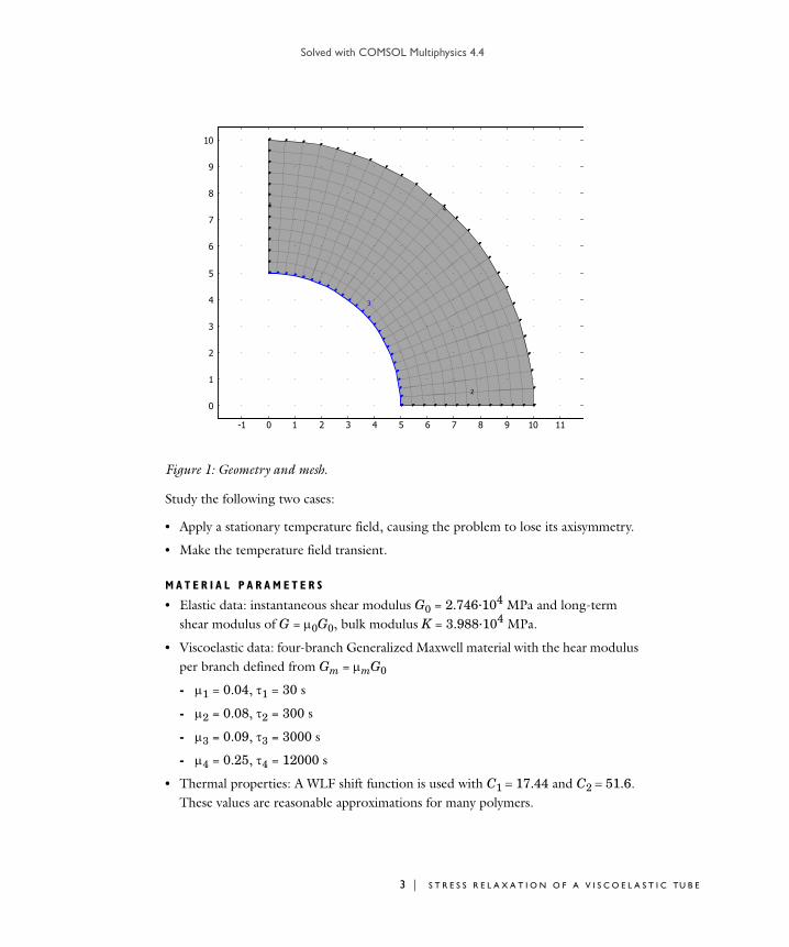
Solved with COMSOL Multiphysics 4.4
Figure 1: Geometry and mesh.
Study the following two cases:
• Apply a stationary temperature field, causing the problem to lose its axisymmetry.
• Make the temperature field transient.
M A T E R I A L P A R A M E T E R S
• Elastic data: instantaneous shear modulus G0 = 2.746·104 MPa and long-term shear modulus of G = 0G0, bulk modulus K = 3.988·104 MPa.
• Viscoelastic data: four-branch Generalized Maxwell material with the hear modulus per branch defined from Gm = mG0
- 1 = 0.04, 1 = 30 s
- 2 = 0.08, 2 = 300 s
- 3 = 0.09, 3 = 3000 s
- 4 = 0.25, 4 = 12000 s
• Thermal properties: A WLF shift function is used with C117.44 and C251.6. These values are reasonable approximations for many polymers.
3 | S T R E S S R E L A X A T I O N O F A V I S C O E L A S T I C TU B E

Solved with COMSOL Multiphysics 4.4
4 | S T R
• The reference temperature is 500 K.
• Heat transfer properties: 7850 kg/m37.85·109 t/mm3, Cp = 2100 J/(kg·K) = 2100·106 N·mm/(t·K), k = 6·102 W/(m·K) = 6·102 N/(s·K).
C O N S T R A I N T S
• The circumferential displacements are constrained on the radial edges.
• The inner edge of the hole is constrained to a radial displacement of 0.001 mm.
H E A T TR A N S F E R B O U N D A R Y C O N D I T I O N S
• Stationary analysis: The inner and outer circular edges both have a temperature distribution varying linearly with the y-coordinate from 500 K at the y = 0 symmetry section to 506 K at the x = 0 symmetry section.
• Transient analysis: The temperature distribution obtained from the stationary analysis is used as initial condition, while all edges are insulated.
Results and Discussion
In the first case, the temperature field is stationary and is shown in Figure 2.
Figure 2: Stationary temperature distribution.
E S S R E L A X A T I O N O F A V I S C O E L A S T I C TU B E

Solved with COMSOL Multiphysics 4.4
The stress relaxation is faster where the temperature is higher. In Figure 3, the plots of radial stresses at radius 7.5 mm display this effect. The solid line is taken at y = 0 (cold) and the dashed line at x = 0 (warm).
Figure 3: Stress relaxation under a stationary temperature distribution.
In the second case, the temperature initially has the same distribution as shown in Figure 2, but it is allowed to settle in time to a final homogeneous value. Again, compare the radial stresses at radius 7.5 mm. The initial behavior is similar to the previous case, but as the difference in material properties decreases, the curves approach each other; see Figure 4. The strain rate in the initially warm point decreases, while it increases in the initially cold point.
5 | S T R E S S R E L A X A T I O N O F A V I S C O E L A S T I C TU B E
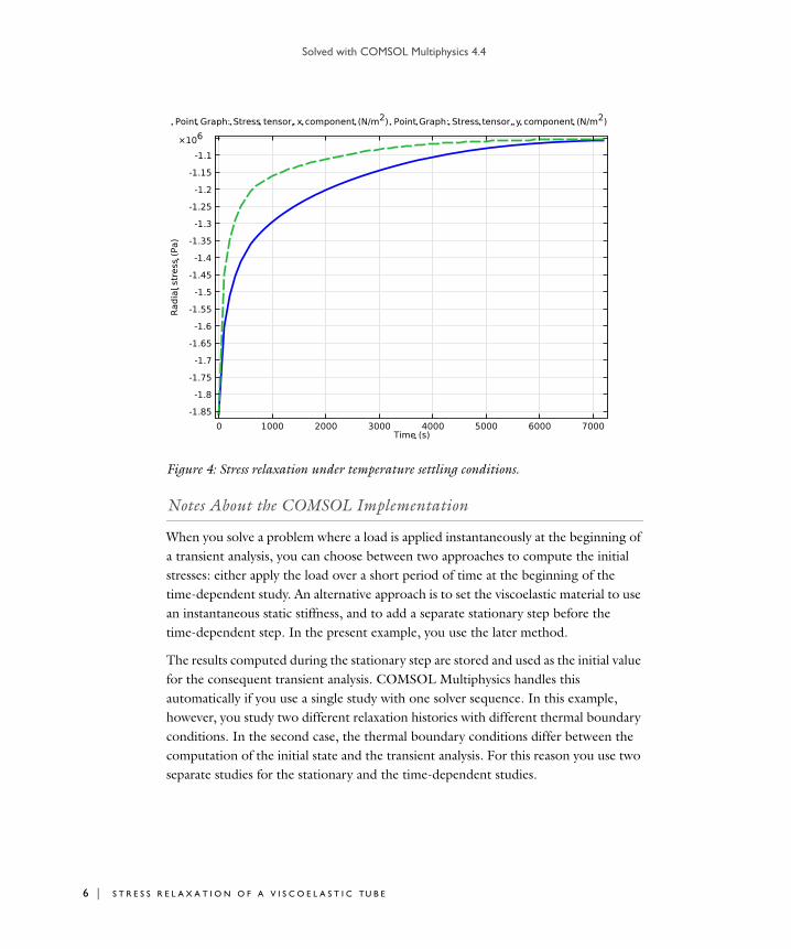
Solved with COMSOL Multiphysics 4.4
6 | S T R
Figure 4: Stress relaxation under temperature settling conditions.
Notes About the COMSOL Implementation
When you solve a problem where a load is applied instantaneously at the beginning of a transient analysis, you can choose between two approaches to compute the initial stresses: either apply the load over a short period of time at the beginning of the time-dependent study. An alternative approach is to set the viscoelastic material to use an instantaneous static stiffness, and to add a separate stationary step before the time-dependent step. In the present example, you use the later method.
The results computed during the stationary step are stored and used as the initial value for the consequent transient analysis. COMSOL Multiphysics handles this automatically if you use a single study with one solver sequence. In this example, however, you study two different relaxation histories with different thermal boundary conditions. In the second case, the thermal boundary conditions differ between the computation of the initial state and the transient analysis. For this reason you use two separate studies for the stationary and the time-dependent studies.
E S S R E L A X A T I O N O F A V I S C O E L A S T I C TU B E

Solved with COMSOL Multiphysics 4.4
Model Library path: Structural_Mechanics_Module/Viscoelasticity/viscoelastic_tube
Modeling Instructions
From the File menu, choose New.
N E W
1 In the New window, click the Model Wizard button.
M O D E L W I Z A R D
1 In the Model Wizard window, click the 2D button.
2 In the Select Physics tree, select Structural Mechanics>Solid Mechanics.
3 Click the Add button.
4 In the Select Physics tree, select Heat Transfer>Heat Transfer in Solids.
5 Click the Add button.
6 Click the Done button.
G E O M E T R Y 1
1 In the Model Builder window, under Component 1 click Geometry 1.
2 In the Geometry settings window, locate the Units section.
3 From the Length unit list, choose mm.
Circle 1 1 Right-click Component 1 >Geometry 1 and choose Circle.
2 In the Circle settings window, locate the Size and Shape section.
3 In the Radius edit field, type 10.
4 Click the Build Selected button.
Circle 2 1 In the Model Builder window, right-click Geometry 1 and choose Circle.
2 In the Circle settings window, locate the Size and Shape section.
3 In the Radius edit field, type 5.
4 Click the Build Selected button.
7 | S T R E S S R E L A X A T I O N O F A V I S C O E L A S T I C TU B E

Solved with COMSOL Multiphysics 4.4
8 | S T R
Difference 1 1 On the Geometry toolbar, click Difference.
2 Select the object c1 only.
3 In the Difference settings window, locate the Difference section.
4 Select the Objects to subtract toggle button.
5 Select the object c2 only.
6 Click the Build Selected button.
Rectangle 1 1 Right-click Geometry 1 and choose Rectangle.
2 In the Rectangle settings window, locate the Size section.
3 In the Width edit field, type 11.
4 In the Height edit field, type 11.
5 Click the Build Selected button.
Intersection 11 On the Geometry toolbar, click Intersection.
2 Select the objects r1 and dif1 only.
3 Click the Build Selected button.
4 Click the Zoom Extents button on the Graphics toolbar.
Form Union 1 In the Model Builder window, under Component 1>Geometry 1 right-click Form Union
(fin) and choose Build Selected.
The equations only need to include first-order time derivatives since inertial effects can be neglected for this class of problems.
S O L I D M E C H A N I C S
1 In the Model Builder window, under Component 1 click Solid Mechanics.
2 In the Solid Mechanics settings window, locate the Structural Transient Behavior section.
3 From the list, choose Quasi-static.
Linear Elastic Material 11 In the Model Builder window, under Component 1 >Solid Mechanics click Linear Elastic
Material 1.
E S S R E L A X A T I O N O F A V I S C O E L A S T I C TU B E

Solved with COMSOL Multiphysics 4.4
2 In the Linear Elastic Material settings window, locate the Linear Elastic Material section.
3 From the Specify list, choose Bulk modulus and shear modulus.
Viscoelasticity 11 Right-click Component 1 >Solid Mechanics>Linear Elastic Material 1 and choose
Viscoelasticity.
2 In the Viscoelasticity settings window, locate the Viscoelasticity Model section.
3 In the table, modify the settings to:
4 Click Add.
5 In the table, modify the settings to:
6 Click Add.
7 In the table, modify the settings to:
8 Click Add.
9 In the table, modify the settings to:
10 Locate the Model Inputs section. From the T list, choose Temperature.
11 Locate the Thermal Effects section. From the Shift function list, choose Williams-Landel-Ferry.
12 In the TWLF edit field, type 500[K].
13 Locate the Viscoelasticity Model section. From the Static stiffness list, choose Instantaneous.
Branch Shear modulus (Pa) Relaxation time (s)
1 0.04*G_inst 30
Branch Shear modulus (Pa) Relaxation time (s)
1 0.08*G_inst 300
Branch Shear modulus (Pa) Relaxation time (s)
1 0.09*G_inst 3000
Branch Shear modulus (Pa) Relaxation time (s)
1 0.25*G_inst 12000
9 | S T R E S S R E L A X A T I O N O F A V I S C O E L A S T I C TU B E

Solved with COMSOL Multiphysics 4.4
10 | S T
Symmetry 11 On the Physics toolbar, click Boundaries and choose Symmetry.
2 Select Boundaries 1 and 2 only.
Prescribed Displacement 11 On the Physics toolbar, click Boundaries and choose Prescribed Displacement.
2 Select Boundary 3 only.
3 In the Prescribed Displacement settings window, locate the Coordinate System
Selection section.
4 From the Coordinate system list, choose Boundary System 1 (sys1).
5 Locate the Prescribed Displacement section. Select the Prescribed in n direction check box.
6 In the u0n edit field, type -1e-6.
H E A T TR A N S F E R I N S O L I D S
Temperature 11 On the Physics toolbar, click Boundaries and choose Temperature.
2 Select Boundaries 3 and 4 only.
3 In the Temperature settings window, locate the Temperature section.
4 In the T0 edit field, type (500+6*y/sqrt(x^2+y^2))[K].
M A T E R I A L S
Material 1 (mat1)1 In the Model Builder window, under Component 1 right-click Materials and choose
New Material.
2 Select Domain 1 only.
3 In the Material settings window, locate the Material Contents section.
4 In the table, enter the following settings:
Property Name Value Unit Property group
Bulk modulus K 3.988e4[MPa] N/m² Bulk modulus and shear modulus
Shear modulus G 0.54*G_inst N/m² Bulk modulus and shear modulus
Density rho 7.85E-9[t/mm^3] kg/m³ Basic
R E S S R E L A X A T I O N O F A V I S C O E L A S T I C TU B E

Solved with COMSOL Multiphysics 4.4
D E F I N I T I O N S
Variables 11 In the Model Builder window, under Component 1 right-click Definitions and choose
Variables.
2 In the Variables settings window, locate the Variables section.
3 In the table, enter the following settings:
M E S H 1
Mapped 1In the Model Builder window, under Component 1 right-click Mesh 1 and choose Mapped.
Distribution 11 In the Model Builder window, under Component 1 >Mesh 1 right-click Mapped 1 and
choose Distribution.
2 Select Boundary 1 only.
3 In the Distribution settings window, locate the Distribution section.
4 In the Number of elements edit field, type 12.
Distribution 21 Right-click Mapped 1 and choose Distribution.
2 Select Boundary 3 only.
3 In the Distribution settings window, locate the Distribution section.
4 In the Number of elements edit field, type 24.
5 Click the Build All button.
6 Click the Zoom Extents button on the Graphics toolbar.
Thermal conductivity
k 0.06[N/(s*K)] W/(m·K) Basic
Heat capacity at constant pressure
Cp 2.1E9[N*mm/(t*K)] J/(kg·K) Basic
Name Expression Unit Description
G_inst 2.746e4[MPa] Pa Instantaneous shear modulus
Property Name Value Unit Property group
11 | S T R E S S R E L A X A T I O N O F A V I S C O E L A S T I C TU B E

Solved with COMSOL Multiphysics 4.4
12 | S T
R O O T
Next, add a stationary study to model the instantaneous preloading step.
On the Home toolbar, click Add Study.
A D D S T U D Y
1 Go to the Add Study window.
2 Find the Studies subsection. In the tree, select Preset Studies>Stationary.
3 In the Add Study window, click Add Study.
4 On the Home toolbar, click Add Study to close the Add Study window.
S T U D Y 1
On the Home toolbar, click Compute.
R E S U L T S
Display the stationary temperature.
Temperature (ht)1 On the Temperature (ht) toolbar, click Plot.
2 Click the Zoom Extents button on the Graphics toolbar.
Proceed to add a transient study for analyzing the stress relaxation process.
On the Home toolbar, click Add Study.
A D D S T U D Y
1 Go to the Add Study window.
2 Find the Studies subsection. In the tree, select Preset Studies>Time Dependent.
3 In the Add Study window, click Add Study.
4 On the Home toolbar, click Add Study to close the Add Study window.
S T U D Y 2
Step 1: Time Dependent1 In the Model Builder window, under Study 2 click Step 1: Time Dependent.
2 In the Time Dependent settings window, locate the Study Settings section.
3 In the Times edit field, type range(0,100,7200).
4 Select the Relative tolerance check box.
5 In the associated edit field, type 1e-3.
R E S S R E L A X A T I O N O F A V I S C O E L A S T I C TU B E

Solved with COMSOL Multiphysics 4.4
Solver 21 On the Study toolbar, click Show Default Solver.
2 In the Model Builder window, expand the Study 2>Solver Configurations node.
3 In the Model Builder window, expand the Solver 2 node, then click Dependent
Variables 1.
4 In the Dependent Variables settings window, locate the General section.
5 From the Defined by study step list, choose User defined.
6 Locate the Initial Values of Variables Solved For section. From the Method list, choose Solution.
7 From the Solution list, choose Solver 1.
8 Locate the Scaling section. From the Method list, choose Initial value based.
9 In the Model Builder window, under Study 2>Solver Configurations>Solver 2 click Time-Dependent Solver 1.
10 In the Time-Dependent Solver settings window, click to expand the Absolute tolerance section.
11 In the Tolerance edit field, type 0.0001.
12 Click to expand the Time stepping section.
13 From the Steps taken by solver list, choose Intermediate.
14 Click to collapse the Time Stepping section. In the Model Builder window, under Study
2>Solver Configurations>Solver 2 click Dependent Variables 1.
15 In the Dependent Variables settings window, locate the Scaling section.
16 From the Method list, choose Manual.
17 In the Scale edit field, type 1e-5.
This scale is applied to the viscoelastic strain variables. The scales for the displacement components are chosen according to the size of the geometry. Use the following scale for the temperature.
18 In the Model Builder window, under Study 2>Solver Configurations>Solver
2>Dependent Variables 1 click Temperature (comp1.T).
19 In the Field settings window, locate the Scaling section.
20 From the Method list, choose Manual.
21 In the Scale edit field, type 500.
22 On the Home toolbar, click Compute.
13 | S T R E S S R E L A X A T I O N O F A V I S C O E L A S T I C TU B E

Solved with COMSOL Multiphysics 4.4
14 | S T
R E S U L T S
Temperature 11 Click the Zoom Extents button on the Graphics toolbar.
Compare the temperature distribution at the end of the simulation interval with the stationary temperature distribution shown in Figure 2.
Next, set up the stress relaxation plot shown in Figure 3.
Data Sets1 On the Results toolbar, click Cut Point 2D.
2 In the Cut Point 2D settings window, locate the Point Data section.
3 In the X edit field, type 7.5.
4 In the Y edit field, type 0.
5 Locate the Data section. From the Data set list, choose Solution 2.
6 On the Results toolbar, click Cut Point 2D.
7 In the Cut Point 2D settings window, locate the Point Data section.
8 In the X edit field, type 0.
9 In the Y edit field, type 7.5.
10 Locate the Data section. From the Data set list, choose Solution 2.
1D Plot Group 71 On the Home toolbar, click Add Plot Group and choose 1D Plot Group.
2 In the 1D Plot Group settings window, locate the Data section.
3 From the Data set list, choose Solution 2.
4 On the 1D Plot Group 7 toolbar, click Point Graph.
5 In the Point Graph settings window, locate the Data section.
6 From the Data set list, choose Cut Point 2D 1.
7 Locate the y-Axis Data section and type solid.sx. On the 1D Plot Group 7 toolbar, click Plot.
8 On the 1D Plot Group 7 toolbar, click Point Graph.
9 In the Point Graph settings window, locate the Data section.
10 From the Data set list, choose Cut Point 2D 2.
11 Locate the y-Axis Data section and type solid.sy. On the 1D Plot Group 7 toolbar, click Plot.
R E S S R E L A X A T I O N O F A V I S C O E L A S T I C TU B E

Solved with COMSOL Multiphysics 4.4
12 Click to expand the Coloring and style section. Locate the Coloring and Style section. Find the Line style subsection. In the Width edit field, type 2.
13 From the Line list, choose Dashed.
14 In the Model Builder window, under Results>1D Plot Group 7 click Point Graph 1.
15 In the Point Graph settings window, locate the Coloring and Style section.
16 Find the Line style subsection. In the Width edit field, type 2.
17 In the Model Builder window, click 1D Plot Group 7.
18 In the 1D Plot Group settings window, locate the Plot Settings section.
19 Select the x-axis label check box.
20 In the associated edit field, type Time (s).
21 Select the y-axis label check box.
22 In the associated edit field, type Radial stress (Pa).
S T U D Y 2
Step 1: Time Dependent1 In the Model Builder window, under Study 2 click Step 1: Time Dependent.
2 In the Time Dependent settings window, locate the Physics and Variables Selection section.
3 Select the Modify physics tree and variables for study step check box.
4 In the Physics and variables selection tree, select Component 1 >Heat Transfer in Solids
>Temperature 1.
5 Click Disable.
6 On the Home toolbar, click Compute.
R E S U L T S
1D Plot Group 71 On the 1D Plot Group 7 toolbar, click Plot.
Compare the resulting plot with that in Figure 4.
15 | S T R E S S R E L A X A T I O N O F A V I S C O E L A S T I C TU B E

Solved with COMSOL Multiphysics 4.4
16 | S T
R E S S R E L A X A T I O N O F A V I S C O E L A S T I C TU B E


