4 Trigonometry and Complex · PDF file4 Trigonometry and Complex Numbers ... When any operation is applied to an angle represented in degrees by a mathematics superscript, such as

4 Trigonometry and ComplexNumbers

Trigonometry developed from the study of triangles, particularly right triangles, and therelations between the lengths of their sides and the sizes of their angles. The trigono-metric functions that measure the relationships between the sides of similar triangleshave far-reaching applications that extend far beyond their use in the study of triangles.Complex numbers were developed, in part, because they complete, in a useful and ele-gant fashion, the study of the solutions of polynomial equations. Complex numbers areuseful not only in mathematics, but in the other sciences as well.

Trigonometry

Most of the trigonometric computations in this chapter use six basic trigonometric func-tions The two fundamental trigonometric functions, sine and cosine, can be de¿ned interms of the unit circle—the set of points in the Euclidean plane of distance one fromthe origin. A point on this circle has coordinates+frv w> vlq w,, wherew is a measure (inradians) of the angle at the origin between the positive{-axis and the ray from the ori-gin through the point measured in the counterclockwise direction. The other four basictrigonometric functions can be de¿ned in terms of these two—namely,

wdq{ @vlq{

frv{vhf{ @

4

frv{

frw{ @frv{

vlq{fvf{ @

4

vlq{

For3 ? w ?�

5, these functions can be found as a ratio of certain sides of a right triangle

that has one angle of radian measurew.

Trigonometric Functions

The symbols used for the six basic trigonometric functions—vlq, frv, wdq, frw, vhf,fvf—are abbreviations for the words cosine, sine, tangent, cotangent, secant, and cose-cant, respectively.You can enter these trigonometric functions and many other functionseither from the keyboard in mathematics mode or from the dialog box that drops down

when you click or chooseInsert + Math Name. When you enter one of thesefunctions from the keyboard in mathematics mode, the function name automatricallyturns gray when you type the¿nal letter of the name.

90 Chapter 4 Trigonometry and Complex Numbers

Note Ordinary functions require parentheses around the function argument, whiletrigonometric functions commonly do not. The default behavior of your system allowstrigonometric functions without parentheses. If you want parentheses to be required forall functions, you can change this behavior in the Maple Settings dialog. Click the Def-inition Options tab and under Function Argument Selection Method, check ConvertTrigtype to Ordinary. For further information see page 126.

To ¿nd values of the trigonometric functions, use Evaluate or Evaluate Numeri-cally.

L Evaluate

vlq 6�7 @ 4

5

s5 vlq +4, @ vlq 4 vlq 93� @ 4

5

s6

L Evaluate Numerically

vlq 6�7 @ = :3:44 vlq +4, @ = ;747: vlq 93� @ = ;9936

The notation you use determines whether the argument is interpreted as radians ordegrees: vlq 63 @ �=<;;36 and vlq 63� @ =8. The degree symbol can be either asmall green or red circle. The small green circle is entered from the Insert + UnitName dialog. The small red circle appears on the Common Symbols toolbar and onthe Binary Operations symbol panel, and must be entered as a superscript. With nosymbol, the argument is interpreted as radians, and with either a green or red degreesymbol, the argument is interpreted as degrees.

All operations will convert angle measure to radians. See page 91 for a discussion ofconversion. See page 37 for a discussion of units that can be used for plane angles.

Your choice for Digits Used in Display in the Maple + Settings dialog determinesthe number of places displayed in the response to Evaluate Numerically.

Expression Evaluate Evaluate Numericallyvlq �

745

s5 =:3:44

vlq 47�6:3 vlq;::

43;33� =58568

orj43 vlq{oq +vlq{,

oq 5 . oq 8=7675< oq +vlq{,

6�87346

933� 9=;39;� 43�5

Solving Trigonometric Equations

You can use both Exact and Numeric from the Solve submenu to ¿nd solutions totrigonometric equations. These operations also convert degrees to radians. Use of deci-mal notation in the equation gives you a numerical solution, even withExact.

Trigonometry 91

Equation Solve + Exact Solve + Numeric{ @ vlq �

7 { @ 45

s5 { @ =:3:44

vlq 55� @47

ff @

47

vlq 44<3�

f @ 6:=6:6

orj43 vlq{ @ �4=49:< { @ 9=:<;;� 43�5 { @ 6=3:69

{ @ 6�873 { @ 46933� { @ 9=;39;� 43�5

Note that the answers are different for the equation orj43 vlq{ @ �4=49:<. This dif-ference occurs because there are multiple solutions and the two commands are¿ndingdifferent solutions. TheNumeric command from theSolve submenu offers the ad-vantage that you can specify a range in which you wish the solution to lie. Enter theequation and the range in different rows of a display or a one-column matrix.

L Solve + Numeric

{ @ 43 vlq{{ 5 +8>4,

, Solution is:i{ @ :=39;5j

The interval+8>4, was speci¿ed for the solution in the preceding example. Byspecifying other intervals, you can¿nd all seven solutions:i{ @ 3j, i{ @ 5=;856j,i{ @ :=39;5j, i{ @ ;=7565j, as depicted in the following graph. TheExact com-mand for solving equations gives only the solution{ @ 3 for this equation.

-10

-5

0

5

10

-10 -5 5 10x

When any operation is applied to an angle represented in degrees by a mathematicssuperscript, such as7;�, degrees are automatically converted to radians. To go in theother direction, replace5� radians with693� and convert other angles proportionately.You can also solve directly for the number of degrees. Both methods follow.

L To convert radians to degrees (using ratios)

1. Write the equation�

693@

{

5�, where{ represents radians.

2. Leave the insertion point in this equation.

3. From theSolve submenu, chooseExact or Numeric.


4. Name � as the Variable to Solve for.

5. Choose OK to get � @4;3

�{.

L To convert radians to degrees (directly)

1. Write an equation such as 5 @ ��, or (using Insert + Unit Name) 5 udg @ � �.


3. From the Solve submenu, choose Exact or Numeric, to get � @ 693� or � @ 447= 8<

Example 17 Convert { @46

933� radians to degrees as follows.

1. Write the equation�

693@

�46933�

�5�

.


3. From the Solve submenu, choose Exact to get � @ 6<43 degrees, or choose Numeric

to get � @ 6=< degrees=

- or -

1. Write the equation46

933� @ ��

2. Leave the insertion point in this equation

3. From theSolve submenu, chooseExact to get� @ 6<43 , or chooseNumeric to get

� @ 6=<.

See page 43 for additional examples of converting units.

L To change 3=< degrees to minutes

� Apply Evaluate to3=<� 93

to get3=<� 93 @ 87=3

- or -

� Enter degree and minute symbols from the Unit Name dialog. ApplySolve to3=< � @ { 3

to get{ @ 87=3

Trigonometry 93

To check these results, apply Evaluate to 6�873 or 6 � 87 3 to get

6�873 @46

933� or 6 � 87 3 @ 9= ;39 ;� 43�5 udg

Trigonometric Identities

This section illustrates the effects of some operations on trigonometric functions. First,simpli¿cations and expansions of various trigonometric expressions illustrate many ofthe familiar trigonometric identities.

De¿nitions in Terms of Basic Trigonometric FunctionsApply Simplify to the secant, and cosecant to ¿nd their de¿nition in terms of the sineand cosine functions.

L Simplify

vhf{ @4

frv{fvf{ @

4

vlq{

Pythagorean Identities

L Simplify

vlq5 {. frv5 { @ 4 wdq5 {� vhf5 { @ �4 frw5 {� fvf5 { @ �4

Addition Formulas

L Expand

vlq +{. |, @ vlq{ frv | . frv{ vlq | frv +{. |, @ frv{ frv | � vlq{ vlq |

wdq +{. |, @wdq{. wdq|

4� wdq{ wdq |

Apply Combine + Trig Functions to the expansions of vlq +{. |, and frv +{. |,to return them to their original form and to change the expansion of wdq +{. |, to theform vlq+{.|,

frv+{.|, .


Double-Angle Formulas

L Expand

vlq 5� @ 5 vlq � frv � frv 5� @ 5frv5 � � 4

wdq 5� @ 5 +vlq �,frv �

5 frv5 � � 4

You can uncover other multiple-angle formulas withExpand. Following are someexamples.

L Expand

vlq 9� @ 65 vlq � frv8 � � 65 vlq � frv6 � . 9 vlq � frv �

vlq 57� @ ;6;;93; vlq � frv56 � � 7946:677 vlq � frv54 �

.4434337;3 vlq � frv4< � � 47<7553;3 vlq � frv4: �

.45:33;:9; vlq � frv48 � � :34;<389 vlq � frv46 �

.5867937; vlq � frv44 � � 8;8:5;3 vlq � frv< �

.;569;3 vlq � frv: � � 97397 vlq � frv8 �

.55;; vlq � frv6 � � 57 vlq � frv �

vlq+5d. 6e, @ ; vlqd frv d frv6 e � 9 vlqd frvd frv e

. ; frv5 d vlq e frv5 e � 5 frv5 d vlq e

� 7 vlq e frv5 e . vlq e

Combining and Simplifying Trigonometric Expressions

Products and powers of trigonometric functions and hyperbolic functions are combinedinto a sum of trigonometric functions or hyperbolic functions whose arguments are in-tegral linear combinations of the original arguments.

L Combine + Trig Functions

vlq{ vlq | @ 45 frv +{� |,� 4

5 frv +{. |, vlq5 { @ 45 � 4

5 frv 5{

vlq{ frv | @ 45 vlq +{. |, . 4

5 vlq +{� |, frv5 { @ 45 frv 5{. 4

5

vlq8 { frv8 { @ 4845 vlq 43{. 8

589 vlq 5{� 8845 vlq 9{

vlqk6 { frvk6 { @ 465 vlqk 9{� 6

65 vlqk 5{ vlqk{ frvk{ @ 45 vlqk 5{

The commandSimplify combines and simpli¿es trigonometric expressions, as in the

Trigonometry 95

following examples.

L Simplify

frv5 {. 47 vlq

5 5{� vlq5 { frv5 {. 5 vlq5 { @ � frv5 {. 5

+frv 6w. 6frv w, vhf w @ 7 frv5 w vlq 6d. 7 vlq6 d @ 6 vlqd

wdq �5 vlq

�5 . frv �5 � 5 fvf � vlq �

5 @ 3

You may need to apply repeated operations to get the result you want. The orderin which you apply the operations is not necessarily critical. You achieve the ¿rst ofthe following examples by applying Simplify followed by Expand. For the secondexample, apply Expand followed by Simplify.

L Simplify, Expand

+vhf w, +4 . frv 5w, @4

frv w+4 . frv 5w, @ 5 frv w

L Expand, Simplify

+vhf w, +4 . frv 5w, @ 5 vhf w frv5 w @ 5 frv w

Solution of Triangles

To solve a triangle means to determine the lengths of the three sides and the measures(in degrees or radians) of the three angles.

Solving a Right TriangleYou can solve a right triangle with sides d> e> f and opposite angles �> �> �, respectively,if you know the value of one side and one acute angle, or the value of any two sides.

Example 18 To solve the right triangle with one side of length f @ 5 and one angle� @ �

< ,

1. Choose New De¿nition from the De¿ne menu for each of the given values � @ �<

and f @ 5.

2. Apply Evaluate to � @ �5 � � to get � @ :

4;�.

3. Apply Evaluate (or Evaluate Numerically) to d @ f vlq� to get d @ 5 vlq 4<�

+@ =9;737,.

4. Apply Evaluate to e @ f frv� to get e @ 5frv 4<� +@ 4=;:<7,.

Example 19 To solve a right triangle given two sides, say d @ 4< and f @ 56,


1. Apply De¿ne to each of the given values, d @ 4< and f @ 56.

2. Place the insertion point in the equation d5 . e5 @ f5.

3. From the Solve submenu, choose Exact to get e @ 5s75.

4. Place the insertion point in each of the equations vlq� @d

f, frv� @

d

fin turn.

5. From the Solve submenu, choose Exact to get � @ dufvlq 4<56 , � @ duffrv 4<

56 =

For a numerical result, evaluate these functions numerically, or choose Numericrather than Exact from the Solve submenu in the ¿nal step. You need to specify intervals

for � and �, such as�

vlq� @ d@f� 5 +3> �@5,

�and

�frv� @ d@f� 5 +3> �@5,

�, before applying Solve +

Numeric or you may get a solution greater than �5 . Specifying these intervals gives the

solutione @ 45=<9> � @ =<:54 > � @ =8<;:

Solving General TrianglesThe law of sines

d

vlq�@

e

vlq�@

f

vlq�enables you to solve a triangle if you are given one side and two angles, or if you aregiven two sides and an angle opposite one of these sides.

a

b

cβ

α

γ

Example 20 To solve a triangle given one side and two angles,

1. Use New De¿nition on the De¿ne submenu to de¿ne � @ �< , � @ 5�

< , and f @ 5

2. Evaluate � @ � � �� to get � @ 56�.

3. Use New De¿nition on the De¿ne submenu to de¿ne � @ 56�.

4. Apply Solve + Exact tod

vlq�@

f

vlq�and to

e

vlq�@

f

vlq�to get

d @7

6

s6 vlq

4

<� and e @

7

6

s6 vlq

5

<�

Trigonometry 97

You can apply Solve + Numeric to get numerical solutions, or you can evaluate thepreceding solutions numerically.

Using both the law of sines and the law of cosines,

d5 . e5 � 5de frv � @ f5

you can solve a triangle given two sides and the included angle, or given three sides.

Example 21 To solve a triangle given two sides and the included angle,

1. De¿ne each of d @ 5=67, e @ 6=8:, and � @ 5<549�.

2. Apply Solve + Exact to d5 . e5 � 5de frv� @ f5 to get f @ 4=:588.

3. De¿ne f @ 4=:588.

4. Apply Solve + Exact to bothd

vlq�@

f

vlq�and

e

vlq�@

f

vlq�to get � @ =8;;8<

and � @ 4=3437.

A triangle with three sides given is solved similarly: interchange the actions on �and f in the steps just described.

Example 22 To solve a triangle given three sides,

1. De¿ne d @ 5=86, e @ 7=48, and f @ 9=4<.

2. Apply Solve + Exact to d5 . e5 � 5de frv� @ f5 to get � @ 5=678;.

3. De¿ne � @ 5=678;.

4. Apply Solve + Exact tod

vlq�@

f

vlq�to get � @ =5<965, and to

e

vlq�@

f

vlq�to

get � @ =7<<7;.

Inverse Trigonometric Functions and TrigonometricEquations

The following type of question arises frequently when working with the trigonometricfunctions: for which angles { is vlq{ @ |? There are many correct answers to thesequestions, since the trigonometric functions are periodic. The inverse trigonometricfunctions provide answers to such questions that lie within a restricted domain. Theinverse sine function, for example, produces the angle { between ��

5 and �5 that satis¿es

vlq{ @ |. This solution is denoted by dufvlq{ or vlq�4 {.The inverse trigonometric functions and a number of other functions are available

in the dialog box that comes up when you click the Math Name button on the Mathtoolbar. They can also be entered from the keyboard in mathematics mode.

Example 23 To ¿nd the angle { (between ��5 and �

5 ) for which wdq{ @ 433,


� Leave the insertion point in the expression dufwdq 433=

� Apply Evaluate Numerically

This gives dufwdq 433 @ 4=893:<999

You can also ¿nd an angle satisfying wdq{ @ 433 by applying Solve + Numeric tothe equation. This technique does not necessarily ¿nd the solution between ��

5 and �5 .

In this case, in fact, it gives the solution { @ 435=3<4:9, which is 4=893:<999 . 65�.You can specify the interval for the solution, as follows.

L Solve + Numeric

wdq{ @ 433{ 5 ��

5 >�5

� , Solution is : i{ @ 4=893:<999j

Using this technique, you can ¿nd solutions to a variety of trigonometric equationsin speci¿ed intervals. Following are some examples of equations that you can solve withSolve + Exact and Solve + Numeric.

Equation Solve + Exact Solve + Numericvlq w @ vlq 5w iw @ 3j > �w @ 4

6��

w @ 8=569; wdq{� 46 . 8 wdq5 { @ 6 { @ dufwdq

��78 7

8

s9�

{ @ �5=5;57

wdq5 {� frw5 { @ 4 { @ dufvlq�45

s�5 5

s8�

{ @ 5=56:

Note that Solve + Exact gives multiple solutions in these examples, whereas Solve+ Numeric returns only one solution. In general, applying Evaluate Numerically tothe exact solutions gives numerical solutions different from those produced by Solve+ Numeric. This is a good place to experiment with a plot to visualize the completesolution. You can see in the following plot, for example, the pattern of crossings ofthe graphs of | @ wdq5 { � frw5 { and | @ 4, depicting the solutions of the equationwdq5 {� frw5 { @ 4.

-10

-5

0

5

10

-8 -6 -4 -2 2 4 6 8x

| @ wdq5 {� frw5 {, | @ 4

Solutions can be found in a speci¿ed range with Solve + Numeric, as demonstrated

Complex Numbers 99

in the following example. Enter the equation and the range in different rows of a one-column matrix.

L Solve + Numeric

; wdq{� 46 . 8 wdq5 { @ 6{ 5 ��

5 >�5

� , Solution is :i{ @ =;8<49j

Complex Numbers

For a review of the arithmetic of complex numbers, see page 32.

DeMoivre’s Theorem

Any pair +d> e, of real numbers can be represented in polar coordinates with d @ u frv �and e @ u vlq � where u @

sd5 . e5 is the distance from the point +d> e, to the origin

and � is an angle satisfying wdq � @ de . Thus any complex number can be written in

polar form} @ u +frv � . l vlq �,

where u @ m }m.DeMoivre’s Theoremsays that if } @ u +frv � . l vlq �, and q is a positive integer,

then}q @ +u +frv w. l vlq w,,q @ uq +frvqw. l vlqqw,

You can obtain this result for small values of q by the sequence of operations Expandfollowed by Combine + Trig Functions and then Factor.

L Expand, Combine + Trig Functions, Factor

+u +frv w. l vlq w,,6 @ u6 frv6 w. 6lu6 frv5 w vlq w� 6u6 frv w vlq5 w� lu6 vlq6 w@ u6 frv 6w. lu6 vlq 6w@ u6 +frv 6w. l vlq 6w,

Or, you can use Simplify followed by Combine + Trig Functions and Factor.

L Simplify, Combine + Trig Functions, Factor

+u +frv w. l vlq w,,6 @ 7u6 frv6 w. 7lu6 frv5 w vlq w� 6u6 frv w� lu6 vlq w@ u6 frv 6w. lu6 vlq 6w@ u6 +frv 6w. l vlq 6w,

You can get the same results in complete generality by working with uhlw, since�uhlw

�q@ uqhlwq

You can get the identityuhlw @ u +frv w. l vlq w,


with Evaluate. (You will ¿nd that CTRL +E has no effect on the expression uhlw. Thisis one circumstance where Evaluate and CTRL +E produce a different result.)

L Evaluate, Factor

uhlw @ u frv w. lu vlq w @ u +frv w. l vlq w,

Another way to convert a complex number to polar form is to observe that{. l| @ m{. l|m +frv +duj +{. l|,, . l vlq +duj +{. l|,,,

Example 24 The following sequence of operations will change the complex number8 . 9l to polar form.

1. Take the absolute value m8 . 9lm @ s94 to ¿nd the magnitude u, so that

8 . 9l @s94

�8s94

. 9s94l�

@s94

�frv

�duffrv

�8s94

��. l vlq

�dufvlq

�9s94

��

2. Apply Evaluate Numerically to duffrv�

8s94

�(or dufvlq

�9s94

�or duj +8 . 9l,)

to get the angle =;:939.

Thus,8 . 9l �

s94 +frv =;:939 . l vlq =;:939, =

3. Apply Evaluate Numerically to verify this result.

This produces s94 +frv =;:939 . l vlq =;:939, @ 8=3 . 9=3l

Exercises

1. De¿ne the functions i+{, @ {6 . { vlq{ and j+{, @ vlq{5 . Evaluate i+j+{,,,j+i+{,,, i+{,j+{,, and i+{, . j+{,.

2. At Metropolis Airport, an airplane is required to be at an altitude of at least ;33 iwabove ground when it has attained a horizontal distance of 4 pl from takeoff. Whatmust be the (minimum) average angle of ascent?

3. Experiment with expansions of vlqq{ in terms of vlq{ and frv{ for q @ 4> 5> 6> 7> 8> 9and make a conjecture about the form of the general expansion of vlqq{.

4. Experiment with parametric plots of +frv w> vlq w, and +w> vlq w,. Attach the point+frv 4> vlq 4, to the ¿rst plot and +4> vlq 4, to the second. Explain how the two graphsare related.

Solutions 101

5. Experiment with parametric plots of +frv w> vlq w,, +frv w> w,, and +w> frv w,, togetherwith the point +frv 4> vlq 4, on the ¿rst plot, +frv 4> 4, on the second, and +4> frv 4,on the third. Explain how these plots are related.

Solutions

1. De¿ning functions i+{, @ {6 . { vlq{ and j+{, @ vlq{5 and evaluating givesi+j+{,, @ vlq6 {5 . vlq{5 vlq

�vlq{5

�j+i+{,, @ vlq

�{6 . { vlq{

�5i+{,j+{, @

�{6 . { vlq{

�vlq{5

i+{, . j+{, @ {6 . { vlq{. vlq{5

2. You can ¿nd the minimum average angle of ascent by considering the right trianglewith legs of length ;33 iw and 85;3 iw. The angle in question is the acute angle withsine equal to ;33s

;335.85;35. Find the answer in radians with Evaluate Numerically:

dufvlq;33s

;335 . 85;35@ =4836:

You can express this angle in degrees by using the following steps:

693� =4836:

5�@ ;=948:

3=948:� 93 @ 69=<75 � 6:

� @ ; � 6: 3

or by solving the equation=4836: udg @ � � , Solution is: i� @ ;= 9489j

3. Note thatvlq 5{ @ 5 vlq{ frv{

vlq 6{ @ 7 vlq{ frv5 {� vlq{

vlq 7{ @ ; vlq{ frv6 {� 7 vlq{ frv{

vlq 8{ @ 49 vlq{ frv7 {� 45 vlq{ frv5 {. vlq{

vlq 9{ @ 65 vlq{ frv8 {� 65 vlq{ frv6 {. 9 vlq{ frv{

It appears that in general, vlqq{ @ 5q�4 vlq{ frvq�4 { � � � � where the remainingterms are of the form vlq{ frvq�+5n.4, {.

4. The ¿rst ¿gure shows a circle of radius 4 with center at the origin. The graph isdrawn by starting at the point +4> 3, and is traced in a counter-clockwise direction.The second¿gure shows the|-coordinates from the¿rst ¿gure as the angle variesfrom 3 to 5�. The point+frv 4> vlq 4, is marked with a small circle in the¿rst¿gure.The corresponding point+4> vlq 4, is marked with a small circle in the second¿gure.


-1

-0.5

0

0.5

1

-1 -0.5 0.5 1

+frv w> vlq w,

-1

-0.5

0

0.5

1

1 2 3 4 5 6

+w> vlq w,

5. The ¿rst ¿gure shows a circle of radius 4 with center at the origin. The graph isdrawn by starting at the point +4> 3, and is traced in a counter-clockwise direction.The second¿gure shows the{-coordinates of the¿rst¿gure as the angle varies from3 to 5�. The point+frv 4> vlq 4, is marked with a small circle in the¿rst¿gure. Thecorresponding point+frv 4> 4, is marked with a small circle in the second¿gure. Thethird ¿gure shows the graph from the second¿gure with the horizontal and verticalaxes interchanged. The third¿gure shows the usual view of| @ frv{.

-1

-0.5

0

0.5

1

-1 -0.5 0.5 1

+frv w> vlq w,

0

1

2

3

4

5

6

-1 -0.5 0.5 1

+frv w> w,

-1

-0.5

0

0.5

1

1 2 3 4 5 6

+w> frv w,

5 Function De¿nitions

The De¿ne options provide a powerful tool, enabling you to de¿ne a symbol to bea mathematical object, and to de¿ne a function using an expression or a collection ofexpressions.

Function and Expression Names

A mathematical expression is a collection of valid expression names (see pge 103) com-bined in a mathematically correct way. The notation for afunction consists of a validfunction name (see page 103) followed by a pair of parentheses containing a list of vari-ables, calledarguments. (Certain “trigtype” functions do not always require the paren-theses around the argument. See page 126.) The argument of a function can also occuras a subscript (see page 104).

� Examples of mathematical expressions:{, d6e�5f, { vlq | . 6frv }, d4d5 � 6e4e5

� Examples of ordinary function notation:d +{,, J +{> |> },, i8 +d> e,, dq.

Valid Names for Functions and Expressions (Variables)

A variable or function name must be either

1. a single character (other than a standard constant), with or without a subscript

- or -

2. a customMath Name (see page 104), with or without a subscript.

Expression names, but not function names, may include an arbitrary number ofprimes. Variables named with primed characters should be used with caution, as theyare open to misinterpretation in certain contexts.

� Examples of valid expression names included, �[ , i456, j�, 4, h5, u33, Zdogr(custom name),Mrkq6 (custom name with subscript).

� Examples of valid function names included, �[ , i456, j�, 4, h5, vlq, Dolfh (cus-tom name),Odqd5 (custom name with subscript).

� Examples of invalid function names include�I (two characters),�, h (standardconstants),ide (two-character subscript),u3 (reserved for derivative).

104 Chapter 5 Function De¿nitions

In the example of function names, the subscript on i456 is properly regarded as thenumber one hundred twenty three, not “one, two, three.”

Note Subscripts on expression or function names must be numbers or single charac-ters.

Subscripts As Function Arguments

A subscript can be interpreted either aspart of the name of a function or variable, or asa function argument. In the examples above, the subscripts that appear are part of thename.

1. De¿nedl @ 6l. In theInterpret Subscript dialog that appears, chooseA functionargument.

2. De¿neel @ 6l. In theInterpret Subscript dialog that appears, choosePart of thename.

ThenEvaluate producesdl @ 6l el @ 6l d5 @ 9 e5 @ e5

ChooseShow De¿nitions and you will see that these de¿nitions are listed asdl @ 6l (variable subscript)

el @ 6l

Thusdl denotes a function with argumentl, andel is only a subscripted variable.

Note A function cannot have both subscripted and in-line variables. For example, ifyou de¿neid +|, @ 6d|, thend is part of the name and| is the function argument:

id +8, @ 48d i5 +8, @ 8i5When you de¿neid +|, @ 6d|, you will note that theInterpret Subscript dialog doesnot appear.

Custom Names

In general, function or expression names must be single characters or subscripted char-acters. However, the system includes a number of prede¿ned functions with names thatappear to be multicharacter—such asjfg, lqi, andofp—but that behave like a singlecharacter in the sense that they can be deleted with a single backspace. You can createcustom names with similar behavior that are legitimate function or expression names.

L To create a custom name

1. Click theMath Name icon, or from theInsert menu chooseMath Name.

Function and Expression Names 105

2. Type your custom name in the text box under Name.

3. Check Function or Variable for Name Type.

4. Choose OK.

The gray custom name appears on the screen at the insertion point. You can use thisname to de¿ne a function or expression. You can copy and paste, or click and drag, thisgrayed name on the screen, or you can recreate it with the Math Name dialog.

You can choose Name Type to be Operator, in which case the custom name behaveslike

Sor

Uwith regard to Operator Limit Placement, or you can choose Name Type

to be Function or Variable, in which case it behaves like an ordinary character withregard to subscripts and superscripts.

� in-line operators:Sq

n@4 ,U 4

3 , rshudwrued� in-line function or variable:dmn, yduldeohgf� displayed operators, and displayed function or variable:

q[n@4

4]3

ershudwru

ddmn yduldeohgf

Automatic Substitution

L To make a custom name automatically gray

1. From theTools menu, chooseAutomatic Substitution.

2. Enter the keystrokes that you wish to use. (This may be an abbreviated form of thecustom name.)


3. Click the Substitution box to place the cursor there and, leaving Automatic Sub-

stitution open, click the Math Name button .

4. Enter the custom name in the Name text box in the Math Name dialog.

5. Choose OK. (The custom name appears in the Auto Substitution box, in gray.)

6. Choose Save.

7. Choose OK.

De¿ning Variables and Functions

When you choose De¿ne on the Maple menu, the submenu that comes up has sevenitems: New De¿nition, Unde¿ne, Show De¿nitions, Clear De¿nitions, Save De¿-nitions, Restore De¿nitions, and De¿ne Maple Name. The choice New De¿nitioncan be applied both for de¿ning functions and for naming expressions.

Assigning Values to Variables, or Naming Expressions

You can assign a value to a variable with De¿ne + New De¿nition. There are twooptions for the behavior of the de¿ned variable. The default behavior is “deferred eval-uation,” meaning the de¿nition is stored exactly as you make it. The alternate behavioris “full evaluation,” meaning the de¿nition that is stored takes into account earlier de¿-nitions in force that might affect it. See page 107 for a discussion of this option.

L To assign the value 58 to }

1. Type} @ 58 in mathematics.

De¿ning Variables and Functions 107

2. Leave the insertion point in the equation.

3. Click the New De¿nition button on the Compute toolbar or, from the De¿nesubmenu, choose New De¿nition.

Thereafter, until you exit the document or unde¿ne the variable, the system recog-nizes} as58. For example, evaluating the expression “6 . }” returns “@ 5;.”

Another way to describe this operation is to say that an expression such as{5.vlq{can be given a name. Enter| @ {5 . vlq{, leave the insertion point anywhere in theexpression, and then from theDe¿ne submenu chooseNew De¿nition. Now, wheneveryou operate on an expression containing|, every occurrence of| is replaced by theexpression{5 . vlq{. For example,Evaluate applied to|5 . {6 produces

|5 . {6 @ +{5 . vlq{,5 . {6

Note that thesevariables or names are single characters. See page 104 for informationon multicharacter names.

The value assigned can be any mathematical expression. For example, you couldde¿ne a variable to be

� A number:d @ 578

� A polynomial:s @ {6 � 8{. 4

� A quotient of polynomials:e @{5 � 4

{5 . 4

� A matrix: } @

�d ef g

�� An integral:g @

U{5 vlq{g{

You will ¿nd this feature useful for a variety of purposes.

Note The symbols de¿ned previously represents theexpression {6�8{.4. It is nota function, so, for example,s+5, is not the polynomial evaluated at5, but rather is twices: s+5, @ 5s @ 5{6 � 43{. 5.

Compound De¿nitionsIt is legitimate to de¿ne expressions in terms of other expressions. For example, youcan de¿ne u @ 6s � ft and thenv @ qu . t. Evaluatingv will then give youv @q +6s� ft, . t. Rede¿ningu will change the evaluation ofv.

Full Evaluation and AssignmentWith full evaluation, variables previously de¿ned are evaluated before the de¿nition isstored. Thus, de¿nitions of expressions can depend on the order in which they are made.

� Use an equals sign preceded by a colon to make an assignment for full evaluation.

L To assign the value 58 to }


1. Type } =@ 58d in mathematics.

2. Leave the insertion point in the equation.


Thereafter, until you exit the document or unde¿ne the variable, if d has not beenpreviously de¿ned, the system recognizes } as 58d. If d has previously been de¿nedto be { . |, then the system recognizes } as 58 +{. |, = Try the following examplesthat contrast the two types of assignments, and look at the list displayed under De¿ne +Show De¿nitions for each case.

Example 25 Make the assignments d @ 4, { =@ d, | @ d, and d @ 5 (in that order),and evaluate { and |.

{ @ 4

| @ 5

Example 26 Make the assignments d @ e, { =@ d5, | @ d5, and d @ 9 (in that order),and evaluate { and |.

{ @ e5

| @ 69

Functions of One Variable

By using function notation, you can use the same general procedure to de¿ne a functionas was described for de¿ning a variable.

L To de¿ne the function i whose value at { is d{5 . e{. f

1. Enter the equation i +{, @ d{5 . e{. f.

2. Place the insertion point in the equation.


Now the symbol i represents the de¿ned function and it behaves like a function. Forexample, apply Evaluate to i+w, to get i+w, @ dw5. ew. f and apply Evaluate to i 3+w,to get i 3+w, @ 5dw. e.

Compound De¿nitionsIf j and k are previously de¿ned functions (other than piecewise-de¿ned functions), thenthe following equations are examples of legitimate de¿nitions:


� i+{, @ 5j+{,

� i+{, @ j+{, . k+{,

� i+{, @ j+{,k+{,

� i+{, @ j+k+{,,

� i+{, @ +j � k, +{,Once you have de¿ned both j+{, and i+{, @ 5j+{,, then changing the de¿nition of

j+{, will rede¿ne i+{,.

Note The algebra of functions includes objects such as i . j,i � j, i � j, ij, andi�4. For the value of i . j at {, write i+{, . j+{,� for the value of the compositionof two de¿ned functions i and j, write i+j+{,, or +i � j, +{,� and for the value of theproduct of two de¿ned functions, write i+{,j+{,. You can obtain the inverse (or inverserelation) for some functions i+{, by applying Solve + Exact to the equation i+|, @ {and specifying | as the Variable to Solve for.

Functions of Several Variables

De¿ne functions of several variables by writing an equation such as i+{> |> }, @ d{.|5 . 5} or j+{> |, @ 5{ . vlq 6{|, placing the insertion point in the equation, andchoosing New De¿nition from the De¿ne submenu. Just as in the case of functions ofone variable, the system always operates on expressions that it obtains from evaluatingthe function at a point.

Piecewise-De¿ned Functions

You can de¿ne functions that are described by different expressions on different partsof their domain, and you can evaluate, plot, differentiate, and integrate these functions.These are called piecewise-de¿ned functions or “case” functions.

Note that there are strict conditions concerning the piecewise de¿nition of functions.They must be speci¿ed in a two- or three-column matrix with at least two rows, with thefunction values in the¿rst column, “if” or “li” in the second column of a three-columnmatrix (and “if,” or any text, or no text, in the second column of a two-column matrix),followed by therange condition in the last (second or third) column. Also, the matrixmust be fenced with a left brace and null right delimiter, as in the following examples.The range for the function value in the bottom row is always interpreted as “rwkhuzlvh,”so it is not necessary to cover the entire number line in the ranges you specify.

L To form the matrix for a piece-wise de¿nition

1. From the Brackets list below , choose for the left bracket and the null


delimiter (dashed vertical line) for the right bracket. (The dashed vertical line

does not normally appear in a printed document. It appears on screen as a dashedred line, but only when View + Helper Lines is turned on.)

2. Click or choose Insert + Matrix.

3. Set the numbers for Rows (number of conditions) and Columns (3 or 2).

4. Click OK.

Functions should be entered as in the following examples. (When entering suchfunctions, check Helper Lines on the View submenu, to see important details.)

� i+{, @

;?=

{. 5 if { ? 35 if 3 � { � 4

5@{ if 4 ? {

� j+w, @

;AAAA?AAAA=

w if w ? 33 if 3 � w ? 44 if 4 � w ? 55 if 5 � w ? 6

9� w if 6 � w

� k+{, @

�{. 5 li { ? 46@{ li 4 � {

� n +{, @

�{. 5 { ? 46@{ 4 � {

L To de¿ne a piecewise-de¿ned function

1. Type the function values in a matrix enclosed in brackets as described.

2. Leave the insertion point in the function de¿nition.

3. Click or, from the De¿ne submenu, choose New De¿nition.

You can then choose Evaluate to get results such as i+�4, @ 4, i+45, @ 5, i+5, @4, k+�4, @ 4 and

i 3+{, @

;AAAA?AAAA=

{. 5 if { ? 3xqgh�qhg if { @ 3

5 if 3 ? { ? 4xqgh�qhg if { @ 4

5@{ if 4 ? {

Note To operate on piecewise-de¿ned functions, such as to evaluate, plot, differen-tiate, or integrate such a function, you can make the de¿nition and then work with the


function name i or the expression i+{,. You can also place the insertion point in thede¿ning matrix to carry out such operations.

L To plot a piecewise-de¿ned function

1. De¿ne a function i+{, as described above.

2. Select the expression i+{, or the function name i or select the de¿ning matrix.

3. Click or choose Plot 2D + Rectangular.

For piecewise-de¿ned functions that are not continuous, the choices of the expressioni+{, or only the function namei , can have different results. For the function| @ j+{,de¿ned above, which is not continuous, you can plot with or without vertical connectinglines by using either the expressionj+{, or the function namej to generate the plot.

-5

-4

-3

-2

-10

1

2

3

-4 -2 2 4x

j+{,

-5

-4

-3

-2

-10

1

2

3

-4 -2 2 4

j

See page 154 for guidelines to plotting piecewise-de¿ned functions.

De¿ning Generic Functions

You can useDe¿ne + New De¿nition to declare an expression of the formi+{, to be afunction without specifying any of the function values or behavior. Thus you can use thefunction name as input when de¿ning other functions or performing various operationson the function.

L De¿ne + New De¿nition

i+{,

j+{, @ {5 � 6{

L Evaluate

i+j+{,, @ i�{5 � 6{

�j+i+{,, @ i5 +{,� 6i +{,


De¿ning Generic Constants

You can use De¿ne + New De¿nition to declare any valid expression name to be aconstant. Such names will then be ignored under certain circumstances. For example,when identifying dependent and independent variables for implicit differentiation, a de-¿ned constant is not considered as a variable. Observe the difference below, whered isa de¿ned variable ande is not.

L De¿ne + New De¿nition

d

L Calculus + Implicit Differentiation

d{| @ vlq | Solution:d| . d{|3 @ +frv +|,, |3

e{| @ vlq | Solution:e3{| . e| . e{|3 @ +frv +|,, |3

Handling De¿nitions

The choices on theDe¿ne submenu, in addition toNew De¿nition, includeUnde¿ne,Show De¿nitions, Clear De¿nitions, Save De¿nitions, Restore De¿nitions, andDe¿ne Maple Name. The two choicesNew De¿nition andShow De¿nitions also

appear on theCompute toolbar as and .

Showing De¿nitions

You view the complete list of currently de¿ned variables and functions for the document

that is open by choosingShow De¿nitions from theDe¿ne submenu or clickingon theCompute toolbar. A window comes up showing the de¿nitions that are active inthe open document. The de¿ned variables and functions are listed in the order in whichthe de¿nitions were made.

Removing a De¿nition

You can remove from a document a de¿nition that you created withDe¿ne + NewDe¿nition (or an assumption that you have created withdvvxph) in any of the followingways.

� Select the de¿ning equation, or select the name of the de¿ned expression or function,and from theDe¿ne submenu chooseUnde¿ne.

� From theDe¿ne submenu, chooseClear De¿nitions (to cancel all de¿nitions dis-played underShow De¿nitions that were created withDe¿ne + New De¿nition).

Handling De¿nitions 113

� Make another de¿nition with the same name.

� On the De¿nition Options page of Maple Settings, check Do Not Save. Close thedocument. (See the next section, Saving and Restoring De¿nitions, for more detailon this option.)

For the ¿rst option, you can select the equation or name by placing the insertion pointwithin or on the right side of the equation or name that you wish to remove, or you canselect the entire equation, expression, or function name by using the mouse. You cancopy the de¿ning equation from the list of de¿nitions in the Show De¿nitions windowand paste it into the document if you do not have a copy readily at hand.

Saving and Restoring De¿nitions

For each document, you can set the system

1. not to save or restore de¿nitions automatically (in which case you must activelychoose to save or restore de¿nitions when you wish to do so),

2. to give you a prompt when you enter or exit the document asking whether you wishto save or restore de¿nitions, or

3. to save or restore de¿nitions automatically.

To set the system to one of these options, from the Maple menu choose Settings,De¿nition Options, and make your choices in the dialog box.

The default for each new document is Always Save and Always Restore.You can override the default setting with Save De¿nitions and Restore De¿nitions

from the De¿ne submenu. Choosing Save De¿nitions from the De¿ne submenu hasthe effect of storing all the currently active de¿nitions in the working copy of the currentdocument. When the document is saved, the de¿nitions are saved with it. Restore


De¿nitions does the reverse—it takes any de¿nitions stored with the current documentand makes them active.

Important If you change the default setting for a document inMaple Settings toDo Not Restore and you open, modify, and close the document without¿rst choosingDe¿ne + Restore De¿nitions, then any de¿nitions previously saved with the documentwill be lost and not recoverable.

Formulas

TheFormula dialog provides a way to enter an expression and a Maple operation. Whatappears on the screen is the result of the operation and depends upon active de¿nitionsof variables that appear in the formula. Formulas remain active in your document—thatis, changing de¿nitions of relevant variables will change the data on the screen.

WhenHelper Lines are turned on, aFormula is identi¿ed by a yellow background.

L To insert a formula

1. Click on theField toolbar

- or -

From theInsert menu, chooseField and then chooseFormula.

2. In theFormula area, enter a mathematics expression.

3. In theOperation area, enter the operation you want to perform on the expression.(Click the arrow to the right for a list of available operations.)

Formulas 115

4. Choose OK.

The results of the operation will be displayed on your screen.

Example 27 Choose Insert + Field + Formula. In the Formula box, type d, andunder Operations choose evaluate. Choose OK.

The d will appear on your screen at the position of the insertion point. Now, atany point in your document, de¿ne d @ vlq{. The formula d will be replaced by theexpression vlq{. Make another de¿nition for d. The formula will again be replaced bythe new de¿nition everywhere the formula d appears in the document.

Example 28 Insert a 5� 5 matrix. With the insertion point in the ¿rst input box, click

. In the Formula box, type d. Under Operations, choose evaluate. Choose OK.

Repeat for each matrix entry, typing e, d. 5e, and +d� e,5 respectively in the formulabox to get the following matrix: �

d e

d. 5e +d� e,5

�Now de¿ne d @ vlq{ and e @ frv{. The matrix will be replaced by the followingmatrix. �

vlq{ frv{

vlq{. 5frv{ +vlq{� frv{,5

�De¿ne d @ oq{ and e @ h{. The matrix will be replaced by the following matrix.�

oq{ h{

oq{. 5h{ +oq{� h{,5

�

Example 29 Insert a table with 2 columns and 5 rows. Insert formulas {, |, and {.| . } in the columns on the right.

Date Income

1/31/96 {2/28/96 |3/31/96 }

Total {. | . }

De¿ne { @ 53=89, | @ 4;=<5, } @ 56=78 to get the tableDate Income

1/31/96 53=892/28/96 4;=<53/31/96 56=78

Total 95= <6

Example 30 Multiple choice examinations with variations can be constructed usingformulas. This example outlines a way for constructing them manually. For more infor-mation on an automatic way for creating such examinations, look for references to on-line quizzes in the Welcome document. (SeeHelp Contents, What’s New, or chooseHelp + Search + Exam Builder.)


The questions depend on de¿nitions that are made globally for each document—theyare not local to each question or variant. This means that you should useMath Names(see page 104) instead of single character names for variables. A sample question isshown below. The variablesd4 ande4 shown in this question are math names. Theyshould be entered as formulas—useInsert + Field + Formula followed by Insert +

Math Name, or click and then click .You can create an examination with variations by making different de¿nitions for the

variables such as thed4 ande4 shown in the following question. Turn onHelper Linesto check that all appropriate entries are formulas.

1. For which values of the variable{ is d4{� e4 ? 3?

a. { ? e4 @ d4

b. { A e4 @ d4

c. { A e4

d. { ? e4

e. None of these

First variation: De¿ned4 @ 5 ande4 @ 8 by placing the insertion point in eachequation and choosing De¿ne + New De¿nition.

1. For which values of the variable{ is 5{� 8 ? 3?

a. { ? 8@5

b. { A 8@5

c. { A 8

d. { ? 8

e. None of these

After printing a quiz, make different de¿nitions ford4 ande4 to obtain additionalvariations of the quiz.

Maple Functions

You can access Maple functions that do not appear as a menu item.

Accessing Maple Functions

L To access the Maple function pivot and to name it S

1. From theDe¿ne submenu, chooseDe¿ne Maple Name.

2. Respond to the dialog box as follows.

Maple Functions 117

� Maple Name: pivot(x,i, j)� Scienti¿c WorkPlace [Notebook] Name: S +{> l> m,

� File: (Leave blank.)� Maple Packages Needed: (Check Linear Algebra Library.)

3. Check OK.

This procedure de¿nes a function S +{> l> m, that performs a pivot on the l> m entry ofa matrix {.

Example 31 De¿ne { @

57 �;8 �88 �6: �68

<: 83 :< 897< 96 8: �8<

68. De¿neS +{> l> m, @ pivot(x,i,j)

as described above. Then, evaluate S +{> 5> 5, to get

S +{> 5> 5, @

597

54:43 3 7<<

434668

<: 83 :< 89

�699483 3 �545:

83 �656<58

6:8

An extensive Maple library is included with your system. Here is a short list fromthe many examples that are available using the De¿ne Maple Name dialog.

Maple Name Sample VQE Name Maple Packages Needed

Heaviside(x) K+{, nonenextprime(x) s+q, noneisprime(n) t+q, nonephi(n) *+q, numtheorylegendre(a,b) O+d> e, numtheorygalois(f) j+i, noneinterp(x,y,v) S +{> |> y, nonePsi(x) #+{, noneresultant(a,b,x) u+d> e> {, none¿nduni(x,F) x+{> I , grobnergbasis(F,X) J+I>[, grobner

Multiple notations for vectors are possible, including row or column matrices, andq-tuples enclosed by either parentheses or square brackets. However, to work with aMaple-de¿ned function,you must use appropriate Maple syntax for the function argu-ments. For example, gbasis from the Grobner library accepts a list entered with squarebrackets, such as ^d> e> f> g`, or a set entered with curly braces, such as i{5 . 6{> 8{|j.

Example 32 Use De¿ne + De¿ne Maple Name to de¿ne a function J+[>\ , fromthe Maple function gbasis(X,Y) in the Grobner library. Apply Evaluate to get eachof the following.

J+^[ . 4> \ . 4>[\ . ]`> ^[>\> ]`, @ ^\ . 4> 4 . ]>[ . 4`J+^\ 5] . 4> [5 . \ 5> []5 . 4`> ^[>\> ]`, @

�] .[>\ 5 . ]5>�4 . ]6

�J+^\ 5] . 4> [5 . \ 5> []5 . 4`> ^]> \>[`, @

�[5 . \ 5> ] .[> 4 .[6

�J+

�\ 5] . 4>[5 . \ 5> []5 . 4

�> ^\>[>]`, @

�] .[>\ 5 . ]5>�4 . ]6

�


See page 397 for another example. In that section, the Maple function nextprimeis used.

Maple functions de¿ned in this way can be saved with and restored to a documentwith Save De¿nitions and Restore De¿nitions as described previously for de¿nedfunctions (see page 113). These functions, with their Maple name correspondences,appear in the Show De¿nitions window but they are not removed by Clear De¿nitions.To remove a Maple function, select the function name and choose Maple + De¿ne +Unde¿ne.

The guidelines for valid function and expression names (see page 103) apply to thenames that can be entered in the De¿ne Maple Name dialog box. You can give amulticharacter name to a Maple function as follows. With the De¿ne Maple Namedialog box open and the insertion point in the Scienti¿c WorkPlace (Notebook) Name

box, click the Math Name icon , enter the desired function name, and click OK.

Adding User-De¿ned Maple Functions

You can access user-de¿ned functions written in the Maple language. Save the functionto a¿le ¿lename.m in a Maple session. While in a document, from theDe¿ne submenu,chooseDe¿ne Maple Name.

To access the function “myfunc” and name it “P ,” respond to the dialog box asfollows.

� Maple Name: myfunc(x)

� Scienti¿c WorkPlace (Notebook) Name: P+{,

� File: /dirname/subdirname/myfunc.m

� Maple Packages Needed: (Check the name of all pertinent Maple libraries. Leaveblank if nothing special is called for.)

Note the forward slashes in the subdirectory speci¿cation for the location of the.m¿le. This syntax must be closely followed. It will be read in Maple as

� read ‘/dirname/subdirname/myfunc.m‘ �

This procedure de¿nes a function P+{, that behaves according to your Maple pro-gram. The guidelines at the beginning of this appendix for valid function and expressionnames apply to the names that can be entered in theDe¿ne Maple Name dialog box.

Maple functions accessed through theDe¿ne Maple Name dialog can be savedwith and restored to a document withSave De¿nitions andRestore De¿nitions, asdescribed earlier for de¿ned functions. The Maple functions accessed through theDe-¿ne Maple Name dialog appear in the Show De¿nitions window, but they are notremoved by Clear De¿nitions. To remove such a Maple function, select the functionname and choose Maple + De¿ne + Unde¿ne.

Tables of Equivalents

Maple constants and functions are available either as items on the Maple menu or

Tables of Equivalents 119

through evaluating mathematical expressions.

Maple Constants

The common Maple constants can be expressed in ordinary mathematical notation.

Maple V Htxlydohqw

E hI l or

s�4 (or m, see page 32)Pi �

gamma jdppd or olpq$4

�qS

p@4

4p � oqq

�

Maple Menu Items

Following is a summary of equivalents for some of the common Maple functions andprocedures together with the equivalent Maple menu item.

Algebra

Maple V Maple Menu

eval Evaluateevalc Evaluateevalf Evaluate Numericallysimplify Simplifycombine Combine + Exponentialscombine Combine + Logscombine Combine + Powerscombine Combine + Trig Functions

Maple V Maple Menu

factor Factorifactor Factorexpand Expandevalb Check Equalitysolve Solve + Exactfsolve Solve + Numericisolve Solve + Integerrsolve Solve + Recursion


Maple V Maple Menu

collect Polynomials + CollectPolynomials + Divide

convert + parfrac Polynomials + Partial Fractionsroots Polynomials + Rootssort Polynomials + Sortlinalg[companion] Polynomials + Companion Matrix

Calculus

Maple V Maple Menu

student[intparts] Calculus + Integrate by Partsstudent[changevar] Calculus + Change Variablesconvert + parfrac Calculus + Partial Fractionsstudent[leftsum] Calculus + Approximate Integralstudent[rightsum] Calculus + Approximate Integralstudent[middlesum] Calculus + Approximate Integralstudent[leftbox] Calculus + Plot Approx. Integralstudent[rightbox] Calculus + Plot Approx. Integralstudent[middlebox] Calculus + Plot Approx. Integralstudent[extrema] Calculus + Find Extrema

Calculus + Iteratemap + diff Calculus + Implicit Differentiation

Power Series

Differential Equations

Maple V Maple Menu

pdesolve Solve PDEdsolve + explicit Solve ODE + Exactdsolve + laplace Solve ODE + Laplacedsolve + numeric Solve ODE + Numericdsolve + series Solve ODE + Series

Vector Calculus

Maple V Maple Menu

linalg[jacobian] Vector Calculus + Jacobianlinalg[hessian] Vector Calculus + Hessianlinalg[potential] Vector Calculus + Scalar Potentiallinalg[vecpotent] Vector Calculus + Vector Potential

Vector Calculus + Set Basis Variables


Matrices

Maple V Maple Menu

linalg[adj] Matrices + Adjugatelinalg[concat] Matrices + Concatenatelinalg[charpoly] Matrices + Characteristic Polynomiallinalg[colspace] Matrices + Column Basislinalg[cond] Matrices + Condition Numberlinalg[de¿nite] Matrices + De¿niteness Testslinalg[det] Matrices + Determinantlinalg[eigenvals] Matrices + Eigenvalueslinalg[eigenvects] Matrices + Eigenvectors

Matrices + Fill Matrixlinalg[ffgausselim] Matrices + Fraction-free Gaussian Eliminationlinalg[htranspose] Matrices + Hermitian Transpose

Maple V Maple Menu

linalg[inverse] Matrices + Inverselinalg[jordan] Matrices + Jordan Formlinalg[minpoly] Matrices + Minimum Polynomiallinalg[norm] Matrices + Normlinalg[kenel] Matrices + Nullspace Basislinalg[orthog] Matrices + Orthogonality Testlinalg[permanent] Matrices + Permanentlinalg[LUdecomp] Matrices + PLU Decompositionlinalg[QRdecomp] Matrices + QR Decompositionlinalg[randmatrix] Matrices + Random Matrixlinalg[rank] Matrices + Rank

Maple V Maple Menu

Frobenius Matrices + Rational Canonical Formlinalg[rref] Matrices + Reduced Row Echelon Form

Matrices + Reshapelinalg[rowspace] Matrices + Row Basislinalg[singularvals] Matrices + Singular ValuesSvd Matrices + SVDlinalg[smith] Matrices + Smith Normal Formlinalg[trace] Matrices + Tracelinalg[transpose] Matrices + Transpose

Edit + Insert Column(s)Edit + Insert Row(s)Edit + Merge Cells


Simplex

Maple V Maple Menu

simplex[dual] Simplex + Dualsimplex[feasible] Simplex + Feasiblesimplex[maximize] Simplex + Maximizesimplex[minimize] Simplex + Minimizesimplex[standardize] Simplex + Standardize

Statistics

Maple V Maple Menu

stats[regression] Statistics + Fit Curve to Data + Multiple Regressionstats[multiregress] Statistics + Fit Curve to Data + Multiple Regressionstats[linregress] Statistics + Fit Curve to Data + Multiple Regressionlinalg[leastsqrs] Statistics + Fit Curve to Data + Polynomial of Degree n

Maple V Maple Menu

stats[RandBeta] Statistics + Random Numbers + Betastats[random[binomiald]] Statistics + Random Numbers + Binomialstats[random[cauchy]] Statistics + Random Numbers + Cauchystats[RandChiSquare] Statistics + Random Numbers + Chi-Squarestats[RandExponential] Statistics + Random Numbers + Exponentialstats[RandFdist] Statistics + Random Numbers + Fstats[RandGamma] Statistics + Random Numbers + Gammastats[RandNormal] Statistics + Random Numbers + Normalstats[RandPoisson] Statistics + Random Numbers + Poissonstats[RandStudentsT] Statistics + Random Numbers + Student’s tstats[RandUniform] Statistics + Random Numbers + Uniformstats[random[weibull]] Statistics + Random Numbers + Weibull

Maple V Maple Menu

stats[average] Statistics + Meanstats[median] Statistics + Medianstats[mode] Statistics + Modestats[correlation] Statistics + Correlationstats[covariance] Statistics + Covariancestats[describe,mean deviation] Statistics + Mean Deviationstats[describe,moment] Statistics + Momentstats[describe,quantile] Statistics + Quantilestats[sdev] Statistics + Standard Deviationstats[variance] Statistics + Variance


Plot 2D

Maple V Maple Menu

plot Plot 2D

Plot 3D

Maple V Maple Menu

plot3d Plot 3D

Equivalents for Maple Expressions

The following tables give Maple examples with equivalent examples that can be evalu-ated withMaple + Evaluate or CTRL + E.

Algebra

Maple V Equivalent

sqrt(x)s{or {4@5

abs(x) m{mmax(a,b,c) pd{+d> e> f, or d b e b fmin(a,b,c) plq+d> e> f, or d a e a fgcd(x^2+1,x+1) jfg+{5 . 4> {. 4,lcm(x^2+1,x+1) ofp+{5 . 4> {. 4,Àoor(123/34)

�45667

�ceil(123/34)

45667

Maple V Equivalent

binomial(6,2)�95

�factorial(x) or x! {$123 mod 17 456prg4:a &^n mod m dqprgprem(3*x^3+2*x,x^2+1,x) 6{6 . 5{prg{5 . 4{a,b}union{b,c} id> ej ^ ie> fj{a,b}intersect{b,c} id> ej _ ie> fjsignum(x) vljqxp+{,

�4 if { � 3

�4 if { ? 3


Trigonometry

Maple V Equivalent

sin(x) vlq{ or vlq+{, ( See page 126.)cos(x) frv{ or frv+{,tan(x) wdq{ or wdq+{,cot(x) frw{ or frw +{,sec(x) vhf{ or vhf +{,csc(x) fvf{ or fvf +{,arcsin(x) dufvlq{ or vlq�4 { or dufvlq+{, or vlq�4+{,arccos(x) duffrv{ or frv�4 { or duffrv+{, or frv�4+{,arctan(x) dufwdq{ or wdq�4 { or dufwdq+{, or wdq�4+{,arccot(x) duffrw{ or frw�4 { or duffrw +{, or frw�4 +{,arcsec(x) dufvhf{ or vhf�4 { or dufvhf +{, or vhf�4 +{,arccsc(x) duffvf{ or fvf�4 { or duffvf +{, or fvf�4 +{,

Exponential, Logarithmic, and Hyperbolic Functions

Maple V Equivalent

exp(x) h{ or h{s+{,log(x) or ln(x) orj{ or oq{ or orj +{, or oq +{, ( See page 90.)log10(x) orj43 { or orj43+{, (See page 78)sinh(x) vlqk{ or vlqk+{,cosh(x) frvk{ or frvk+{,tanh(x) wdqk{ or wdqk+{,coth(x) frwk{ or frwk +{,arccosh(x) frvk�4 { or frvk�4+{,arcsinh(x) vlqk�4 { or vlqk�4+{,arctanh(x) wdqk�4 { or wdqk�4+{,

Calculus

Maple V Equivalent

diff(x*sin(x),x) gg{ +{ vlq{,

D(f) i 3> Gi>GD(f)(3) i 3+6,int(x*sin(x),x)

U{ vlq{g{

int(x*sin(x),x = 0..1)U 4

3{ vlq{ g{

limit(sin(x)/x,x=0) olp{$3vlq{{

sum(i^2,2^i, i = 1..in¿nity)S4

l@4l5

5l


Complex Numbers

Maple V Equivalent

Re(z) Uh +},Im(z) Lp +},abs(z) m}mcsgn(z) fvjq+},,

�4 if Uh +}, A 3� or Uh +}, @ 3 and Lp +}, � 3

�4 if Uh +}, ? 3� or Uh +}, @ 3 and Lp +}, ? 3

signum(z) vljqxp+},,

+ }

m}m if } 9@ 3

3 if } @ 3conjugate(z) }�

Linear Algebra

Maple V Equivalent

multiply(A,B) DE

inverse(matrix(2,2,[1,2,3,4])�

4 56 7

��4

transpose(matrix(2,2,[1,2,3,4])�

4 56 7

�Wmap(x -A x mod 17,A) Dprg4:

htranspose(matrix(2,2,[1,I+1,-I,2])�

4 l. 4�l 5

�Kmultiply(A,inverse(B)) DE�4

map(x -A x mod 17,inverse(A)) D�4prg4:linalg[norm(x,n)] n{nqlinalg[norm(x,frobenius)] n{nIlinalg[norm(x,in ¿nity)] n{n4

Vector Calculus

Maple V Equivalent

grad(x*y*z,[x,y,z]) u{|}norm(array([1,-3,4]),p) n+4>�6> 7,ns

crossprod(array([1,-3,4]),array([2,2,-5]))

57 4

�67

68�

57 5

5�8

68

diverge(vector([x,x*y,y-z]),vector([x,y,z])) u � +{> {|> | � },curl(vector([x,x*y,y-z]),vector([x,y,z])) u� +{> {|> | � },laplacian(x^2*y*z^3,[x,y,z]) u5

�{5|}6

�


Special Functions

Maple V Equivalent

BesselI(v,z) EhvvhoLy +}, or Ly+}, (See page 343 for notation.)BesselK(v,z) EhvvhoNy +}, or Ny+}, (See page 343 for notation.)BesselJ(v,z) EhvvhoMy +}, or My+}, (See page 343 for notation.)BesselY(v,z) Ehvvho\y +}, or \y+}, (See page 343 for notation.)

Beta(x,y) Ehwd +{> |,� +{, . � +|,

� +{. |,

CatalanS4

n@3

+�4,n

+5n . 4,5Catalan’s constant

dilog(x) glorj +{,U {4

oq w

4� wgw

euler(n) hxohu +q,5

hw . h�w@

S4q@3

hxohu +q,

q$wq

euler(n,x) hxohu +q> {,5h{w

hw . 4@

S4q@3

hxohu +q> {,

q$wq

erf(x) hui+{, error function: 5s�

U {3h�w

5

gw

erfc(x) 4� hui+{, complementary error functionLambertW(x) OdpehuwZ+{, OdpehuwZ+{, hOdpehuwZ+{, @ {

Maple V Equivalent

AiryAi(x) Dlu|Dl+{, Airy wave function (a solution to|33 � |{ @ 3)AiryAi(n,x) Dlu|Dl+q> {, qth derivative ofDlu|Dl functionAiryBi(x) Dlu|El+{, Airy wave function (a solution to|33 � |{ @ 3)AiryBi(n,x) Dlu|El+q> {, qth derivative ofDlu|El functionCi(x) Fl+{, cosine integral: jdppd. oq{� U {

34�frv w

w gw

Ei(x) Hl+{, exponential integral:U {�4

hw

w gw

GAMMA � +{, gamma function:U43

h�ww{�4gwSi(x) Vl+{, sine integral:

U {3

vlq ww gw

Psi(x) Svl+{, Psi function: # +{, @ gg{ oq� +{,

Psi(n,x) Svl+q> {, qth derivative of Psi function

Zeta(x) �+{, Zeta function: �+{, @S4

q@4

4

qvfor v A 4

Zeta(n,s) �+q> {, qth derivative of Zeta function

Trigtype Functions

Your system recognizes two types of functions—ordinary functions andtrigtype func-tions. The gamma and exponential functions� +{, andh{s +{, are examples of ordinaryfunctions, andvlq{ andoq{ are examples of trigtype functions. The distinction is thatthe argument of an ordinary function is always enclosed in parentheses and the argumentof a trigtype function often is not.

Twenty six functions are interpreted as triptype functions: the six trig functions,the corresponding hyperbolic functions, the inverses of these functions written as “arc”

Trigtype Functions 127

functions (e.g. dufwdq +{, ), and the functions orj and oq. These functions were identi-¿ed as trigtype functions because they are commonly printed differently from ordinaryfunctions in books and journal articles.

There is no ambiguity in determining the argument of an ordinary function because itis always enclosed in parentheses. Consider� +d. e,{ for example. It is clear that thewriter intends that� be evaluated atd. e and then the result multiplied by{. However,with the similar constructionvlq +d. e,{, it is quite likely that the sine function isintended to be evaluated at the product+d. e,{. If this is not what is intended, theexpression is normally written as{ vlq +d. e,, or as+vlq +d. e,,{.

To ascertain how an expression you enter will be interpreted, place the insertion pointin the expression and pressCTRL + ?.

L CTRL + ?.

vlq{@5 @ vlq {5

You can reset your system to require that all functions be written with parenthesesaround the argument.

L To disable the trigtype function option

1. In theMaple Settings dialog,choose the De¿nitions Options page.

2. CheckConvert Trigtype to Ordinary.

3. Choose OK.

Your system will thennot interpretvlq{ as a function with argument{, but will stillrecognizevlq +{,.

Determining the Argument of a Trigtype Function

Roughly speaking, the algorithm that decides when the end of the argument of a trigtypefunction has been reached stops when it¿nds a. or � sign, but tends to keep going aslong as things are still being multiplied together. There many exceptions, some of whichare shown in the following examples.

L CTRL + ?

� vlq{. 8 @ vlq{. 8 It didn’t write vlq +{. 8, so{ is the argument ofvlq.

� vlq+d . e,{ @ vlq +d. e,{ It didn’t write +vlq +d. e,,{ , so +d. e,{ is theargument.

� vlq{+d . e, @ vlq{ +d. e, It didn’t write +vlq{, +d. e, , so{ +d. e, is theargument.

� vlq{ frv{ @ vlq{ frv{ It didn’t write vlq +{ frv{, so{ is the argument ofvlq.


� vlq{+frv{.wdq{, @ vlq{ +frv{. wdq{, It didn’t write +vlq{, +frv{. wdq{,so{ +frv{. wdq{, is the argument ofvlq.

� +vlq{, +frv{. wdq{, @ +vlq{, +frv{. wdq{, Here{ is the argument ofvlq.

� vlq +{, +d. frv e, @ +vlq{, +d. frv e, Here{ is the argument ofvlq.

The algorithm stops parsing the argument of one trigtype function when it comes toanother

vlq{ frv +d{. e, @ +vlq{, +frv +d{. e,,

except when the second trigtype function is part of an expression inside expandingparentheses:

vlq{ +frv +d{. e,, @ vlq +{ +frv +d{. e,,,

Some examples with the ordinary functionh{s +{, @ h{ are included for compari-son.

� vlq{ frv +d{. e, @ vlq{ frv +d{. e, In this case,frv +d{. e, is not part of theargument.

� vlq{ h{s +{, @ vlq +{ h{s +{,, In this case,h{s +e, is part of the argument.

� vlq{ +frv +d{. e,, @ vlq{ +frv +d{. e,, In this case,frv +d{. e, is part of theargument.

� +vlq{, +frv +d{. e,, @ +vlq{, +frv +d{. e,, In this case,frv +d{. e, is notpart of the argument.

� vlq +{, +frv +d{. e,, @ +vlq{, +frv +d{. e,, In this case,frv +d{. e, is notpart of the argument.

� vlq{ +d. h{s +e,, @ vlq{ +d. h{s +e,, In this case,d . h{s +e, is part of theargument.

� +vlq{, +d. h{s +e,, @ +vlq{, +d. h{s +e,, In this case,d . h{s +e, is not partof the argument.

� vlq +{, +d. h{s +e,, @ +vlq{, +d. h{s +e,, In this case,d . h{s +e, is not partof the argument.

Division using ‘@’ is treated much like multiplication.

� vlq{@5 @ vlq {5 but vlq+{,@5 @ vlq{

5 and +vlq{, @5 @ vlq{5

� vlq{@ frv{ @ vlq{frv{ and +vlq{, @ frv{ @ vlq{

frv{ but vlq +{@ frv{, @ vlq {frv{

� vlq{|@5 @ vlq{|5 and vlq+{|,@5 @ vlq {|

5 but +vlq{|, @5 @ vlq{|5

As the examples above show, parentheses enclosing both the function and its argu-ment will remove any ambiguity. If you write+vlq{|, }, the product{| will be takenas the argument ofvlq.

Exercises 129

Exercises

1. De¿ne d @ 8. De¿ne e @ d5. Evaluate e. Now De¿ne d @s5. Guess the value

of e and check your answer by evaluation.

2. De¿ne i+{, @ {5 . 6{. 5. Evaluatei+{. k,� i+{,

kand Simplify the result. Do computations in place to show intermediate steps in thesimpli¿cation.

3. Rewrite the function i+{, @ pd{�{5 � 4> :� {5

�as a piecewise-de¿ned function.

4. Experiment with the Euler phi function*+q,, which counts the number of positiveintegersn � q such thatjfg+n> q, @ 4. Use De¿ne + De¿ne Maple Nameto open a dialog box. Typephi(n) as the Maple name,*+q, as theVflhqwl�fZrunSodfh2Qrwherrn Name, and check theMaple Library Numtheory box. Testthe statement “Ifjfg+q>p, @ 4 then*+qp, @ *+q,*+p,” for several speci¿cchoices ofq andp.

5. De¿neg+q, by typingdivisors(n) as the Maple name,g+q, as theVflhqwl�fZrunSodfh2Qrwherrn Name, and check theMaple Library Numtheory box. Ex-plain what the functiong+q, produces. (This is an example of aset-valued function,since the function values are sets instead of numbers.)

Solutions

1. If d @ 8 then de¿ning e @ d5 produces e @ 58= Now de¿ne d @s5. The value of e

is now e @ 5.

2. Evaluate followed by Simplify yields

i+{. k,� i+{,

k@

+{. k,5 . 6k� {5

k@ 5{. k. 6

Select the expression @ +{.k,5.6k�{5k and with the CTRL key down drag the expres-

sion to create a copy. Select the expression+{. k,5 and with theCTRL key downchooseExpand. Add similar steps (useFactor to rewrite5{k. k5 . 6k) until youhave the following:

i+{. k,� i+{,

k@

+{. k,5 . 6k� {5

k

@{5 . 5{k. k5 . 6k� {5

k

@5{k. k5 . 6k

k


@k +5{. k. 6,

k@ 5{. k. 6

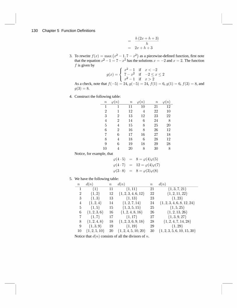
3. To rewrite i+{, @ pd{�{5 � 4> :� {5

�as a piecewise-de¿ned function,¿rst note

that the equation{5�4 @ :�{5 has the solutions{ @ �5 and{ @ 5. The functioni is given by

j+{, @

;?=

{5 � 4 if { ? �5:� {5 if �5 � { � 5{5 � 4 if { A 5

As a check, note thati+�8, @ 57, j+�8, @ 57, i+4, @ 9, j+4, @ 9, i+6, @ ;, andj+6, @ ;.

4. Construct the following table:q *+q, q *+q, q *+q,4 4 44 43 54 455 4 45 7 55 436 5 46 45 56 557 5 47 9 57 ;8 7 48 ; 58 539 5 49 ; 59 45: 9 4: 49 5: 4;; 7 4; 9 5; 45< 9 4< 4; 5< 5;43 7 53 ; 63 ;

Notice, for example, that*+7 � 8, @ ; @ *+7,*+8,

*+7 � :, @ 45 @ *+7,*+:,

*+6 � ;, @ ; @ *+6,*+;,

5. We have the following table:q g+q, q g+q, q g+q,4 i4j 44 i4> 44j 54 i4> 6> :> 54j5 i4> 5j 45 i4> 5> 6> 7> 9> 45j 55 i4> 5> 44> 55j6 i4> 6j 46 i4> 46j 56 i4> 56j7 i4> 5> 7j 47 i4> 5> :> 47j 57 i4> 5> 6> 7> 9> ;> 45> 57j8 i4> 8j 48 i4> 6> 8> 48j 58 i4> 8> 58j9 i4> 5> 6> 9j 49 i4> 5> 7> ;> 49j 59 i4> 5> 46> 59j: i4> :j 4: i4> 4:j 5: i4> 6> <> 5:j; i4> 5> 7> ;j 4; i4> 5> 6> 9> <> 4;j 5; i4> 5> 7> :> 47> 5;j< i4> 6> <j 4< i4> 4<j 5< i4> 5<j43 i4> 5> 8> 43j 53 i4> 5> 7> 8> 43> 53j 63 i4> 5> 6> 8> 9> 43> 48> 63j

Notice thatg+q, consists of all the divisors ofq.

Documents

4 Trigonometry and Complex · PDF file4 Trigonometry and Complex Numbers ... When any operation is applied to an angle represented in degrees by a mathematics superscript, such as