3`o - Julian Oliver · PDF fileBo Thid é Uppsala, Sweden All ... The cover graphics illustrates the linear momentum radiation pattern of a radio beam endowed with orbital angular

Draft version released 29th October 2012 at 16:48 CET—Downloaded from http://www.plasma.uu.se/CED/BookSheet: 1 of 294.

DRAFTBoFidé

electromagnetic

field theory

second edition


DRAFT


DRAFTELECTROMAGNETIC FIELD THEORY

Second Edition


DRAFT


DRAFTELECTROMAGNETIC

FIELD THEORY

Second Edition

Bo Thidé

Swedish Institute of Space Physics

Uppsala, Sweden

and

Department of Physics and Astronomy

Uppsala University, Sweden

and

Galilean School ofHigher Education

University of Padua

Padua, Italy


DRAFTAlso available

ELECTROMAGNETIC FIELD THEORY

EXERCISES

by

Tobia Carozzi, Anders Eriksson, Bengt Lundborg,Bo Thidé and Mattias Waldenvik

Freely downloadable fromwww.plasma.uu.se/CEDThis book was typeset in LATEX 2" based on TEX 3.1415926 and Web2C 7.5.6

Copyright ©1997–2011 byBo ThidéUppsala, SwedenAll rights reserved.

Electromagnetic Field TheoryISBN 978-0-486-4773-2

The cover graphics illustrates the linear momentum radiation pattern of a radio beam endowed with orbitalangular momentum, generated by an array of tri-axial antennas. This graphics illustration was prepared byJOHAN S JÖHOLM and KRISTOFFER PALMER as part of their undergraduate Diploma Thesis work in En-gineering Physics at Uppsala University 2006–2007.


DRAFTTo the memory of professor

LEV M IKHAILOVICH ERUKHIMOV (1936–1997)dear friend, great physicist, poet

and a truly remarkable man.


DRAFT


DRAFT

CONTENTS

Contents ix

List of Figures xv

Preface to the second edition xvii

Preface to the first edition xix

1 Foundations of Classical Electrodynamics 11.1 Electrostatics . . . . . . . . . . . . . . . . . . . . . . . . . . . . . . . . . . . . 2

1.1.1 Coulomb’s law . . . . . . . . . . . . . . . . . . . . . . . . . . . . . . . 21.1.2 The electrostatic field . . . . . . . . . . . . . . . . . . . . . . . . . . . . 3

1.2 Magnetostatics . . . . . . . . . . . . . . . . . . . . . . . . . . . . . . . . . . . 61.2.1 Ampère’s law . . . . . . . . . . . . . . . . . . . . . . . . . . . . . . . . 61.2.2 The magnetostatic field . . . . . . . . . . . . . . . . . . . . . . . . . . . 7

1.3 Electrodynamics . . . . . . . . . . . . . . . . . . . . . . . . . . . . . . . . . . . 91.3.1 The indestructibility of electric charge . . . . . . . . . . . . . . . . . . . 101.3.2 Maxwell’s displacement current . . . . . . . . . . . . . . . . . . . . . . 101.3.3 Electromotive force . . . . . . . . . . . . . . . . . . . . . . . . . . . . . 111.3.4 Faraday’s law of induction . . . . . . . . . . . . . . . . . . . . . . . . . 121.3.5 The microscopic Maxwell equations . . . . . . . . . . . . . . . . . . . . 151.3.6 Dirac’s symmetrised Maxwell equations . . . . . . . . . . . . . . . . . . 15

1.4 Examples . . . . . . . . . . . . . . . . . . . . . . . . . . . . . . . . . . . . . . 161.5 Bibliography . . . . . . . . . . . . . . . . . . . . . . . . . . . . . . . . . . . . . 18

2 Electromagnetic Fields and Waves 192.1 Axiomatic classical electrodynamics . . . . . . . . . . . . . . . . . . . . . . . . 192.2 Complex notation and physical observables . . . . . . . . . . . . . . . . . . . . 20

2.2.1 Physical observables and averages . . . . . . . . . . . . . . . . . . . . . 212.2.2 Maxwell equations in Majorana representation . . . . . . . . . . . . . . . 22

2.3 The wave equations for E and B . . . . . . . . . . . . . . . . . . . . . . . . . . 232.3.1 The time-independent wave equations for E and B . . . . . . . . . . . . 25


3 Electromagnetic Potentials and Gauges 333.1 The electrostatic scalar potential . . . . . . . . . . . . . . . . . . . . . . . . . . 333.2 The magnetostatic vector potential . . . . . . . . . . . . . . . . . . . . . . . . . 343.3 The electrodynamic potentials . . . . . . . . . . . . . . . . . . . . . . . . . . . 35

ix


DRAFT

x CONTENTS

3.4 Gauge conditions . . . . . . . . . . . . . . . . . . . . . . . . . . . . . . . . . . 363.4.1 Lorenz-Lorentz gauge . . . . . . . . . . . . . . . . . . . . . . . . . . . . 373.4.2 Coulomb gauge . . . . . . . . . . . . . . . . . . . . . . . . . . . . . . . 403.4.3 Velocity gauge . . . . . . . . . . . . . . . . . . . . . . . . . . . . . . . 42

3.5 Gauge transformations . . . . . . . . . . . . . . . . . . . . . . . . . . . . . . . 423.5.1 Other gauges . . . . . . . . . . . . . . . . . . . . . . . . . . . . . . . . 44


4 Fundamental Properties of the Electromagnetic Field 534.1 Discrete symmetries . . . . . . . . . . . . . . . . . . . . . . . . . . . . . . . . . 53

4.1.1 Charge conjugation, spatial inversion, and time reversal . . . . . . . . . . 534.1.2 C symmetry . . . . . . . . . . . . . . . . . . . . . . . . . . . . . . . . . 544.1.3 P symmetry . . . . . . . . . . . . . . . . . . . . . . . . . . . . . . . . . 554.1.4 T symmetry . . . . . . . . . . . . . . . . . . . . . . . . . . . . . . . . . 55

4.2 Continuous symmetries . . . . . . . . . . . . . . . . . . . . . . . . . . . . . . . 564.2.1 General conservation laws . . . . . . . . . . . . . . . . . . . . . . . . . 564.2.2 Conservation of electric charge . . . . . . . . . . . . . . . . . . . . . . . 584.2.3 Conservation of energy . . . . . . . . . . . . . . . . . . . . . . . . . . . 594.2.4 Conservation of linear (translational) momentum . . . . . . . . . . . . . 61

4.2.4.1 Gauge-invariant operator formalism . . . . . . . . . . . . . . . 634.2.5 Conservation of angular (rotational) momentum . . . . . . . . . . . . . . 66

4.2.5.1 Gauge-invariant operator formalism . . . . . . . . . . . . . . . 694.2.6 Electromagnetic duality . . . . . . . . . . . . . . . . . . . . . . . . . . . 714.2.7 Electromagnetic virial theorem . . . . . . . . . . . . . . . . . . . . . . . 72


5 Fields from Arbitrary Charge and Current Distributions 855.1 Fourier component method . . . . . . . . . . . . . . . . . . . . . . . . . . . . . 865.2 The retarded electric field . . . . . . . . . . . . . . . . . . . . . . . . . . . . . . 885.3 The retarded magnetic field . . . . . . . . . . . . . . . . . . . . . . . . . . . . . 915.4 The total electric and magnetic fields at large distances from the sources . . . . . 93

5.4.1 The far fields . . . . . . . . . . . . . . . . . . . . . . . . . . . . . . . . 985.5 Examples . . . . . . . . . . . . . . . . . . . . . . . . . . . . . . . . . . . . . . 100

6 Radiation and Radiating Systems 1016.1 Radiation of linear momentum and energy . . . . . . . . . . . . . . . . . . . . . 102

6.1.1 Monochromatic signals . . . . . . . . . . . . . . . . . . . . . . . . . . . 1036.1.2 Finite bandwidth signals . . . . . . . . . . . . . . . . . . . . . . . . . . 104

6.2 Radiation of angular momentum . . . . . . . . . . . . . . . . . . . . . . . . . . 105


DRAFT

CONTENTS xi

6.3 Radiation from a localised source at rest . . . . . . . . . . . . . . . . . . . . . . 1066.3.1 Electric multipole moments . . . . . . . . . . . . . . . . . . . . . . . . . 1066.3.2 The Hertz potential . . . . . . . . . . . . . . . . . . . . . . . . . . . . . 1076.3.3 Electric dipole radiation . . . . . . . . . . . . . . . . . . . . . . . . . . . 1116.3.4 Magnetic dipole radiation . . . . . . . . . . . . . . . . . . . . . . . . . . 1136.3.5 Electric quadrupole radiation . . . . . . . . . . . . . . . . . . . . . . . . 114

6.4 Radiation from an extended source volume at rest . . . . . . . . . . . . . . . . . 1156.4.1 Radiation from a one-dimensional current distribution . . . . . . . . . . . 115

6.5 Radiation from a localised charge in arbitrary motion . . . . . . . . . . . . . . . 1196.5.1 The Liénard-Wiechert potentials . . . . . . . . . . . . . . . . . . . . . . 1216.5.2 Radiation from an accelerated point charge . . . . . . . . . . . . . . . . 123

6.5.2.1 The differential operator method . . . . . . . . . . . . . . . . . 1246.5.2.2 The direct method . . . . . . . . . . . . . . . . . . . . . . . . 1276.5.2.3 Small velocities . . . . . . . . . . . . . . . . . . . . . . . . . . 129

6.5.3 Bremsstrahlung . . . . . . . . . . . . . . . . . . . . . . . . . . . . . . . 1306.5.4 Cyclotron and synchrotron radiation . . . . . . . . . . . . . . . . . . . . 133

6.5.4.1 Cyclotron radiation . . . . . . . . . . . . . . . . . . . . . . . . 1356.5.4.2 Synchrotron radiation . . . . . . . . . . . . . . . . . . . . . . 1366.5.4.3 Radiation in the general case . . . . . . . . . . . . . . . . . . . 1386.5.4.4 Virtual photons . . . . . . . . . . . . . . . . . . . . . . . . . . 139


7 Relativistic Electrodynamics 1517.1 The special theory of relativity . . . . . . . . . . . . . . . . . . . . . . . . . . . 151

7.1.1 The Lorentz transformation . . . . . . . . . . . . . . . . . . . . . . . . . 1527.1.2 Lorentz space . . . . . . . . . . . . . . . . . . . . . . . . . . . . . . . . 153

7.1.2.1 Radius four-vector in contravariant and covariant form . . . . . 1547.1.2.2 Scalar product and norm . . . . . . . . . . . . . . . . . . . . . 1547.1.2.3 Metric tensor . . . . . . . . . . . . . . . . . . . . . . . . . . . 1547.1.2.4 Invariant line element and proper time . . . . . . . . . . . . . . 1567.1.2.5 Four-vector fields . . . . . . . . . . . . . . . . . . . . . . . . . 1577.1.2.6 The Lorentz transformation matrix . . . . . . . . . . . . . . . . 1587.1.2.7 The Lorentz group . . . . . . . . . . . . . . . . . . . . . . . . 158

7.1.3 Minkowski space . . . . . . . . . . . . . . . . . . . . . . . . . . . . . . 1587.2 Covariant classical mechanics . . . . . . . . . . . . . . . . . . . . . . . . . . . . 1607.3 Covariant classical electrodynamics . . . . . . . . . . . . . . . . . . . . . . . . 162

7.3.1 The four-potential . . . . . . . . . . . . . . . . . . . . . . . . . . . . . . 1627.3.2 The Liénard-Wiechert potentials . . . . . . . . . . . . . . . . . . . . . . 1637.3.3 The electromagnetic field tensor . . . . . . . . . . . . . . . . . . . . . . 165

7.4 Bibliography . . . . . . . . . . . . . . . . . . . . . . . . . . . . . . . . . . . . . 169


DRAFT

xii CONTENTS

8 Electromagnetic Fields and Particles 1718.1 Charged particles in an electromagnetic field . . . . . . . . . . . . . . . . . . . . 171

8.1.1 Covariant equations of motion . . . . . . . . . . . . . . . . . . . . . . . 1718.1.1.1 Lagrangian formalism . . . . . . . . . . . . . . . . . . . . . . 1718.1.1.2 Hamiltonian formalism . . . . . . . . . . . . . . . . . . . . . . 174

8.2 Covariant field theory . . . . . . . . . . . . . . . . . . . . . . . . . . . . . . . . 1778.2.1 Lagrange-Hamilton formalism for fields and interactions . . . . . . . . . 178

8.2.1.1 The electromagnetic field . . . . . . . . . . . . . . . . . . . . 1818.2.1.2 Other fields . . . . . . . . . . . . . . . . . . . . . . . . . . . . 184

8.3 Bibliography . . . . . . . . . . . . . . . . . . . . . . . . . . . . . . . . . . . . . 185

9 Electromagnetic Fields and Matter 1879.1 Maxwell’s macroscopic theory . . . . . . . . . . . . . . . . . . . . . . . . . . . 188

9.1.1 Polarisation and electric displacement . . . . . . . . . . . . . . . . . . . 1889.1.2 Magnetisation and the magnetising field . . . . . . . . . . . . . . . . . . 1899.1.3 Macroscopic Maxwell equations . . . . . . . . . . . . . . . . . . . . . . 191

9.2 Phase velocity, group velocity and dispersion . . . . . . . . . . . . . . . . . . . 1929.3 Radiation from charges in a material medium . . . . . . . . . . . . . . . . . . . 193

9.3.1 Vavilov- LCerenkov radiation . . . . . . . . . . . . . . . . . . . . . . . . . 1939.4 Electromagnetic waves in a medium . . . . . . . . . . . . . . . . . . . . . . . . 198

9.4.1 Constitutive relations . . . . . . . . . . . . . . . . . . . . . . . . . . . . 1999.4.2 Electromagnetic waves in a conducting medium . . . . . . . . . . . . . . 201

9.4.2.1 The wave equations for E and B . . . . . . . . . . . . . . . . . 2019.4.2.2 Plane waves . . . . . . . . . . . . . . . . . . . . . . . . . . . 2029.4.2.3 Telegrapher’s equation . . . . . . . . . . . . . . . . . . . . . . 203

9.5 Bibliography . . . . . . . . . . . . . . . . . . . . . . . . . . . . . . . . . . . . . 209

F Formulæ 211F.1 Vector and tensor fields in 3D Euclidean space . . . . . . . . . . . . . . . . . . . 211

F.1.1 Cylindrical circular coordinates . . . . . . . . . . . . . . . . . . . . . . . 212F.1.1.1 Base vectors . . . . . . . . . . . . . . . . . . . . . . . . . . . 212F.1.1.2 Directed line element . . . . . . . . . . . . . . . . . . . . . . . 212F.1.1.3 Directed area element . . . . . . . . . . . . . . . . . . . . . . 212F.1.1.4 Volume element . . . . . . . . . . . . . . . . . . . . . . . . . 212F.1.1.5 Spatial differential operators . . . . . . . . . . . . . . . . . . . 212

F.1.2 Spherical polar coordinates . . . . . . . . . . . . . . . . . . . . . . . . . 213F.1.2.1 Base vectors . . . . . . . . . . . . . . . . . . . . . . . . . . . 213F.1.2.2 Directed line element . . . . . . . . . . . . . . . . . . . . . . . 213F.1.2.3 Solid angle element . . . . . . . . . . . . . . . . . . . . . . . 213F.1.2.4 Directed area element . . . . . . . . . . . . . . . . . . . . . . 213F.1.2.5 Volume element . . . . . . . . . . . . . . . . . . . . . . . . . 214


DRAFT

CONTENTS xiii

F.1.2.6 Spatial differential operators . . . . . . . . . . . . . . . . . . . 214F.1.3 Vector and tensor field formulæ . . . . . . . . . . . . . . . . . . . . . . . 214

F.1.3.1 The three-dimensional unit tensor of rank two . . . . . . . . . . 214F.1.3.2 The 3D Kronecker delta tensor . . . . . . . . . . . . . . . . . . 215F.1.3.3 The fully antisymmetric Levi-Civita tensor . . . . . . . . . . . 215F.1.3.4 Rotational matrices . . . . . . . . . . . . . . . . . . . . . . . . 215F.1.3.5 General vector and tensor algebra identities . . . . . . . . . . . 216F.1.3.6 Special vector and tensor algebra identities . . . . . . . . . . . 216F.1.3.7 General vector and tensor calculus identities . . . . . . . . . . 217F.1.3.8 Special vector and tensor calculus identities . . . . . . . . . . . 218F.1.3.9 Integral identities . . . . . . . . . . . . . . . . . . . . . . . . . 219

F.2 The electromagnetic field . . . . . . . . . . . . . . . . . . . . . . . . . . . . . . 221F.2.1 Microscopic Maxwell-Lorentz equations in Dirac’s symmetrised form . . 221

F.2.1.1 Constitutive relations . . . . . . . . . . . . . . . . . . . . . . . 221F.2.2 Fields and potentials . . . . . . . . . . . . . . . . . . . . . . . . . . . . 222

F.2.2.1 Vector and scalar potentials . . . . . . . . . . . . . . . . . . . 222F.2.2.2 The velocity gauge condition in free space . . . . . . . . . . . 222F.2.2.3 Gauge transformation . . . . . . . . . . . . . . . . . . . . . . 222

F.2.3 Energy and momentum . . . . . . . . . . . . . . . . . . . . . . . . . . . 222F.2.3.1 Electromagnetic field energy density in free space . . . . . . . 222F.2.3.2 Poynting vector in free space . . . . . . . . . . . . . . . . . . . 222F.2.3.3 Linear momentum density in free space . . . . . . . . . . . . . 222F.2.3.4 Linear momentum flux tensor in free space . . . . . . . . . . . 223F.2.3.5 Angular momentum density around x0 in free space . . . . . . 223F.2.3.6 Angular momentum flux tensor around x0 in free space . . . . 223

F.2.4 Electromagnetic radiation . . . . . . . . . . . . . . . . . . . . . . . . . . 223F.2.4.1 The far fields from an extended source distribution . . . . . . . 223F.2.4.2 The far fields from an electric dipole . . . . . . . . . . . . . . . 223F.2.4.3 The far fields from a magnetic dipole . . . . . . . . . . . . . . 224F.2.4.4 The far fields from an electric quadrupole . . . . . . . . . . . . 224F.2.4.5 Relationship between the field vectors in a plane wave . . . . . 224F.2.4.6 The fields from a point charge in arbitrary motion . . . . . . . . 224

F.3 Special relativity . . . . . . . . . . . . . . . . . . . . . . . . . . . . . . . . . . . 225F.3.1 Metric tensor for flat 4D space . . . . . . . . . . . . . . . . . . . . . . . 225F.3.2 Lorentz transformation of a four-vector . . . . . . . . . . . . . . . . . . 225F.3.3 Covariant and contravariant four-vectors . . . . . . . . . . . . . . . . . . 225

F.3.3.1 Position four-vector (radius four-vector) . . . . . . . . . . . . . 225F.3.3.2 Arbitrary four-vector field . . . . . . . . . . . . . . . . . . . . 225F.3.3.3 Four-del operator . . . . . . . . . . . . . . . . . . . . . . . . . 226F.3.3.4 Invariant line element . . . . . . . . . . . . . . . . . . . . . . 226F.3.3.5 Four-velocity . . . . . . . . . . . . . . . . . . . . . . . . . . . 226


DRAFT

xiv CONTENTS

F.3.3.6 Four-momentum . . . . . . . . . . . . . . . . . . . . . . . . . 226F.3.3.7 Four-current density . . . . . . . . . . . . . . . . . . . . . . . 226F.3.3.8 Four-potential . . . . . . . . . . . . . . . . . . . . . . . . . . 226

F.3.4 Field tensor . . . . . . . . . . . . . . . . . . . . . . . . . . . . . . . . . 226F.4 Bibliography . . . . . . . . . . . . . . . . . . . . . . . . . . . . . . . . . . . . . 227

M Mathematical Methods 229M.1 Scalars, vectors and tensors . . . . . . . . . . . . . . . . . . . . . . . . . . . . . 230

M.1.1 Vectors . . . . . . . . . . . . . . . . . . . . . . . . . . . . . . . . . . . 231M.1.1.1 Position vector . . . . . . . . . . . . . . . . . . . . . . . . . . 231

M.1.2 Fields . . . . . . . . . . . . . . . . . . . . . . . . . . . . . . . . . . . . 232M.1.2.1 Scalar fields . . . . . . . . . . . . . . . . . . . . . . . . . . . . 232M.1.2.2 Vector fields . . . . . . . . . . . . . . . . . . . . . . . . . . . 233M.1.2.3 Coordinate transformations . . . . . . . . . . . . . . . . . . . 233M.1.2.4 Tensor fields . . . . . . . . . . . . . . . . . . . . . . . . . . . 234

M.2 Vector algebra . . . . . . . . . . . . . . . . . . . . . . . . . . . . . . . . . . . . 237M.2.1 Scalar product . . . . . . . . . . . . . . . . . . . . . . . . . . . . . . . . 237M.2.2 Vector product . . . . . . . . . . . . . . . . . . . . . . . . . . . . . . . . 237M.2.3 Dyadic product . . . . . . . . . . . . . . . . . . . . . . . . . . . . . . . 238

M.3 Vector calculus . . . . . . . . . . . . . . . . . . . . . . . . . . . . . . . . . . . 240M.3.1 The del operator . . . . . . . . . . . . . . . . . . . . . . . . . . . . . . . 240M.3.2 The gradient of a scalar field . . . . . . . . . . . . . . . . . . . . . . . . 241M.3.3 The divergence of a vector field . . . . . . . . . . . . . . . . . . . . . . 241M.3.4 The curl of a vector field . . . . . . . . . . . . . . . . . . . . . . . . . . 241M.3.5 The Laplacian . . . . . . . . . . . . . . . . . . . . . . . . . . . . . . . . 242M.3.6 Vector and tensor integrals . . . . . . . . . . . . . . . . . . . . . . . . . 242

M.3.6.1 First order derivatives . . . . . . . . . . . . . . . . . . . . . . 243M.3.6.2 Second order derivatives . . . . . . . . . . . . . . . . . . . . . 244

M.3.7 Helmholtz’s theorem . . . . . . . . . . . . . . . . . . . . . . . . . . . . 245M.4 Analytical mechanics . . . . . . . . . . . . . . . . . . . . . . . . . . . . . . . . 247

M.4.1 Lagrange’s equations . . . . . . . . . . . . . . . . . . . . . . . . . . . . 247M.4.2 Hamilton’s equations . . . . . . . . . . . . . . . . . . . . . . . . . . . . 248

M.5 Examples . . . . . . . . . . . . . . . . . . . . . . . . . . . . . . . . . . . . . . 248M.6 Bibliography . . . . . . . . . . . . . . . . . . . . . . . . . . . . . . . . . . . . . 263

Index 265


DRAFT

LIST OF FIGURES

1.1 Coulomb interaction between two electric charges . . . . . . . . . . . . . . . . . . . 31.2 Coulomb interaction for a distribution of electric charges . . . . . . . . . . . . . . . 51.3 Ampère interaction . . . . . . . . . . . . . . . . . . . . . . . . . . . . . . . . . . . 71.4 Moving loop in a varying B field . . . . . . . . . . . . . . . . . . . . . . . . . . . . 13

5.1 Fields in the far zone . . . . . . . . . . . . . . . . . . . . . . . . . . . . . . . . . . 94

6.1 Multipole radiation geometry . . . . . . . . . . . . . . . . . . . . . . . . . . . . . . 1096.2 Electric dipole geometry . . . . . . . . . . . . . . . . . . . . . . . . . . . . . . . . 1126.3 Linear antenna . . . . . . . . . . . . . . . . . . . . . . . . . . . . . . . . . . . . . . 1176.4 Electric dipole antenna geometry . . . . . . . . . . . . . . . . . . . . . . . . . . . . 1186.5 Radiation from a moving charge in vacuum . . . . . . . . . . . . . . . . . . . . . . 1206.6 An accelerated charge in vacuum . . . . . . . . . . . . . . . . . . . . . . . . . . . . 1226.7 Angular distribution of radiation during bremsstrahlung . . . . . . . . . . . . . . . . 1306.8 Location of radiation during bremsstrahlung . . . . . . . . . . . . . . . . . . . . . . 1326.9 Radiation from a charge in circular motion . . . . . . . . . . . . . . . . . . . . . . . 1346.10 Synchrotron radiation lobe width . . . . . . . . . . . . . . . . . . . . . . . . . . . . 1376.11 The perpendicular electric field of a moving charge . . . . . . . . . . . . . . . . . . 1396.12 Electron-electron scattering . . . . . . . . . . . . . . . . . . . . . . . . . . . . . . . 1406.13 Loop antenna . . . . . . . . . . . . . . . . . . . . . . . . . . . . . . . . . . . . . . 143

7.1 Relative motion of two inertial systems . . . . . . . . . . . . . . . . . . . . . . . . . 1527.2 Rotation in a 2D Euclidean space . . . . . . . . . . . . . . . . . . . . . . . . . . . . 1597.3 Minkowski diagram . . . . . . . . . . . . . . . . . . . . . . . . . . . . . . . . . . . 160

8.1 Linear one-dimensional mass chain . . . . . . . . . . . . . . . . . . . . . . . . . . . 178

9.1 Vavilov- LCerenkov cone . . . . . . . . . . . . . . . . . . . . . . . . . . . . . . . . . 195

M.1 Tetrahedron-like volume element of matter . . . . . . . . . . . . . . . . . . . . . . . 250

xv


DRAFT


DRAFT

PREFACE TO THE SECOND EDITION

This second edition of the book ELECTROMAGNETIC F IELD THEORY is a major revisionand expansion of the first edition that was published on the Internet (www.plasma.uu.se/CED/Book) in an organic growth process over the years 1997–2008. The main changes are an expan-sion of the material treated, an addition of a new chapter and several illustrative examples, and aslight reordering of the chapters.

The main reason for attempting to improve the presentation and to add more material is thatthis new edition is now being made available in printed form by Dover Publications and is used inan extended Classical Electrodynamics course at Uppsala University, at the last-year undergradu-ate, Master, and beginning post-graduate/doctoral level. It has also been used by the author in asimilar course at the Galilean School of Higher Education (Scuola Galileiana di Studi Superiori)at University of Padova. It is the author’s hope that the second edition of his book will find a widuse in Academia and elsewhere.

The subject matter starts with a description of the properties of electromagnetism when thecharges and currents are located in otherwise free space, i.e., a space that is free of matter andexternal fields (e.g., gravitation). A rigorous analysis of the fundamental properties of the elec-tromagnetic fields and radiation phenomena follows. Only then the influence of matter on thefields and the pertinent interaction processes is taken into account. In the author’s opinion, thisapproach is preferable since it avoids the formal logical inconsistency of introducing, very earlyin the derivations, the effect on the electric and mangetic fields when conductors and dielectricsare present (and vice versa) in an ad hoc manner, before constitutive relations and physical mod-els for the electromagnetic properties of matter, including conductors and dielectrics, have beenderived from first principles. Curved-space effects on electromagnetism are not treated at all.

In addition to the Maxwell-Lorentz equations, which postulate the beaviour of electromag-netic fields due to electric charges and currents on a microscopic classical scale, chapter chapter 1also introduces Dirac’s symmetrised equations that incorporate the effects of magnetic chargesand currents. In chapter chapter 2, a stronger emphasis than before is put on the axiomatic found-ation of electrodynamics as provided by the Maxwell-Lorentz equations that are taken as thepostulates of the theory. Chapter chapter 3 on potentials and gauges now provides a more com-prehensive picture and discusses gauge invariance in a more satisfactory manner than the firstedition did. Chapter chapter 4 is new and deals with symmetries and conserved quantities in amore rigourous, profound and detailed way than in the first edition. For instance, the presentationof the theory of electromagnetic angular momentum and other observables (constants of motion)has been substantially expanded and put on a firm basis. Chapter chapter 9 is a complete rewriteand combines material that was scattered more or less all over the first edition. It also containsnew material on wave propagation in plasma and other media. When, in chapter chapter 9, themacroscopic Maxwell equations are introduced, the inherent approximations in the derived fieldquantities are clearly pointed out. The collection of formulæ in appendix F on page 211 has beenaugmented quite substantially. In appendix M on page 229, the treatment of dyadic products andtensors has been expanded significantly and numerous examples have been added throughout.

xvii

www.plasma.uu.se/CED/Book

www.plasma.uu.se/CED/Book


DRAFT

xviii PREFACE TO THE SECOND EDITION

I want to express my warm gratitude to professor CESARE BARBIERI and his entire group,particularly FABRIZIO TAMBURINI, at the Department of Astronomy, University of Padova,for stimulating discussions and the generous hospitality bestowed upon me during several shorterand longer visits in 2008, 2009, and 2010 that made it possible to prepare the current major revi-sion of the book. In this breathtakingly beautiful northern Italy where the cradle of renaissanceonce stood, intellectual titan GALILEO GALILEI worked for eighteen years and gave birth tomodern physics, astronomy and science as we know it today, by sweeping away Aristotelian dog-mas, misconceptions and mere superstition, thus most profoundly changing our conception of theworld and our place in it. In the process, Galileo’s new ideas transformed society and mankindirreversibly and changed our view of the Universe, including our own planet, forever. It is hopedthat this book may contribute in some small, humble way to further these, once upon a time,mind-boggling—and dangerous—ideas of intellectual freedom and enlightment.

Thanks are also due to JOHAN S JÖHOLM, KRISTOFFER PALMER, MARCUS ERIKS-SON, and JOHAN L INDBERG who during their work on their Diploma theses suggested im-provements and additions and to HOLGER THEN and STAFFAN YNGVE for carefully checkingsome lengthy calculations and to the numerous undergraduate students, who have been exposedto various draft versions of this second edtion. In particular, I would like to mention BRUNO

STRANDBERG.This book is dedicated to my son MATTIAS, my daughter KAROLINA, my four grandsons

MAX , ALBIN , F IL IP and OSKAR, my high-school physics teacher, STAFFAN RÖSBY, andmy fellow members of the CAPELLA PEDAGOGICA UPSALIENSIS.

Padova, Italy BO THIDÉ

February, 2011 www.physics.irfu.se/�bt


DRAFT

PREFACE TO THE FIRST EDITION

Of the four known fundamental interactions in nature—gravitational, strong, weak, and electro-magnetic—the latter has a special standing in the physical sciences. Not only does it, togetherwith gravitation, permanently make itself known to all of us in our everyday lives. Electro-dynamics is also by far the most accurate physical theory known, tested on scales running fromsub-nuclear to galactic, and electromagnetic field theory is the prototype of all other field theories.

This book, ELECTROMAGNETIC F IELD THEORY, which tries to give a modern view ofclassical electrodynamics, is the result of a more than thirty-five year long love affair. In theautumn of 1972, I took my first advanced course in electrodynamics at the Department of Theor-etical Physics, Uppsala University. Soon I joined the research group there and took on the taskof helping the late professor PER OLOF FRÖMAN, who was to become my Ph.D. thesis ad-viser, with the preparation of a new version of his lecture notes on the Theory of Electricity. Thisopened my eyes to the beauty and intricacy of electrodynamics and I simply became intrigued byit. The teaching of a course in Classical Electrodynamics at Uppsala University, some twenty oddyears after I experienced the first encounter with the subject, provided the incentive and impetusto write this book.

Intended primarily as a textbook for physics and engineering students at the advanced under-graduate or beginning graduate level, it is hoped that the present book will be useful for researchworkers too. It aims at providing a thorough treatment of the theory of electrodynamics, mainlyfrom a classical field-theoretical point of view. The first chapter is, by and large, a descrip-tion of how Classical Electrodynamics was established by JAMES CLERK MAXWELL as afundamental theory of nature. It does so by introducing electrostatics and magnetostatics anddemonstrating how they can be unified into one theory, classical electrodynamics, summarisedin Lorentz’s microscopic formulation of the Maxwell equations. These equations are used as anaxiomatic foundation for the treatment in the remainder of the book, which includes modern for-mulation of the theory; electromagnetic waves and their propagation; electromagnetic potentialsand gauge transformations; analysis of symmetries and conservation laws describing the elec-tromagnetic counterparts of the classical concepts of force, momentum and energy, plus otherfundamental properties of the electromagnetic field; radiation phenomena; and covariant Lag-rangian/Hamiltonian field-theoretical methods for electromagnetic fields, particles and interac-tions. Emphasis has been put on modern electrodynamics concepts while the mathematical toolsused, some of them presented in an Appendix, are essentially the same kind of vector and tensoranalysis methods that are used in intermediate level textbooks on electromagnetics but perhaps abit more advanced and far-reaching.

The aim has been to write a book that can serve both as an advanced text in Classical Elec-trodynamics and as a preparation for studies in Quantum Electrodynamics and Field Theory, aswell as more applied subjects such as Plasma Physics, Astrophysics, Condensed Matter Physics,Optics, Antenna Engineering, and Wireless Communications.

The current version of the book is a major revision of an earlier version, which in turn was anoutgrowth of the lecture notes that the author prepared for the four-credit course Electrodynam-

xix


DRAFT

xx PREFACE TO THE FIRST EDITION

ics that was introduced in the Uppsala University curriculum in 1992, to become the five-creditcourse Classical Electrodynamics in 1997. To some extent, parts of those notes were based onlecture notes prepared, in Swedish, by my friend and Theoretical Physics colleague BENGT

LUNDBORG, who created, developed and taught an earlier, two-credit course called Electro-magnetic Radiation at our faculty. Thanks are due not only to Bengt Lundborg for providingthe inspiration to write this book, but also to professor CHRISTER WAHLBERG, and professorGÖRAN FÄLDT, both at the Department of Physics and Astronomy, Uppsala University, forinsightful suggestions, to professor JOHN LEARNED, Department of Physics and Astronomy,University of Hawaii, for decisive encouragement at the early stage of this book project, to pro-fessor GERARDUS T’HOOFT, for recommending this book on his web page ‘How to becomea good theoretical physicist’, and professor CECILIA JARLSKOG, Lund Unversity, for pointingout a couple of errors and ambiguities.

I am particularly indebted to the late professor V ITALIY LAZAREVICH G INZBURG, forhis many fascinating and very elucidating lectures, comments and historical notes on plasmaphysics, electromagnetic radiation and cosmic electrodynamics while cruising up and down theVolga and Oka rivers in Russia at the ship-borne Russian-Swedish summer schools that wereorganised jointly by late professor LEV M IKAHILOVICH ERUKHIMOV and the author duringthe 1990’s, and for numerous deep discussions over the years.

Helpful comments and suggestions for improvement from former PhD students TOBIA CA-ROZZI, ROGER KARLSSON, and MATTIAS WALDENVIK, as well as ANDERS ERIKSSON

at the Swedish Institute of Space Physics in Uppsala and who have all taught Uppsala studentson the material covered in this book, are gratefully acknowledged. Thanks are also due to the lateHELMUT KOPKA, for more than twenty-five years a close friend and space physics colleagueworking at the Max-Planck-Institut für Aeronomie, Lindau, Germany, who not only taught methe practical aspects of the use of high-power electromagnetic radiation for studying space, butalso some of the delicate aspects of typesetting in TEX and LATEX.

In an attempt to encourage the involvement of other scientists and students in the making ofthis book, thereby trying to ensure its quality and scope to make it useful in higher universityeducation anywhere in the world, it was produced as a World-Wide Web (WWW) project. Thisturned out to be a rather successful move. By making an electronic version of the book freelydownloadable on the Internet, comments have been received from fellow physicists around theworld. To judge from WWW ‘hit’ statistics, it seems that the book serves as a frequently usedInternet resource. This way it is hoped that it will be particularly useful for students and research-ers working under financial or other circumstances that make it difficult to procure a printed copyof the book. I would like to thank all students and Internet users who have downloaded andcommented on the book during its life on the World-Wide Web.

Uppsala, Sweden BO THIDÉ

December, 2008 www.physics.irfu.se/�bt


DRAFT1

FOUNDATIONS OF CLASSICAL

ELECTRODYNAMICS

The classical theory of electromagnetism deals with electric and magnetic fieldsand their interaction with each other and with charges and currents. This theoryis classical in the sense that it assumes the validity of certain mathematical limit-ing processes in which it is considered possible for the charge and current distri-butions to be localised in infinitesimally small volumes of space.1 Clearly, this 1 Accepting the mere existence of

an electrically charged particle re-quires some careful thinking. In hisexcellent book Classical ChargedParticles, FRITZ ROHRLICHwrites

‘To what extent does itmake sense to talk about anelectron, say, in classicalterms? These and similarquestions clearly indicatethat ignoring philosophyin physics means notunderstanding physics.For there is no theoreticalphysics without somephilosophy; not admittingthis fact would be self-deception.’

is in contradistinction to electromagnetism on an atomistic scale, where chargesand currents have to be described in a nonlocal quantum formalism. However,the limiting processes used in the classical domain, which, crudely speaking, as-sume that an elementary charge has a continuous distribution of charge density,will yield results that agree perfectly with experiments on non-atomistic scales,however small or large these scales may be.2

2 Electrodynamics has been testedexperimentally over a larger rangeof spatial scales than any otherexisting physical theory.

It took the genius of JAMES CLERK MAXWELL to consistently unify, inthe mid-1800’s, the theory of Electricity and the then distinctively different the-ory Magnetism into a single super-theory, Electromagnetism or Classical Elec-trodynamics (CED), and also to realise that optics is a sub-field of this super-theory. Early in the 20th century, HENDRIK ANTOON LORENTZ took theelectrodynamics theory further to the microscopic scale and also paved the wayfor the Special Theory of Relativity, formulated in its full extent by ALBERT

E INSTEIN in 1905. In the 1930’s PAUL ADRIEN MAURICE D IRAC expan-ded electrodynamics to a more symmetric form, including magnetic as well aselectric charges. With his relativistic quantum mechanics and field quantisationconcepts, Dirac had already in the 1920’s laid the foundation for Quantum Elec-trodynamics (QED ), the relativistic quantum theory for electromagnetic fieldsand their interaction with matter for which R ICHARD PHILLIPS FEYNMAN,JULIAN SEYMOUR SCHWINGER, and S IN- ITIRO TOMONAGA were awar-ded the Nobel Prize in Physics in 1965. Around the same time, physicists suchas SHELDON GLASHOW, ABDUS SALAM, and STEVEN WEINBERG wereable to unify electrodynamics with the weak interaction theory, thus creatingyet another successful super-theory, Electroweak Theory, an achievement whichrendered them the Nobel Prize in Physics 1979. The modern theory of stronginteractions, Quantum Chromodynamics (QCD ), is heavily influenced by CEDand QED.

1


DRAFT

2 j 1. FOUNDATIONS OF CLASSICAL ELECTRODYNAMICS

In this introductory chapter we start with the force interactions in classicalelectrostatics and classical magnetostatics, introduce the corresponding staticelectric and magnetic fields and postulate two uncoupled systems of differentialequations for them. We continue by showing that the conservation of electriccharge and its relation to electric current lead to a dynamic connection betweenelectricity and magnetism and how the two can be unified into Classical Elec-trodynamics. This theory is described by a system of coupled dynamic fieldequations — the microscopic versions of Maxwell’s differential equations intro-duced by Lorentz — which, in chapter 2, we take as the axiomatic foundation ofthe theory of electromagnetic fields and the basis for the treatment in the rest ofthe book.

At the end of this chapter 1 we present Dirac’s symmetrised form of theMaxwell-Lorentz equations that incorporate magnetic charges and magnetic cur-rents into the theory in a symmetric way. In practical work, such as in antennaengineering, magnetic currents have proved to be a very useful concept. Weshall make some use of this symmetrised theory of electricity and magnetism.

1.1 Electrostatics

The theory that describes physical phenomena related to the interaction betweenstationary electric charges or charge distributions in a finite space with station-ary boundaries is called electrostatics . For a long time, electrostatics, underthe name electricity, was considered an independent physical theory of its own,alongside other physical theories such as Magnetism, Mechanics, Optics, andThermodynamics.3

3 The physicist, mathematician andphilosopher P IERRE MAURICEMARIE DUHEM (1861–1916)once wrote:

‘The whole theory ofelectrostatics constitutesa group of abstract ideasand general propositions,formulated in the clearand concise language ofgeometry and algebra,and connected with oneanother by the rules ofstrict logic. This wholefully satisfies the reason ofa French physicist and histaste for clarity, simplicityand order. . . .’

1.1.1 Coulomb’s law

It has been found experimentally that the force interaction between stationary,electrically charged bodies can be described in terms of two-body mechanicalforces. Based on these experimental observations, Coulomb4 postulated, in

4 CHARLES-AUGUSTIN DECOULOMB (1736–1806) wasa French physicist who in 1775published three reports on theforces between electrically chargedbodies.

1775, that in the simple case depicted in figure 1.1 on the facing page, the mech-anical force on a static electric charge q located at the field point (observationpoint) x, due to the presence of another stationary electric charge q0 at the sourcepoint x0, is directed along the line connecting these two points, repulsive forcharges of equal signs and attractive for charges of opposite signs. This postu-


DRAFT

1.1. Electrostatics j 3

q0

q

O

x0

x � x0

x

Figure 1.1: Coulomb’s law pos-tulates that a static electric chargeq, located at a point x relative tothe origin O , will experience anelectrostatic force F es.x/ from astatic electric charge q0 located atx0. Note that this definition is inde-pendent of any particular choice ofcoordinate system since the mech-anical force F es is a true (polar)vector.

late is called Coulomb’s law and can be formulated mathematically as

F es.x/ Dqq0

4�"0

x � x0

jx � x0j3D �

qq0

4�"0r

�1

jx � x0j

�D

qq0

4�"0r 0�

1

jx � x0j

�(1.1)

where, in the last step, formula (F.114) on page 218 was used. In SI units , whichwe shall use throughout, the electrostatic force5 F es is measured in Newton (N), 5 Massive particles also interact

gravitationally but with a force thatis typically 10�36 times weaker.

the electric charges q and q0 in Coulomb (C), i.e. Ampere-seconds (As), andthe length jx � x0j in metres (m). The constant "0 D 107=.4�c2/ Farad permetre (Fm�1) is the permittivity of free space and c ms�1 is the speed of lightin vacuum.6 In CGS units , "0 D 1=.4�/ and the force is measured in dyne, 6 The notation c for speed stems

from the Latin word ‘celeritas’which means ‘swiftness’. Thisnotation seems to have been intro-duced by W ILHELM EDUARDWEBER (1804–1891), andRUDOLF KOHLRAUSCH (1809–1858) and c is therefore sometimesreferred to as Weber’s constant .In all his works from 1907 andonward, ALBERT E INSTEIN(1879–1955) used c to denote thespeed of light in free space.

electric charge in statcoulomb, and length in centimetres (cm).

1.1.2 The electrostatic field

Instead of describing the electrostatic interaction in terms of a ‘force action at adistance’, it turns out that for many purposes it is useful to introduce the conceptof a field. Thus we describe the electrostatic interaction in terms of a staticvectorial electric field Estat defined by the limiting process

Estat.x/def� lim

q!0

F es.x/

q(1.2)

where F es is the electrostatic force, as defined in equation (1.1) above, from a netelectric charge q0 on the test particle with a small net electric charge q. In the SIsystem of units, electric fields are therefore measured in NC�1 or, equivalently,in Vm�1. Since the purpose of the limiting process is to ascertain that the testcharge q does not distort the field set up by q0, the expression for Estat doesnot depend explicitly on q but only on the charge q0 and the relative positionvector x � x0. This means that we can say that any net electric charge produces


DRAFT


an electric field in the space that surrounds it, regardless of the existence of asecond charge anywhere in this space.7 However, in order to experimentally7 In the preface to the first edition

of the first volume of his bookA Treatise on Electricity andMagnetism, first published in 1873,Maxwell describes this in thefollowing almost poetic manner:

‘For instance, Faraday, inhis mind’s eye, saw lines offorce traversing all spacewhere the mathematicianssaw centres of forceattracting at a distance:Faraday saw a mediumwhere they saw nothingbut distance: Faradaysought the seat of thephenomena in real actionsgoing on in the medium,they were satisfied that theyhad found it in a powerof action at a distanceimpressed on the electricfluids.’

detect a charge, a second (test) charge that senses the presence of the first one,must be introduced.

Using equations (1.1) and (1.2) on the previous page, and formula (F.114)on page 218, we find that the electrostatic field Estat at the observation point x

(also known as the field point), due to a field-producing electric charge q0 at thesource point x0, is given by

Estat.x/ Dq0

4�"0

x � x0

jx � x0j3D �

q0

4�"0r

�1

jx � x0j

�D

q0

4�"0r 0�

1

jx � x0j

�(1.3)

In the presence of several field producing discrete electric charges q0i , locatedat the points x0i , i D 1; 2; 3; : : : , respectively, in otherwise empty space, theassumption of linearity of vacuum8 allows us to superimpose their individual

8 In fact, a vacuum exhibits aquantum mechanical non-linearitydue to vacuum polarisationeffects, manifesting themselvesin the momentary creation andannihilation of electron-positronpairs, but classically this non-linearity is negligible.

electrostatic fields into a total electrostatic field

Estat.x/ D1

4�"0

Xi

q0ix � x0iˇ̌x � x0i

ˇ̌3 (1.4)

If the discrete electric charges are small and numerous enough, we can, ina continuum limit, assume that the total charge q0 from an extended volumeto be built up by local infinitesimal elemental charges dq0, each producing anelemental electric field

dEstat.x/ D1

4�"0dq0

x � x0

jx � x0j3(1.5)

By introducing the electric charge density �, measured in Cm�3 in SI units, atthe point x0 within the volume element d3x0 D dx01dx02dx03 (measured in m3),the elemental charge can be expressed as dq0 D d3x0 �.x0/, and the elementalelectrostatic field as

dEstat.x/ D1

4�"0d3x0 �.x0/

x � x0

jx � x0j3(1.6)

Integrating this over the entire source volume V 0, we obtain

Estat.x/ D

ZdEstat.x/ D

1

4�"0

ZV 0

d3x0 �.x0/x � x0

jx � x0j3

D �1

4�"0

ZV 0

d3x0 �.x0/r�

1

jx � x0j

�D �

1

4�"0r

ZV 0

d3x0�.x0/

jx � x0j(1.7)

where we used formula (F.114) on page 218 and the fact that �.x0/ does notdepend on the unprimed (field point) coordinates on which r operates.


DRAFT

1.1. Electrostatics j 5

V 0

q0i

q

O

x0i

x � x0i

x

Figure 1.2: Coulomb’s law for acontinuous charge density �.x0/within a volume V 0 of limited ex-tent. In particular, a charge dens-ity �.x0/ D

PNi q0iı.x0 � x0

i/

would represent a source distri-bution consisting of N discretecharges q0

ilocated at x0

i, where

i D 1; 2; 3; : : : ;N .

We emphasise that under the assumption of linear superposition, equation(1.7) on the facing page is valid for an arbitrary distribution of electric charges,including discrete charges, in which case � is expressed in terms of Dirac deltadistributions:9 9 Since, by definition, the integralZ

V 0d3x0 ı.x0 � x0

i/

�

ZV 0

d3x0 ı.x0 � x0i/

� ı.y0 � y0i/ı.z0 � z0

i/ D 1

is dimensionless, and x has the SIdimension m, the 3D Dirac deltadistribution ı.x0 � x0

i/ must have

the SI dimension m�3.

�.x0/ DXi

q0i ı.x0� x0i / (1.8)

as illustrated in figure 1.2. Inserting this expression into expression (1.7) on thefacing page we recover expression (1.4) on the preceding page, as we should.

According to Helmholtz’s theorem , discussed in subsection M.3.7, any well-behaved vector field is completely known once we know its divergence and curlat all points x in 3D space.10 Taking the divergence of the general Estat ex-

10 HERMANN LUDWIGFERDINAND VON HELM-HOLTZ (1821–1894) was aphysicist, physician and philo-sopher who contributed to wideareas of science, ranging fromelectrodynamics to ophthalmology.

pression for an arbitrary electric charge distribution, equation (1.7) on the facingpage, and applying formula (F.126) on page 220 [see also equation (M.75) onpage 244], we obtain

r �Estat.x/ D �1

4�"0r �r

ZV 0

d3x0�.x0/

jx � x0jD�.x/

"0(1.9a)

which is the differential form of Gauss’s law of electrostatics . Since, accordingto formula (F.100) on page 218, r � r˛.x/ � 0 for any R3 scalar field ˛.x/,we immediately find that in electrostatics

r � Estat.x/ D �1

4�"0r � r

ZV 0

d3x0�.x0/

jx � x0jD 0 (1.9b)

i.e. that Estat is a purely irrotational field.To summarise, electrostatics can be described in terms of two vector partial

differential equations

r �Estat.x/ D�.x/

"0(1.10a)

r � Estat.x/ D 0 (1.10b)


DRAFT


representing four scalar partial differential equations.

1.2 Magnetostatics

Whereas electrostatics deals with static electric charges (electric charges that donot move), and the interaction between these charges, magnetostatics deals withstatic electric currents (electric charges moving with constant speeds), and theinteraction between these currents. Here we shall discuss the theory of magneto-statics in some detail.

1.2.1 Ampère’s law

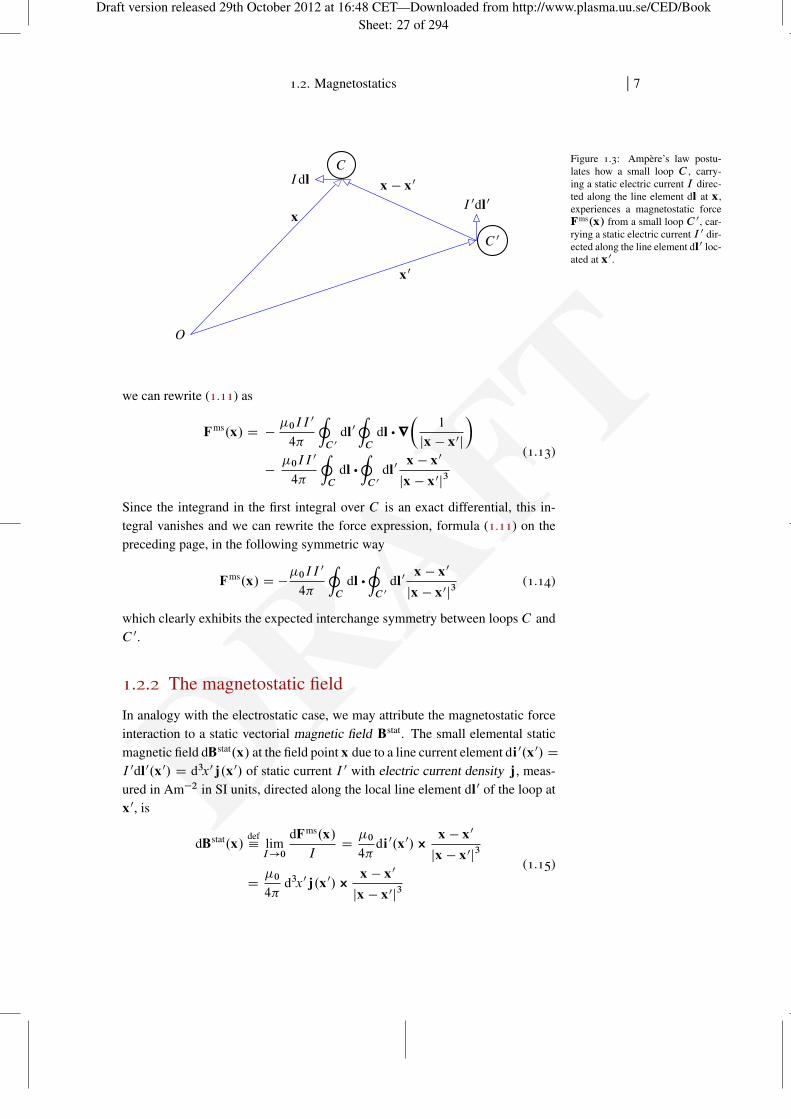
Experiments on the force interaction between two small loops that carry staticelectric currents I and I 0 (i.e. the currents I and I 0 do not vary in time) haveshown that the loops interact via a mechanical force, much the same way thatstatic electric charges interact. Let Fms.x/ denote the magnetostatic force ona loop C , with tangential line vector element dl, located at x and carrying acurrent I in the direction of dl, due to the presence of a loop C 0, with tangentialline element dl0, located at x0 and carrying a current I 0 in the direction of dl0

in otherwise empty space. This spatial configuration is illustrated in graphicalform in figure 1.3 on the facing page.

According to Ampère’s law the magnetostatic force in question is given bythe expression11

11 ANDRÉ-MARIE AMPÈRE(1775–1836) was a French math-ematician and physicist who,only a few days after he learnedabout the findings by the Danishphysicist and chemist HANSCHRISTIAN ØRSTED (1777–1851) regarding the magneticeffects of electric currents, presen-ted a paper to the Académie desSciences in Paris, postulating theforce law that now bears his name.

Fms.x/ D�0II

0

4�

IC

dl �

IC 0

dl0 �x � x0

jx � x0j3

D ��0II

0

4�

IC

dl �

IC 0

dl0 � r

�1

jx � x0j

� (1.11)

In SI units, �0 D 4� �10�7 Henry per metre (Hm�1) is the permeability of freespace . From the definition of "0 and �0 (in SI units) we observe that

"0�0 D107

4�c2(Fm�1) � 4� � 10�7 (Hm�1) D

1

c2(s2m�2) (1.12)

which is a most useful relation.At first glance, equation (1.11) above may appear asymmetric in terms of the

loops and therefore be a force law that does not obey Newton’s third law. How-ever, by applying the vector triple product ‘bac-cab’ formula (F.53) on page 216,


DRAFT

1.2. Magnetostatics j 7

C 0

C

I 0dl0

Idl

O

x0

x � x0

x

Figure 1.3: Ampère’s law postu-lates how a small loop C , carry-ing a static electric current I direc-ted along the line element dl at x,experiences a magnetostatic forceFms.x/ from a small loop C 0, car-rying a static electric current I 0 dir-ected along the line element dl0 loc-ated at x0.

we can rewrite (1.11) as

Fms.x/ D ��0II

0

4�

IC 0

dl0IC

dl � r

�1

jx � x0j

��0II

0

4�

IC

dl �

IC 0

dl0x � x0

jx � x0j3

(1.13)

Since the integrand in the first integral over C is an exact differential, this in-tegral vanishes and we can rewrite the force expression, formula (1.11) on thepreceding page, in the following symmetric way

Fms.x/ D ��0II

0

4�

IC

dl �

IC 0

dl0x � x0

jx � x0j3(1.14)

which clearly exhibits the expected interchange symmetry between loops C andC 0.

1.2.2 The magnetostatic field

In analogy with the electrostatic case, we may attribute the magnetostatic forceinteraction to a static vectorial magnetic field Bstat. The small elemental staticmagnetic field dBstat.x/ at the field point x due to a line current element di0.x0/ D

I 0dl0.x0/ D d3x0j.x0/ of static current I 0 with electric current density j, meas-ured in Am�2 in SI units, directed along the local line element dl0 of the loop atx0, is

dBstat.x/def� limI!0

dFms.x/

ID�0

4�di0.x0/ �

x � x0

jx � x0j3

D�0

4�d3x0j.x0/ �

x � x0

jx � x0j3

(1.15)


DRAFT


which is the differential form of the Biot-Savart law.The elemental field vector dBstat.x/ at the field point x is perpendicular to

the plane spanned by the line current element vector di0.x0/ at the source pointx0, and the relative position vector x � x0. The corresponding local elementalforce dFms.x/ is directed perpendicular to the local plane spanned by dBstat.x/

and the line current element di.x/. The SI unit for the magnetic field, sometimescalled the magnetic flux density or magnetic induction , is Tesla (T).

If we integrate expression (1.15) on the preceding page around the entireloop at x, we obtain

Bstat.x/ D

ZdBstat.x/

D�0

4�

ZV 0

d3x0 j.x0/ �x � x0

jx � x0j3

D ��0

4�

ZV 0

d3x0 j.x0/ � r�

1

jx � x0j

�D�0

4�r �

ZV 0

d3x0j.x0/

jx � x0j

(1.16)

where we used formula (F.114) on page 218, formula (F.87) on page 217, andthe fact that j.x0/ does not depend on the unprimed coordinates on which roperates. Comparing equation (1.7) on page 4 with equation (1.16) above, wesee that there exists an analogy between the expressions for Estat and Bstat butthat they differ in their vectorial characteristics. With this definition of Bstat,equation (1.11) on page 6 may be written

Fms.x/ D I

IC

dl � Bstat.x/ D

IC

di � Bstat.x/ (1.17)

In order to assess the properties of Bstat, we determine its divergence andcurl. Taking the divergence of both sides of equation (1.16) above and utilisingformula (F.99) on page 218, we obtain

r �Bstat.x/ D�0

4�r �r �

ZV 0

d3x0j.x0/

jx � x0jD 0 (1.18)

since, according to formula (F.99) on page 218, r �.r � a/ vanishes for anyvector field a.x/.

With the use of formula (F.128) on page 220, the curl of equation (1.16)above can be written

r � Bstat.x/ D�0

4�r � r �

ZV 0

d3x0j.x0/

jx � x0j

D �0j.x/ ��0

4�

ZV 0

d3x0 Œr 0 � j.x0/�r 0�

1

jx � x0j

� (1.19)


DRAFT

1.3. Electrodynamics j 9

assuming that j.x0/ falls off sufficiently fast at large distances. For the stationarycurrents of magnetostatics, r � j D 0 since there cannot be any charge accumu-lation in space. Hence, the last integral vanishes and we can conclude that

r � Bstat.x/ D �0j.x/ (1.20)

We se that the static magnetic field Bstat is purely rotational .

1.3 Electrodynamics

As we saw in the previous sections, the laws of electrostatics and magnetostaticscan be summarised in two pairs of time-independent, uncoupled partial differen-tial equations, namely the equations of classical electrostatics

r �Estat.x/ D�.x/

"0(1.21a)

r � Estat.x/ D 0 (1.21b)

and the equations of classical magnetostatics

r �Bstat.x/ D 0 (1.21c)

r � Bstat.x/ D �0j.x/ (1.21d)

Since there is nothing a priori that connects Estat directly with Bstat, we mustconsider classical electrostatics and classical magnetostatics as two separate andmutually independent physical theories.

However, when we include time-dependence, these theories are unified intoClassical Electrodynamics . This unification of the theories of electricity andmagnetism can be inferred from two empirically established facts:

1. Electric charge is a conserved quantity and electric current is a transport ofelectric charge. As we shall see, this fact manifests itself in the equation ofcontinuity and, as a consequence, in Maxwell’s displacement current .

2. A change in the magnetic flux through a loop will induce an electromotiveforce electric field in the loop. This is the celebrated Faraday’s law of induc-tion .


DRAFT


1.3.1 The indestructibility of electric charge

Let j.t;x/ denote the time-dependent electric current density. In the simplestcase it can be defined as j D v� where v is the velocity of the electric chargedensity �.1212 A more accurate model is to

assume that the individual chargeand current elements obey somedistribution function that describestheir local variation of velocityin space and time. For instance,j can be defined in statisticalmechanical terms as j.t;x/ DP˛ q˛

Rd3v vf˛.t;x; v/ where

f˛.t;x; v/ is the (normalised)distribution function for particlespecies ˛ carrying an electriccharge q˛ .

The electric charge conservation law can be formulated in the equation ofcontinuity for electric charge

@�.t;x/

@tC r � j.t;x/ D 0 (1.22)

or@�.t;x/

@tD �r � j.t;x/ (1.23)

which states that the time rate of change of electric charge �.t;x/ is balancedby a negative divergence in the electric current density j.t;x/, i.e. an influx ofcharge. Conservation laws will be studied in more detail in chapter 4.

1.3.2 Maxwell’s displacement current

We recall from the derivation of equation (1.20) on the previous page that therewe used the fact that in magnetostatics r � j.x/ D 0. In the case of non-stationary sources and fields, we must, in accordance with the continuity equa-tion (1.22) above, set r � j.t;x/ D �@�.t;x/=@t . Doing so, and formally re-peating the steps in the derivation of equation (1.20) on the previous page, wewould obtain the result

r � B.t;x/ D �0j.t;x/C�0

4�

ZV 0

d3x0@�.t;x0/

@tr 0�

1

jx � x0j

�(1.24)

If we assume that equation (1.7) on page 4 can be generalised to time-varyingfields, we can make the identification1313 Later, we will need to consider

this generalisation and formalidentification further. 1

4�"0

@

@t

ZV 0

d3x0 �.t;x0/r 0�

1

jx � x0j

�D

@

@t

��

1

4�"0

ZV 0

d3x0 �.t;x0/r�

1

jx � x0j

��D

@

@t

��

1

4�"0r

ZV 0

d3x0�.t;x0/

jx � x0j

�D

@

@tE.t;x/

(1.25)

The result is Maxwell’s source equation for the B field

r � B.t;x/ D �0

�j.t;x/C

@

@t"0E.t;x/

�D �0j.t;x/C �0"0

@

@tE.t;x/

(1.26)


DRAFT


where "[email protected];x/=@t is the famous displacement current . This, at the time, un-observed current was introduced by Maxwell, in a stroke of genius, in order tomake also the right-hand side of this equation divergence-free when j.t;x/ isassumed to represent the density of the total electric current. This total currentcan be split up into ‘ordinary’ conduction currents, polarisation currents andmagnetisation currents. This will be discussed in subsection 9.1 on page 188.

The displacement current behaves like a current density flowing in free space.As we shall see later, its existence has far-reaching physical consequences as itpredicts that such physical observables as electromagnetic energy, linear mo-mentum, and angular momentum can be transmitted over very long distances,even through empty space.

1.3.3 Electromotive force

If an electric field E.t;x/ is applied to a conducting medium, a current densityj.t;x/ will be set up in this medium. But also mechanical, hydrodynamicaland chemical processes can give rise to electric currents. Under certain physicalconditions, and for certain materials, one can assume that a linear relationshipexists between the electric current density j and E. This approximation is calledOhm’s law:14 14 In semiconductors this approx-

imation is in general applicableonly for a limited range of E. Thisproperty is used in semiconductordiodes for rectifying alternatingcurrents.

j.t;x/ D �E.t;x/ (1.27)

where � is the electric conductivity measured in Siemens per metre (Sm�1).We can view Ohm’s law equation (1.27) as the first term in a Taylor ex-

pansion of a general law jŒE.t;x/�. This general law incorporates non-lineareffects such as frequency mixing and frequency conversion . Examples of mediathat are highly non-linear are semiconductors and plasma. We draw the atten-tion to the fact that even in cases when the linear relation between E and j isa good approximation, we still have to use Ohm’s law with care. The conduct-ivity � is, in general, time-dependent (temporal dispersive media) but then it isoften the case that equation (1.27) above is valid for each individual temporalFourier (spectral) component of the field. In some media, such as magnetisedplasma and certain material, the conductivity is different in different directions.For such electromagnetically anisotropic media (spatial dispersive media) thescalar electric conductivity � in Ohm’s law equation (1.27) has to be replacedby a conductivity tensor . If the response of the medium is not only anisotropicbut also non-linear, higher-order tensorial terms have to be included.

If the current is caused by an applied electric field E.t;x/, this electric fieldwill exert work on the charges in the medium and, unless the medium is super-conducting, there will be some energy loss. The time rate at which this energy is


DRAFT


expended is j �E per unit volume (Wm�3). If E is irrotational (conservative), j

will decay away with time. Stationary currents therefore require that an electricfield due to an electromotive force (EMF ) is present. In the presence of such afield Eemf, Ohm’s law, equation (1.27) on the previous page, takes the form

j D �.EstatC Eemf/ (1.28)

The electromotive force is defined as

E DIC

dl �.EstatC Eemf/ (1.29)

where dl is a tangential line element of the closed loop C .1515 The term ‘electromotive force’is something of a misnomer sinceE represents a voltage, i.e. its SIdimension is V. 1.3.4 Faraday’s law of induction

In subsection 1.1.2 we derived the differential equations for the electrostaticfield. Specifically, on page 5 we derived equation (1.9b) stating thatr�Estat D 0

and hence that Estat is a conservative field (it can be expressed as a gradient of ascalar field). This implies that the closed line integral of Estat in equation (1.29)above vanishes and that this equation becomes

E DIC

dl �Eemf (1.30)

It has been established experimentally that a non-conservative EMF field isproduced in a closed circuit C at rest if the magnetic flux through this circuitvaries with time. This is formulated in Faraday’s law which, in Maxwell’s gen-eralised form, reads

E.t/ DIC

dl �E.t;x/ D �ddtˆm.t/

D �ddt

ZS

d2x On �B.t;x/ D �ZS

d2x On �@

@tB.t;x/

(1.31)

where ˆm is the magnetic flux and S is the surface encircled by C , interpretedas a generic stationary ‘loop’ and not necessarily as a conducting circuit. Ap-plication of Stokes’ theorem on this integral equation, transforms it into the dif-ferential equation

r � E.t;x/ D �@

@tB.t;x/ (1.32)

that is valid for arbitrary variations in the fields and constitutes the Maxwellequation which explicitly connects electricity with magnetism.

Any change of the magnetic flux ˆm will induce an EMF. Let us thereforeconsider the case, illustrated in figure 1.4 on the facing page, when the ‘loop’ is


DRAFT


d2x On

B.x/ B.x/

v

dl

C

Figure 1.4: A loop C that moveswith velocity v in a spatially vary-ing magnetic field B.x/ will sensea varying magnetic flux during themotion.

moved in such a way that it encircles a magnetic field which varies during themovement. The total time derivative is evaluated according to the well-knownoperator formula

ddtD

@

@tC

dx

dt� r (1.33)

This follows immediately from the multivariate chain rule for the differentiationof an arbitrary differentiable function f .t;x.t//. Here, dx=dt describes a chosenpath in space. We shall choose the flow path which means that dx=dt D v and

ddtD

@

@tC v � r (1.34)

where, in a continuum picture, v is the fluid velocity. For this particular choice,the convective derivative dx=dt is usually referred to as the material derivativeand is denoted Dx=Dt .

Applying the rule (1.34) to Faraday’s law, equation (1.31) on the precedingpage, we obtain

E.t/ D �ddt

ZS

d2x On �B D �ZS

d2x On �@B

@t�

ZS

d2x On � .v � r /B (1.35)

Furthermore, taking the divergence of equation (1.32) on the facing page, we seethat

r �@

@tB.t;x/ D

@

@tr �B.t;x/ D �r �Œr � E.t;x/� D 0 (1.36)

where in the last step formula (F.99) on page 218 was used. Since this is true forall times t , we conclude that

r �B.t;x/ D 0 (1.37)


DRAFT


also for time-varying fields; this is in fact one of the Maxwell equations. Usingthis result and formula (F.89) on page 217, we find that

r � .B � v/ D .v � r /B (1.38)

since, during spatial differentiation, v is to be considered as constant, This allowsus to rewrite equation (1.35) on the previous page in the following way:

E.t/ DIC

dl �EemfD �

ddt

ZS

d2x On �B

D �

ZS

d2x On �@B

@t�

ZS

d2x On � r � .B � v/

(1.39)

With Stokes’ theorem applied to the last integral, we finally get

E.t/ DIC

dl �EemfD �

ZS

d2x On �@B

@t�

IC

dl �.B � v/ (1.40)

or, rearranging the terms,IC

dl �.Eemf� v � B/ D �

ZS

d2x On �@B

@t(1.41)

where Eemf is the field induced in the ‘loop’, i.e. in the moving system. Theapplication of Stokes’ theorem ‘in reverse’ on equation (1.41) above yields

r � .Eemf� v � B/ D �

@B

@t(1.42)

An observer in a fixed frame of reference measures the electric field

E D Eemf� v � B (1.43)

and an observer in the moving frame of reference measures the following Lorentzforce on a charge q

F D qEemfD qEC q.v � B/ (1.44)

corresponding to an ‘effective’ electric field in the ‘loop’ (moving observer)

EemfD EC v � B (1.45)

Hence, we conclude that for a stationary observer, the Maxwell equation

r � E D �@B

@t(1.46)

is indeed valid even if the ‘loop’ is moving.


DRAFT


1.3.5 The microscopic Maxwell equations

We are now able to collect the results from the above considerations and formu-late the equations of classical electrodynamics, valid for arbitrary variations intime and space of the coupled electric and magnetic fields E.t;x/ and B.t;x/.The equations are, in SI units ,16 16 In CGS units the Maxwell-

Lorentz equations are

r �E D 4��

r �B D 0

r �EC1

c

@B

@tD 0

r �B �1

c

@E

@tD4�

cj

in Heaviside-Lorentz units (one ofseveral natural units)

r �E D �

r �B D 0

r �EC1

c

@B

@tD 0

r �B �1

c

@E

@tD1

cj

and in Planck units (another set ofnatural units)

r �E D 4��

r �B D 0

r �EC@B

@tD 0

r �B �@E

@tD 4�j

r �E D�

"0(1.47a)

r �B D 0 (1.47b)

r � EC@B

@tD 0 (1.47c)

r � B �1

c2@E

@tD �0j (1.47d)

In these equations � D �.t;x/ represents the total, possibly both time and spacedependent, electric charge density, with contributions from free as well as in-duced (polarisation) charges. Likewise, j D j.t;x/ represents the total, possiblyboth time and space dependent, electric current density, with contributions fromconduction currents (motion of free charges) as well as all atomistic (polarisationand magnetisation) currents. As they stand, the equations therefore incorporatethe classical interaction between all electric charges and currents, free or bound,in the system and are called Maxwell’s microscopic equations . They were firstformulated by Lorentz and therefore another name frequently used for them isthe Maxwell-Lorentz equations and the name we shall use. Together with theappropriate constitutive relations that relate � and j to the fields, and the initialand boundary conditions pertinent to the physical situation at hand, they form asystem of well-posed partial differential equations that completely determine E

and B.

1.3.6 Dirac’s symmetrised Maxwell equations

If we look more closely at the microscopic Maxwell equations (1.47), we seethat they exhibit a certain, albeit not complete, symmetry. Dirac therefore madethe ad hoc assumption that there exist magnetic monopoles represented by amagnetic charge density, which we denote by �m D �m.t;x/, and a magneticcurrent density, which we denote by jm D jm.t;x/.17

17 JULIAN SEYMOURSCHWINGER (1918–1994)once put it:

‘. . . there are strong theor-etical reasons to believethat magnetic charge existsin nature, and may haveplayed an important rolein the development ofthe Universe. Searchesfor magnetic charge con-tinue at the present time,emphasising that electro-magnetism is very far frombeing a closed object’.

The magnetic monopole was firstpostulated by P IERRE CURIE(1859–1906) and inferred fromexperiments in 2009.

With these new hypothetical physical entities included in the theory, and withthe electric charge density denoted �e and the electric current density denotedje, the Maxwell-Lorentz equations will be symmetrised into the following two


DRAFT


scalar and two coupled vectorial partial differential equations (SI units):

r �E D�e

"0(1.48a)

r �B D �0�m (1.48b)

r � EC@B

@tD ��0j

m (1.48c)

r � B �1

c2@E

@tD �0j

e (1.48d)

We shall call these equations Dirac’s symmetrised Maxwell equations or theelectromagnetodynamic equations .

Taking the divergence of (1.48c), we find that

r �.r � E/ D �@

@t.r �B/ � �0r � j

m� 0 (1.49)

where we used the fact that the divergence of a curl always vanishes. Using(1.48b) to rewrite this relation, we obtain the equation of continuity for magneticcharge

@�m

@tC r � jm

D 0 (1.50)

which has the same form as that for the electric charges (electric monopoles) andcurrents, equation (1.22) on page 10.

1.4 Examples

BFaraday’s law derived from the assumed conservation of magnetic chargeEXAMPLE 1 .1

POSTULATE 1.1 (INDESTRUCTIBILITY OF MAGNETIC CHARGE) Magnetic charge ex-ists and is indestructible in the same way that electric charge exists and is indestructible.

In other words, we postulate that there exists an equation of continuity for magnetic charges:

@�m.t;x/

@tC r � jm.t;x/ D 0 (1.51)

Use this postulate and Dirac’s symmetrised form of Maxwell’s equations to derive Faraday’slaw.

The assumption of the existence of magnetic charges suggests a Coulomb-like law for mag-


DRAFT

1.4. Examples j 17

netic fields:

Bstat.x/ D�0

4�

ZV 0

d3x0 �m.x0/x � x0

jx � x0j3D �

�0

4�

ZV 0

d3x0 �m.x0/r

�1

jx � x0j

�D �

�0

4�r

ZV 0

d3x0�m.x0/

jx � x0j

(1.52)

[cf. equation (1.7) on page 4 for Estat] and, if magnetic currents exist, a Biot-Savart-likelaw for electric fields [cf. equation (1.16) on page 8 for Bstat]:

Estat.x/ D ��0

4�

ZV 0

d3x0 jm.x0/ �x � x0

jx � x0j3D�0

4�

ZV 0

d3x0 jm.x0/ � r

�1

jx � x0j

�D �

�0

4�r �

ZV 0

d3x0jm.x0/

jx � x0j

(1.53)

Taking the curl of the latter and using formula (F.128) on page 220

r � Estat.x/ D ��0jm.x/ ��0

4�

ZV 0

d3x0 Œr 0 � jm.x0/�r 0�

1

jx � x0j

�(1.54)

assuming that jm falls off sufficiently fast at large distances. Stationarity means thatr � jm D 0 so the last integral vanishes and we can conclude that

r � Estat.x/ D ��0jm.x/ (1.55)

It is intriguing to note that if we assume that formula (1.53) above is valid also for time-varying magnetic currents, then, with the use of the representation of the Dirac delta func-tion, equation (F.116) on page 218, the equation of continuity for magnetic charge, equation(1.50) on the preceding page, and the assumption of the generalisation of equation (1.52)above to time-dependent magnetic charge distributions, we obtain, at least formally,

r � E.t;x/ D ��0jm.t;x/ �@

@tB.t;x/ (1.56)

[cf. equation (1.24) on page 10] which we recognise as equation (1.48c) on the facing page.A transformation of this electromagnetodynamic result by rotating into the ‘electric realm’of charge space, thereby letting jm tend to zero, yields the electrodynamic equation (1.47c)on page 15, i.e. the Faraday law in the ordinary Maxwell equations. This process would alsoprovide an alternative interpretation of the term @B=@t as a magnetic displacement current ,dual to the electric displacement current [cf. equation (1.26) on page 10].

By postulating the indestructibility of a hypothetical magnetic charge, and assuming a dir-ect extension of results from statics to dynamics, we have been able to replace Faraday’sexperimental results on electromotive forces and induction in loops as a foundation for theMaxwell equations by a more fundamental one. At first sight, this result seems to be inconflict with the concept of retardation. Therefore a more detailed analysis of it is required.This analysis is left to the reader.

End of example 1.1C


DRAFT


1.5 Bibliography

[1] T. W. BARRETT AND D. M. GRIMES, Advanced Electromagnetism. Founda-tions, Theory and Applications, World Scientific Publishing Co., Singapore, 1995,ISBN 981-02-2095-2.

[2] R. BECKER, Electromagnetic Fields and Interactions, Dover Publications, Inc.,New York, NY, 1982, ISBN 0-486-64290-9.

[3] W. GREINER, Classical Electrodynamics, Springer-Verlag, New York, Berlin,Heidelberg, 1996, ISBN 0-387-94799-X.

[4] E. HALLÉN, Electromagnetic Theory, Chapman & Hall, Ltd., London, 1962.

[5] K. HUANG, Fundamental Forces of Nature. The Story of Gauge Fields, World Sci-entific Publishing Co. Pte. Ltd, New Jersey, London, Singapore, Beijing, Shanghai,Hong Kong, Taipei, and Chennai, 2007, ISBN 13-978-981-250-654-4 (pbk).

[6] J. D. JACKSON, Classical Electrodynamics, third ed., John Wiley & Sons, Inc.,New York, NY . . . , 1999, ISBN 0-471-30932-X.

[7] L. D. LANDAU AND E. M. LIFSHITZ, The Classical Theory of Fields, fourth re-vised English ed., vol. 2 of Course of Theoretical Physics, Pergamon Press, Ltd.,Oxford . . . , 1975, ISBN 0-08-025072-6.

[8] F. E. LOW, Classical Field Theory, John Wiley & Sons, Inc., New York, NY . . . ,1997, ISBN 0-471-59551-9.

[9] J. C. MAXWELL, A Treatise on Electricity and Magnetism, third ed., vol. 1, DoverPublications, Inc., New York, NY, 1954, ISBN 0-486-60636-8.

[10] J. C. MAXWELL, A Treatise on Electricity and Magnetism, third ed., vol. 2, DoverPublications, Inc., New York, NY, 1954, ISBN 0-486-60637-8.

[11] D. B. MELROSE AND R. C. MCPHEDRAN, Electromagnetic Processes in DispersiveMedia, Cambridge University Press, Cambridge . . . , 1991, ISBN 0-521-41025-8.

[12] W. K. H. PANOFSKY AND M. PHILLIPS, Classical Electricity and Magnetism,second ed., Addison-Wesley Publishing Company, Inc., Reading, MA . . . , 1962,ISBN 0-201-05702-6.

[13] F. ROHRLICH, Classical Charged Particles, third ed., World Scientific PublishingCo. Pte. Ltd., New Jersey, London, Singapore, . . . , 2007, ISBN 0-201-48300-9.

[14] J. A. STRATTON, Electromagnetic Theory, McGraw-Hill Book Company, Inc., NewYork, NY and London, 1953, ISBN 07-062150-0.

[15] J. VANDERLINDE, Classical Electromagnetic Theory, John Wiley & Sons, Inc., NewYork, Chichester, Brisbane, Toronto, and Singapore, 1993, ISBN 0-471-57269-1.


DRAFT2

ELECTROMAGNETIC FIELDS AND

WAVES

As a first step in the study of the dynamical properties of the classical elec-tromagnetic field, we shall in this chapter, as an alternative to the first-orderMaxwell-Lorentz equations, derive a set of second-order differential equationsfor the fields E and B. It turns out that these second-order equations are waveequations for the field vectors E and B, indicating that electromagnetic vectorwave modes are very natural and common manifestations of classical electro-dynamics.1 1 In 1864, in a lecture at the

Royal Society of London, JAMESCLERK MAXWELL (1831–1879)himself said:

‘We have strong reason toconclude that light itself— including radiant heatand other radiation, if any— is an electromagneticdisturbance in the form ofwaves propagated throughthe electro-magnetic fieldaccording to electro-magnetic laws.’

But before deriving these alternatives to the Maxwell-Lorentz equations, weshall discuss the mathematical techniques of making use of complex variables torepresent physical observables in order to simplify the mathematical treatment.In this chapter we will also describe how to make use of the single spectralcomponent (Fourier component) technique, which simplifies the algebra, at thesame time as it clarifies the physical content.

2.1 Axiomatic classical electrodynamics

In chapter 1 we described the historical route which led to the formulation of themicroscopic Maxwell equations. From now on we shall consider these equationsas postulates , i.e. as the axiomatic foundation of classical electrodynamics .2 As 2 FRITZ ROHRLICH writes in

Classical Charged Particles that

‘A physical theory, inthe narrow sense of theword, is a logical structurebased on assumptions anddefinitions which permitsone to predict the outcomeof a maximum number ofdifferent experiments onthe basis of a minimumnumber of postulates.One usually desires thepostulates (or axioms) to beas self-evident as possible;one demands simplicity,beauty, and even elegance.’

such, these equations postulate, in scalar and vector differential equation form,the behaviour in time t 2 R and in space x 2 R3 of the relation between theelectric and magnetic fields E.t;x/ 2 R3 and B.t;x/ 2 R3, respectively, andthe charge density �.t;x/ 2 R and current density j.t;x/ 2 R3 [cf. equations(1.47) on page 15]

r �E D�

"0(Gauss’s law) (2.1a)

r �B D 0 (No magnetic charges) (2.1b)

r � EC@B

@tD 0 (Faraday’s law) (2.1c)

r � B �1

c2@E

@tD �0j (Maxwell’s law) (2.1d)

19


DRAFT

20 j 2. ELECTROMAGNETIC FIELDS AND WAVES

and are not to be viewed as equations that only describe how the fields E and B

are generated by � and j, but also the other way around.We reiterate that in these equations �.t;x/ and j.t;x/ are the total charge

and current densities, respectively. Hence, these equations are considered mi-croscopic in the sense that all charges and currents, including the intrinsic onesin matter, such as bound charges in atoms and molecules as well as magnetisa-tion currents in magnetic material, are included, but macroscopic in the sensethat quantum effects are neglected. Despite the fact that the charge and cur-rent densities may not only be considered as the sources of the fields, but mayequally well be considered being generated by the fields, we shall follow theconvention and refer to them as the source terms of the microscopic Maxwellequations. Analogously, the two equations where they appear will be referred toas the Maxwell-Lorentz source equations .

I we allow for magnetic charge and current densities �m and jm, respect-ively, in addition to electric charge and current densities �e � � and je � j,we will have to replace the Maxwell-Lorentz equations by Dirac’s symmetrisedequations

r �E D�e

"0(2.2a)

r �B D �0�mD

�m

c2"0(2.2b)

r � EC@B

@tD ��0j

m (2.2c)

r � B �1

c2@E

@tD �0j

e (2.2d)

and consider them to be the postulates of electromagnetodynamics.

2.2 Complex notation and physical observables

In order to simplify the mathematical treatment, we shall frequently allow themathematical variables that represent the fields, the charge and current densities,and other physical quantities be analytically continued into the complex domain.However, when we use such a complex notation we must be very careful howto interpret the results derived within this notation. This is because every phys-ical observable is, by definition, real-valued.3 Consequently, the mathematical

3 A physical observable is some-thing that can, one way or another,be ultimately reduced to an inputto the human sensory system. Inother words, physical observablesquantify (our perception of) thephysical reality and as such theymust, of course, be described byreal-valued quantities.

expression for the observable under consideration must also be real-valued to bephysically meaningful.

If a physical scalar variable, or a component of a physical vector or tensor,is represented mathematically by the complex-valued number , i.e. if 2 C,


DRAFT

2.2. Complex notation and physical observables j 21

then in classical electrodynamics (in fact, in classical physics as a whole), onemakes the identification observable D Re

˚ mathematical

. Therefore, it is always

understood that one must take the real part of a complex mathematical variablein order for it to represent a classical physical observable, i.e. something that isobserved in Nature or measured in an experiment.4 4 This is at variance with

quantum physics, where observable D

ˇ̌ mathematical

ˇ̌.

Letting � denote complex conjug-ation, the real part can be writtenRe f g D 1

2. C �/, i.e. as

the arithmetic mean of and itscomplex conjugate �. Similarly,the magnitude can be writtenj j D . �/1=2, i.e. as thegeometric mean of and �.Under certain conditions, also theimaginary part corresponds to aphysical observable.

For mathematical convenience and ease of calculation, we shall in the fol-lowing regularly use — and tacitly assume — complex notation, stating ex-plicitly when we do not. One convenient property of the complex notation isthat differentiations often become trivial to perform. However, care must al-ways be exercised. A typical situation being when products of two or morequantities are calculated since, for instance, for two complex-valued variables 1 and 2 we know that Re f 1 2g ¤ Re f 1gRe f 2g. On the other hand,. 1 2/

�D 1

� 2�.

2.2.1 Physical observables and averages

As just mentioned, it is important to be aware of the limitations of the math-ematical technique of using a complex representation for physical observables,particularly when evaluating products of complex mathematical variables thatare to represent physical observables.

Let us, for example, consider two physical vector fields a.t;x/ and b.t;x/

represented by their Fourier components a0.x/ exp.�i!t/ and b0.x/ exp.�i!t/,i.e. by vectors in (a domain of) 3D complex space C3. Furthermore, let ı be abinary infix operator for these vectors, representing either the scalar productoperator �, the vector product operator �, or the dyadic product operator . Toensure that any products of a and b represent an observable in classical physics,we must make the interpretation

a.t;x/ ıb.t;x/ � Re fag ıRe fbg

D Re˚a0.x/ e�i!t

ıRe˚b0.x/ e�i!t (2.3)

We can express the real part of the complex vectors a and b as

Re fag D Re˚a0.x/ e�i!t

D1

2Œa0.x/ e�i!t

C a0�.x/ ei!t � (2.4a)

and

Re fbg D Re˚b0.x/ e�i!t

D1

2Œb0.x/ e�i!t

C b0�.x/ ei!t � (2.4b)

respectively. Hence, the physically acceptable interpretation of the scalar product


DRAFT


of two complex vectors, representing classical physical observables, is

a.t;x/ ıb.t;x/ D Re˚a0.x/ e�i!t

ıRe˚b0.x/ e�i!t

D1

2Œa0.x/ e�i!t

C a0�.x/ ei!t � ı

1

2Œb0.x/ e�i!t

C b0�.x/ ei!t �

D1

4

�a0 ıb0

�C a0

�ıb0 C a0 ıb0 e�2i!t

C a0�ıb0

� e2i!t�D1

2Re fa0 ıb0

�g C

1

2Re˚a0 ıb0 e�2i!t

D1

2Re˚a0 e�i!t

ıb0� ei!t

C1

2Re˚a0e�i!t

ıb0 e�i!tD1

2Re fa.t;x/ ıb�.t;x/g C

1

2Re fa.t;x/ ıb.t;x/g

(2.5)

In physics, we are often forced to measure the temporal average (cycle aver-age) of a physical observable. We use the notation h� � �it for such an average andfind that the average of the product of the two physical quantities represented bya and b can be expressed as

ha ıbit � hRe fag ıRe fbgit D1

2Re fa ıb�g D

1

2Re fa� ıbg

D1

2Re fa0 ıb0

�g D

1

2Re fa0� ıb0g

(2.6)

This is because the oscillating function exp.�2i!t/ in equation (2.5) above van-ishes when averaged in time over a complete cycle 2�=! (or over infinitely manycycles), and, therefore, ha.t;x/ ıb.t;x/it gives no contribution.

2.2.2 Maxwell equations in Majorana representation

It is often convenient to express electrodynamics in terms of the complex-fieldsix-vector , also known as the Riemann-Silberstein vector ,

G.t;x/ D E.t;x/C icB.t;x/ (2.7)

where G 2 C3 even if E;B 2 R3. If we use this vector, the Maxwell equations(2.1) on page 19 can be written

r �G D�

"0(2.8a)

r �G �ic

@G

@tD ic�0j (2.8b)

In regions where � D 0 and j D 0 these equations reduce to

r �G D 0 (2.9a)

r �G Dic

@G

@t(2.9b)


DRAFT

2.3. The wave equations for E and B j 23

which, with the help of the linear momentum operator

yp D �i}r (2.10)

can be rewritten

yp �G D 0 (2.11a)

i}@G

@tD ciyp �G (2.11b)

The first equation is the transversality condition p D }k ? G where we anti-cipate the usual quantal relation between the field momentum p and the wavevector k,5 whereas the second equation describes the dynamics. 5 The scalar quantity } D h=.2�/

is the reduced Planck constantwhere the Planck constant properh � 6:62606957� 10�34 Js.

Using formula (F.105) on page 218, we can rewrite equation (2.11b) aboveas

i}@G

@tD c.S � yp/G (2.12)

where

S D

0B@0 0 0

0 0 �i0 i 0

1CA Ox1 C0B@ 0 0 i0 0 0

�i 0 0

1CA Ox2 C0B@0 �i 0

i 0 0

0 0 0

1CA Ox3 (2.13)

Then by introducing the Hamiltonian-like operator

yH D cS � yp D �ic}S � r (2.14)

we can write the Maxwell-Lorentz curl equations as

i}@G

@tD yHG (2.15)

i.e. as a Schrödinger/Pauli/Dirac-like equation; sometimes these are referredto as neutrino equations . This formulation of the free-space electromagneticfield equations is known as the Majorana representation of the Maxwell-Lorentzequations or the Majorana formalism .6

6 It so happens that ETTOREMAJORANA (1906-1938) used thedefinition G D E � icB, but thisis no essential difference from thedefinition (2.7). One may say thatMajorana used the other branch ofp�1 as the imaginary unit.

2.3 The wave equations for E and B

The Maxwell-Lorentz equations (2.1) on page 19 are four first-order coupleddifferential equations (both E and B appear in the same equations). Two of theequations are scalar [equations (2.1a) and (2.1b)], and two are in 3D Euclideanvector form [equations (2.1c) and (2.1d)], representing three scalar equations


DRAFT


each. Hence, the Maxwell equations represent eight (1C 1C 3C 3 D 8) scalarcoupled first-order partial differential equations. However, it is well known fromthe theory of differential equations that a set of first-order, coupled partial dif-ferential equations can be transformed into a smaller set of second-order partialdifferential equations that sometimes become decoupled in the process. It turnsout that in our case we will obtain one second-order differential equation forE and one second-order differential equation for B. These second-order partialdifferential equations are, as we shall see, wave equations , and we shall discusstheir properties and implications. In certain propagation media, the B wave fieldcan be easily obtained from the solution of the E wave equation but in generalthis is not the case.

To bring the first-order differential equations (2.1) on page 19 into second or-der one needs, of course, to operate on them with first-order differential operat-ors. If we apply the curl vector operator (r�) to both sides of the two Maxwell-Lorentz vector equations (2.1c) and (2.1d) on page 19, assuming that the fieldsvary in such a regular way that temporal and spatial differentiation commute, weobtain the second-order differential equations

r � .r � E/C r �@B

@tD r � .r � E/C

@

@t.r � B/ D 0 (2.16a)

r � .r � B/ �1

c2@

@t.r � E/ D �0r � j (2.16b)

As they stand, these second-order partial differential equations still appear to becoupled. However, by using the Maxwell-Lorentz equations (2.1) on page 19once again we can formally decouple them into

1

c2@2E

@t2C r � .r � E/ D ��0

@j

@t(2.17a)

1

c2@2B

@t2C r � .r � B/ D �0r � j (2.17b)

If we use the operator triple product ‘bac-cab’ formula (F.96) on page 218, whichgives

r � .r � E/ D r .r �E/ � r2E (2.18)

when applied to E and similarly to B, Gauss’s law equation (2.1a) on page 19,and then rearrange the terms, we obtain the two inhomogeneous vector waveequations

1

c2@2E

@t2� r

2E D �2E D �r�

"0� �0

@j

@t(2.19a)

1

c2@2B

@t2� r

2B D �2B D �0r � j (2.19b)


DRAFT


where�2 is the d’Alembert operator , defined by expression (F.182) on page 226.These are the general wave equations for the electromagnetic fields in regionswhere there exist sources �.t;x/ and j.t;x/ of any kind. Simple everyday ex-amples of such regions are electric conductors (e.g. radio and TV transmitterantennas) or plasma (e.g. the Sun and its surrounding corona). In principle, thesources � and j can still cause the wave equations to be coupled, but in manyimportant situations this is not the case.7 7 Clearly, if the current density

in the RHS (‘right-hand side’) ofequation (2.19b) is a function ofE, as is the case if, for instance,Ohm’s law j D �E is applicable,the coupling is not removed.

We notice that outside the source region, i.e. in free space where � D 0

and j D 0, the inhomogeneous wave equations (2.19) on the preceding pagesimplify to the well-known uncoupled, homogeneous wave equations

�2E D1

c2@2E

@t2� r

2E D 0 (2.20a)

�2B D1

c2@2B

@t2� r

2B D 0 (2.20b)

These equations describe how the fields that were generated in the source region,propagate as vector waves through free space. Once these waves impinge uponanother region that can sustain charges and/or currents for a long enough time,such as a receiving antenna or other electromagnetic sensors, the fields inter-act with the charges and the currents in this second region in accordance withequations (2.19) on the facing page.

2.3.1 The time-independent wave equations for E and B

Often one can assume that the temporal dependency of E and B and of thesources � and j is well-behaved enough that it can be represented by the sumof a finite number N of temporal spectral components (temporal Fourier com-ponents), or, in other words, in the form of a temporal Fourier series . In suchsituations it is sufficient to study the properties of one arbitrary member of thisset of spectral components f!n W n D 1; 2; 3; : : : ; N g, i.e.

E.t;x/ D En.x/ cos.!nt / D En.x/Re˚e�i!nt

� En.x/e�i!nt (2.21a)

B.t;x/ D Bn.x/ cos.!nt / D Bn.x/Re˚e�i!nt

� Bn.x/e�i!nt (2.21b)

where En;Bn 2 R3 and !n; t 2 R is assumed. This is because the Maxwell-Lorentz equations are linear, implying that the general solution is obtained by aweighted linear superposition (summation) of the result for each such spectralcomponent, where the weight of the spectral component in question is given byits Fourier amplitude , En.x/, and Bn.x/, respectively.

In a physical system, a temporal spectral component is identified uniquely byits angular frequency !n. A wave containing only a finite number of temporal


DRAFT


spectral components is called a time-harmonic wave . In the limit when onlyone single frequency is present, we talk about a monochromatic wave . Strictlyspeaking, purely monochromatic waves do not exist.88 When subtle classical and

quantum radiation effects are takeninto account, one finds that allemissions suffer an unavoidable,intrinsic line broadening . Also,simply because the Universe hasexisted for only about 13.5 billionyears, which is a finite time, nosignals in the Universe can beobserved to have a spectral widththat is smaller than the inverse ofthis age.

By inserting the temporal spectral component equation (2.21a) on the previ-ous page into equation (2.19a) on page 24 one finds that for an arbitrary com-ponent the following equation is obtained:

r2Ene�i!nt C

!2nc2

Ene�i!nt C i!n�0jne�i!nt Dr�n

"0e�i!nt (2.22)

After dividing out the common factor exp.�i!nt /, we obtain the time-independentwave equation

r2En C

!2nc2

En C i!n�0jn Dr�n

"0(2.23)

and similarly for B. Solving this equation, multiplying the solution obtainedby exp.�i!nt / and summing over all N such Fourier (spectral) componentswith frequencies !n; n D 1; 2; 3; : : : ; N present in the sources, and hence in thefields, the complete solution of the original wave equation is obtained. This is aconsequence of the superposition principle which is valid as long as nonlineareffects can be neglected.

In the limit of very many frequency components, the Fourier sum goes overinto a Fourier integral . To illustrate this generic case, let us introduce the Fouriertransform of E.t;x/

E!.x/ D1

2�

Z 1�1

dt E.t;x/ ei!t (2.24a)

and the corresponding inverse Fourier transform

E.t;x/ D

Z 1�1

d! E!.x/ e�i!t (2.24b)

where the amplitude E!.x/ 2 C3 is a continuous function of (angular) fre-quency ! 2 R and of x 2 R3.

We see that the Fourier transform of @E.t;x/=@t becomes

1

2�

Z 1�1

dt�@E.t;x/

@t

�ei!t

D1

2�

�E.t;x/ ei!t �1

�1„ ƒ‚ …D0 since E!0; t!˙1

�i!1

2�

Z 1�1

dt E.t;x/ ei!t

D �i! E!.x/

(2.25)

and that, consequently,

1

2�

Z 1�1

dt�@2E.t;x/

@t2

�ei!tD �!2E!.x/ (2.26)


DRAFT


Fourier transforming equation (2.19a) on page 24, and using formulæ (2.25)and (2.26) on the facing page, we thus obtain

r2E! C

!2

c2E! C i!�0j! D

r�!

"0(2.27)

which is mathematically identical to equation (2.23) on the preceding page. Asubsequent inverse Fourier transformation of the solution E! of this equationleads to the same result as is obtained from the solution of equation (2.23) onthe facing page. Hence, by considering just one temporal Fourier componentwe obtain results which are identical to those that we would have obtained byemploying the machinery of Fourier transforms and Fourier integrals. Hence,under the assumption of linearity (superposition principle) there is usually noneed for the formal forward and inverse Fourier transform technique.

What was said above in general terms about temporal spectral components istrue also for spatial spectral components (spatial Fourier components) only thatwe must use a three-dimensional Fourier representation

Ek.t/ D1

.2�/3

Z 1�1

d3x E.t;x/ e�ik �x (2.28a)

E.t;x/ D

Z 1�1

d3k Ek.t/ eik �x (2.28b)

Since we always assume that the real part shall be taken (if necessary), wecan pick any pair of the spatial amplitudes in equations (2.21a) and (2.21b) onpage 25, denote the members of this pair by E0 and B0, respectively, and thenrepresent them as the Fourier modes

E0.x/ D e0Re˚eik0 �x

D E!;keik �x (2.29a)

B0.x/ D b0Re˚eik0 �x

D B!;keik �x (2.29b)

respectively, where k0 is the wave vector (measured in m�1) of mode 0; in thelast step we introduced a complex notation and also dropped the mode numbersince the formulæ are valid for any mode n.

Now, since

@

@te�i!t

D �i!e�i!t (2.30a)

and

r eik �xD Oxi

@

@xieikj xj D iOxikj ıij eikj xj D iOxikieikj xj D ikeik �x (2.30b)

we see that for each spectral component in equations (2.29) above, temporaland spatial differential operators turn into algebraic operations according to the


DRAFT


following scheme:

@

@t7! �i! (2.31a)

r 7! ik (2.31b)

r � 7! ik � (2.31c)

r � 7! ik� (2.31d)

We note that

r �E D ik �E D ik �Ek (2.32a)

r � E D ik � E D ik � E? (2.32b)

r �B D ik �B D ik �Bk (2.32c)

r � B D ik � B D ik � B? (2.32d)

r� D ik� (2.32e)

r � j D ik � j D ik � jk (2.32f)

r � j D ik � j D ik � j? (2.32g)

Hence, with respect to the wave vector k, the r � operator projects out thespatially longitudinal component, and the r� operator projects out the spatiallytransverse component of the field vector in question. Put in another way,

r �E? D 0 (2.33a)

r � Ek D 0 (2.33b)

and so on for the other observables. This can be viewed as a instance in k spaceof the Helmholtz’s theorem , discussed in subsection M.3.7 on page 245, sayingthat if E falls off suitably rapidly at infinity, it can be written as the sum of arotational part Erotat and an irrotational part Eirrot:

E D ErotatC Eirrot (2.34)

where, according to equations (M.85) on page 246,

r �ErotatD 0 (2.35a)

r � EirrotD 0 (2.35b)

by making the formal identification9

9 Strictly speaking, the spatialFourier component is a plane waveand plane waves do not fall off atall at infinity as required for theHelmholtz decomposition to beapplicable. However, only wavepackets made up of a sum of planewaves are physically acceptableand such packages can be localisedwell enough.

E? D Erotat (2.36a)

Ek D Eirrot (2.36b)


DRAFT


For the magnetic field

B D BrotatC Birrot (2.37)

where

r �BrotatD 0 (2.38a)

r � BirrotD 0 (2.38b)

we make the analogous formal identification

B? D Brotat (2.39)

Bk D Birrot (2.40)

As we see from equations (2.31) on the preceding page, the Fourier transformof a function of time t is a function of angular frequency !, and the Fouriertransform of a function of the position vector x is a function of the wave vectork. One says that ! is a reciprocal space to t and that k spans a space that isreciprocal to x. In the reciprocal ! and k space the Maxwell-Lorentz equationsare

ik �Ek D�

"0(2.41a)

ik �Bk D 0 (2.41b)

ik � E? � i!B D 0 (2.41c)

ik � B? C i!

c2E D �0j (2.41d)

Applying the Helmholtz decomposition, the Maxwell-Lorentz equations be-come

r �EirrotD

�

"0(2.42a)

r �BirrotD 0 (2.42b)

r � ErotatC@B

@tD 0 (2.42c)

r � Brotat�1

c2@E

@tD �0j (2.42d)


DRAFT


2.4 Examples

BProducts of Riemann-Silberstein vectors with themselves for E;B 2 R3EXAMPLE 2 .1

One fundamental property of the 3D complex vector space C3, to which the Riemann-Silberstein vector G D E C icB belongs, is that inner (scalar) products in this space areinvariant under rotations just as they are in R3. However, as discussed in example M.4 onpage 253, products in C3 can be defined in two different ways. Considering the specialcase of the scalar product of G with itself, assuming that E 2 R3 and B 2 R3, we have thefollowing two possibilities:

1. The inner (scalar) product defined as G scalar multiplied with itself

G �G D .EC icB/ �.EC icB/ D E �E � c2B �BC 2icE �B (2.43)

Since ‘length’ is a scalar quantity that is invariant under rotations, we find that

E2 � c2B2 D Const (2.44a)

E �B D Const (2.44b)

2. The inner (scalar) product defined as G scalar multiplied with the complex conjugate ofitself

G �G� D .EC icB/ �.E � icB/ D E �EC c2B �B � E2 C c2B2 (2.45)

is also an invariant scalar quantity. As we shall see in chapter chapter 4, this quantity isproportional to the electromagnetic field energy density.

3. As with any 3D vector, the cross product of G with itself vanishes:

G �G D .EC icB/ � .EC icB/

D E � E � c2B � BC ic.E � B/C ic.B � E/

D 0C 0C ic.E � B/ � ic.E � B/ D 0

(2.46)

4. The cross product of G with the complex conjugate of itself does, however, not vanish.Instead it is

G �G� D .EC icB/ � .E � icB/

D E � EC c2B � B � ic.E � B/C ic.B � E/

D 0C 0 � ic.E � B/ � ic.E � B/ D �2ic.E � B/

(2.47)

which is proportional to the electromagnetic energy flux (the so called Poynting vectoror the electromagnetic linear momentum density), to be introduced in chapter chapter 4.

5. The dyadic product of G with itself is

GG D .EC icB/.EC icB/ D EE � c2BBC ic.EBC BE/ (2.48)

or, in component form,

.GG/ij D EiEj � c2BiBj C ic.EiBj C BiEj / (2.49)

6. The dyadic product of G� with itself is


DRAFT

2.4. Examples j 31

G�G� D .E � icB/.E � icB/ D EE � c2BB � ic.EBC BE/ D .GG/� (2.50)

7. The dyadic product of G with its own complex conjugate from the right is

GG� D .EC icB/.E � icB/ D EEC c2BB � ic.EB � BE/ (2.51)

and from the left it is

G�G D .E � icB/.EC icB/ D EEC c2BBC ic.EB � BE/ D .GG�/� (2.52)

End of example 2.1C

BWave polarisation EXAMPLE 2 .2

Since electromagnetic waves are vector waves they exhibit wave polarisation . Let us con-sider a single plane wave that propagates in free space,10 i.e. a wave where the electric and

10 A single plane wave is a math-ematical idealisation. In reality,plane waves appear as buildingblocks of wave packets , i.e. super-positions of a (possibly infinite)number of individual plane waveswith different properties (frequen-cies, directions,. . . ). E.g. a radiobeam from a transmitting antennais a superposition (Fourier sum orintegral) of many plane waves withslightly different angles relative toa fixed, given axis or a plane.

magnetic field vectors are restricted to a two-dimensional plane that is perpendicular to thepropagation direction. Let us choose this plane to be the x1x2 plane and the propagationvector (wave vector) k to be along the x3 axis: k D k Ox3. A generic temporal Fouriermode of the electric field vector E with (angular) frequency ! is therefore described by thereal-valued expression

E.t;x/ D E1 cos.!t � kx3 C ı1/ Ox1 CE2 cos.!t � kx3 C ı2/ Ox2 (2.53)

where the amplitudes Ei and phases ıi , can take any value. In complex notation we canwrite this as

E.t;x/ D E1eiı1 ei.kx3�!t/ Ox1 CE2eiı2 ei.kx3�!t/ Ox2

D�E1eiı1 Ox1 CE2eiı2 Ox2

�ei.kx3�!t/

D�E1 Ox1 CE2eiı0 Ox2

�ei.kx3�!tCı1/

(2.54)

where ı0 D ı2 � ı1. When this phase difference ı0 vanishes, the electric field oscillatesalong a line directed at an angle arctan .E2=E1/ relative to the x1 axis. This is called linearwave polarisation . When ı0 ¤ 0 the wave is in general in a state of elliptical wave polar-isation . Later, in subsection 4.2.5, we will show that wave polarisation is a manifestation ofthe fact that the electromagnetic field carries angular momentum.

For the special cases ı0 D ˙�=2 and E1 D E2 D E0 the wave can, in complex notation,be described as

E.t;x/ D E0 ei.kx3�!tCı1/�Ox1 ˙ iOx2

�(2.55)

As discussed in example M.1 on page 248, this shows that the field vector E rotates aroundthe x3 axis as it propagates along this axis. This rotation is called circular wave polarisation .

For ı1 D 0 in equation (2.55), the linear superpostion 1=2.EC C E�/ represents a wavethat is linearly polarised along Ox1 and for ı1 D �=2 the superposition 1=2.EC � E�/

represents a wave that is linearly polarised along Ox2.

The helical base vectors

Oh˙ D1p2

�Ox1 ˙ iOx2/ (2.56)

which are fixed unit vectors, allow us to write equation (2.55) above

E.t;x/ Dp2E0ei.kx3�!tCı1/ Oh˙ (2.57)


DRAFT


We use the convention that OhC represents left-hand circular polarisation and Oh� right-handcircular polarisation .11 Left-hand (right-hand) circular polarised waves are said to have

11 In physics, two different con-ventions are used. The handednessrefers to the rotation in space of theelectric field vector, either whenviewed as the wave propagatesaway from the observer or towardthe observer. positive helicity (negative helicity) with respect to the direction of propagation (along k).

End of example 2.2C

BWave equations expressed in terms of Riemann-Silberstein vectorsEXAMPLE 2 .3

If we use the Maxwell-Lorentz equations expressed in the Riemann-Silberstein vectorG D EC icB, i.e. equations (2.8) on page 22, we can perform similar steps as we didwhen deriving equations (2.19) on page 24. We then find that

�2G D �r�

"0� �0

@j

@tC i�0cr � j (2.58)

Taking the real and imaginary parts of this equation, assuming that E;B 2 R3, we recoverthe wave equations (2.17) on page 24, as expected.

End of example 2.3C

2.5 Bibliography



[18] C. H. PAPAS, Theory of Electromagnetic Wave Propagation, Dover Publications, Inc.,New York, 1988, ISBN 0-486-65678-0.


DRAFT3

ELECTROMAGNETIC POTENTIALS

AND GAUGES

As described in chapter 1 the concepts of electric and magnetic fields were in-troduced such that they are intimately related to the mechanical forces between(static) charges and currents given by Coulomb’s law and Ampère’s law, respect-ively. Just as in mechanics, it turns out that in electrodynamics it is often moreconvenient to express the theory in terms of potentials rather then in terms ofthe electric and magnetic fields (Coulomb and Ampère forces) themselves. Thisis particularly true for problems related to radiation and relativity. As we shallsee in chapter 7, the potentials play a central rôle in the formulation of relativist-ically covariant electromagnetism. And at the quantum level, electrodynamicsis almost exclusively formulated in terms of potentials rather than electric andmagnetic fields.

In this chapter we introduce and study the properties of such potentials andfind that they exhibit some remarkable properties that elucidate the fundamentalaspects of electromagnetism, lead naturally to the special theory of relativity,and pave the way for gauge field theories.

3.1 The electrostatic scalar potential

As we saw in equation (1.9b) on page 5, the time-independent electric (electro-static) field Estat.x/ is irrotational. According to formula (F.100) on page 218 wemay therefore express it in terms of the gradient of a scalar field. If we denotethis scalar field by �ˆstat.x/, we get

Estat.x/ D �rˆstat.x/ (3.1)

Taking the divergence of this and using equation (1.9a) on page 5, we obtainPoisson’s equation

r2ˆstat.x/ D �r �Estat.x/ D �

�.x/

"0(3.2)

33


DRAFT

34 j 3. ELECTROMAGNETIC POTENTIALS AND GAUGES

If we compare with the definition of Estat, namely equation (1.7) on page 4, wesee that this equation has the solution

ˆstat.x/ D1

4�"0

ZV 0

d3x0�.x0/

jx � x0j(3.3)

where the integration is taken over all source points x0 at which the charge dens-ity �.x0/ is non-zero. The scalar function ˆstat.x/ in equation (3.3) above iscalled the electrostatic scalar potential .

3.2 The magnetostatic vector potential

Let us consider the equations of magnetostatics, equations (1.21c) on page 9.According to formula (F.99) on page 218 any vector field a has the property thatr �.r � a/ � 0 and in the derivation of equation (1.18) on page 8 in magneto-statics we found that r �Bstat.x/ D 0. We therefore realise that we can alwayswrite

Bstat.x/ D r �Astat.x/ (3.4)

where Astat.x/ is called the magnetostatic vector potential . In the magnetostaticcase, we may start from Biot-Savart’s law as expressed by equation (1.16) onpage 8. Identifying this expression with equation (3.4) above allows us to definethe static vector potential as

Astat.x/ D�0

4�

ZV 0

d3x0j.x0/

jx � x0j(3.5)

From equations (3.1) and (3.4) on pages 33–34 we conclude that if we trans-form equations equations (3.3) and (3.5) above in the following way

ˆstat.x/ 7! ˆstat0.x/ D ˆstat.x/C ˛.x/ (3.6a)

Astat.x/ 7! Astat0.x/ D Astat.x/C a.x/ (3.6b)

the fields Estat and Bstat will be unaffected provided

r˛.x/ D 0 (3.7a)

r � a.x/ D 0 (3.7b)

i.e. if ˛ is an arbitrary scalar function that is not dependent on x, e.g. a constant,and a.x/ is an arbitrary vector field whose curl vanishes. According to formula(F.100) on page 218 such a vector field can always be written as the gradient of a


DRAFT

3.3. The electrodynamic potentials j 35

scalar field. In other words, the fields are unaffected by the transformation (3.6)if

˛.x/ D Const (3.8a)

a.x/ D rˇ.x/ (3.8b)

where ˇ is an arbitrary, at least twice continuously differentiable function of x.

3.3 The electrodynamic potentials

Let us now generalise the static analysis above to the electrodynamic case, i.e.the case with temporal and spatial dependent sources �.t;x/ and j.t;x/, andthe pertinent fields E.t;x/ and B.t;x/, as described by the Maxwell-Lorentzequations (2.1) on page 19. In other words, let us study the electrodynamicpotentials ˆ.t;x/ and A.t;x/.

According to the non-source Maxwell-Lorentz equation (2.1b), the magneticfield B.t;x/ is divergence-free also in electrodynamics (if magnetic charges arenot included). Because of this divergence-free nature of the time- and space-dependent magnetic field, we can express it as the curl of an electromagneticvector potential :

B.t;x/ D r �A.t;x/ (3.9)

Inserting this expression into the other non-source Maxwell-Lorentz equation(2.1c) on page 19, we obtain

r � E.t;x/ D �@

@tŒr �A.t;x/� D �r �

@

@tA.t;x/ (3.10)

or, rearranging the terms,

r �

�E.t;x/C

@

@tA.t;x/

�D 0 (3.11)

As before we utilise the vanishing curl of a vector expression to write thisvector expression as the gradient of a scalar function. If, in analogy with theelectrostatic case, we introduce the electromagnetic scalar potential function�ˆ.t;x/, equation (3.11) above becomes equivalent to

E.t;x/C@

@tA.t;x/ D �rˆ.t;x/ (3.12)

This means that in electrodynamics, E.t;x/ is calculated from the potentialsaccording to the formula

E.t;x/ D �rˆ.t;x/ �@

@tA.t;x/ (3.13)


DRAFT


and B.t;x/ from formula (3.9) on the preceding page. Hence, it is a matter ofconvention (or taste) whether we want to express the laws of electrodynamics interms of the potentials ˆ.t;x/ and A.t;x/, or in terms of the fields E.t;x/ andB.t;x/. However, there is an important difference between the two approaches:in classical electrodynamics the only directly observable quantities are the fieldsthemselves (and quantities derived from them) and not the potentials. On theother hand, the treatment becomes significantly simpler if we use the potentialsin our calculations and then, at the final stage, use equation (3.9) on the previouspage and equation (3.13) on the preceding page to calculate the fields or physicalquantities expressed in the fields. This is the strategy we shall follow.

3.4 Gauge conditions

Inserting (3.13) and (3.9) on the previous page into Maxwell’s equations (2.1)on page 19, we obtain, after some simple algebra and the use of equation (1.12)on page 6 and formula (F.96) on page 218, the equations

�r2ˆC

@

@t.r �A/ D

�.t;x/

"0(3.14a)

1

c2@2A

@t2� r

2AC r .r �A/ D �0j.t;x/ �1

c2r@ˆ

@t(3.14b)

Subtracting .1=c2/@2ˆ=@t2 from both sides of the first equation and rearranging,the above two equations turn into the following general inhomogeneous waveequations

�2ˆ D�.t;x/

"0C@

@t

�r �AC

1

c2@ˆ

@t

�(3.15a)

�2A D �0j.t;x/ � r

�r �AC

1

c2@ˆ

@t

�(3.15b)

where �2 is the d’Alembert operator , defined by formula (F.182) on page 226.These two second-order, coupled, partial differential equations, representing inall four scalar equations (one for ˆ and one each for the three componentsAi ; i D 1; 2; 3 of A), are completely equivalent to the formulation of electro-dynamics in terms of Maxwell’s equations, which represent eight scalar first-order, coupled, partial differential equations.

As they stand, equations (3.14) and (3.15) look complicated and may seemto be of limited use. However, if we write equation (3.9) on the previous page inthe form r �A.t;x/ D B.t;x/ we can consider this as a specification of r �A.But we know from Helmholtz’s theorem [see subsection M.3.7 on page 245]


DRAFT

3.4. Gauge conditions j 37

that in order to determine the (spatial) behaviour of A completely, we must alsospecify r �A. Since this divergence does not enter the derivation above, we arefree to choose r �A in whatever way we like and still obtain the same physicalresults. This illustrates the power of formulating electrodynamics in terms ofpotentials.

3.4.1 Lorenz-Lorentz gauge

If we choose r �A to fulfil the so called Lorenz-Lorentz gauge condition1 1 In fact, the Dutch physicistHENDRIK ANTOON LORENTZ(1853-1928), who in 1903 demon-strated the covariance of Max-well’s equations, was not theoriginal discoverer of the gaugecondition (3.16). It had been dis-covered by the Danish physicistLUDVIG VALENTIN LORENZ(1829-1891) already in 1867. Thisfact has sometimes been over-looked in the literature and thecondition was earlier referred to asthe Lorentz gauge condition. Priorto that, BERNHARD R IEMANN,had discussed this condition in alecture in 1858.

r �AC1

c2@ˆ

@tD 0 (3.16)

the coupled inhomogeneous wave equations (3.15) on page 36 simplify to thefollowing set of uncoupled inhomogeneous wave equations:

�2ˆ D�.t;x/

"0(3.17a)

�2A D �0j.t;x/ (3.17b)

Each of these four scalar equations is an inhomogeneous wave equation of thefollowing form:

�2‰.t;x/ D s.t;x/ (3.18)

where ‰ denotes for either ˆ or one of the components Ai ; i D 1; 2; 3 of thevector potential A, and s is a shorthand for the pertinent source component,�.t;x/="0 or �0ji .t;x/; i D 1; 2; 3, respectively.

We assume that our sources are well-behaved enough in time t so that theFourier transform pair for the generic source function s

s.t;x/ D

Z 1�1

d! s!.x/ e�i!t (3.19a)

s!.x/ D1

2�

Z 1�1

dt s.t;x/ ei!t (3.19b)

exists, and that the same is true for the generic potential component ‰:

‰.t;x/ D

Z 1�1

d! ‰!.x/ e�i!t (3.20a)

‰!.x/ D1

2�

Z 1�1

dt ‰.t;x/ ei!t (3.20b)

Inserting the Fourier representations (3.19) and (3.20) into equation (3.18) above,and using the vacuum dispersion relation for electromagnetic waves relating the


DRAFT


angular frequency !, the speed of light c, and the wave number k D .2�/=�

where � is the vacuum wavelength ,

! D ck (3.21)

the generic 3D inhomogeneous wave equation (3.18) on the preceding page,turns into

r2‰!.x/C k

2‰!.x/ D �s!.x/ (3.22)

which is the 3D inhomogeneous time-independent wave equation , often calledthe 3D inhomogeneous Helmholtz equation .

As postulated by Huygens’s principle , each point on a wave front acts as apoint source for spherical wavelets of varying amplitude (weight). A new wavefront is formed by a linear superposition of the individual weighted waveletsfrom each of the point sources on the old wave front. The solution of (3.22) cantherefore be expressed as a weighted sum of solutions of an equation where thesource term has been replaced by a single point source

r2G.x;x0/C k2G.x;x0/ D �ı.x � x0/ (3.23)

and the solution of equation (3.22) above which corresponds to the frequency !is given by the weighted superposition

‰!.x/ D

ZV 0

d3x0 s!.x0/G.x;x0/ (3.24)

(plus boundary conditions) where s!.x0/ is the wavelet amplitude at the sourcepoint x0. The function G.x;x0/ is called the Green function or the propagator .

Due to translational invariance in space,G.x;x0/ D G.x�x0/. Furthermore,in equation (3.23) above, the Dirac generalised function ı.x�x0/, which repres-ents the point source, depends only on x�x0 and there is no angular dependencein the equation. Hence, the solution can only be dependent on r D jx � x0j andnot on the direction of x � x0. If we interpret r as the radial coordinate in aspherically polar coordinate system, and recall the expression for the Laplaceoperator in such a coordinate system, equation (3.23) above becomes

d2

dr2.rG/C k2.rG/ D �rı.r/ (3.25)

Away from r D jx � x0j D 0, i.e. away from the source point x0, this equationtakes the form

d2

dr2.rG/C k2.rG/ D 0 (3.26)


DRAFT


with the well-known general solution

G D CCeikr

rC C�

e�ikr

r� CC

eikjx�x0j

jx � x0jC C�

e�ikjx�x0j

jx � x0j(3.27)

where C˙ are constants.In order to determine the constants C˙, we insert the general solution, equa-

tion (3.27) above, into equation (3.23) on the preceding page and integrate overa small volume around r D jx � x0j D 0. Since

G.ˇ̌x � x0

ˇ̌/ � CC

1

jx � x0jC C�

1

jx � x0j;

ˇ̌x � x0

ˇ̌! 0 (3.28)

the volume integrated equation (3.23) on the facing page can be approximatedby

.CC C C�/

ZV 0

d3x0 r2�

1

jx � x0j

�C k2 .CC C C�/

ZV 0

d3x01

jx � x0jD �

ZV 0

d3x0 ı.ˇ̌x � x0

ˇ̌/

(3.29)

In virtue of the fact that the volume element d3x0 in spherical polar coordinatesis proportional to r2 D jx � x0j

2 [see formula (F.19) on page 214], the secondintegral vanishes when jx � x0j ! 0. Furthermore, from equation (F.116)on page 218, we find that the integrand in the first integral can be written as�4�ı.jx � x0j/ and, hence, that the two constants C˙ must fulfil the condition

CC C C� D1

4�(3.30)

Now that we have determined the relation between CC and C�, we insertthe general solution equation (3.27) above into equation (3.24) on the precedingpage and obtain the general solution in the ! domain:

‰!.x/ D CC

ZV 0

d3x0 s!.x0/eikjx�x0j

jx � x0jC C�

ZV 0

d3x0 s!.x0/e�ikjx�x0j

jx � x0j(3.31)

In order to find the solution in the t domain, we take the inverse Fourier trans-form of this by inserting the above expression for ‰!.x/ into equation (3.20) onpage 37:

‰.t;x/ D CC

ZV 0

d3x0Z 1�1

d! s!.x0/exp

h�i!

�t � kjx�x0j

!

�ijx � x0j

C C�

ZV 0

d3x0Z 1�1

d! s!.x0/exp

h�i!

�t C kjx�x0j

!

�ijx � x0j

(3.32)


DRAFT


If we introduce the retarded time t 0ret and the advanced time t 0adv in the followingway [using the fact that k=! D 1=c in free space, according to formula (3.21)on page 38]:

t 0ret D t0ret.t;

ˇ̌x � x0

ˇ̌/ D t �

kˇ̌x � x0.t 0ret/

ˇ̌!

D t �

ˇ̌x � x0.t 0ret/

ˇ̌c

(3.33a)

t 0adv D t0adv.t;

ˇ̌x � x0

ˇ̌/ D t C

kˇ̌x � x0.t 0adv/

ˇ̌!

D t C

ˇ̌x � x0.t 0adv/

ˇ̌c

(3.33b)

and use equation (3.19) on page 37, we obtain

‰.t;x/ D CC

ZV 0

d3x0f .t 0ret;x

0/

jx � x0jC C�

ZV 0

d3x0f .t 0adv;x

0/

jx � x0j(3.34)

This is a solution to the generic inhomogeneous wave equation for the potentialcomponents equation (3.18) on page 37. We note that the solution at time t at thefield point x is dependent on the behaviour at other times t 0 of the source at x0

and that both retarded and advanced t 0 are mathematically acceptable solutions.However, if we assume that causality requires that the potential at .t;x/ is setup by the source at an earlier time, i.e. at .t 0ret;x

0/, we must in equation (3.34)above set C� D 0 and therefore, according to equation (3.30) on the previouspage, CC D 1=.4�/.22 In fact, inspired by ideas put

forward by PAUL ADRIENMAURICE D IRAC (1902–1984), JOHN ARCHIBALDWHEELER (1911–2008) andR ICHARD PHILLIPS FEYNMAN(1918–1988) derived, in 1945,a consistent electrodynamicsbased on both the retarded and theadvanced potentials.

From the above discussion about the solution of the inhomogeneous waveequations in the Lorenz-Lorentz gauge we conclude that, if we discard the ad-vanced potentials, the electrodynamic potentials in free space can be written

ˆ.t;x/ D1

4�"0

ZV 0

d3x0��t 0ret;x

0.t 0ret/�

jx.t/ � x0.t 0ret/j(3.35a)

A.t;x/ D1

4�"0c2

ZV 0

d3x0j�t 0ret;x

0.t 0ret/�

jx.t/ � x0.t 0ret/j(3.35b)

These retarded potentials were obtained as solutions to the Lorenz-Lorentz in-homogeneous wave equations (3.17). The expressions (3.35) are therefore validonly in the Lorenz-Lorentz gauge.3 scalar first-order, coupled, partial differen-3 In 1897, TULLIO LEVI-C IVITA

(1873–1941) showed that theretarded Lorenz-Lorentz potentialssolves equations (3.14).

tial equations. In other gauges (other choices of r �A) the expressions for thepotentials are analytically different but will, of course, yield the very same phys-ical fields E and B as the expressions (3.35) do. As they stand, we shall useexpressions (3.35) quite frequently in the sequel.

3.4.2 Coulomb gauge

In Coulomb gauge , often employed in quantum electrodynamics , one choosesr �A D 0 so that equations (3.14) or equations (3.15) on page 36 become

r2ˆ D �

�.t;x/

"0(3.36a)


DRAFT


r2A �

1

c2@2A

@t2D ��0j.t;x/C

1

c2r@ˆ

@t(3.36b)

The first of these two is the time-dependent Poisson’s equation which, in analogywith equation (3.3) on page 34, has the solution

ˆ.t;x/ D1

4�"0

ZV 0

d3x0�.t;x0.t/

jx.t/ � x0.t/j(3.37)

We see that in the scalar potential expression, the charge density source is evalu-ated at time t . Hence, the scalar potential does not exhibit any retardation, whichmeans that the effect of the charge shows up in the potential instantaneously, asif the propagation speed were infinite. This is not in disagreement with the lawsof nature since in classical physics potentials are not physical observables.

Since in the Coulomb gauge the scalar potential ˆ does not suffer any re-tardation (or advancement) but the fields E and B themselves must be physicaland therefore must exhibit retardation effects, all retardation must occur in thevector potential A, i.e. the solution of the inhomogeneous wave equation (3.36b)above. As we see, the last term in the RHS of this equation contains the scalarpotential ˆ, which, according to equation (3.37) above, in turn depends on thecharge density �. The continuity equation (1.22) on page 10 provides a relationbetween � and j on which we can apply Helmholtz decomposition and find that

j D jrotatC jirrot (3.38)

where

r � jrotatD 0 (3.39a)

r � jirrotD 0 (3.39b)

[cf. equations (2.36) on page 28]. Then the equation of continuity becomes

@�

@tC r � jirrot

D@

@t

��"0r

2ˆ�C r � jirrot

D r �

��"0r

@ˆ

@t

�C jirrot

�D 0

(3.40)

Furthermore, since r � r D 0 and r � jirrot D 0, one finds that

r �

��"0r

@ˆ

@t

�C jirrot

�D 0 (3.41)

According to Helmholtz’s theorem, this implies that

"0r@ˆ

@tD jirrot (3.42)


DRAFT


The inhomogeneous wave equation (3.36b) on the preceding page thus becomes

r2A �

1

c2@2A

@t2D ��0j C

1

c2r@ˆ

@tD ��0j C �0j

irrotD ��0j

rotat (3.43)

which shows that in Coulomb gauge the source of the vector potential A is therotational (transverse) component of the current, jrotat. The irrotational (longit-udinal) component of the current jirrot does not contribute to the vector potential.The retarded (particular) solution in Coulomb gauge of equations (3.14) on page36 is therefore [cf. equations (3.35) on page 40]:

ˆ.t;x/ D1

4�"0

ZV 0

d3x0��t;x0.t/

�jx.t/ � x0.t/j

(3.44a)

A.t;x/ D�0

4�

ZV 0

d3x0jrotat

�t 0ret;x

0.t 0ret/�

jx.t/ � x0.t 0ret/j(3.44b)

The Coulomb gauge is also called the transverse gauge or the radiation gauge .

3.4.3 Velocity gauge

If r �A fulfils the velocity gauge condition , sometimes referred to as the com-plete ˛-Lorenz gauge ,

r �AC˛

c2@ˆ

@tD 0; ˛ D

c2

v2(3.45)

we obtain the Lorenz-Lorentz gauge condition in the limit v D c, i.e. ˛ D 1,and the Coulomb gauge condition in the limit v !1, i.e. ˛ D 0, respectively,where v is the propagation speed of the scalar potential. Hence, the velocitygauge is a generalisation of both these gauges.4 Inserting equation (3.45) above4 The value ˛ D �1, corres-

ponding to an imaginary speedv D ic, gives the Kirchhoff gauge ,introduced already in 1857 byGUSTAV ROBERT K IRCHHOFF(1824–1884).

into the coupled inhomogeneous wave equations (3.15) on page 36 they become

�2ˆ D ��.t;x/

"0�1 � ˛

c2@

@t

@ˆ

@t(3.46a)

�2A D ��0j.t;x/C1 � ˛

c2r@ˆ

@t(3.46b)

3.5 Gauge transformations

We saw in section 3.1 on page 33 and in section 3.2 on page 34 that in electro-statics and magnetostatics we have a certain mathematical degree of freedom, upto terms of vanishing gradients and curls, to pick suitable forms for the potentials


DRAFT

3.5. Gauge transformations j 43

and still get the same physical result. In fact, the way the electromagnetic scalarpotential ˆ.t;x/ and the vector potential A.t;x/ are related to the physical ob-servables gives leeway for similar manipulation of them also in electrodynamics.

In analogy with equations (3.6) on page 34 we introduce

ˆ.t;x/ 7! ˆ0.t;x/ D ˆ.t;x/C ˛.t;x/ (3.47a)

A.t;x/ 7! A0.t;x/ D A.t;x/C a.t;x/ (3.47b)

By inserting these transformed potentials into equation (3.13) on page 35 for theelectric field E.t;x/ and into equation (3.9) on page 35 for the magnetic fieldB.t;x/, we see that the fields will be unaffected provided

r˛.t;x/[email protected];x/

@tD 0 (3.48a)

r � a.t;x/ D 0 (3.48b)

If we introduce an arbitrary, sufficiently differentiable scalar function �.t;x/,the second condition is fulfilled if we require that

a.t;x/ D r�.t;x/ (3.49a)

which, when inserted into the first condition in turn requires that

˛.t;x/ D �@�.t;x/

@t(3.49b)

Hence, if we simultaneously transform both ˆ.t;x/ and A.t;x/ into newones ˆ0.t;x/ and A0.t;x/ according to the scheme

ˆ.t;x/ 7! ˆ0.t;x/ D ˆ.t;x/ �@�.t;x/

@t(3.50a)

A.t;x/ 7! A0.t;x/ D A.t;x/C r�.t;x/ (3.50b)

and insert the transformed potentials into equation (3.13) on page 35 for theelectric field and into equation (3.9) on page 35 for the magnetic field, we obtainthe transformed fields

E0 D �rˆ0 �@A0

@tD �rˆC r

�@�

@t

��@A

@t�@.r�/

@t

D �rˆ �@A

@[email protected]�/

@t�@.r�/

@tD �rˆ �

@A

@t

(3.51a)

B0 D r �A0 D r �AC r � .r�/ D r �A (3.51b)

where, once again equation (F.100) on page 218 was used. This explicit calcu-lation clearly demonstrates that the fields E and B are unaffected by the gaugetransformation (3.50). The function �.t;x/ is called the gauge function .


DRAFT


A transformation of the potentialsˆ and A which leaves the fields, and henceMaxwell’s equations, invariant is called a gauge transformation . Any physicallaw that does not change under a gauge transformation is said to be gauge in-variant . It is only those quantities (expressions) that are gauge invariant that areobservable and therefore have experimental significance. Trivially, the electro-magnetic fields and the Maxwell-Lorentz equations themselves are gauge invari-ant and electrodynamics is therefore a gauge theory and as such the prototypefor all gauge theories.5

5 A very important extension isthe Yang-Mills theory, introducedin 1954. This theory has hada profound impact on modernphysics.

As just shown, the potentials ˆ.t;x/ and A.t;x/ calculated from equations(3.14) on page 36, with an arbitrary choice of r �A, can be gauge transformedaccording to (3.50) on the previous page. If, in particular, we choose r �A ac-cording to the Lorenz-Lorentz condition, equation (3.16) on page 37, and applythe gauge transformation (3.50) on the resulting Lorenz-Lorentz potential equa-tions (3.17) on page 37, these equations will be transformed into

1

c2@2ˆ

@t2� r

2ˆC@

@t

�1

c2@2�

@t2� r

2�

�D�.t;x/

"0(3.52a)

1

c2@2A

@t2� r

2A � r

�1

c2@2�

@t2� r

2�

�D �0j.t;x/ (3.52b)

We notice that if we require that the gauge function �.t;x/ itself be restricted tofulfil the wave equation

1

c2@2�

@t2� r

2� D 0 (3.53)

these transformed Lorenz-Lorentz equations will keep their original form. Theset of potentials which have been gauge transformed according to equation (3.50)on the preceding page with a gauge function �.t;x/ restricted to fulfil equation(3.53) above, or, in other words, those gauge transformed potentials for whichthe equations (3.17) on page 37 are invariant, comprise the Lorenz-Lorentzgauge .

3.5.1 Other gauges

Other useful gauges are

� The Poincaré gauge (multipolar gauge , radial gauge)

ˆ0.t;x/ D �

Z 1

0

d˛ x �E.t; ˛x/ (3.54a)

A0.t;x/ D �

Z 1

0

d˛ ˛x � B.t; ˛x/ (3.54b)

where ˛ is a scalar parameter. We note that in Poincaré gauge A0 and x areorthogonal.


DRAFT

3.5. Gauge transformations j 45

� The Weyl gauge , also known as the temporal gauge or Hamilton gauge ,defined by ˆ0 D 0.

� The axial gauge , defined by A03 D 0.

The process of choosing a particular gauge condition is known as gauge fixing .


DRAFT


3.6 Examples

BMultipole expansion of the electrostatic potentialEXAMPLE 3 .1

The integral in the electrostatic potential formula

ˆstat.x/ D1

4�"0

ZV 0

d3x0�.x0/

jx � x0j(3.55)

where � is the charge density introduced in equation (1.9a) on page 5, is not always pos-sible to evaluate analytically. However, for a charge distribution source �.x0/ that is welllocalised in a small volume V 0 around x0, a series expansion of the integrand in such a waythat the dominant contributions are contained in the first few terms can be made. E.g. if weTaylor expand the inverse distance 1=

ˇ̌x � x0

ˇ̌with respect to the point x0 D x0 we obtain

1

jx � x0jD

1

j.x � x0/ � .x0 � x0/j

D1

jx � x0jC

1XnD1

1

nŠ

3Xi1D1

� � �

3XinD1

�

@n 1jx�x0j

@xi1 � � � @xinŒ�.x0i1 � x0i1

/� � � � Œ�.x0in � x0in /�

D1

jx � x0jC

1XnD1

Xn1Cn2Cn3Dn

ni�0

.�1/n

n1Šn2Šn3Š

�

@n 1jx�x0j

@xn11 @x

n22 @x

n33

.x01 � x01/n1.x02 � x02/

n2.x03 � x03/n3

(3.56)

Inserting this into the integral in formula (3.55), we obtain the expansion

ˆstat.x/ D1

4�"0

"1

jx � x0j

ZV 0

d3x0 �.x0/C1XnD1

Xn1Cn2Cn3Dn

ni�0

.�1/n

n1Šn2Šn3Š

�

@n 1jx�x0j

@xn11 @x

n22 @x

n33

ZV 0

d3x0 .x01 � x01/n1.x02 � x02/

n2.x03 � x03/n3�.x0/

# (3.57)

Clearly, the first integral in this expansion is nothing but the static net charge

q D

ZV 0

d3x0 �.x0/ (3.58)

If we introduce the electrostatic dipole moment vector

d.x0/ D

ZV 0

d3x0 .x0 � x0/ �.x0/ (3.59)

with components pi , i D 1; 2; 3, and the electrostatic quadrupole moment tensor

Q.x0/ DZV 0

d3x0 .x0 � x0/.x0� x0/ �.x

0/ (3.60)

with components Qij ; i; j D 1; 2; 3, and use the fact that


DRAFT

3.6. Examples j 47

@ 1jx�x0j

@xiD �

xi � x0i

jx � x0j3

(3.61)

and that

@2 1jx�x0j

@[email protected] � x0i /.xj � x0j / � jx � x0j

2 ıij

jx � x0j5

(3.62)

then we can write the first three terms of the expansion of equation (3.55) on the precedingpage as

ˆstat.x/ D1

4�"0

"q

jx � x0jC

1

jx � x0j2

d �x � x0

jx � x0j

C1

jx � x0j3Qij

�32

xi � x0ijx � x0j

xj � x0j

jx � x0j�1

2ıij

�C : : :

#(3.63)

where Einstein’s summation convention over i and j is implied. We see that at large dis-tances from a localised charge distribution, the electrostatic potential can, to the lowestorder, be approximated by the (Coulomb) potential from a single point charge q located atthe moment point x0. We also see that

d.x0/ D

ZV 0

d3x0 .x0 � x0/ �.x0/ D

ZV 0

d3x0 x0 �.x0/ � x0

ZV 0

d3x0 �.x0/

D

ZV 0

d3x0 x0 �.x0/ � x0q (3.64)

from which we draw the conclusion that if q ¤ 0, it is always possible to choose the momentpoint x0 such that d D 0, and if q D 0, then d is independent of the choice of momentpoint x0. Furthermore, one can show that

˛1

2ıij3.xi � x0i /.xj � x0j / � jx � x0j

2 ıij

jx � x0j5

D 0 (3.65)

where ˛ is an arbitrary constant. Choosing it to be

˛ D1

3

ZV 0

d3x0ˇ̌x0 � x0

ˇ̌2�.x0/ (3.66)

we can transform Qij into

Q0ij D Qij � ˛ıij D

ZV 0

d3x0��.x0i � x0i /.x

0j � x0j / �

1

3

ˇ̌x0 � x0

ˇ̌2ıij��.x0/

�(3.67)

or

Q0 D Q � 13˛ DZV 0

d3x0��.x0 � x0/.x

0� x0/ � 13

1

3

ˇ̌x0 � x0

ˇ̌2��.x0/

�(3.68)

where 13 D Oxi Oxi is the unit tensor. It follows immediately that Q0i i D 0 (Einstein summa-tion), i.e. that Q0 is traceless . Rotating the coordinate system, it is possible to diagonalisethe tensors Q and Q0. For any spherical symmetric distribution of charge, all componentsof Q0 vanish if the moment point x0 is chosen as the symmetry centre of the distribution.

If the charge distribution �.x/ is made up of discrete point charges qn with coordinates xn,the definitions above of q;d;Q and Q0 become


DRAFT


q DXn

qn (3.69a)

d DXn

qn.xn � x0/ (3.69b)

Q DXn

qn.xn � x0/.xn � x0/ (3.69c)

Q0 DXn

qn�.xn � x0/.xn � x0/ � 13

1

3jxn � x0j

2�

(3.69d)

End of example 3.1C

BElectromagnetodynamic potentialsEXAMPLE 3 .2

In Dirac’s symmetrised form of electrodynamics (electromagnetodynamics), Maxwell’sequations are replaced by [see also equations (2.2) on page 20]:

r �E D�e

"0(3.70a)

r �B D �0�m (3.70b)

r � EC@B

@tD ��0jm (3.70c)

r � B �1

c2@E

@tD �0je (3.70d)

In this theory, one derives the inhomogeneous wave equations for the usual ‘electric’ scalarand vector potentials .ê;Ae/ and their ‘magnetic’ counterparts .ˆm;Am/ by assumingthat the potentials are related to the fields in the following symmetrised form:

E D �rê.t;x/ �@

@tAe.t;x/ � r �Am (3.71a)

B D �1

c2rˆm.t;x/ �

1

c2@

@tAm.t;x/C r �Ae (3.71b)

In the absence of magnetic charges, or, equivalently for ˆm � 0 and Am � 0, these for-mulæ reduce to the usual Maxwell theory, formulæ (3.9) and (3.13) on page 35 respectively,as they should.

Inserting the symmetrised expressions (3.71) above into equations (3.70) above, one obtains[cf., equations (3.14) on page 36]

r2êC@

@t

�r �Ae�

D ��e.t;x/

"0(3.72a)

r2ˆm

C@

@t

�r �Am�

D ��m.t;x/

"0(3.72b)

1

c2@2Ae

@t2� r

2AeC r

�r �Ae

C1

c2@ê

@t

�D �0je.t;x/ (3.72c)

1

c2@2Am

@t2� r

2AmC r

�r �Am

C1

c2@ˆm

@t

�D �0jm.t;x/ (3.72d)

By choosing the conditions on the divergence of the vector potentials as the generalisedLorenz-Lorentz condition [cf. equation (3.16) on page 37]


DRAFT

3.6. Examples j 49

r �AeC

1

c2@

@têD 0 (3.73a)

r �AmC

1

c2@

@tˆmD 0 (3.73b)

these coupled wave equations simplify to

�2êD�e.t;x/

"0(3.74a)

�2AeD �0je.t;x/ (3.74b)

�2ˆmD�m.t;x/

"0(3.74c)

�2AmD �0jm.t;x/ (3.74d)

exhibiting, once again, the striking properties of Dirac’s symmetrised Maxwell theory.

End of example 3.2C

BLongitudinal and transverse components in gauge transformations EXAMPLE 3 .3

If we represent the vector potential A.t;x/ in the reciprocal k space as described at theend of subsection 2.3.1 on page 25, the gauge transformation equation (3.50b) on page 43becomes

Ak.t/ 7! A0k.t/ D Ak.t/ � ik�k.t/ (3.75)

we can separate it into its longitudinal and transverse components

A0kD Ak C ik�k.t/ D Ak C r�.t;x/ D Ak C ik�k.t/e

ik �x (3.76a)

A0?D A? (3.76b)

A Helmholtz decomposition [see formula (M.83) on page 246]

A D ArotatCAirrot (3.77)

shows that

A0rotatD Arotat (3.78a)

A0irrotD Airrot

C r� (3.78b)

Hence, a law (expression) that depends on A only through its transverse/rotational com-ponent A? D Arotat is gauge invariant, whereas a law that depends on the longitud-inal/irrotational component Ak D Airrot is in general not gauge invariant and, if so, itdoes not represent a physical observable.

With the caveat about plane waves mentioned near formulæ (2.36) on page 28, the followingthen applies for the electric field and the magnetic field E D E? C Ek and B D B? C Bk,respectively:

E? D �@A?

@t(3.79a)

Ek D �rˆ �@Ak

@t(3.79b)

B? D r �A? (3.79c)

Bk D 0 (3.79d)


DRAFT


In terms of rotational and irrotational parts, the electric and magnetic fields are given by thesums E D Erotat C Eirrot and B D Brotat C Birrot, respectively, where the individual termsare

ErotatD �

@Arotat

@t(3.80a)

EirrotD �rˆ �

@Airrot

@t(3.80b)

BrotatD r �Arotat (3.80c)

BirrotD 0 (3.80d)

End of example 3.3C

BGauge transformations and quantum mechanicsEXAMPLE 3 .4

As discussed in section 2.2 on page 20, quantum theory requires that we take the magnituderather than the real part of our mathematical variables in order to turn them into quantitiesthat represent physical observables. In non-relativistic quantum mechanics, the physicalobservable probability density is � D j j2, where the wave function 2 C solves theSchrödinger equation

i}@

@tD yH (3.81)

and yH is the Hamilton operator .

The non-relativistic Hamiltonian for a classical particle with charge q in an electromagneticfield, described by the scalar potential ˆ and vector potential A, is

H D1

2m.p � qA/2 C qˆ (3.82)

where p is the linear momentum. The corresponding quantal Hamilton operator is obtainedfrom the correspondence principle , viz., by replacing p by the operator yp D �i}r , referredto as minimal coupling . This gives the Schrödinger equation

i}@

@tD

1

2m.�i}r � qA/2 C qˆ (3.83)

The idea is to perform a gauge transformation from the potentials ˆ.t;x/ and A.t;x/ tonew potentials

ˆ 7! ˆ0.t;x/ D ˆ.t;x/C@�.t;x/

@t(3.84a)

A 7! A0.t;x/ D A.t;x/ � r�.t;x/ (3.84b)

and then find a �.t;x/, expressed in the gauge function �.t;x/, so that the transformedSchrödinger equation can be written

i}@.ei� /

@tD

1

2m.�i}r � qA/2 ei� C qêi� (3.85)

Under the gauge transformation equation (3.84) above, the Schrödinger equation (3.83)transforms into

i}@ 0

@tD

1

2mŒ�i}r � qAC .qr�/�2 0 C qˆ 0 C q

@�

@t 0 (3.86)


DRAFT

3.6. Examples j 51

Now, setting

0.t;x/ D ei�.t;x/ .t;x/ (3.87)

we see that�� i}r � qAC .qr�/

�2 0

D Œ�i}r � qAC .qr�/� Œ�i}r � qAC .qr�/� ei�

D Œ�i}r � qAC .qr�/�

�

h� i}ei� .r / � i}ei� .r i�/ � qAei� C .qr�/eı�

iD Œ�i}r � qAC .qr�/� ei� Œ�i}r � i}.r i�/ � qAC .qr�/�

D

h�i}.r i�/ei�

� i}ei�r � qAei�C .qr�/ei�

i� Œ�i}r � i}.r i�/ � qAC .qr�/�

D ei� Œ�i}r � i}.r i�/ � qAC .qr�/�2

D ei� Œ�i}r � qAC }.r �/C .qr�/�2

(3.88)

Clearly, the gauge transformed Hamilton operator is unchanged iff }.r �/ D �q.r�/, or,equivalently, iff �.t;x/ D �q�.t;x/=}. This has as a consequence that

i}@ 0

@t� q

@�

@t 0 D i}

@ 0

@tC }

@�

@t 0 D i}

@

@t.ei� /C }

@�

@tei�

D i2}@�

@tei� C i}ei� @

@tC }

@�

@tei� D ei� i}

@

@t

(3.89)

Inserting this into the transformed Schrödinger equation (3.86) on the preceding page, werecover the untransformed Schrödinger equation (3.83).

We conclude that under a gauge transformation of the potentialsˆ and A and with minimalcoupling as in equation (3.83) on the facing page, the wave function changes from to ei�

where the phase angle � is real-valued. Hence, even if the wavefunction is not invariant, thequantum physical observable j j2 is unaffected by a gauge transformation of the classicalpotentials ˆ and A that appear in the Hamilton operator. The fact that �.t;x/ is coordinatedependent, means that we are dealing with a local gauge transformation .

Since the probability density � D j j2 and the probability current �i}. �r � r �/=.2m/ � qA j j2=m do not change under a gauge transformation of ˆ and A,the charge density � D q j j2 and therefore also the charge

RV 0d

3x0� are conserved. Inother words, electromagnetic gauge symmetry corresponds to electric charge conservationand vice versa.

For the gauge transformation given by formulæ (3.84) on the preceding page, WOLFGANG

PAULI introduced the notation gauge transformation of the second kind whereas he calleda wavefunction phase change, expression (3.87) above, a gauge transformation of the firstkind .

End of example 3.4C


DRAFT


3.7 Bibliography

[19] L. D. FADEEV AND A. A. SLAVNOV, Gauge Fields: Introduction to QuantumTheory, No. 50 in Frontiers in Physics: A Lecture Note and Reprint Series. Ben-jamin/Cummings Publishing Company, Inc., Reading, MA . . . , 1980, ISBN 0-8053-9016-2.

[20] M. GUIDRY, Gauge Field Theories: An Introduction with Applications, John Wiley& Sons, Inc., New York, NY . . . , 1991, ISBN 0-471-63117-5.


[22] H.-D. NATURE, The Physical Basis of The Direction of Time, fourth ed., Springer-Verlag, Cambridge . . . , 1920, ISBN 3-540-42081-9.


[24] J. A. WHEELER AND R. P. FEYNMAN, Interaction with the absorber as a mechanismfor radiation, Reviews of Modern Physics, 17 (1945), pp. 157–.


DRAFT4

FUNDAMENTAL PROPERTIES OF

THE ELECTROMAGNETIC FIELD

In this chapter we shall explore a number of fundamental properties of the elec-tromagnetic fields themselves as well as of the physical observables constructedfrom them. Of particular interest are symmetries (‘principles of simplicity’),since they have a striking predictive power and are essential ingredients of thephysics. This includes both discrete and continuous geometric symmetries (con-jugation, reflection, reversion, translation, rotation) and intrinsic symmetries(duality, reciprocity). Intimately related to symmetries are conserved quantities(constants of motion) of which our primary interest will be the electromagneticenergy, linear momentum, centre of energy, and angular momentum. These tenconserved quantities, one scalar, two vectors and one pseudovector,1 can carry 1 The concomitant symmetries

comprise the ten-parameterPoincaré group P.10/.

information over large distances and are all more or less straightforwardly re-lated to their counterparts in classical mechanics (indeed in all field theories).But we will also consider other conserved quantities where the relation classicalmechanics is less straightforward.

To derive useful mathematical expressions for the physical observables thatwe want to study, we will take the microscopic Maxwell-Lorentz equations (2.1)on page 19 as our axiomatic starting point.

4.1 Discrete symmetries

An analysis of the discrete (non-continuous) symmetries of a physical systemprovides deep insight into the system’s most fundamental characteristics. In thissection we find out how the electromagnetic fields behave under certain discretesymmetry transformations.

4.1.1 Charge conjugation, spatial inversion, and time re-versal

Let us first investigate the transformation properties of the charge density �, thecurrent density j, and the associated fields E and B under charge conjugation ,

53


DRAFT

54 j 4. FUNDAMENTAL PROPERTIES OF THE ELECTROMAGNETIC FIELD

i.e. a change of sign of charge q 7! q0 D �q, called C symmetry; under spatialinversion , i.e. a change of sign of the space coordinates x 7! x0 D �x, calledparity transformation or P symmetry; and under time reversal , i.e. a change ofsign of the time coordinate t 7! t 0 D �t , called T symmetry.

Let us study the C, P, and T symmetries one by one, following the standardconvention that t , q, c and "0 are ordinary scalars (not pseudoscalars) and aretherefore unaffected by coordinate changes, and that the position vector x is, bydefinition, the prototype of all ordinary (polar) vectors against which all othervectors are benchmarked. In our study, we use the fact that

� / q (4.1a)

and that

j D �vmechD �

dx

dt(4.1b)

The transformation properties follow directly from the Maxwell-Lorentz equa-tions (2.1) on page 19.

4.1.2 C symmetry

A charge conjugation q 7! q0 D �q results in the following changes:

� 7! �0 D �� (4.2a)

j 7! j0 D �0dx0

dt 0D ��

dx0

dt 0D ��

dx

dtD �j (4.2b)

r 7! r 0 D r (4.2c)

@

@t7!

@

@t 0D

@

@t(4.2d)

When we apply them to the Maxwell-Lorentz equation (2.1a) we see that

r 0 �E0.t 0;x0/ D�0

"0D.��/

"0D �

�

"0D �r �E.t;x/ (4.3a)

Since r 0 D r , and "0 is unaffected by the changes described by equations (4.2),we conclude that that r �E0 D �r �E, as postulated by the Maxwell-Lorentzequations, can be true only if E0 D �E. In other words, the Maxwell-Lorentzequations postulate that the electric field must change direction if the sign of thecharge is changed, in agreement with Coulomb’s law in electrostatics.

If we use this when the transformation is applied to equation (2.1c) on page19, we obtain

r 0 � E0.t 0;x0/ D �@B0.t 0;x0/

@t 0D r � Œ�E.t;x/� D

@B.t;x/

@t(4.3b)


DRAFT

4.1. Discrete symmetries j 55

implying that under charge conjugation, the fields transform as

E0.t 0;x0/ D �E.t;x/ (4.4a)

B0.t 0;x0/ D �B.t;x/ (4.4b)

Consequently, all terms in the Maxwell-Lorentz equations change sign undercharge conjugation. This means that these equations are invariant under theC symmetry. No breaking of the charge conjugation symmetry has sofar beenobserved in Nature.

4.1.3 P symmetry

A 3D spatial inversion x 7! x0 D �x results in the following changes:

� 7! �0 D � (4.5a)

j 7! j0 D �0dx0

dt 0D �

d.�x/

dtD ��

dx

dtD �j (4.5b)

r 7! r 0 D �r (4.5c)

@

@t7!

@

@t 0D

@

@t(4.5d)

When applied to the Maxwell-Lorentz equations (2.1a) and (2.1c) on page 19,we see that

r 0 �E0.t 0;x0/ D �r �E0.t 0;�x/ D�0

"0D

�

"0D �r �Œ�E.t;x/� (4.6a)

r 0 � E0.t 0;x0/ D �@B0.t 0;x0/

@t 0D �r � Œ�E.t;x/� D �

@B.t;x/

@t(4.6b)

implying that under parity transformation the fields transform as

E.t 0;x0/ D �E.t;x/ (4.7a)

B0.t 0;x0/ D B.t;x/ (4.7b)

Hence, the Maxwell-Lorentz postulates imply that E is an ordinary vector (polarvector), as it should be, and that B is a pseudovector (axial vector) with proper-ties as described in subsection M.2.2 on page 237.

4.1.4 T symmetry

A time reversal t 7! t 0 D �t results in the following changes:

� 7! �0 D � (4.8a)

j 7! j0 D �j (4.8b)

r 7! r 0 D r (4.8c)

@

@t7!

@

@t 0D �

@

@t(4.8d)


DRAFT


When we apply them to the Maxwell-Lorentz equations equation (2.1a) andequation (2.1c) on page 19, we see that

r 0 �E0.t 0;x0/ D r �E0.�t;x/ D�0

"0D

�

"0D r �E.t;x/ (4.9a)

r 0 � E0.t 0;x0/ D �@B0.t 0;x0/

@t 0D �

@B0.�t;x0/

@.�t /D@B0.�t;x0/

@t

D r � E.t;x/ D �@B.t;x/

@t

(4.9b)

implying that under time reversal

E0.t 0;x0/ D E.t;x/ (4.10a)

B0.t 0;x0/ D �B.t;x/ (4.10b)

We see that E is even and B odd under the T symmetry. The Universe as awhole is asymmetric under time reversal. On quantum scales this is manifestedby the uncertainty principle and on classical scales by the arrow of time whichis related to the increase of thermodynamic entropy in a closed system.

The CPT theorem states that the combined CPT symmetry must hold for allphysical phenomena. No violation of this law has been observed to date. How-ever, in 1964 it was experimentally discovered that the combined CP symmetryis violated in neutral kaon decays .22 This discovery led to the Nobel

Prize in Physics 1980.

4.2 Continuous symmetries

It is well established that a deeper understanding of a physical system can beobtained if one finds the system’s conserved quantities (constants of motion),i.e. those observables of the system that do not change with time. Accordingto Noether’s theorem ,3 a system’s conserved quantities is closely related to its3 AMALIE EMMY NOETHER

(1882–1935) made importantcontributions to mathematics andtheoretical physics. Her (first)theorem, which states that anydifferentiable symmetry of (theaction of) a physical system has acorresponding conservation law,is considered to be a fundamentaltool of theoretical physics.

continuous symmetries .

4.2.1 General conservation laws

Consider a certain physical substance, quantity, property or other such entitythat flows, in a time-dependent way, in 3D space. This can, for instance, bea fluid, electric charge, or quantum mechanical probability. Let us denote thevolume density of this entity by %.t;x/ and its flow velocity by v.t;x/. Letus also introduce a closed volume V , fixed in space and enclosed by a perfectlypermeable surface S with an infinitesimally small directed area element d2x On Ddxidxj On, where dxi and dxj are two coordinates that span the local tangent


DRAFT

4.2. Continuous symmetries j 57

plane of the surface and On is an outward directed unit vector, orthogonal to thetangent plane. The closed volume V is called the control volume . In the specialcase that V is spherical, it is usually referred to as the control sphere .

If the velocity of the entity in question is v , it flows with a velocity across thesurface S of the volume V at the rate %v per unit time and unit area. Clearly, aninward flow (antiparallel to On) will increase the amount of entity in V . We alsohave to allow for an increase due to the production of the entity inside V . Thisincrease is quantified by the source density s. Recalling that the normal vectorOn points outward, the following balance equation must then hold:

ddt

ZV

d3x %„ ƒ‚ …Total change within V

D �

IS

d2x On � %v„ ƒ‚ …Flow into V

C

ZV

d3x s„ ƒ‚ …Production inside V

(4.11)

With the help of the divergence theorem, identity (F.121b) on page 219, thisbalance equation can be writtenZ

V

d3x�@%@tC r �.%v/ � s

�D 0 (4.12)

where %v is the flux density of the entity under consideration. Since this balanceequation must hold for any volume V , the integrand must vanish and we obtainthe continuity equation

@%

@tC r �.%v/ D s (4.13)

This inhomogeneous, linear partial differential equation expresses the local bal-ance between the explicit temporal change of the density of the entity, the flowof it across the surface of a control volume, and the local production of the en-tity within the control volume. In the absence of such a production, i.e. if s D 0,equation shows that the amount of entity

RV

d3x % in V is only changed if theentity flows in or out of V .

In fact, since, according to formula (F.99) on page 218, r �.r � a/ D 0

for any arbitrary, continuously differentiable vector field a, we can generaliseequation (4.13) above to

@%

@tC r �.%v C r � a/ D s (4.14)

Furthermore, since the time derivative d=dt operating on a scalar, vector ortensor field, dependent on t and x.t/, is

ddtD

@

@tC v � r (4.15)


DRAFT


according to the chain rule [cf. equation (1.34) on page 13], and since [cf..identity (F.81) on page 217]

r �.%v/ D %r � v C v � r% (4.16)

we can rewrite the equation of continuity as

d%dtC %r �.v C r � a/ D s (4.17)

where, again, a is an arbitrary, differentiable pseudovector field with dimensionm2s�1, e.g. the moment of velocity with respect to x0, i.e. .x � x0/ � v .

4.2.2 Conservation of electric charge

If we multiply both members of the Maxwell-Lorentz equation (2.1a) on page 19by "0 and apply partial differentiation with respect to time t , we get

@�.t;x/

@tD "0

@

@tr �E.t;x/ (4.18)

and if we divide both members of the Maxwell-Lorentz equation (2.1d) by �0and take the divergence, we get

r � j.t;x/ D1

�0r �

�r � B.t;x/

�„ ƒ‚ …D0

�1

�0c2„ƒ‚…D"0

r �@E.t;x/

@tD �"0r �

@E.t;x/

@t

(4.19)

Since the electromagnetic fields are assumed to be well-behaved so that differ-entiation with respect to time and space commute when they operate on E.t;x/,we see that it follows from the two Maxwell-Lorentz equations used that

@�.t;x/

@tC r � j.t;x/ D 0 (4.20)

This is a differential (local) balance equation of the same type as equation(4.13) on the previous page where now the entity density % represents the elec-tric charge density �,4 and where s D 0. Equation (4.20) above shows that the4 Note that the density of charge

and the (number) density ofcharges are two different things!

total electric charge within the control volume V at time t , q DRV

d3x �.t;x/,changes if and only if a charge density flux, or, equivalently, an electric currentdensity (amount of current per unit area), j passes across the surface enclosingthe control volume V at time t . Hence, it postulates that electric charge canneither be created nor destroyed. Consequently, the Maxwell-Lorentz equationspostulate that electric charge is indestructible .5

5 That electricity is indestructiblewas postulated already 1747 byBENJAMIN FRANKLIN (1706–1770), printer, scientist, inventor,philosopher, statesman, and one ofthe founding fathers of the UnitedStates of America.

This is the first conservation law that we have derived from the microscopicMaxwell equations (2.1) on page 19 and it can be shown to be a manifestation


DRAFT


of the gauge symmetry of electrodynamics. This result is, of course, consistenta posteriori with the fact that these axiomatic laws were formulated under the apriori assumption that the continuity equation (1.22) on page 10 was valid. Asshown in example 3.4 on page 50, the symmetry that is associated with chargeconservation is the gauge symmetry.

4.2.3 Conservation of energy

The continuity equation (4.20) on the facing page contains the divergence ofthe first-order vector quantity j. As an example of the divergence of a secondorder vector quantity, let us study the divergence of E � B. Using the Maxwellequations (2.1c) and (2.1d) on page 19, we obtain the balance equation

r �.E � B/ D B �.r � E/ � E �.r � B/

D �B �@B

@t� �0E � j � "0�0E �

@E

@t

D ��0

� @@t

"0

2

�E �EC c2B �B

�C j �E

� (4.21)

where formula (F.83) on page 217 was used.Let us define the electromagnetic field energy density6

6 This expression was derived in1853 by W ILLIAM THOMSON,knighted LORD KELVIN, (1824–1927), Scottish mathematicalphysicist and engineer.ufield.t;x/ D

"0

2.E �EC c2B �B/ (Jm�3) (4.22)

and the electromagnetic energy flux (also known as the Poynting vector)7 7 This expression was derivedin 1884 by the English physi-cist JOHN HENRY POYNTING(1882–1914) and in 1885 byOLIVER HEAVISIDE (1850–1925), a self-taught Englishmathematician, physicist and elec-trical engineer who was in manyways ahead of his contemporariesand had a remarkable impact onhow we look at physics today.

S.t;x/ D1

�0E � B D "0c

2E � B (Wm�2) (4.23)

which can also be viewed as the electromagnetic energy current density.With the help of these two definitions we can write the balance equation

(4.21) above as

@ufield

@tC r �S D �j �E (4.24)

i.e. as a continuity equation with a source density

s D �j �E D ��vmech �E (4.25)

If we compare equation (4.24) with the generic continuity equation (4.13) onpage 57, we see that if we let % D ufield and S D ufieldvfield, we see that we caninterpret the quantity

vfieldD

S

ufield D "c2E � B

ufield (4.26)


DRAFT


as the energy density velocity,From the definition of E, we conclude that �E represents force per unit

volume (Nm�3) and that �E � vmech therefore represents work per unit volumeor, in other words, power density (Wm�3). It is known as the Lorentz powerdensity and is equivalent to the time rate of change of the mechanical kineticenergy density (Jm�3) of the current carrying particles

@umech

@tD j �E D �vmech �E (4.27)

Equation (4.24) on the previous page can therefore be written

@umech

@tC@ufield

@tC r �S D 0 (4.28)

This is the energy density balance equation in local (differential) form.Expressing the Lorentz power ,

RV

d3x j �E, as the time rate of change of themechanical energy:

dUmech

dtD

ZV

d3x@

@tumech.t;x/ D

ZV

d3x j �E (4.29)

and introducing the electromagnetic field energy

U fieldD U e

C Um (4.30)

where, as follows from formula (4.22) on the preceding page,

U e.t/ D"0

2

ZV

d3x E �E (4.31)

is the electric field energy and

Um.t/ D"0

2

ZV

d3x c2B �B (4.32)

is the magnetic field energy, we can write the integral version of the balanceequation (4.28) above as

dUmech

dtC

dU field

dtC

IS

d2x On �S D 0 (4.33)

This is the energy theorem in Maxwell’s theory , also known as Poynting’s the-orem .

Allowing for an EMF and assuming that Ohm’s law

j D �.EC Eemf/ (4.34)

is a valid approximation, or, equivalently, that

E Dj

�� Eemf (4.35)


DRAFT


we obtain the relationZV

d3x j �E D

ZV

d3xj � j

��

ZV

d3x j �Eemf (4.36)

which, when inserted into equation (4.33) on the facing page and use is made ofequation (4.29) on the preceding page, yieldsZ

V

d3x j �Eemf„ ƒ‚ …Supplied electric power

DdU field

dt„ƒ‚…Field power

C

IS

d2x On �S„ ƒ‚ …Radiated power

C

ZV

d3xj � j

�„ ƒ‚ …Joule heat

(4.37)

This shows how the supplied power (left-hand side, LHS) is expelled in the formof a time rate change of electric and magnetic field energy , radiated electromag-netic power , and Joule heat power (Ohmic losses) in the system (right-hand side,RHS).

The conservation of energy is a manifestation of the temporal translationalinvariance of the Maxwell-Lorentz equations.

4.2.4 Conservation of linear (translational) momentum

The derivation of the energy conservation formula (4.24) on page 59 started witha study of the divergence of E�B. We now seek a balance equation involving thetime derivative of E � B and find, using the Maxwell-Lorentz equations (2.1c)and (2.1d) on page 19, that

@.E � B/

@tD@E

@t� BC E �

@B

@tD E �

@B

@t� B �

@E

@t

D �E � .r � E/ � c2B � .r � B/C1

"0

D�j�B‚…„ƒB � j (4.38)

A combination of the identities (F.79) and (F.86) on page 217 yields

E � .r � E/ D 12r .E �E/ � r �.EE/C .r �E/E (4.39a)

B � .r � B/ D 12r .B �B/ � r �.BB/C .r �B/B (4.39b)

Using the Maxwell-Lorentz equations (2.1a) and (2.1b) on page 19, and theidentity (F.102) on page 218 allows us to write

E � .r � E/ D r ��12 .E �E/13 � EE

�C�

"0E (4.40a)

B � .r � B/ D r ��12 .B �B/13 � BB

�C 0 (4.40b)

Let us introduce the electromagnetic linear momentum flux tensor , also knownas (the negative of) the Maxwell stress tensor or the electromagnetic linear mo-mentum current density,

T D 12"0.E �EC c

2B �B/13 � .EEC c2BB/ (4.41)


DRAFT


measured in Pa, i.e. Nm�2 in SI units. In tensor component form, T is

Tij D ufieldıij � "0EiEj � "0c

2BiBj (4.42)

where ufield is the electromagnetic energy density, defined in formula (4.22) onpage 59. The component Tij is the electromagnetic linear momentum flux in thei th direction that passes across a surface element in the j th direction per unittime, per unit area. The tensor T has the properties

Tij D Tj i (4.43a)

Tr.T/ D Ti i D ufield (4.43b)

det.T/ D ufield�.cgfield/2 � .ufield/2�

(4.43c)

We can now rewrite equation (4.38) on the preceding page as

@.E � B/

@tD �

1

"0

�r �TC �EC j � B

�(4.44)

If we introduce the electromagnetic linear momentum density gfield by mak-ing the identification88 This follows from Planck’s

relation S D gfieldc2. Since theLHS of this equation is (energydensity) � (velocity) and the RHSis (mass density) � (velocity)� c2, we see that this relationforebodes the relativistic relationE D mc2, whereE is energy andm is mass.

gfield.t;x/ D "0E � B DS

c2(4.45)

we can therefore write equation (4.38) on the previous page as

@gfield

@tC f C r �T D 0 (4.46)

where

f D �EC j � B (4.47)

This polar vector f has the dimension Nm�3 and we therefore identify it as aforce density and call it the Lorentz force density.

According to classical mechanics (Newton’s second law, Euler’s first law),the mechanical force density f .t;x/must equal the time rate change of the mech-anical linear momentum density

gmech.t;x/ D %m.x/vmech.t;x/ (4.48)

where %m is the (volumetric) mass density (kgm�3). We are therefore able towrite the linear momentum density balance equation (4.38) on the precedingpage as a local (differential) continuity equation in the standard form

@gmech

@tC@gfield

@tC r �T D 0 (4.49)


DRAFT


Integration of equation (4.49) on the preceding page over the control volume V ,enclosed by the surface S , yields, with the help of the divergence theorem, theconservation law for linear momentum

dpmech

dtC

dpfield

dtC

IS

d2x On �T D 0 (4.50)

where

pmech.t/ D

ZV

d3x gmechD

ZV

d3x %mvmech (4.51a)

and

pfield.t/ D

ZV

d3x gfieldD

ZV

d3x "0.E � B/ (4.51b)

or ZV

d3x f„ ƒ‚ …Force on the matter

Cddt

ZV

d3x "0.E � B/„ ƒ‚ …EM field momentum

C

IS

d2x On �T„ ƒ‚ …Linear momentum flow

D 0 (4.52)

This is the linear momentum theorem in Maxwell’s theory which shows that notonly the mechanical particles (charges) but also the electromagnetic field itselfcarries linear momentum (translational momentum) and can thus be assumed tobe particle- or fluid-like.

If we assume that we have a single localised charge q, such that the chargedensity is given in terms of a Dirac distribution as in equation (1.8) on page 5,with the summation running over one particle only, the evaluation of the firstintegral in equation (4.52) above shows that the force on this charge is

F D

ZV

d3x f D

ZV

d3x .�EC j � B/ D q.EC vmech� B/ (4.53)

which is the Lorentz force; see also equation (1.44) on page 14. Note that equa-tion (4.53) above follows directly from a conservation law, and therefore is aconsequence of a symmetry of the Maxwell-Lorentz postulates equations (2.1).Hence, the Lorentz force does not have to be separately postulated.

4.2.4.1 Gauge-invariant operator formalism

Taking equation (4.51b) above as a starting point and using the fact that the E

and B fields are assumed to behave in such a way that the can be Helmholtzdecomposed as [cf. formula (F.129) on page 220]

E.t;x/ D Eirrot.t;x/C Erotat.t;x/ (4.54a)

B.t;x/ D Brotat.t;x/ (4.54b)


DRAFT


we see that we can write the field momentum in the following manifestly gauge-invariant form:

pfield.t/ D "0

ZV

d3x Eirrot� .r �Arotat/C "0

ZV

d3x Erotat� .r �Arotat/

(4.55)

Let us first evaluate the first integral in the RHS of this expression. Apply-ing identities (F.79) and (F.86) on page 217, with a 7! Eirrot and b 7! Arotat,recalling from the Helmholtz decomposed Maxwell-Lorentz equations (2.42) onpage 29 thatr �Eirrot D �="0 and thatr�Eirrot D 0, the first integrand becomes

Eirrot� .r �Arotat/ D

�

"0Arotat

�Arotat �.rEirrot/ (4.56)

C r .Eirrot �Arotat/ � r �EirrotArotat (4.57)

Performing the integration and using identities (F.121) on page 219, we find thatthe first integral can be expressed as the sum of four integrals:Z

V

d3x Eirrot� .r �Arotat/ D

1

"0

ZV

d3x �Arotat�

ZV

d3xArotat �.rEirrot/

C

IS

d2x On.Eirrot �Arotat/ �

IS

d2x On � .EirrotArotat/ (4.58)

The second integral in the RHS of this equation can be integrated by parts byusing identity (F.86) on page 217, with a 7! Arotat and b 7! Eirrot. The result isZ

V

d3xArotat �.rEirrot/ D

IS

d2x On.Eirrot �Arotat/ �

ZV

d3x .r �Arotat/Eirrot

(4.59)

Inserting this, using the fact that, by definition, r �Arotat D 0, we find that thefirst integral in equation (4.55) is

"0

ZV

d3x Eirrot� .r �Arotat/ D

ZV

d3x �Arotat� "0

IS

d2x On �EirrotArotat

(4.60)

We evaluate the second integral in equation (4.55) exactly analogously and findthat

"0

ZV

d3x Erotat� .r �Arotat/ D � "0

ZV

d3xArotat� .r � Erotat/

� "0

IS

d2x On �ErotatArotat(4.61)

Putting all of this together, we find that the electromagnetic linear (translational)momentum is given by the exact,9 manifestly gauge-invariant formula

9 Strictly speaking, in the expres-sion for Erotat and Arotat, we haveneglected the respective surfaceintegrals that must be retained ifV � R3.


DRAFT


pfield.t/ D

ZV

d3x �Arotat� "0

ZV

d3xArotat� .r � Erotat/

� "0

IS

d2x On �EArotat(4.62)

If we restrict ourselves to consider a single temporal Fourier component ofthe rotational (‘transverse’) component of E in a region where � D 0, and usethe results in example 3.3 on page 49, we find that in complex representation

ErotatD �

@A

@t

rotat

D i!Arotat (4.63)

which allows us to replace Arotat by �iErotat=!, yielding, after applying identity(F.93) on page 218 and equation (2.6) on page 22,˝

pfield˛tD Re

��i"0

2!

ZV

d3x .rErotat/ � .Erotat/�

�C Re

�i"0

2!

IS

d2x On �E.Erotat/�

� (4.64)

If the tensor (dyadic) E.Erotat/� falls off sufficiently rapidly at large distances

(or if On �E D 0), we can discard the surface integral term and find that the cycleaveraged linear momentum carried by the rotational components of the fields,Erotat and Brotat � B D r �Arotat, is˝

pfield˛tD Re

��i"0

2!

ZV

d3x .rErotat/ � .Erotat/�

�(4.65)

In complex tensor notation, with Einstein’s summation convention applied, thiscan be written˝

pfield˛tD �i

"0

2!

ZV

d3x .Erotatj /

��Oxi@iE

rotatj

�D �i

"0

2!

ZV

d3x .Erotatj /

�rE rotat

j

(4.66)

Making use of the quantal linear momentum operator

yp D �i}r (4.67)

we see that we can write the expression for the linear momentum of the electro-magnetic field in terms of this operator as

˝pfield˛

tD

"0

2}!

3XiD1

ZV

d3x .Erotati /

�ypE rotat

i (4.68)


DRAFT


If we introduce the vector

‰ D ‰i Oxi D

r"0

2}!Erotat

D

r"0

2}!E rotati Oxi (4.69)

we can write ˝pfield˛

tD

3XiD1

ZV

d3x ‰�i yp‰i (4.70)

or, if we assume Einstein’s summation convention,˝pfield˛

tD h‰i j yp j‰i i (4.71)

That is, we can represent the cycle (temporal) averaged linear momentum carriedby a monochromatic electromagnetic field as a sum of diagonal quantal matrixelements (expectation values) where the rotational (‘transverse’) component ofthe (scaled) electric field vector behaves as a vector wavefunction.

The conservation of linear (translational) momentum is a manifestation ofthe spatial translational invariance of the Maxwell-Lorentz equations.

4.2.5 Conservation of angular (rotational) momentum

Euler10 showed in 1775 that the most general dynamical state of a mechanical10 LEONHARD EULER, 1707–1783, Swiss mathematicianand physicist and one of themost prolific and influentialmathematicians in history.

system is the sum of its translational motion, described by the system’s mech-anical linear momentum pmech, and its rotational motion, described by the sys-tem’s mechanical moment of momentum , or mechanical angular momentumJmech.x0/ about a moment point x0, and that these two momenta are in generalindependent of each other.1111 Rational mechanist, math-

ematician and physics historianCLIFFORD AMBROSE TRUES-DELL I I I (1919–2000) wroteseveral excellent accounts onhow this result was arrived at byEuler in the latter half of the 18thcentury.

In the special case of a classical rigid body for which the contribution frominternal angular momenta cancel,12 the angular momentum around x0 is given

12 This ‘fact’ is really an empiricallaw that cannot in general bederived from Newton’s laws.

by the pseudovector Jmech.x0/ D .x � x0/ � pmech. For a closed system ofrotating and orbiting bodies, e.g. a spinning planet orbiting a (non-rotating) star,the total mechanical angular momentum of the system is the vectorial sum oftwo contributions:

Jmech.x0/ D †mechC Lmech.x0/ (4.72)

where †mech is the intrinsic mechanical spin angular momentum , describingthe spin of the planet around its own axis, and Lmech is the extrinsic mechanicalorbital angular momentum , describing the motion of the planet in an orbit aroundthe star. As is well known from mechanics, Jmech of a closed mechanical systemis conserved and to change it one has to apply a mechanical torque

N DdJmech

dt(4.73)


DRAFT


Starting from the definition of the mechanical linear momentum densitygmech, formula (4.48) on page 62, we define the mechanical angular momentumdensity about a fixed moment point x0 as

hmech.t;x;x0/ D .x � x0/ � gmech.t;x/ (4.74)

Analogously, we define the electromagnetic moment of momentum density orelectromagnetic angular momentum density about a moment point x0 as thepseudovector

hfield.t;x;x0/ D .x � x0/ � gfield.t;x/ (4.75)

where gfield is given by equation (4.45) on page 62. Partial differentiation withrespect to time yields

@hfield.t;x;x0/

@tD

@

@t

�.x � x0/ � gfield�

Ddx

dt� gfield

C .x � x0/ �@gfield

@t

D .x � x0/ �@gfield.t;x/

@t

(4.76)

where we used the fact that dx=dt is the energy density velocity vfield and, hence,is parallel to gfield; see equation (4.26) on page 59. We use equation (4.46) onpage 62 to immediately find that

@hfield.t;x;x0/

@tC .x � x0/ � f .t;x/C .x � x0/ � r �T.t;x/ D 0 (4.77)

Identifying

@hmech.t;x;x0/

@tD .x � x0/ � f .t;x/ (4.78)

as the Lorentz torque density and introducing the electromagnetic angular mo-mentum flux tensor

K.t;x;x0/ D .x � x0/ � T.t;x/ (4.79)

where T is the electromagnetic linear momentum flux tensor given by expression(4.41) on page 61, we see that the local (differential) form of the balance equa-tion for angular momentum density can be written (discarding the arguments tand x from now on)

@hmech.x0/

@[email protected]/

@tC r �K.x0/ D 0 (4.80)


DRAFT


where the symmetric pseudotensor K.x0/ represents the electromagnetic angularmomentum current density around x0 and we used the fact that .x � x0/ �

Œr �T.t;x/� D r �Œ.x � x0/ � T.t;x/� D r �K.t;x;x0/ [see example 4.4 onpage 76].

Integration over the entire volume V , enclosed by the surface S , yields theconservation law for angular momentum

dJmech.x0/

dtC

dJfield.x0/

dtC

IS

d2x On �K.x0/ D 0 (4.81)

where the mechanical and electromagnetic angular momentum pseudovectorsare

Jmech.x0/ D

ZV

d3x hmech.x0/ (4.82a)

and

Jfield.x0/ D

ZV

d3x hfield.x0/ D

ZV

d3x .x � x0/ � gfield

D "0

ZV

d3x .x � x0/ � .E � B/

(4.82b)

respectively. We can formulate — and interpret — this conservation law in thefollowing way:Z

V

d3x .x � x0/ � f„ ƒ‚ …Torque on the matter

Cddt"0

ZV

d3x .x � x0/ � .E � B/„ ƒ‚ …Field angular momentum

C

IS

d2x On �K.x0/„ ƒ‚ …Angular momentum flow

D 0

(4.83)

This angular momentum theorem is the angular analogue of the linear mo-mentum theorem, equation (4.52) on page 63. It shows that the electromagneticfield, like any physical field, can carry angular momentum , also known as rota-tional momentum .

For a single localised charge q, i.e. for a charge density given by equation(1.8) on page 5 with summation over one particle only, the evaluation of the firstintegral in equation (4.83) above shows that the mechanical torque on this chargeis

N.x0/ D

ZV

d3x .x � x0/ � f D

ZV

d3x .x � x0/ � .�EC j � B/

D .x � x0/ � q.EC vmech� B/ D .x � x0/ � F

(4.84)

where F is the Lorentz force given by expression (4.53) on page 63. The phys-ical observable N.x0/ is known as the Lorentz torque .


DRAFT


4.2.5.1 Gauge-invariant operator formalism

Using the fact that we can always express the magnetic field as B D r � Arotat

if A falls off sufficiently fast at large distances [cf. example 3.3 on page 49], wecan write

Jfield.t;x0/ D "0

ZV

d3x .x � x0/ � ŒE.t;x/ � B.t;x//�

D "0

ZV

d3x .x � x0/ ��E.t;x/ � Œ.r �Arotat.t;x/�

� (4.85)

Employing the vector identity (F.92) on page 217, we can rewrite this as

Jfield.t;x0/ D "0

ZV

d3x .x � x0/ � Œ.rArotat/ �E�

� "0

ZV

d3x .x � x0/ � ŒE �.rArotat/�

(4.86)

Partial integration of this yields the manifestly gauge invariant expression

Jfield.t;x0/ D "0

ZV

d3x E �Arotat

C "0

ZV

d3x .x � x0/ � Œ.rArotat/ �E�

� "0

ZV

d3x r �.E.x � x0/ �Arotat/

C "0

ZV

d3x Œ.x � x0/ �Arotat�.r �E/

(4.87)

which consists of one intrinsic term (a term that is not dependent on the choiceof moment point x0):

†field.t/ D "0

ZV

d3x E.t;x/ �Arotat.t;x/ (4.88a)

and three extrinsic terms that do depend on the choice of x0:

Lfield.t;x0/ D

ZV

d3x .x � x0/ � �Arotat.t;x/

C "0

ZV

d3x .x � x0/ ��ŒrArotat.t;x/� �E.t;x/

�� "0

IS

d2x On � ŒE.t;x/.x � x0/ �Arotat.t;x/�

(4.88b)

where use was made of the Maxwell-Lorentz equation (2.1a) on page 19. Hence,the total field angular momentum Jfield is the sum of two manifestly gauge in-variant components, one intrinsic (†field) and one extrinsic (Lfield):

Jfield.t;x0/ D †field.t/C Lfield.t;x0/ (4.89)


DRAFT


in perfect analogy with the total mechanical angular momentum; cf. equation(4.82a) on page 68.

If there is no net electric charge density � in the integration volume, the firstintegral in the RHS of equation (4.88b) on the previous page vanishes, and ifE.x � x0/ � Arotat falls off sufficiently rapidly with jxj, the contribution fromthe surface integral in equation (4.88b) on the preceding page can be neglectedif the volume V is large enough. Furthermore, for a single temporal Fouriercomponent and in complex notation, we obtain the expressions˝

†field˛tD �i

"0

2!

ZV

d3x .E� � E/ (4.90a)˝Lfield.x0/

˛tD� i

"0

2!

ZV

d3x E�i Œ.x � x0/ � r �Ei

D� i"0

2!

ZV

d3x E�i .x � r /Ei

C i"0

2!x0 �

ZV

d3x E�i rEi

D˝Lfield.0/

˛t� x0 �

˝pfield˛

t

(4.90b)

where˝pfield

˛t

is the cycle averaged EM field linear momentum given by expres-sion (4.66) on page 65.

Recalling that in quantum mechanics the spin angular momentum operatoris b†jk D �i}�ijk Oxi (4.91)

which, with the help of the matrix vector expression (M.26) on page 236 can bewritten b††† D �}S (4.92)

and the quantal orbital angular momentum operator is

yL D �i}x � r D �i}�ijkxj @k Oxi (4.93)

we can write (Einstein summation convention assumed)˝†field˛

tD

"0

2}!

ZV

d3x E�j b†jkEk (4.94a)˝Lfield.0/

˛tD

"0

2}!

ZV

d3x E�i yLEi (4.94b)

or, with the use of the vector ‰ introduced in equation (4.69) on page 66,˝†field˛

tD

ZV

d3x ‰�i b†‰i D h‰i jb† j‰i i (4.95a)˝Lfield.0/

˛tD

ZV

d3x ‰�i yL‰i D h‰i j yL j‰i i (4.95b)


DRAFT


Hence, under the assumptions made above, we can interpret †field as theelectromagnetic spin angular momentum and Lfield as the electromagnetic orbitalangular momentum .

The conservation of angular (rotational) momentum is a manifestation of therotational invariance of the Maxwell-Lorentz equations.

4.2.6 Electromagnetic duality

We notice that Dirac’s symmetrised Maxwell-Lorentz equations (2.2) on page 20exhibit the following symmetry (recall that "0�0 D 1=c2):

E 7! cB (4.96a)

cB 7! �E (4.96b)

c�e7! �m (4.96c)

�m7! �c�e (4.96d)

cje7! jm (4.96e)

jm7! �cje (4.96f)

which is a particular case (� D �=2) of the general duality transformation , alsoknown as the Heaviside-Larmor-Rainich transformation (indicated by the Hodgestar operator ? in the upper left-hand corner of the symbol in question)

?E D E cos � C cB sin � (4.97a)

c?B D �E sin � C cB cos � (4.97b)

c?�eD c�e cos � C �m sin � (4.97c)

?�mD �c�e sin � C �m cos � (4.97d)

c?jeD cje cos � C jm sin � (4.97e)

?jmD �cje sin � C jm cos � (4.97f)

This transformation leaves the symmetrised Maxwell equations, and hence thephysics they describe (often referred to as electromagnetodynamics), invariant.Since E and je are true (polar) vectors, B a pseudovector (axial vector), and �e

a (true) scalar, we conclude that the magnetic charge density �m as well as theangle � , which behaves as a mixing angle in a two-dimensional charge space ,must be pseudoscalars13 and the magnetic current density jm a pseudovector.

13 Recall that the Taylor expansionof cos � contains only evenpowers of � and therefor is anordinary (true) scalar, whereasthe expansion of sin � containsonly odd powers and therefore is apseudoscalar.

The invariance of Dirac’s symmetrised Maxwell equations under the dualitytransformation (4.97) means that the amount of magnetic monopole density �m

is irrelevant for the physics as long as the ratio �m=�e D tan � is kept constant.So whether we assume that charged particles are only electrically charged oralso have an amount of magnetic charge with a given, fixed ratio between the


DRAFT


two types of charges, is a matter of convention, as long as we assume that thisfraction is the same for all charged particles. Such particles are called dyons ,a concept introduced by Schwinger. By varying the mixing angle � we canchange the fraction of magnetic monopoles at will without changing the laws ofelectrodynamics. For � D 0 we recover the usual Maxwell electrodynamics.

4.2.7 Electromagnetic virial theorem

If instead of vector multiplying the linear momentum densities gmech and gfield

by the position vector relative to a fix point x0 as we did in subsection 4.2.5on page 66, we scalar multiply, the following differential balance equation isobtained:

@�.x � x0/ �g

mech�

@tC@�.x � x0/ �g

field�

@tC r �

�.x � x0/ �T

�D ufield

(4.98)

This is the electromagnetic virial theorem , analogous to the virial theorem ofClausius in mechanics. The quantity .x � x0/ �g

field is the electromagneticvirial density. When integrated over space and time averaged, this theorem is astatement of the partitioning of energy in electrodynamics and finds use in, e.g.plasma physics .

4.3 Examples

BC, P, and T symmerties for the electromagnetic potentialsEXAMPLE 4 .1

The CPT symmetries of the electromagnetic potentials ˆ.t;x/ and A.t;x/ can be foundtrivially by using either expressions (3.35) or expressions (3.44) for the potentials. Theycan also be found by combining the results in subsection 4.1.1 and formulæ (F.141) onpage 222. The result is

CHARGE CONJUGATION

C W ˆ 7! �ˆ (4.99a)

C W A 7! �A (4.99b)

SPACE INVERSION (PARITY)

P W ˆ 7! ˆ (4.100a)

P W A 7! �A (4.100b)


DRAFT

4.3. Examples j 73

TIME REVERSAL

T W ˆ 7! ˆ (4.101a)

T W A 7! �A (4.101b)

End of example 4.1C

BConservation of the total energy in a closed system EXAMPLE 4 .2

Show, by explicit calculation, that the total energy U D Umech C U field of a closed systemcomprising N non-relativistic particles of mass mi , speed vi and charge qi , and pertinentelectromagnetic fields E and B,

U D1

2

NXiD1

miv2i C

"0

2

ZV

d3x .E �EC c2B �B/ (4.102)

is conserved.

To show that the total energy U of the closed system is conserved, i.e. is constant in time,is to show that the derivative of U with respect to time t vanishes. Direct differentiationyields

dUdtD

NXiD1

mivi �dvi

dtC "0

ZV

d3x�E �

@E

@tC c2B �

@B

@t

�(4.103)

From the Lorentz force equation (4.53) on page 63 and Newton’s second law we find that

midvi

dtD qi

�E.t;xi /C vi � B.t;xi /

�which means thatNXiD1

mivi �dvi

dtD

NXiD1

qivi �E.t;xi /C

NXiD1

qi vi ��vi � B.t;xi /

�„ ƒ‚ …�0

D

NXiD1

qivi �E.t;xi /

Furthermore, from the Maxwell-Lorentz equations (2.1) on page 19 we find that

@E

@tD c2r � B �

1

"0j (4.104a)

@B

@tD �r � E (4.104b)

Substitution into equation (4.103) above yields, after some rearrangement of terms,

dUdtD

NXiD1

qivi �E.t;xi / �

ZV

d3x j �E.t;x/

C1

�0

ZV

d3x�E �.r � B/ � B �.r � E/

� (4.105)

Since the current is carried by discrete charged particles i D 1; 2; : : : ; N , the current densitycan be represented as

j D

NXiD1

qivi ı�x � xi .t/

�(4.106)


DRAFT


and therefore the two first terms in equation (4.105) on the preceding page cancel. If weuse also formula (F.83) on page 217 we see that equation (4.105) can be written

dUdtD �

1

�0

ZV

d3x r �.E � B/ D �

ZV

d3x r �S D �IS

d2x On �S (4.107)

where in the last step the divergence theorem, formula (F.121b) on page 219, was used.

This result shows that the rate at which the total energy is lost in a volume equals theamount of energy flux that flows outward across a closed surface enclosing this volume.Of course, this is nothing but what is stated in the energy theorem (Poynting’s theorem),formula (4.33) on page 60. Now, if the surface lies entirely outside the boundaries of thesystem under study, and this system is closed, no energy flux passes through the surface andhence

dUdtD 0

showing that the total energy U D UmechCU field of a closed system is indeed a conservedquantity. QED�

Put in another way: If we observe a change in the radiated energy from a given system, wecan deduce that there has been a similar change, but with opposite sign, of the mechanicalenergy of the system. This can be useful to know if we want to study the dynamics of aremote system, e.g. in the Universe.

End of example 4.2C

BConservation of the total linear momentum in a closed systemEXAMPLE 4 .3

Show, by explicit calculation, that the total linear momentum p D pmechCpfield of a closedelectromechanical system comprising N non-relativistic particles of massmi , speed vi andcharge qi , and pertinent electromagnetic fields E and B,

p D

NXiD1

mivi C "0

ZV

d3x .E � B/ (4.108)

is conserved.

To show that the total linear momentum p of the closed system is conserved, i.e. is con-stant in time, is to show that the derivative of p with respect to time t vanishes. Directdifferentiation yields

dp

dtD

NXiD1

midvi

dtC "0

ZV

d3x�@E@t� BC E �

@B

@t

�(4.109)


dvi

dtDqi

mi


�Substitution of this expression and equations (4.104) on the previous page into equation(4.109) yields, after some rearrangement of terms,

dp

dtD

NXiD1

�qiE.t;xi /C

�vi � B.t;xi /

��

ZV

d3x j � B.t;x/

� "0

ZV

d3x�E �.r � E/C c2B �.r � B/

� (4.110)


DRAFT

4.3. Examples j 75

By first applying formula (F.93) on page 218 and then formula (F.86) on page 217 on thelast term, we find that

dp

dtD

NXiD1

�qiE.t;xi /C vi � B.t;xi /

��

ZV

d3x j � B.t;x/

� "0

ZV

d3x .Er �EC c2Br �B/

� "0

ZV

d3x�12r .E �EC c

2B �B/ � r �.EEC c2BB/�

(4.111)

We can now use the Maxwell-Lorentz equations to make the substitutions "0r �E D � andr �B D 0 to obtain

dp

dtD

NXiD1

�qiE.t;xi /C vi � B.t;xi /

��

ZV

d3x��EC j � B.t;x/

�� "0

ZV

d3x r ��12 .E �EC c

2B �B/13 � .EEC c2BB/� (4.112)

Since the current is carried by discrete charged particles the current density j can be rep-resented as formula (4.106) and the charge density as

� D

NXiD1

qi ı.x � xi / (4.113)

the two first terms in equation (4.112) above cancel and, after applying the divergenceformula (F.121b) on page 219, we are left with

dp

dtD �"0

IS

d2x On ��12 .E �EC c

2B �B/13 � .EEC c2BB/�D �"0

IS

d2x On �T

(4.114)

where the tensor T is the electromagnetic linear momentum current density (the negative ofthe Maxwell stress tensor); cf. equation (4.41) on page 61.

This result shows that the rate at which the total linear momentum is lost in a volume equalsthe amount of linear momentum flux that flows outward across a closed surface enclosingthis volume. If the surface lies entirely outside the boundaries of the system under study,and this system is closed, no linear momentum flux passes through the surface and hence

dp

dtD 0

showing that indeed the total linear momentum p D pmech C pfield of a closed system is aconserved quantity. QED�

If our system under study can be considered to be a closed electromechanical system andwe observe a change in the electromagnetic linear momentum in this system, we can de-duce that there has been a similar change, but with opposite sign, of the mechanical linearmoment of the system. This allows us to determine mechanical properties of a system byanalysing the radiation (radio, light, . . . ) from it.

In the quantum picture the linear momentum of a photon is }k where k D jkj D 2�=� isthe wavenumber and � the radiated wavelength. The shift in � is the translational Dopplershift . Since! D ck for a photon in free space, we experience the change of electromagneticlinear momentum as an associated frequency shift, a redshift if it is to the long wavelength(low frequency) side and a blueshift if it is to the short wavelength (high frequency) side.


DRAFT


This vocabulary is used regardless of whether the radiation falls in the optical range or not.

End of example 4.3C

BProperties of the angular momentum flux tensor KEXAMPLE 4 .4

In the derivation of the conservation law for the angular momentum, we used the fact that.x� x0/� Œr �T.t;x/� D r �Œ.x� x0/� T.t;x/� D r �K.t;x;x0/. Show this by explicitcalculation.

According to identity (F.36) on page 216

.x � x0/ � .r �T/ D �klm Oxk.xl � x0l /.r �T/m (4.115)

In tensor notation

r �T D Oxi@i � Oxj OxkTjk D ıij Oxk@iTjk D Oxk@iTik � Oxj @iTij (4.116)

where, in the last step, we made a summation (dummy) index replacement k 7! j so thatwe recognise this as identity (F.72) on page 217 for A D T.

By definition

.r �T/m � .Oxj @iTij /m D .Oxj @iTij / � Oxm D ıjm@iTij D @iTim (4.117)

which means that

.x � x0/ � .r �T/ D �klm Oxk.xl � x0l /@iTimD �klm Oxk

�Œ@i .xl � x0l /Tim� � ıilTim„ƒ‚…

Tlm

�D @i Œ�klm Oxk.xl � x0l /Tim� � Oxk �klmTlm„ ƒ‚ …

D0

D r �Œ.x � x0/ � T� D r �K

(4.118)

where we used the fact that T is symmetric, i.e. that Tlm D Tml [see formula (4.43a) onpage 62] whereas �klm D ��mlk [see formula (M.24) on page 235]. QED�

End of example 4.4C

BConservation of the total angular momentum of a closed systemEXAMPLE 4 .5

Show, by explicit calculation, that the total angular momentum around a momentum pointx0, J.x0/ D Jmech.x0/C Jfield.x0/, of a closed electromechanical system comprising Nnon-relativistic particles of massmi , speed vi and charge qi , and pertinent electromagneticfields E and B,

J.t;x0/ D

NXiD1

.xi � x0/ �mivi C "0

ZV

d3x .x � x0/ � .E � B/ (4.119)

is conserved.

To show that the total angular momentum J of the closed system is conserved, i.e. is con-stant in time, is to show that the derivative of J with respect to time t vanishes.

For simplicity we put the origin of our coordinate system at the moment point x0 and thenfollow the same procedure as for the proof of the constancy of linear momentum in example


DRAFT

4.3. Examples j 77

4.5 on the preceding page. Direct differentiation then yields

dJ

dtD

NXiD1

mi

� dxi

dt� vi„ ƒ‚ …�0

Cxi �dvi

dt

�

C "0

ZV

d3xh dx

dt� .E � B/„ ƒ‚ …�0

Cx ��@E@t� B

�C x �

�E �

@B

@t

�i

D

NXiD1

mixi �dvi

dtC "0

ZV

d3x x �h�@E@t� B

�C

�E �

@B

@t

�i(4.120)


dvi

dtDqi

mi


�Substitution of this expression and equations (4.104) on page 73 into equation (4.120)yields, after some rearrangement of terms,

dJ

dtD

NXiD1

�qixi � E.t;xi /C xi �

�vi � B.t;xi /

��

ZV

d3x x � .j � B/ � "0

ZV

d3x x ��E �.r � E/C c2B �.r � B/

� (4.121)

By first applying formula (F.93) on page 218, and then formula (F.86) on page 217 on thelast term, we find that

dJ

dtD

NXiD1

xi ��qiE.t;xi /C vi � B.t;xi /

��

ZV

d3x x � .j � B/ � "0

ZV

d3x x � .Er �EC c2Br �B/

� "0

ZV

d3x x ��12r .E �EC c

2B �B/ � r �.EEC c2BB/�

(4.122)

We then use the Maxwell-Lorentz equations to make the substitutions "0r �E D � andr �B D 0 and obtain

dJ

dtD

NXiD1

xi ��qiE.t;xi /C vi � B.t;xi /

��

ZV

d3x x ��EC .j � B/

�� "0

ZV

d3x x � r ��12 .E �EC c

2B �B/13 � .EEC c2BB/� (4.123)

The electric current is carried by discrete charged particles so that the current density j isgiven by formula (4.106) on page 73 and the charge density by formula (4.113) on page 75.Hence, the two first terms in equation (4.123) above cancel. After applying the divergencetheorem, formula (F.121b) on page 219, on the remaining third term, we are left with

dJ

dtD �"0

IS

d2x On �K (4.124)


DRAFT


where the tensor K is the electromagnetic angular momentum current density; cf. equation(4.79) on page 67.

This result shows that the rate at which the total angular momentum is lost (gained) in avolume is equal to the amount of angular momentum flux that flows outward (inward) acrossa closed surface enclosing this volume. If the surface lies entirely outside the boundariesof the system under study, and this system is closed, no angular momentum flux passesthrough the surface and hence

dJ

dtD 0

Hence, we have shown that the total angular momentum J D Jmech C Jfield of a closedsystem is conserved. QED�

If we observe a change in the electromagnetic angular momentum in a given system, wecan deduce that there has been a similar change, but with opposite sign, of the mechanicalangular moment of the system.

End of example 4.5C

BSpin angular momentum and wave polarisationEXAMPLE 4 .6

Consider a generic temporal Fourier mode of the electric field vector E of a circularlypolarised wave with (angular) frequency !. According to equation (2.57) on page 31 it canbe written

E.t;x/ D E.t;x/ Oh˙ (4.125)

where

E.t;x/ Dp2E0 ei.kx3�!tCı1/ (4.126)

and

Oh˙ D1p2

�Ox1 ˙ iOx2/ (4.127)

As before, we use the convention that OhC represents left-hand circular polarisation and Oh�right-hand circular polarisation . Noting that

. Oh˙/�� Oh˙ D ˙iOz (4.128)

we see that

E� � E D ˙i jEj2 Oz D ˙iE2 Oz (4.129)

When we insert this into equation (4.90a), we find that the cycle averaged spin angularmomentum of a circularly polarised wave isD

†fieldEtD ˙

"0

2!

ZV

d3x E2 Oz D ˙

˝U field˛

t

!Oz (4.130)

where U field is the field energy. Considering the fact that the wave-particle duality showsthat the wave can be considered to be a gas with N photons so that the kinetic energy of thefield is U field D N}!. This means that the spin of the wave is


DRAFT

4.3. Examples j 79

D†field

EtD ˙

˝U field˛

t

!Oz D ˙

N}!!Oz D ˙N} Oz (4.131)

Hence, each photon of a right-hand or a left-hand circular polarised wave carries a spinangular momentum of } or �}, respectively.

End of example 4.6C

BOrbital angular momentum EXAMPLE 4 .7

The Cartesian components of the quantal orbital angular momentum operator (OAM) yL Di}x � r , as given by expression (4.93) on page 70, are

yLx D �i}�y@

@z� z

@

@y

�(4.132a)

yLy D �i}�z@

@x� x

@

@z

�(4.132b)

yLz D �i}�x@

@y� y

@

@x

�(4.132c)

as is well known from Quantum Mechanics.

In cylindrical coordinates .�; '; z/ the components are

yLx D �i}�

sin'�z@

@��

@

@z

�Cz

�cos'

@

@'

�(4.133a)

yLy D �i}�

cos'�z@

@��

@

@z

��z

�sin'

@

@'

�(4.133b)

yLz D �i}@

@'(4.133c)

and in spherical coordinates .r; '; �/ they are

yLx D �i}�

sin'@

@�C cos' cot �

@

@'

�(4.134a)

yLy D �i}�

cos'@

@�� sin' cot �

@

@'

�(4.134b)

yLz D �i}@

@'(4.134c)

For an electric field E that depends on the azimuthal angle ' in such a way that

E D E0.t;x/ˆ.'/ (4.135)

we find that

yLzE.t;x/ D �i}�@E0.t;x/

@'ˆ.'/ � E0.t;x/

@ˆ.'/

@'

�(4.136)

If E0.t;x/ is rotationally symmetric around the the z axis, so that E0 D E0.t; �; z/ incylindrical coordinates, E0 D E0.t; r; �/ in spherical (polar) coordinates etc. the firstterm in the RHS vanishes.

If the azimuthal part is expressed in a Fourier series

ˆ.'/ D

1XmD�1

cm eim' (4.137)


DRAFT


we see that

yLzE.t;x/ D

1XmD�1

cmm}E0 eim'D

1XmD�1

cmm}Em (4.138)

i.e. a weighted superposition of OAM Lz eigenstates Em D E0 eim' . Furthermore,

yLzEm D m}Em (4.139)

which means that for a rotationally symmetric beam with an azimuthal phase dependencegiven by exp.im'/ one deduces, according to formula (4.90b) on page 70, that the z com-ponent of the orbital angular momentum of each photon in this beam is m}.

End of example 4.7C

BDuality of the electromagnetodynamic equationsEXAMPLE 4 .8

Show that the symmetric, electromagnetodynamic Maxwell-Lorentz equations (2.2) onpage 20 (Dirac’s symmetrised Maxwell equations) are invariant under the duality trans-formation (4.97).

Explicit application of the transformation yields

r � ?E D r �.E cos � C cB sin �/ D�e

"0cos � C c�0�m sin �

D1

"0

��e cos � C

1

c�m sin �

�D

?�e

"0

(4.140a)

r � ?B D r �.�1

cE sin � C B cos �/ D �

�e

c"0sin � C �0�m cos �

D �0��c�e sin � C �m cos �

�D �0

?�m(4.140b)

r � ?EC@?B

@tD r � .E cos � C cB sin �/C

@

@t

��1

cE sin � C B cos �

�D ��0jm cos � �

@B

@tcos � C c�0je sin � C

1

c

@E

@tsin �

�1

c

@E

@tsin � C

@B

@tcos � D ��0jm cos � C c�0je sin �

D ��0.�cje sin � C jm cos �/ D ��0?jm

(4.140c)

r � ?B �1

c2@?E

@tD r � .�

1

cE sin � C B cos �/ �

1

c2@

@t.E cos � C cB sin �/

D1

c�0jm sin � C

1

c

@B

@tcos � C �0je cos � C

1

c2@E

@tcos �

�1

c2@E

@tcos � �

1

c

@B

@tsin �

D �0

�1

cjm sin � C je cos �

�D �0

?je

(4.140d)

QED�

End of example 4.8C


DRAFT

4.3. Examples j 81

BDuality expressed in Riemann-Silberstein formalism EXAMPLE 4 .9

Expressed in the Riemann-Silberstein complex field vector, introduced in equation (2.7) onpage 22, the duality transformation equations (4.97) on page 71 become

?G D ?EC ic?B D E cos � C cB sin � � iE sin � C icB cos �

D E.cos � � i sin �/C icB.cos � � i sin �/ D .EC icB/e�i�D Ge�i�

(4.141)

from which it is easy to see that for � 2 R

?G � ?G� Dˇ̌?Gˇ̌2D Ge�i� �

�Ge�i� ��

D Ge�i� �G�ei�D jGj2 (4.142)

whereas

?G � ?G D G �Ge�2i� (4.143)

If this transformation were local, i.e. if � D �.t;x/, we see that spatial and temporal differ-entiation of ?G would lead to

@?G

@tD �i

@�

@te�i�G C e�i� @G

@tD �i

@�

@t?G C e�i� @G

@t(4.144a)

r � ?G D �i.r �/ � e�i�G C e�i�r �G D �i.r �/ � ?G C e�i�r �G (4.144b)

r � ?G D �i.r �/ � e�i�G C e�i�r �G D �i.r �/ � ?G C e�i�r �G (4.144c)

However, if we require that the physics be unaffected by a duality transformation, the free-space Maxwell-Lorentz equations (2.9) on page 22 must hold also for ?G. I.e.

r � ?G D 0 (4.145a)

r � ?G Dic

@?G

@t(4.145b)

Then, using formulæ (4.144), as well as equations (2.9), we find that this would mean that

.r �/ � ?G D 0 (4.146a)

.r �/ � ?G Dic

@�

@t?G (4.146b)

which can be fulfilled only if

@�

@tD 0 (4.147a)

r � D 0 (4.147b)

Hence, the mixing angle � must be independent of time and space.

End of example 4.9C


DRAFT


BExamples of other conservation lawsEXAMPLE 4.10

In addition to the conservation laws for energy, linear momentum and angular momentum,a large number of other electromagnetic conservation laws can be derived.

CONSERVATION OF CHIRALITY DENSITY

For instance, as can be derived directly from the Maxwell-Lorentz equations, the followingconservation law holds in free space (vacuum):

@�

@tC r �X D 0 (4.148)

where the pseudoscalar

�def� E �.r � E/C c2B �.r � B/ (4.149)

is the chirality density, and the pseudovector

Xdef� E �

@E

@tC c2B �

@B

@t(4.150)

is the chirality flow.

CONSERVATION OF TOTAL ELECTRIC CURRENT

If we use the notation jcond for the conduction current associated with the actual motionof electric charges, both free and bound, i.e. jcond D jfree C jbound, and jdisp for thedisplacement current "[email protected]/=@t , the Maxwell-Lorentz equation (2.1d) on page 19 can bewritten

1

�0r � B D jcond

C jdispD jtot (4.151)

Differentiating this with respect to time t and using the Maxwell equation (2.1c) on page 19and formula (F.104) on page 218, we obtain the following local conservation law for thetotal current

@jtot

@tC r �

�13 �

1

�0.r � E/

�D 0 (4.152)

which is a rather obfuscated way of writing the wave equation for the electric field vectorE. Normally it is written as in equation (2.19a) on page 24.

We note that the global (i.e. volume integrated) version of this wave-equation-turned-conservation-law formula can, with the help of the rank two tensor

W D 13 � .r � E/ (4.153)

be written

ddt

ZV

d3x jtotC

1

�0

IS

d2x On �W D 0 (4.154)

and hence as a conservation law for the integrated curl of the magnetic field:

ddt

ZV

d3x .r � B/C

IS

d2x On �W D 0 (4.155)


DRAFT

4.4. Bibliography j 83

or, using the identity (F.121c) on page 219,

ddt

IS

d2x On � BC

IS

d2x On �W D 0 (4.156)

End of example 4.10C

4.4 Bibliography


[26] F. MELIA, Electrodynamics, Chicago Lectures in Physics. Cambridge UniversityPress, Cambridge and London, 1991, ISBN 0-226-51957-0.


DRAFT


DRAFT5

FIELDS FROM ARBITRARY CHARGE

AND CURRENT DISTRIBUTIONS

The electric and magnetic fields E and B generated by prescribed charge andcurrent sources � and j can — at least in principle — be obtained by directlysolving the Maxwell-Lorentz differential equations given at the beginning ofchapter 2, or the wave equations given later in the same chapter. However, it isoften technically easier and physically more lucid to calculate the fields from theelectromagnetic potentials ˆ and A that we introduced in chapter 3. We saw inthat chapter that these potentials can, in a suitable gauge, be readily obtained inthe form of a volume integral over the spatial distribution of the source elements,divided by the distance between the actual source element and the observer.

In this chapter we will use electromagnetic potentials to derive exact, closed-form, analytic expressions for the electric and magnetic fields generated by pre-scribed but completely arbitrary charge and current sources at rest, distributedarbitrarily within a volume of finite extent in otherwise free space. As we shallfind, both the electric and magnetic field vectors are actually a sum of severalvector composants, each characterized by its particular vectorial property andfall-off behaviour with respect to distance from the source elements. This meansthat different field vector composants have different magnitudes, directions andphases in different zones. These zones are customarily — and self-explanatorily— referred to as the near zone , the intermediate zone , and the far zone , respect-ively.

Those composants of the field vectors that have the slowest fall-off with dis-tance from the source and therefore dominate in the far zone, will be referredto as the far fields . Because of their importance, a special analysis of thesefar fields is given at the end of the chapter. Surprising as it may seem, it willbe shown in chapter 6 that certain physical observables receive their far-zonecontributions not from the dominant far fields but from a combination of farfields and sub-dominant near-zone and intermediate-zone fields. For complete-ness, we therefore include a derivation of approximate expressions for all fieldcomposants, dominant as well as sub-dominant, valid at large distances from anarbitrary source.

85


DRAFT

86 j 5. FIELDS FROM ARBITRARY CHARGE AND CURRENT DISTRIBUTIONS

5.1 Fourier component method

As discussed earlier, the linearity of the Maxwell-Lorentz equations means thatthe complete solution of them can be found in terms of a superposition of Four-ier components, each of which individually solves these equations; the resultingsuperposition (the sum of several such Fourier components) is called a wave-packet .

We recall from the treatment in chapter 3 that in order to use the Fouriercomponent method to find the solution (3.34) on page 40 for the generic in-homogeneous wave equation (3.18) on page 37, we presupposed the existenceof the temporal Fourier transform pair (3.19) for the generic source term. Thatsuch transform pairs exist is not always the case, but it is true for reasonablywell-behaved, non-erratic physical variables which are neither strictly monoton-ically increasing nor strictly monotonically decreasing with time. For charge andcurrent densities that vary in time, we can therefore, without loss of generality,work with individual temporal Fourier components �!.x/ and j!.x/, respect-ively. Strictly speaking, the existence of a signal represented by a single Fouriercomponent assumes a monochromatic source (i.e. a source containing only onesingle frequency component), which requires that this source must have existedfor an infinitely long time. However, by taking the proper limits, we may stilluse this approach even for sources and fields of finite temporal duration.

This is the method we shall utilise in this chapter in order to derive the elec-tric and magnetic fields in vacuum from arbitrary given charge densities �.t;x/and current densities j.t;x/, defined by the temporal Fourier transform pairs

�.t;x/ D

Z 1�1

d! �!.x/ e�i!t (5.1a)

�!.x/ D1

2�

Z 1�1

dt �.t;x/ ei!t (5.1b)

and

j.t;x/ D

Z 1�1

d! j!.x/ e�i!t (5.2a)

j!.x/ D1

2�

Z 1�1

dt j.t;x/ ei!t (5.2b)

respectively. The derivation will be completely general except we keep onlyretarded potentials and assume that the source region is at rest (no bulk motion)relative to the observer.

The temporal Fourier transform pair for the retarded scalar potential can then


DRAFT

5.1. Fourier component method j 87

be written

ˆ.t;x/ D

Z 1�1

d! ˆ!.x/ e�i!t (5.3a)

ˆ!.x/ D1

2�

Z 1�1

dt ˆ.t;x/ ei!tD

1

"0

ZV 0

d3x0 �!.x0/G.ˇ̌x � x0

ˇ̌/ (5.3b)

where, in the last step, we made use of the explicit expression for the temporalFourier transform of the generic potential component ‰!.x/, equation (3.31) onpage 39, and introduced the Green function

G.ˇ̌x � x0

ˇ̌/ D

eikjx�x0j

4� jx � x0j(5.4)

Similarly, we must require that the following Fourier transform pair for thevector potential exists:

A.t;x/ D

Z 1�1

d!A!.x/ e�i!t (5.5a)

A!.x/ D1

2�

Z 1�1

dt A.t;x/ ei!tD

1

"0c2

ZV 0

d3x0 j!.x0/G.ˇ̌x � x0

ˇ̌/ (5.5b)

Analogous transform pairs must exist for the fields themselves.In the limit that the sources can be considered monochromatic, containing

one single frequency !0 only, we can safely assume that �! D �0ı.! � !0/,j! D j0ı.! �!0/ etc.. Our Fourier integrals then become trivial and we obtainthe simpler expressions

�.t;x/ D �0.x/e�i!0t (5.6a)

j.t;x/ D j0.x/e�i!0t (5.6b)

ˆ.t;x/ D ˆ0.x/e�i!0t (5.6c)

A.t;x/ D A0.x/e�i!0t (5.6d)

where the real-valuedness of all these quantities is implied. As discussed above,all formulæ derived for a general temporal Fourier representation of the source(general distribution of frequencies in the source) are valid in these limitingcases. In this context, we can therefore, without any essential loss of stringency,formally identify �0 with the Fourier amplitude �! and so on.

In order to simplify the computations, we will work in ! space and, at thefinal stage, inverse Fourier transform back to ordinary t space. We shall beusing the Lorenz-Lorentz gauge and note that, in ! space, the Lorenz-Lorentzcondition, equation (3.16) on page 37, takes the form

r �A! � ik

cˆ! D 0 (5.7)

This provides a relation between (the temporal Fourier transforms of) the vectorand scalar potentials A! and ˆ! .


DRAFT


5.2 The retarded electric field

In order to calculate the retarded electric field, we use the temporally Fouriertransformed version of formula (3.13) on page 35, with equations (5.3) on theprevious page and equations (5.5) on the preceding page as the explicit expres-sions for the Fourier transforms of ˆ and A, respectively:

E!.x/ D � rˆ!.x/C i!A!.x/

D �1

"0r

ZV 0

d3x0 �!.x0/G.ˇ̌x � x0

ˇ̌/

Ci!"0c2

ZV 0

d3x0 j!.x0/G.ˇ̌x � x0

ˇ̌/

D1

4�"0

ZV 0

d3x0�!.x

0/eikjx�x0j.x � x0/

jx � x0j3

�ik4�"0

ZV 0

d3x0�!.x


jx � x0j2

Cik

4�"0c

ZV 0

d3x0 j!.x0/eikjx�x0j

jx � x0j

(5.8)

Taking the inverse Fourier transform of this expression, the following expressionfor the retarded electric field is obtained:

E.t;x/ D1

4�"0

ZV 0

d3x0�.t 0ret;x/

jx � x0j2x � x0

jx � x0j

C1

4�"0c

ZV 0

d3x0P�.t 0ret;x

0/

jx � x0j

x � x0

jx � x0j

�1

4�"0c2

ZV 0

d3x0Pj.t 0ret;x

0/

jx � x0j

(5.9)

Letting dq0 D d3x0�.t 0ret;x0/ and di0 D I 0dl0 D d3x0j.t 0ret;x

0/, the correspondingformula in infinitesimal differential form becomes

dE.t; x/ D1

4�"0

�dq0

x � x0

jx � x0j3C1

cd Pq0

x � x0

jx � x0j2�1

c2dPi0

1

jx � x0j

�(5.10)

which in the static limit reduces to the infinitesimal Coulomb law, formula (1.5)on page 4.

We shall now further expand equation (5.9) above. To this end we first notethat the Fourier transform of the continuity equation (4.20) on page 58

r 0 � j!.x0/ � i!�!.x0/ D 0 (5.11)

can be used to express �! in terms of j! as follows

�!.x0/ D �

i!r 0 � j!.x

0/ (5.12)


DRAFT

5.2. The retarded electric field j 89

Doing so in the last term of equation (5.8) on the facing page, and also using thefact that k D !=c, we can rewrite this equation as

E!.x/ D1

4�"0

� ZV 0

d3x0�!.x


jx � x0j3

�1

c

ZV 0

d3x0�Œr 0 � j!.x

0/�.x � x0/

jx � x0j� ikj!.x

0/

�eikjx�x0j

jx � x0j„ ƒ‚ …K!

�

(5.13)

The last vector-valued integral can be further rewritten in the following way(where l and m are summation indices and Einstein’s summation convention isassumed):

K! D

ZV 0

d3x0�Œr 0 � j!.x

0/�.x � x0/

jx � x0j� ikj!.x

0/

�eikjx�x0j

jx � x0j

D

ZV 0

d3x0�@j!;l

@x0l

xm � x0m

jx � x0j� ikj!m.x0/

�Oxm

eikjx�x0j

jx � x0j

(5.14)

But, since

@

@x0l

�j!;l

xm � x0m

jx � x0j2eikjx�x0j

�D

�@j!;l

@x0l

�xm � x

0m


C j!;l@

@x0l

�xm � x

0m


� (5.15)

we can rewrite K! as

K! D �

ZV 0

d3x0"j!;l

@

@x0l

�xm � x

0m

jx � x0j2Oxm eikjx�x0j

�C ikj!

eikjx�x0j

jx � x0j

#

C

ZV 0

d3x0@

@x0l

�j!;l

xm � x0m

jx � x0j2Oxm eikjx�x0j

�D �

ZV 0

d3x0"

j!.x0/ � r 0

�x � x0


�C ikj!.x

0/eikjx�x0j

jx � x0j

#

C

ZV 0

d3x0 r 0 ��

j!.x0/

x � x0


�(5.16)

where, according to identity (F.121e) on page 219, the last term vanishes if thedyadic inside the big parentheses is regular and tends to zero at large distances.


DRAFT


Further evaluation of the derivative in the first term makes it possible to write

K! D � 2

ZV 0

d3x0�j!.x

0/ �.x � x0/�.x � x0/

eikjx�x0j

jx � x0j4

C ikZV 0

d3x0�j!.x

0/ �.x � x0/�.x � x0/

eikjx�x0j

jx � x0j3

C

ZV 0


jx � x0j2

� ikZV 0


jx � x0j

(5.17)

Using the triple product ‘bac-cab’ formula (F.53) on page 216 backwards, andinserting the resulting expression for K! into equation (5.13) on the previouspage, we arrive at the following final expression for the temporal Fourier trans-form of the total E field:

E!.x/ D �1

4�"0r

ZV 0

d3x0 �!.x0/eikjx�x0j

jx � x0j

Ci!

4�"0c2

ZV 0


jx � x0j

D1

4�"0

� ZV 0

d3x0�!.x


jx � x0j3

C1

c

ZV 0

d3x0Œj!.x

0/eikjx�x0j �.x � x0/�.x � x0/

jx � x0j4

C1

c

ZV 0

d3x0Œj!.x

0/eikjx�x0j � .x � x0/� � .x � x0/

jx � x0j4

�ikc

ZV 0

d3x0Œj!.x

0/eikjx�x0j � .x � x0/� � .x � x0/

jx � x0j3

�

(5.18)

Taking the inverse Fourier transform of equation (5.18) above, once againusing the vacuum relation! D kc, we find, at last, the expression in time domain


DRAFT

5.3. The retarded magnetic field j 91

for the total electric field:

E.t;x/ D

Z 1�1

d! E!.x/ e�i!t

D1

4�"0

ZV 0

d3x0�.t 0ret;x

0/.x � x0/

jx � x0j3„ ƒ‚ …Retarded Coulomb field

C1

4�"0c

ZV 0

d3x0Œj.t 0ret;x

0/ �.x � x0/�.x � x0/

jx � x0j4„ ƒ‚ …Intermediate field

C1

4�"0c

ZV 0

d3x0Œj.t 0ret;x

0/ � .x � x0/� � .x � x0/

jx � x0j4„ ƒ‚ …Intermediate field

C1

4�"0c2

ZV 0

d3x0Œ Pj.t 0ret;x

0/ � .x � x0/� � .x � x0/

jx � x0j3„ ƒ‚ …Far field

(5.19)

where, as before,

Pj.t 0ret;x0/

def�

�@j

@t

�tDt 0ret

(5.20)

Here, the first term represents the retarded Coulomb field and the last term rep-resents the far field which dominates at very large distances. The other twoterms represent the intermediate field which contributes significantly only to thefields themselves in the near zone and must be properly taken into account there.

5.3 The retarded magnetic field

Let us now compute the magnetic field from the vector potential, defined byequation (5.5) and equation (5.5b) on page 87, and formula (3.9) on page 35:

B.t;x/ D r �A.t;x/ (5.21)

Using the Fourier transformed version of this equation and equation (5.5b) onpage 87, we obtain

B!.x/ D r �A!.x/ D1

4�"0c2r �

ZV 0


jx � x0j(5.22)


DRAFT


Utilising formula (F.87) on page 217 and recalling that j!.x0/ does not depend

on x, we can rewrite this as

B!.x/ D �1

4�"0c2

ZV 0

d3x0 j!.x0/ �

"r

eikjx�x0j

jx � x0j

!#

D �1

4�"0c2

� ZV 0

d3x0 j!.x0/ ��

x � x0

jx � x0j3

�eikjx�x0j

C

ZV 0

d3x0 j!.x0/ ��

ikx � x0

jx � x0jeikjx�x0j

�1

jx � x0j

�D

1

4�"0c2

� ZV 0

d3x0j!.x

0/eikjx�x0j � .x � x0/

jx � x0j3

C

ZV 0

d3x0.�ik/j!.x0/eikjx�x0j � .x � x0/

jx � x0j2

�

(5.23)

From this expression for the magnetic field in the frequency (!) domain, wefinally obtain the total magnetic field in the temporal (t ) domain by taking theinverse Fourier transform (using the identity �ik D �i!=c):

B.t;x/ D

Z 1�1

d! B!.x/ e�i!t

D1

4�"0c2

� ZV 0

d3x0

hR1�1

d! j!.x0/e�i.!t�kjx�x0j/

i� .x � x0/

jx � x0j3

C1

c

ZV 0

d3x0

hR1�1

d! .�i!/j!.x0/e�i.!t�kjx�x0j/i� .x � x0/

jx � x0j2

�(5.24)

Comparing with equations (3.33) on page 40, we can identify the exponentsof the exponentials in the integrands as �i!t 0ret and find that the total retardedmagnetic field can be written as the sum of two terms11 Equation (5.9) and equation

(5.25) seem to have been firstintroduced by Panofsky andPhillips. Later they were given byJefimenko and they are thereforesometimes called the Jefimenkoequations .

B.t;x/ D1

4�"0c2

ZV 0

d3x0j.t 0ret;x

0/ � .x � x0/

jx � x0j3„ ƒ‚ …Retarded induction field

C1

4�"0c3

ZV 0

d3x0Pj.t 0ret;x

0/ � .x � x0/

jx � x0j2„ ƒ‚ …Far field

(5.25)

where

Pj.t 0ret;x0/

def�

�@j

@t

�tDt 0ret

(5.26)


DRAFT

5.4. The total electric and magnetic fields at large distances from the sources j 93

The first term, the retarded induction field that dominates near the current sourcebut falls off rapidly with distance from it, is the electrodynamic version of theBiot-Savart law in electrostatics, formula (1.16) on page 8. The second term, thefar field , dominates at large distances. The spatial derivatives (r ) gave rise toa time derivative (P) so this term represents the part of the magnetic field that isgenerated by the time rate of change of the current, i.e. accelerated charges, atthe retarded time.

In infinitesimal differential form, formula (5.25) on the preceding page be-comes

dB.t;x/ D1

4�"0c2

�di0.t 0;x0/ �

x � x0

jx � x0j3C1

cdPi0.t;x0/ �

x � x0

jx � x0j2

�(5.27)

where

di0.t 0;x0/ D d3x0j.t 0ret;x0/ (5.28a)

and

dPi0.t 0;x0/def�

�@.di/

@t

�tDt 0ret

D d3x0�@j

@t

�tDt 0ret

(5.28b)

Equation (5.27) is the dynamic generalisation of the static infinitesimal Biot-Savart law, equation (1.15) on page 7, to which it reduces in the static limit.

With this we have achieved our goal of finding closed-form analytic expres-sions for the electric and magnetic fields when the sources of the fields are com-pletely arbitrary, prescribed distributions of charges and currents. The only as-sumption made is that the advanced potentials have been discarded [recall thediscussion following equation (3.34) on page 40 in chapter chapter 3].

5.4 The total electric and magnetic fields at large dis-tances from the sources

For many purposes it is convenient to have access to approximate expressionsfor the electric and magnetic fields that are valid in the far zone , i.e. very faraway from the source region. Let us therefore derive such expressions.

As illustrated in figure 5.1 on the following page we assume that the sources� and j are located at stationary points x0 near a fixed point x0 inside a volumeV 0 that is not moving relative to the observer. Hence the distance from eachsource point x0 to the observation point (field point) x is assumed to be constantin time. The non-moving source volume V 0 is located in free space and has


DRAFT


Figure 5.1: Relation between theunit vector On, anchored at the ob-servation point x and directed alongx � x0, and hence normal to thesurface S.x0/ which has its centreat x0 and passes through x, and thewave vector k.x0/, directed alongx � x0, of fields generated at thesource point x0 near the point x0 inthe source volume V 0. At distancesjx� x0j much larger than the ex-tent of V 0, the unit vector Ok.x0/

and the unit vector Ondef� Ok.x0/ are

nearly coincident.

V 0

O

x0

x

x � x0

On

x0

x � x0

S.x0/

Ok.x0/

x0 � x0

such a limited spatial extent that sup jx0 � x0j � inf jx � x0j, and the integrationsurface S.x0/, centred on x0 and with an outward pointing normal unit vectorOn D x̂ � x0, has a large enough radius jx � x0j � sup jx0 � x0j.

The exact wave vector of fields generated at x0 reaching an observer at x canbe written

k.x0/ D k Ok.x0/ � kx̂�x0 D kx � x0

jx � x0j(5.29)

expressing the fact that its magnitude k D !=c is constant but its direction isalong x� x0 and thus is dependent on the location of the source element at x0 inV 0. Now,ˇ̌x � x0

ˇ̌�ˇ̌.x � x0/ � .x

0� x0/

ˇ̌D

qjx � x0j

2� 2.x � x0/ �.x

0� x0/C

ˇ̌x0 � x0

ˇ̌2D jx � x0j

�1 �

2.x � x0/ �.x0 � x0/

jx � x0j2

Cjx0 � x0j

2

jx � x0j2

� 12

� jx � x0j

�1C On �

x0 � x0

jx � x0jC1

2

jx0 � x0j2

jx � x0j2C1

8

�2 On �.x0 � x0/

jx � x0j

�2C : : :

�D jx � x0j

�1Cjx0 � x0j

jx � x0jcos‚C

1

2

jx0 � x0j2

jx � x0j2

sin2‚C : : :�

(5.30)

where we made a binomial expansion . We can, for the geometry just described,


DRAFT


make the magnitude approximation

kˇ̌x � x0

ˇ̌� k jx � x0j � k.x0/ �.x0 � x0/ (5.31)

in the phases (exponentials) and the cruder approximation

ˇ̌x � x0

ˇ̌� jx � x0j (5.32)

in the amplitudes (denominators) in equation (5.18) on page 90 and in equation(5.23) on page 92. We then get the following approximate expressions for theFourier amplitudes of the electric and magnetic fields, valid at sufficiently largedistances from the bounded source volume:

E!.x/ �1

4�"0

eikjx�x0j

jx � x0j2

ZV 0

d3x0 �!.x0/e�ik.x0/ �.x0�x0/ Ok.x0/

C1

4�"0c

eikjx�x0j

jx � x0j2

ZV 0

d3x0 Œj!.x0/e�ik.x0/ �.x0�x0/ � Ok.x0/� Ok.x0/

C1

4�"0c

eikjx�x0j

jx � x0j2

ZV 0

d3x0 Œj!.x0/e�ik.x0/ �.x0�x0/ � Ok.x0/� � Ok.x0/

�ik

4�"0c

eikjx�x0j

jx � x0j

ZV 0


(5.33a)

B!.x/ �1

4�"0c2eikjx�x0j

jx � x0j2

ZV 0

d3x0 j!.x0/e�ik.x0/ �.x0�x0/ � Ok.x0/

�ik

4�"0c2eikjx�x0j

jx � x0j

ZV 0

d3x0 j!.x0/e�ik.x0/ �.x0�x0/ � Ok.x0/

(5.33b)

At a field (observation) point x located sufficiently far away from the sourcevolume V 0 such that inf jx � x0j � sup jx0 � x0j, and jx � x0j � sup jx0 � x0j,we can assume that the direction of all wave vectors from the sources in V 0 areparallel to each other. I.e. we can make the paraxial approximation

Ok.x0/ Dx � x0

jx � x0jD x̂�x0 � Ok.x0/ D

x � x0

jx � x0jD x̂ � x0 � On (5.34)

where On is the constant unit vector normal to the surface S.x0/ of a large spherecentred on x0 and passing through the (fixed) field point x (see figure 5.1 on


DRAFT


page 94). Then formulæ (5.33) on page 95 can be further approximated as

E!.x/ �1

4�"0

eikjx�x0j

jx � x0j2

ZV 0

d3x0 �!.x0/e�ik On �.x0�x0/ On

C1

4�"0c

eikjx�x0j

jx � x0j2

ZV 0

d3x0 Œj!.x0/e�ik On �.x0�x0/ � On� On

C1

4�"0c

eikjx�x0j

jx � x0j2

ZV 0

d3x0 Œj!.x0/e�ik On �.x0�x0/ � On� � On

�ik

4�"0c

eikjx�x0j

jx � x0j

ZV 0

d3x0 Œj!.x0/e�ik On �.x0�x0/ � On� � On

(5.35a)

B!.x/ �1

4�"0c2eikjx�x0j

jx � x0j2

ZV 0

d3x0 j!.x0/e�ik On �.x0�x0/ � On

�ik

4�"0c2eikjx�x0j

jx � x0j

ZV 0

d3x0 j!.x0/e�ik On �.x0�x0/ � On

(5.35b)

which, after reordering of scalar and vector products, using the fact that On is aconstant unit vector, can be written

E!.x/ �1

4�"0

eikjx�x0j

jx � x0j2

�ZV 0

d3x0 �!.x0/e�ik On �.x0�x0/

�On

C1

4�"0c

eikjx�x0j

jx � x0j2

�ZV 0

d3x0 j!.x0/e�ik On �.x0�x0/

�� On On

C1

4�"0c

eikjx�x0j

jx � x0j2

��ZV 0


�� On

�� On

�ik

4�"0c

eikjx�x0j

jx � x0j

��ZV 0


�� On

�� On

(5.36a)

B!.x/ �1

4�"0c2eikjx�x0j

jx � x0j2

�ZV 0


�� On

�ik

4�"0c2eikjx�x0j

jx � x0j

�ZV 0


�� On

(5.36b)

or

E!.x/ �1

4�"0

eikjx�x0j

jx � x0j2Q!.x0/ On

C1

4�"0c

eikjx�x0j

jx � x0j2I!.x0/ � On On

C1

4�"0c

eikjx�x0j

jx � x0j2.I!.x0/ � On/ � On

�ik

4�"0c

eikjx�x0j

jx � x0j.I!.x0/ � On/ � On

(5.37a)


DRAFT


B!.x/ �1

4�"0c2eikjx�x0j

jx � x0j2I!.x0/ � On

�ik

4�"0c2eikjx�x0j

jx � x0jI!.x0/ � On

(5.37b)

where

Q!.x0/def�

ZV 0

d3x0 �!.x0/ e�ik On �.x0�x0/

D eik On �x0

ZV 0

d3x0 �!.x0/ e�ik On �x0(5.38a)

and

I!.x0/def�

ZV 0

d3x0 j!.x0/ e�ik On �.x0�x0/

D eik On �x0

ZV 0

d3x0 j!.x0/ e�ik On �x0(5.38b)

Inverse Fourier transforming these expressions we find that the total retardedE and B fields very far away from a source are, to a good approximation, givenby

E.t;x/ �1

4�"0 jx � x0j2

ZV 0

d3x0 �.t 0;x0/ On

C1

4�"0c jx � x0j2

ZV 0

d3x0 Œj.t 0;x0/ � On� On

C1

4�"0c jx � x0j2

ZV 0

d3x0 Œj.t 0;x0/ � On� � On

C1

4�"0c2 jx � x0j

ZV 0

d3x0 Œ Pj.t 0;x0/ � On� � On

(5.39a)

and

B.t;x/ �1

4�"0c2 jx � x0j2

ZV 0

d3x0 j.t 0;x0/ � On

�1

4�"0c3 jx � x0j

ZV 0

d3x0 Pj.t 0;x0/ � On(5.39b)

In these expressions we can use equation (5.31) to consistently approximatet 0 as follows (the fields propagate in free space where k=! D 1=c):

t 0.x0/ � t �k jx � x0j

!C

k.x0/ �.x0 � x0/

!D t �

jx � x0j

cCjx0 � x0j cos � 00

c

D t �jx � x0j

c

�1 �jx0 � x0j

jx � x0jcos � 00

�(5.40)

where � 00 is the angle between Ok.x0/ and x0 � x0.


DRAFT


5.4.1 The far fields

When jx � x0j ! 1 and the source region is of finite extent, the only survivingcomposants in expression (5.19) and expression (5.25) are the far fields

Efar.t;x/ D1

4�"0c2

ZV 0

d3x0Œ Pj.t 0ret;x

0/ � .x � x0/� � .x � x0/

jx � x0j3(5.41a)

Bfar.t;x/ D1

4�"0c3

ZV 0

d3x0Pj.t 0ret;x

0/ � .x � x0/

jx � x0j2(5.41b)

In the frequency (temporal Fourier) domain, these far fields are represented ex-actly by

Efar! .x/

D �ik1

4�"0c

ZV 0

d3x0Œj!.x

0/eikjx�x0j � .x � x0/� � .x � x0/

jx � x0j3

D �ik1

4�"0c

ZV 0

d3x0eikjx�x0j

jx � x0jŒj!.x

0/ � Ok.x0/� � Ok.x0/

(5.42a)

Bfar! .x/

D �ik1

4�"0c2

ZV 0

d3x0j!.x

0/eikjx�x0j � .x � x0/

jx � x0j2

D �ik1

4�"0c2

ZV 0

d3x0eikjx�x0j

jx � x0jj!.x

0/ � Ok.x0/

(5.42b)

respectively.Within the approximation (5.31), the expressions (5.42) above for the far

fields can be simplified to

Efar! .x/ �� ik

1

4�"0c

eikjx�x0j

jx � x0j

�

ZV 0


(5.43a)

Bfar! .x/ �� ik

1

4�"0c2eikjx�x0j

jx � x0j

�

ZV 0

d3x0 Œj!.x0/e�ik.x0/ �.x0�x0/ � Ok.x0/�

(5.43b)

Assuming that also the paraxial approximation (5.34) is applicable, the ap-proximate expressions (5.43) above for the far fields can be further simplified to


DRAFT


Efar! .x/ � �ik

1

4�"0c

eikjx�x0j

jx � x0j

��ZV 0

d3x0 Œj!.x0/e�ik �.x0�x0/

�� On

�� On

(5.44a)

Bfar! .x/ � �ik

1

4�"0c2eikjx�x0j

jx � x0j

�ZV 0

d3x0 Œj!.x0/e�ik �.x0�x0/

�� On (5.44b)

We see that at very large distances r D jx � x0j the fields fall off as 1=rare, arepurely transverse (perpendicular to On) and mutually orthogonal.


DRAFT


5.5 Examples

BAlternative expressions for E and BEXAMPLE 5 .1

One can express the fields E and B directly in integrals of arbitrary source terms in severalways. For instance, by the electromagnetic field density vector

‚.t 0;x0;x/ D�.t 0;x0/

4�"0 jx � x0j2x � x0

jx � x0j

C1

4�"0c jx � x0j2

�j.t 0;x0/ �

x � x0

jx � x0j

�x � x0

jx � x0j

C1

4�"0c jx � x0j2

�j.t 0;x0/ �

x � x0

jx � x0j

��

x � x0

jx � x0j

C1

4�"0c2 jx � x0j

�Pj.t 0;x0/ �

x � x0

jx � x0j

��

x � x0

jx � x0j

(5.45)

where

t 0 D t 0ret D t �

ˇ̌x � x0

ˇ̌c

(5.46)

one can, for non-moving sources, express the infinitesimal differential fields as

dE.t;x/ D ‚.t 0;x0;x/ (5.47a)

dB.t;x/ Dx � x0

c jx � x0j�‚.t 0;x0;x/ (5.47b)

The fields themselves are in this case given by

E.t;x/ D

ZV 0

d3x0‚.t 0;x0;x/ (5.48a)

B.t;x/ D1

c

ZV 0

d3x0x � x0

jx � x0j�‚.t 0;x0;x/ (5.48b)

Denoting x � x0 D r 0 D r 0 Or 0, formula (5.45) can be written

‚.t 0;x0;x/ D1

4�"0r 02

��.t 0;x0/C

1

cj.t 0;x0/ � Or 0

�Or 0

C1

4�"0cr 0

�1

r 0j.t 0;x0/ � Or 0 C

1

cPj.t 0;x0/ � Or 0

�� Or 0

(5.49)

where

t 0 D t 0ret D t �r 0

c(5.50)

End of example 5.1C


DRAFT6

RADIATION AND RADIATING

SYSTEMS

In chapter 3 we were able to derive general expressions for the scalar and vec-tor potentials from which we later (in chapter 5) derived exact analytic expres-sions of general validity for the total electric and magnetic fields generated bycompletely arbitrary distributions of charge and current sources that are locatedwithin a certain region in space. The only limitation in the calculation of thefields was that the advanced potentials were discarded on — admittedly nottotally convincing — physical grounds.

In chapter 4 we showed that the electromagnetic energy, linear momentum,and angular momentum are all conserved quantities and in this chapter we willshow that these quantities can be radiated all the way to infinity and thereforebe used in wireless communications over long distances and for observing veryremote objects in Nature, including electromagnetic radiation sources in the Uni-verse. Radiation processes are irreversible in that the radiation does not returnto the radiator but is lost from it forever.1 However, the radiation can, of course, 1 This is referred to as time arrow

of radiation .be sensed by other charges and currents that are located in free space, possiblyvery far away from the sources. This is precisely what makes it possible for oureyes to observe light, and even more so our our telescope to observe and analyseoptical and radio signals, from extremely distant stars and galaxies. This con-sequence of Maxwell’s equations, with the displacement current included, wasverified experimentally by HEINRICH RUDOLF HERTZ about twenty yearsafter Maxwell had made his theoretical predictions. Hertz’s experimental andtheoretical studies paved the way for radio and TV broadcasting, radar, wirelesscommunications, radio astronomy and a host of other applications and techno-logies.

Thus, one can, at least in principle, calculate the radiated fields, flux of en-ergy, linear momentum and angular momentum, as well as other electromagneticobservables at any time at any point in space generated by an arbitrary chargeand current density of the source. However, in practice it is often difficult toevaluate the source integrals, at least analytically, unless the charge and currentdensities have a simple distribution in space. In the general case, one has toresort to approximations. We shall consider both these situations in this chapter.

101


DRAFT

102 j 6. RADIATION AND RADIATING SYSTEMS

6.1 Radiation of linear momentum and energy

Let us consider an electromagnetic field .E;B/ that during a finite time interval�t is emitted from a localised source distribution in a volume V around a pointx0 into surrounding free space. After a certain time t0 this electromagnetic pulse(signal) has propagated such a long distance radially outward from x0 that thefield is wholly located within two concentric spheres of radii r0 D ct0 and r0 C�r D ct0 C c�t , respectively. The total linear momentum carried by thiselectromagnetic pulse (signal) is the volume integral of the linear momentumdensity gfield D S=c2 D "0E � B [cf. equation (4.45) on page 62]. In sphericalpolar coordinates with the origin chosen at x0 this volume integral becomes

pfieldD

ZV

drd�r2gfieldD "0

Z �

0

d� sin �Z 2�

0

d'Z r0C�r

r0

dr r2.E � B/

(6.1)

In chapter 5 we derived the two expressions (5.44) on page 99 for the E

and B fields, respectively. These expressions show that at large distances r 0 Djx0 � x0j from the source, the leading order contributions to these fields arepurely transverse, mutually orthogonal, and fall off as 1=r . As a result, atlarge distances r , the dominating component of the linear momentum densitygfield D Sfar=c2 D "0E

far � Bfar, which is purely radial and falls off as 1=r2.The total linear momentum pfield is obtained when gfield is integrated over

a large spherical shell (centred on the source) of width dr D cdt , where dtis the short duration of the signal, and for which the directed area element isd2x On D r2d� Or D r2 sin � d� d' Or [cf. formula (F.18) on page 213]. But thetotal integrated power, as given by the surface integral

HS

d2x On �S in equation(4.33) on page 60, tends to a constant at infinity, showing that energy U field

and electromagnetic linear momentum pfield is carried all the way to infinityand is irreversibly lost there. This is the physical foundation of the well-knownfact that pfield and U field can be transmitted over extremely long distances. Theforce action on charges in one region in space can therefore cause a force ac-tion on charges in a another region in space; see equation (4.50) on page 63.Today’s wireless communication technology, be it classical or quantal, is basedalmost exclusively on the utilisation of this translational degree of freedom ofthe charges (currents) and the fields.


DRAFT

6.1. Radiation of linear momentum and energy j 103

6.1.1 Monochromatic signals

If the source is strictly monochromatic, we can obtain the temporal average ofthe radiated power P directly, simply by averaging over one period so that

hSit D1

�0hE � Bit D

1

2�0Re fE � B�g

D1

2�0Re˚E!e�i!t

� .B!e�i!t /�D

1

2�0Re fE! � B�!g

(6.2)

From formula (F.17) and formula (F.18) on page 213 we see that

d2x D r2d� D jx � x0j2 d� D jx � x0j

2 sin � d� d'

We also note from figure 5.1 on page 94 that Ok and On are nearly parallel. Hence,we can approximate

Ok � d2x On

jx � x0j2�

d2x

jx � x0j2Ok � On � d� Ok � On � d� (6.3)

Using the far-field approximations (5.44) for the fields and the fact that1=c D

p"0�0, and also introducing the characteristic impedance of vacuum

R0def�

r�0

"0� 376:7� (6.4)

we obtain

˝Sfar˛

tD

1

32�2R0

1

jx � x0j2

ˇ̌̌̌ZV 0

d3x0 .j! � k/e�ik �.x0�x0/

ˇ̌̌̌2On (6.5)

Consequently, the amount of power per unit solid angle d� that flows across aninfinitesimal surface element r2d� D jx � x0j

2 d� of a large spherical shellwith its origin at x0 and enclosing all sources, is

dPd�D

1

32�2R0

ˇ̌̌̌ZV 0

d3x0 .j! � k/e�ik �.x0�x0/

ˇ̌̌̌2(6.6)

This formula is valid far away from the sources and shows that the radiatedpower is given by an expression which is resistance (R0) times the square ofthe supplied current (the integrated current density j!), as expected. We notethat the emitted power is independent of distance r D jx � x0j and is thereforecarried all the way to infinity. The possibility to transmit electromagnetic powerover large distances, even in empty space, is the physical foundation for theextremely important wireless communications technology. Besides determiningthe strength of the radiated power, the integral in formula (6.6) also determinesits angular distribution.


DRAFT


6.1.2 Finite bandwidth signals

A signal with finite pulse width in time (t ) domain has a certain spread in fre-quency (!) domain. To calculate the total radiated energy we need to integrateover the whole bandwidth. The total energy transmitted through a unit area isthe time integral of the Poynting vector:Z 1

�1

dt S.t/ D1

�0

Z 1�1

dt .E � B/

D1

�0

Z 1�1

d!Z 1�1

d!0Z 1�1

dt .E! � B!0/ e�i.!C!0/t(6.7)

If we carry out the temporal integration first and use the fact thatZ 1�1

dt e�i.!C!0/tD 2�ı.! C !0/ (6.8)

equation (6.7) above can be writtenZ 1�1

dt S.t/ D2�

�0

Z 1�1

d! .E! � B�!/

D2�

�0

�Z 10

d! .E! � B�!/C

Z 0

�1

d! .E! � B�!/

�D2�

�0

�Z 10

d! .E! � B�!/ �

Z �10

d! .E! � B�!/

�D2�

�0

�Z 10

d! .E! � B�!/C

Z 10

d! .E�! � B!/

�D2�

�0

Z 10

d! .E! � B�! C E�! � B!/

D2�

�0

Z 10

d! .E! � B�! C E�! � B!/

(6.9)

where the last step follows from physical requirement of real-valuedness of E!

and B! . We insert the Fourier transforms of the field components which dom-inate at large distances, i.e. the far fields (5.42b) and (5.42a). The result, afterintegration over the area S of a large sphere which encloses the source volumeV 0, is

U D1

4�

r�0

"0

IS

d2x On �Z 10

d!ˇ̌̌̌ZV 0

d3x0j! � k

jx � x0jeikjx�x0j

ˇ̌̌̌2Ok (6.10)

Inserting the approximations (5.31) and (6.3) into equation (6.10) above, in-troducing the spectral energy density U! via the definition

Udef�

Z 10

d!U! (6.11)


DRAFT

6.2. Radiation of angular momentum j 105

and recalling the definition (6.4) on page 103, we obtain

dU!d�

d! �1

4�R0

ˇ̌̌̌ZV 0

d3x0 .j! � k/e�ik �.x0�x0/

ˇ̌̌̌2d! (6.12)

which, at large distances, is a good approximation to the energy that is radiatedper unit solid angle d� in a frequency band d!. It is important to notice that For-mula (6.12) includes only source coordinates. This means that the total amountof energy that is being radiated is independent on the distance to the source (aslong as it is large).

6.2 Radiation of angular momentum

Not only electromagnetic linear momentum (Poynting vector) can be radiatedfrom a source and transmitted over very long distances, but the same is also truefor electromagnetic angular momentum Jfield. Then torque action (the time rateof change of Jfield) in one region causes torque action on charges. The use of thisrotational degree of freedom of the fields has only recently been put to practicaluse even if it has been known for more than a century.

After straightforward calculations, based on the results obtained in chapter 5,one finds that the complete cycle averaged far-zone expression for a frequencycomponent ! of the electromagnetic angular momentum density generated byarbitrary charge and current sources can be approximated by

˝hfield.x0/

˛tD

1

32�2"0c3

�On � Re

˚.cq C In/PI

�

c jx � x0j2

COn � Re f.cq C In/I�g

jx � x0j3

�(6.13)

where, in complex notation,

I.t 0/ �

ZV 0

d3x0 j.t 0;x0/ (6.14)

and

PI.t 0/ �

ZV 0

d3x0 Pj.t 0;x0/ (6.15)

We see that at very large distances r , the angular momentum density hfield

falls off as 1=r2, i.e. it has precisely the same behaviour in the far zone as thelinear momentum density and can therefore also transfer information wirelesslyover large distances. The only difference is that while the direction of the linearmomentum (Poynting vector) becomes purely radial at infinity, the angular mo-mentum becomes perpendicular to the linear momentum, i.e. purely transverse,there.


DRAFT


6.3 Radiation from a localised source at rest

In the general case, and when we are interested in evaluating the radiation farfrom a source at rest and which is localised in a small volume, we can introducean approximation which leads to a multipole expansion where individual termscan be evaluated analytically. Here we use Hertz’s method , which focuses onthe physics rather than on the mathematics, to obtain this expansion.

6.3.1 Electric multipole moments

Let us assume that the charge distribution � determining the potential in equation(3.35a) on page 40 has such a small extent that all the source points x0 can beassumed to be located very near a point x0. At a large distance jx � x0j, onecan then, to a good approximation, approximate the retarded potential by theTaylor expansion (Einstein’s summation convention over i and j is implied); cf.example 3.1 on page 46

ˆ.t;x/ D1

4�"0

"q.t 0ret/

jx � x0jC

1

jx � x0j2

d.t 0ret;x0/ �x � x0

jx � x0j

C1

jx � x0j3Qij .t

0ret;x0/

�32

xi � x0ijx � x0j

xj � x0j

jx � x0j�1

2ıij

�C : : :

#(6.16)

where

q.t 0ret/ D

ZV 0

d3x0 �.t 0ret;x0/ (6.17a)

is the total charge or electric monopole moment ,

d.t 0ret;x0/ D

ZV 0

d3x0 .x0 � x0/ �.t0ret;x

0/ (6.17b)

with components di , i D 1; 2; 3 is the electric dipole moment vector , and

Q.t 0ret;x0/ D

ZV 0

d3x0 .x0 � x0/.x0� x0/ �.t

0ret;x

0/ (6.17c)

with componentsQij ; i; j D 1; 2; 3 , is the electric quadrupole moment tensor .The source volume is at rest and is so small that internal retardation effects

can be neglected, i.e. that we can set t 0ret � t � jx � x0j =c. Then

t D t .t 0ret/ � t0ret C Const (6.18)

where

Const Djx � x0j

c(6.19)


DRAFT

6.3. Radiation from a localised source at rest j 107

Hence the transformation between t and t 0ret is a trivial. In the subsequent ana-lysis in this subsection we shall use t 0 to denote this approximate t 0ret.

For a normal medium, the major contributions to the electrostatic interactionscome from the net charge and the lowest order electric multipole moments in-duced by the polarisation due to an applied electric field. Particularly importantis the dipole moment. Let P denote the electric dipole moment density (elec-tric dipole moment per unit volume; unit: C m�2), also known as the electricpolarisation , in some medium. In analogy with the second term in the expan-sion equation (6.16) on the facing page, the electric potential from this volumedistribution P .t;x0/ of electric dipole moments d at the source point x0 can bewritten

ˆd.t;x/ D1

4�"0

ZV 0

d3x0 P .t 0;x0/ �x � x0

jx � x0j3

D �1

4�"0

ZV 0

d3x0 P .t 0;x0/ � r�

1

jx � x0j

�D

1

4�"0

ZV 0

d3x0 P .t 0;x0/ � r 0�

1

jx � x0j

� (6.20)

Using expression (M.155a) on page 256 and applying the divergence theorem,we can rewrite this expression for the potential as follows:

ˆd.t;x/ D1

4�"0

�ZV 0

d3x0 r 0 ��

P .t 0;x0/

jx � x0j

��

ZV 0

d3x0r 0 �P .t 0;x0/

jx � x0j

�D

1

4�"0

�IS 0

d2x0 On0 �P .t 0;x0/

jx � x0j�

ZV 0

d3x0r 0 �P .t 0;x0/

jx � x0j

� (6.21)

where the first term, which describes the effects of the induced, non-cancellingdipole moment on the surface of the volume, can be neglected, unless there isa discontinuity in On �P at the surface. Doing so, we find that the contributionfrom the electric dipole moments to the potential is given by

ˆd.t;x/ D1

4�"0

ZV 0

d3x0�r 0 �P .t 0;x0/

jx � x0j(6.22)

Comparing this expression with expression equation (3.35a) on page 40 for thepotential from a charge distribution �.t;x/, we see that �r �P .t;x/ has thecharacteristics of a charge density and that, to the lowest order, the effectivecharge density becomes �.t;x/ � r �P .t;x/, in which the second term is apolarisation term that we call �pol.t;x/.

6.3.2 The Hertz potential

In section 6.3.1 on page 106 we introduced the electric polarisation P .t;x/ suchthat the polarisation charge density

�polD �r �P (6.23)


DRAFT


If we adopt the same idea for the ‘true’ charge density due to free charges andintroduce a vector field �.t;x/, analogous to P .t;x/, but such that

�true def� �r �� (6.24a)

which means that the associated ‘polarisation current’ now is the true current:@�

@tD jtrue (6.24b)

As a consequence, the equation of continuity for ‘true’ charges and currents [cf.expression (1.22) on page 10] is satisfied:

@�true.t;x/

@tC r � jtrue.t;x/ D �

@

@tr �� C r �

@�

@tD 0 (6.25)

The vector � is called the polarisation vector because, formally, it treats also the‘true’ (free) charges as polarisation charges. Since in the microscopic Maxwell-Lorentz equation (2.1a) on page 19, the charge density �must include all charges,we can write this equation

r �E D�

"0D�true C �pol

"0D�r �� r �P

"0(6.26)

i.e. in a form where all the charges are considered to be polarisation charges.We now introduce a further potential…e with the following property

r �…eD �ˆ (6.27a)

1

c2@…e

@tD A (6.27b)

whereˆ and A are the electromagnetic scalar and vector potentials, respectively.As we see, …e acts as a ‘super-potential ’ in the sense that it is a potential fromwhich we can obtain other potentials. It is called the Hertz vector or polarisationpotential . Requiring that the scalar and vector potentials ˆ and A, respectively,satisfy their inhomogeneous wave equations, equations (3.15) on page 36, onefinds, using (6.24) and (6.27), that the Hertz vector must satisfy the inhomogen-eous wave equation

�2…eD

1

c2@2

@t2…e� r

2…eD�

"0(6.28)

This equation is of the same type as equation (3.18) on page 37, and hastherefore the retarded solution

…e.t;x/ D1

4�"0

ZV 0

d3x0�.t 0ret;x

0/

jx � x0j(6.29)


DRAFT


x

x � x0

x0

V 0

O

‚x0 x0 � x0

x � x0 Figure 6.1: Geometry of a typicalmultipole radiation problem wherethe field point x is located some dis-tance away from the finite sourcevolume V 0 centred around x0. Ifk jx0 � x0j � 1 � k jx� x0j,then the radiation at x is well ap-proximated by a few terms in themultipole expansion.

with Fourier components

…e!.x/ D

1

4�"0

ZV 0

d3x0�!.x

0/eikjx�x0j

jx � x0j(6.30)

Assume that the source region is a limited volume around some central pointx0 far away from the field (observation) point x illustrated in figure 6.1. Underthese assumptions, we can expand the Hertz vector, expression (6.30) above,due to the presence of non-vanishing �.t 0ret;x

0/ in the vicinity of x0, in a formalseries. For this purpose we recall from potential theory that

eikjx�x0j

jx � x0j�

eikj.x�x0/�.x0�x0/j

j.x � x0/ � .x0 � x0/j

D ik1XnD0

.2nC 1/Pn.cos‚/jn.kˇ̌x0 � x0

ˇ̌/h.1/n .k jx � x0j/

(6.31)

where (see figure 6.1)

eikjx�x0j

jx � x0jis a Green function or propagator

‚ is the angle between x0 � x0 and x � x0

Pn.cos‚/ is the Legendre polynomial of order n

jn.kˇ̌x0 � x0

ˇ̌/ is the spherical Bessel function of the first kind of order n

h.1/n .k jx � x0j/ is the spherical Hankel function of the first kind of order n

According to the addition theorem for Legendre polynomials

Pn.cos‚/ DnX

mD�n

.�1/mPmn .cos �/P�mn .cos � 0/eim.'�'0/ (6.32)

where Pmn is an associated Legendre polynomial of the first kind , related to thespherical harmonic Y mn as

Y mn .�; '/ D

s2nC 1

4�

.n �m/Š

.nCm/ŠPmn .cos �/ eim'


DRAFT


and, in spherical polar coordinates,

x0 � x0 D .ˇ̌x0 � x0

ˇ̌; � 0; '0/ (6.33a)

x � x0 D .jx � x0j ; �; '/ (6.33b)

If we introduce the help vector C such that

C D r �…e (6.34)

we see that we can calculate the magnetic and electric fields, respectively, asfollows

B D1

c2@C

@t(6.35a)

E D r �C (6.35b)

Clearly, the last equation is valid only if r �E D 0 i.e. if we are outside thesource volume. Since we are mainly interested in the fields in the far zone, along distance away from the source region, this is no essential limitation.

Inserting equation (6.31) on the previous page, together with formula (6.32)on the preceding page, into equation (6.30) on the previous page, we can in aformally exact way expand the Fourier component of the Hertz vector as

…e! D

ik4�"0

1XnD0

nXmD�n

.2nC 1/.�1/mh.1/n .k jx � x0j/ Pmn .cos �/ eim'

�

ZV 0

d3x0 �!.x0/ jn.kˇ̌x0 � x0

ˇ̌/ P�mn .cos � 0/ e�im'0

(6.36)

We notice that there is no dependence on x�x0 inside the integral; the integrandis only dependent on the relative source vector x0 � x0.

We are interested in the case where the field point is many wavelengths awayfrom the well-localised sources, i.e. when the following inequalities

kˇ̌x0 � x0

ˇ̌� 1� k jx � x0j (6.37)

hold. Then we may to a good approximation replace h.1/n with the first term inits asymptotic expansion:

h.1/n .k jx � x0j/ � .�i/nC1eikjx�x0j

k jx � x0j(6.38)

and replace jn with the first term in its power series expansion:

jn.kˇ̌x0 � x0

ˇ̌/ �

2nnŠ

.2nC 1/Š

�kˇ̌x0 � x0

ˇ̌�n (6.39)


DRAFT


Inserting these expansions into equation (6.36) on the facing page, we obtain themultipole expansion of the Fourier component of the Hertz vector

…e! �

1XnD0

…e!.n/ (6.40a)

where

…e!.n/D .�i/n

1

4�"0

eikjx�x0j

jx � x0j

2nnŠ

.2n/Š

�

ZV 0

d3x0 �!.x0/ .kˇ̌x0 � x0

ˇ̌/n Pn.cos‚/ (6.40b)

This expression is approximately correct only if certain care is exercised; if many…e!.n/ terms are needed for an accurate result, the expansions of the spherical

Hankel and Bessel functions used above may not be consistent and must bereplaced by more accurate expressions. Furthermore, asymptotic expansions asthe one used in equation (6.38) on page 110 are not unique.

Taking the inverse Fourier transform of …e! will yield the Hertz vector in

time domain, which inserted into equation (6.34) on the preceding page willyield C. The resulting expression can then in turn be inserted into equations(6.35) on the facing page in order to obtain the radiation fields.

For a linear source distribution along the polar axis, ‚ D � in expression(6.40b) above, and Pn.cos �/ gives the angular distribution of the radiation. Inthe general case, however, the angular distribution must be computed with thehelp of formula (6.32) on page 109. Let us now study the lowest order contribu-tions to the expansion of the Hertz vector.

6.3.3 Electric dipole radiation

Choosing n D 0 in expression (6.40b) above, we obtain

…e!.0/D

eikjx�x0j

4�"0 jx � x0j

ZV 0

d3x0 �!.x0/ D1

4�"0

eikjx�x0j

jx � x0jd! (6.41)

Since � represents a dipole moment density for the ‘true’ charges (in the samevein as P does so for the polarised charges), d! D

RV 0

d3x0 �!.x0/ is, by defini-tion, the Fourier component of the electric dipole moment

d.t;x0/ D

ZV 0

d3x0 �.t 0;x0/ DZV 0

d3x0 .x0 � x0/�.t0;x0/ (6.42)


DRAFT


Figure 6.2: If a spherical polar co-ordinate system .r; �; ') is chosensuch that the electric dipole momentd (and thus its Fourier transformd! ) is located at the origin and dir-ected along the polar axis, the cal-culations are simplified.

�

x1

x3

Efar

x2

'

Or

x

Ok

Bfar

d

[cf. equation (6.17b) on page 106]. If a spherical coordinate system is chosenwith its polar axis along d! as in figure 6.2, the components of…e

!.0/ are

…er

def� …e

!.0/ � Or D

1

4�"0

eikjx�x0j

jx � x0jd! cos � (6.43a)

…e�

def� …e

!.0/ � O™ D �

1

4�"0

eikjx�x0j

jx � x0jd! sin � (6.43b)

…e'

def� …e

!.0/ � O® D 0 (6.43c)

Evaluating formula (6.34) on page 110 for the help vector C, with the spher-ically polar components (6.43) of…e

!.0/ inserted, we obtain

C! D C.0/!;' O® D

1

4�"0

�1

jx � x0j� ik

�eikjx�x0j

jx � x0jd! sin � O® (6.44)

Applying this to equations (6.35) on page 110, we obtain directly the Fouriercomponents of the fields

B! D �i!�0

4�

�1

jx � x0j� ik

�eikjx�x0j

jx � x0jd! sin � O® (6.45a)

E! D1

4�"0

"2

�1

jx � x0j2�

ikjx � x0j

�cos �

x � x0

jx � x0j

C

�1

jx � x0j2�

ikjx � x0j

� k2�

sin � O™

#eikjx�x0j

jx � x0jd!

(6.45b)

Keeping only those parts of the fields which dominate at large distances (theradiation fields) and recalling that the wave vector k D k.x � x0/= jx � x0j


DRAFT


where k D !=c, we can now write down the Fourier components of the radiationparts of the magnetic and electric fields from the dipole:

Bfar! D �

!�0

4�

eikjx�x0j

jx � x0jd!k sin � O® D �

!�0

4�

eikjx�x0j

jx � x0j.d! � k/ (6.46a)

Efar! D �

1

4�"0

eikjx�x0j

jx � x0jd!k

2 sin � O™ D �1

4�"0

eikjx�x0j

jx � x0jŒ.d! � k/ � k�

(6.46b)

These fields constitute the electric dipole radiation , also known as E1 radiation .

6.3.4 Magnetic dipole radiation

The next term in the expression (6.40b) on page 111 for the expansion of theFourier transform of the Hertz vector is for n D 1:

…e!.1/D �i

eikjx�x0j

4�"0 jx � x0j

ZV 0

d3x0 kˇ̌x0 � x0

ˇ̌�!.x

0/ cos‚

D �ik1

4�"0

eikjx�x0j

jx � x0j2

ZV 0

d3x0 Œ.x � x0/ �.x0� x0/��!.x

0/

(6.47)

Here, the term Œ.x � x0/ �.x0 � x0/��!.x

0/ can be rewritten

Œ.x � x0/ �.x0� x0/��!.x

0/ D .xi � x0;i /.x0i � x0;i /�!.x

0/ (6.48)

and introducing

�i D xi � x0;i (6.49a)

�0i D x0i � x0;i (6.49b)

the j th component of the integrand in…e!.1/ can be broken up into

fŒ.x � x0/ �.x0� x0/��!.x

0/gj D1

2�i��!;j�

0i C �!;i�

0j

�C1

2�i��!;j�

0i � �!;i�

0j

� (6.50)

i.e. as the sum of two parts, the first being symmetric and the second antisym-metric in the indices i; j . We note that the antisymmetric part can be writtenas

1

2�i��!;j�

0i � �!;i�

0j

�D1

2Œ�!;j .�i�

0i / � �

0j .�i�!;i /�

D1

2Œ�!.� ��

0/ � �0.� ��!/�j

D1

2

˚.x � x0/ � Œ�! � .x

0� x0/�

j

(6.51)


DRAFT


The utilisation of equations (6.24) on page 108, and the fact that we areconsidering a single Fourier component,

�.t;x/ D �!e�i!t (6.52)

allow us to express �! in j! as

�! D ij!

!(6.53)

Hence, we can write the antisymmetric part of the integral in formula (6.47) onthe preceding page as

1

2.x � x0/ �

ZV 0

d3x0 �!.x0/ � .x0 � x0/

D i1

2!.x � x0/ �

ZV 0

d3x0 j!.x0/ � .x0 � x0/

D �i1

!.x � x0/ �m!

(6.54)

where we introduced the Fourier transform of the magnetic dipole moment

m! D1

2

ZV 0

d3x0 .x0 � x0/ � j!.x0/ (6.55)

The final result is that the antisymmetric, magnetic dipole, part of…e!.1/ can

be written

…e, antisym!

.1/D �

k

4�"0!

eikjx�x0j

jx � x0j2.x � x0/ �m! (6.56)

In analogy with the electric dipole case, we insert this expression into equation(6.34) on page 110 to evaluate C, with which equations (6.35) on page 110 thengives the B and E fields. Discarding, as before, all terms belonging to the nearfields and transition fields and keeping only the terms that dominate at largedistances, we obtain

Bfar! .x/ D �

�0

4�

eikjx�x0j

jx � x0j.m! � k/ � k (6.57a)

Efar! .x/ D

k

4�"0c

eikjx�x0j

jx � x0jm! � k (6.57b)

which are the fields of the magnetic dipole radiation (M1 radiation).

6.3.5 Electric quadrupole radiation

The symmetric part …e, sym!

.1/ of the n D 1 contribution in the equation (6.40b)on page 111 for the expansion of the Hertz vector can be expressed in terms


DRAFT

6.4. Radiation from an extended source volume at rest j 115

of the electric quadrupole tensor , which is defined in accordance with equation(6.17c) on page 106:

Q.t;x0/ DZV 0

d3x0 .x0 � x0/.x0� x0/�.t

0ret;x

0/ (6.58)

Again we use this expression in equation (6.34) on page 110 to calculate thefields via equations (6.35) on page 110. Tedious, but fairly straightforward al-gebra (which we will not present here), yields the resulting fields. The compon-ents of the fields that dominate in the far field zone (wave zone) are given by

Bfar! .x/ D

i�0!8�

eikjx�x0j

jx � x0j.k �Q!/ � k (6.59a)

Efar! .x/ D

i8�"0

eikjx�x0j

jx � x0jŒ.k �Q!/ � k� � k (6.59b)

This type of radiation is called electric quadrupole radiation or E2 radiation .

6.4 Radiation from an extended source volume at rest

Certain radiating systems have a symmetric geometry or are in any other waysimple enough that a direct (semi-)analytic calculation of the radiated fields andenergy is possible. This is for instance the case when the radiating current flowsin a finite, conducting medium of simple geometry at rest such as in a stationaryantenna .

6.4.1 Radiation from a one-dimensional current distribu-tion

We describe the radiation in a standard spherical polar coordinate system as infigure 6.4 on page 118, i.e. a system where the polar axis coincides with the zaxis, the polar angle � is calculated relative to the direction of the positive zaxis, and the azimuthal angle ' is calculated relative to the direction of positivex axis toward the positive y axis in a right-handed sense. In this polar coordinatesystem the observation (field) point is located at x D .r; �; '/with r D jx � x0j.The origin is chosen at x0 so that x � x0 D x D r D r Or and the wave vectork D k Ok D k Or .

The Fourier amplitude of the far-zone electric field generated by the antennacurrent density

j.t 0;x0/ D j!.x0/e�i!t 0 (6.60)


DRAFT


is

Efar! .x/ D � i

1

4�"0c

eikjx�x0j

jx � x0jOr �

ZV 0

d3x0 e�ik �.x0�x0/j!.x0/ � k.x0/

Bfar! .x/ D � i

1

4�"0c2eikjx�x0j

jx � x0j

ZV 0

d3x0 e�ik �.x0�x0/j!.x0/ � k.x0/

(6.61)

In the paraxial approximation described by equation (5.34) on page 95 one as-sumes that the distant observer views all parts of the antenna under one and thesame fixed polar angle � , i.e. that all wave vectors has the same constant direc-tion as that coming from the midpoint x0 D 0. In this approximation

Efar! D �

i4�"0c

eikr

rOr �

�k �

ZV 0

d3x0 e�ik �x0j!.x0/

�(6.62)

where j!.x0/ � k D �k � j!.x

0/ was used. In the chosen geometry, the 1Dantenna current flows along Oz :

Let us apply equation (6.6) on page 103 to calculate the radiated EM powerfrom a one-dimensional, time-varying current. Such a current can be set upby feeding the EMF of a generator (e.g. a transmitter) onto a stationary, linear,straight, thin, conducting wire across a very short gap at its centre. Due to theapplied EMF, the charges in this thin wire of finite length L are set into linearmotion to produce a time-varying antenna current which is the source of theEM radiation. Linear antennas of this type are called dipole antennas . For sim-plicity, we assume that the conductor resistance and the energy loss due to theelectromagnetic radiation are negligible.

Choosing our coordinate system such that the x3 axis is along the antennaaxis, the antenna current density can be represented, in complex notation, byj.t 0;x0/ D ı.x01/ı.x

02/J.t

0; x03/ Ox3 (measured in Am�2) where J.t 0; x03/ is thecurrent (measured in A) along the antenna wire. Since we can assume that theantenna wire is infinitely thin, the antenna current must vanish at the endpoints�L=2 andL=2. At the midpoint, where the antenna is fed across a very short gapin the conducting wire, the antenna current is, of course, equal to the suppliedcurrent.

For each Fourier frequency component !0, the antenna current J.t 0; x03/ canbe written as I.x03/ exp.�i!0t 0/ so that the antenna current density can be writtenas j.t 0;x0/ D j0.x

0/ exp.�i!0t 0/ [cf. equations (5.6) on page 87] where

j0.x0/ D ı.x01/ı.x

02/I.x

03/ Ox3 (6.63)

and where the spatially varying Fourier amplitude I.x03/ of the antenna currentfulfils the time-independent wave equation (Helmholtz equation)

d2Idx023

C k2I.x03/ D 0 ; I.�L=2/ D I.L=2/ D 0 ; I.0/ D I0 (6.64)


DRAFT

6.4. Radiation from an extended source volume at rest j 117

�L2

sinŒk.L=2 �ˇ̌x03ˇ̌/�

L2

j.t 0;x0/

Figure 6.3: A linear antenna usedfor transmission. The current inthe feeder and the antenna wire isset up by the EMF of the generator(the transmitter). At the ends of thewire, the current is reflected backwith a 180ı phase shift to producea antenna current in the form of astanding wave.

This second-order ordinary differential equation with constant coefficients hasthe well-known solution

I.x03/ D I0sinŒk.L=2 �

ˇ̌x03ˇ̌/�

sin.kL=2/(6.65)

where I0 is the amplitude of the antenna current (measured in A), assumed tobe constant and supplied, via a non-radiating transmission line by the gener-ator/transmitter at the antenna feed point (in our case the midpoint of the antennawire) and 1= sin.kL=2/ is a normalisation factor. The antenna current forms astanding wave as indicated in figure 6.3.2 2 This rather accurate model of the

antenna current was introducedin 1987 by HENRY CABOURNPOCKLINGTON (1870–1952).

When L is much smaller than the wavelength �, we can approximate thecurrent distribution formula (6.65) by the first term in its Taylor expansion:

I.x03/ � I0.1 � 2jx03j=L/; kL� 1: (6.66)

Hence, in the most general case of a straight, infinitely thin antenna of fi-nite, arbitrary length L directed along the x03 axis, the Fourier amplitude of theantenna current density is

j0.x0/ D I0ı.x

01/ı.x

02/

sinŒk.L=2 �ˇ̌x03ˇ̌/�

sin.kL=2/Ox3 (6.67)

For a half-wave dipole antenna (L D �=2), the antenna current density is

j0.x0/ D I0ı.x

01/ı.x

02/ cos.kx03/Ox3 (6.68)

while for a short antenna (L� �) it can be approximated by

j0.x0/ D I0ı.x

01/ı.x

02/.1 � 2

ˇ̌x03ˇ̌=L/Ox3 (6.69)

In the case of a travelling wave antenna, in which one end of the antenna isconnected to ground via a resistance so that the current at this end does notvanish, the Fourier amplitude of the antenna current density is

j0.x0/ D I0ı.x

01/ı.x

02/ exp.kx03/Ox3 (6.70)


DRAFT


Figure 6.4: We choose a spher-ical polar coordinate system .r Djxj ; �; ') and arrange it so that thelinear electric dipole antenna axis(and thus the antenna current dens-ity j! ) is along the polar axis withthe feed point at the origin.

�

x1

x3 D z

x2

x

j!.x0/

'

Ok

Or

�L2

L2

O®

O™

In order to evaluate formula (6.6) on page 103 with the explicit monochro-matic current (6.67) inserted, we use a spherical polar coordinate system as infigure 6.4 to evaluate the source integral

I Dˇ̌̌̌ZV 0

d3x0 j0 � k e�ik �.x0�x0/

ˇ̌̌̌2D

ˇ̌̌̌ˇZ L

2

�L2

dx03I0sinŒk.L=2 �

ˇ̌x03ˇ̌/�

sin.kL=2/k sin �e�ikx0

3cos �eikx0 cos �0

ˇ̌̌̌ˇ2

D I 20k2 sin2 �

sin2.kL2/

ˇ̌̌eikx0 cos �0

ˇ̌̌2 ˇ̌̌̌ˇ2Z L

2

0

dx03 sin.kL=2 � kx03/ cos.kx03 cos �/

ˇ̌̌̌ˇ2

D 4I 20

�cosŒ.kL=2/ cos �� cos.kL=2/

sin � sin.kL=2/

�2(6.71)

Inserting this expression and d� D 2� sin � d� into formula (6.6) on page 103and integrating over � , we find that the total radiated power from the antenna is

P.L/ D R0I20

1

4�

Z �

0

d��

cosŒ.kL=2/ cos �� cos.kL=2/sin � sin.kL=2/

�2sin � (6.72)


DRAFT

6.5. Radiation from a localised charge in arbitrary motion j 119

One can show that

limkL!0

P.L/ D�

12

�L

�

�2R0I

20 (6.73)

where � is the vacuum wavelength.The quantity

Rrad.L/ DP.L/

I 2effDP.L/12I 20D R0

�

6

�L

�

�2� 197

�L

�

�2� (6.74)

is called the radiation resistance . For the technologically important case of ahalf-wave antenna, i.e. for L D �=2 or kL D � , formula (6.72) on the facingpage reduces to

P.�=2/ D R0I20

1

4�

Z �

0

d�cos2

��2

cos ��

sin �(6.75)

The integral in (6.75) can always be evaluated numerically. But, it can in factalso be evaluated analytically as follows:Z �

0

cos2��2

cos ��

sin �d� D Œcos � 7! u� D

Z 1

�1

cos2��2u�

1 � u2du D�

cos2��2u�D1C cos.�u/

2

�D1

2

Z 1

�1

1C cos.�u/.1C u/.1 � u/

du

D1

4

Z 1

�1

1C cos.�u/.1C u/

duC1

4

Z 1

�1

1C cos.�u/.1 � u/

du

D1

2

Z 1

�1

1C cos.�u/.1C u/

du Dh1C u 7!

v

�

iD1

2

Z 2�

0

1 � cos vv

dv D1

2Œ C ln 2� � Ci.2�/�

� 1:22

(6.76)

where in the last step the Euler-Mascheroni constant D 0:5772 : : : and the co-sine integral Ci.x/ were introduced. Inserting this into the expression equation(6.75) above we obtain the value Rrad.�=2/ � 73 �.

6.5 Radiation from a localised charge in arbitrary mo-tion

The derivation of the radiation fields for the case of the source moving relativeto the observer is considerably more complicated than the stationary cases that


DRAFT


Figure 6.5: Signals that are ob-served at time t at the field point xwere generated at time t 0 at sourcepoints x0 on a sphere, centredon x and expanding, as time in-creases, with velocity c D �c.x�x0/= jx� x0j outward from thecentre. The source charge elementmoves with an arbitrary velocity v 0

and gives rise to a source ‘leakage’out of the volume dV 0 D d3x0.

��

��

��

��

��

x � x0

x0.t 0/

dS0

dV 0

dr 0

c

x.t/

dq0

v 0.t 0/

we have studied so far. In order to handle this non-stationary situation, we startfrom the retarded potentials (3.35) on page 40 in chapter 3

ˆ.t;x/ D1

4�"0

ZV 0

d3x0��t 0ret;x

0.t 0ret/�

jx.t/ � x0.t 0ret/j(6.77a)

A.t;x/ D�0

4�

ZV 0

d3x0j�t 0ret;x.t

0ret/�

jx.t/ � x0.t 0ret/j(6.77b)

and consider a source region with such a limited spatial extent that the chargesand currents are well localised. Specifically, we consider a charge q0, for in-stance an electron, which, classically, can be thought of as a localised, unstruc-tured and rigid ‘charge distribution’ with a small, finite radius. The part of this‘charge distribution’ dq0 which we are considering is located in dV 0 D d3x0

in the sphere in figure 6.5. Since we assume that the electron (or any othersimilar electric charge) moves with a velocity v 0 whose direction is arbitraryand whose magnitude can even be comparable to the speed of light, we can-not say that the charge and current to be used in (6.77) is

RV 0

d3x0 �.t 0ret;x0/ andR

V 0d3x0 v�.t 0ret;x

0/, respectively, because in the finite time interval during whichthe observed signal is generated, part of the charge distribution will ‘leak’ out ofthe volume element d3x0.


DRAFT


6.5.1 The Liénard-Wiechert potentials

In figure 6.5 on page 120 the charge distribution that contributes to the field atx.t/ is located at x0.t 0/ on a sphere with radius r D jx � x0j D c.t � t 0/. Theradius interval of this sphere from which radiation is received at the field pointx during the time interval .t 0; t 0 C dt 0/ is .r 0; r 0 C dr 0/ and the net amount ofcharge in this radial interval is

dq0 D �.t 0ret;x0/ dS 0 dr 0 � �.t 0ret;x

0/.x � x0/ � v 0.t 0/

jx � x0jdS 0 dt 0 (6.78)

where the last term represents the amount of ‘source leakage’ due to the fact thatthe charge distribution moves with velocity v 0.t 0/ D dx0=dt 0. Since dt 0 D dr 0=cand dS 0 dr 0 D d3x0 we can rewrite the expression for the net charge as

dq0 D �.t 0ret;x0/ d3x0 � �.t 0ret;x

0/.x � x0/ � v 0

c jx � x0jd3x0

D �.t 0ret;x0/

�1 �

.x � x0/ � v 0

c jx � x0j

�d3x0

(6.79)

or

�.t 0ret;x0/ d3x0 D

dq0

1 � .x�x0/ � v 0

cjx�x0j

(6.80)

which leads to the expression

�.t 0ret;x0/

jx � x0jd3x0 D

dq0

jx � x0j � .x�x0/ � v 0

c

(6.81)

This is the expression to be used in the formulæ (6.77) on the facing page for theretarded potentials. The result is (recall that j D �v )

ˆ.t;x/ D1

4�"0

Zdq0

jx � x0j � .x�x0/ � v 0

c

(6.82a)

A.t;x/ D1

4�"0c2

Zv 0 dq0

jx � x0j � .x�x0/ � v 0

c

(6.82b)

where we used the relation "0�0 D 1=c2.For a sufficiently small and well localised charge distribution we can, as-

suming that the integrands do not change sign in the integration volume, use themean value theorem of calculus to evaluate these expressions to become

ˆ.t;x/ D1

4�"0

1

jx � x0j � .x�x0/ � v 0

c

Zdq0 D

q0

4�"0

1

s(6.83a)

A.t;x/ D1

4�"0c2v 0

jx � x0j � .x�x0/ � v 0

c

Zdq0 D

q0

4�"0c2v 0

s

Dv 0

c2ˆ

(6.83b)


DRAFT


Figure 6.6: Signals that are ob-served at time t at the field pointx were generated at time t 0 at thesource point x0.t 0/. After thistime t 0 the particle, which moveswith nonuniform velocity, has fol-lowed a so far (i.e. at t ) unknowntrajectory. Extrapolating tangen-tially the trajectory from x0.t 0/,based on the velocity v 0.t 0/ Ddx0=dt 0, defines the virtual sim-ultaneous virtual simultaneous co-ordinate x0.t/.

v 0.t 0/q0

x0.t 0/

x.t/

x � x0

jx�x0jc

v 0 x0.t/

x � x0

� 0�0

?

where

s D s.t 0;x/ Dˇ̌x � x0.t 0/

ˇ̌�Œx � x0.t 0/� � v 0.t 0/

c(6.84a)

Dˇ̌x � x0.t 0/

ˇ̌ �1 �

x � x0.t 0/

jx � x0.t 0/j�

v 0.t 0/

c

�(6.84b)

D Œx � x0.t 0/� �

�x � x0.t 0/

jx � x0.t 0/j�

v 0.t 0/

c

�(6.84c)

is the retarded relative distance . The potentials (6.83) are the Liénard-Wiechertpotentials .3 In section 7.3.2 on page 163 we shall derive them in a more elegant

3 These results were derivedindependently by ALFRED-MARIE L IÉNARD (1869–1958)in 1898 and EMIL JOHANNW IECHERT (1861–1928) in1900. When v 0 k .x � x0/ andv ! c, the potentials becomesingular. This was first pointedout by ARNOLD JOHANNESW ILHELM SOMMERFELD(1868–1951) in 1904.

and general way by using a relativistically covariant formalism.It should be noted that in the complicated derivation presented above, the

observer is in a coordinate system that has an ‘absolute’ meaning and the velocityv 0 is that of the localised charge q0, whereas, as we shall see later in the covariantderivation, two reference frames of equal standing are moving relative to eachother with v 0.

The Liénard-Wiechert potentials are applicable to all problems where a spa-tially localised charge in arbitrary motion emits electromagnetic radiation, andwe shall now study such emission problems. The electric and magnetic fieldsare calculated from the potentials in the usual way:

B.t;x/ D r �A.t;x/ (6.85a)

E.t;x/ D �rˆ.t;x/ �@A.t;x/

@t(6.85b)


DRAFT


6.5.2 Radiation from an accelerated point charge

Consider a localised charge q0 and assume that its trajectory is known experi-mentally as a function of retarded time

x0 D x0.t 0/ (6.86)

(in the interest of simplifying our notation, we drop the subscript ‘ret’ on t 0 fromnow on). This means that we know the trajectory of the charge q0, i.e. x0, for alltimes up to the time t 0 at which a signal was emitted in order to precisely arriveat the field point x at time t . Because of the finite speed of propagation of thefields, the trajectory at times later than t 0 cannot be known at time t .

The retarded velocity and acceleration at time t 0 are given by

v 0.t 0/ Ddx0

dt 0(6.87a)

a0.t 0/ DDdv 0

dt 0D

d2x0

dt 02(6.87b)

As for the charge coordinate x0 itself, we have in general no knowledge of thevelocity and acceleration at times later than t 0, and definitely not at the time ofobservation t ! If we choose the field point x as fixed, the application of (6.87)to the relative vector x � x0 yields

ddt 0Œx � x0.t 0/� D �v 0.t 0/ (6.88a)

d2

dt 02Œx � x0.t 0/� D �a0.t 0/ (6.88b)

The retarded time t 0 can, at least in principle, be calculated from the implicitrelation

t 0 D t 0.t;x/ D t �jx � x0.t 0/j

c(6.89)

and we shall see later how this relation can be taken into account in the calcula-tions.

According to formulæ (6.85) on the facing page, the electric and magneticfields are determined via differentiation of the retarded potentials at the observa-tion time t and at the observation point x. In these formulæ the unprimed r , i.e.the spatial derivative differentiation operator r D Oxi@=@xi means that we dif-ferentiate with respect to the coordinates x D .x1; x2; x3/ while keeping t fixed,and the unprimed time derivative operator @=@t means that we differentiate withrespect to t while keeping x fixed. But the Liénard-Wiechert potentialsˆ and A,equations (6.83) on page 121, are expressed in the charge velocity v 0.t 0/ given


DRAFT


by equation (6.87a) on page 123 and the retarded relative distance s.t 0;x/ givenby equation (6.84) on page 122. This means that the expressions for the po-tentials ˆ and A contain terms that are expressed explicitly in t 0, which in turnis expressed implicitly in t via equation (6.89) on the previous page. Despitethis complication, it is possible, as we shall see below, to determine the electricand magnetic fields and associated quantities at the time of observation t . Tothis end, we need to investigate meticulously the action of differentiation on thepotentials.

6.5.2.1 The differential operator method

We introduce the convention that a differential operator embraced by parentheseswith an index x or t means that the operator in question is applied at constant x

and t , respectively. With this convention, we find that�@

@t 0

�x

ˇ̌x � x0.t 0/

ˇ̌pD p

x � x0

jx � x0j2�p�

�@

@t 0

�x

�x � x0.t 0/

�D �p

.x � x0/ � v 0.t 0/

jx � x0j2�p

(6.90)

Furthermore, by applying the operator .@=@t/x to equation (6.89) on the preced-ing page we find that�

@t 0

@t

�x

D 1 �

�@

@t

�x

jx � x0.t 0.t;x//j

c

D 1 �

��@

@t 0

�x

jx � x0j

c

��@t 0

@t

�x

D 1C.x � x0/ � v 0.t 0/

c jx � x0j

�@t 0

@t

�x

(6.91)

This is an algebraic equation in .@t 0=@t/x that we can solve to obtain�@t 0

@t

�x

Djx � x0j

jx � x0j � .x � x0/ � v 0.t 0/=cDjx � x0j

s(6.92)

where s D s.t 0;x/ is the retarded relative distance given by equation (6.84) onpage 122. Making use of equation (6.92) above, we obtain the following usefuloperator identity�

@

@t

�x

D

�@t 0

@t

�x

�@

@t 0

�x

Djx � x0j

s

�@

@t 0

�x

(6.93)

Likewise, by applying .r /t to equation (6.89) on the previous page we ob-tain

.r t 0/t D �

�rjx � x0.t 0.t;x//j

c

�t

D �x � x0

c jx � x0j��r .x � x0/

�t

D �x � x0

c jx � x0jC.x � x0/ � v 0.t 0/

c jx � x0j.r t 0/t

(6.94)


DRAFT


This is an algebraic equation in .r t 0/t with the solution

.r t 0/t D �x � x0

cs(6.95)

that gives the following operator relation when .r /t is acting on an arbitraryfunction of t 0 and x:

.r /t D .r t0/t

�@

@t 0

�x

C .r /t 0 D �x � x0

cs

�@

@t 0

�x

C .r /t 0 (6.96)

With the help of the rules (6.96) and (6.93) we are now able to replace t by t 0 inthe operations that we need to perform. We find, for instance, that

rˆ � .rˆ/t D r

�1

4�"0

q0

s

�t

D �q0

4�"0s2

�x � x0

jx � x0j�

v 0.t 0/

c�

x � x0

cs

�@s

@t 0

�x

� (6.97a)

and, from equation (6.83b) on page 121 and equation (6.93) on the precedingpage,

@A

@t�

�@A

@t

�x

D

�@

@t

��0

4�

q0v 0.t 0/

s

��x

Dq0

4�"0c2s3

�ˇ̌x � x0

ˇ̌sa0.t 0/ �

ˇ̌x � x0

ˇ̌v 0.t 0/

�@s

@t 0

�x

� (6.97b)

Utilising these relations in the calculation of the E field from the Liénard-Wiechertpotentials, equations (6.83) on page 121, we obtain

E.t;x/ D �rˆ.t;x/ �@

@tA.t;x/

Dq0

4�"0s2.t 0;x/

"Œx � x0.t 0/� � jx � x0.t 0/j v 0.t 0/=c

jx � x0.t 0/j

�Œx � x0.t 0/� � jx � x0.t 0/j v 0.t 0/=c

cs.t 0;x/

�@s.t 0;x/

@t 0

�x

�jx � x0.t 0/j a0.t 0/

c2

#(6.98)

Starting from expression (6.84a) on page 122 for the retarded relative distances.t 0;x/, we see that we can evaluate .@s=@t 0/x in the following way�

@s

@t 0

�x

D

�@

@t 0

� ˇ̌x � x0

ˇ̌�.x � x0/ � v 0.t 0/

c

��x

D

�@

@t 0

ˇ̌x � x0.t 0/

ˇ̌ �x

�1

c

��@Œx � x0.t 0/�

@t 0

�x

� v 0.t 0/C Œx � x0.t 0/� �

�@v 0.t 0/

@t 0

�x

�D �

.x � x0.t 0// � v 0.t 0/

jx � x0.t 0/jCv02.t 0/

c�.x � x0.t 0// � a0.t 0/

c

(6.99)


DRAFT


where equation (6.90) on page 124 and equations (6.87) on page 123, respect-ively, were used. Hence, the electric field generated by an arbitrarily movinglocalised charge at x0.t 0/ is given by the expression

E.t;x/ Dq0

4�"0s3.t 0;x/

�Œx � x0.t 0/� �

jx � x0.t 0/j v 0.t 0/

c

��1 �

v02.t 0/

c2

�„ ƒ‚ …

Velocity field (tends to the Coulomb field when v ! 0)

Cq0

4�"0s3.t 0;x/

(x � x0.t 0/

c2�

��Œx � x0.t 0/� �

jx � x0.t 0/j v 0.t 0/

c

�� a0.t 0/

�)„ ƒ‚ …

Acceleration (radiation) field(6.100)

The first part of the field, the velocity field , tends to the ordinary Coulomb fieldwhen v0 ! 0 and does not contribute to the radiation. The second part of thefield, the acceleration field , is radiated into the far zone and is therefore alsocalled the radiation field .

From figure 6.6 on page 122 we see that the position the charged particlewould have had if at t 0 all external forces would have been switched off so thatthe trajectory from then on would have been a straight line in the direction ofthe tangent at x0.t 0/ is x0.t/, the virtual simultaneous coordinate . During thearbitrary motion, we interpret x � x0.t/ as the coordinate of the field point x

relative to the virtual simultaneous coordinate x0.t/. Since the time it takes fora signal to propagate (in the assumed free space) from x0.t 0/ to x is jx � x0j =c,this relative vector is given by

x � x0.t/ D x � x0.t 0/ �jx � x0.t 0/j v 0.t 0/

c(6.101)

This allows us to rewrite equation (6.100) above in the following way

E.t;x/ Dq0

4�"0s3

"�x � x0.t/

��1 �

v02.t 0/

c2

�

C�x � x0.t 0/

��

�x � x0.t/

�� a0.t 0/

c2

# (6.102)

The magnetic field can be computed in a similar manner:

B.t;x/ D r �A.t;x/ ��r �A

�tD�r �A

�t 0�

x � x0

cs�

�@A

@t 0

�x

D �q0

4�"0c2s2x � x0

jx � x0j� v 0 �

x � x0

c jx � x0j�

�@A

@t

�x

(6.103)


DRAFT


where we made use of equation (6.83) on page 121 and formula (6.93) onpage 124. But, according to (6.97a),

x � x0

c jx � x0j��rˆ

�tD

q0

4�"0c2s2x � x0

jx � x0j� v 0 (6.104)

so that

B.t;x/ Dx � x0

c jx � x0j�

��rˆ

�t�

�@A

@t

�x

�D

x � x0.t 0/

c jx � x0.t 0/j� E.t;x/

(6.105)

The electric far field is obtained from the acceleration field in formula (6.100)on the facing page as

Efar.t;x/ Dq0

4�"0c2s3.x � x0/ �

��.x � x0/ �

jx � x0j v 0

c

�� a0

�D

q0

4�"0c2s3Œx � x0.t 0/� � fŒx � x0.t/� � a0.t 0/g

(6.106)

where in the last step we again used formula (6.101) on the preceding page.Combining this formula and formula (6.105), the radiation part of the magneticfield can be written

Bfar.t;x/ Dx � x0.t 0/

c jx � x0.t 0/j� Efar.t;x/ (6.107)

6.5.2.2 The direct method

An alternative to the differential operator transformation technique just describedis to try to express all quantities in the potentials directly in t and x. An exampleof such a quantity is the retarded relative distance s.t 0;x/. According to equation(6.84) on page 122, the square of this retarded relative distance can be written

s2.t 0;x/ Dˇ̌x � x0.t 0/

ˇ̌2� 2

ˇ̌x � x0.t 0/

ˇ̌ Œx � x0.t 0/� � v 0.t 0/

c

C

�Œx � x0.t 0/� � v 0.t 0/

c

�2 (6.108)

If we use identity (F.37) on page 216 we find that�.x � x0/ � v 0

c

�2Djx � x0j

2v02

c2�

�.x � x0/ � v 0

c

�2(6.109)

Furthermore, from equation (6.101) on the preceding page, we obtain the iden-tity

Œx � x0.t 0/� � v 0 D Œx � x0.t/� � v 0 (6.110)


DRAFT


which, when inserted into equation (6.109) on the preceding page, yields therelation �

.x � x0/ � v 0

c

�2Djx � x0j

2v02

c2�

�.x � x0/ � v 0

c

�2(6.111)

Inserting the above into expression (6.108) on the previous page for s2, thisexpression becomes

s2 Dˇ̌x � x0

ˇ̌2� 2

ˇ̌x � x0

ˇ̌ .x � x0/ � v 0

cCjx � x0j

2v02

c2�

�.x � x0/ � v 0

c

�2D

�.x � x0/ �

jx � x0j v 0

c

�2�

�.x � x0/ � v 0

c

�2D .x � x0/

2�

�.x � x0/ � v 0

c

�2� jx � x0.t/j

2�

�Œx � x0.t/� � v 0.t 0/

c

�2(6.112)

where in the penultimate step we used equation (6.101) on page 126.What we have just demonstrated is that if the particle velocity at time t can

be calculated or projected from its value at the retarded time t 0, the retardeddistance s in the Liénard-Wiechert potentials (6.83) can be expressed in termsof the virtual simultaneous coordinate x0.t/, viz., the point at which the particlewill have arrived at time t , i.e. when we obtain the first knowledge of its existenceat the source point x0 at the retarded time t 0, and in the field coordinate x D

x.t/, where we make our observations. We have, in other words, shown that allquantities in the definition of s, and hence s itself, can, when the motion of thecharge is somehow known, be expressed in terms of the time t alone. I.e. in thisspecial case we are able to express the retarded relative distance as s D s.t;x/

and we do not have to involve the retarded time t 0 or any transformed differentialoperators in our calculations.

Taking the square root of both sides of equation (6.112) above, we obtainthe following alternative final expressions for the retarded relative distance s interms of the charge’s virtual simultaneous coordinate x0.t/ and velocity v 0.t 0/:

s.t 0;x/ D

sjx � x0.t/j

2�

�Œx � x0.t/� � v 0.t 0/

c

�2(6.113a)

D jx � x0.t/j

s1 �

v02.t 0/

c2sin2 �0.t/ (6.113b)

D

sjx � x0.t/j

2

�1 �

v02.t 0/

c2

�C

�Œx � x0.t/� � v

0.t 0/

c

�2(6.113c)


DRAFT


If we know what velocity the particle will have at time t , expression (6.113) onthe facing page for s will not be dependent on t 0.

Using equation (6.113c) on the preceding page and standard vector analyticformulae, we obtain

r s2 D r

"jx � x0j

2

�1 �

v02

c2

�C

�.x � x0/ � v

0

c

�2#

D 2

�.x � x0/

�1 �

v02

c2

�C

v 0v 0

c2�.x � x0/

�D 2

�.x � x0/C

v 0

c�

�v 0

c� .x � x0/

�� (6.114)

We shall use this result in example 6.3 on page 146 for a uniform, unacceleratedmotion of the charge.

6.5.2.3 Small velocities

If the charge moves at such low speeds that v0=c � 1, formula (6.84) onpage 122 simplifies to

s Dˇ̌x � x0

ˇ̌�.x � x0/ � v 0

c�ˇ̌x � x0

ˇ̌; v0 � c (6.115)

and formula (6.101) on page 126

x � x0 D .x � x0/ �jx � x0j v 0

c� x � x0; v0 � c (6.116)

so that the radiation field equation (6.106) on page 127 can be approximated by

Efar.t;x/ Dq0

4�"0c2 jx � x0j3.x � x0/ � Œ.x � x0/ � a0�; v0 � c (6.117)

from which we obtain, with the use of formula (6.105) on page 127, the magneticfield

Bfar.t;x/ Dq0

4�"0c3 jx � x0j2Œa0 � .x � x0/�; v0 � c (6.118)

It is interesting to note the close correspondence that exists between the non-relativistic fields (6.117) and (6.118) and the electric dipole field equations (6.46)on page 113 if we introduce the electric dipole moment for a localised charge[cf. formula (6.42) on page 111]

d D q0x0.t 0/ (6.119)


DRAFT


Figure 6.7: Polar diagram of the en-ergy loss angular distribution factorsin2 �=.1 � v cos �=c/5 duringbremsstrahlung for particle speedsv0 D 0, v0 D 0:25c, and v0 D0:5c. v D 0

v

v D 0:5c

v D 0:25c

and at the same time make the transitions

q0a0 D Rd 7! �!2d! (6.120a)

x � x0 D x � x0 (6.120b)

The energy flux in the far zone is described by the Poynting vector as afunction of Efar and Bfar. We use the close correspondence with the dipole caseto find that it becomes

SfarD

�0q02.a0/2

16�2c jx � x0j2sin2 �

x � x0

jx � x0j(6.121)

where � is the angle between a0 and x�x0. The total radiated power (integratedover a closed spherical surface) becomes

P D�0q

02.a0/2

6�cD

q02a02

6�"0c3(6.122)

which is the Larmor formula for radiated power from an accelerated charge.Note that here we are treating a charge with v0 � c but otherwise totally un-specified motion while we compare with formulæ derived for a stationary oscil-lating dipole. The electric and magnetic fields, equation (6.117) on the previouspage and equation (6.118) on the preceding page, respectively, and the expres-sions for the Poynting flux and power derived from them, are here instantaneousvalues, dependent on the instantaneous position of the charge at x0.t 0/. The an-gular distribution is that which is ‘frozen’ to the point from which the energy isradiated.

6.5.3 Bremsstrahlung

An important special case of radiation is when the velocity v 0 and the accelera-tion a0 are collinear (parallel or anti-parallel) so that v 0 � a0 D 0. This condition


DRAFT


(for an arbitrary magnitude of v 0) inserted into expression (6.106) on page 127for the radiation field, yields

Efar.t;x/ Dq0

4�"0c2s3.x � x0/ � Œ.x � x0/ � a0�; v 0 k a0 (6.123)

from which we obtain, with the use of formula (6.105) on page 127, the magneticfield

Bfar.t;x/ Dq0 jx � x0j

4�"0c3s3Œa0 � .x � x0/�; v 0 k a0 (6.124)

The difference between this case and the previous case of v0 � c is that theapproximate expression (6.115) on page 129 for s is no longer valid; instead wemust use the correct expression (6.84) on page 122. The angular distribution ofthe energy flux (Poynting vector) far away from the source therefore becomes

SfarD

�0q02a02

16�2c jx � x0j2sin2 ��

1 � v0

ccos �

�6 x � x0

jx � x0j(6.125)

It is interesting to note that the magnitudes of the electric and magnetic fields arethe same whether v 0 and a0 are parallel or anti-parallel.

We must be careful when we compute the energy (S integrated over time).The Poynting vector is related to the time t when it is measured and to a fixedsurface in space. The radiated power into a solid angle element d�, measuredrelative to the particle’s retarded position, is given by the formula

dU rad.�/

dtd� D S �.x � x0/

ˇ̌x � x0

ˇ̌d� D

�0q02a02

16�2c

sin2 ��1 � v0

ccos �

�6 d�

(6.126)

On the other hand, the radiation loss due to radiation from the charge at retardedtime t 0 :

dU rad

dt 0d� D

dU rad

dt

�@t

@t 0

�x

d� (6.127)

Using formula (6.92) on page 124, we obtain

dU rad

dt 0d� D

dU rad

dts

jx � x0jd� D S �.x � x0/s d� (6.128)

Inserting equation (6.125) above for S into (6.128), we obtain the explicitexpression for the energy loss due to radiation evaluated at the retarded time

dU rad.�/

dt 0d� D

�0q02a02

16�2c

sin2 ��1 � v0

ccos �

�5 d� (6.129)


DRAFT


Figure 6.8: Location of radiationbetween two spheres as the chargemoves with velocity v 0 from x01 tox02 during the time interval .t 0; t 0Cdt 0/. The observation point (fieldpoint) is at the fixed location x.

x01x02vdt 0

ˇ̌x � x02

ˇ̌C c dt 0

dS

drx

�

d�q0

The angular factors of this expression, for three different particle speeds, areplotted in figure 6.7 on page 130.

Comparing expression (6.126) on the preceding page with expression (6.129)on the previous page, we see that they differ by a factor 1�v0 cos �=c that comesfrom the extra factor s= jx � x0j introduced in (6.128). Let us explain this ingeometrical terms.

During the interval .t 0; t 0 C dt 0/ and within the solid angle element d� theparticle radiates an energy ŒdU rad.�/=dt 0� dt 0d�. As shown in figure 6.8 thisenergy is at time t located between two spheres, one outer with its origin at x01.t

0/

and radius c.t� t 0/, and one inner with its origin at x02.t0Cdt 0/ D x01.t

0/Cv 0 dt 0

and radius cŒt � .t 0 C dt 0/� D c.t � t 0 � dt 0/.From Figure 6.8 we see that the volume element subtending the solid angle

element

d� Dd2xˇ̌

x � x02ˇ̌2 (6.130)

is

d3x D d2x dr Dˇ̌x � x02

ˇ̌2 d� dr (6.131)

Here, dr denotes the differential distance between the two spheres and can be


DRAFT


evaluated in the following way

dr Dˇ̌x � x02

ˇ̌C c dt 0 �

ˇ̌x � x02

ˇ̌�

x � x02ˇ̌x � x02

ˇ̌ � v 0„ ƒ‚ …v0 cos �

dt 0

D

c �

x � x02ˇ̌x � x02

ˇ̌ � v 0! dt 0 Dcsˇ̌

x � x02ˇ̌ dt 0

(6.132)

where formula (6.84) on page 122 was used in the last step. Hence, the volumeelement under consideration is

d3x D d2x dr Dsˇ̌

x � x02ˇ̌ d2x cdt 0 (6.133)

We see that the energy that is radiated per unit solid angle during the time interval.t 0; t 0 C dt 0/ is located in a volume element whose size is � dependent. Thisexplains the difference between expression (6.126) on page 131 and expression(6.129) on page 131.

Let the radiated energy, integrated over �, be denoted QU rad. After tedious,but relatively straightforward integration of formula (6.129) on page 131, oneobtains

d QU rad

dt 0D�0q

02a02

6�c

1�1 � v02

c2

�3 D 2

3

q02a02

4�"0c3

�1 �

v02

c2

��3(6.134)

If we know v 0.t 0/, we can integrate this expression over t 0 and obtain the totalenergy radiated during the acceleration or deceleration of the particle. This waywe obtain a classical picture of bremsstrahlung (braking radiation , free-free ra-diation). Often, an atomistic treatment is required for obtaining an acceptableresult.

6.5.4 Cyclotron and synchrotron radiation (magneticbremsstrahlung)

Formula (6.105) and formula (6.106) on page 127 for the magnetic field and theradiation part of the electric field are general, valid for any kind of motion of thelocalised charge. A very important special case is circular motion, i.e. the casev 0 ? a0.


DRAFT


Figure 6.9: Coordinate systemfor the radiation from a chargedparticle at x0.t 0/ in circular mo-tion with velocity v 0.t 0/ along thetangent and constant accelerationa0.t 0/ toward the origin. The x1x2axes are chosen so that the relativefield point vector x � x0 makes anangle ˛ with the x3 axis, which isnormal to the plane of the orbitalmotion. The radius of the orbit is b. �

v 0

x1

x3

x2

'.t 0/

0˛

a0

x � x0

x

q0

bx0.t 0/

With the charged particle orbiting in the x1x2 plane as in figure 6.9, an orbitradius b, and an angular frequency !0, we obtain

'.t 0/ D !0t0 (6.135a)

x0.t 0/ D bŒOx1 cos'.t 0/C Ox2 sin'.t 0/� (6.135b)

v 0.t 0/ D Px0.t 0/ D b!0Œ�Ox1 sin'.t 0/C Ox2 cos'.t 0/� (6.135c)

v0 Dˇ̌v 0ˇ̌D b!0 (6.135d)

a0 D Pv 0.t 0/ D Rx0.t 0/ D �b!20 ŒOx1 cos'.t 0/C Ox2 sin'.t 0/� (6.135e)

v0 Dˇ̌a0ˇ̌D b!20 (6.135f)

Because of the rotational symmetry we can, without loss of generality, rotateour coordinate system around the x3 axis so the relative vector x � x0 from thesource point to an arbitrary field point always lies in the x2x3 plane, i.e.

x � x0 Dˇ̌x � x0

ˇ̌.Ox2 sin˛ C Ox3 cos˛/ (6.136)

where ˛ is the angle between x � x0 and the normal to the plane of the particleorbit (see Figure 6.9). From the above expressions we obtain

.x � x0/ � v 0 Dˇ̌x � x0

ˇ̌v0 sin˛ cos' (6.137a)

.x � x0/ � a0 D �ˇ̌x � x0

ˇ̌a0 sin˛ sin' D

ˇ̌x � x0

ˇ̌a0 cos � (6.137b)

where in the last step we simply used the definition of a scalar product and thefact that the angle between a0 and x � x0 is � .


DRAFT


The energy flux is given by the Poynting vector, which, with the help offormula (6.105) on page 127, can be written

S D1

�0.E � B/ D

1

c�0jEj2

x � x0

jx � x0j(6.138)

Inserting this into equation (6.128) on page 131, we obtain

dU rad.˛; '/

dt 0Djx � x0j s

c�0jEj2 (6.139)

where the retarded distance s is given by expression (6.84) on page 122. Withthe radiation part of the electric field, expression (6.106) on page 127, inserted,and using (6.137a) and (6.137b) on the preceding page, one finds, after somealgebra, that

dU rad.˛; '/

dt 0D�0q

02a02

16�2c

�1 � v0

csin˛ cos'

�2�

�1 � v02

c2

�sin2 ˛ sin2 '�

1 � v0

csin˛ cos'

�5(6.140)

The angles � and ' vary in time during the rotation, so that � refers to a movingcoordinate system. But we can parametrise the solid angle d� in the angle ' andthe angle ˛ so that d� D sin˛ d˛ d'. Integration of equation (6.140) above overthis d� gives, after some cumbersome algebra, the angular integrated expression

d QU rad

dt 0D�0q

02a02

6�c

1�1 � v02

c2

�2 (6.141)

In equation (6.140) above, two limits are particularly interesting:

1. v0=c � 1 which corresponds to cyclotron radiation .

2. v0=c . 1 which corresponds to synchrotron radiation .

6.5.4.1 Cyclotron radiation

For a non-relativistic speed v0 � c, equation (6.140) above reduces to

dU rad.˛; '/

dt 0D�0q

02a02

16�2c.1 � sin2 ˛ sin2 '/ (6.142)

But according to equation (6.137b) on the preceding page

sin2 ˛ sin2 ' D cos2 � (6.143)

where � is defined in figure 6.9 on the facing page. This means that we can write

dU rad.�/

dt 0D�0q

02a02

16�2c.1 � cos2 �/ D

�0q02a02

16�2csin2 � (6.144)

Consequently, a fixed observer near the orbit plane (˛ � �=2) will observecyclotron radiation twice per revolution in the form of two equally broad pulsesof radiation with alternating polarisation.


DRAFT


6.5.4.2 Synchrotron radiation

When the particle is relativistic, v0 . c, the denominator in equation (6.140)on the previous page becomes very small if sin˛ cos' � 1, which defines theforward direction of the particle motion (˛ � �=2; ' � 0). The equation(6.140) on the preceding page becomes

dU rad.�=2; 0/

dt 0D�0q

02a02

16�2c

1�1 � v0

c

�3 (6.145)

which means that an observer near the orbit plane sees a very strong pulse fol-lowed, half an orbit period later, by a much weaker pulse.

The two cases represented by equation (6.144) on the previous page andequation (6.145) above are very important results since they can be used to de-termine the characteristics of the particle motion both in particle acceleratorsand in astrophysical objects where a direct measurement of particle velocitiesare impossible.

In the orbit plane (˛ D �=2), equation (6.140) on the previous page gives

dU rad.�=2; '/

dt 0D�0q

02a02

16�2c

�1 � v0

ccos'

�2�

�1 � v02

c2

�sin2 '�

1 � v0

ccos'

�5 (6.146)

This vanishes for angles '0 such that

cos'0 Dv0

c(6.147a)

sin'0 D

s1 �

v02

c2(6.147b)

Hence, the angle '0 is a measure of the synchrotron radiation lobe width �� ;see figure 6.10 on the facing page. For ultra-relativistic particles, defined by

D1s

1 �v02

c2

� 1;

s1 �

v02

c2� 1; (6.148)

one can approximate

'0 � sin'0 D

s1 �

v02

c2D1

(6.149)

We see that synchrotron radiation from ultra-relativistic charges is character-ized by a radiation lobe width which is approximately

�� 1

(6.150)


DRAFT


v 0

x1

x3

x2

0

b

��

x

x � x0

q0

��

'.t 0/

x0.t 0/

a0

Figure 6.10: If the observationpoint x is in the plane of the particleorbit, i.e. if ˛ D �=2, the synchro-tron radiation lobe width is given by�� .

This angular interval is swept by the charge during the time interval

�t 0 D��

!0(6.151)

during which the particle moves a length interval

�l 0 D v0�t 0 D v0��

!0(6.152)

in the direction toward the observer. The observer therefore measures a com-pressed pulse width of length

�t D �t 0 ��l 0

cD �t 0 �

v0�t 0

cD

�1 �

v0

c

��t 0

D

�1 �

v0

c

��

!0�

�1 �

v0

c

�1

!0D

�1 � v0

c

� �1C v0

c

�1C

v0

c„ƒ‚…� 2

1

!0

�

�1 �

v02

c2

�„ ƒ‚ …1= 2

1

2 !0D

1

2 31

!0

(6.153)

Typically, the spectral width of a pulse of length�t is�! . 1=�t . In the ultra-relativistic synchrotron case one can therefore expect frequency components upto

!max �1

�tD 2 3!0 (6.154)


DRAFT


A spectral analysis of the radiation pulse will therefore exhibit a (broadened)line spectrum of Fourier components n!0 from n D 1 up to n � 2 3.

When many charged particles, N say, contribute to the radiation, we canhave three different situations depending on the relative phases of the radiationfields from the individual particles:

1. AllN radiating particles are spatially much closer to each other than a typicalwavelength. Then the relative phase differences of the individual electric andmagnetic fields radiated are negligible and the total radiated fields from allindividual particles will add up to become N times that from one particle.This means that the power radiated from the N particles will be N 2 higherthan for a single charged particle. This is called coherent radiation .

2. The charged particles are perfectly evenly distributed in the orbit. In this casethe phases of the radiation fields cause a complete cancellation of the fieldsthemselves. No radiation escapes.

3. The charged particles are somewhat unevenly distributed in the orbit. Thishappens for an open ring current, carried initially by evenly distributed chargedparticles, which is subject to thermal fluctuations. From statistical mechanicswe know that this happens for all open systems and that the particle densitiesexhibit fluctuations of order

pN . This means that out of the N particles,

pN will exhibit deviation from perfect randomness — and thereby perfect

radiation field cancellation — and give rise to net radiation fields which areproportional to

pN . As a result, the radiated power will be proportional to

N , and we speak about incoherent radiation . Examples of this can be foundboth in earthly laboratories and under cosmic conditions.

6.5.4.3 Radiation in the general case

We recall that the general expression for the radiation E field from a movingcharge concentration is given by expression (6.106) on page 127. This expres-sion in equation (6.139) on page 135 yields the general formula

dU rad.�; '/

dt 0D�0q

02 jx � x0j

16�2cs5.x � x0/ �

��.x � x0/ �

jx � x0j v 0

c

�� a0

�2(6.155)

Integration over the solid angle � gives the totally radiated power as

d QU rad

dt 0D�0q

02a02

6�c

1 � v02

c2sin2 �

1 � v02

c2

�3 (6.156)

where is the angle between v 0 and a0.


DRAFT


B

b

vt

E? Ox3

q0v D v Ox1

jx � x0j

�0

Figure 6.11: The perpendicularelectric field of a charge q0 movingwith velocity v 0 D v0 Ox isE? Oz.

If v 0 is collinear with a0, so that sin D 0, we get bremsstrahlung . Forv 0 ? a0, sin D 1, which corresponds to cyclotron radiation or synchrotronradiation .

6.5.4.4 Virtual photons

Let us consider a charge q0 moving with constant, high velocity v 0.t 0/ alongthe x1 axis. According to formula (6.198) on page 147 and figure 6.11, theperpendicular component along the x3 axis of the electric field from this movingcharge is

E? D E3 Dq0

4�"0s3

�1 �

v02

c2

�.x � x0/ � Ox3 (6.157)

Utilising expression (6.113) on page 128 and simple geometrical relations, wecan rewrite this as

E? Dq0

4�"0

b

2 Œ.v0t 0/2 C b2= 2�3=2

(6.158)

This represents a contracted Coulomb field, approaching the field of a planewave. The passage of this field ‘pulse’ corresponds to a frequency distributionof the field energy. Fourier transforming, we obtain

E!;? D1

2�

Z 1�1

dt E?.t/ ei!tD

q0

4�2"0bv0

��b!

v0

�K1

�b!

v0

��(6.159)

Here, K1 is the Kelvin function (Bessel function of the second kind with ima-ginary argument) which behaves in such a way for small and large argumentsthat

E!;? �q0

4�2"0bv0; b! � v0 ,

b

v0 ! � 1 (6.160a)

E!;? � 0; b! � v0 ,b

v0 ! � 1 (6.160b)


DRAFT


Figure 6.12: Diagrammatic rep-resentation of the semi-classicalelectron-electron interaction(Møller scattering).

�

p1

p2

p01

p02

showing that the ‘pulse’ length is of the order b=.v0 /.Due to the equipartitioning of the field energy into the electric and magnetic

fields, the total field energy can be written

QU D "0

ZV

d3x E2? D "0

Z bmax

bmin

db 2�bZ 1�1

dt v0E2? (6.161)

where the volume integration is over the plane perpendicular to v 0. With the useof Parseval’s identity for Fourier transforms, formula (6.9) on page 104, we canrewrite this as

QU D

Z 10

d! QU! D 4�"0v0Z bmax

bmin

db 2�bZ 10

d! E2!;?

�q02

2�2"0v0

Z 1�1

d!Z v0 =!

bmin

dbb

(6.162)

from which we conclude that

QU! �q02

2�2"0v0ln�v0

bmin!

�(6.163)

where an explicit value of bmin can be calculated in quantum theory only.It is intriguing to quantise the energy into photons. We then find that

N! d! �2˛

�ln�

c

bmin!

�d!!

(6.164)

where ˛ D e2=.4�"0}c/ � 1=137 is the fine structure constant .Let us consider the interaction of two (classical) electrons, 1 and 2. The result

of this interaction is that they change their linear momenta from p1 to p01 and p2

to p02, respectively. Heisenberg’s uncertainty principle gives bmin � }=ˇ̌p1 � p01

ˇ̌so that the number of photons exchanged in the process is of the order

N! d! �2˛

�ln� c }!

ˇ̌p1 � p01

ˇ̌� d!!

(6.165)


DRAFT

6.6. Examples j 141

Since this change in momentum corresponds to a change in energy }! D E1 �E 01and E1 D m0 c2, we see that

N! d! �2˛

�ln

E1

m0c2

ˇ̌cp1 � cp

01

ˇ̌E1 �E

01

!d!!

(6.166)

a formula which gives a reasonable semi-classical account of a photon-inducedelectron-electron interaction process. In quantum theory, including only the low-est order contributions, this process is known as Møller scattering . A diagram-matic representation of (a semi-classical approximation of) this process is givenin figure 6.12 on the preceding page.

6.6 Examples

BLinear and angular momenta radiated from an electric dipole in vacuum EXAMPLE 6 .1

The Fourier amplitudes of the fields generated by an electric dipole, d! , oscillating at theangular frequency !, are given by formulæ (6.45) on page 112. Inverse Fourier transform-ing to the time domain, and using a spherical coordinate system .r; �; '/, the physicallyobservable fields are found to be

B.t;x/ D!�0

4�d! sin �

�1

r2sin.kr � !t/ �

k

rcos.kr � !t/

�O® (6.167a)

E.t;x/ D1

4�"0d! sin �

1

r3cos.kr � !t/C

k

r2sin.kr � !t/ �

k2

rcos.kr � !t/

!O™

C1

2�"0d! cos �

�1

r3cos.kr � !t/C

k

r2sin.kr � !t/

�Or (6.167b)

Applying formula (4.45) on page 62 for the electromagnetic linear momentum density tothe fields from a pure electric dipole, equations (6.167) above, one obtains

gfieldD "0E � B D �

!�0

8�2d2! sin � cos �

�1

r5sin.kr � !t/ cos.kr � !t/

Ck

r4

�sin2.kr � !t/ � cos2.kr � !t/

��k2


�O™

C!�0

16�2d2! sin2 �

�1


Ck

r4


�� 2

k2


Ck3

r2cos2.kr � !t/

�Or (6.168)

Using well-known trigonometric relations, this can be put in the form


DRAFT


gfieldD �

!�0

16�2d2! sin � cos �

�1

r5sinŒ2.kr � !t/� � 2

k

r4cosŒ2.kr � !t/�

�k2

r3sinŒ2.kr � !t/�

�O™

C!�0

32�2d2! sin2 �

�1

r5sinŒ2.kr � !t/� � 2

k

r4cosŒ2.kr � !t/�

� 2k2

r3sinŒ2.kr � !t/�C

k3

r2

�1C cosŒ2.kr � !t/�

��Or (6.169)

which shows that the linear momentum density, and hence the Poynting vector, is strictlyradial only at infinity.

Applying formula (4.75) on page 67 for the electromagnetic angular momentum densitywith the momentum point chosen as x0 D 0, i.e.

hfieldD x � gfield (6.170)

and using equation (6.169) above, we find that for a pure electric dipole

hfieldD�

!�0

8�2d2! sin � cos �

�1


Ck

r3


��k2


�O®

(6.171)

or

hfieldD�

!�0

16�2d2! sin � cos �

�1


� 2k

r3cosŒ2.kr � !t/� �

k2


�O® (6.172)

The total electromagnetic linear momentum is (cf. formula (4.51b) on page 63)

pfieldD

ZV 0

d3x0 gfield.t 0;x0/ (6.173)

and the total electromagnetic angular momentum is (cf. formula (4.89) on page 69)

JfieldD

ZV 0

d3x0 hfield.t 0;x0/ (6.174)

In order to get a total net Jfield, it is convenient to superimpose several individual dipoles of(possibly) different strengths and relative phases. Perhaps the most common configurationyielding a total net Jfield is two orthogonal co-located dipoles with �=2 phase shift betweenthem.

We note that in the far zone the linear and angular momentum densities tend to

gfield,far.t;x/ �!�0

16�2d2!k3

r2sin2 � cos2.kr � !t/Or

D!�0

32�2d2!k3

r2sin2 �

�1C cosŒ2.kr � !t/�

�Or (6.175)

and


DRAFT

6.6. Examples j 143

x2

Ok

'

O®0

j!.x0/

x1

x0

O¡0

'0

�

O™

O®x

Or

x3 D z D z0

Oz0

Figure 6.13: For the loop an-tenna the spherical coordinate sys-tem .r; �; '/ describes the fieldpoint x (the radiation field) andthe cylindrical coordinate system.�0; '0; z0/ describes the sourcepoint x0 (the antenna current).

hfield,far.t;x/ �!�0

8�2d2!k2

r2sin � cos � sin.kr � !t/ cos.kr � !t/ O®

D!�0

16�2d2!k2

r2sin � cos � sinŒ2.kr � !t/� O® (6.176)

respectively. I.e. to leading order, both the linear momentum density gfield and the angularmomentum density hfield fall off as � 1=r2 far away from the source region. This meansthat when they are integrated over a spherical surface / r2 located at a large distance fromthe source [cf. the last term in the LHS of formula (4.33) on page 60], there can be a net fluxso that the integrated momenta do not fall off with distance and can therefore be transportedall the way to infinity.

End of example 6.1C

BRadiation from a two-dimensional current distribution EXAMPLE 6 .2

As an example of a two-dimensional current distribution we consider a circular loop an-tenna of radius a and calculate the far-zone Efar and Bfar fields from such an antenna. Wechoose the Cartesian coordinate system x1x2x3 with its origin at the centre of the loop asin figure 6.13.

According to equation (5.33b) on page 95 the Fourier component of the radiation part ofthe magnetic field generated by an extended, monochromatic current source is

Bfar! D

�i�0eikjxj

4� jxj

ZV 0

d3x0 e�ik �x0 j! � k (6.177)

In our case the generator produces a single frequency ! and we feed the antenna across asmall gap where the loop crosses the positive x1 axis. The circumference of the loop ischosen to be exactly one wavelength � D 2�c=!. This means that the antenna currentoscillates in the form of a sinusoidal standing current wave around the circular loop with a


DRAFT


Fourier amplitude

j! D I0 cos'0ı.�0 � a/ı.z0/ O®0 (6.178)

For the spherical coordinate system of the field point, we recall from subsection F.1.2 onpage 213 that the following relations between the base vectors hold:

Or D sin � cos' Ox1 C sin � sin' Ox2 C cos � Ox3O™ D cos � cos' Ox1 C cos � sin' Ox2 � sin � Ox3O® D � sin' Ox1 C cos' Ox2

and

Ox1 D sin � cos' Or C cos � cos' O™ � sin' O®

Ox2 D sin � sin' Or C cos � sin' O™C cos' O®

Ox3 D cos � Or � sin � O™

With the use of the above transformations and trigonometric identities, we obtain for thecylindrical coordinate system which describes the source:

O¡0 D cos'0 Ox1 C sin'0 Ox2

D sin � cos.'0 � '/Or C cos � cos.'0 � '/ O™C sin.'0 � '/ O®(6.179)

O®0 D � sin'0 Ox1 C cos'0 Ox2

D � sin � sin.'0 � '/Or � cos � sin.'0 � '/ O™C cos.'0 � '/ O®(6.180)

Oz0 D Ox3 D cos � Or � sin � O™ (6.181)

This choice of coordinate systems means that k D k Or and x0 D a O¡0 so that

k �x0 D ka sin � cos.'0 � '/ (6.182)

and

O®0 � k D kŒcos.'0 � '/ O™C cos � sin.'0 � '/ O®� (6.183)

With these expressions inserted, recalling that in cylindrical coordinates d3x0 D�0d�0d'0dz0, the source integral becomesZ

V 0d3x0 e�ik �x0 j! � k D a

Z 2�

0d'0 e�ika sin � cos.'0�'/I0 cos'0 O®0 � k

D I0ak

Z 2�

0e�ika sin � cos.'0�'/ cos.'0 � '/ cos'0 d'0 O™

C I0ak cos �Z 2�

0e�ika sin � cos.'0�'/ sin.'0 � '/ cos'0 d'0 O®

(6.184)

Utilising the periodicity of the integrands over the integration interval Œ0; 2��, introducingthe auxiliary integration variable '00 D '0 � ', and utilising standard trigonometric identit-


DRAFT

6.6. Examples j 145

ies, the first integral in the RHS of (6.184) can be rewrittenZ 2�

0e�ika sin � cos'00 cos'00 cos.'00 C '/ d'00

D cos'Z 2�

0e�ika sin � cos'00 cos2 '00 d'00 C a vanishing integral

D cos'Z 2�

0e�ika sin � cos'00

�1

2C1

2cos 2'00

�d'00

D1

2cos'

Z 2�

0e�ika sin � cos'00 d'00

C1

2cos'

Z 2�

0e�ika sin � cos'00 cos.2'00/ d'00

(6.185)

Analogously, the second integral in the RHS of (6.184) can be rewrittenZ 2�

0e�ika sin � cos'00 sin'00 cos.'00 C '/ d'00

D1

2sin'

Z 2�

0e�ika sin � cos'00 d'00

�1

2sin'

Z 2�

0e�ika sin � cos'00 cos 2'00 d'00

(6.186)

As is well-known from the theory of Bessel functions ,

Jn.��/ D .�1/nJn.�/

Jn.��/ Dı�n

�

Z �

0e�i� cos' cosn' d' D

ı�n

2�

Z 2�

0e�i� cos' cosn' d'

(6.187)

which means that Z 2�

0e�ika sin � cos'00 d'00 D 2�J0.ka sin �/Z 2�

0e�ika sin � cos'00 cos 2'00 d'00 D �2�J2.ka sin �/

(6.188)

Putting everything together, we find thatZV 0

d3x0 e�ik �x0 j! � k D I� O™C I' O®

D I0ak� cos' ŒJ0.ka sin �/ � J2.ka sin �/� O™

C I0ak� cos � sin' ŒJ0.ka sin �/C J2.ka sin �/� O®

(6.189)

so that, in spherical coordinates where jxj D r ,

Bfar! .x/ D

�i�0eikr

4�r

�I� O™C I' O®

�(6.190)

To obtain the desired physical magnetic field in the radiation (far) zone we must Fouriertransform back to t space and take the real part:


DRAFT


Bfar.t;x/ D Re

(�i�0e.ikr�!t

0/

4�r

�I� O™C I' O®

�)D

�0

4�rsin.kr � !t 0/

�I� O™C I' O®

�DI0ak�0

4rsin.kr � !t 0/

�cos' ŒJ0.ka sin �/ � J2.ka sin �/� O™

C cos � sin' ŒJ0.ka sin �/C J2.ka sin �/� O®�

(6.191)

From this expression for the radiated B field, we can obtain the radiated E field with thehelp of Maxwell’s equations.

End of example 6.2C

BThe fields from a uniformly moving chargeEXAMPLE 6 .3

In the special case of uniform motion,4 the localised charge moves in a field-free, isolated4 This problem was first solved byOLIVER HEAVISIDE in 1888. space and we know that it will not be affected by any external forces. It will therefore move

uniformly in a straight line with the constant velocity v 0. This gives us the possibility toextrapolate its position at the observation time, x0.t/, from its position at the retarded time,x0.t 0/. Since the particle is not accelerated, Pv 0 � 0, the virtual simultaneous coordinatex0 will be identical to the actual simultaneous coordinate of the particle at time t , i.e.x0.t/ D x0.t/. As depicted in figure 6.6 on page 122, the angle between x � x0 and v 0 is�0 while then angle between x � x0 and v 0 is � 0.

In the case of uniform velocity v 0, i.e. a velocity that does not change with time, anyphysical observable f .t;x/ has the same value at time t and position x as it has at timet C dt and position xC v 0dt . Hence,

f .t;x/ D f .t C dt;xC v 0dt / (6.192)

Taylor expanding f .tCdt;xCv 0dt ), keeping only linear terms in the infinitesimally smalldt , we obtain

f .t C dt;xC v 0dt / D f .t;x/C@f

@tdt C v 0 � rf dt CO

�.dt /2

�(6.193)

From this we conclude that for uniform motion

@f

@tD �v 0 � rf (6.194)

Since f is an arbitrary physical observable, the time and space derivatives must be relatedin the following way when they operate on any physical observable dependent on x.t/ [cf.equation (1.34) on page 13]:

@

@tD �v 0 � r (6.195)

Hence, the E and B fields can be obtained from formulæ (6.85) on page 122, with thepotentials given by equations (6.83) on page 121 as follows:


DRAFT

6.6. Examples j 147

E D �r� �@A

@tD �r� �

1

c2@v 0�

@tD �r� �

v 0

c2@�

@t

D �r� Cv 0

c

�v 0

c� r�

�D �

�1 �

v 0v 0

c2�

�r�

D

�v 0v 0

c2� 13

�� r�

(6.196a)

B D r �A D r �

�v 0

c2�

�D r� �

v 0

c2D �

v 0

c2� r�

Dv 0

c2�

��v 0

c� r�

�v 0

c� r�

�D

v 0

c2�

�v 0v 0

c2� 13

�� r�

Dv 0

c2� E

(6.196b)

Here 13 D Oxi Oxi is the unit dyad and we used the fact that v 0 � v 0 � 0. What remains isjust to express r� in quantities evaluated at t and x.

From equation (6.83a) on page 121 and equation (6.114) on page 129 we find that

r� Dq0

4�"0r

�1

s

�D �

q0

8�"0s3r s2

D �q0

4�"0s3

�.x � x0/C

v 0

c�

�v 0

c� .x � x0/

�� (6.197)

When this expression for r� is inserted into equation (6.196a) above, the following result

E.t;x/ D

�v 0v 0

c2� 13

�� r� D �

q0

8�"0s3

�v 0v 0

c2� 13

�� r s2

Dq0

4�"0s3

(.x � x0/C

v 0

c�

�v 0

c� .x � x0/

�

�v 0

c

�v 0

c�.x � x0/

��

v 0v 0

c2�

�v 0

c�

�v 0

c� .x � x0/

��)

Dq0

4�"0s3

".x � x0/C

v 0

c

�v 0

c�.x � x0/

�� .x � x0/

v02

c2

�v 0

c

�v 0

c�.x � x0/

�#

Dq0

4�"0s3.x � x0/

1 �

v02

c2

!

(6.198)

obtains. Of course, the same result also follows from equation (6.102) on page 126 withPv 0 � 0 inserted.

From equation (6.198) above we conclude that E is directed along the vector from thesimultaneous coordinate x0.t/ to the field (observation) coordinate x.t/. In a similar way,the magnetic field can be calculated and one finds that

B.t;x/ D�0q0

4�s3

1 �

v02

c2

!v 0 � .x � x0/ D

1

c2v 0 � E (6.199)


DRAFT


From these explicit formulae for the E and B fields and formula (6.113b) on page 128 fors, we can discern the following cases:

1. v0 ! 0) E goes over into the Coulomb field ECoulomb

2. v0 ! 0) B goes over into the Biot-Savart field

3. v0 ! c ) E becomes dependent on �04. v0 ! c; sin �0 � 0) E! .1 � v02=c2/ECoulomb

5. v0 ! c; sin �0 � 1) E! .1 � v02=c2/�1=2ECoulomb

End of example 6.3C

BBremsstrahlung for low speeds and short acceleration timesEXAMPLE 6 .4

Calculate the bremsstrahlung when a charged particle, moving at a non-relativistic speed, isaccelerated or decelerated during an infinitely short time interval.

We approximate the velocity change at time t 0 D t0 by a delta function:

Pv 0.t 0/ D �v 0 ı.t 0 � t0/ (6.200)

which means that

�v 0.t0/ D

Z 1�1

dt 0 Pv 0 (6.201)

Also, we assume v=c � 1 so that, according to formula (6.84) on page 122,

s �ˇ̌x � x0

ˇ̌(6.202)

and, according to formula (6.101) on page 126,

x � x0 � x � x0 (6.203)

From the general expression (6.105) on page 127 we conclude that E ? B and that itsuffices to consider E �

ˇ̌Efar

ˇ̌. According to the ‘bremsstrahlung expression’ for Efar,

equation (6.123) on page 131,

E Dq0 sin � 0

4�"0c2 jx � x0j�v0 ı.t 0 � t0/ (6.204)

In this simple case B �ˇ̌Bfar

ˇ̌is given by

B DE

c(6.205)

Because of the Dirac ı behaviour in time, Fourier transforming expression (6.204) abovefor E is trivial, yielding

E! Dq0 sin � 0

4�"0c21

2�

Z 1�1

dt 0�v 0ı.t 0 � t0/

jx � x0.t 0/jei!t 0

Dq0 sin � 0

8�2"0c2 jx � x0.t0/j�v0.t0/ e

i!t0

(6.206)

We note that the magnitude of this Fourier component is independent of !. This is a con-sequence of the infinitely short ‘impulsive step’ ı.t 0�t0/ in the time domain which producesan infinite spectrum in the frequency domain.

The total radiation energy is given by the expression


DRAFT

6.6. Examples j 149

QU radD

Z 1�1

dt 0d QU rad

dt 0D

Z 1�1

dt 0IS 0

d2x0 On0 ��

E �B

�0

�D

1

�0

IS 0

d2x0Z 1�1

dt 0EB D1

�0c

IS 0

d2x0Z 1�1

dt 0E2

D "0c

IS 0

d2x0Z 1�1

dt 0E2

(6.207)

According to Parseval’s identity [cf. equation (6.9) on page 104] the following equalityholds: Z 1

�1

dt 0E2 D 4�Z 10

d! jE! j2 (6.208)

which means that the radiated energy in the frequency interval .!; ! C d!/ is

QU rad! d! D 4�"0c

�IS 0

d2x0 jE! j2�

d! (6.209)

For our infinite spectrum, equation (6.206) on the preceding page, we obtain

QU rad! d! D

q02.�v0/2

16�3"0c3

IS 0

d2x0sin2 � 0

jx � x0j2d!

Dq02.�v0/2

16�3"0c3

Z 2�

0d'0

Z �

0d� 0 sin � 0 sin2 � 0 d!

Dq02

3�"0c

��v0

c

�2 d!2�

(6.210)

We see that the energy spectrum QU rad! is independent of frequency !. This means that if we

would integrate it over all frequencies ! 2 Œ0;1/, a divergent integral would result.

In reality, all spectra have finite widths, with an upper cutoff limit set by the quantumcondition

}!max D1

2m.v0 C�v0/2 �

1

2mv02 (6.211)

which expresses that the highest possible frequency !max in the spectrum is that for whichall kinetic energy difference has gone into one single field quantum (photon) with energy}!max. If we adopt the picture that the total energy is quantised in terms of N! photonsradiated during the process, we find that

QU rad! d!}!

D dN! (6.212)

or, for an electron where q0 D � jej, where e is the elementary charge,

dN! De2

4�"0}c2

3�

��v0

c

�2 d!!�

1

137

2

3�

��v0

c

�2 d!!

(6.213)

where we used the value of the fine structure constant ˛ D e2=.4�"0}c/ � 1=137.

Even if the number of photons becomes infinite when ! ! 0, these photons have negligibleenergies so that the total radiated energy is still finite.

End of example 6.4C


DRAFT


6.7 Bibliography

[27] H. ALFVÉN AND N. HERLOFSON, Cosmic radiation and radio stars, Physical Review,78 (1950), p. 616.


[29] M. BORN AND E. WOLF, Principles of Optics. Electromagnetic Theory of Propaga-tion, Interference and Diffraction of Light, sixth ed., Pergamon Press, Oxford,. . . ,1980, ISBN 0-08-026481-6.

[30] V. L. GINZBURG, Applications of Electrodynamics in Theoretical Physics and Astro-physics, Revised third ed., Gordon and Breach Science Publishers, New York, London,Paris, Montreux, Tokyo and Melbourne, 1989, ISBN 2-88124-719-9.


[32] H.-D. NATURE, The Physical Basis of The Direction of Time, fourth ed., Springer-Verlag, Cambridge . . . , 1920, ISBN 3-540-42081-9.



[35] J. VANDERLINDE, Classical Electromagnetic Theory, John Wiley & Sons, Inc., NewYork, Chichester, Brisbane, Toronto, and Singapore, 1993, ISBN 0-471-57269-1.


DRAFT7

RELATIVISTIC ELECTRODYNAMICS

We saw in chapter chapter 3 how the introduction of electrodynamic potentialsled, in a most natural way, to the existence of a characteristic, finite speed ofpropagation of electromagnetic fields (and related quantities) in free space (va-cuum) that equals the speed of light c D 1=

p"0�0 and which can be considered

a constant of Nature. To take this finite speed of propagation of information intoaccount, and to ensure that our laws of physics be independent of any specificcoordinate frame, requires a treatment of electrodynamics in a relativisticallycovariant (coordinate independent) form. This is the objective of this chapter.1

1 The Special Theory of Relativity,by the physicist and philosopherDAVID JOSEPH BOHM (1917–1992), opens with the followingparagraph:

‘The theory of relativityis not merely a scientificdevelopment of greatimportance in its own right.It is even more significantas the first stage of aradical change in our basicconcepts, which beganin physics, and which isspreading into other fieldsof science, and indeed,even into a great deal ofthinking outside of science.For as is well known, themodern trend is awayfrom the notion of sure‘absolute’ truth, (i.e. onewhich holds independentlyof all conditions, contexts,degrees, and types ofapproximation etc.) andtoward the idea that a givenconcept has significanceonly in relation to suitablebroader forms of reference,within which that conceptcan be given its fullmeaning.’

The technique we shall use to study relativity is the mathematical apparatusdeveloped for non-Euclidean spaces of arbitrary dimensions, here specialised tofour dimensions. It turns out that this theory of Riemannian spaces, derived formore or less purely mathematical reasons only, is ideal for a formal descriptionof relativistic physics. For the simple case of the special theory of relativity ,the mathematics is quite simple, whereas for the general theory of relativity itbecomes more complicated.

7.1 The special theory of relativity

An inertial system , or inertial reference frame , is a system of reference, or rigidcoordinate system, in which the law of inertia (Galileo’s law, Newton’s firstlaw) holds. In other words, an inertial system is a system in which free bodiesmove uniformly and do not experience any acceleration. The special theory ofrelativity describes how physical processes are interrelated when observed indifferent inertial systems in uniform, rectilinear motion relative to each otherand is based on two postulates:

POSTULATE 7.1 (Relativity principle; POINCARÉ, 1905) All laws of physics(except the laws of gravitation) are independent of the uniform translationalmotion of the system on which they operate.

POSTULATE 7.2 (EINSTEIN, 1905) The velocity of light in empty space is in-dependent of the motion of the source that emits the light.

151


DRAFT

152 j 7. RELATIVISTIC ELECTRODYNAMICS

Figure 7.1: Two inertial systems †and †0 in relative motion with ve-locity v along the x D x0 axis. Attime t D t 0 D 0 the origin O 0 of†0 coincided with the origin O of†. At time t , the inertial system†0 has been translated a distance vtalong the x axis in †. An eventrepresented by P.t; x; y; z/ in †is represented by P.t 0; x0; y0; z0/in†0.

P.t 0; x0; y0; z0/

vt

P.t; x; y; z/

z0

x x0

z

O O 0

† †0y y0

v

A consequence of the first postulate is that all geometrical objects (vectors,tensors) in an equation describing a physical process must transform in a covari-ant manner, i.e. in the same way.

7.1.1 The Lorentz transformation

Let us consider two three-dimensional inertial systems † and †0 in free space.They are in rectilinear motion relative to each other in such a way that †0 moveswith constant velocity v along the x axis of the † system. The times and thespatial coordinates as measured in the two systems are t and .x; y; z/, and t 0

and .x0; y0; z0/, respectively. At time t D t 0 D 0 the origins O and O 0 andthe x and x0 axes of the two inertial systems coincide and at a later time t theyhave the relative location as depicted in figure 7.1, referred to as the standardconfiguration .

For convenience, let us introduce the two quantities

ˇ Dv

c(7.1a)

D1q1 � ˇ2

(7.1b)

where v D jv j. In the following, we shall make frequent use of these shorthandnotations.

As shown by Einstein, the two postulates of special relativity require that thespatial coordinates and times as measured by an observer in † and †0, respect-ively, are connected by the following transformation:

ct 0 D .ct � xˇ/ (7.2a)

x0 D .x � vt/ (7.2b)

y0 D y (7.2c)


DRAFT

7.1. The special theory of relativity j 153

z0 D z (7.2d)

Taking the difference between the square of (7.2a) and the square of (7.2b) wefind that

c2t 02 � x02 D 2�c2t2 � 2xcˇt C x2ˇ2 � x2 C 2xvt � v2t2

�D

1

1 �v2

c2

�c2t2

�1 �

v2

c2

�� x2

�1 �

v2

c2

��

D c2t2 � x2

(7.3)

From equations (7.2) on the preceding page we see that the y and z coordinatesare unaffected by the translational motion of the inertial system †0 along the xaxis of system †. Using this fact, we find that we can generalise the result inequation (7.3) above to

c2t2 � x2 � y2 � z2 D c2t 02 � x02 � y02 � z02 (7.4)

which means that if a light wave is transmitted from the coinciding originsO andO 0 at time t D t 0 D 0 it will arrive at an observer at .x; y; z/ at time t in† and anobserver at .x0; y0; z0/ at time t 0 in†0 in such a way that both observers concludethat the speed (spatial distance divided by time) of light in vacuum is c. Hence,the speed of light in † and †0 is the same. A linear coordinate transformationwhich has this property is called a (homogeneous) Lorentz transformation .

7.1.2 Lorentz space

Let us introduce an ordered quadruple of real numbers, enumerated with the helpof upper indices � D 0; 1; 2; 3, where the zeroth component is ct (c is the speedof light and t is time), and the remaining components are the components of theordinary R3 position vector x defined in equation (M.1) on page 231:

x� D .x0; x1; x2; x3/ D .ct; x; y; z/ � .ct;x/ (7.5)

In order that this quadruple x� represent a physical observable , it must transformas (the component form of) a position four-vector (radius four-vector) in a real,linear, four-dimensional vector space .2 We require that this four-dimensional

2 The British mathematician andphilosopher ALFRED NORTHWHITEHEAD (1861–1947) writesin his book The Concept of Nature:

‘I regret that it has beennecessary for me in thislecture to administera large dose of four-dimensional geometry. I donot apologise, because I amreally not responsible forthe fact that Nature in itsmost fundamental aspect isfour-dimensional. Thingsare what they are. . . .’

space be a Riemannian space , i.e. a metric space where a ‘distance’ and a scalarproduct are defined. In this space we therefore define a metric tensor , also knownas the fundamental tensor , which we denote by g�� .


DRAFT


7.1.2.1 Radius four-vector in contravariant and covariant form

The position four-vector x� D .x0; x1; x2; x3/ D .ct;x/, as defined in equation(7.5) on the preceding page, is, by definition, the prototype of a contravariantvector (or, more accurately, a vector in contravariant component form). To everysuch vector there exists a dual vector . The vector dual to x� is the covariantvector x�, obtained as

x� D g��x� (7.6)

where the upper index � in x� is summed over and is therefore a dummy indexand may be replaced by another dummy index �, say. This summation processis an example of index contraction and is often referred to as index lowering .

7.1.2.2 Scalar product and norm

The scalar product of x� with itself in a Riemannian space is defined as

g��x�x� D x�x

� (7.7)

This scalar product acts as an invariant ‘distance’, or norm , in this space.In order to put the physical property of Lorentz transformation invariance,

described by equation (7.4) on the previous page, into a convenient mathematicalframework, we perceive this invariance as the manifestation of the conservationof the norm in a 4D Riemannian space.

7.1.2.3 Metric tensor

In L4 one can choose the metric tensor g�� to take the simple form

g�� D �� D

8̂̂<̂:̂1 if � D � D 0

�1 if � D � D i D j D 1; 2; 3

0 if � ¤ �

(7.8)

or, in matrix representation,

.��/ D

0BBB@1 0 0 0

0 �1 0 0

0 0 �1 0

0 0 0 �1

1CCCA (7.9)

i.e. a matrix with a main diagonal that has the sign sequence, or signature ,fC;�;�;�g. As we see, the index lowering operation in our flat 4D spaceL4 is nearly trivial.


DRAFT


In matrix representation the lowering of the indices of x� becomes0BBB@x0

x1

x2

x3

1CCCA D0BBB@1 0 0 0

0 �1 0 0

0 0 �1 0

0 0 0 �1

1CCCA0BBB@x0

x1

x2

x3

1CCCA D0BBB@x0

�x1

�x2

�x3

1CCCA (7.10)

I four-tensor notation, this can be written

x� D ��x�D .ct;�x/ (7.11)

Hence, if the metric tensor is defined according to expression (7.8) on the facingpage, the covariant position four-vector x� is obtained from the contravariantposition four-vector x� simply by changing the sign of the last three compon-ents. These components are referred to as the space components; the zerothcomponent is referred to as the time component .

As we see, for this particular choice of metric, the scalar product of x� withitself becomes

x�x�D .ct;x/ �.ct;�x/ D c2t2 � x2 � y2 � z2 (7.12)

which indeed is the desired Lorentz transformation invariance as required byequation (7.12) above. Without changing the physics, one can alternativelychoose a signature f�;C;C;Cg. The latter has the advantage that the transitionfrom 3D to 4D becomes smooth, while it will introduce some annoying minussigns in the theory. In current physics literature, the signature fC;�;�;�gseems to be the most commonly used one. Note that our space, regardless ofsignature chosen, will have an indefinite norm , i.e. a norm which can be positivedefinite, negative definite or even zero. This means that we deal with a non-Euclidean space and we call our four-dimensional space (or space-time) withthis property Lorentz space and denote it L4. A corresponding real, linear 4Dspace with a positive definite norm which is conserved during ordinary rotationsis a Euclidean vector space . We denote such a space R4.

The L4 metric tensor equation (7.8) on the facing page has a number ofinteresting properties: firstly, we see that this tensor has a trace Tr�� D �2whereas in R4, as in any vector space with definite norm, the trace equals thespace dimensionality. Secondly, we find, after trivial algebra, that the followingrelations between the contravariant, covariant and mixed forms of the metrictensor hold:

�� D �� (7.13a)

�� D �� (7.13b)

��D �� D ı

�� (7.13c)

�� D �� D ı

�� (7.13d)


DRAFT


Here we have introduced the 4D version of the Kronecker delta ı�� , a mixedfour-tensor of rank 2 that fulfils

ı�� D ı�� D

(1 if � D �

0 if � ¤ �(7.14)

Clearly, the matrix representation of this tensor is

.ı�� / D

0BBB@1 0 0 0

0 1 0 0

0 0 1 0

0 0 0 1

1CCCA (7.15)

i.e. the 4 � 4 unit matrix.

7.1.2.4 Invariant line element and proper time

The differential distance ds between the two points x� and x�C dx� in L4 canbe calculated from the Riemannian metric , given by the quadratic differentialform

ds2 D ��dx�dx� D dx�dx� D .dx0/2 � .dx1/2 � .dx2/2 � .dx3/2 (7.16)

where the metric tensor is as in equation (7.8) on page 154. As we see, thisform is indefinite as expected for a non-Euclidean space. The square root of thisexpression is the invariant line element

ds D c dt

q

1 �1

c2

24 dxdt

1!2C

dxdt

2!2C

dxdt

3!235

D c dt

r1 �

1

c2

�.vx/

2C .vy/

2C .vz/

2�D c dt

s1 �

v2

c2

D c dtq1 � ˇ2 D c

dt D c d�

(7.17)

where we introduced

d� D dt= (7.18)

Since d� measures the time when no spatial changes are present, i.e. by a clockthat is fixed relative the given frame of reference, it is called the proper time .As equation (7.18) above shows, the proper time of a moving object is alwaysless than the corresponding interval in the rest system. One may say that movingclocks go slower than those at rest.


DRAFT


Expressing the property of the Lorentz transformation described by equa-tions (7.4) on page 153 in terms of the differential interval ds and comparingwith equation (7.16) on the facing page, we find that

ds2 D c2dt2 � dx2 � dy2 � dz2 (7.19)

is invariant, i.e. remains unchanged, during a Lorentz transformation. Con-versely, we may say that every coordinate transformation which preserves thisdifferential interval is a Lorentz transformation.

If in some inertial system

dx2 C dy2 C dz2 < c2dt2 (7.20)

ds is a time-like interval , but if

dx2 C dy2 C dz2 > c2dt2 (7.21)

ds is a space-like interval , whereas

dx2 C dy2 C dz2 D c2dt2 (7.22)

is a light-like interval ; we may also say that in this case we are on the light cone .A vector which has a light-like interval is called a null vector . The time-like,space-like or light-like aspects of an interval ds are invariant under a Lorentztransformation. I.e. it is not possible to change a time-like interval into a space-like one or vice versa via a Lorentz transformation.

7.1.2.5 Four-vector fields

Any quantity which relative to any coordinate system has a quadruple of realnumbers and transforms in the same way as the position four-vector x� does, iscalled a four-vector . In analogy with the notation for the position four-vector weintroduce the notation a� D .a0; a/ for a general contravariant four-vector fieldin L4 and find that the ‘lowering of index’ rule, formula (7.6) on page 154, forsuch an arbitrary four-vector yields the dual covariant four-vector field

a�.x�/ D ��a

�.x�/ D .a0.x�/;�a.x�// (7.23)

The scalar product between this four-vector field and another one b�.x�/ is

��a�.x�/b�.x�/ D .a0;�a/ �.b0;b/ D a0b0 � a �b (7.24)

which is a scalar field , i.e. an invariant scalar quantity ˛.x�/ which depends ontime and space, as described by x� D .ct; x; y; z/.


DRAFT


7.1.2.6 The Lorentz transformation matrix

Introducing the transformation matrix

�ƒ��

�D

0BBB@ �ˇ 0 0

�ˇ 0 0

0 0 1 0

0 0 0 1

1CCCA (7.25)

the linear Lorentz transformation (7.2) on page 152, i.e. the coordinate trans-formation x� ! x0� D x0�.x0; x1; x2; x3/, from one inertial system † toanother inertial system †0 in the standard configuration, can be written

x0� D ƒ��x� (7.26)

7.1.2.7 The Lorentz group

It is easy to show, by means of direct algebra, that two successive Lorentz trans-formations of the type in equation (7.26) above, and defined by the speed para-meters ˇ1 and ˇ2, respectively, correspond to a single transformation with speedparameter

ˇ Dˇ1 C ˇ2

1C ˇ1ˇ2(7.27)

This means that the nonempty set of Lorentz transformations constitutes a closedalgebraic structure with a binary operation (multiplication) that is associative .Furthermore, one can show that this set possesses at least one identity elementand at least one inverse element . In other words, this set of Lorentz transform-ations constitutes a mathematical group . However tempting, we shall not makeany further use of group theory .

7.1.3 Minkowski space

Specifying a point x� D .x0; x1; x2; x3/ in 4D space-time is a way of sayingthat ‘something takes place at a certain time t D x0=c and at a certain place.x; y; z/ D .x1; x2; x3/’. Such a point is therefore called an event . The tra-jectory for an event as a function of time and space is called a world line . Forinstance, the world line for a light ray that propagates in vacuum (free space) isthe trajectory x0 D x1.


DRAFT


�

�

X 00

x01

x1

X0 Figure 7.2: Minkowski space canbe considered an ordinary Euc-lidean space where a Lorentz trans-formation from .x1;X0 D ict/to .x01;X 00 D ict 0/ correspondsto an ordinary rotation through anangle � . This rotation leaves

the Euclidean distance�x1�2C�

X0�2D x2 � c2t2 invariant.

Introducing

X0 D ix0 D ict (7.28a)

X1 D x1 (7.28b)

X2 D x2 (7.28c)

X3 D x3 (7.28d)

dS D ids (7.28e)

where i Dp�1, we see that equation (7.16) on page 156 transforms into

dS2 D .dX0/2 C .dX1/2 C .dX2/2 C .dX3/2 (7.29)

i.e. into a 4D differential form that is positive definite just as is ordinary 3DEuclidean space R3. We shall call the 4D Euclidean space constructed in thisway the Minkowski space M4.3 3 The fact that our Riemannian

space can be transformed in thisway into a Euclidean one meansthat it is, strictly speaking, apseudo-Riemannian space .

As before, it suffices to consider the simplified case where the relative motionbetween † and †0 is along the x axes. Then

dS2 D .dX0/2 C .dX1/2 D .dX0/2 C .dx1/2 (7.30)

and we consider the X0 and X1 D x1 axes as orthogonal axes in a Euclideanspace. As in all Euclidean spaces, every interval is invariant under a rotation ofthe X0x1 plane through an angle � into X 00x01:

X 00 D �x1 sin � CX0 cos � (7.31a)

x01 D x1 cos � CX0 sin � (7.31b)

See figure 7.2.If we introduce the angle ' D �i� , often called the rapidity or the Lorentz

boost parameter , and transform back to the original space and time variables byusing equation (7.28) above backwards, we obtain

ct 0 D �x sinh' C ct cosh' (7.32a)

x0 D x cosh' � ct sinh' (7.32b)


DRAFT


Figure 7.3: Minkowski diagramdepicting geometrically the trans-formation (7.32) from the unprimedsystem to the primed system. Herew denotes the world line for anevent and the line x0 D x1 ,x D ct the world line for a lightray in vacuum. Note that the eventP is simultaneous with all pointson the x1 axis (t D 0), includingthe origin O . The event P 0, whichis simultaneous with all points onthe x0 axis, including O 0 D O ,to an observer at rest in the primedsystem, is not simultaneous withOin the unprimed system but occursthere at time jP �P 0j =c.

x0 D ct

ct

x01

x00

x1 D xO D O 0

'

P

P 0

'

x0 D x1

w†

which are identical to the original transformation equations (7.2) on page 152 ifwe let

sinh' D ˇ (7.33a)

cosh' D (7.33b)

tanh' D ˇ (7.33c)

It is therefore possible to envisage the Lorentz transformation as an ‘ordinary’rotation in the 4D Euclidean space M4. Such a rotation in M4 corresponds to acoordinate change in L4 as depicted in figure 7.3. Equation (7.27) on page 158for successive Lorentz transformation then corresponds to the tanh addition for-mula

tanh.'1 C '2/ Dtanh'1 C tanh'21C tanh'1 tanh'2

(7.34)

The use of ict and M4, which leads to the interpretation of the Lorentz trans-formation as an ‘ordinary’ rotation, may, at best, be illustrative, but is not veryphysical. Besides, if we leave the flat L4 space and enter the curved space ofgeneral relativity, the ‘ict ’ trick will turn out to be an impasse. Let us thereforeimmediately return to L4 where all components are real valued.

7.2 Covariant classical mechanics

The invariance of the differential ‘distance’ ds in L4, and the associated differ-ential proper time d� [see equation (7.17) on page 156] allows us to define the


DRAFT

7.2. Covariant classical mechanics j 161

four-velocity

u� Ddxd�

�

D .c; v/ D

0BBBB@ cs1 �

v2

c2

;vs1 �

v2

c2

1CCCCA D .u0;u/ (7.35)

which, when multiplied with the scalar invariant m0 yields the four-momentum

p� D m0dxd�

�

D m0 .c; v/ D

0BBBB@ m0cs1 �

v2

c2

;m0vs1 �

v2

c2

1CCCCA D .p0;p/ (7.36)

From this we see that we can write

p D mv (7.37)

where

m D m0 Dm0s1 �

v2

c2

(7.38)

We can interpret this such that the Lorentz covariance implies that the mass-liketerm in the ordinary 3D linear momentum is not invariant. A better way to lookat this is that p D mv D m0v is the covariantly correct expression for thekinetic three-momentum.

Multiplying the zeroth (time) component of the four-momentum p� by thescalar invariant c, we obtain

cp0 D m0c2D

m0c2s

1 �v2

c2

D mc2 (7.39)

Since this component has the dimension of energy and is the result of a Lorentzco-variant description of the motion of a particle with its kinetic momentum de-scribed by the spatial components of the four-momentum, equation (7.36) above,we interpret cp0 as the total energy E. Hence,

cp� D .cp0; cp/ D .E; cp/ (7.40)

Scalar multiplying this four-vector with itself, we obtain

cp�cp�D c2��p

�p� D c2Œ.p0/2 � .p1/2 � .p2/2 � .p3/2�

D .E;�cp/ �.E; cp/ D E2 � c2p2

D.m0c

2/2

1 � v2

c2

�1 �

v2

c2

�D .m0c

2/2(7.41)


DRAFT


Since this is an invariant, this equation holds in any inertial frame, particularlyin the frame where p D 0 and there we have

E D m0c2 (7.42)

This is probably the most famous formula in physics history.

7.3 Covariant classical electrodynamics

Let us consider a charge density which in its rest inertial system is denoted by�0. The four-vector (in contravariant component form)

j� D �0dx�

d�D �0u

�D �0 .c; v/ D .�c; �v/ (7.43)

with

� D �0 (7.44)

is the four-current .The contravariant form of the four-del operator @� D @=@x� is defined in

equation (M.52) on page 240 and its covariant counterpart @� D @=@x� in equa-tion (M.53) on page 240, respectively. As is shown in example M.9 on page 256,the d’Alembert operator is the scalar product of the four-del with itself:

�2 D @�@� D @�@�D

1

c2@2

@t2� r

2 (7.45)

Since it has the characteristics of a four-scalar, the d’Alembert operator is in-variant and, hence, the homogeneous wave equation �2f .t;x/ D 0 is Lorentzcovariant.

7.3.1 The four-potential

If we introduce the four-potential

A� D

�ˆ

c;A

�(7.46)

where ˆ is the scalar potential and A the vector potential, defined in section 3.3on page 35, we can write the uncoupled inhomogeneous wave equations, equa-tions (3.17) on page 37, in the following compact (and covariant) way:

�2A� D �0j� (7.47)


DRAFT

7.3. Covariant classical electrodynamics j 163

With the help of the above, we can formulate our electrodynamic equationscovariantly. For instance, the covariant form of the equation of continuity , equa-tion (4.20) on page 58 is

@�j�D 0 (7.48)

and the Lorenz-Lorentz gauge condition , equation (3.16) on page 37, can bewritten

@�A�D 0 (7.49)

The Lorenz-Lorentz gauge is sometimes called the covariant gauge . The gaugetransformations (3.50) on page 43 in covariant form are

A� 7! A0� D A� C @��.x�/ (7.50)

If only one dimension Lorentz contracts (for instance, due to relative motionalong the x direction), a 3D spatial volume element transforms according to

dV D d3x D1

dV0 D dV0

q1 � ˇ2 D dV0

s1 �

v2

c2(7.51)

where dV0 denotes the volume element as measured in the rest system, then fromequation (7.44) on the facing page we see that

�dV D �0dV0 (7.52)

i.e. the charge in a given volume is conserved. We can therefore conclude thatthe elementary electric charge is a universal constant .

7.3.2 The Liénard-Wiechert potentials

Let us now solve the the inhomogeneous wave equations (3.17) on page 37 invacuum for the case of a well-localised charge q0 at a source point defined bythe position four-vector x0� � .x00 D ct 0; x01; x02; x03/. The field point (obser-vation point) is denoted by the position four-vector x� D .x0 D ct; x1; x2; x3/.

In the rest system we know that the solution is simply

.A�/0 D

�ˆ

c;A

�vD0

D

�q0

4�"0

1

c jx � x0j0; 0

�(7.53)

where jx � x0j0 is the usual distance from the source point to the field point,evaluated in the rest system (signified by the index ‘0’).

Let us introduce the relative position four-vector between the source pointand the field point:

R� D x� � x0� D�c.t � t 0/;x � x0

�(7.54)


DRAFT


Scalar multiplying this relative four-vector with itself, we obtain

R�R� D�c.t � t 0/;x � x0/ �.c.t � t 0/;�.x � x0

�D c2.t � t 0/2 �

ˇ̌x � x0

ˇ̌2(7.55)

We know that in vacuum the signal (field) from the charge q0 at x0� propag-ates to x� with the speed of light c so thatˇ̌

x � x0ˇ̌D c.t � t 0/ (7.56)

Inserting this into equation (7.55) above, we see that

R�R� D 0 (7.57)

or that equation (7.54) on the previous page can be written

R� D .ˇ̌x � x0

ˇ̌;x � x0/ (7.58)

Now we want to find the correspondence to the rest system solution, equation(7.53) on the preceding page, in an arbitrary inertial system. We note fromequation (7.35) on page 161 that in the rest system

.u�/0 D

0BBBB@ cs1 �

v2

c2

;vs1 �

v2

c2

1CCCCAvD0

D .c; 0/ (7.59)

and

.R�/0 D .ˇ̌x � x0

ˇ̌;x � x0/0 D .

ˇ̌x � x0

ˇ̌0; .x � x0/0/ (7.60)

As all scalar products, u�R� is invariant, which means that we can evaluate itin any inertial system and it will have the same value in all other inertial systems.If we evaluate it in the rest system the result is:

u�R� D�u�R�

�0D .u�/0.R�/0

D .c; 0/ �.ˇ̌x � x0

ˇ̌0;�.x � x0/0/ D c

ˇ̌x � x0

ˇ̌0

(7.61)

We therefore see that the expression

A� Dq0

4�"0

u�

cu�R�(7.62)

subject to the condition R�R� D 0 has the proper transformation properties(proper tensor form) and reduces, in the rest system, to the solution equation(7.53) on the preceding page. It is therefore the correct solution, valid in anyinertial system.


DRAFT


According to equation (7.35) on page 161 and equation (7.58) on the facingpage

u�R� D .c; v/ ��ˇ̌

x � x0ˇ̌;�.x � x0/

�D

�cˇ̌x � x0

ˇ̌� v �.x � x0/

�(7.63)

Generalising expression (7.1a) on page 152 to vector form:

ˇ D ˇ Ovdef�

v

c(7.64)

and introducing

sdef�ˇ̌x � x0

ˇ̌�

v �.x � x0/

c�ˇ̌x � x0

ˇ̌� ˇ �.x � x0/ (7.65)

we can write

u�R� D cs (7.66)

and

u�

cu�R�D

�1

cs;

v

c2s

�(7.67)

from which we see that the solution (7.62) can be written

A�.x�/ Dq0

4�"0

�1

cs;

v

c2s

�D

�ˆ

c;A

�(7.68)

where in the last step the definition of the four-potential, equation (7.46) onpage 162, was used. Writing the solution in the ordinary 3D way, we concludethat for a very localised charge volume, moving relative an observer with a ve-locity v , the scalar and vector potentials are given by the expressions

ˆ.t;x/ Dq0

4�"0

1

sD

q0

4�"0

1

jx � x0j � ˇ �.x � x0/(7.69a)

A.t;x/ Dq0

4�"0c2v

sD

q0

4�"0c2v

jx � x0j � ˇ �.x � x0/(7.69b)

These potentials are the Liénard-Wiechert potentials that we derived in a morecomplicated and restricted way in subsection 6.5.1 on page 121.

7.3.3 The electromagnetic field tensor

Consider a vectorial (cross) product c between two ordinary vectors a and b:

c D a � b D �ijkaibj Oxk

D .a2b3 � a3b2/Ox1 C .a3b1 � a1b3/Ox2 C .a1b2 � a2b1/Ox3

(7.70)


DRAFT


We notice that the kth component of the vector c can be represented as

ck D aibj � aj bi D cij D �cj i ; i; j ¤ k (7.71)

In other words, the pseudovector c D a � b can be considered as an antisym-metric tensor of rank two. The same is true for the curl operator r� operatingon a polar vector. For instance, the Maxwell equation

r � E D �@B

@t(7.72)

can in this tensor notation be written@Ej

@xi�@Ei

@xjD �

@Bij

@t(7.73)

We know from chapter chapter 3 that the fields can be derived from the elec-tromagnetic potentials in the following way:

B D r �A (7.74a)

E D �rˆ �@A

@t(7.74b)

In component form, this can be written

Bij D@Aj

@xi�@Ai

@xjD @iAj � @jAi (7.75a)

Ei D �@ˆ

@xi�@Ai

@tD �@iˆ � @tAi (7.75b)

From this, we notice the clear difference between the axial vector (pseudovector)B and the polar vector (‘ordinary vector’) E.

Our goal is to express the electric and magnetic fields in a tensor form wherethe components are functions of the covariant form of the four-potential, equa-tion (7.46) on page 162:

A� D

�ˆ

c;A

�(7.76)

Inspection of (7.76) and equation (7.75) above makes it natural to define thefour-tensor

F �� D@A�

@x��@A�

@x�D @�A� � @�A� (7.77)

This anti-symmetric (skew-symmetric), four-tensor of rank 2 is called the elec-tromagnetic field tensor or the Faraday tensor . In matrix representation, thecontravariant field tensor can be written

.F ��/ D

0BBB@0 �Ex=c �Ey=c �Ez=c

Ex=c 0 �Bz By

Ey=c Bz 0 �Bx

Ez=c �By Bx 0

1CCCA (7.78)


DRAFT


We note that the field tensor is a sort of four-dimensional curl of the four-potential vector A�.

The covariant field tensor is obtained from the contravariant field tensor inthe usual manner by index lowering

F�� D ��F��D @�A� � @�A� (7.79)

which in matrix representation becomes

�F��

�D

0BBB@0 Ex=c Ey=c Ez=c

�Ex=c 0 �Bz By

�Ey=c Bz 0 �Bx

�Ez=c �By Bx 0

1CCCA (7.80)

Comparing formula (7.80) with formula (7.78) on the preceding page we seethat the covariant field tensor is obtained from the contravariant one by a trans-formation E! �E.

That the two Maxwell source equations can be written

@�F��D �0j

� (7.81)

is immediately observed by explicitly solving this covariant equation. Setting� D 0, corresponding to the first/leftmost column in the matrix representationof the covariant component form of the electromagnetic field tensor, F �� , i.e.equation (7.78) on the facing page, we see that

@F 00

@x0C@F 10

@x1C@F 20

@x2C@F 30

@x3D 0C

1

c

�@Ex

@xC@Ey

@yC@Ez

@z

�D1

cr �E D �0j

0D �0c�

(7.82)

or, equivalently (recalling that "0�0 D 1=c2),

r �E D�

"0(7.83)

which we recognise as the Maxwell source equation for the electric field, equa-tion (2.1a) on page 19.

For � D 1 [the second column in equation (7.78) on the facing page], equa-tion (7.81) above yields

@F 01

@x0C@F 11

@x1C@F 21

@x2C@F 31

@x3D �

1

c2@Ex

@tC 0C

@Bz

@y�@By

@z

D �0j1D �0�vx

(7.84)

This result can be rewritten as

@Bz

@y�@By

@z� "0�0

@Ex

@tD �0jx (7.85)


DRAFT


or, equivalently, as

.r � B/x D �0jx C "0�0@Ex

@t(7.86)

and similarly for � D 2; 3. In summary, we can write the result in three-vectorform as

r � B D �0j.t;x/C "0�0@E

@t(7.87)

which we recognise as the Maxwell source equation for the magnetic field, equa-tion (2.1d) on page 19.

With the help of the fully antisymmetric pseudotensor of rank 4

�� D

8̂̂<̂:̂1 if �; �; �; � is an even permutation of 0,1,2,3

0 if at least two of �; �; �; � are equal

�1 if �; �; �; � is an odd permutation of 0,1,2,3

(7.88)

which can be viewed as a 4D (rank 4) extension of the Levi-Civita rank 3pseudotensor, formula (M.21) on page 235, we can introduce the dual electro-magnetic tensor

?F �� D1

2��F�� D �

?F �� (7.89)

with the further property

?�?F ��

�D �F �� (7.90)

In matrix representation the dual field tensor is

�?F ��

�D

0BBB@0 �Bx �By �Bz

Bx 0 Ez=c �Ey=c

By �Ez=c 0 Ex=c

Bz Ey=c �Ex=c 0

1CCCA (7.91)

i.e. the dual field tensor is obtained from the ordinary field tensor by the dualitytransformation E! cB and B! �E=c.

The covariant form of the two Maxwell field equations

r � E D �@B

@t(7.92)

r �B D 0 (7.93)

can then be written

@�?F �� D 0 (7.94)


DRAFT


Explicit evaluation shows that this corresponds to (no summation!)

@�F�� C @�F�� C @�F�� D 0 (7.95)

sometimes referred to as the Jacobi identity . Hence, equation (7.81) on page 167and equation (7.95) above constitute Maxwell’s equations in four-dimensionalformalism.

It is interesting to note that equation (7.81) on page 167 and

@�?F �� D �0j

�m (7.96)

where jm is the magnetic four-current , represent the covariant form of Dirac’ssymmetrised Maxwell equations (2.2) on page 20.

7.4 Bibliography

[36] J. AHARONI, The Special Theory of Relativity, second, revised ed., Dover Publica-tions, Inc., New York, 1985, ISBN 0-486-64870-2.

[37] A. O. BARUT, Electrodynamics and Classical Theory of Fields and Particles, DoverPublications, Inc., New York, NY, 1980, ISBN 0-486-64038-8.


[39] W. T. GRANDY, Introduction to Electrodynamics and Radiation, Academic Press,New York and London, 1970, ISBN 0-12-295250-2.

[40] L. D. LANDAU AND E. M. LIFSHITZ, The Classical Theory of Fields, fourth re-vised English ed., vol. 2 of Course of Theoretical Physics, Pergamon Press, Ltd.,Oxford . . . , 1975, ISBN 0-08-025072-6.

[41] F. E. LOW, Classical Field Theory, John Wiley & Sons, Inc., New York, NY . . . ,1997, ISBN 0-471-59551-9.

[42] H. MUIRHEAD, The Special Theory of Relativity, The Macmillan Press Ltd., London,Beccles and Colchester, 1973, ISBN 333-12845-1.

[43] C. MØLLER, The Theory of Relativity, second ed., Oxford University Press, Glas-gow . . . , 1972.


[45] J. J. SAKURAI, Advanced Quantum Mechanics, Addison-Wesley Publishing Com-pany, Inc., Reading, MA . . . , 1967, ISBN 0-201-06710-2.

[46] B. SPAIN, Tensor Calculus, third ed., Oliver and Boyd, Ltd., Edinburgh and London,1965, ISBN 05-001331-9.


DRAFT


DRAFT8


PARTICLES

In previous chapters, we calculated the electromagnetic fields and potentialsfrom arbitrary, but prescribed distributions of charges and currents. In thischapter we first study the opposite situation, viz., the dynamics of charged particlesin arbitrary, but prescribed electromagnetic fields. Then we go on to consider thegeneral problem of interaction between electric and magnetic fields and electric-ally charged particles. The analysis is based on Lagrangian and Hamiltonianmethods, is fully covariant, and yields results which are relativistically correct.

8.1 Charged particles in an electromagnetic field

We first establish a relativistically correct theory describing the motion of chargedparticles in prescribed electric and magnetic fields. From these equations wemay then calculate the charged particle dynamics in the most general case.

8.1.1 Covariant equations of motion

We will show that for our problem we can derive the correct equations of motionby using in four-dimensional L4 a function with similar properties as a Lag-range function in 3D and then apply a variational principle. We will also showthat we can find a Hamiltonian-type function in 4D and solve the correspondingHamilton-type equations to obtain the correct covariant formulation of classicalelectrodynamics.

8.1.1.1 Lagrangian formalism

In analogy with particle dynamics in 3D Euclidean space, we introduce a gener-alised 4D action

S4 D

ZL4.x

�; u�/ d� (8.1)

171


DRAFT

172 j 8. ELECTROMAGNETIC FIELDS AND PARTICLES

where d� is the proper time defined via equation (7.17) on page 156, and L4acts as a kind of generalisation to the common 3D Lagrangian. As a result, thevariational principle

ıS4 D ı

Z �1

�0

L4.x�; u�/ d� D 0 (8.2)

with fixed endpoints �0; �1 must be fulfilled. We require that L4 is a scalar in-variant which does not contain higher than the second power of the four-velocityu� in order that the resulting equations of motion be linear.

According to formula (M.86) on page 247 the ordinary 3D Lagrangian isthe difference between the kinetic and potential energies. A free particle hasonly kinetic energy. If the particle mass is m0 then in 3D the kinetic energy ism0v

2=2. This suggests that in 4D the Lagrangian for a free particle should be

Lfree4 D

1

2m0u

�u� (8.3)

Again drawing inferences from analytical mechanics in 3D, we introduce a gen-eralised interaction between the particles and the electromagnetic field with thehelp of the four-potential given by equation (7.76) on page 166 in the followingway

L4 D1

2m0u

�u� C qu�A�.x�/ (8.4)

We call this the four-Lagrangian and shall now show how this function, togetherwith the variation principle, formula (8.2) above, yields Lorentz covariant resultswhich are physically correct.

The variation principle (8.2) with the 4D Lagrangian (8.4) inserted, leads to

ıS4 D ı

Z �1

�0

�m02u�u� C qu

�A�.x�/�

d�

D

Z �1

�0

�m0

2

@.u�u�/

@u�ıu� C q

�A�ıu

�C u�

@A�

@x�ıx�

��d�

D

Z �1

�0

�m0u�ıu

�C q

�A�ıu

�C u�@�A�ıx

��

d� D 0

(8.5)

According to equation (7.35) on page 161, the four-velocity is

u� Ddxd�

�

(8.6)

which means that we can write the variation of u� as a total derivative withrespect to � :

ıu� D ı

�dxd�

��D

dd�.ıx�/ (8.7)


DRAFT

8.1. Charged particles in an electromagnetic field j 173

Inserting this into the first two terms in the last integral in equation (8.5) on thepreceding page, we obtain

ıS4 D

Z �1

�0

�m0u�

dd�.ıx�/C qA�

dd�.ıx�/C qu�@�A�ıx

�

�d� (8.8)

Partial integration in the two first terms in the right hand member of (8.8) gives

ıS4 D

Z �1

�0

��m0

du�d�

ıx� � qdA�d�

ıx� C qu�@�A�ıx�

�d� (8.9)

where the integrated parts do not contribute since the variations at the endpointsvanish. A change of irrelevant summation index from� to � in the first two termsof the right hand member of (8.9) yields, after moving the ensuing commonfactor ıx� outside the parenthesis, the following expression:

ıS4 D

Z �1

�0

��m0

du�d�� q

dA�d�C qu�@�A�

�ıx� d� (8.10)

Applying well-known rules of differentiation and the expression (7.35) forthe four-velocity, we can express dA�=d� as follows:

dA�d�D@A�

@x�dx�

d�D @�A�u

� (8.11)

By inserting this expression (8.11) into the second term in right-hand member ofequation (8.10) above, and noting the common factor qu� of the resulting termand the last term, we obtain the final variational principle expression

ıS4 D

Z �1

�0

��m0

du�d�C qu�

�@�A� � @�A�

��ıx� d� (8.12)

Since, according to the variational principle, this expression shall vanish and ıx�

is arbitrary between the fixed end points �0 and �1, the expression inside� �

inthe integrand in the right hand member of equation (8.12) above must vanish.In other words, we have found an equation of motion for a charged particle in aprescribed electromagnetic field:

m0du�d�D qu�

�@�A� � @�A�

�(8.13)

With the help of formula (7.79) on page 167 for the covariant component formof the field tensor, we can express this equation in terms of the electromagneticfield tensor in the following way:

m0du�d�D qu�F�� (8.14)

This is the sought-for covariant equation of motion for a particle in an electro-magnetic field. It is often referred to as the Minkowski equation . As the readermay easily verify, the spatial part of this 4-vector equation is the covariant (re-lativistically correct) expression for the Newton-Lorentz force equation .


DRAFT


8.1.1.2 Hamiltonian formalism

The usual Hamilton equations for a 3D space are given by equation (M.98) onpage 248 in appendix M on page 229. These six first-order partial differentialequations are

@H

@piD

dqidt

(8.15a)

@H

@qiD �

dpidt

(8.15b)

where H.pi ; qi ; t / D pi Pqi �L.qi ; Pqi ; t / is the ordinary 3D Hamiltonian, qi is ageneralised coordinate and pi is its canonically conjugate momentum .

We seek a similar set of equations in 4D space. To this end we introduce acanonically conjugate four-momentum p� in an analogous way as the ordinary3D conjugate momentum

p� D@L4

@u�(8.16)

and utilise the four-velocity u�, as given by equation (7.35) on page 161, todefine the four-Hamiltonian

H4 D p�u� � L4 (8.17)

With the help of these, the position four-vector x�, considered as the generalisedfour-coordinate , and the invariant line element ds, defined in equation (7.17) onpage 156, we introduce the following eight partial differential equations:

@H4

@p�D

dx�d�

(8.18a)

@H4

@x�D �

dp�d�

(8.18b)

which form the four-dimensional Hamilton equations .Our strategy now is to use equation (8.16) above and equations (8.18) above

to derive an explicit algebraic expression for the canonically conjugate mo-mentum four-vector. According to equation (7.40) on page 161, c times a four-momentum has a zeroth (time) component which we can identify with the totalenergy. Hence we require that the component p0 of the conjugate four-momentumvector defined according to equation (8.16) above be identical to the ordinary 3DHamiltonian H divided by c and hence that this cp0 solves the Hamilton equa-tions, equations (8.15) above.1 This latter consistency check is left as an exercise1 Recall that in 3D, the Hamilto-

nian equals the total energy. to the reader.


DRAFT

8.1. Charged particles in an electromagnetic field j 175

Using the definition of H4, equation (8.17) on the facing page, and the ex-pression for L4, equation (8.4) on page 172, we obtain

H4 D p�u� � L4 D p

�u� �1

2m0u

�u� � qu�A�.x�/ (8.19)

Furthermore, from the definition (8.16) of the canonically conjugate four-mo-mentum p�, we see that

p� D@L4

@u�D

@

@u�

�1

2m0u

�u� C qu�A�.x�/

�D m0u

�C qA� (8.20)

Inserting this into (8.19), we obtain

H4 D m0u�u� C qA

�u� �1

2m0u

�u� � qu�A�.x

�/ D1

2m0u

�u� (8.21)

Since the four-velocity scalar-multiplied by itself is u�u� D c2, we clearlysee from equation (8.21) above that H4 is indeed a scalar invariant, whose valueis simply

H4 Dm0c

2

2(8.22)

However, at the same time (8.20) provides the algebraic relationship

u� D1

m0.p� � qA�/ (8.23)

and if this is used in (8.21) to eliminate u�, one gets

H4 Dm0

2

�1

m0.p� � qA�/

1

m0

�p� � qA�

��D

1

2m0.p� � qA�/

�p� � qA�

�D

1

2m0

�p�p� � 2qA

�p� C q2A�A�

�(8.24)

That this four-Hamiltonian yields the correct covariant equation of motion canbe seen by inserting it into the four-dimensional Hamilton equations (8.18) andusing the relation (8.23):

@H4

@x�D �

q

m0.p� � qA�/

@A�

@x�

D �q

m0m0u

� @A�

@x�

D �qu�@A�

@x�

D �dp�d�D �m0

du�d�� q

@A�

@x�u�

(8.25)


DRAFT


where in the last step equation (8.20) on the previous page was used. Rearran-ging terms, and using equation (7.79) on page 167, we obtain

m0du�d�D qu�

�@�A� � @�A�

�D qu�F�� (8.26)

which is identical to the covariant equation of motion equation (8.14) on page 173.We can therefore safely conclude that the Hamiltonian in question yields correctresults.

Recalling expression (7.46) on page 162 for the four-potential, and repres-enting the canonically conjugate four-momentum as p� D .p0;p/, we obtainthe following scalar products:

p�p� D .p0/2 � .p/2 (8.27a)

A�p� D1

cˆp0 � .p �A/ (8.27b)

A�A� D1

c2ˆ2 � .A/2 (8.27c)

Inserting these explicit expressions into equation (8.24) on the previous page,and using the fact that H4 is equal to the scalar value m0c2=2, as derived inequation (8.22) on the preceding page, we obtain the equation

m0c2

2D

1

2m0

�.p0/2 � .p/2 �

2

cqˆp0 C 2q.p �A/C

q2

c2ˆ2 � q2.A/2

�(8.28)

which is a second-order algebraic equation in p0:

.p0/2 �2q

cˆp0 �

�.p/2 � 2qp �AC q2.A/2

�„ ƒ‚ ….p�qA/2

Cq2

c2ˆ2 �m20c

2D 0 (8.29)

with two possible solutions

p0 Dq

cˆ˙

q.p � qA/2 Cm20c

2 (8.30)

Since the zeroth component (time component) p0 of a four-momentum vectorp� multiplied by c represents the energy [cf. equation (7.40) on page 161], thepositive solution in equation (8.30) above must be identified with the ordinaryHamilton function H divided by c. Consequently,

H � cp0 D qˆC c

q.p � qA/2 Cm20c

2 (8.31)

is the ordinary 3D Hamilton function for a charged particle moving in scalar andvector potentials associated with prescribed electric and magnetic fields.


DRAFT

8.2. Covariant field theory j 177

The ordinary Lagrange and Hamilton functions L and H are related to eachother by the 3D transformation [cf. the 4D transformation (8.17) between L4and H4]

L D p � v �H (8.32)

Using the the explicit expressions given by equation (8.31) and equation (8.32),we obtain the explicit expression for the ordinary 3D Lagrange function

L D p � v � qˆ � c

q.p � qA/2 Cm20c

2 (8.33)

and if we make the identification

p � qA Dm0vs1 �

v2

c2

D mv (8.34)

where the quantity mv is the usual kinetic momentum , we can rewrite this ex-pression for the ordinary Lagrangian as follows:

L D qA � v Cmv2 � qˆ � c

qm2v2 Cm20c

2

D mv2 � q.ˆ �A � v/ �mc2 D �qˆC qA � v �m0c2

s1 �

v2

c2

(8.35)

What we have obtained is the relativistically correct (covariant) expression forthe Lagrangian describing the mechanical motion of a charged particle in scalarand vector potentials associated with prescribed electric and magnetic fields.

8.2 Covariant field theory

So far, we have considered two classes of problems. Either we have calculatedthe fields from given, prescribed distributions of charges and currents, or wehave derived the equations of motion for charged particles in given, prescribedfields. Let us now put the fields and the particles on an equal footing and presenta theoretical description which treats the fields, the particles, and their interac-tions in a unified way. This involves transition to a field picture with an infinitenumber of degrees of freedom. We shall first consider a simple mechanical prob-lem whose solution is well known. Then, drawing inferences from this modelproblem, we apply a similar view on the electromagnetic problem.


DRAFT


Figure 8.1: A one-dimensionalchain consisting of N discrete,identical mass points m, con-nected to their neighbours withidentical, ideal springs with springconstants k. The equilibrium dis-tance between the neighbouringmass points is a and �i�1.t/,�i .t/, �iC1.t/ are the instantan-eous deviations, along the x axis, ofpositions of the .i � 1/th, i th, and.i C 1/th mass point, respectively.

�i �iC1�i�1

k k kkm m m m

x

m

a a a a

8.2.1 Lagrange-Hamilton formalism for fields and interac-tions

Consider the situation, illustrated in figure 8.1, with N identical mass points,each with massm and connected to its neighbour along a one-dimensional straightline, which we choose to be the x axis, by identical ideal springs with spring con-stants k (Hooke’s law). At equilibrium the mass points are at rest, distributedevenly with a distance a to their two nearest neighbours so that the equilibriumcoordinate for the i th particle is xi D ia Ox . After perturbation, the motion ofmass point i will be a one-dimensional oscillatory motion along Ox. Let us denotethe deviation for mass point i from its equilibrium position by �i .t/Ox.

As is well known, the solution to this mechanical problem can be obtained ifwe can find a Lagrangian (Lagrange function) L which satisfies the variationalequation

ı

ZL.�i ; P�i ; t / dt D 0 (8.36)

According to equation (M.86) on page 247, the Lagrangian is L D T � V whereT denotes the kinetic energy and V the potential energy of a classical mechan-ical system with conservative forces . In our case the Lagrangian is

L D1

2

NXiD1

hm P�2i � k.�iC1 � �i /

2i

(8.37)

Let us write the Lagrangian, as given by equation (8.37) above, in the fol-lowing way:

L D

NXiD1

aLi (8.38)

where

Li D1

2

"m

aP�2i � ka

��iC1 � �i

a

�2#(8.39)


DRAFT


is the so called linear Lagrange density, measured in J m�1. If we now letN !1 and, at the same time, let the springs become infinitesimally short ac-cording to the following scheme:

a! dx (8.40a)m

a!

dmdxD � linear mass density (8.40b)

ka! Y Young’s modulus (8.40c)

�iC1 � �i

a!

@�

@x(8.40d)

we obtain

L D

ZL dx (8.41)

where

L

��;@�

@t;@�

@x; t

�D1

2

"�

�@�

@t

�2� Y

�@�

@x

�2#(8.42)

Notice how we made a transition from a discrete description, in which the masspoints were identified by a discrete integer variable i D 1; 2; : : : ; N , to a con-tinuous description, where the infinitesimal mass points were instead identifiedby a continuous real parameter x, namely their position along Ox.

A consequence of this transition is that the number of degrees of freedom forthe system went from the finite number N to infinity! Another consequence isthat L has now become dependent also on the partial derivative with respect tox of the ‘field coordinate’ �. But, as we shall see, the transition is well worth thecost because it allows us to treat all fields, be it classical scalar or vectorial fields,or wave functions, spinors and other fields that appear in quantum physics, onan equal footing.

Under the assumption of time independence and fixed endpoints, the vari-ation principle (8.36) on the preceding page yields:

ı

ZLdt D ı

ZZL

��;@�

@t;@�

@x

�dx dt

D

ZZ 24@L@�ı� C

@L

@�@�@t

� ı�@�@t

�C

@L

@�@�@x

� ı� @�@x

�35 dx dt D 0

(8.43)

As before, the last integral can be integrated by parts. This results in the expres-sion ZZ 24@L

@��@

@t

0@ @L

@�@�@t

�1A � @

@x

0@ @L

@�@�@x

�1A35 ı� dx dt D 0 (8.44)


DRAFT


where the variation is arbitrary (and the endpoints fixed). This means that theintegrand itself must vanish. If we introduce the functional derivative

ıL

ı�D@L

@��@

@x

0@ @L

@�@�@x

�1A (8.45)

we can express this as

ıL

ı��@

@t

0@ @L

@�@�@t

�1A D 0 (8.46)

which is the one-dimensional Euler-Lagrange equation .Inserting the linear mass point chain Lagrangian density, equation (8.42) on

the preceding page, into equation (8.46) above, we obtain the equation of motionfor our one-dimensional linear mechanical structure. It is:

�@2�

@t2� Y

@2�

@x2D 0 (8.47a)

or 1

v2'

@2

@t2�@2

@x2

!� D 0 (8.47b)

i.e. the one-dimensional wave equation for compression waves which propagatewith phase speed v' D

pY=� along the linear structure.

A generalisation of the above 1D results to a three-dimensional continuum isstraightforward. For this 3D case we get the variational principle

ı

ZL dt D ı

ZZL d3x dt D ı

ZL

��;@�

@x�

�d4x

D

ZZ 24@L@��

@

@x�

0@ @L

@�@�@x�

�1A35 ı� d4x D 0

(8.48)

where the variation ı� is arbitrary and the endpoints are fixed. This means thatthe integrand itself must vanish:

@L

@��

@

@x�

0@ @L

@�@�@x�

�1A D @L

@�� @�

�@L

@.@��/

�D 0 (8.49)

This constitutes the four-dimensional Euler-Lagrange equations .Introducing the three-dimensional functional derivative

ıL

ı�D@L

@��

@

@xi

0@ @L

@�@�

@xi

�1A (8.50)


DRAFT


we can express this as

ıL

ı��@

@t

0@ @L

@�@�@t

�1A D 0 (8.51)

In analogy with particle mechanics (finite number of degrees of freedom),we may introduce the canonically conjugate momentum density

�.x�/ D �.t;x/ D@L

@�@�@t

� (8.52)

and define the Hamilton density

H

��; �;

@�

@xiI t

�D �

@�

@t�L

��;@�

@t;@�

@xi

�(8.53)

If, as usual, we differentiate this expression and identify terms, we obtain thefollowing Hamilton density equations

@H

@�D@�

@t(8.54a)

ıH

ı�D �

@�

@t(8.54b)

The Hamilton density functions are in many ways similar to the ordinary Hamiltonfunctions for a system of a finite number of particles and lead to similar results.However, they describe the dynamics of a continuous system of infinitely manydegrees of freedom.

8.2.1.1 The electromagnetic field

Above, when we described the mechanical field, we used a scalar field �.t;x/.If we want to describe the electromagnetic field in terms of a Lagrange densityL and Euler-Lagrange equations, it comes natural to express L in terms of thefour-potential A�.x�/.

The entire system of particles and fields consists of a mechanical part, a fieldpart and an interaction part. We therefore assume that the total Lagrange densityL tot for this system can be expressed as

L totD L mech

CL interactionCL field (8.55)

where the mechanical part has to do with the particle motion (kinetic energy).It is given by L4=V where L4 is given by equation (8.3) on page 172 and Vis the volume. Expressed in the rest mass density %0, the mechanical Lagrangedensity can be written

L mechD1

2%0u

�u� (8.56)


DRAFT


The L interaction part describes the interaction between the charged particlesand the external electromagnetic field. A convenient expression for this interac-tion Lagrange density is

L interactionD j�A� (8.57)

For the field part L field we choose the difference between magnetic and elec-tric energy density (in analogy with the difference between kinetic and potentialenergy in a mechanical field). With the help of the field tensor, we express thisfield Lagrange density as

L fieldD

1

4�0F ��F�� (8.58)

so that the total Lagrangian density can be written

L totD1

2%0u

�u� C j�A� C

1

4�0F ��F�� (8.59)

From this we can calculate all physical quantities.Using L tot in the 3D Euler-Lagrange equations, equation (8.49) on page 180

(with � replaced by A�), we can derive the dynamics for the whole system. Forinstance, the electromagnetic part of the Lagrangian density

L EMD L interaction

CL fieldD j �A� C

1

4�0F ��F�� (8.60)

inserted into the Euler-Lagrange equations, expression (8.49) on page 180, yieldstwo of Maxwell’s equations. To see this, we note from equation (8.60) above andthe results in Example 8.1 that

@L EM

@A�D j � (8.61)

Furthermore,

@�

�@L EM

@.@�A�/

�D

1

4�0@�

�@

@.@�A�/

�F ��F��

��D

1

4�0@�

�@

@.@�A�/

h.@�A� � @�A�/.@�A� � @�A�/

i�D

1

4�0@�

(@

@.@�A�/

�@�A�@�A� � @

�A�@�A�

� @�A�@�A� C @�A�@�A�

�)

D1

2�0@�

�@

@.@�A�/

�@�A�@�A� � @

�A�@�A�

��

(8.62)


DRAFT


But

@

@.@�A�/

�@�A�@�A�

�D @�A�

@

@.@�A�/@�A� C @�A�

@

@.@�A�/@�A�

D @�A�@

@.@�A�/@�A� C @�A�

@

@.@�A�/��˛@˛�

�ˇAˇ

D @�A�@

@.@�A�/@�A� C �

�˛��ˇ@�A�@

@.@�A�/@˛Aˇ

D @�A�@

@.@�A�/@�A� C @

˛Aˇ@

@.@�A�/@˛Aˇ

D 2@�A�

(8.63)

Similarly,

@

@.@�A�/

�@�A�@�A�

�D 2@�A� (8.64)

so that

@�

�@L EM

@.@�A�/

�D

1

�0@� .@

�A� � @�A�/ D1

�0@�F

�� (8.65)

This means that the Euler-Lagrange equations, expression (8.49) on page 180,for the Lagrangian density L EM and with A� as the field quantity become

@L EM

@A�� @�

�@L EM

@.@�A�/

�D j � �

1

�0@�F

��D 0 (8.66)

or

@�F��D �0j

� (8.67)

which, according to equation (7.81) on page 167, is a Lorentz covariant formu-lation of Maxwell’s source equations.

BField energy difference expressed in the field tensor EXAMPLE 8 .1

Show, by explicit calculation, that

1

4�0F��F�� D

1

2

B2

�0� "0E

2

!(8.68)

i.e. the difference between the magnetic and electric field energy densities.

From formula (7.78) on page 166 we recall that

�F��

�D

0BB@0 �Ex=c �Ey=c �Ez=c

Ex=c 0 �Bz ByEy=c Bz 0 �BxEz=c �By Bx 0

1CCA (8.69)


DRAFT


and from formula (7.80) on page 167 that

�F��

�D

0BB@0 Ex=c Ey=c Ez=c

�Ex=c 0 �Bz By�Ey=c Bz 0 �Bx�Ez=c �By Bx 0

1CCA (8.70)

where � denotes the row number and � the column number. Then, Einstein summation anddirect substitution yields

F��F�� D F00F00 C F

01F01 C F02F02 C F

03F03

C F 10F10 C F11F11 C F

12F12 C F13F13

C F 20F20 C F21F21 C F

22F22 C F23F23

C F 30F30 C F31F31 C F

32F32 C F33F33

D 0 �E2x=c2�E2y=c

2�E2z =c

2

�E2x=c2C 0C B2z C B

2y

�E2y=c2C B2z C 0C B

2x

�E2z =c2C B2y C B

2x C 0

D �2E2x=c2� 2E2y=c

2� 2E2z =c

2C 2B2x C 2B

2y C 2B

2z

D �2E2=c2 C 2B2 D 2.B2 �E2=c2/

(8.71)

or [cf. equation (2.44a) on page 30]

1

4�0F��F�� D

1

2

B2

�0�

1

c2�0E2

!D1

2

B2

�0� "0E

2

!D �

"0

2.E2 � c2B2/

(8.72)

where, in the last step, the identity "0�0 D 1=c2 was used. QED�

End of example 8.1C

8.2.1.2 Other fields

In general, the dynamic equations for most fields, and not only electromagneticones, can be derived from a Lagrangian density together with a variational prin-ciple (the Euler-Lagrange equations). Both linear and non-linear fields are stud-ied with this technique. As a simple example, consider a real, scalar field �which has the following Lagrange density:

L D1

2

�@��@

�� m2�2�

(8.73)

Insertion into the 1D Euler-Lagrange equation, equation (8.46) on page 180,yields the dynamic equation

.�2 �m2/� D 0 (8.74)


DRAFT


with the solution

� D ei.k �x�!t/ e�mjxj

jxj(8.75)

which describes the Yukawa meson field for a scalar meson with mass m. With

� D1

c2@�

@t(8.76)

we obtain the Hamilton density

H D1

2

hc2�2 C .r �/2 Cm2�2

i(8.77)

which is positive definite.Another Lagrangian density which has attracted quite some interest is the

Proca Lagrangian

L EMD L interaction

CL fieldD j �A� C

1

4�0F ��F�� C

�mc

}

�2A�A�

(8.78)

where m is a mass term. This leads to the dynamic equation

@�F��

�mc

}

�2A� D �0j

� (8.79)

Clearly, this equation describes an electromagnetic field with mass m, or, inother words, massive photons . If massive photons do exist, large-scale magneticfields, including those of the earth and galactic spiral arms, should be signific-antly modified from what they are to yield measurable discrepancies from theirusual form. Space experiments of this kind on board satellites have led to strin-gent upper bounds on the photon mass. If the photon really has a mass, it willhave an impact on electrodynamics as well as on cosmology and astrophysics.

8.3 Bibliography

[47] A. O. BARUT, Electrodynamics and Classical Theory of Fields and Particles, DoverPublications, Inc., New York, NY, 1980, ISBN 0-486-64038-8.

[48] V. L. GINZBURG, Applications of Electrodynamics in Theoretical Physics and Astro-physics, Revised third ed., Gordon and Breach Science Publishers, New York, London,Paris, Montreux, Tokyo and Melbourne, 1989, ISBN 2-88124-719-9.

[49] H. GOLDSTEIN, Classical Mechanics, second ed., Addison-Wesley Publishing Com-pany, Inc., Reading, MA . . . , 1981, ISBN 0-201-02918-9.


DRAFT


[50] W. T. GRANDY, Introduction to Electrodynamics and Radiation, Academic Press,New York and London, 1970, ISBN 0-12-295250-2.

[51] L. D. LANDAU AND E. M. LIFSHITZ, The Classical Theory of Fields, fourth revisedEnglish ed., vol. 2 of Course of Theoretical Physics, Pergamon Press, Ltd., Oxford . . . ,1975, ISBN 0-08-025072-6.


[53] J. J. SAKURAI, Advanced Quantum Mechanics, Addison-Wesley Publishing Com-pany, Inc., Reading, MA . . . , 1967, ISBN 0-201-06710-2.

[54] D. E. SOPER, Classical Field Theory, John Wiley & Sons, Inc., New York, London,Sydney and Toronto, 1976, ISBN 0-471-81368-0.


DRAFT9


MATTER

The microscopic Maxwell equations derived in chapter 1, which in chapter 2were chosen as the axiomatic basis for the treatment in the remainder of thebook, are valid on all scales where a classical description is good. They providea correct physical picture for arbitrary field and source distributions, on mac-roscopic and, under certain assumptions, microscopic scales. A more completeand accurate theory, valid also when quantum effects are significant, is providedby quantum electrodynamics . QED gives a consistent description of how elec-tromagnetic fields are quantised into photons and describes their intrinsic andextrinsic properties. However, this theory is beyond the scope of the currentbook.

In a material medium, be it in a solid, fluid or gaseous state or a combinationthereof, it is sometimes convenient to replace the Maxwell-Lorentz equations(2.1) on page 19 by the corresponding macroscopic Maxwell equations in whichauxiliary, derived fields are introduced. These auxiliary fields, viz., the electricdisplacement vector D (measured in C m�2) and the magnetising field H (meas-ured in A m�1), incorporate intrinsic electromagnetic properties of macroscopicmatter, or properties that appear when the medium is immersed fully or partiallyin an electromagnetic field. Consequently, they represent, respectively, electricand magnetic field quantities in which, in an average sense, the material prop-erties of the substances are already included. In the most general case, thesederived fields are complicated, possibly non-local and nonlinear, functions ofthe primary fields E and B :

D D D.t;xIE;B/ (9.1a)

H D H.t;xIE;B/ (9.1b)

An example of this are chiral media .A general treatment of these fields will not be included here. Only simplified,

but important and illuminating examples will be given.

187


DRAFT

188 j 9. ELECTROMAGNETIC FIELDS AND MATTER

9.1 Maxwell’s macroscopic theory

Under certain conditions, for instance for small magnitudes of the primary fieldstrengths E and B, we may assume that the response of a substance to the fieldscan be approximated by a linear one so that

D � "E (9.2)

H � ��1B (9.3)

i.e. that the electric displacement vector D.t;x/ is only linearly dependent onthe electric field E.t;x/, and the magnetising field H.t;x/ is only linearly de-pendent on the magnetic field B.t;x/. In this chapter we derive these linearisedforms, and then consider a simple, explicit linear model for a medium fromwhich we derive the expression for the dielectric permittivity ".t;x/, the mag-netic susceptibility �.t;x/, and the refractive index or index of refraction n.t;x/of this medium. Using this simple model, we study certain interesting aspects ofthe propagation of electromagnetic particles and waves in the medium.

9.1.1 Polarisation and electric displacement

By writing the first microscopic Maxwell-Lorentz equation (2.1a) on page 19as in equation (6.26) on page 108, i.e. in a form where the total charge density�.t;x/ is split into the charge density for free, ‘true’ charges, �true, and the chargedensity, �pol, for bound polarisation charges induced by the applied field E, as

r �E D�total.t;x/

"0D�true.t;x/C �pol.t;x/

"0D�true.t;x/ � r �P .t;x/

"0(9.4)

and at the same time introducing the electric displacement vector (C m�2)

D.t;x/ D "0E.t;x/C P .t;x/ (9.5)

one can reshuffle expression (9.4) above to obtain

r �Œ"0E.t;x/C P .t;x/� D r �D.t;x/ D �true.t;x/ (9.6)

This is one of the original macroscopic Maxwell equations. It is important toremember that only the induced electric dipole moment of matter, subject to thefield E, was included in the above separation into true and induced charge dens-ities. Contributions to D from higher-order electric moments were neglected.This is one of the approximations assumed.


DRAFT

9.1. Maxwell’s macroscopic theory j 189

Another approximation is the assumption that there exists a simple linearrelationship between P and E in the material medium under consideration

P .t;x/ D "0�e.t;x/E.t;x/ (9.7)

This approximation is often valid for regular media if the field strength jEj islow enough. Here the variations in time and space of the the material dependentelectric susceptibility, �e, are usually on much slower and longer scales than forE itself.1 Inserting the approximation (9.7) into equation (9.5) on the preceding 1 The fact that the relation between

the dipole moment per unit volumeP and the applied electric field Eis local in time and space is yetanother approximation assumed inmacroscopic Maxwell theory.

page, we can write the latter

D.t;x/ D ".t;x/E.t;x/ (9.8)

where, approximately,

".t;x/ D "0Œ1C �e.t;x/� D "0�e.t;x/ (9.9)

For an electromagnetically anisotropic medium such as a magnetised plasma ora birefringent crystal , the susceptibility �e or, equivalently the relative dielectricpermittivity

�e.t;x/ D".t;x/

"0D 1C �e.t;x/ (9.10)

will have to be replaced by a tensor. This would still describe a linear relation-ship between E and P but one where the linear proportionality factor, or, as weshall call it, the dispersive property of the medium, is dependent on the directionin space.

In general, however, the relationship is not of a simple linear form as inequation (9.7) above but non-linear terms are important. In such a situationthe principle of superposition is no longer valid and non-linear effects such asfrequency conversion and mixing can be expected.2 2 The nonlinearity of semicon-

ductor diodes is used, e.g. in radioreceivers to convert high radiofrequencies into lower ones, orinto the audible spectrum. Thesetechniques are called heterodyningand demodulation , respectively.Another example of the nonlinearresponse of a medium is the Kerreffect .

9.1.2 Magnetisation and the magnetising field

An analysis of the properties of magnetic media and the associated currentsshows that three such types of currents exist:

1. In analogy with true charges for the electric case, we may have true currentsjtrue, i.e. a physical transport of true (free) charges.

2. In analogy with the electric polarisation P there may be a form of chargetransport associated with the changes of the polarisation with time. Suchcurrents, induced by an external field, are called polarisation currents and areidentified with @P=@t .


DRAFT


3. There may also be intrinsic currents of a microscopic, often atomistic, naturethat are inaccessible to direct observation, but which may produce net effectsat discontinuities and boundaries. These magnetisation currents are denotedjM.

Magnetic monopoles have not yet been unambiguously identified in experi-ments. So there is no correspondence in the magnetic case to the electric mono-pole moment, formula (6.17a) on page 106. The lowest order magnetic moment,corresponding to the electric dipole moment, formula (6.17b) on page 106, isthe magnetic dipole moment [cf. the Fourier component expression (6.55) onpage 114]

m.t/ D1

2

ZV 0

d3x0 .x0 � x0/ � j.t 0;x0/ (9.11)

Analogously to the electric case, one may, for a distribution of magnetic dipolemoments in a volume, describe this volume in terms of its magnetisation , ormagnetic dipole moment per unit volume , M. Via the definition of the vectorpotential A one can show that the magnetisation current and the magnetisationis simply related:

jMD r �M (9.12)

In a stationary medium we therefore have a total current which is (approx-imately) the sum of the three currents enumerated above:

jtotalD jtrue

C@P

@tC r �M (9.13)

One might then be led to think that the right-hand side (RHS) of the r � B

Maxwell equation (2.1d) on page 19 should be

RHS D �0

�jtrueC@P

@tC r �M

�However, moving the term r �M from the right hand side (RHS) to the lefthand side (LHS) and introducing the magnetising field (magnetic field intensity ,Ampère-turn density) as

H DB

�0�M (9.14)

and using the definition for D, equation (9.5) on page 188, we find that

LHS D r �H

RHS D jtrueC@P

@tD jtrue

C@D

@t� "0

@E

@t


DRAFT

9.1. Maxwell’s macroscopic theory j 191

Hence, in this simplistic view, we would pick up a term �"0@E=@t which makesthe equation inconsistent: the divergence of the left hand side vanishes while thedivergence of the right hand side does not! Maxwell realised this and to over-come this inconsistency he was forced to add his famous displacement currentterm which precisely compensates for the last term the RHS expression.3 In 3 This term, which ensures that

electric charge is conserved alsoin non-stationary problems, is theone that makes it possible to turnthe Maxwell equations into waveequations (see chapter 2) and,hence, the term that, in a way, isthe basis for radio communicationsand other engineering applicationsof the theory.

chapter 1, we discussed an alternative way, based on the postulate of conserva-tion of electric charge, to introduce the displacement current.

We may, in analogy with the electric case, introduce a magnetic susceptibil-ity for the medium. Denoting it �m, we can write

H.t;x/ D ��1.t;x/B.t;x/ (9.15)

where, approximately,

�.t;x/ D �0Œ1C �m.t;x/� D �0�m.t;x/ (9.16)

and

�m.t;x/ D�.t;x/

�0D 1C �m.t;x/ (9.17)

is the relative permeability. In the case of anisotropy, �m will be a tensor, but itis still only a linear approximation.4 4 This is the case for the Hall effect

which produces a potential differ-ence across an electric conductioncurrent channel, orthogonal tothis current, in the presence ofan external magnetic field whichis likewise perpendicular to thecurrent. This effect was discovered1879 by the US physicist EDWINHERBERT HALL (1855–1938).

9.1.3 Macroscopic Maxwell equations

Field equations, expressed in terms of the derived, and therefore in principlesuperfluous, field quantities D and H are obtained from the Maxwell-Lorentzmicroscopic equations (2.1) on page 19, by replacing the E and B in the twosource equations by using the approximate relations formula (9.8) on page 189and formula (9.15), respectively:

r �D D �true (9.18a)

r � E D �@B

@t(9.18b)

r �B D 0 (9.18c)

r �H D jtrueC@D

@t(9.18d)

This set of differential equations, originally derived by Maxwell himself, arecalled Maxwell’s macroscopic equations . Together with the boundary condi-tions and the constitutive relations, they describe uniquely (but only approxim-ately) the properties of the electric and magnetic fields in matter and are conveni-ent to use in certain simple cases, particularly in engineering applications. How-ever, the structure of these equations rely on certain linear approximations and


DRAFT


there are many situations where they are not useful or even applicable. There-fore, these equations, which are the original Maxwell equations (albeit expressedin their modern vector form as introduced by OLIVER HEAVISIDE), should beused with some care.55 It should be recalled that Max-

well formulated these macroscopicequations before it was known thatmatter has an atomistic structureand that there exist electricallycharged particles such as elec-trons and protons, which possessa quantum mechanical prop-erty called spin that gives rise tomagnetism!

9.2 Phase velocity, group velocity and dispersion

If we introduce the phase velocity in the medium as

v' D1p"�D

1p�e"0�m�0

Dc

p�e�m

(9.19)

where, according to equation (1.12) on page 6, c D 1=p"0�0 is the speed of

light, i.e. the phase speed of electromagnetic waves, in vacuum. Associated withthe phase speed of a medium for a wave of a given frequency ! we have a wavevector , defined as

kdef� k Ok D k Ov' D

!

v'

v'

v'(9.20)

The ratio of the phase speed in vacuum and in the medium

c

v'Dp�e�m D c

p"�

def� n (9.21)

where the material dependent quantity

n.t;x/def�

c

v'Dp�e.t;x/�m.t;x/ (9.22)

is called the refractive index of the medium and describes its refractive and re-flective properties.6 In general n is a function of frequency. If the medium

6 In fact, there exist metamaterialswhere �e and �m are negative. Forsuch materials, the refractive indexbecomes negative:

n D ipj�ej i

pj�mj

D � j�e�mj1=2

Such negative refractive indexmaterials, have quite remarkableelectromagnetic properties.

is anisotropic or birefringent , the refractive index is a rank-two tensor field.Under our simplifying assumptions, in the material medium that we considern D Const for each frequency component of the fields. In certain materials, therefractive index is larger than unity (e.g. glass and water at optical frequencies),in others, it can be smaller than unity (e.g. plasma and metals at radio and opticalfrequencies).

It is important to notice that depending on the electric and magnetic proper-ties of a medium, and, hence, on the value of the refractive index n, the phasespeed in the medium can be smaller or larger than the speed of light:

v' Dc

nD!

k(9.23)


DRAFT

9.3. Radiation from charges in a material medium j 193

where, in the last step, we used equation (9.20) on the facing page.If the medium has a refractive index which, as is usually the case, dependent

on frequency !, we say that the medium is dispersive . Because in this case alsok.!/ and !.k/, so that the group velocity

vg D@!

@k(9.24)

has a unique value for each frequency component, and is different from v' .Except in regions of anomalous dispersion , vg is always smaller than c. In a gasof free charges, such as a plasma , the refractive index is given by the expression

n2.!/ D 1 �!2p

!2(9.25)

where

!2p DX�

N�q2�

"0m�(9.26)

is the square of the plasma frequency !p. Here m� and N� denote the mass andnumber density, respectively, of charged particle species � . In an inhomogen-eous plasma, N� D N� .x/ so that the refractive index and also the phase andgroup velocities are space dependent. As can be easily seen, for each given fre-quency, the phase and group velocities in a plasma are different from each other.If the frequency ! is such that it coincides with !p at some point in the medium,then at that point v' !1 while vg ! 0 and the wave Fourier component at !is reflected there.

9.3 Radiation from charges in a material medium

When electromagnetic radiation is propagating through matter, new phenomenamay appear which are (at least classically) not present in vacuum. As mentionedearlier, one can under certain simplifying assumptions include, to some extent,the influence from matter on the electromagnetic fields by introducing new, de-rived field quantities D and H according to

D D ".t;x/E D �e.t;x/"0E (9.27)

B D �.t;x/H D �m.t;x/�0H (9.28)

9.3.1 Vavilov- LCerenkov radiation

As we saw in example 6.3 on page 146, a charge in uniform, rectilinear motionin vacuum does not give rise to any radiation; see in particular equation (6.196a)


DRAFT


on page 147. Let us now consider a charge in uniform, rectilinear motion in amedium with electric properties which are different from those of a (classical)vacuum. Specifically, consider a medium where

" D Const > "0 (9.29a)

� D �0 (9.29b)

This implies that in this medium the phase speed is

v' Dc

nD

1p"�0

< c (9.30)

Hence, in this particular medium, the speed of propagation of (the phase planesof) electromagnetic waves is less than the speed of light in vacuum, which weknow is an absolute limit for the motion of anything, including particles. Amedium of this kind has the interesting property that particles, entering intothe medium at high speeds jv 0j, which, of course, are below the phase speedin vacuum, can experience that the particle speeds are higher than the phasespeed in the medium. This is the basis for the Vavilov- LCerenkov radiation , morecommonly known in the western literature as Cherenkov radiation , that we shallnow study.

If we recall the general derivation, in the vacuum case, of the retarded (andadvanced) potentials in chapter 3 and the Liénard-Wiechert potentials, equations(6.83) on page 121, we realise that we obtain the latter in the medium by a simpleformal replacement c 7! c=n in the expression (6.84) on page 122 for s. Hence,the Liénard-Wiechert potentials in a medium characterized by a refractive indexn, are

ˆ.t;x/ D1

4�"0

q0ˇ̌̌jx � x0j � n .x�x0/ � v 0

c

ˇ̌̌ D 1

4�"0

q0

s(9.31a)

A.t;x/ D1

4�"0c2q0v 0ˇ̌̌

jx � x0j � n .x�x0/ � v 0

c

ˇ̌̌ D 1

4�"0c2q0v 0

s(9.31b)

where now

s D

ˇ̌̌̌ˇ̌x � x0

ˇ̌� n

.x � x0/ � v 0

c

ˇ̌̌̌(9.32)

The need for the absolute value of the expression for s is obvious in the casewhen v0=c � 1=n because then the second term can be larger than the first term;if v0=c � 1=n we recover the well-known vacuum case but with modified phasespeed. We also note that the retarded and advanced times in the medium are [cf.


DRAFT


�c ˛c vq0

x0.t 0/

x.t/ Figure 9.1: Instantaneous pictureof the expanding field spheres froma point charge moving with con-stant speed v0=c > 1=n in a me-dium where n > 1. This generatesa Vavilov- LCerenkov shock wave inthe form of a cone.

equation (3.33) on page 40]

t 0ret D t0ret.t;

ˇ̌x � x0

ˇ̌/ D t �

k jx � x0j

!D t �

jx � x0jn

c(9.33a)

t 0adv D t0adv.t;

ˇ̌x � x0

ˇ̌/ D t C

k jx � x0j

!D t C

jx � x0jn

c(9.33b)

so that the usual time interval t � t 0 between the time measured at the point ofobservation and the retarded time in a medium becomes

t � t 0 Djx � x0jn

c(9.34)

For v0=c � 1=n, the retarded distance s, and therefore the denominators inequations (9.31) on the facing page, vanish when

n.x � x0/ �v 0

cDˇ̌x � x0

ˇ̌ nv0c

cos �c Dˇ̌x � x0

ˇ̌(9.35)

or, equivalently, when

cos �c Dc

nv0(9.36)

In the direction defined by this angle �c, the potentials become singular. Dur-ing the time interval t�t 0 given by expression (9.34) above, the field exists withina sphere of radius jx � x0j around the particle while the particle moves a distance

l 0 D .t � t 0/v0 (9.37)

along the direction of v 0.In the direction �c where the potentials are singular, all field spheres are tan-

gent to a straight cone with its apex at the instantaneous position of the particleand with the apex half angle ˛c defined according to

sin˛c D cos �c Dc

nv0(9.38)


DRAFT


This is illustrated in figure 9.1 on the preceding page.The cone of potential singularities and field sphere circumferences propag-

ates with speed c=n in the form of a shock front . The first observation of thistype of radiation was reported by MARIE SKLODOWSKA CURIE in 1910, butshe never pursued the exploration of it. This radiation in question is thereforecalled Vavilov- LCerenkov radiation .7

7 The first systematic explorationof this radiation was made in 1934by PAVEL ALEKSEEVICHLCERENKOV(1904–1990),who was then a doctoral stu-dent in SERGEY IVANOVICHVAVILOV’s (1891–1951) researchgroup at the Lebedev PhysicalInstitute in Moscow. Vavilov wrotea manuscript with the experimentalfindings, put LCerenkov as the au-thor, and submitted it to Nature. Inthe manuscript, Vavilov explainedthe results in terms of radioact-ive particles creating Comptonelectrons which gave rise to theradiation. This was indeed thecorrect interpretation, but the paperwas rejected. The paper was thensent to Physical Review and was,after some controversy with theAmerican editors, who claimedthe results to be wrong, eventuallypublished in 1937. In the sameyear, IGOR’ EVGEN’EVICHTAMM (1895–1975) and ILYAM IKHAILOVICH FRANK (1908–1990) published the theory for theeffect (‘the singing electron’).

In fact, predictions of a similareffect had been made as early as1888 by OLIVER HEAVISIDE(1850–1925), and by ARNOLDJOHANNES W ILHELM SOM -MERFELD (1868–1951) in his1904 paper ‘Radiating body mov-ing with velocity of light’. On 8May, 1937, Sommerfeld sent aletter to Tamm via Austria, sayingthat he was surprised that his old1904 ideas were now becominginteresting. Tamm, Frank andLCerenkov received the Nobel Prizein 1958 ‘for the discovery andthe interpretation of the LCerenkoveffect’ [V ITALIY LAZAREVICHG INZBURG (1916–2009), privatecommunication]. The Vavilov-LCerenkov cone is similar in natureto the Mach cone in acoustics.

In order to make some quantitative estimates of this radiation, we note thatwe can describe the motion of each charged particle q0 as a current density:

j D q0v 0 ı.x0 � v 0t 0/ D q0v0 ı.x0 � v0t 0/ı.y0/ı.z0/Ox1 (9.39)

which has the trivial Fourier transform

j! Dq0

2�eı!x0=v0 ı.y0/ı.z0/Ox1 (9.40)

This Fourier component can be used in the formulæ derived for a linear currentin subsection 6.4.1 on page 115 if only we make the replacements

"0 7! " D n2"0 (9.41a)

k 7!n!

c(9.41b)

In this manner, using j! from equation (9.40) above, the resulting Fourier trans-forms of the Vavilov- LCerenkov magnetic and electric radiation fields can be cal-culated from the expressions (5.23) on page 92 and (5.18) on page 90, respect-ively.

The total energy content is then obtained from equation (6.9) on page 104(integrated over a closed sphere at large distances). For a Fourier componentone obtains [cf. equation (6.12) on page 105]

U rad! d� �

1

4�"0nc

ˇ̌̌̌ZV 0

d3x0 .j! � k/e�ık �x0ˇ̌̌̌2

d�

Dq02n!2

16�3"0c3

ˇ̌̌̌Z 1�1

exphix0�!v0� k cos �

�idx0ˇ̌̌̌2

sin2 � d�

(9.42)

where � is the angle between the direction of motion, Ox01, and the direction to theobserver, Ok. The integral in (9.42) is singular of a ‘Dirac delta type’. If we limitthe spatial extent of the motion of the particle to the closed interval Œ�X;X� onthe x0 axis we can evaluate the integral to obtain

U rad! d� D

q02n!2 sin2 �4�3"0c3

sin2h�1 � nv0

ccos �

�X!v0

i��1 � nv0

ccos �

�!v0

�2 d� (9.43)

which has a maximum in the direction �c as expected. The magnitude of thismaximum grows and its width narrows as X ! 1. The integration of (9.43)


DRAFT


over � therefore picks up the main contributions from � � �c. Consequently,we can set sin2 � � sin2 �c and the result of the integration is

QU rad! D 2�

Z �

0

U rad! .�/ sin � d� D dcos � D ��c D 2�

Z 1

�1

U rad! .�/ d�

�q02n!2 sin2 �c

2�2"0c3

Z 1

�1

sin2h�1C nv0�

c

�X!v0

ih�1C nv0�

c

�!v0

i2 d�(9.44)

The integrand in (9.44) is strongly peaked near � D �c=.nv0/, or, equivalently,near cos �c D c=.nv

0/. This means that the integrand function is practically zerooutside the integration interval � 2 Œ�1; 1�. Consequently, one may extend the �integration interval to .�1;1/ without introducing too large an error. Via yetanother variable substitution we can therefore approximate

sin2 �c

Z 1

�1

sin2h�1C nv0�

c

�X!v0

ih�1C nv0�

c

�!v0

i2 d� ��1 �

c2

n2v02

�cX

!n

Z 1�1

sin2 xx2

dx

DcX�

!n

�1 �

c2

n2v02

�(9.45)

leading to the final approximate result for the total energy loss in the frequencyinterval .!; ! C d!/

QU rad! d! D

q02X

2�"0c2

�1 �

c2

n2v02

�! d! (9.46)

As mentioned earlier, the refractive index is usually frequency dependent.Realising this, we find that the radiation energy per frequency unit and per unitlength is

QU rad! d!2X

Dq02!

4�"0c2

�1 �

c2

n2.!/v02

�d! (9.47)

This result was derived under the assumption that v0=c > 1=n.!/, i.e. underthe condition that the expression inside the parentheses in the right hand side ispositive. For all media it is true that n.!/ ! 1 when ! ! 1, so there existalways a highest frequency for which we can obtain Vavilov- LCerenkov radiationfrom a fast charge in a medium. Our derivation above for a fixed value of n isvalid for each individual Fourier component.


DRAFT


9.4 Electromagnetic waves in a medium

In section 2.3 on page 23 in chapter 2 we derived the wave equations for theelectric and magnetic fields, E and B, respectively,

1

c2@2E

@t2� r

2E D �r�

"0� �0

@j

@t(9.48a)

1

c2@2B

@t2� r

2B D �0r � j (9.48b)

where the charge density � and the current density j were viewed as the sourcesof the wave fields. As we recall, these wave equations were derived from theMaxwell-Lorentz equations (2.1) on page 19, taken as an axiomatic foundation,or postulates, of electromagnetic theory. As such, these equations just state whatrelations exist between (the second order derivatives of) the fields, i.e. essentiallythe Coulomb and Ampère forces, and the dynamics of the charges (charge andcurrent densities) in the region under study.

Even if the � and j terms in the Maxwell-Lorentz equations are often referredto as the source terms, they can equally well be viewed as terms that describethe impact on matter in a particular region upon which an electromagnetic wave,produced in another region with its own charges and currents, impinges. In orderto do so, one needs to find the constitutive relations that describe how chargeand current densities are induced by the impinging fields. Then one can solvethe wave equations (9.48) above. In general, this is a formidable task, and onemust often resort to numerical methods.

Let us, for simplicity, assume that the linear relations, as given by formula(9.8) on page 189 and formula (9.15) on page 191, hold, and that there is alsoa linear relation between the electric field E and the current density, known asOhm’s law:

j.t;x/ D �.t;x/E.t;x/ (9.49)

where � is the conductivity of the medium. Let us make the further assumptionthat " D ".x/, � D �.x/, and �.x/ are not explicitly dependent on time and arelocal in space. Then we obtain the coupled wave equations

r2E � �.x/�.x/

@E

@t� ".x/�.x/

@2E

@t2D .r � E/ � r ln�.x/

�r Œr ln ".x/ �E�C r�

"

(9.50a)

r2H � �.x/�.x/

@H

@t� ".x/�.x/

@2H

@t2D .r �H/ � r ln ".x/

�r Œr ln�.x/ �H�C r ln ".x/ � .�.x/E/ � Œr�.x/� � E

(9.50b)


DRAFT

9.4. Electromagnetic waves in a medium j 199

For the case � D �0 (no magnetisation) and � D Const in the medium, equa-tions (9.50) on the facing page simplify to

r2E � �0�.x/

@E

@t� ".x/�0

@2E

@t2D �r Œr ln ".x/ �E� (9.51a)

r2B � �0�.x/

@B

@t� ".x/�0

@2B

@t2D .r � B/ � r ln ".x/

C�0r ln ".x/ � .�E/ � �0Œr�.x/� � E

(9.51b)

Making the further assumption that the medium is not conductive, i.e. that� D 0, the uncoupled wave equations

r2E �

".x/

"0c2@2E

@t2D �r fŒr ln ".x/� �Eg (9.52a)

r2B �

".x/

"0c2@2B

@t2D .r � B/ � Œr ln ".x/� (9.52b)

are obtained.

9.4.1 Constitutive relations

In a solid, fluid or gaseous medium the source terms in the microscopic Maxwellequations (2.1) on page 19 must include all charges and currents in the medium,i.e. also the intrinsic ones (e.g. the polarisation charges in electrets, and atomisticmagnetisation currents in magnets) and the self-consistently imposed ones (e.g.polarisation currents). This is of course also true for the inhomogeneous waveequations derived from Maxwell’s equations.

From now one we assume that � and j represent only the charge and currentdensities (i.e. polarisation and conduction charges and currents, respectively)that are induces by the E and B fields of the waves impinging upon the mediumof interest.8 8 If one includes also the effect

of the charges on E and B, i.e.treat � and j as sources for fields,singularities will appear in thetheory. Such so called self-forceeffects will not be treated here.

Let us for simplicity consider a medium containing free electrons only andwhich is not penetrated by a magnetic field, i.e. the medium is assumed to beisotropic with no preferred direction(s) in space.9

9 To this category belongs unmag-netised plasma . So do also, to agood approximation, fluid or solidmetals.

Each of these electrons are assumed to be accelerated by the Lorentz force,formula (4.53) on page 63. However, if the fields are those of an electromag-netic wave one can, for reasonably high oscillation frequencies, neglect the forcefrom the magnetic field. Of course, this is also true if there is no magnetic fieldpresent. So the equation of motion for each electron in the medium can be writ-ten

md2xdt2Cm�

dx

dtD qE (9.53)


DRAFT


where m and q are the mass and charge of the electron, respectively, � the ef-fective collision frequency representing the frictional dissipative force from thesurrounding medium, and E the effective applied electric field sensed by theelectron. For a Fourier component of the electric field E D E0 exp .�i!t/, theequation of motion becomes

!2qx.t/ � i!�qx.t/ Dq2

mE (9.54)

If the electron is at equilibrium x D 0 when E D 0, then its dipole moment isd.t/ D qx.t/. Inserting this in equation (9.54) above, we obtain

d D �q2

m.!2 C i!�/E (9.55)

This is the the lowest order contribution to the dipole moment of the mediumfrom each electron under the influence of the assumed electric field. If Nd.x/

electrons per unit volume can be assumed to give rise to the electric polarisationP , this becomes

P D Ndd D �Ndq

2

m.!2 C i!�/E (9.56)

Using this in formula (9.5) on page 188, one finds that

D.t;x/ D ".x/E.t;x/ (9.57)

where

".x/ D "0 �Nd.x/q

2

m.!2 C i!�/D "0

�1 �

Nd.x/q2

"0m

1

!2 C i!�

�(9.58)

The quantity

!p.x/ D

sNd.x/q

2

"0m(9.59)

is called the plasma frequency and

n.x/ D

s".x/

"0D

s1 �

!2p

!2 C i!�(9.60)

is called the refractive index. At points in the medium where the wave frequency! equals this plasma frequency and the collision frequency � vanishes, the re-fractive index n D 0, and the wave is totally reflected. In the ionised outer partof the atmosphere called the ionosphere this happens for radio waves of frequen-cies up to about 5–10 MHz dependent on the solar radiation which causes mostof the ionisation. This is the basis for over-the-horizon radio communicationsand is also the reason why low-frequency radio signals from space do not reachthe surface of the Earth.


DRAFT


9.4.2 Electromagnetic waves in a conducting medium

We shall now restrict ourselves to the wave equations for the electric field vectorE and the magnetic field vector B in a electrically conductive and neutral me-dium, i.e. a volume where there exist no net electric charge, � D 0, no dielectriceffects, " D "0, and no electromotive force, Eemf D 0. A highly conductivemetal is a good example of such a medium.

9.4.2.1 The wave equations for E and B

To a good approximation, metals and other conductors in free space have aconductivity � that is not dependent on t or x. The wave equations (9.51) onpage 199 are then simplified to

r2E � �0�

@E

@t�1

c2@2E

@t2D 0 (9.61)

r2B � �0�

@B

@t�1

c2@2B

@t2D 0 (9.62)

which are the homogeneous vector wave equations for E and B in a conductingmedium without EMF.

We notice that for the simple propagation media considered here, the waveequation for the magnetic field B has exactly the same mathematical form asthe wave equation for the electric field E, equation (9.61) above. Therefore,in this case it suffices to consider only the E field, since the results for the B

field follow trivially. For EM waves propagating in more complicated media,containing, e.g. inhomogeneities, the wave equations for E and for B do nothave the same mathematical form.

Following the spectral component prescription leading to equation (2.23) onpage 26, we obtain, in the special case under consideration, the following time-independent wave equation

r2E0 C

!2

c2

�1C ı

�

"0!

�E0 D 0 (9.63)

Multiplying by e�ı!t and introducing the relaxation time � D "0=� of the me-dium in question, we see that the differential equation for each spectral compon-ent can be written

r2E.t;x/C

!2

c2

�1C

ı�!

�E.t;x/ D 0 (9.64)

In the limit of long � (low conductivity � ), (9.64) tends to

r2EC

!2

c2E D 0 (9.65)


DRAFT


which is a time-independent wave equation for E, representing undamped propagat-ing waves. In the short � (high conductivity � ) limit we have instead

r2EC i!�0�E D 0 (9.66)

which is a time-independent diffusion equation for E.For most metals � � 10�14 s, which means that the diffusion picture is good

for all frequencies lower than optical frequencies. Hence, in metallic conductors,the propagation term @2E=c2@t2 is negligible even for VHF, UHF, and SHFsignals. Alternatively, we may say that the displacement current "0@E=@t isnegligible relative to the conduction current j D �E.

If we introduce the vacuum wave number

k D!

c(9.67)

we can write, using the fact that c D 1=p"0�0 according to equation (1.12) on

page 6,

1

�!D

�

"0!D�

"0

1

ckD�

k

r�0

"0D�

kR0 (9.68)

where in the last step we used the characteristic impedance of vacuum definedaccording to formula (6.4) on page 103.

9.4.2.2 Plane waves

Consider now the case where all fields depend only on the distance � to a givenplane with unit normal On. Then the del operator becomes

r D On@

@�D Onr (9.69)

and the microscopic Maxwell equations attain the form

On �@E

@�D 0 (9.70a)

On �@E

@�D �

@B

@t(9.70b)

On �@B

@�D 0 (9.70c)

On �@B

@�D �0j.t;x/C "0�0

@E

@tD �0�EC "0�0

@E

@t(9.70d)

Scalar multiplying (9.70d) by On, we find that

0 D On �

�On �

@B

@�

�D On �

��0� C "0�0

@

@t

�E (9.71)


DRAFT


which simplifies to the first-order ordinary differential equation for the normalcomponent En of the electric field

dEndtC�

"0En D 0 (9.72)

with the solution

En D En0e��t="0 D En0e�t=� (9.73)

This, together with (9.70a), shows that the longitudinal component of E, i.e. thecomponent which is perpendicular to the plane surface is independent of � andhas a time dependence which exhibits an exponential decay, with a decrementgiven by the relaxation time � in the medium.

Scalar multiplying (9.70b) by On, we similarly find that

0 D On �

�On �

@E

@�

�D �On �

@B

@t(9.74)

or

On �@B

@tD 0 (9.75)

From this, and (9.70c), we conclude that the only longitudinal component of B

must be constant in both time and space. In other words, the only non-staticsolution must consist of transverse components .

9.4.2.3 Telegrapher’s equation

In analogy with equation (9.61) on page 201, we can easily derive a wave equa-tion

@2E

@�2� �0�

@E

@t�1

c2@2E

@t2D 0 (9.76)

describing the propagation of plane waves along � in a conducting medium. Thisequation is is called the telegrapher’s equation . If the medium is an insulatorso that � D 0, then the equation takes the form of the one-dimensional waveequation

@2E

@�2�1

c2@2E

@t2D 0 (9.77)

As is well known, each component of this equation has a solution which can bewritten

Ei D f .� � ct/C g.� C ct/; i D 1; 2; 3 (9.78)


DRAFT


where f and g are arbitrary (non-pathological) functions of their respective ar-guments. This general solution represents perturbations which propagate along�, where the f perturbation propagates in the positive � direction and the gperturbation propagates in the negative � direction. In a medium, the generalsolution to each component of equation (9.99) on page 206 is given by

Ei D f .� � v' t /C g.� C v' t /; i D 1; 2; 3 (9.79)

If we assume that our electromagnetic fields E and B are represented by aFourier component proportional to exp.�ı!t/, the solution of equation (9.77) onthe preceding page becomes

E D E0e�i.!t˙k�/D E0ei.�k��!t/ (9.80)

By introducing the wave vector

k D k On D!

cOn D

!

cOk (9.81)

this solution can be written as

E D E0ei.k �x�!t/ (9.82)

Let us consider the lower sign in front of k� in the exponent in (9.80). Thiscorresponds to a wave which propagates in the direction of increasing �. Insert-ing this solution into equation (9.70b) on page 202, gives

On �@E

@�D ı!B D ik On � E (9.83)

or, solving for B,

B Dk

!On � E D

1

!k � E D

1

cOk � E D

p"0�0 On � E (9.84)

Hence, to each transverse component of E, there exists an associated magneticfield given by equation (9.84) above. If E and/or B has a direction in spacewhich is constant in time, we have a plane wave .

Allowing now for a finite conductivity � in our medium, and making thespectral component Ansatz in equation (9.76) on the previous page, we find thatthe time-independent telegrapher’s equation can be written

@2E

@�2C "0�0!

2EC ı�0�!E D@2E

@�2CK2E D 0 (9.85)

where

K2 D "0�0!2

�1C ı

�

"0!

�D!2

c2

�1C ı

�

"0!

�D k2

�1C ı

�

"0!

�(9.86)


DRAFT


where, in the last step, equation (9.67) on page 202 was used to introduce thewave number k. Taking the square root of this expression, we obtain

K D k

r1C ı

�

"0!D ˛ C ıˇ (9.87)

Squaring, one finds that

k2�1C ı

�

"0!

�D .˛2 � ˇ2/C 2ı˛ˇ (9.88)

or

ˇ2 D ˛2 � k2 (9.89)

˛ˇ Dk2�

2"0!(9.90)

Squaring the latter and combining with the former, one obtains the second orderalgebraic equation (in ˛2)

˛2.˛2 � k2/ Dk4�2

4"20!2

(9.91)

which can be easily solved and one finds that

˛ D k

vuuutr1C

��"0!

�2C 1

2(9.92a)

ˇ D k

vuuutr1C

��"0!

�2� 1

2(9.92b)

As a consequence, the solution of the time-independent telegrapher’s equation,equation (9.85) on the preceding page, can be written

E D E0e�ˇ�ei.˛��!t/ (9.93)

With the aid of equation (9.84) on the facing page we can calculate the associatedmagnetic field, and find that it is given by

B D1

!K Ok � E D

1

!. Ok � E/.˛ C ıˇ/ D

1

!. Ok � E/ jAj eı (9.94)

where we have, in the last step, rewritten ˛ C ıˇ in the amplitude-phase formjAj exp.ı /. From the above, we immediately see that E, and consequently alsoB, is damped, and that E and B in the wave are out of phase.


DRAFT


In the limit "0! � � , we can approximate K as follows:

K D k

�1C ı

�

"0!

� 12

D k

�ı�

"0!

�1 � ı

"0!

�

�� 12� k.1C i/

r�

2"0!

Dp"0�0!.1C i/

r�

2"0!D .1C i/

r�0�!

2

(9.95)

In this limit we find that when the wave impinges perpendicularly upon the me-dium, the fields are given, inside the medium, by

E0 D E0 exp��

r�0�!

2�

�exp

�ı�r

�0�!

2� � !t

��(9.96a)

B0 D .1C i/r�0�

2!. On � E0/ (9.96b)

Hence, both fields fall off by a factor 1=e at a distance

ı D

s2

�0�!(9.97)

This distance ı is called the skin depth .Assuming for simplicity that the electric permittivity " and the magnetic per-

meability �, and hence the relative permittivity �e and the relative permeability�m all have fixed values, independent on time and space, for each type of mater-ial we consider, we can derive the general telegrapher’s equation [cf. equation(9.76) on page 203]

@2E

@�2� ��

@E

@t� "�

@2E

@t2D 0 (9.98)

describing (1D) wave propagation in a material medium.In chapter 2 we concluded that the existence of a finite conductivity, mani-

festing itself in a collisional interaction between the charge carriers, causes thewaves to decay exponentially with time and space. Let us therefore assume thatin our medium � D 0 so that the wave equation simplifies to

@2E

@�2� "�

@2E

@t2D 0 (9.99)

As in the vacuum case discussed in chapter 2, assuming that E is time-harmonic, i.e. can be represented by a Fourier component proportional to exp.�ı!t/,the solution of equation (9.99) can be written

E D E0ei.k �x�!t/ (9.100)


DRAFT


where now k is the wave vector in the medium given by equation (9.20) onpage 192. With these definitions, the vacuum formula for the associated mag-netic field, equation (9.84) on page 204,

B Dp"� Ok � E D

1

v'Ok � E D

1

!k � E (9.101)

is valid also in a material medium (assuming, as mentioned, that n has a fixedconstant scalar value). A consequence of a �e ¤ 1 is that the electric field will,in general, have a longitudinal component.

BElectromagnetic waves in an electrically and magnetically conducting medium EXAMPLE 9 .1

Derive the wave equation for the E field described by the electromagnetodynamic equations(Dirac’s symmetrised Maxwell equations) [cf. equations (2.2) on page 20]

r �E D�e

"0(9.102a)

r � E D �@B

@t� �0jm (9.102b)

r �B D �0�m (9.102c)

r � B D "0�0@E

@tC �0je (9.102d)

under the assumption of vanishing net electric and magnetic charge densities and in theabsence of electromotive and magnetomotive forces. Interpret this equation physically.

Assume, for symmetry reasons, that there exists a linear relation between the magneticcurrent density jm and the magnetic field B (the magnetic dual of Ohm’s law for electriccurrents, je D �eE)

jmD �mB (9.103)

Taking the curl of (2.2c) and using (2.2d), one finds, noting that "0�0 D 1=c2, that

r � .r � E/ D ��0r � jm�@

@t.r � B/

D ��0�mr � B �

@

@t

��0je

C1

c2@E

@t

�D ��0�

m��0�

eEC1

c2@E

@t

�� 0�

e @E

@t�1

c2@2E

@t2

(9.104)

Using the vector operator identity r � .r � E/ D r .r �E/ � r2E, and the fact thatr �E D 0 for a vanishing net electric charge, we can rewrite the wave equation as

r2E � �0

��eC�m

c2

�@E

@t�1

c2@2E

@t2� �20�

m�eE D 0 (9.105)

This is the homogeneous electromagnetodynamic wave equation for E that we were after.

Compared to the ordinary electrodynamic wave equation for E, equation (9.61) onpage 201, we see that we pick up extra terms. In order to understand what these extraterms mean physically, we analyse the time-independent wave equation for a single Fourier


DRAFT


component. Then our wave equation becomes

r2EC i!�0

��eC�m

c2

�EC

!2

c2E � �20�

m�eE

D r2EC

!2

c2

"�1 �

1

!2�0

"0�m�e

�C i

�e C �m=c2

"0!

#E D 0

(9.106)

Realising that, according to formula (6.4) on page 103, �0="0 is the square of the vacuumradiation resistance R0, and rearranging a bit, we obtain the time-independent wave equa-tion in Dirac’s symmetrised electrodynamics

r2EC

!2

c2

1 �

R20!2�m�e

!0BB@1C i�e C �m=c2

"0!

�1 �

R20

!2�m�e

�1CCAE D 0 ;

! ¤ R0p�m�e

(9.107)

From this equation we conclude that the existence of magnetic charges (magnetic mono-poles), and non-vanishing electric and magnetic conductivities would lead to a shift in theeffective wave number of the wave. Furthermore, even if the electric conductivity �e van-ishes, the imaginary term does not necessarily vanish and the wave therefore experiencesdamping or growth according as �m is positive or negative, respectively. This would hap-pen in a hypothetical medium which is a perfect insulator for electric currents but whichcan carry magnetic currents.

Finally, we note that in the particular case ! D R0p�m�e def

� !m, the time-independentwave equation equation (9.106) above becomes a time-independent diffusion equation

r2EC i!�0

��eC�m

c2

�E D 0 (9.108)

which in time domain corresponds to the time-dependent diffusion equation

@E

@t�Dr2E� D 0 (9.109)

with a diffusion coefficient given by

D D1

�0

��e C �m

c2

� (9.110)

Hence, electromagnetic waves with this particular frequency do not propagate. This meansthat if magnetic charges (monopoles) exist in a region in the Universe, electromagneticwaves propagating through this region would, in this simplistic model, exhibit a lower cutoffat ! D !m. This would in fact impose a lower limit on the mass of the photon , the quantumof the electromagnetic field that we shall come across later.

End of example 9.1C


DRAFT


9.5 Bibliography

[55] E. HALLÉN, Electromagnetic Theory, Chapman & Hall, Ltd., London, 1962.





DRAFT


DRAFTF

FORMULÆ

This appendix contains an comprehensive collection of vector and tensor al-gebra and calculus formulæ and identities, including perhaps a few that are notincluded in every electrodynamics textbook. It also lists the most important elec-trodynamics formulæ from the various chapters.

F.1 Vector and tensor fields in 3D Euclidean space

Let x be the position vector (radius vector , coordinate vector) from the originof the Euclidean space R3 coordinate system to the coordinate point .x1; x2; x3/in the same system and let jxj denote the magnitude (‘length’) of x. Let further˛.x/; ˇ.x/; : : :, be arbitrary scalar fields, a.x/;b.x/; : : : , arbitrary vector fields,and A.x/;B.x/; : : : , arbitrary rank two tensor fields in this space. Let � denotecomplex conjugate and � denote Hermitian conjugate (transposition and, whereapplicable, complex conjugation).

The differential vector operator r is in Cartesian coordinates given by

r �

3XiD1

Oxi@

@xi

def� Oxi

@

@xi

def� @ (F.1)

where Oxi , i D 1; 2; 3 is the i th unit vector and Ox1 � Ox, Ox2 � Oy , and Ox3 � Oz. Incomponent (tensor) notation r can be written

ri D @i D

�@

@x1;@

@x2;@

@x3

�D

�@

@x;@

@y;@

@z

�(F.2)

The differential vector operator r 0 is defined as

r 0 �

3XiD1

Oxi@

@x0i

def� Oxi

@

@x0i

def� @0 (F.3)

or

r0i D @

0i D

�@

@x01;@

@x02;@

@x03

�D

�@

@x0;@

@y0;@

@z0

�(F.4)

211


DRAFT

212 j 6. FORMULÆ

F.1.1 Cylindrical circular coordinates

F.1.1.1 Base vectors

CARTESIAN TO CYLINDRICAL CIRCULAR

O¡ D cos � Ox1 C sin � Ox2 (F.5a)

O® D � sin � Ox1 C cos � Ox2 (F.5b)

Oz D Ox3 (F.5c)

CYLINDRICAL CIRCULAR TO CARTESIAN

Ox1 D cos � O¡ � sin � O® (F.6a)

Ox2 D sin � O¡C cos � O® (F.6b)

Ox3 D Oz (F.6c)

F.1.1.2 Directed line element

dl D dx Ox D d� O¡C � d' O®C dz Oz (F.7)

F.1.1.3 Directed area element

dS D � d' dz O¡C d� dz O®C � d� d' Oz (F.8)

F.1.1.4 Volume element

dV D d3x D � d� d' dz (F.9)

F.1.1.5 Spatial differential operators

In the following we assume that the scalar field ˛ D ˛.�; '; z/ and that thevector field a D a.�; '; z/.

THE GRADIENT

r˛ D O¡@˛

@�C O™

1

�

@˛

@'C Oz

@˛

@z(F.10)

THE DIVERGENCE

r �a D1

�

@.�a�/

@�C1

�

@a'

@'C@az

@z(F.11)


DRAFT

F.1. Vector and tensor fields in 3D Euclidean space j 213

THE CURL

r � a D O¡

�1

�

@az

@'�@a'

@z

�C O®

�@a�

@z�@az

@�

�C Oz

1

�

�@.�a'/

@��@a�

@'

� (F.12)

THE LAPLACIAN

r2˛ D

1

�

@

@�

��@˛

@�

�C

1

�2@2˛

@'2C@2˛

@z2(F.13)

F.1.2 Spherical polar coordinates

F.1.2.1 Base vectors

CARTESIAN TO SPHERICAL POLAR

Or D sin � cos' Ox1 C sin � sin' Ox2 C cos � Ox3 (F.14a)

O™ D cos � cos' Ox1 C cos � sin' Ox2 � sin � Ox3 (F.14b)

O® D � sin' Ox1 C cos' Ox2 (F.14c)

SPHERICAL POLAR TO CARTESIAN

Ox1 D sin � cos' Or C cos � cos' O™ � sin' O® (F.15a)

Ox2 D sin � sin' Or C cos � sin' O™C cos' O® (F.15b)

Ox3 D cos � Or � sin � O™ (F.15c)

F.1.2.2 Directed line element

dl D dx Ox D dr Or C r d� O™C r sin � d' O® (F.16)

F.1.2.3 Solid angle element

d� D sin � d� d' (F.17)

F.1.2.4 Directed area element

dS D r2d� Or C r sin � dr d' O™C r dr d� O® (F.18)


DRAFT

214 j 6. FORMULÆ

F.1.2.5 Volume element

dV D d3x D dr r2d� (F.19)

F.1.2.6 Spatial differential operators

In the following we assume that the scalar field ˛ D ˛.r; �; '/ and that the vectorfield a D a.r; �; '/.

THE GRADIENT

r˛ D Or@˛

@rC O™

1

r

@˛

@�C O®

1

r sin �@˛

@'(F.20)

THE DIVERGENCE

r �a D1

[email protected]/

@rC

1

r sin �@.a� sin �/

@�C

1

r sin �@a'

@'(F.21)

THE CURL

r � a D Or1

r sin �

�@.a' sin �/

@��@a�

@'

�C O™

1

r

�1

sin �@ar

@'�@.ra'/

@r

�C O®

1

r

�@.ra� /

@r�@ar

@�

� (F.22)

THE LAPLACIAN

r2˛ D

1

r2@

@r

�r2@˛

@r

�C

1

r2 sin �@

@�

�sin �

@˛

@�

�C

1

r2 sin2 �@2˛

@'2(F.23)

F.1.3 Vector and tensor field formulæ

F.1.3.1 The three-dimensional unit tensor of rank two

13 D Oxi Oxi (F.24)

with matrix representation, denoted by .: : : /,

.13/ D

0B@1 0 0

0 1 0

0 0 1

1CA (F.25)


DRAFT


F.1.3.2 The 3D Kronecker delta tensor

ıij D

(0 if i ¤ j

1 if i D j(F.26)

has the same matrix representation as 13:

.ıij / D .13/ (F.27)

F.1.3.3 The fully antisymmetric Levi-Civita tensor

�ijk D

8̂̂<̂:̂1 if i; j; k is an even permutation of 1,2,3

0 if at least two of i; j; k are equal

�1 if i; j; k is an odd permutation of 1,2,3

(F.28)

has the properties

�ijk D �jki D �kij (F.29)

�ijk D ��j ik D ��ikj (F.30)

�ijk�ilm D ıjlıkm � ıjmıkl (F.31)

F.1.3.4 Rotational matrices

The rotational matrix vector

S D Si Oxi D �i.�ijk/Oxi (F.32)

has the matrices Si as components, where

S1 D

0B@0 0 0

0 0 �i0 i 0

1CA D �i.�1jk/ (F.33a)

S2 D

0B@ 0 0 i0 0 0

�i 0 0

1CA D �i.�2jk/ (F.33b)

S3 D

0B@0 �i 0

i 0 0

0 0 0

1CA D �i.�3jk/ (F.33c)


DRAFT

216 j 6. FORMULÆ

F.1.3.5 General vector and tensor algebra identities

a �b D b � a D ıijaibj D ab cos � (F.34)

a � a D a2 (F.35)

a � b D �b � a D �ijk Oxiaj bk D �jki Oxjakbi D �kij Oxkaibj (F.36)

.a �b/2 C .a � b/2 D a2b2 (F.37)

A D Aij Oxi Oxj (F.38)

A� D A�ij Oxj Oxi (F.39)

Aij D Oxi �A � Oxj (F.40)

Tr.A/ D Ai i (F.41)

ab � ab D Oxiaibj Oxj (F.42)

Tr.ab/ D a �b (F.43)

a.bC c/ D abC ac (F.44)

.aC b/c D acC bc (F.45)

c � ab D .c � a/b (F.46)

ab � c D a.b � c/ (F.47)

.a � b/ D �ia �Sb D �iaS �b (F.48)

c � ab D .c � a/b (F.49)

ab � c D a.b � c/ (F.50)

ab � cd D .b � c/ad (F.51)

a �.b � c/ D .a � b/ � c (F.52)

a � .b � c/ D ba � c � ca �b D b.a � c/ � c.a �b/ (F.53)

.a � b/ � c D ba � c � ab � c D b.a � c/ � a.b � c/ (F.54)

a � .b � c/C b � .c � a/C c � .a � b/ D 0 (F.55)

.a � b/ �.c � d/ D a �Œb � .c � d/� D .a � c/.b �d/ � .a �d/.b � c/ (F.56)

.a � b/ � .c � d/ D .a � b �d/c � .a � b � c/d (F.57)

F.1.3.6 Special vector and tensor algebra identities

13 � a D a � 13 D a (F.58)

13 � a D a � 13 (F.59)

.13 � a/ D .a � 13/ D

0B@ 0 �a3 a2

a3 0 �a1

�a2 a1 0

1CA D �iS � a (F.60)

a �.13 �b/ D a �b (F.61)


DRAFT


a �.13 � b/ D a � b (F.62)

13 � .a � b/ D ba � ab (F.63)

F.1.3.7 General vector and tensor calculus identities

r˛ D Oxi@i˛ (F.64)

r �a D @iai (F.65)

a � r D ai@i (F.66)

r � a D �ijk Oxi@jak (F.67)

a � r D �ijk Oxiaj @k (F.68)

ra D Oxi Oxj @iaj (F.69)

ar D Oxi Oxjai@j (F.70)

Tr.ra/ D r �a (F.71)

r �A D Oxj @iAij (F.72)

ar �b D a@ibi (F.73)

r �r˛ D r2˛ (F.74)

rr �a D r .r �a/ D Oxi@i@jaj (F.75)

a � rr D .a � r /r D Oxiaj @j @i (F.76)

r .˛ˇ/ D ˛rˇ C ˇr˛ (F.77)

r .˛a/ D .r˛/aC ˛ra (F.78)

r .a �b/ D a � .r � b/C b � .r � a/C a � rbC b � ra (F.79)

r .a � b/ D .ra/ � b � .rb/ � a (F.80)

r �.˛a/ D a � r˛ C ˛r �a (F.81)

.r˛/ � rˇ D r �.˛rˇ/ � ˛r2ˇ (F.82)

r �.a � b/ D b �.r � a/ � a �.r � b/ (F.83)

.r˛/ �.r � a/ D �r �.a � r˛/ (F.84)

.r � a/ �.r � b/ D b �Œr � .r � a/� � r �Œ.r � a/ � b� (F.85)

r �.ab/ D .r �a/bC a � rb (F.86)

r � .˛a/ D ˛r � a � a � r˛ (F.87)

r � .˛rˇ/ D .r˛/ � rˇ (F.88)

r � .a � b/ D ar �b � br �aC b � ra � a � rb (F.89)

r � .ab/ D .r � a/b � a � rb (F.90)

a �.r � b/ D .a � r / �b (F.91)

a � .r � b/ D .rb/ � a � a � rb (F.92)


DRAFT

218 j 6. FORMULÆ

a � .r � a/ D 12r .a

2/ � a � ra (F.93)

.a � r / � b D .rb/ � a � .r �b/a (F.94)

.a � r / � r D a � rr � ar2 (F.95)

r � .r � a/ D rr �a � r �ra D r .r �a/ � r2a (F.96)

a � r .b � c/ D .a � rb/ � cC b � .a � r c/ (F.97)

a �b � .r � c/ D b �.a � r c/ � a �.b � r c/ (F.98)

r �.r � a/ D 0 (F.99)

r � r˛ D 0 (F.100)

.r � r / � a D 0 (F.101)

F.1.3.8 Special vector and tensor calculus identities

In the following S is the matrix vector defined in formula (F.32) and k is anarbitrary constant vector.

r �.13˛/ D r˛ (F.102)

r �.13 � a/ D r �a (F.103)

r �.13 � a/ D r � a (F.104)

.r � a/ D �ir �Sa D �irS � a (F.105)

r �x D 3 (F.106)

r � x D 0 (F.107)

rx D 13 (F.108)

r .x �k/ D k (F.109)

r .x � a/ D aC x.r �a/C .x � r / � a (F.110)

r jxj Dx

jxj(F.111)

r�jx � x0j

�D

x � x0

jx � x0jD �r 0

�jx � x0j

�(F.112)

r

�1

jxj

�D �

x

jxj3(F.113)

r

�1

jx � x0j

�D �

x � x0

jx � x0j3D �r 0

�1

jx � x0j

�(F.114)

r �

�x

jxj3

�D �r

2

�1

jxj

�D 4�ı.x/ (F.115)

r �

�x � x0

jx � x0j3

�D �r

2

�1

jx � x0j

�D 4�ı.x � x0/ (F.116)

r �

�k

jxj

�D k �

�r

�1

jxj

��D �

k �x

jxj3(F.117)


DRAFT


r �

�k �

�x

jxj3

��D �r

�k �x

jxj3

�if jxj ¤ 0 (F.118)

r2

�k

jxj

�D kr2

�1

jxj

�D �4�kı.x/ (F.119)

r � .k � a/ D k.r �a/C k � .r � a/ � r .k � a/ (F.120)

F.1.3.9 Integral identities

DIVERGENCE THEOREM AND RELATED THEOREMS

Let V.S/ be the volume bounded by the closed surface S.V /. Denote the 3Dvolume element by d3x.� dV / and the surface element, directed along the out-ward pointing surface normal unit vector On, by dS.� d2x On/. Then

ZV

d3x r˛ DIS

dS ˛ �

IS

d2x On˛ (F.121a)ZV

d3x r �a DIS

dS � a �

IS

d2x On � a (F.121b)ZV

d3x r � a D

IS

dS � a �

IS

d2x On � a (F.121c)ZV

d3x ra D

IS

dSa �

IS

d2x Ona (F.121d)ZV

d3x r �A DIS

dS �A �IS

d2x On �A (F.121e)ZV

d3x r � A DIS

dS � A �IS

d2x On � A (F.121f)

If S.C / is an open surface bounded by the contour C.S/, whose line elementis dl, then I

C

dl˛ D

ZS

dS � r˛ (F.122)IC

dl � a D

ZS

dS � r � a (F.123)

GREEN’S FIRST IDENTITYZV

d3x Œ.r˛/ � rˇ C ˛r2ˇ� DIS

d2x On �˛rˇ (F.124)

follows from formula (F.82).

GENERIC PARTIAL INTEGRATION IDENTITY

r ı

ZV 0

d3x0A.x0/jx � x0j

D

ZV 0

d3x0r 0 ıA.x0/jx � x0j

�

IS 0

d2x0 On0 ıA.x0/jx � x0j

(F.125)


DRAFT

220 j 6. FORMULÆ

where ı is either (i) nothing (juxtaposition) and A D ˛, or (ii) ı D � or ı D �and A D a or A D A.

r �r

ZV 0

d3x0A.x0/jx � x0j

D

ZV 0

d3x0A.x0/r2�

1

jx � x0j

�D �4�A.x/ (F.126)

where A D ˛ or A D a.

SPECIFIC INTEGRAL IDENTITIES

rr �

ZV 0

d3x0a.x0/

jx � x0jD �

ZV 0

d3x0 Œr 0 � a.x0/�r 0�

1

jx � x0j

�C

IS 0

d2x0 On0 ��

a.x0/.x � x0/

jx � x0j3

� (F.127)

r �

�r �

ZV 0

d3x0a.x0/

jx � x0j

�D rr �

ZV 0

d3x0a.x0/

jx � x0j

� r �r

ZV 0

d3x0a.x0/

jx � x0j

D 4�a.x/ �

ZV 0

d3x0 Œr 0 � a.x0/�r 0�

1

jx � x0j

�C

IS 0

d2x0 On0 ��

a.x0/.x � x0/

jx � x0j3

�(F.128)

HELMHOLTZ DECOMPOSITION

Any regular, differentiable vector field u that falls off sufficiently fast asymptot-ically can be decomposed into two components, one irrotational and one rota-tional, such that

u.x/ D uirrot.x/C urotat.x/ (F.129a)

where

uirrot.x/ D �r

ZV 0

d3x0r 0 �u.x0/

4� jx � x0j(F.129b)

urotat.x/ D r �

ZV 0

d3x0r 0 � u.x0/

4� jx � x0j(F.129c)

If v is a vector field with the same properties as u, or u itself, thenZV

d3x uirrot.x/ � v rotat.x/ D 0 (F.130a)ZV

d3x uirrot.x/ � v irrot.x/ D 0 (F.130b)


DRAFT

F.2. The electromagnetic field j 221

ZV

d3x uirrot.x/ � v irrot.x/ D

ZV

d3x Œr � v irrot.x/�

ZV 0

d3x0r 0 �uirrot.x0/

4� jx � x0j

(F.130c)ZV

d3x urotat.x/ � v rotat.x/ D

ZV

d3x Œr � urotat.x/� �

ZV 0

d3x0r 0 � v rotat.x0/

4� jx � x0j

(F.130d)ZV


ZV


ZV 0


4� jx � x0j

(F.130e)ZV

d3x uirrot.x/ � v rotat.x/ D

ZV

d3x Œr �uirrot.x/�

ZV 0


4� jx � x0j

(F.130f)

F.2 The electromagnetic field

F.2.1 Microscopic Maxwell-Lorentz equations in Dirac’ssymmetrised form

r �E D�e

"0(F.131)

r �B D �0�m (F.132)

r � EC@B

@tD ��0j

m (F.133)

r � B �1

c2@E

@tD �0j

e (F.134)

F.2.1.1 Constitutive relations

c D1

p"0�0

.D 299 792 458ms�1/ (F.135)r�0

"0D R0 .D 119:9169832� � � 376:7�/ (F.136)

D � "E (F.137)

H � ��1B (F.138)

j � �E (F.139)

P � "0�E (F.140)


DRAFT

222 j 6. FORMULÆ

F.2.2 Fields and potentials

F.2.2.1 Vector and scalar potentials

E D �rˆ �@A

@t(F.141a)

B D r �A (F.141b)

F.2.2.2 The velocity gauge condition in free space

r �AC˛

c2@ˆ

@tD 0; ˛ D

c2

v2;

8̂̂<̂:̂˛ D 1) Lorenz-Lorentz gauge

˛ D 0) Coulomb gauge

˛ D �1) Kirchhoff gauge

(F.142)

F.2.2.3 Gauge transformation

ˆ.t;x/ 7! ˆ0.t;x/ D ˆ.t;x/ �@�.t;x/

@t(F.143a)

A.t;x/ 7! A0.t;x/ D A.t;x/C r�.t;x/ (F.143b)

F.2.3 Energy and momentum

F.2.3.1 Electromagnetic field energy density in free space

ufieldD1

2"0.E �EC c

2B �B/ (F.144)

F.2.3.2 Poynting vector in free space

S D1

�0E � B (F.145)

F.2.3.3 Linear momentum density in free space

g D "0E � B (F.146)


DRAFT

F.2. The electromagnetic field j 223

F.2.3.4 Linear momentum flux tensor in free space

T D ufield13 � "0�EEC c2BB

�(F.147)

Tij D ufieldıij � "0EiEj � "0c

2BiBj (F.148)

F.2.3.5 Angular momentum density around x0 in free space

h D .x � x0/ � g D .x � x0/ � "0E � B (F.149)

F.2.3.6 Angular momentum flux tensor around x0 in free space

K.x0/ D .x � x0/ � T (F.150)

F.2.4 Electromagnetic radiation

F.2.4.1 The far fields from an extended source distribution

Efar! .x/ � �i

k

4�"0c

eikjx�x0j

jx � x0j

ZV 0

d3x0��

j! e�ik �.x0�x0/ � Ok�� Ok

�(F.151)

� �ik

4�"0c

eikjx�x0j

jx � x0j.I!.x0/ � On/ � On (F.152)

Bfar! .x/ � �i

k

4�"0c2eikjx�x0j

jx � x0j

ZV 0

d3x0�j! e�ik �.x0�x0/ � Ok

�(F.153)

� �ik

4�"0c2eikjx�x0j

jx � x0jI!.x0/ � On (F.154)

I!.x0/ DZV 0

d3x0 j!.x0/ e�ik On �.x0�x0/ (F.155)

F.2.4.2 The far fields from an electric dipole

Efar! .x/ D �

k2

4�"0

eikjx�x0j

jx � x0j.d!.x0/ � Ok/ � Ok (F.156)

Bfar! .x/ D �

k2

4�"0c

eikjx�x0j

jx � x0jd!.x0/ � Ok (F.157)

d.t;x0/ D

ZV 0

d3x0 .x0 � x0/ �.t0ret;x

0/ (F.158)


DRAFT

224 j 6. FORMULÆ

F.2.4.3 The far fields from a magnetic dipole

Efar! .x/ D

k2

4�"0c

eikjx�x0j

jx � x0jm!.x0/ � Ok (F.159)

Bfar! .x/ D �

k2

4�"0c2eikjx�x0j

jx � x0j

�m!.x0/ � Ok

�� Ok (F.160)

m.t;x0/ D1

2

ZV 0

d3x0 .x0 � x0/ � j.t 0ret;x0/ (F.161)

F.2.4.4 The far fields from an electric quadrupole

Efar! .x/ D i

k3

8�"0

eikjx�x0j

jx � x0j

��Ok �Q!.x0/

�� Ok

�� Ok (F.162)

Bfar! .x/ D i

k3

8�"0c

eikjx�x0j

jx � x0j

�Ok �Q!.x0/

�� Ok (F.163)

Q.t;x0/ DZV 0

d3x0 .x0 � x0/.x0� x0/ �.t

0ret;x

0/ (F.164)

F.2.4.5 Relationship between the field vectors in a plane wave

B D1

cOk � E (F.165)

F.2.4.6 The fields from a point charge in arbitrary motion

E.t;x/ Dq

4�"0s3

�.x � x0/

�1 �

v02

c2

�C .x � x0/ �

.x � x0/ � a0

c2

�(F.166)

B.t;x/ D1

c

x � x0

jx � x0j� E.t;x/ (F.167)

v 0.t 0/ Ddx0.t 0/

dt 0(F.168)

a0.t 0/ Ddv 0.t 0/

dt 0(F.169)

s Dˇ̌x � x0

ˇ̌� .x � x0/ �

v 0

c(F.170)

x � x0 D .x � x0/ �ˇ̌x � x0

ˇ̌ v 0

c(F.171)�

@t 0

@t

�x

Djx � x0j

s(F.172)


DRAFT

F.3. Special relativity j 225

F.3 Special relativity

F.3.1 Metric tensor for flat 4D space

��

�D

0BBB@1 0 0 0

0 �1 0 0

0 0 �1 0

0 0 0 �1

1CCCA (F.173)

F.3.2 Lorentz transformation of a four-vector

x0� D ƒ��x� (F.174)

�ƒ��

�D

0BBB@ � ˇ 0 0

� ˇ 0 0

0 0 1 0

0 0 0 1

1CCCA (F.175)

D1p1 � ˇ2

(F.176)

ˇ Dv

c(F.177)

F.3.3 Covariant and contravariant four-vectors

F.3.3.1 Position four-vector (radius four-vector)

CONTRAVARIANT REPRESENTATION

x� D .x0; x2; x2; x3/ D .ct; x; y; z/def� .ct;x/ (F.178)

COVARIANT REPRESENTATION

x� D .x0; x2; x2; x3/ D .x0;�x2;�x2;�x3/

D .ct;�x;�y;�z/def� .ct;�x/

(F.179)

F.3.3.2 Arbitrary four-vector field

a�.x�/ D ��a

�.x�/ (F.180)


DRAFT

226 j 6. FORMULÆ

F.3.3.3 Four-del operator

@� D

�@

@x0;@

@x1;@

@x2;@

@x3

�D

�1

c

@

@t;�

@

@x;�

@

@y;�

@

@z

�def�

�1

c

@

@t;�r

�(F.181a)

@� D

�@

@x0;@

@x1;@

@x2;@

@x3

�D

�1

c

@

@t;@

@x;@

@y;@

@z

�def�

�1

c

@

@t;r

�(F.181b)

D’ALEMBERT OPERATOR

�2 D @�@� D @�@�D

�1

c

@

@t;�r

��

�1

c

@

@t;r

�D

1

c2@2

@t2� r

2 (F.182)

F.3.3.4 Invariant line element

ds D cdt D c d� (F.183)

F.3.3.5 Four-velocity

u� Ddxd�

�

D .c; v/ (F.184)

F.3.3.6 Four-momentum

p� D m0u�D

�E

c; p

�(F.185)

F.3.3.7 Four-current density

j� D �0u�D .�c; �v/ (F.186)

F.3.3.8 Four-potential

A� D

�ˆ

c; A

�(F.187)

F.3.4 Field tensor

F �� D @�A� � @�A� (F.188)


DRAFT

F.4. Bibliography j 227

�F ��

�D

0BBB@0 �Ex=c �Ey=c �Ez=c

Ex=c 0 �Bz By

Ey=c Bz 0 �Bx

Ez=c �By Bx 0

1CCCA (F.189)

F.4 Bibliography

[59] G. B. ARFKEN AND H. J. WEBER, Mathematical Methods for Physicists, fourth,international ed., Academic Press, Inc., San Diego, CA . . . , 1995, ISBN 0-12-059816-7.

[60] P. M. MORSE AND H. FESHBACH, Methods of Theoretical Physics, Part I. McGraw-Hill Book Company, Inc., New York, NY . . . , 1953, ISBN 07-043316-8.



DRAFT


DRAFTM

MATHEMATICAL METHODS

Physics is the academic discipline that systematically studies and describes thephysical world, finds new fundamental laws of Nature or generalises existingones that govern Nature’s behaviour under various conditions, and — perhapsmost important of all — makes new predictions about Nature, based on thesenew physical laws. Then these predictions are put to systematic tests in inde-pendent, carefully designed and performed, repeatable experiments that produceobjective emprical data. Merely describing Nature and explaining physical ex-periments in terms of already existing laws is not physics in the true sense of theword.1 Had this non-creative, static view been adopted by all physicists since 1 As STEVEN WEINBERG puts it

in the Preface To Volume I of TheQuantum Theory of Fields:

‘. . . after all, our purposein theoretical physics isnot just to describe theworld as we find it, but toexplain — in terms of a fewfundamental principles —why the world is the way itis.’

the days of Newton, we would still be doing essentially Newtonian physics.Even if such a scientific giant as M ICHAEL FARADAY, who had very little

mathematical training, was able to make truly remarkable contributions to phys-ics (and chemistry) using practically no formal mathematics whatsoever, it is forus mere mortals most convenient to use the shorthand language of mathematics,together with the formal methods of logic (inter alia propositional calculus),in physics. After all, mathematics was once introduced by us human beingsto make it easier to quantitatively and systematically describe, understand andpredict the physical world around us. Examples of this from ancient times arearithmetics and geometry. A less archaic example is differential calculus, neededby S IR ISAAC NEWTON to formulate, in a compact and unambiguous manner,the physical laws that bear his name. Another more modern example is the delta‘function’ introduced by PAUL ADRIEN MAURICE D IRAC. But the oppos-ite is also very common: the expansion and generalisation of mathematics hasmore than once provided excellent tools for creating new physical ideas and tobetter analyse observational data. Examples of the latter include non-Euclideangeometry and group theory.

Unlike mathematics per se, where the criterion of logical consistency is bothnecessary and sufficient, a physical theory that is supposed to describe the phys-ical reality has to fulfil the additional criterion that its predictions be empiric-ally testable. Ultimately, as GALILEO GALILEI taught us, physical reality isdefined by the outcome of experiments and observations, and not by mere Ar-istotelean logical reasoning, however mathematically correct and logically con-sistent this may be. Common sense is not enough and logic and reasoning cannever ‘outsmart’ Nature. Should the outcome of repeated, carefully performed,

229


DRAFT

230 j 13. MATHEMATICAL METHODS

independent experiments produce results that systematically contradict predic-tions of a theory, the only conclusion one can draw is that the theory in question,however logically stringent and mathematically correct it may be, is wrong.22 The theoretical physicist S IR

RUDOLF PEIERLS (1907–1995)described an ideal physical theoryin the following way:

‘It must firstly leaveundisturbed the successesof earlier work and notupset the explanations ofobservations that had beenused in support of earlierideas. Secondly it mustexplain in a reasonablemanner the new evidencewhich brought the previousideas into doubt andwhich suggested thenew hypothesis. Andthirdly it must predictnew phenomena or newrelationships betweendifferent phenomena, whichwere not known or notclearly understood at thetime when it was invented.’

On the other hand, extending existing physical theories by mathematical andlogical generalisations is a very powerful way of making hypotheses and predic-tions of new physical phenomena. History shows that if one has several altern-ative ways of generalising a theory, the theory with most generality, simplicity,elegance and beauty often is the best one. But it is not until these hypothesesand predictions have withstood empirical tests in physical experiments that theycan be said to extend physics and our knowledge about Nature.

This appendix describes briefly some of the more common mathematicalmethods and tools that are used in Classical Electrodynamics.

M.1 Scalars, vectors and tensors

Every physical observable can be represented by a mathematical object. Wehave chosen to describe the observables in classical electrodynamics in terms ofscalars, pseudoscalars, vectors, pseudovectors, tensors and pseudotensors, all ofwhich obey certain canonical rules of transformation under a change of coordin-ate systems and are completely defined by these rules. Despite certain advant-ages (and some shortcomings), differential forms will not be exploited to anysignificant degree in our mathematical description of physical observables.

A scalar , which may or may not be constant in time and/or space, describesthe scaling of a physical quantity. A vector describes some kind of physicalmotion along a curve in space due to vection.3 A tensor describes the local3 The Latin word ‘vector’ means

‘carrier’. motion or deformation of a surface or a volume due to some form of tensionand is therefore a relation between a set of vectors. However, generalisations tomore abstract notions of these quantities have proved useful and are thereforecommonplace. The difference between a scalar, vector and tensor and a pseudo-scalar , pseudovector and a pseudotensor is that the latter behave differently un-der those coordinate transformations that cannot be reduced to pure rotations.

For computational convenience, it is often useful to allow mathematical ob-jects representing physical observables to be complex valued, i.e. to let them beanalytically continued into (a domain of) the complex plane. However, sinceby definition our physical world is real, care must be exercised when compar-ing mathematical results with physical observables, i.e. real-valued numbers ob-tained from physical measurements.

Throughout we adopt the convention that Latin indices i; j; k; l; : : : run overthe range f1; 2; 3g to denote vector or tensor components in the real Euclidean


DRAFT

M.1. Scalars, vectors and tensors j 231

three-dimensional (3D) configuration space, and Greek indices �; �; �; �; : : : ,which are used in four-dimensional (4D) spacetime, run over the range f0; 1; 2; 3g.

M.1.1 Vectors

Mathematically, a vector can be represented in a number of different ways. Onesuitable representation in a vector space of dimensionN is in terms of an orderedN -tuple of real or complex4 numbers .a1; a2; : : : ; aN / of the components along 4 It is often very convenient to use

complex notation in physics. Thisnotation can simplify the math-ematical treatment considerably.But since all physical observablesare real, we must in the final stepof our mathematical analysis of aphysical problem always ensurethat the results to be comparedwith experimental values are real-valued. In classical physics thisis achieved by taking the real (orimaginary) part of the mathem-atical result, whereas in quantumphysics one takes the absolutevalue.

N orthogonal coordinate axes that span the vector space under consideration.Note, however, that there are many ordered N -tuples of numbers that do notcomprise a vector, i.e. do not have the necessary vector transformation proper-ties!

M.1.1.1 Position vector

The most basic vector, and the prototype against which all other vectors arebenchmarked, is the position vector (radius vector , coordinate vector) which isthe vector from the origin of the chosen coordinate system to the actual pointof interest. Its N -tuple representation simply enumerates the coordinates of theposition of this point. In this sense, the vector from the origin to a point issynonymous with the coordinates of the point itself.

In the 3D Euclidean space R3, we have N D 3 and the position vector x canbe represented by the triplet .x1; x2; x3/ of its coordinates xi 2 R, i D 1; 2; 3.The coordinates xi are scalar quantities which describe the position along theunit base vectors Oxi which span R3. Therefore one convenient representation ofthe position vector in R3 is5

5 We introduce the symboldef�

which may be read ‘is, by defin-ition, to equal in meaning’, or‘equals by definition’, or, formally,

definiendumdef� definiens . Another

symbol sometimes used is´.

x D

3XiD1

xi Oxidef� xi Oxi (M.1)

where we have introduced Einstein’s summation convention (E†) that statesthat a repeated index in a term implies summation over the range of the indexin question. Whenever possible and convenient we shall in the following alwaysassume E† and suppress explicit summation in our formulæ. Typographically,we represent vectors as well as prefix and infix vector operators in 3D Euclideanspace by a boldface letter or symbol in a Roman font, for instance a, r , �, �,and .

Alternatively, we can describe the position vector x in component notationas xi where

xidef� .x1; x2; x3/ (M.2)


DRAFT


In Cartesian coordinates

.x1; x2; x3/ D .x; y; z/ (M.3)

This component notation is particularly useful in a 4-dimensional Rieman-nian space where we can represent the (one and the same) position vector eitherin its contravariant component form , (superscript index form) as the quartet

x�def� .x0; x1; x2; x3/ (M.4)

or its covariant component form (subscript index form)

x�def� .x0; x1; x2; x3/ (M.5)

The contravariant and covariant forms represent the same vector but the numer-ical values of the components of the two may have different numerical values.The relation between them is determined by the metric tensor (also known asthe fundamental tensor) whose actual form is dictated by the properties of thevector space in question. The dual representation of vectors in contravariant andcovariant forms is most convenient when we work in a vector space with an in-definite metric . An example of 4D Riemannian space is Lorentz space L4 whichis a frequently employed to formulate the special theory of relativity.

M.1.2 Fields

A field is a physical entity that depends on one or more continuous parameters.Such a parameter can be viewed as a ‘continuous index’ that enumerates theinfinitely many ‘coordinates’ of the field. In particular, in a field that depends onthe usual position vector x of R3, each point in this space can be considered asone degree of freedom so that a field is a representation of a physical entity withan infinite number of degrees of freedom.

M.1.2.1 Scalar fields

We denote an arbitrary scalar field in R3 by

˛.x/ D ˛.x1; x2; x3/def� ˛.xi / (M.6)

This field describes how the scalar quantity ˛ varies continuously in 3D R3

space.In 4D, a four-scalar field is denoted

˛.x0; x1; x2; x3/def� ˛.x�/ (M.7)

which indicates that the four-scalar ˛ depends on all four coordinates spanningthis space. Since a four-scalar has the same value at a given point regardless ofcoordinate system, it is also called an invariant .


DRAFT


M.1.2.2 Vector fields

We can represent an arbitrary 3D real vector field a.x/ as follows:

a.x/ D ai .x/Oxi 2 R3 (M.8)

In component notation this same vector can be represented as

ai .x/ D .a1.x/; a2.x/; a3.x// D ai .xj / (M.9)

A 3D complex vector field c.x/ is a vector in C3 (or, if we like, in R6),expressed in terms of two real vectors cR and cI in R3 in the following way

c.x/def� cR.x/C icI.x/ D cR.x/OcR C icI.x/OcI

def� c.x/Oc 2 C3 (M.10)

which means that

Re fcg D cR D cR OcR 2 R3 (M.11a)

Im fcg D cI D cI OcI 2 R3 (M.11b)

The use of complex vectors is in many situations a very convenient andpowerful technique but requires extra care since physical observables must berepresented by real vectors (2 R3).

In 4D, an arbitrary four-vector field in contravariant component form can berepresented as

a�.x�/ D .a0.x�/; a1.x�/; a2.x�/; a3.x�// (M.12)

or, in covariant component form, as

a�.x�/ D .a0.x

�/; a1.x�/; a2.x

�/; a3.x�// (M.13)

where x� is the position four-vector (radius four-vector , coordinate four-vector).Again, the relation between a� and a� is determined by the metric of the phys-ical 4D system under consideration.

M.1.2.3 Coordinate transformations

We note that for a change of coordinates x� 7! x0� D x0�.x0; x1; x2; x3/, dueto a transformation from one coordinate system † to another coordinate system†0, the differential position vector dx� transforms as

dx0� D@x0�

@x�dx� (M.14)


DRAFT


This follows trivially from the rules of differentiation of x0� considered as afunction of four variables x� , i.e. x0� D x0�.x�/. Analogous to the transforma-tion rule for the differential dx�, equation (M.14) above, the transformation rulefor the differential operator @=@x� under a transformation x� 7! x0� becomes

@

@x0�D@x�

@x0�@

@x�(M.15)

which, again, follows trivially from the rules of differentiation.Whether an arbitrary N -tuple fulfils the requirement of being an (N -dimen-

sional) contravariant vector or not, depends on its transformation propertiesduring a change of coordinates. For instance, in 4D an assemblage y� D.y0; y1; y2; y3/ constitutes a contravariant four-vector (or the contravariant com-ponents of a four-vector) if and only if, during a transformation from a system† with coordinates x� to a system †0 with coordinates x0�, it transforms to thenew system according to the rule

y0� D@x0�

@x�y� (M.16)

i.e. in the same way as the differential coordinate element dx� transforms ac-cording to equation (M.14) on the previous page.

The analogous requirement for a covariant four-vector is that it transforms,during the change from † to †0, according to the rule

y0� D@x�

@x0�y� (M.17)

i.e. in the same way as the differential operator @=@x� transforms according toequation (M.15) above.

M.1.2.4 Tensor fields

We denote an arbitrary tensor field in R3 by A.x/. This tensor field can berepresented in a number of ways, for instance in the following matrix represent-ation:66 When a mathematical object

representing a physical observableis given in matrix representation,we indicate this by enclosing themathematical object in question inparentheses, i.e. .: : :/.

�A.x/

� def��Aij .xk/

� def�

[email protected]/ A12.x/ A13.x/

A21.x/ A22.x/ A23.x/

A31.x/ A32.x/ A33.x/

1CA (M.18)

Strictly speaking, the tensor field described here is a tensor of rank two.A particularly simple rank two tensor in R3 is the 3D Kronecker delta tensor

ıij , with the following properties:

ıij D

(0 if i ¤ j

1 if i D j(M.19)


DRAFT


The 3D Kronecker delta tensor has the following matrix representation

.ıij / D

0B@1 0 0

0 1 0

0 0 1

1CA (M.20)

Another common and useful tensor is the fully antisymmetric tensor of rankthree, also known as the Levi-Civita tensor

�ijk D

8̂̂<̂:̂1 if i; j; k is an even permutation of 1,2,3

0 if at least two of i; j; k are equal

�1 if i; j; k is an odd permutation of 1,2,3

(M.21)

Clearly, this tensor fulfils the relations

�ijk D �jki D �kij (M.22)

and

�ijk D ��j ik D ��ikj (M.23)

and has the following further property

�ijk�ilm D ıjlıkm � ıjmıkl (M.24)

In fact, tensors may have any rank n. In this picture, a scalar is consideredto be a tensor of rank n D 0 and a vector to be a tensor of rank n D 1. Con-sequently, the notation where a vector (tensor) is represented in its componentform is called the tensor notation . A tensor of rank n D 2may be represented bya two-dimensional array or matrix, and a tensor of rank n D 3 may be represen-ted as a vector of tensors of rank n D 2. Assuming that one of the indices of theLevi-Civita tensor �ijk , e.g. the first index i D 1; 2; 3, denotes the component ofsuch a vector of tensors, these components have the matrix representations (thesecond and third indices, j; k D 1; 2; 3, are the matrix indices)

�.�ijk/iD1

�D

0B@�111 �112 �113

�121 �122 �123

�131 �132 �133

1CA D0B@0 0 0

0 0 1

0 �1 0

1CA D iS1 (M.25a)

�.�ijk/iD2

�D

0B@�211 �212 �213

�221 �222 �223

�231 �232 �233

1CA D0B@0 0 �1

0 0 0

1 0 0

1CA D iS2 (M.25b)

�.�ijk/iD3

�D

0B@�311 �312 �313

�321 �322 �323

�331 �332 �333

1CA D0B@ 0 1 0

�1 0 0

0 0 0

1CA D iS3 (M.25c)


DRAFT


Here we have introduced the matrix vector

S D Si Oxi (M.26)

where the vector components Si are the matrices

S1 D

0B@0 0 0

0 0 �i0 i 0

1CA S2 D

0B@ 0 0 i0 0 0

�i 0 0

1CA S3 D

0B@0 �i 0

i 0 0

0 0 0

1CA (M.27)

which satisfy the angular momentum commutation rule

ŒSi ;Sj � D �i�ijkSk (M.28)

Tensors of rank higher than 3 are best represented in their tensor notation(component form). It is important to remember that a tensor of any rank is fullyand totally characterized by its transformation properties under the change ofcoordinates. This is a very strict constraint.

In 4D, we have three forms of four-tensor fields of rank n. We speak of

� a contravariant four-tensor field , denoted A�1�2:::�n.x�/,

� a covariant four-tensor field , denoted A�1�2:::�n.x�/,

� a mixed four-tensor field , denoted A�1�2:::�k�kC1:::�n.x�/.

The 4D metric tensor (fundamental tensor) mentioned above is a particularlyimportant four-tensor of rank two. In covariant component form we shall denoteit g�� . This metric tensor determines the relation between an arbitrary contrav-ariant four-vector a� and its covariant counterpart a� according to the followingrule:

a�.x�/

def� g��a

�.x�/ (M.29)

This rule is often called lowering of index . The raising of index analogue of theindex lowering rule is:

a�.x�/def� g��a�.x

�/ (M.30)

More generally, the following lowering and raising rules hold for arbitraryrank n mixed tensor fields:

g�k�kA�1�2:::�k�1�k�kC1�kC2:::�n

.x�/ D A�1�2:::�k�1�k�kC1:::�n.x�/ (M.31)

g�k�kA�1�2:::�k�1�k�kC1:::�n.x�/ D A�1�2:::�k�1�k�kC1�kC2:::�n

.x�/ (M.32)

Successive lowering and raising of more than one index is achieved by a repeatedapplication of this rule. For example, a dual application of the lowering operationon a rank two tensor in its contravariant form yields

A�� D g��g��A�� (M.33)

i.e. the same rank two tensor in its covariant form.


DRAFT

M.2. Vector algebra j 237

M.2 Vector algebra

M.2.1 Scalar product

The scalar product (dot product , inner product) of two arbitrary 3D vectors a

and b in Euclidean R3 space is the scalar number

a �b D ai Oxi � bj Oxj D Oxi � Oxjaibj D ıijaibj D aibi (M.34)

where we used the fact that the scalar product Oxi � Oxj is a representation of theKronecker delta ıij defined in equation (M.19) on page 234.7 The scalar product 7 In the Russian literature, the 3D

scalar product is often denoted.ab/.

of a vector a in R3 with itself is

a � adef� .a/2 D jaj2 D .ai /

2D a2 (M.35)

and similarly for b. This allows us to write

a �b D ab cos � (M.36)

where � is the angle between a and b.In 4D space we define the scalar product of two arbitrary four-vectors a� and

b� in the following way

a�b�D g��a

�b� D a�b� D g��a�b� (M.37)

where we made use of the index lowering and raising rules (M.29) and (M.30).The result is a four-scalar, i.e. an invariant which is independent of in which 4Dcoordinate system it is measured.

The quadratic differential form

ds2 D g��dx�dx� D dx�dx� (M.38)

i.e. the scalar product of the differential position four-vector with itself, is aninvariant called the metric . It is also the square of the line element ds which isthe distance between neighbouring points with coordinates x� and x� C dx�.

M.2.2 Vector product

The vector product or cross product of two arbitrary 3D vectors a and b inordinary R3 space is the vector8 8 Sometimes the 3D vector product

of a and b is denoted a ^ bor, particularly in the Russianliterature, Œab�.

c D a � b D �ijk Oxiaj bk D �ijkaj bk Oxi (M.39)

Here �ijk is the Levi-Civita tensor defined in equation (M.21) on page 235. Al-ternatively,

a � b D ab sin � Oe (M.40)


DRAFT


where � is the angle between a and b and Oe is a unit vector perpendicular to theplane spanned by a and b.

A spatial reversal of the coordinate system, .x01; x02; x03/ D .�x1;�x2;�x3/,

known as a parity transformation , changes sign of the components of the vectorsa and b so that in the new coordinate system a0 D �a and b0 D �b, which is tosay that the direction of an ordinary vector is not dependent on the choice of thedirections of the coordinate axes. On the other hand, as is seen from equation(M.39) on the previous page, the cross product vector c does not change sign.Therefore a (or b) is an example of a ‘true’ vector, or polar vector , whereas c isan example of an pseudovector or axial vector .

A prototype for a pseudovector is the angular momentum vector L D x � p

and hence the attribute ‘axial’. Pseudovectors transform as ordinary vectors un-der translations and proper rotations, but reverse their sign relative to ordinaryvectors for any coordinate change involving reflection. Tensors (of any rank)that transform analogously to pseudovectors are called pseudotensors . Scalarsare tensors of rank zero, and zero-rank pseudotensors are therefore also calledpseudoscalars , an example being the pseudoscalar Oxi �.Oxj � Oxk/ D Oxi �.�ijk Oxi /.This triple product is a representation of the ijk component of the rank threeLevi-Civita pseudotensor �ijk .

M.2.3 Dyadic product

The dyadic product A.x/ � a.x/b.x/ of two vector fields a.x/ and b.x/ is theouter product of a and b known as a dyad . Here a is called the antecedent andb the consequent .99 In electrodynamics, it is very

common that the dyadic product isrepresented by a juxtaposition ofthe antecedent and the consequent,i.e. A D ab.

The dyadic product between vectors (rank one tensors) is a special instanceof the direct product between arbitrary rank tensors. This associative but non-commuting operation is also called the tensor product or, when applied to matrices(matrix representations of tensors), the Kronecker product .

Written out in explicit form, the dyadic product A becomes

A D ab D a1 Ox1b1 Ox1 C a1 Ox1b2 Ox2 C � � � C a3 Ox3b3 Ox3 (M.41a)

D ai Oxibj Oxj D aibj Oxi Oxj D Oxiaibj Oxj (M.41b)

D

�Ox1 Ox2 Ox3

�0B@a1b1 a1b2 a1b3

a2b1 a2b2 a2b3

a3b1 a3b2 a3b3

1CA0B@Ox1Ox2Ox3

1CA (M.41c)

In matrix representation

.A/ D .ab/ D

0B@a1a2a3

1CA�b1 b2 b3

�D

0B@a1b1 a1b2 a1b3

a2b1 a2b2 a2b3

a3b1 a3b2 a3b3

1CA (M.42)


DRAFT

M.2. Vector algebra j 239

which we identify with expression (M.18) on page 234, viz. a tensor in matrixrepresentation. Hence, a dyadic of two vectors is intimately related to a rank twotensor, emphasising its vectorial characteristics.

Scalar multiplication from the right or from the left of the dyad A D ab by avector c, produces other vectors according to the scheme

A � c D ab � cdef� a.b � c/ D aj bici Oxj (M.43a)

c �A D c � abdef� .c � a/b D aibj ci Oxj (M.43b)

respectively. These two vectors, proportional to a and b, respectively, are ingeneral not identical to each other. In the first case, c is known as the postfactor ,in the second case as the prefactor .

Specifically, if c D Oxj , then

A � Oxj D abj D aibj Oxi (M.44a)

Oxj �A D ajb D aj bi Oxi (M.44b)

which means that

Oxi �A � Oxj D aibj D Aij (M.44c)

The vector product can be represented in matrix form as follows:

.c/ D

0B@c1c2c3

1CA D .a � b/ D

0B@a2b3 � a3b2a3b1 � a1b3

a1b2 � a2b1

1CA D �ia �Sb D �iaS �b (M.45)

where Sb is the dyadic product of the matrix vector S, given by formula (M.26)on page 236, and the vector b, and aS is the dyadic product of the vector a andthe matrix vector S.

Vector multiplication from the right and from the left of the dyad A by avector is another dyad according to the scheme

A � c D ab � cdef� a.b � c/ D �jklaibkcl Oxi Oxj (M.46a)

c � A D c � abdef� .c � a/b D �jklalbick Oxj Oxi D �iklalbj ck Oxi Oxj (M.46b)

respectively. In general, the two new dyads thus created are not identical to eachother.

Specifically, if A D 13 D Oxi Oxi , i.e. the unit dyad or the second-rank unittensor , then

13 � c D � c3 Ox1 Ox2 C c2 Ox1 Ox3

C c3 Ox2 Ox1 � c1 Ox2 Ox3

� c2 Ox1 Ox3 C c1 Ox3 Ox2 D c � 13

(M.47)


DRAFT


or, in matrix representation,

.13 � c/ D

0B@ 0 �c3 c2

c3 0 �c1

�c2 c1 0

1CA D .c � 13/ (M.48)

Using the matrix vector formula (M.26) on page 236, we can write this as

.13 � c/ D .c � 13/ D �iS � c (M.49)

One can extend the dyadic scheme and introduce abc, called a tryad , and soon. In this vein, a vector a is sometimes called a monad .

M.3 Vector calculus

M.3.1 The del operator

In R3 the del operator is a differential vector operator , denoted in Gibbs’ nota-tion by the boldface nabla symbol r and defined as1010 This operator was introduced by

W ILLIAM ROWEN HAMILTON(1805–1865) who, however, usedthe symbol B for it. It is thereforesometimes called the Hamiltonoperator .

r D Oxiridef� Oxi

@

@xi

def�

@

@x

def� @ (M.50)

where Oxi is the i th unit vector in a Cartesian coordinate system. Since the oper-ator in itself has vectorial properties, we denote it with a boldface nabla (r ).

In ‘component’ (tensor) notation the del operator can be written

@i D

�@

@x1;@

@x2;@

@x3

�(M.51)

In 4D, the contravariant component representation of the four-del operator isdefined by

@� D

�@

@x0;@

@x1;@

@x2;@

@x3

�(M.52)

whereas the covariant four-del operator is

@� D

�@

@x0;@

@x1;@

@x2;@

@x3

�(M.53)

We can use this four-del operator to express the transformation properties(M.16) and (M.17) on page 234 as

y0� D�@�x0��y� (M.54)

and

y0� D�@0�x

��y� (M.55)

respectively.


DRAFT

M.3. Vector calculus j 241

M.3.2 The gradient of a scalar field

The gradient of an R scalar field ˛.x/, is an R3 vector field

grad˛.x/def� r˛.x/

def� @˛.x/

def� Oxi@i˛.x/

def� Oxi@i˛.xj / (M.56)

If the scalar field depends only on one coordinate, � say, then

r˛.x/ D r˛.�/ D O—@˛.�/

@�D O—r˛.�/ (M.57)

and, therefore, r D O—r. From this we see that the boldface notation for thegradient (r ) is very handy as it elucidates its 3D vectorial property and separatesit from the nabla operator (r) which has a scalar property.

In 4D, the four-gradient of a four-scalar is a covariant vector, formed as aderivative of a four-scalar field ˛.x�/, with the following component form:

@�˛.x�/ D

@˛.x�/

@x�(M.58a)

with the contravariant form

@�˛.x�/ D@˛.x�/

@x�(M.58b)

M.3.3 The divergence of a vector field

We define the 3D divergence of a vector field a in R3 as

div a.x/def� r �a.x/

def�@ai .x/

@xi

def� @iai .x/

def� @iai .xj / (M.59)

which, as indicated by the notation ˛.x/, is a scalar field in R3.The four-divergence of a four-vector a� is the four-scalar

@�a�.x�/ D

@a�.x�/

@x�(M.60)

M.3.4 The curl of a vector field

In R3 the curl of a vector field a.x/ is another R3 vector field defined in thefollowing way:

curl a.x/def� r � a.x/

def� �ijk Oxi

@ak.x/

@xj

def� �ijk [email protected]/

def� �ijk [email protected]/

(M.61)


DRAFT


where use was made of the Levi-Civita tensor, introduced in equation (M.21) onpage 235. If a is an ordinary vector (polar vector), then r � a is a pseudovector(axial vector) and vice versa.

Similarly to formula (M.45) on page 239, we can write the matrix represent-ation of the curl in R3 as

.r � a/ D

0B@@2a3 � @3a2@3a1 � @1a3

@1a2 � @2a1

1CA D �ir �Sa D �irS � a (M.62)

where S is the matrix vector given by formula (M.26) on page 236.The covariant 4D generalisation of the curl of a four-vector field a�.x�/ is

the antisymmetric four-tensor field

A��.x�/ D @�a�.x

�/ � @�a�.x�/ D �A��.x

�/ (M.63)

A vector with vanishing curl is said to be irrotational .

M.3.5 The Laplacian

The 3D Laplace operator or Laplacian can be described as the divergence of thedel operator:

r �r D r2def� �

def�

3XiD1

@2

@x2i

def�

@2

@x2i

def� @2i (M.64)

The symbol r2 is sometimes read del squared . If, for a scalar field ˛.x/,r2˛ < 0 at some point in 3D space, ˛ has a concentration at that point.

Numerous vector algebra and vector calculus formulæ are given in appendix F

on page 211. Those which are not found there can often be easily derived by us-ing the component forms of the vectors and tensors, together with the Kroneckerand Levi-Civita tensors and their generalisations to higher ranks and higher di-mensions.

M.3.6 Vector and tensor integrals

In this subsection we derive some (Riemann) integral identities involving vectorsand/or tensors, Of particular interest, importance and usefulness are identitieswhere the integrand contains the scalar 1= jx � x0j.


DRAFT


M.3.6.1 First order derivatives

Let us start with the gradient of a volume integral of a scalar field divided byjx � x0j. It can be written

r

ZV 0

d3x0˛.x0/

jx � x0jD

ZV 0

d3x0 ˛.x0/r�

1

jx � x0j

�(M.65)

where we used formula (F.77) on page 217 with ˇ.x/ D 1= jx � x0j, noticingthat ˛ is a function of x0 only and therefore behaves as a constant under differ-entiation with respect to x. The results obtained in example M.10 on page 256allow us to make the replacement r 7! �r 0 in the integrand, leading to

r

ZV 0

d3x0˛.x0/

jx � x0jD �

ZV 0

d3x0 ˛.x0/r 0�

1

jx � x0j

�(M.66)

We can now integrate the RHS by part by invoking formula (F.77) once more,but this time with r 0 instead of r . The result is

r

ZV 0

d3x0˛.x0/

jx � x0jD

ZV 0

d3x0r 0˛.x0/

jx � x0j�

ZV 0

d3x0 r 0�˛.x0/

jx � x0j

�(M.67)

Formula (F.121a) on page 219 enables us to replace the last volume integral witha surface integral, yielding the final result

r

ZV 0

d3x0˛.x0/

jx � x0jD

ZV 0

d3x0r 0˛.x0/

jx � x0j�

IS 0

d2x0 On˛.x0/

jx � x0j(M.68)

An analogous approach for the divergence of a volume integral of a regularvector field a.x0/ divided by jx � x0j yields, with the use of formula (F.81) onpage 217 and the results in example M.10 on page 256,

r �

ZV 0

d3x0a.x0/

jx � x0jD

ZV 0

d3x0 a.x0/ � r�

1

jx � x0j

�D �

ZV 0

d3x0 a.x0/ � r 0�

1

jx � x0j

� (M.69)

We integrate this by part, again employing identity (F.81) on page 217 and for-mula (F.121b) on page 219, to obtain

r �

ZV 0

d3x0a.x0/

jx � x0jD

ZV 0

d3x0r 0 � a.x0/

jx � x0j�

IS 0

d2x0 On0 �a.x0/

jx � x0j(M.70)

For the curl of the same vector integral, we do not repeat the steps but onlyquote the final result

r �

ZV 0

d3x0a.x0/

jx � x0jD

ZV 0

d3x0r 0 � a.x0/

jx � x0j�

IS 0

d2x0 On0 �a.x0/

jx � x0j(M.71)


DRAFT


The above results can be summarised in the general partial integration for-mula

r ı

ZV 0

d3x0A.x0/jx � x0j

D

ZV 0


�

IS 0

d2x0 On0 ıA.x0/jx � x0j

(M.72)

where ı is either (i) nothing (juxtaposition) and A D ˛, or (ii) ı D � or ı D �and A D a. In the surface integrals in the formulæ above, the surface ele-ment d2x0 D dS0 � On0 is proportional to r2 D jx � x0j

2 [cf. formula (F.18) onpage 213]. Hence, if A.x0/ falls off faster than 1=r , this surface integral vanisheswhen we let the radius r of the sphere S 0, over which the surface integral is to beevaluated, tend to infinity. If A.x0/ falls off exactly as 1=r for large r , the surfaceintegral tends to a constant, which, in the special cases ı D �; A.x0/ D a ? On0

and ı D �; A.x0/ D a k On0 is zero. If A.x0/ falls off slower than 1=r at in-finity, the surface integral is singular and, consequently, the above formulæ areinapplicable. When the surface integral vanishes the following simple and veryuseful formula obtains:

r ı

ZV 0

d3x0A.x0/jx � x0j

D

ZV 0


(M.73)

M.3.6.2 Second order derivatives

Let us also derive two identities involving second derivatives of an integral overV 0 where the integrand is either a regular, differentiable scalar ˛.x0/, or a regularvector field a.x0/ divided by jx � x0j.

The divergence of the gradient of an integral where the integrand is of thefirst kind can be written

r �r

ZV 0

d3x0˛.x0/

jx � x0jD �

ZV 0

d3x0 ˛.x0/r �r�

1

jx � x0j

�D �

ZV 0

d3x0 ˛.x0/r2�

1

jx � x0j

� (M.74)

The representation of the Dirac delta function given by formula (F.116) on page 218immediately yields the simple result that

r �r

ZV 0

d3x0˛.x0/

jx � x0jD �4�˛.x/ (M.75)

The curl of the curl of an integral with an integrand of the second kind is

r �

�r �

ZV 0

d3x0a.x0/

jx � x0j

�D rr �

ZV 0

d3x0a.x0/

jx � x0j

� r �r

ZV 0

d3x0a.x0/

jx � x0j

(M.76)


DRAFT


where we used the identity (F.96) on page 218. The second integral in the RHSis the vector form of formula (M.75) on the facing page :

r �r

ZV 0

d3x0a.x0/

jx � x0jD �4�a.x/ (M.77)

Using the fact that r operates on unprimed coordinates whereas a depends onlyon x0, we can rewrite the first integral in the RHS asZ

V 0d3x0 a.x0/ � rr

�1

jx � x0j

�D

ZV 0

d3x0 a.x0/ � r 0r 0�

1

jx � x0j

�(M.78)

where we twice used the fact that r D �r 0 when they operate on 1= jx � x0j

and its gradient. Now we can utilise identity (F.86) on page 217 with b D

r 0.1= jx � x0j/ to integrate the RHS by parts as follows:ZV 0

d3x0 a.x0/ � r 0r 0�

1

jx � x0j

�D �

ZV 0

d3x0 Œr 0 � a.x0/�r 0�

1

jx � x0j

�C

ZV 0

d3x0 r 0 ��a.x0/r 0

�1

jx � x0j

��D �

ZV 0

d3x0 Œr 0 � a.x0/�r 0�

1

jx � x0j

�C

IS 0

d2x0 On0 ��a.x0/r 0

�1

jx � x0j

��(M.79)

where, in the last step, we used the divergence theorem for tensors/dyadics, for-mula (F.121e) on page 219. Putting it all together, we finally obtain the integralidentity

r �

�r �

ZV 0

d3x0a.x0/

jx � x0j

�D 4�a.x/�

ZV 0

d3x0 Œr 0 � a.x0/�r 0�

1

jx � x0j

�C

IS 0

d2x0 On0 ��

a.x0/.x � x0/

jx � x0j3

�(M.80)

where the surface integral vanishes for any well-behaved a.

M.3.7 Helmholtz’s theorem

Let us consider an unspecified but well-behaved vector field u.x/ that is con-tinuously differentiable. From equation (M.76) and equation (M.77) above wesee that we can always represent such a vector field in the following way:

u.x/ D �rr �

ZV 0

d3x0u.x0/

4� jx � x0jC r �

�r �

ZV 0

d3x0u.x0/

4� jx � x0j

�(M.81)


DRAFT


If u.x/ is regular and falls off rapidly enough with distance r D jx � x0j (typic-ally faster than 1=r when r ! 1), we can use formula (M.73) on page 244 torewrite this as

u.x/ D � r˛.x/C r � a.x/ (M.82a)

where

˛.x/ D

ZV 0

d3x0r 0 �u.x0/

4� jx � x0j(M.82b)

a.x/ D

ZV 0

d3x0r 0 � u.x0/

4� jx � x0j(M.82c)

Since, according to example M.13 on page 257, r � .r˛/ D 0, i.e. r˛ is ir-rotational (also called rotation-less or lamellar), and, according to example M.14on page 258, r �.r � a/ D 0, i.e. r � a is rotational (also called divergence-less or solenoidal ), u can always be decomposed into one irrotational and onerotational component

u.x/ D uirrot.x/C urotat.x/ (M.83a)

where

uirrot.x/ D �r˛.x/ D �r

ZV 0

d3x0r 0 �u.x0/

4� jx � x0j(M.83b)

urotat.x/ D r � a.x/ D r �

ZV 0

d3x0r 0 � u.x0/

4� jx � x0j(M.83c)

This is called Helmholtz decomposition .Furthermore, since

r � uirrotD 0 (M.84a)

r �urotatD 0 (M.84b)

we notice, by invoking also equations (M.83) above, that

r �u D r �uirrotD r �.�r˛/ D �r2˛ (M.85a)

r � u D r � urotatD r � .r � a/ (M.85b)

from which we see that a vector field that is well-behaved at large distances iscompletely and uniquely determined if we know its divergence and curl at allpoints x in 3D space (and at any given fixed time t if the vector field is timedependent). This is the (first) Helmholtz’s theorem , also called the fundamentaltheorem of vector calculus .


DRAFT

M.4. Analytical mechanics j 247

M.4 Analytical mechanics

M.4.1 Lagrange’s equations

As is well known from elementary analytical mechanics, the Lagrange functionor Lagrangian L is given by

L.qi ; Pqi ; t / D L .qi ; Pqi ; t / D T � V (M.86)

where qi is the generalised coordinate ,

Pqidef�

dqidt

(M.87)

the generalised velocity , T the kinetic energy , and V the potential energy of amechanical system, If we use the action

S D

Z t2

t1

dt L.qi ; Pqi ; t / (M.88)

and the variational principle with fixed endpoints t1 and t2,

ıS D 0 (M.89)

we find that the Lagrangian L satisfies the Euler-Lagrange equations

ddt

�@L

@ Pqi

��@L

@qiD 0 (M.90)

To the generalised coordinate qi one defines a canonically conjugate mo-mentum pi according to

pi D@L

@ Pqi(M.91)

and note from equation (M.90) above that

@L

@qiD Ppi (M.92)

If we introduce an arbitrary, continuously differentiable function ˛ D ˛.qi ; t /and a new Lagrangian L0 related to L in the following way

L0 D LCd˛dtD LC Pqi

@˛

@qiC@˛

@t(M.93)

then

@L0

@ PqiD@L

@ PqiC@˛

@q(M.94a)


DRAFT


@L0

@qiD@L

@qiC

ddt@˛

@q(M.94b)

Or, in other words,ddt

�@L0@ Pqi

��@L0

@qiD

ddt

� @L@ Pqi

��@L

@qi(M.95)

where

p0i D@L0

@ PqiD@L

@ PqiC@˛

@qiD pi C

@˛

@qi(M.96a)

and

q0i D �@L0

@ PpiD@L

@ PpD qi (M.96b)

M.4.2 Hamilton’s equations

From L, the Hamiltonian (Hamilton function) H can be defined via the Le-gendre transformation

H.pi ; qi ; t / D pi Pqi � L.qi ; Pqi ; t / (M.97)

After differentiating the left and right hand sides of this definition and settingthem equal we obtain

@H

@pidpi C

@H

@qidqi C

@H

@tdt D Pqidpi C pid Pqi �

@L

@qidqi �

@L

@ Pqid Pqi �

@L

@tdt

(M.98)

According to the definition of pi , equation (M.91) on the previous page, thesecond and fourth terms on the right hand side cancel. Furthermore, noting thataccording to equation (M.92) on the preceding page the third term on the righthand side of equation (M.98) above is equal to � Ppidqi and identifying terms, weobtain the Hamilton equations:

@H

@piD Pqi D

dqidt

(M.99a)

@H

@qiD � Ppi D �

dpidt

(M.99b)

M.5 Examples

BThe physical interpretation of a complex vectorEXAMPLE M .1

Study the physical meaning of vectors in complex notation where both the magnitudes andthe base vectors are complex.

Let us choose the complex magnitude as


DRAFT

M.5. Examples j 249

c D jcjei�Dp2C.cos� C i sin�/ ; C 2 R (M.100)

and, without lack of generality, choose as base vectors the two complex unit base vectors,expressed in the two orthogonal base vectors x1;x2 2 R3

Oh˙ D1p2.Ox1 ˙ iOx2/ (M.101)

that fulfil the conditions

OhC � Oh�C D

Oh� � Oh�� D 1 (M.102)

OhC � Oh�� D

Oh� � Oh�C D 0 (M.103)

With these choices, our two vectors can be written

c˙ D jcjei� Oh˙ D C.cos� C i sin�/.Ox1 ˙ iOx2/

D C.cos� Ox1 � sin� Ox2/C iC.sin� Ox1 ˙ cos� Ox2/(M.104)

In order to interpret this expression correctly in physical terms, we must take the real part

Re fc˙g D C.cos� Ox1 � sin� Ox2/ (M.105)

If � D !t , as is be the case when � measures the angle of rotation with angular frequency!, then

Re fc˙g D C�

cos.!t/ Ox1 � sin.!t/ Ox2�

(M.106)

We see that the physically meaningful real part describes a rotation in positive or negativesense, depending on the choice of sign. and therefore Oh˙ are called helical base vectors .

End of example M.1C

BTensors in 3D space EXAMPLE M .2

Consider a tetrahedron-like volume element V of a solid, fluid, or gaseous body, whoseatomistic structure is irrelevant for the present analysis; figure M.1 on the following pageindicates how this volume may look like. Let dS D d2x On be the directed surface element ofthis volume element and let the vector T On d2x be the force that matter, lying on the side ofd2x toward which the unit normal vector On points, acts on matter which lies on the oppositeside of d2x. This force concept is meaningful only if the forces are short-range enough thatthey can be assumed to act only in the surface proper. According to Newton’s third law, thissurface force fulfils

T�On D � T On (M.107)

Using (M.107) and Newton’s second law, we find that the matter of mass m, which at agiven instant is located in V obeys the equation of motion

T On d2x � cos �1T Ox1 d2x � cos �2T Ox2 d2x � cos �3T Ox3 d2x C Fext D ma (M.108)

where Fext is the external force and a is the acceleration of the volume element. In otherwords

T On D n1T Ox1 C n2T Ox2 C n3T Ox3 Cm

d2x

�a �

Fext

m

�(M.109)


DRAFT


Figure M.1: Tetrahedron-likevolume element V containingmatter.

x1

d2x

On

x3

x2

V

Since both a and Fext=m remain finite whereas m=d2x ! 0 as V ! 0, one finds that inthis limit

T On D

3XiD1

niT Oxi � niT Oxi (M.110)

From the above derivation it is clear that equation (M.110) above is valid not only in equi-librium but also when the matter in V is in motion.

Introducing the notation

Tij D�T Oxi

�j

(M.111)

for the j th component of the vector T Oxi , we can write equation (M.110) above in compon-ent form as follows

T Onj D .T On/j D

3XiD1

niTij � niTij (M.112)

Using equation (M.112) above, we find that the component of the vector T On in the directionof an arbitrary unit vector Om is

T On Om D T On � Om

D

3XjD1

T Onjmj D

3XjD1

3XiD1

niTij

!mj � niTijmj D On �T � Om

(M.113)


DRAFT

M.5. Examples j 251

Hence, the j th component of the vector T Oxi , here denoted Tij , can be interpreted as theij th component of a tensor T. Note that T On Om is independent of the particular coordinatesystem used in the derivation.

We shall now show how one can use the momentum law (force equation) to derive theequation of motion for an arbitrary element of mass in the body. To this end we consider apart V of the body. If the external force density (force per unit volume) is denoted by f andthe velocity for a mass element dm is denoted by v , we obtain

ddt

ZV

v dm DZV

f d3x CZS

T On d2x (M.114)

The j th component of this equation can be writtenZV

ddtvj dm D

ZVfj d3x C

ZST Onj d2x D

ZVfj d3x C

ZSniTij d2x (M.115)

where, in the last step, equation (M.112) on the facing page was used. Setting dm D � d3xand using the divergence theorem on the last term, we can rewrite the result asZ

V�

ddtvj d3x D

ZVfj d3x C

ZV

@Tij

@xid3x (M.116)

Since this formula is valid for any arbitrary volume, we must require that

�ddtvj � fj �

@Tij

@xiD 0 (M.117)

or, equivalently

�@vj

@tC �v � rvj � fj �

@Tij

@xiD 0 (M.118)

Note that @vj =@t is the rate of change with time of the velocity component vj at a fixedpoint x D .x1; x1; x3/.

End of example M.2C

BContravariant and covariant vectors in flat Lorentz space EXAMPLE M .3

The 4D Lorentz space L4 has a simple metric which can be described by the metric tensor

g�� D �� D

8̂<̂:1 if � D � D 0

�1 if � D � D i D j D 1; 2; 3

0 if � ¤ �

(M.119)

which in matrix notation becomes

.��/ D

0BB@1 0 0 0

0 �1 0 0

0 0 �1 0

0 0 0 �1

1CCA (M.120)

i.e. a matrix with a main diagonal that has the sign sequence, or signature , fC;�;�;�g.Alternatively, one can define the metric tensor in L4 as

�� D

8̂<̂:�1 if � D � D 0

1 if � D � D i D j D 1; 2; 3

0 if � ¤ �

(M.121)


DRAFT


which in matrix representation becomes

.��/ D

0BB@�1 0 0 0

0 1 0 0

0 0 1 0

0 0 0 1

1CCA (M.122)

i.e. a matrix with signature f�;C;C;Cg. Of course, the physics is unaffected by the choiceof metric tensor.

Consider an arbitrary contravariant four-vector a� in this space. In component form it canbe written:

a�def� .a0; a1; a2; a3/ D .a0; a/ (M.123)

According to the index lowering rule, equation (M.29) on page 236, we obtain the covariantversion of this vector as

a�def� .a0; a1; a2; a3/ D ��a

� (M.124)

In the fC;�;�;�g metric we obtain

� D 0 W a0 D 1 � a0C 0 � a1 C 0 � a2 C 0 � a3 D a0 (M.125)

� D 1 W a1 D 0 � a0� 1 � a1 C 0 � a2 C 0 � a3 D �a1 (M.126)

� D 2 W a2 D 0 � a0C 0 � a1 � 1 � a2 C 0 � a3 D �a2 (M.127)

� D 3 W a3 D 0 � a0C 0 � a1 C 0 � a2 � 1 � a3 D �a3 (M.128)

or

a� D .a0; a1; a2; a3/ D .a0;�a1;�a2;�a3/ D .a0;�a/ (M.129)

The radius 4-vector itself in L4 and in this metric is given by

x� D .x0; x1; x2; x3/ D .ct; x; y; z/ D .ct;x/

x� D .x0; x1; x2; x3/ D .ct;�x1;�x2;�x3/ D .ct;�x/

(M.130)

Analogously, using the f�;C;C;Cg metric we obtain

a� D .a0; a1; a2; a3/ D .�a0; a1; a2; a3/ D .�a0; a/ (M.131)

End of example M.3C


DRAFT

M.5. Examples j 253

BScalar products in complex vector space EXAMPLE M .4

Let c be a complex vector defined as in expression (M.10) on page 233.

The inner product of c with itself may be defined as

c2def� c � c D .cR C icI/ �.cR C icI/ D c2R � c2I C 2icR � cI

D c2R � c2I C 2icR � cI

def� c2 2 C

(M.132)

from which we find that

c D

qc2R � c

2I C 2icR � cI D

qc2R � c

2I C 2icRcI cos � 2 C (M.133)

where � is the (real-valued) angle between cR and cI.

Using this in equation (M.10) on page 233, we see that we can define the complex unitvector as being

Oc Dc

cD

cRqc2R � c

2I C 2icRcI cos �

OcR C icIq

c2R � c2I C 2icRcI cos �

OcI

D

cR

qc2R � c

2I � 2icRcI cos �

.c2R C c2I /

s1 �

4c2Rc2I sin2 �

.c2R C c2I /2

OcR C icI

qc2R � c

2I � 2icRcI cos �

.c2R C c2I /

s1 �

4c2Rc2I sin2 �

.c2R C c2I /2

OcI 2 C3

(M.134)

On the other hand, the definition of the scalar product in terms of the inner product of acomplex vector with its own complex conjugate yields

jcj2def� c � c� D .cR C icI/ � .cR C icI/

�D c2R C c2I D c

2R C c

2I D jcj

2 (M.135)

with the help of which we can define the unit vector as

Oc Dc

jcjD

cRqc2R C c

2I

OcR C icIq

c2R C c2I

OcI

D

cR

qc2R C c

2I

c2R C c2IOcR C i

cI

qc2R C c

2I

c2R C c2IOcI 2 C3

(M.136)

End of example M.4C


DRAFT


BScalar product, norm and metric in Lorentz spaceEXAMPLE M .5

In L4 the metric tensor attains a simple form [see example M.3 on page 251] and, hence,the scalar product in equation (M.37) on page 237 can be evaluated almost trivially. For thefC;�;�;�g signature it becomes

a�b�D .a0;�a/ �.b0;b/ D a0b

0� a �b (M.137)

In L4 the important scalar product of the position four-vector with itself therefore takes thesimple form

x�x�D .x0;�x/ �.x0;x/ D .ct;�x/ �.ct;x/

D .ct/2 � .x1/2 � .x2/2 � .x3/2 D s2(M.138)

which is the indefinite, real norm of L4. The L4 metric is the quadratic differential form

ds2 D dx�dx� D c2.dt /2 � .dx1/2 � .dx2/2 � .dx3/2 (M.139)

End of example M.5C

BThe vector triple productEXAMPLE M .6The vector triple product is the vector product of a vector a with a vector product b� c andcan, with the help of formula (M.24) on page 235, be evaluated as

a � .b � c/ D �ijk Oxiaj .b � c/k D �ijk Oxiaj .�lmn Oxlbmcn/k

D �ijk Oxiaj �kmnbmcn D �ijk�kmn Oxiaj bmcn

D �kij �kmn Oxiaj bmcn D .ıimıjn � ıinıjm/Oxiaj bmcn

D ıimıjn Oxiaj bmcn � ıinıjm Oxiaj bmcn D aj cj bi Oxi � aj bj ci Oxi

D .a � c/b � .a �b/c D b.a � c/ � c.a �b/ � ba � c � ca �b

(M.140)

which is formula (F.53) on page 216. This is sometimes called Lagrange’s formula , but ismore often referred to as the bac-cab rule .

End of example M.6C

BMatrix representation of the vector product in R3EXAMPLE M .7Prove that the matrix representation of the vector product c D a � b is given by formula(M.45) on page 239.

According to formula (M.43) on page 239, the scalar multiplication of a dyadic product oftwo vectors (in our case S and b) from the left by a vector (in our case a) is interpreted asa �Sb D .a �S/b where

a �S D aiSi (M.141)

and the components Si are given by formula (M.27) on page 236. Hence

a �S D a1

0@0 0 0

0 0 �i0 i 0

1AC a20@ 0 0 i0 0 0

�i 0 0

1AC a30@0 �i 0

i 0 0

0 0 0

1AD i

240@0 0 0

0 0 �a10 a1 0

1AC0@ 0 0 a20 0 0

�a2 0 0

1AC0@ 0 �a3 0

a3 0 0

0 0 0

1A35D i

0@ 0 �a3 a2a3 0 �a1�a2 a1 0

1A(M.142)


DRAFT

M.5. Examples j 255

from which we find that

.a �S/b D i

0@ 0 �a3 a2a3 0 �a1�a2 a1 0

1A0@b1b2b3

1A D i

0@a2b3 � a3b2a3b1 � a1b3a1b2 � a2b1

1A (M.143)

In other words,

�i.a �S/b D �ia �Sb D

0@a2b3 � a3b2a3b1 � a1b3a1b2 � a2b1

1A D .a � b/ (M.144)

Likewise, aS �b D a.S �b/ where

S �b D Sibi D

0@0 0 0

0 0 �i0 i 0

1A b1 C0@ 0 0 i0 0 0

�i 0 0

1A b2 C0@0 �i 0

i 0 0

0 0 0

1A b3D i

0@ 0 �b3 b2b3 0 �b1�b2 b1 0

1A(M.145)

and

a.S �b/ D i�a1 a2 a3

�0@ 0 �b3 b2b3 0 �b1�b2 b1 0

1A D i

0@a2b3 � a3b2a3b1 � a1b3a1b2 � a2b1

1A (M.146)

from which follows

�ia.S �b/ D �iaS �b D

0@a2b3 � a3b2a3b1 � a1b3a1b2 � a2b1

1A D .a � b/ (M.147)

Hence, .a � b/ D �ia �Sb D �iaS �b QED�

End of example M.7C

BGradient of a scalar product of two vector fields EXAMPLE M .8

The gradient of the scalar product of two vector fields a and b can be calculated in thefollowing way:

r .a �b/ D .Oxi@i /.aj Oxj � bk Oxk/

D Œ.Oxi@i /.aj Oxj /� �.bk Oxk/C .aj Oxj / �Œ.Oxi@i /.bk Oxk/�

D .Oxi@iaj Oxj / �bC .Oxi@ibk Oxk/ � a D .ra/ �bC .rb/ � a

(M.148)

This is the first version of formula (F.79) on page 217.

End of example M.8C


DRAFT


BThe four-del operator in Lorentz spaceEXAMPLE M .9

In L4 the contravariant form of the four-del operator can be represented as

@� D

�1

c

@

@t;�@

�D

�1

c

@

@t;�r

�(M.149)

and the covariant form as

@� D

�1

c

@

@t; @

�D

�1

c

@

@t;r

�(M.150)

Taking the scalar product of these two, one obtains

@�@� D1

c2@2

@t2� r

2D �2 (M.151)

which is the d’Alembert operator , sometimes denoted �, and sometimes defined with anopposite sign convention.

End of example M.9C

BGradients of scalar functions of relative distances in 3DEXAMPLE M .10

Very often electrodynamic quantities are dependent on the relative distance in R3 betweentwo vectors x and x0, i.e. on

ˇ̌x � x0

ˇ̌. In analogy with equation (M.50) on page 240, we can

define the primed del operator in the following way:

r 0 D Oxi@

@x0iD @0 (M.152)

Using this, the corresponding unprimed version, viz., equation (M.50) on page 240, andelementary rules of differentiation, we obtain the following very useful result:

r�ˇ̌

x � x0ˇ̌�D Oxi

@ˇ̌x � x0

ˇ̌@xi

D Oxi@

q.x1 � x

01/2C .x2 � x

02/2C .x3 � x

03/2

@xi

D Oxi.xi � x

0i /

jx � x0jD

x � x0

jx � x0jD �Oxi

@ˇ̌x � x0

ˇ̌@x0i

D �r 0�ˇ̌

x � x0ˇ̌� (M.153)

Likewise

r

�1

jx � x0j

�D �

x � x0

jx � x0j3D �r 0

�1

jx � x0j

�(M.154)

End of example M.10C

BDivergence and curl of a vector field divided by the relative distanceEXAMPLE M .11

For an arbitrary R3 vector field a.x0/, the following relations hold:

r 0 �

�a.x0/

jx � x0j

�Dr 0 � a.x0/

jx � x0jC a.x0/ � r 0

�1

jx � x0j

�(M.155a)

r 0 �

�a.x0/

jx � x0j

�Dr 0 � a.x0/

jx � x0jC a.x0/ � r 0

�1

jx � x0j

�(M.155b)

This demonstrates how the primed divergence and curl, defined in terms of the primed deloperator in equation (M.152) above, work.



DRAFT

M.5. Examples j 257

BThe Laplacian and the Dirac delta ‘function’ EXAMPLE M .12

A very useful formula in R3 is

r �r

�1

jx � x0j

�D r

2

�1

jx � x0j

�D �4�ı.x � x0/ (M.156)

where ı.x � x0/ is the 3D Dirac delta ‘function’. This formula follows directly from thefact thatZV 0

d3x0 r �r�

1

jx � x0j

�D

ZV 0

d3x0 r ��

x � x0

jx � x0j3

�D

IS 0

d2x0 On0 ��

x � x0

jx � x0j3

�(M.157)

equals �4� if the integration volume V 0.S 0/, enclosed by the surface S 0.V 0/, includesx0 D x, and equals 0 otherwise.


BThe curl of a gradient EXAMPLE M .13

Using the definition of the R3 curl, equation (M.61) on page 241, and the gradient, equation(M.56) on page 241, we see that

r � Œr˛.x/� D �ijk Oxi@j Œr˛.x/�k D �ijk Oxi@j @k˛.x/ (M.158)

which, due to the assumed well-behavedness of ˛.x/, vanishes:

�ijk Oxi@j @k˛.x/ D �ijk@

@xj

@

@xk˛.x/Oxi

D

@2

@x2@x3�

@2

@x3@x2

!˛.x/Ox1

C

@2

@x3@x1�

@2

@x1@x3

!˛.x/Ox2

C

@2

@x1@x2�

@2

@x2@x1

!˛.x/Ox3

� 0

(M.159)

We thus find that

r � Œr˛.x/� � 0 (M.160)

for any arbitrary, well-behaved R3 scalar field ˛.x/.

In 4D we note that for any well-behaved four-scalar field ˛.x�/

.@�@� � @�@�/˛.x�/ � 0 (M.161)

so that the four-curl of a four-gradient vanishes just as does a curl of a gradient in R3.

Hence, a gradient is always irrotational .



DRAFT


BThe divergence of a curlEXAMPLE M .14

With the use of the definitions of the divergence (M.59) and the curl, equation (M.61) onpage 241, we find that

r �Œr � a.x/� D @i Œr � a.x/�i D �ijk@i@j ak.x/ (M.162)

Using the definition for the Levi-Civita symbol, defined by equation (M.21) on page 235,we find that, due to the assumed well-behavedness of a.x/,

@i �ijk@j ak.x/ D@

@xi�ijk

@

@xjak

D

@2

@x2@x3�

@2

@x3@x2

!a1.x/

C

@2

@x3@x1�

@2

@x1@x3

!a2.x/

C

@2

@x1@x2�

@2

@x2@x1

!a3.x/

� 0

(M.163)

i.e. that

r �Œr � a.x/� � 0 (M.164)

for any arbitrary, well-behaved R3 vector field a.x/. The 3D curl is therefore solenoidal(has a vanishing divergence).

In 4D, the four-divergence of the four-curl is not zero, for

@�A�� D @

�@�a�.x�/ ��2a�.x�/ ¤ 0 (M.165)


BThe curl of the curl of a vector field — the ‘bac-cab’ rule for the del operatorEXAMPLE M .15

The curl of the curl of a vector field can be viewed as the del operator version of the bac-cabthat was derived in example M.6 on page 254. By using formula (M.24) on page 235 it canbe evaluated as

r � .r � a/ D �ijk Oxi@j .r � a/k D �ijk Oxi@j .�lmn Oxl@man/k

D �ijk Oxi@j �kmn@man D �ijk�kmn Oxi@j @man

D �kij �kmn Oxi@j @man D .ıimıjn � ıinıjm/Oxi@j @man

D ıimıjn Oxi@j @man � ıinıjm Oxi@j @man

D Oxi@j @iaj � Oxi@j @j ai D Oxi@i@j aj � Oxi@2j ai

D r .r �a/ � r2a � rr �a � r �ra

(M.166)

which is formula (F.96) on page 218.



DRAFT

M.5. Examples j 259

BProducts of rotational and irrotational components of vectors EXAMPLE M .16

Derive the scalar and vector products of the rotational and irrotational components of twovector fields u.x/ and v.x) that have been Helmholtz decomposed into u D urotat C uirrot

and v D v rotat C v irrot, respectively.

Let us, in addition to expressions (M.82), introduce the definitions

ˇ.x/ D

ZV 0

d3x0r 0 � v.x0/

4� jx � x0j(M.167a)

b.x/ D

ZV 0

d3x0r 0 � v.x0/

4� jx � x0j(M.167b)

in order to simplify our notations and calculations.

SCALAR PRODUCTS

The scalar product of the two irrotational components uirrot and v irrot is given by the formula

uirrot.x/ � v irrot.x/ D Œr˛.x/� �Œrˇ.x/� (M.168)

where we can rewrite the RHS by using formula (F.82) on page 217 so that

Œr˛.x/� �Œrˇ.x/� D r �Œ˛.x/rˇ.x/� � ˛.x/r2ˇ.x/ (M.169)

If we insert the expression (M.82b) on page 246 for ˛.x/ and expression (M.167a) for ˇ.x/and then integrate over V , the first term in the RHS can, with help of the divergence theorem,be written as a surface integral where, at large distances r D

ˇ̌x � x0

ˇ̌, the integrand tends

to zero as 1=r3, ensuring that this integral vanishes. Then, also using the identity (M.77)on page 245 and equations (M.85) on page 246, we obtain the following non-local scalarproduct expression:Z

Vd3x uirrot.x/ � v irrot.x/ D

ZV

d3xZV 0

d3x0Œr 0 �uirrot.x0/�Œr � v irrot.x/�

4� jx � x0j

D

ZV

d3x Œr � v irrot.x/�

ZV 0

d3x0r 0 �uirrot.x0/

4� jx � x0j

(M.170)

This is identity (F.130c) on page 221.

We now evaluate the scalar product of the two rotational (solenoidal) components urotat andv rotat

urotat.x/ � v rotat.x/ D Œr � a.x/� �Œr � b.x/� (M.171)

Formula (F.85) on page 217 allows us to write

urotat.x/ � v rotat.x/ D b �Œr � .r � a/� � r �Œ.r � a/ � b� (M.172)

As the last term in the RHS will vanish when we integrate over V (divergence theorem), wefocus our attention on the first term. According to formula (F.96) on page 218

b �Œr � .r � a/� D b �Œr .r �a/ � r2a� (M.173)

and, according to equation (M.82c) on page 246 and formula (F.81) on page 217, we obtain

r �a D r �

ZV 0

d3x0r 0 � v.x0/

4� jx � x0jD

ZV 0

d3x0 Œr 0 � v.x0/� � r

�1

4� jx � x0j

�(M.174)


DRAFT


With the help of formula (F.114) on page 218, formula (M.155) on page 256, and formula(F.99) on page 218, we can rewrite this as

r �a D �

ZV 0

d3x0 r ��r 0 � v.x0/

4� jx � x0j

�D �

IS 0

d2x0 On0 ��r 0 � v.x0/

4� jx � x0j

�(M.175)

which tends to zero for a surface at large distances. Hence, we have found that

urotat.x/ � v rotat.x/ D �b �r2a � r �Œ.r � a/ � b� (M.176)

Integration over V and the use of the divergence theorem, where the resulting surface in-tegral vanishes, and using equations (M.85) on page 246 gives the resultZ

Vd3x urotat.x/ � v rotat.x/ D

ZV

d3xZV 0

d3x0Œr � urotat.x/� �Œr 0 � v rotat.x0/�

4� jx � x0j

D

ZV


ZV 0


4� jx � x0j

(M.177)

This is identity (F.130d) on page 221.

The scalar product of uirrot and v rotat becomes

uirrot.x/ � v rotat.x/ D �Œr˛.x/� �Œr � b.x/� (M.178)

With the use of a standard vector analytic identity (F.84) on page 217, we can rewrite thisas

uirrot.x/ � v rotat.x/ D �r ��b.x/ � Œr˛.x/�

�(M.179)

If we integrate this over V and use the divergence theorem, we obtainZV

d3x uirrot.x/ � v rotat.x/ D �

IS

d2x On ��b.x/ � Œr˛.x/�

�(M.180)

Again, the surface integral vanishes and we find that the non-local orthogonality conditionZV

d3x uirrot.x/ � v rotat.x/ D 0 (M.181)

holds between the irrotational and rotational components of any two arbitrary, continuouslydifferentiable vector fields u.x/ and v.x/. This is identity (F.130a) on page 220. If, inparticlar, v � u, then Z

Vd3x uirrot.x/ �urotat.x/ D 0 (M.182)

VECTOR PRODUCTS

According to formulæ (M.83) on page 246, the vector product of the two irrotational com-ponents uirrot and v irrot is

uirrot.x/ � v irrot.x/ D Œr˛.x/� � Œrˇ.x/� (M.183)

which can be evaluated in a similar manner as the scalar product. Using formula (F.88) onpage 217 we immediately see that the result is

uirrot.x/ � v irrot.x/ D r � Œ˛.x/rˇ.x/� (M.184)

Integration over V yields, with the use of formula (F.121c) on page 219, the result


DRAFT

M.5. Examples j 261

ZV

d3x uirrot.x/ � v irrot.x/ D

IS

d2x On � ˛.x/rˇ.x/ (M.185)

where the RHS goes to zero asymptotically, resulting in the non-local parallelity conditionZV

d3x uirrot.x/ � v irrot.x/ D 0 (M.186)

This is identity (F.130b) on page 220.

In order to evaluate the vector product of two rotational components urotat and v rotat

urotat.x/ � v rotat.x/ D .r � a/ � .r � b/ (M.187)

[see formulæ (M.83)], we use the vector identity (F.79) on page 217 that gives (with c

replacing a)

c � .r � b/ D r .c �b/ � b � .r � c/ � c � rb � b � r c (M.188)

Next, we use the identity (F.86) on page 217 to replace c � rb and find that we can write

c � .r � b/ D �b � .r � c/ � b � r cC .r � c/bC r .c �b/C r �.cb/ (M.189)

Finally we make the change c 7! r � a with the result that we obtain the identity

.r � a/ � .r � b/ D �b � Œr � .r � a/� � b �Œr .r � a/�C Œr �.r � a/„ ƒ‚ …D0

�b

C r Œ.r � a/ �b�C r �Œ.r � a/b�

(M.190)

Recalling that a is given by formula (M.82c) on page 246, we see that the expression withinsquare brackets in the first term of the RHS of equation (M.190) is

r � .r � a/ D r �

�r �

ZV 0

d3x0r 0 � u.x0/

4� jx � x0j

�D r � u.x/ �

ZV 0

d3x0 fr 0 �Œr 0 � u.x0/�„ ƒ‚ …0

gr 0�

1

4� jx � x0j

�D r � u.x/

(M.191)

where we used formula (M.80) on page 245, not including the vanishing surface integral(last term in the RHS of that formula). Consequently,

urotat.x/ � v rotat.x/ D .r � a/ � .r � b/

D �b � .r � u/ � b � r .r � a/

C r Œ.r � a/ �b�C r �Œ.r � a/b�

(M.192)

Integrating the RHS of this expression over V , using the divergence theorem and formula(F.121a) on page 219, and assuming that the ensuing surface integrals vanish, we thereforeobtainZ

Vd3x urotat.x/ � v rotat.x/ D �

ZV

d3x b � .r � u/ �

ZV

d3x b � r .r � a/ (M.193)

Integration by parts of the second term in the RHS of this expression over V , making useof the identity (F.86) on page 217 with a D b and b D r � a, gives the result


DRAFT


�

ZV

d3x b � r .r � a/ D

ZV

d3x .r �b/.r � a/ �

ZV

d3x r �Œb.r � a/�

D

ZV

d3x .r �b/.r � a/ �

IS

d2x On �b.r � a/

(M.194)

where we used formula (F.121e) on page 219. We have thereby shown thatZV

d3x urotat.x/ � v rotat.x/ D �

ZV

d3x b � .r � u/C

ZV

d3x .r �b/.r � a/

�

IS

d2x On �b.r � a/

(M.195)

When we insert b as given by expression (M.167b) on page 259, the surface integral van-ishes and we getZ

Vd3x urotat.x/ � v rotat.x/ D �

ZV

d3xZV 0

d3x0r 0 � v.x0/

4� jx � x0j� .r � u/

C

ZV

d3x�r �

ZV 0

d3x0r 0 � v.x0/

4� jx � x0j

�.r � a/

(M.196)

However, for the case at hand with sufficiently rapid fall-off of the integrands in the surfaceintegrals, we can, according to formula (M.73) on page 244 with A D r 0 � v.x0/, rewritethe expression within the large parentheses in the last term as

r �

ZV 0

d3x0r 0 � v.x0/

jx � x0jD

ZV 0

d3x0

0‚ …„ ƒr 0 �Œr 0 � v.x0/�

jx � x0jD 0 (M.197)

This means that the second term itself vanishes and we are left with the final resultZV


ZV

d3xZV 0

d3x0Œr � u.x/� � Œr 0 � v.x0/�

4� jx � x0j

D

ZV

d3x Œr � u.x/� �

ZV 0

d3x0r 0 � v.x0/

4� jx � x0j

(M.198)

This is identity (F.130e) on page 221.

The vector product of an irrotational and a rotational component is

uirrot.x/ � v rotat.x/ D �Œr˛.x/� � Œr � b.x/� (M.199)

Using identity (F.79), identity (F.89) with a D r˛, and identity (F.100) on page 218,together with identity (F.74) on page 217, this can be written

uirrot.x/ � v rotat.x/ D b � rr˛ � br2˛ � r Œ.r˛/ �b�C r �Œ.r˛/b� (M.200)

When we insert the expression (M.83b) on page 246 and integrate over V , employing iden-tity (F.121a) and identity (F.121b) on page 219 and neglecting the resulting surface integrals,we get

uirrot.x/ � v rotat.x/ D � b � ruirrot.x/ � br2ZV 0

d3x0r 0 �u.x0/

4� jx � x0j(M.201)

With the help of the generic formula (F.126) on page 220 we can simplify the last integraland obtainZ

Vd3x uirrot.x/ � v rotat.x/ D

ZV

d3x b.x/Œr �uirrot.x/� �

ZV

d3x b.x/ � ruirrot.x/

(M.202)


DRAFT

M.6. Bibliography j 263

After integrating the last integral on the RHS by parts, making use of formula (F.86) onpage 217 and discarding the surface integral which results after applying the divergencetheorem, we can writeZ


ZV

d3x b.x/Œr �uirrot.x/�C

ZV

d3x Œr �b.x/�uirrot.x/

(M.203)

To obtain the final expression, we use formula (M.167b) on page 259 and recall thatr �b D 0. The result isZ


ZV

d3xZV 0

d3x0Œr �uirrot.x/�Œr 0 � v rotat.x0/�

4� jx � x0j

D

ZV

d3x Œr �uirrot.x/�

ZV 0


4� jx � x0j

(M.204)

This is identity (F.130f) on page 221.


M.6 Bibliography

[62] M. ABRAMOWITZ AND I. A. STEGUN, Handbook of Mathematical Functions, DoverPublications, Inc., New York, 1972, Tenth Printing, with corrections.

[63] G. B. ARFKEN AND H. J. WEBER, Mathematical Methods for Physicists, fourth,international ed., Academic Press, Inc., San Diego, CA . . . , 1995, ISBN 0-12-059816-7.

[64] R. A. DEAN, Elements of Abstract Algebra, John Wiley & Sons, Inc.,New York, NY . . . , 1967, ISBN 0-471-20452-8.

[65] A. A. EVETT, Permutation symbol approach to elementary vector analysis, AmericanJournal of Physics, 34 (1965), pp. 503–507.

[66] A. MESSIAH, Quantum Mechanics, vol. II, North-Holland Publishing Co., Amster-dam, 1970, Sixth printing.

[67] P. M. MORSE AND H. FESHBACH, Methods of Theoretical Physics, Part I. McGraw-Hill Book Company, Inc., New York, NY . . . , 1953, ISBN 07-043316-8.

[68] B. SPAIN, Tensor Calculus, third ed., Oliver and Boyd, Ltd., Edinburgh and London,1965, ISBN 05-001331-9.

[69] W. E. THIRRING, Classical Mathematical Physics, Springer-Verlag, New York, Vi-enna, 1997, ISBN 0-387-94843-0.


DRAFT


DRAFT

INDEX

LCerenkov, Pavel Alekseevich, 196Ørsted, Hans Christian, 6CPT theorem, 56

acceleration field, 126advanced time, 40Ampère’s law, 6Ampère, André-Marie, 6Ampère-turn density, 190angular frequency, 25, 38angular momentum, 68angular momentum commutation rule, 236angular momentum theorem, 68anisotropic, 192anisotropic medium, 189anomalous dispersion, 193antecedent, 238antenna, 115antenna current, 116antenna current density, 115antenna feed point, 117antisymmetric tensor, 166arrow of time, 56associated Legendre polynomial of the first kind,

109associative, 158axial gauge, 45axial vector, 166, 238axiomatic foundation of classical electrodynam-

ics, 19azimuthal phase, 80

bac-cab rule, 254Barbieri, Cesare, xviiiBessel functions, 145binomial expansion, 94birefringent, 192birefringent crystal, 189blueshift, 75Bohm, David Joseph, 151braking radiation, 133bremsstrahlung, 133, 139

Carozzi, Tobia, xxcanonically conjugate four-momentum, 174canonically conjugate momentum, 174, 247canonically conjugate momentum density, 181CGS units, 3, 15

characteristic impedance of vacuum, 103, 202charge conjugation, 53charge density flux, 58charge space, 71Cherenkov radiation, 194chiral media, 187chirality density, 82chirality flow, 82circular wave polarisation, 31Classical Electrodynamics, 1, 9closed algebraic structure, 158coherent radiation, 138collision frequency, 200collisional interaction, 206complete ˛-Lorenz gauge, 42complex conjugate, 211complex notation, 20, 231complex vector field, 233complex-field six-vector, 22component notation, 231concentration, 242conductivity, 198conductivity tensor, 11consequent, 238conservation law, 56, 58conservation law for angular momentum, 68conservation law for linear momentum, 63conservation law for the total current, 82conservative field, 12conservative forces, 178conserved quantities, 53, 56constants of motion, 53, 56constitutive relations, 15, 198continuity equation, 57continuous symmetries, 56contravariant component form, 154, 232contravariant field tensor, 166contravariant four-tensor field, 236contravariant four-vector, 234contravariant four-vector field, 157contravariant vector, 154control sphere, 57control volume, 57convective derivative, 13coordinate four-vector, 233coordinate vector, 211, 231correspondence principle, 50

265


DRAFT

266 INDEX

cosine integral, 119Coulomb gauge, 40Coulomb’s law, 3coupled differential equations, 23covariant, 152covariant component form, 232covariant field tensor, 167covariant four-tensor field, 236covariant four-vector, 234covariant four-vector field, 157covariant gauge, 163covariant vector, 154cross product, 237Curie, Marie Sklodowska, 196Curie, Pierre, 15curl, 241cutoff, 149cycle average, 22cyclotron radiation, 135, 139

d’Alembert operator, 25, 36, 162, 256de Coulomb, Charles-Augustin, 2definiendum, 231definiens, 231del operator, 240del squared, 242demodulation, 189dielectric permittivity, 188differential distance, 156differential vector operator, 240diffusion coefficient, 208dipole antennas, 116Dirac delta, 257Dirac’s symmetrised Maxwell equations, 16Dirac, Paul Adrien Maurice, 1, 40, 229direct product, 238dispersive, 193dispersive property, 189displacement current, 11divergence, 241divergence-less, 246dot product, 237dual electromagnetic tensor, 168dual vector, 154duality transformation, 71, 168Duhem, Pierre Maurice Marie, 2dummy index, 154dyad, 238dyadic product, 238

dyons, 72

E1 radiation, 113E2 radiation, 115Einstein’s summation convention, 231Einstein, Albert, 1, 3electric and magnetic field energy, 61electric charge conservation law, 10electric charge density, 4electric conductivity, 11electric current density, 7, 58electric dipole moment, 111electric dipole moment vector, 106electric dipole radiation, 113electric displacement current, 17electric displacement vector, 187, 188electric field, 3, 188electric field energy, 60electric monopole moment, 106electric permittivity, 206electric polarisation, 107electric quadrupole moment tensor, 106electric quadrupole radiation, 115electric quadrupole tensor, 115electric susceptibility, 189Electricity, 1electricity, 2electrodynamic potentials, 35electromagnetic angular momentum current dens-

ity, 68, 78electromagnetic angular momentum density, 67,

142electromagnetic angular momentum flux tensor, 67electromagnetic energy current density, 59electromagnetic energy flux, 59electromagnetic field density vector, 100electromagnetic field energy, 60electromagnetic field energy density, 30, 59electromagnetic field tensor, 166electromagnetic linear momentum current density,

61, 75electromagnetic linear momentum density, 30, 62,

141electromagnetic linear momentum flux tensor, 61electromagnetic moment of momentum density, 67electromagnetic orbital angular momentum, 71electromagnetic pulse, 102electromagnetic scalar potential, 35electromagnetic spin angular momentum, 71


DRAFT

INDEX 267

electromagnetic vector potential, 35electromagnetic virial density, 72electromagnetic virial theorem, 72electromagnetically anisotropic media, 11Electromagnetism, 1electromagnetodynamic equations, 16electromagnetodynamics, 71electromotive force, 12electrostatic dipole moment vector, 46electrostatic quadrupole moment tensor, 46electrostatic scalar potential, 34electrostatics, 2Electroweak Theory, 1elliptical wave polarisation, 31EM field linear momentum, 70EMF, 12energy density balance equation, 60energy density velocity, 60energy theorem in Maxwell’s theory, 60equation of continuity, 163equation of continuity for electric charge, 10equation of continuity for magnetic charge, 16equations of classical electrostatics, 9equations of classical magnetostatics, 9Eriksson, Anders, xxEriksson, Marcus, xviiiErukhimov, Lev Mikahilovich, xxEuclidean space, 159Euclidean vector space, 155Euler’s first law, 62Euler, Leonhard, 66Euler-Lagrange equation, 180Euler-Lagrange equations, 180, 247Euler-Mascheroni constant, 119event, 158extrinsic, 69

Fäldt, Göran, xxfar field, 91, 93far fields, 85, 98far zone, 85, 93Faraday tensor, 166Faraday’s law, 12Faraday’s law of induction, 9Faraday, Michael, 229Feynman, Richard Phillips, 1, 40field, 232field Lagrange density, 182field momentum, 23

field point, 2, 4field quantum, 149fine structure constant, 140, 149four-current, 162four-del operator, 240four-dimensional Hamilton equations, 174four-dimensional vector space, 153four-divergence, 241four-gradient, 241four-Hamiltonian, 174four-Lagrangian, 172four-momentum, 161four-potential, 162four-scalar, 232four-tensor fields, 236four-vector, 157, 233four-velocity, 161Fourier amplitude, 25Fourier integral, 26Fourier transform, 26, 37Fröman, Per Olof, xixFrank, Ilya Mikhailovich, 196Franklin, Benjamin, 58free-free radiation, 133frequency conversion, 11frequency mixing, 11fully antisymmetric tensor, 235functional derivative, 180fundamental tensor, 153, 232, 236fundamental theorem of vector calculus, 246

Galilei, Galileo, 229Galileo’s law, 151gauge fixing, 45gauge function, 43gauge invariant, 44gauge symmetry, 59gauge theory, 44gauge transformation, 44gauge transformation of the first kind, 51gauge transformation of the second kind, 51Gauss’s law of electrostatics, 5general inhomogeneous wave equations, 36general theory of relativity, 151generalised coordinate, 174, 247generalised four-coordinate, 174generalised velocity, 247Gibbs’ notation, 240Ginzburg, Vitaliy Lazarevich, xx, 196


DRAFT

268 INDEX

Glashow, Sheldon, 1gradient, 241Green function, 38, 87, 109group theory, 158group velocity, 193

Hall effect, 191Hall, Edwin Herbert, 191Hamilton density, 181Hamilton density equations, 181Hamilton equations, 174, 248Hamilton function, 248Hamilton gauge, 45Hamilton operator, 50, 240Hamilton, William Rowen, 240Hamiltonian, 50, 248Heaviside, Oliver, 59, 146, 192, 196Heaviside-Larmor-Rainich transformation, 71Heaviside-Lorentz units, 15helical base vectors, 31, 249Helmholtz decomposition, 246Helmholtz equation, 116Helmholtz’s theorem, 5, 28, 36, 246help vector, 110Hermitian conjugate, 211Hertz vector, 108Hertz’s method, 106Hertz, Heinrich Rudolf, 101heterodyning, 189Hodge star operator, 71homogeneous vector wave equations, 201Hooke’s law, 178Huygens’s principle, 38

identity element, 158in a medium, 195incoherent radiation, 138indefinite norm, 155indestructible, 58index contraction, 154index lowering, 154index of refraction, 188inertial reference frame, 151inertial system, 151inhomogeneous Helmholtz equation, 38inhomogeneous time-independent wave equation,

38inhomogeneous wave equation, 37inner product, 237instantaneous, 130

interaction Lagrange density, 182intermediate field, 91intermediate zone, 85intrinsic, 69invariant, 232invariant line element, 156inverse element, 158inverse Fourier transform, 26ionosphere, 200irrotational, 5, 242, 246, 257

Jacobi identity, 169Jarlskog, Cecilia, xxJefimenko equations, 92Joule heat power, 61

Karlsson, Roger, xxKelvin function, 139Kelvin, Lord, 59Kerr effect, 189kinetic energy, 178, 247kinetic momentum, 177Kirchhoff gauge, 42Kirchhoff, Gustav Robert, 42Kohlrausch, Rudolf, 3Kopka, Helmut, xxKronecker delta tensor, 234Kronecker product, 238

Lagrange density, 179Lagrange function, 178, 247Lagrange’s formula, 254Lagrangian, 178, 247lamellar, 246Laplace operator, 242Laplacian, 242Larmor formula for radiated power, 130law of inertia, 151Learned, John, xxleft-hand circular polarisation, 32, 78Legendre polynomial, 109Legendre transformation, 248Levi-Civita tensor, 235Levi-Civita, Tullio, 40Liénard, Alfred-Marie, 122Liénard-Wiechert potentials, 122, 165light cone, 157light-like interval, 157Lindberg, Johan, xviiiline broadening, 26


DRAFT

INDEX 269

line element, 237linear mass density, 179linear momentum, 63linear momentum density, 62linear momentum operator, 23, 65linear momentum theorem in Maxwell’s theory, 63linear wave polarisation, 31linearly polarised, 31local gauge transformation, 51longitudinal component, 203loop antenna, 143Lorentz boost parameter, 159Lorentz force, 14, 63, 68Lorentz force density, 62Lorentz power, 60Lorentz power density, 60Lorentz space, 155, 232Lorentz torque, 68Lorentz torque density, 67Lorentz transformation, 153Lorentz, Hendrik Antoon, 1, 37Lorenz, Ludvig Valentin, 37Lorenz-Lorentz gauge, 44Lorenz-Lorentz gauge condition, 37, 163lowering of index, 236Lundborg, Bengt, xx

M1 radiation, 114Møller scattering, 141Mach cone, 196magnetic charge density, 15, 71magnetic current density, 15, 71magnetic dipole moment, 114, 190magnetic dipole moment per unit volume, 190magnetic dipole radiation, 114magnetic displacement current, 17magnetic field, 7, 188magnetic field energy, 60magnetic field intensity, 190magnetic flux, 12magnetic flux density, 8magnetic four-current, 169magnetic induction, 8magnetic monopoles, 15magnetic permeability, 206magnetic susceptibility, 188, 191magnetisation, 190magnetisation currents, 190magnetised plasma, 11, 189

magnetising field, 187, 188, 190Magnetism, 1magnetostatic vector potential, 34magnetostatics, 6Majorana formalism, 23Majorana representation, 23Majorana, Ettore, 23mass density, 62massive photons, 185material derivative, 13mathematical group, 158matrix representation, 234Maxwell stress tensor, 61, 75Maxwell’s displacement current, 9Maxwell’s macroscopic equations, 191Maxwell’s microscopic equations, 15Maxwell, James Clerk, xix, 1, 19Maxwell-Lorentz equations, 15Maxwell-Lorentz source equations, 20mechanical angular momentum, 66mechanical angular momentum density, 67mechanical energy, 60mechanical kinetic energy density, 60mechanical Lagrange density, 181mechanical linear momentum, 66mechanical linear momentum density, 62mechanical moment of momentum, 66mechanical orbital angular momentum, 66mechanical spin angular momentum, 66mechanical torque, 66metamaterials, 192metric, 232, 237metric tensor, 153, 232, 236minimal coupling, 50Minkowski equation, 173Minkowski space, 159mixed four-tensor field, 236mixing angle, 71moment of velocity, 58monad, 240monochromatic, 86monochromatic wave, 26multipolar gauge, 44multipole expansion, 106

natural units, 15near zone, 85, 91negative helicity, 32negative refractive index, 192


DRAFT

270 INDEX

neutral kaon decays, 56neutrino equations, 23Newton’s first law, 151Newton’s second law, 62Newton, Sir Isaac, 229Newton-Lorentz force equation, 173Noether’s theorem, 56Noether, Amalie Emmy, 56non-Euclidean space, 155non-linear effects, 11norm, 154, 254null vector, 157

observation point, 2, 4Ohm’s law, 11, 198Ohmic losses, 61one-dimensional wave equation, 203orbital angular momentum operator, 70, 79orthogonality condition, 260outer product, 238

Palmer, Kristoffer, vi, xviiiparallelity condition, 261paraxial approximation, 95parity transformation, 54, 238Parseval’s identity, 140, 149Pauli, Wolfgang, 51Peierls, Sir Rudolf, 230permeability of free space, 6permittivity of free space, 3phase velocity, 192photon, 149, 208photons, 187physical observable, 20, 153Planck constant, 23Planck units, 15Planck’s relation, 62plane wave, 31, 204plasma, 193plasma frequency, 193, 200plasma physics, 72Pocklington, Henry Cabourn, 117Poincaré gauge, 44Poincaré group P.10/, 53Poisson’s equation, 33polar vector, 166, 238polarisation charges, 188polarisation currents, 189polarisation potential, 108polarisation vector, 108

position four-vector, 153, 233position vector, 211, 231positive definite, 159positive definite norm, 155positive helicity, 32postfactor, 239postulates, 19potential energy, 178, 247potential theory, 109Poynting vector, 30, 59Poynting’s theorem, 60Poynting, John Henry, 59prefactor, 239probability density, 50Proca Lagrangian, 185propagation vector, 31propagator, 38, 109proper time, 156propositional calculus, 229pseudo-Riemannian space, 159pseudoscalar, 230pseudoscalars, 238pseudotensor, 230pseudotensors, 238pseudovector, 55, 166, 230, 238

QCD, 1QED, 1, 187quadratic differential form, 156, 237Quantum Chromodynamics, 1Quantum Electrodynamics, 1quantum electrodynamics, 40, 187quantum mechanical non-linearity, 4

radial gauge, 44radiated electromagnetic power, 61radiation field, 126radiation gauge, 42radiation resistance, 119radius four-vector, 153, 233radius vector, 211, 231raising of index, 236rank, 234rapidity, 159real vector field, 233reciprocal space, 29redshift, 75reduced Planck constant, 23refractive index, 188, 192, 200relative dielectric permittivity, 189


DRAFT

INDEX 271

relative permeability, 191, 206relative permittivity, 206Relativity principle, 151relaxation time, 201rest mass density, 181retarded Coulomb field, 91retarded induction field, 93retarded relative distance, 122retarded time, 40Riemann, Bernhard, 37Riemann-Silberstein vector, 22Riemannian metric, 156Riemannian space, 153, 232right-hand circular polarisation, 32, 78Rohrlich, Fritz, 1, 19rotation-less, 246rotational, 9, 246rotational degree of freedom, 105rotational invariance, 71rotational momentum, 68

Salam, Abdus, 1scalar, 230, 241scalar field, 157, 232scalar product, 237Schrödinger equation, 50Schwinger, Julian Seymour, 1, 15self-force effects, 199shock front, 196SI units, 3, 15signature, 154, 251simultaneous coordinate, 146Sjöholm, Johan, vi, xviiiskew-symmetric, 166skin depth, 206solenoidal, 246, 258Sommerfeld, Arnold Johannes Wilhelm, 122, 196source equations, 191source point, 2source terms, 20space components, 155space-like interval, 157space-time, 155spatial dispersive media, 11spatial Fourier components, 27spatial inversion, 54spatial spectral components, 27spatial translational invariance, 66special theory of relativity, 151

spectral energy density, 104spherical Bessel function of the first kind, 109spherical Hankel function of the first kind, 109spherical harmonic, 109spin angular momentum operator, 70standard configuration, 152standing wave, 117static net charge, 46Strandberg, Bruno, xviiisuper-potential, 108superposition principle, 26symmetries, 53synchrotron radiation, 135, 139synchrotron radiation lobe width, 136

t’Hooft, Gerardus, xxTamburini, Fabrizio, xviiiTamm, Igor’ Evgen’evich, 196telegrapher’s equation, 203, 206temporal average, 22temporal dispersive media, 11temporal Fourier components, 25temporal Fourier series, 25temporal gauge, 45temporal spectral components, 25temporal translational invariance, 61tensor, 230tensor field, 234tensor notation, 235tensor product, 238Then, Holger, xviiithermodynamic entropy, 56Thomson, William, 59three-dimensional functional derivative, 180time arrow of radiation, 101time component, 155time reversal, 54time-dependent diffusion equation, 208time-dependent Poisson’s equation, 41time-harmonic wave, 26time-independent diffusion equation, 202time-independent telegrapher’s equation, 204time-independent wave equation, 26, 116, 202time-like interval, 157Tomonaga, Sin-Itiro, 1total charge, 106total electromagnetic angular momentum, 142total electromagnetic linear momentum, 142total mechanical angular momentum, 66


DRAFT

272 INDEX

traceless, 47translational degree of freedom, 102translational Doppler shift, 75translational momentum, 63transmission line, 117transversality condition, 23transverse components, 203transverse gauge, 42Truesdell III, Clifford Ambrose, 66tryad, 240

uncertainty principle, 56uncoupled inhomogeneous wave equations, 37unit dyad, 239unit tensor, 239universal constant, 163unmagnetised plasma, 199

vacuum polarisation, 4vacuum wave number, 202vacuum wavelength, 38variational principle, 247Vavilov, Sergey Ivanovich, 196Vavilov- LCerenkov cone, 196Vavilov- LCerenkov radiation, 194, 196vector, 230vector product, 237vector wave equations, 24vector waves, 25velocity field, 126velocity gauge condition, 42virtual simultaneous coordinate, 126von Helmholtz, Hermann Ludwig Ferdinand, 5

Wahlberg, Christer, xxWaldenvik, Mattias, xxwave equation, 82wave equations, 19, 24wave number, 38wave packets, 31wave polarisation, 31wave vector, 23, 27, 115, 192, 204wavepacket, 86Weber’s constant, 3Weber, Wilhelm Eduard, 3Weinberg, Steven, 1, 229Weyl gauge, 45Wheeler, John Archibald, 40Whitehead, Alfred North, 153Wiechert, Emil Johann, 122

world line, 158

Yang-Mills theory, 44Yngve, Staffan, xviiiYoung’s modulus, 179Yukawa meson field, 185


DRAFT


DRAFTELECTROMAGNETIC FIELD THEORY

ISBN 978-0-486-4773-2

Documents

3`o - Julian Oliver · PDF fileBo Thid é Uppsala, Sweden All ... The cover graphics illustrates the linear momentum radiation pattern of a radio beam endowed with orbital angular