Embed Size (px)
Citation preview
3D Modelling and Assessment of Tidal Current Energy Resources in the Bay of Fundy
N. Durand, A. Cornett, S. Bourban Technical Report CHC-TR-052 April 2008


3D MODELLING AND ASSESSMENT OF TIDAL CURRENT ENERGY RESOURCES IN THE BAY OF FUNDY
Technical Report CHC-TR-052
April 2008
N. Durand, A. Cornett, S. Bourban
Canadian Hydraulics Centre National Research Council of Canada
Ottawa, K1A 0R6, Canada

CHC-TR-52 i
Abstract The development and application of a high-resolution three-dimensional hydrodynamic model of tidal flows in the Bay of Fundy is described in this report. The model has been calibrated and verified against water level measurements, velocity measurements and tide table predictions. Following successful calibration and verification, the model has been employed to simulate three-dimensional tidal flows in the Bay of Fundy during a 15-day period containing average spring and neap conditions. Results from this 15-day period can be considered to be representative of conditions during a full year. Simulation results for seven areas with substantial kinetic energy resources are presented and discussed in detail. These areas are Minas Passage, Petit Passage, Grand Passage and Digby Gut in Nova Scotia, and Western Passage, Head Harbour Passage and Letete Passage in New Brunswick. Information on the spatial distribution and temporal variation of the currents and the kinetic power density is presented for each area. These simulation results provide a more detailed and more accurate picture of the scale and attributes of the tidal current energy resource throughout the Bay than was previously available.
The main deliverable of this study is the development of a computer application that provides a diverse community of interested stakeholders with direct and easy access to the full three-dimensional simulation results described in this report. This application is named MarKE – Fundy3D, which stands for “Marine Kinetic Energy Explorer”. While providing information on tidal currents and kinetic energy resources throughout the Bay, MarKE-Fundy3D also provides users with the ability to forecast the power production from hypothetical energy conversion devices installed at any location and elevation within the water column. MarKE-Fundy3D can be used to obtain a detailed understanding of the resource, including its temporal and spatial attributes, and to conduct “what-if” evaluations of alternative sites.

CHC-TR-52 ii
Table of Contents Page
Abstract......................................................................................................................................................... i Table of Contents ........................................................................................................................................ii List of Tables ..............................................................................................................................................iii List of Figures............................................................................................................................................. iv 1. Introduction............................................................................................................................................. 1
1.1 Background ......................................................................................................................................... 1 1.2 Terms of Reference............................................................................................................................. 2 1.3 Report outline...................................................................................................................................... 4
2. Numerical model development .............................................................................................................. 5 2.1 The TELEMAC System...................................................................................................................... 5 2.2 Representation of the Bay of Fundy in the numerical model.............................................................. 6 2.3 Bathymetry for the 3D hydrodynamic model ..................................................................................... 7 2.4 Boundary conditions for the 3D hydrodynamic model....................................................................... 9
3. Calibration and validation of the 3D hydrodynamic model.............................................................. 10 3.1 Calibration and validation events...................................................................................................... 10 3.2 Calibration / validation of the 3D hydrodynamic model .................................................................. 12 3.3 Additional verification of the 3D hydrodynamic model ................................................................... 19
4. Simulation Results and Tidal Energy Resource Assessment ............................................................ 25 4.1 Previous Assessments of Kinetic Energy Resources ........................................................................ 25 4.2 Simulation Results for Selected Areas in Nova Scotia ..................................................................... 27
4.2.1 Petit Passage and Grand Passage............................................................................................. 30 4.2.2 Digby Gut................................................................................................................................... 50 4.2.3 Minas Passage ........................................................................................................................... 64
4.3 Simulation Results for Selected Areas in New Brunswick............................................................... 78 4.3.1 Letete Passage ........................................................................................................................... 86 4.3.2 Western Passage ........................................................................................................................ 92 4.3.3 Head Harbour Passage.............................................................................................................. 99
5. Conclusions & Recommendations ..................................................................................................... 107 6. Acknowledgement ............................................................................................................................... 109 7. References............................................................................................................................................ 109

CHC-TR-52 iii
List of Tables Page
Table 1 – Location of the hydrodynamic calibration and validation points................................................ 10 Table 2 – Tidal heights and mean water level at Yarmouth. ...................................................................... 11 Table 3 – Average spring and average neap conditions at Yarmouth......................................................... 12 Table 4 – 3D hydrodynamic model calibration results, average spring tide............................................... 15 Table 5 – 3D hydrodynamic model validation results, average neap tide. ................................................. 18 Table 6 – Comparison of surface current predictions in Grand Manan Channel........................................ 19 Table 7 – Summary of tidal kinetic energy resources in the Bay of Fundy (Reference 11). ...................... 26 Table 8 – Summary of tidal in-stream energy resources in the Bay of Fundy (Reference 7 and
Reference 8).............................................................................................................................. 27 Table 9 – Location of the analysis points in Petit Passage and Grand Passage. ......................................... 30 Table 10 – Colour scale for power density roses in Petit and Grand Passages........................................... 32 Table 11 – Location of the analysis points at Digby Gut............................................................................ 50 Table 12 – Colour scale for power density roses at Digby Gut. ................................................................. 52 Table 13 – Location of the analysis points in Minas Passage..................................................................... 64 Table 14 – Colour scale for power density roses in Minas Passage. .......................................................... 66 Table 15 – Location of the analysis points in Letete Passage..................................................................... 86 Table 16 – Colour scale for power density roses in Letete Passage. .......................................................... 87 Table 17 – Location of the analysis points in Western Passage. ................................................................ 92 Table 18 – Location of the analysis points in Head Harbour Passage. ....................................................... 99 Table 19 – Colour scale for power density roses in Head Harbour Passage............................................. 100 Table 20 – Summary of predicted mean power densities at potential sites in New Brunswick and Nova
Scotia. ..................................................................................................................................... 108

CHC-TR-52 iv
List of Figures Page
Figure 1 – Extent and grid resolution of the 3D hydrodynamic model......................................................... 7 Figure 2 – Bathymetry data sources for the 3D hydrodynamic model. ........................................................ 8 Figure 3 – Bathymetry of the 3D hydrodynamic model. .............................................................................. 9 Figure 4 – Map of the DFO gauging network along the East Coast (Reference 12). ................................. 11 Figure 5 – 3D calibration: water level at Yarmouth, August 28 to September 4, 2007.............................. 13 Figure 6 – 3D calibration: water level at Outer Wood Island, August 28 to September 4, 2007. .............. 13 Figure 7 – 3D calibration: water level at Broad Cove, August 28 to September 4, 2007........................... 14 Figure 8 – 3D calibration: water level at St Andrews, August 28 to September 4, 2007. .......................... 14 Figure 9 – 3D calibration: water level at Isle Haute, August 28 to September 4, 2007.............................. 14 Figure 10 – 3D calibration: water level at Five Islands, August 28 to September 4, 2007......................... 15 Figure 11 – 3D calibration: water level at Cape Enrage, August 28 to September 4, 2007........................ 15 Figure 12 – 3D validation: water level at Yarmouth, September 14 to September 21, 2007. .................... 16 Figure 13 – 3D validation: water level at Outer Wood Island, September 14 to September 21, 2007. ...... 16 Figure 14 – 3D validation: water level at Broad Cove, September 14 to September 21, 2007. ................. 17 Figure 15 – 3D validation: water level at St Andrews, September 14 to September 21, 2007. .................. 17 Figure 16 – 3D validation: water level at Isle Haute, September 14 to September 21, 2007. .................... 17 Figure 17 – 3D validation: water level at Five Islands, September 14 to September 21, 2007. ................. 18 Figure 18 – 3D validation: water level at Cape Enrage, September 14 to September 21, 2007. ................ 18 Figure 19 – Surface current speed predictions in Grand Manan Channel for an average spring tide......... 20 Figure 20 – Surface current direction predictions in Grand Manan Channel for an average spring tide.... 20 Figure 21 – Surface current speed predictions in Grand Manan Channel for an average neap tide.. ......... 20 Figure 22 – Surface current direction predictions in Grand Manan Channel for an average neap tide. ..... 21 Figure 23 – ADCP mooring data between August 29th and September 2nd, 2007 (DFO-BIO). ................. 21 Figure 24 – Comparison of predicted and measured velocities in Minas Passage, 40 m from bottom. ..... 22 Figure 25 – Comparison of predicted and measured velocities in Minas Passage, 26 m from bottom. ..... 23 Figure 26 – Comparison of predicted and measured velocities in Minas Passage, 12 m from bottom. ..... 23 Figure 27 – Selected areas with potential for tidal in-stream energy.......................................................... 28 Figure 28 – Bathymetry in the 3D hydrodynamic model in Petit Passage and Grand Passage. ................. 30 Figure 29 – Flow pathways predicted by the 3D hydrodynamic model in Petit Passage and Grand Passage
near high water. ........................................................................................................................ 32 Figure 30 – Flow pathways predicted by the 3D hydrodynamic model in Petit Passage and Grand Passage
near mean water (ebbing). ........................................................................................................ 33

CHC-TR-52 v
Figure 31 – Flow pathways predicted by the 3D hydrodynamic model in Petit Passage and Grand Passage near low water. ......................................................................................................................... 33
Figure 32 – Flow pathways predicted by the 3D hydrodynamic model in Petit Passage and Grand Passage near mean water (flooding)....................................................................................................... 34
Figure 33 – Vertical cross-sections of three-dimensional current speed predicted by the 3D hydrodynamic model in Petit Passage (near peak ebb flow). ........................................................................... 34
Figure 34 – Vertical cross-sections of three-dimensional current speed predicted by the 3D hydrodynamic model in Petit Passage (near peak flood flow). ........................................................................ 35
Figure 35 – Vertical cross-sections of three-dimensional power density predicted by the 3D hydrodynamic model in Petit Passage (near peak ebb flow). ................................................... 35
Figure 36 – Vertical cross-sections of three-dimensional power density predicted by the 3D hydrodynamic model in Petit Passage (near peak flood flow). ................................................ 36
Figure 37 – Time histories of a) depth-averaged current speed and b) depth-averaged power density predicted by the 3D hydrodynamic model in Petit Passage (average spring tide).................... 37
Figure 38 – Time histories of a) depth-averaged current speed and b) depth-averaged power density predicted by the 3D hydrodynamic model in Petit Passage (average neap tide). ..................... 38
Figure 39 – Probability distribution of a) depth-averaged current speed and b) depth-averaged power density predicted by the 3D hydrodynamic model in Petit Passage (average spring tide). ...... 39
Figure 40 – Probability distribution of a) depth-averaged current speed and b) depth-averaged power density predicted by the 3D hydrodynamic model in Petit Passage (average neap tide).......... 39
Figure 41 – Roses of depth-averaged current speed predicted by the 3D hydrodynamic model in Petit Passage ( a) average spring tide and b) average neap tide)....................................................... 40
Figure 42 – Vertical cross-sections of three-dimensional current speed predicted by the 3D hydrodynamic model in Grand Passage (near peak ebb flow). ........................................................................ 40
Figure 43 – Vertical cross-sections of three-dimensional current speed predicted by the 3D hydrodynamic model in Grand Passage (near peak flood flow)....................................................................... 41
Figure 44 – Vertical cross-sections of three-dimensional power density predicted by the 3D hydrodynamic model in Grand Passage (near peak ebb flow). ................................................ 41
Figure 45 – Vertical cross-sections of three-dimensional power density predicted by the 3D hydrodynamic model in Grand Passage (near peak flood flow)............................................... 42
Figure 46 – Time histories of a) depth-averaged current speed and b) depth-averaged power density predicted by the 3D hydrodynamic model in Grand Passage (average spring tide). ................ 43
Figure 47 – Time histories of a) depth-averaged current speed and b) depth-averaged power density predicted by the 3D hydrodynamic model in Grand Passage (average neap tide). .................. 44
Figure 48 – Probability distribution of a) depth-averaged current speed and b) depth-averaged power density predicted by the 3D hydrodynamic model in Grand Passage (average spring tide)..... 45
Figure 49 – Probability distribution of a) depth-averaged current speed and b) depth-averaged power density predicted by the 3D hydrodynamic model in Grand Passage (average neap tide). ...... 45
Figure 50 – Roses of depth-averaged current speed predicted by the 3D hydrodynamic model in Grand Passage ( a) average spring tide and b) average neap tide)....................................................... 46

CHC-TR-52 vi
Figure 51 – Depth-averaged mean currents predicted by the 3D hydrodynamic model in Petit Passage and Grand Passage (average spring tide)......................................................................................... 46
Figure 52 – Depth-averaged maximum currents predicted by the 3D hydrodynamic model in Petit Passage and Grand Passage (average spring tide). ................................................................................. 47
Figure 53 – Depth-averaged mean currents predicted by the 3D hydrodynamic model in Petit Passage and Grand Passage (average neap tide). .......................................................................................... 47
Figure 54 – Depth-averaged maximum currents predicted by the 3D hydrodynamic model in Petit Passage and Grand Passage (average neap tide). ................................................................................... 48
Figure 55 – Depth-averaged mean power density predicted by the 3D hydrodynamic model in Petit Passage and Grand Passage (average spring tide). ................................................................... 48
Figure 56 – Depth-averaged maximum power density predicted by the 3D hydrodynamic model in Petit Passage and Grand Passage (average spring tide). ................................................................... 49
Figure 57 – Depth-averaged mean power density predicted by the 3D hydrodynamic model in Petit Passage and Grand Passage (average neap tide)....................................................................... 49
Figure 58 – Depth-averaged maximum power density predicted by the 3D hydrodynamic model in Petit Passage and Grand Passage (average neap tide)....................................................................... 50
Figure 59 – Bathymetry in the 3D hydrodynamic model at Digby Gut...................................................... 51 Figure 60 – Flow pathways predicted by the 3D hydrodynamic model at Digby Gut near high water...... 52 Figure 61 – Flow pathways predicted by the 3D hydrodynamic model at Digby Gut near mean water
(ebbing)..................................................................................................................................... 53 Figure 62 – Flow pathways predicted by the 3D hydrodynamic model at Digby Gut near low water....... 53 Figure 63 – Flow pathways predicted by the 3D hydrodynamic model at Digby Gut near mean water
(flooding). ................................................................................................................................. 54 Figure 64 – Vertical cross-sections of three-dimensional current speed predicted by the 3D hydrodynamic
model at Digby Gut (near peak ebb flow). ............................................................................... 54 Figure 65 – Vertical cross-sections of three-dimensional current speed predicted by the 3D hydrodynamic
model at Digby Gut (near peak flood flow).............................................................................. 55 Figure 66 – Vertical cross-sections of three-dimensional power density predicted by the 3D
hydrodynamic model at Digby Gut (near peak ebb flow). ....................................................... 55 Figure 67 – Vertical cross-sections of three-dimensional power density predicted by the 3D
hydrodynamic model at Digby Gut (near peak flood flow)...................................................... 56 Figure 68 – Time histories of a) depth-averaged current speed and b) depth-averaged power density
predicted by the 3D hydrodynamic model at Digby Gut (average spring tide)........................ 57 Figure 69 – Time histories of a) depth-averaged current speed and b) depth-averaged power density
predicted by the 3D hydrodynamic model at Digby Gut (average neap tide). ......................... 58 Figure 70 – Probability distribution of a) depth-averaged current speed and b) depth-averaged power
density predicted by the 3D hydrodynamic model at Digby Gut (average spring tide). .......... 59 Figure 71 – Probability distribution of a) depth-averaged current speed and b) depth-averaged power
density predicted by the 3D hydrodynamic model at Digby Gut (average neap tide).............. 59 Figure 72 – Roses of depth-averaged current speed predicted by the 3D hydrodynamic model at Digby
Gut ( a) average spring tide and b) average neap tide). ............................................................ 60

CHC-TR-52 vii
Figure 73 – Depth-averaged mean currents predicted by the 3D hydrodynamic model at Digby Gut (average spring tide). ................................................................................................................ 60
Figure 74 – Depth-averaged maximum currents predicted by the 3D hydrodynamic model at Digby Gut (average spring tide). ................................................................................................................ 61
Figure 75 – Depth-averaged mean currents predicted by the 3D hydrodynamic model at Digby Gut (average neap tide).................................................................................................................... 61
Figure 76 – Depth-averaged maximum currents predicted by the 3D hydrodynamic model at Digby Gut (average neap tide).................................................................................................................... 62
Figure 77 – Depth-averaged mean power density predicted by the 3D hydrodynamic model at Digby Gut (average spring tide). ................................................................................................................ 62
Figure 78 – Depth-averaged maximum power density predicted by the 3D hydrodynamic model at Digby Gut (average spring tide). ......................................................................................................... 63
Figure 79 – Depth-averaged mean power density predicted by the 3D hydrodynamic model at Digby Gut (average neap tide).................................................................................................................... 63
Figure 80 – Depth-averaged maximum power density predicted by the 3D hydrodynamic model at Digby Gut (average neap tide)............................................................................................................. 64
Figure 81 – 3D hydrodynamic model bathymetry in Minas Channel and Minas Passage. ........................ 65 Figure 82 – Flow pathways predicted by the 3D hydrodynamic model in Minas Channel and Minas
Passage near high water............................................................................................................ 67 Figure 83 – Flow pathways predicted by the 3D hydrodynamic model in Minas Channel and Minas
Passage near mean water (ebbing)............................................................................................ 67 Figure 84 – Flow pathways predicted by the 3D hydrodynamic model in Minas Channel and Minas
Passage near low water. ............................................................................................................ 68 Figure 85 – Flow pathways predicted by the 3D hydrodynamic model in Minas Channel and Minas
Passage near mean water (flooding). ........................................................................................ 68 Figure 86 – Vertical cross-sections of three-dimensional current speed predicted by the 3D hydrodynamic
model in Minas Passage (near peak ebb flow). ........................................................................ 69 Figure 87 – Vertical cross-sections of three-dimensional current speed predicted by the 3D hydrodynamic
model in Minas Passage (near peak flood flow)....................................................................... 69 Figure 88 – Vertical cross-sections of three-dimensional power density predicted by the 3D
hydrodynamic model in Minas Passage (near peak ebb flow). ................................................ 70 Figure 89 – Vertical cross-sections of three-dimensional power density predicted by the 3D
hydrodynamic model in Minas Passage (near peak flood flow)............................................... 70 Figure 90 – Time histories of a) depth-averaged current speed and b) depth-averaged power density
predicted by the 3D hydrodynamic model in Minas Passage (average spring tide). ................ 71 Figure 91 – Time histories of a) depth-averaged current speed and b) depth-averaged power density
predicted by the 3D hydrodynamic model in Minas Passage (average neap tide). .................. 72 Figure 92 – Probability distribution of a) depth-averaged current speed and b) depth-averaged power
density predicted by the 3D hydrodynamic model in Minas Passage (average spring tide)..... 73 Figure 93 – Probability distribution of a) depth-averaged current speed and b) depth-averaged power
density predicted by the 3D hydrodynamic model in Minas Passage (average neap tide). ...... 73

CHC-TR-52 viii
Figure 94 – Roses of depth-averaged current speed predicted by the 3D hydrodynamic model in Minas Passage ( a) average spring tide and b) average neap tide)....................................................... 74
Figure 95 – Depth-averaged mean currents predicted by the 3D hydrodynamic model in Minas Channel and Minas Passage (average spring tide). ................................................................................. 74
Figure 96 – Depth-averaged maximum currents predicted by the 3D hydrodynamic model in Minas Channel and Minas Passage (average spring tide).................................................................... 75
Figure 97 – Depth-averaged mean currents predicted by the 3D hydrodynamic model in Minas Channel and Minas Passage (average neap tide). ................................................................................... 75
Figure 98 – Depth-averaged maximum currents predicted by the 3D hydrodynamic model in Minas Channel and Minas Passage (average neap tide). ..................................................................... 76
Figure 99 – Depth-averaged mean power density predicted by the 3D hydrodynamic model in Minas Channel and Minas Passage (average spring tide).................................................................... 76
Figure 100 – Depth-averaged maximum power density predicted by the 3D hydrodynamic model in Minas Channel and Minas Passage (average spring tide)......................................................... 77
Figure 101 – Depth-averaged mean power density predicted by the 3D hydrodynamic model in Minas Channel and Minas Passage (average neap tide). ..................................................................... 77
Figure 102 – Depth-averaged maximum power density predicted by the 3D hydrodynamic model in Minas Channel and Minas Passage (average neap tide). .......................................................... 78
Figure 103 – Bathymetry in the 3D hydrodynamic model at the entrance to Passamaquoddy Bay. .......... 79 Figure 104 – Flow pathways predicted by the 3D hydrodynamic model at the entrance to Passamaquoddy
Bay near high water. ................................................................................................................. 80 Figure 105 – Flow pathways predicted by the 3D hydrodynamic model at the entrance to Passamaquoddy
Bay near mean water (ebbing). ................................................................................................. 80 Figure 106 – Flow pathways predicted by the 3D hydrodynamic model at the entrance to Passamaquoddy
Bay near low water. .................................................................................................................. 81 Figure 107 – Flow pathways predicted by the 3D hydrodynamic model at the entrance to Passamaquoddy
Bay near mean water (flooding). .............................................................................................. 81 Figure 108 – Depth-averaged mean currents predicted by the 3D hydrodynamic model at the entrance to
Passamaquoddy Bay (average spring tide). .............................................................................. 82 Figure 109 – Depth-averaged maximum currents predicted by the 3D hydrodynamic model at the entrance
to Passamaquoddy Bay (average spring tide). .......................................................................... 82 Figure 110 – Depth-averaged mean currents predicted by the 3D hydrodynamic model at the entrance to
Passamaquoddy Bay (average neap tide).................................................................................. 83 Figure 111 – Depth-averaged maximum currents predicted by the 3D hydrodynamic model at the entrance
to Passamaquoddy Bay (average neap tide). ............................................................................ 83 Figure 112 – Depth-averaged mean power density predicted by the 3D hydrodynamic model at the
entrance to Passamaquoddy Bay (average spring tide). ........................................................... 84 Figure 113 – Depth-averaged maximum power density predicted by the 3D hydrodynamic model at the
entrance to Passamaquoddy Bay (average spring tide). ........................................................... 84 Figure 114 – Depth-averaged mean power density predicted by the 3D hydrodynamic model at the
entrance to Passamaquoddy Bay (average neap tide). .............................................................. 85

CHC-TR-52 ix
Figure 115 – Depth-averaged maximum power density predicted by the 3D hydrodynamic model at the entrance to Passamaquoddy Bay (average neap tide). .............................................................. 85
Figure 116 – Vertical cross-sections of three-dimensional current speed predicted by the 3D hydrodynamic model in Letete Passage (near peak ebb flow). ................................................ 87
Figure 117 – Vertical cross-sections of three-dimensional current speed predicted by the 3D hydrodynamic model in Letete Passage (near peak flood flow)............................................... 87
Figure 118 – Vertical cross-sections of three-dimensional power density predicted by the 3D hydrodynamic model in Letete Passage (near peak ebb flow). ................................................ 88
Figure 119 – Vertical cross-sections of three-dimensional power density predicted by the 3D hydrodynamic model in Letete Passage (near peak flood flow)............................................... 88
Figure 120 – Time histories of a) depth-averaged current speed and b) depth-averaged power density predicted by the 3D hydrodynamic model in Letete Passage (average spring tide). ................ 89
Figure 121 – Time histories of a) depth-averaged current speed and b) depth-averaged power density predicted by the 3D hydrodynamic model in Letete Passage (average neap tide). .................. 90
Figure 122 – Probability distribution of a) depth-averaged current speed and b) depth-averaged power density predicted by the 3D hydrodynamic model in Letete Passage (average spring tide)..... 91
Figure 123 – Probability distribution of a) depth-averaged current speed and b) depth-averaged power density predicted by the 3D hydrodynamic model in Letete Passage (average neap tide). ...... 91
Figure 124 – Roses of depth-averaged current speed predicted by the 3D hydrodynamic model in Letete Passage ( a) average spring tide and b) average neap tide)....................................................... 92
Figure 125 – Vertical cross-sections of three-dimensional current speed predicted by the 3D hydrodynamic model in Western Passage (near peak ebb flow). ............................................. 93
Figure 126 – Vertical cross-sections of three-dimensional current speed predicted by the 3D hydrodynamic model in Western Passage (near peak flood flow). .......................................... 94
Figure 127 – Vertical cross-sections of three-dimensional power density predicted by the 3D hydrodynamic model in Western Passage (near peak ebb flow). ............................................. 94
Figure 128 – Vertical cross-sections of three-dimensional power density predicted by the 3D hydrodynamic model in Western Passage (near peak flood flow). .......................................... 95
Figure 129 – Time histories of a) depth-averaged current speed and b) depth-averaged power density predicted by the 3D hydrodynamic model in Western Passage (average spring tide).............. 96
Figure 130 – Time histories of a) depth-averaged current speed and b) depth-averaged power density predicted by the 3D hydrodynamic model in Western Passage (average neap tide). ............... 97
Figure 131 – Probability distribution of a) depth-averaged current speed and b) depth-averaged power density predicted by the 3D hydrodynamic model in Western Passage (average spring tide). 98
Figure 132 – Probability distribution of a) depth-averaged current speed and b) depth-averaged power density predicted by the 3D hydrodynamic model in Western Passage (average neap tide).... 98
Figure 133 – Roses of depth-averaged current speed predicted by the 3D hydrodynamic model in Western Passage ( a) average spring tide and b) average neap tide)....................................................... 99
Figure 134 – Vertical cross-sections of three-dimensional current speed predicted by the 3D hydrodynamic model in Head Harbour Passage (near peak ebb flow)................................... 101
CHC-TR-52 x
Figure 135 – Vertical cross-sections of three-dimensional current speed predicted by the 3D hydrodynamic model in Head Harbour Passage (near peak flood flow). ............................... 101
Figure 136 – Vertical cross-sections of three-dimensional power density predicted by the 3D hydrodynamic model in Head Harbour Passage (near peak ebb flow)................................... 102
Figure 137 – Vertical cross-sections of three-dimensional power density predicted by the 3D hydrodynamic model in Head Harbour Passage (near peak flood flow). ............................... 102
Figure 138 – Time histories of a) depth-averaged current speed and b) depth-averaged power density predicted by the 3D hydrodynamic model in Head Harbour Passage (average spring tide). . 103
Figure 139 – Time histories of a) depth-averaged current speed and b) depth-averaged power density predicted by the 3D hydrodynamic model in Head Harbour Passage (average neap tide)..... 104
Figure 140 – Probability distribution of a) depth-averaged current speed and b) depth-averaged power density predicted by the 3D hydrodynamic model in Head Harbour Passage (average spring tide). ........................................................................................................................................ 105
Figure 141 – Probability distribution of a) depth-averaged current speed and b) depth-averaged power density predicted by the 3D hydrodynamic model in Head Harbour Passage (average neap tide). ........................................................................................................................................ 105
Figure 142 – Roses of depth-averaged current speed predicted by the 3D hydrodynamic model in Head Harbour Passage ( a) average spring tide and b) average neap tide). ..................................... 106
CHC-TR-52 1
3D MODELLING AND ASSESSMENT OF TIDAL CURRENT ENERGY RESOURCES IN THE BAY OF FUNDY
1. Introduction
1.1 Background The Bay of Fundy is home to the world’s largest tides and has long been identified as one of the world’s premier resources of tidal kinetic energy. One hundred billion tons of seawater flow in and out of the Bay of Fundy each day – more than the combined discharge from all the world’s freshwater rivers.
Harnessing the power of the tides is not a new idea. As early as the 12th century, tidal mills were built in Britain, France and Spain. In 1607, a mill powered partially by tidal energy was built in Port Royal, Nova Scotia. These early mills converted roughly 25 to 75 kilowatts of energy from tidal power - enough to power about 10 modern homes. There are currently three tidal power plants in the world - one in France, one in Russia, and one in Nova Scotia. These are all barrage-style plants that use dams to hold the water before releasing it through a generator - similar to conventional hydroelectric plants. Nova Scotia’s Tidal Generating Station has been operating since 1984. It uses Bay of Fundy tides to produce 20 megawatts of energy - enough to power about 6,000 homes.
Significant developments are underway in many countries (including Canada) to develop machines and systems that are able to convert the kinetic energy of flowing water into more useful forms of energy, such as electricity, without the need for a dam or barrage. These machines extract energy from free flowing water much like wind mills and wind turbines extract energy from air currents (wind). Such systems are now being installed in the ocean to extract energy from tidal currents, and also in rivers to extract energy from river flows. One main advantage of these kinds of devices is that the harmful eco-logical side-effects associated with tidal barrages would be avoided.
The first study to investigate and quantify renewable marine energy resources due to tidal currents and surface waves across Canada was led by the Canadian Hydraulics Centre of the National Research Council and completed in May 2006. The study results are presented in technical report CHC-TR-041 by Cornett, available at http://www.oreg.ca/resource.html. This study confirmed that Canada is endowed with rich marine renewable energy resources and characterized their vast and important temporal and spatial variations. It also concluded that additional field data, modelling and analysis was essential to improve the spatial coverage and refine the accuracy of these initial resource assessments in many regions, particularly in shallow waters close to shore. For example, the important spatial variations in wave power close to shore were not considered, and the kinetic energy of the tidal flows in many locations was, by necessity, estimated using approximate methods. It was clear that new high-resolution modelling efforts supported by velocity measurements in the field were required in order to improve the accuracy and detail of the tidal current maps, and the resource estimates derived from them.
Despite these limitations, fifteen potential tidal energy sites were identified in Nova Scotia with a total potential kinetic energy of 2,122 MW. Of this total, Minas Passage alone accounted for 1,903 MW. Fourteen sites with a total potential tidal current energy of 636 MW were identified in New Brunswick. The author states that only a fraction of the available tidal current resource can be converted into useable energy at any site without noticeable impact on tides and tidal flows, and concluded that the effects of removing energy from the natural system must be assessed carefully on a case-by-case basis.
In October 2006, the US-based Electric Power Research Institute (EPRI) released studies of the kinetic energy resources due to tidal currents in Nova Scotia and New Brunswick. EPRI examined eight sites in
CHC-TR-52 2
Nova Scotia including Minas Channel and Minas Passage. The total potential kinetic energy, considering all eight sites, was 2,213 MW. Of this total, Minas Channel and Minas Passage combined accounted for 1,980 MW. EPRI assumed that 15% of the available power could be removed at each site, which led to the conclusion that there is at least 332 MW of extractable kinetic tidal power in Nova Scotia. EPRI examined seven sites in New Brunswick. The total potential kinetic energy at these seven sites was estimated to be 599 MW. Again, EPRI assumed that 15% of the available power could be removed at each site, which led to the conclusion that there is at least 90 MW of extractable kinetic tidal power in New Brunswick.
In January 2008, an ambitious $10 Million project was announced to create the Fundy Tidal Institute – North America’s first tidal in-stream technology centre. Pending results from a Strategic Environmental Assessment, the Institute will be located in the Minas Passage area and will include instrumented and grid-connected berths for three tidal in-stream energy converters. The exact location for the devices remains undetermined and will only be selected once detailed modelling studies and field investigations have been completed. From the seven applications that were received, the following three companies have been selected for the initial round of commercial deployments:
• Clean Current (using the Clean Current Mark III turbine, developed in Canada)
• Nova Scotia Power Inc. (using the OpenHydro Turbine developed in Ireland), and
• Minas Basin Pulp and Power (using the UEK Hydrokinetic Turbine developed in the U.S.)
The facility infrastructure, including the equipment required to connect the devices to Nova Scotia’s electricity grid, will be constructed by Minas Pulp and Power. The Fundy Tidal Institute should be fully commissioned and operating by 2010.
The Provinces of Nova Scotia and New Brunswick are keenly interested in extracting renewable energy from the Bay of Fundy tides in a manner that is sustainable and eco-friendly. To support this objective, there is a clear and pressing need for high-resolution information on tidal currents throughout the Bay. Studies which can simulate and assess the effects of withdrawing energy from nature are also required.
1.2 Terms of Reference During the summer of 2007, at the invitation of NRCan-CETC (Natural Resources Canada – Canmet Energy Technology Centre), a proposal was developed to perform detailed resource assessments for three different high-profile regions – areas with particularly rich resource potential where field deployments are currently proposed and under active development. The following three regions were identified for detailed investigation:
• Bay of Fundy (tidal current)
• Western shore of Vancouver Island (near-shore waves)
• St. Lawrence River (river current)
Since each of these regions features a different type of resource (tidal currents, river currents and ocean waves) the proposed study also involved the investigation and development of methodologies that are most appropriate for each region and resource type. Once established, these methodologies may then be applied in future studies to perform detailed resource assessments for other areas.
The proposed scope of work for the Bay of Fundy was as follows.
The upper Bay of Fundy is well known as home to the world’s largest tides. More than five companies, including Nova Scotia Power Inc. are currently planning to install kinetic flow turbines at various locations within the Bay. Two options for studies in support of developments in the upper Bay of Fundy

CHC-TR-52 3
are proposed herein. The preferred option will be selected in collaboration with government officials from the Provinces of New Brunswick and Nova Scotia, and other stakeholders.
Option 1
In previous work (CHC-TR-041), the tidal flows in the Bay and the associated energy were defined and characterized based in part on the output of a well-calibrated high-resolution 2D depth-averaged numerical model previously developed at DFO-BIO. This previous analysis generated a rich knowledge of the tidal flows, their character, energy density, and their profound spatial and temporal variability. However, most of this important information currently remains hidden to regulators, project developers and the broader community. To remedy this, we propose to develop a decision support tool that can be used by anyone to access the existing database and benefit from the rich and detailed information contained therein. The new application will provide users with quick and easy access to:
• maps of any variable in the database (depth, flow velocity, energy density, etc.)
• histograms and statistics of flow velocity and energy flux for any location and depth
• time histories of flow velocity and energy flux for any location and depth
• radar plots showing typical flow intensities and directions for any location and depth
• plots of theoretical vertical velocity profiles for any location
Moreover, we propose to include the ability to forecast and analyse the time-varying energy output that would be produced by a generic kinetic turbine installed at any location and depth selected by the user. The new decision support system and the existing database will be delivered to NRCan for distribution to regulators, project developers and other stakeholders.
Option 2
In the previous analysis (CHC-TR-041), the vertical structure of the tidal flows remained unresolved. However, good information on the vertical structure of tidal flows will be critical at many sites, since the available energy near the seabed can easily be as little as 1/10 or less of the energy available near mid-depth.
This study will apply the sophisticated and robust TELEMAC-3D solver (see http://www.telemacsystem.com/) to simulate three-dimensional tidal flows throughout the upper part of the Bay and delineate the kinetic energy resource. The modelling will incorporate the most recent high-resolution bathymetric data (multi-beam sonar) collected in the Bay by NRCan, and will be calibrated using existing measurements of water levels and currents archived by DFO-BIO. The vertical structure of the flow will be characterized along with the important spatial (horizontal) variations and temporal fluctuations throughout the entire upper bay. Verbal notice to proceed with studies of the Bay of Fundy, Vancouver Island and the St. Lawrence River was received from NRCan during September 2007; however, funding was not confirmed until November 2007. The studies were eventually partially funded with resources from the Climate Change Technology and Innovation Research and Development Program administered by Natural Resources Canada. Additional funding for the work related to the Bay of Fundy was later secured from the Province of Nova Scotia and the Province of New Brunswick. The provincial funding allowed the scope of work to be expanded to include both the development of a new three-dimensional hydrodynamic model (option 2) and the creation of a kinetic energy explorer and decision support system (option 1).
A computer application named MarKE – Fundy3D has been developed to provide a diverse community of interested stakeholders with direct and easy access to the full three-dimensional simulation results described in this report. The name MarKE stands for “Marine Kinetic Energy Explorer”. While providing direct and easy access to information on tidal currents and kinetic energy resources throughout the Bay,
CHC-TR-52 4
MarKE-Fundy3D also provides users with the ability to forecast the power production of hypothetical energy conversion devices installed at any location and elevation within the water column. MarKE-Fundy3D can be used to obtain a detailed understanding of the resource, including its temporal and spatial attributes, and for “what-if” comparisons of alternative sites. The MarKE-Fundy3D application constitutes the main deliverable of this study.
This report describes the development and calibration of a three-dimensional hydrodynamic model of tidal flows in the Bay of Fundy. Model results for several key areas endowed with substantial kinetic energy resources are also presented and discussed. Our detailed investigation of near-shore wave energy resources near the communities of Tofino and Ucluelet is reported in CHC-TR-51 (Reference 1) While our study and assessment of kinetic energy resources along most of the St. Lawrence River is reported in CHC-TR-53 (Reference 2).
1.3 Report outline The purpose of this report is to provide a brief overview of the development, calibration and validation of the hydrodynamic model and to present simulation results (tidal flows and associated kinetic energy resources) for selected areas within the Bay.
A brief description of the numerical model used for this study and a summary of the model development, including the physical representation of the Bay of Fundy in the model and the derivation of boundary conditions, is presented in Section 2. Section 3 discusses the calibration and validation of the 3D hydrodynamic model of the Bay against published and measured data. Simulation results for selected areas where the kinetic energy resource is relatively large are presented and discussed in Section 4. These areas are: Minas Passage, NS; Petit Passage and Grand Passage, NS; Digby Gut, NS; Western Passage, NB; Head Harbour Passage, NB; and Letete Passage, NB. Information on the spatial distribution and temporal variation of the currents and the kinetic power density is presented for each area. The conclusions of this study are presented in Section 5.
CHC-TR-52 5
2. Numerical model development A three-dimensional hydrodynamic model of the Bay of Fundy has been constructed and applied to simulate tidal flows throughout the Bay and quantify the associated kinetic energy resources. Simulations were conducted using the TELEMAC-3D solver, a part of the TELEMAC system.
2.1 The TELEMAC System The TELEMAC System refers to a collection of programs which are able to simulate the flow of water and the movement of water-borne pollutants and sediments through lakes, rivers, canals, estuaries, and oceans. The propagation of waves (due to winds and tides) and their effects can also be simulated. TELEMAC uses an unstructured triangular mesh enabling complex shorelines and bathymetries to be represented in a highly realistic manner. Areas of particular interest can be modelled with very high resolution while regions of lesser interest can be represented with coarser resolution. TELEMAC can be applied to a wide range of phenomena, from small eddies behind bridge piers to pollutant transport in large coastal areas. TELEMAC has numerous applications in both river and maritime hydraulics including studies of:
• hydrodynamics in rivers, estuaries and coastal waters;
• tidal circulation;
• failure of dams and dykes;
• outfall design and pollutant dispersion;
• water quality planning;
• environmental impact of reclamations and dredging;
• dredged material disposal;
• port and harbour design;
• wave activity including harbour resonance; and
• navigation and design of shipping channels.
The TELEMAC system has been and is developed by the Laboratoire national d’hydraulique et environnement of Electricité de France (LNHE-EDF) since the late 1990’s. Using finite element techniques, TELEMAC -2D solves the vertically averaged shallow water (Saint-Venant) equations in two dimensions, including the transport of a diluted tracer. TELEMAC-3D solves the Navier-Stokes equations with a free surface boundary condition on a layered finite-element mesh. Most phenomena of importance in free-surface flows can be included in this model, such as the friction on the bed and lateral boundaries, wind stress on the free surface, Coriolis force, turbulence, and density effects. TELEMAC-3D can also simulate three dimensional flows affected by stratification (thermal or saline), wind or wave breaking. The transport and dispersion of active and passive tracers can also be simulated.
TELEMAC-3D is able to resolve the vertical structure of the flows. Good information on the vertical structure of the tidal flows in the Bay of Fundy will be critical at many potential sites, since the energy available near the seabed can be as little as 1/10 of the energy available at mid-depth.
Telemac is used by more than 170 organisations around the world. Interested readers are referred to Reference 3 and Reference 4 for more detailed technical information on the TELEMAC-3D model and its performance.
CHC-TR-52 6
2.2 Representation of the Bay of Fundy in the numerical model TELEMAC-3D was set up in this study to simulate three-dimensional tidal flows and the associated kinetic energy resources throughout the entire Bay of Fundy; with special emphasis on areas known to have significant kinetic energy resources. These areas are: Minas Passage, NS; Petit Passage and Grand Passage, NS; Digby Gut, NS; Western Passage, NB; Head Harbour Passage, NB; and Letete Passage, NB. Previous studies (Reference 5, Reference 7, Reference 8) had identified these areas as having the greatest tidal in-stream energy potential.
In TELEMAC-3D, three-dimensional space is discretized using prisms with quadrilateral sides. The horizontal two-dimensional projection of the mesh is a triangular finite element mesh. The main advantage of this approach is that the density of the grid can be varied to suit the complexity of the shoreline, bathymetry or tidal flows. A fine mesh comprised of small triangles can be used to obtain an accurate representation of the shoreline and provide detailed high-resolution information in areas of special interest, while a coarser mesh comprised of larger triangular elements can be used away from the shore and in areas of lesser interest. While coarse triangles were used at the entrance of the Bay of Fundy, the size of the elements decreased from over 4 km to only 500 m travelling up the Bay. Particular emphasis was placed on sites where high-energy flows were expected; and triangles smaller than 150 m were used in these regions. The spatially varying grid resolution is presented in Figure 1 superimposed on a satellite image of the Bay of Fundy region obtained from Reference 9. Overall, the model area was represented using 209,000 triangles in the 2D horizontal domain, duplicated along the vertical on 5 levels (or 4 layers), giving a total number of 837,000 3D elements.
Although the model covers the entire Bay of Fundy, from Yarmouth (Canada) and Rockland (United States) on the offshore boundary, to Minas Basin, Cumberland Basin and Shepody Bay, the model’s predictions of tidal currents will likely be most accurate in areas where good bathymetric information was available and a fine mesh has been used. This includes the high-energy areas of special interest identified previously. It is important to recognize that tidal current predictions for certain other areas may be less reliable. The flow predictions for the Saint John River and the upper parts of Shepody Bay, Cumberland Basin, Cobequid Bay, and Minas Basin may be less accurate. The entire Bay has been represented and a number of rivers and basins included only in an effort to represent as correctly as possible the variations in tidal volume in the Bay of Fundy system.
It should be noted that unlike TELEMAC-2D (its two-dimensional counterpart), TELEMAC-3D does not allow the domain to be represented in curvilinear coordinates (i.e. latitude-longitude). This option could have proved useful in this study, over such a large modelled area. It is anticipated that the distances in the model, hence the propagation time of the tide, may be slightly affected as a result. However, this will not compromise the accuracy of the predicted tidal elevations and currents.
The coordinate system used in this study is the Universal Transverse Mercator grid (UTM), zone 19, NAD 83. The vertical datum is the Geodetic Datum. In the remainder of this document the term 3D hydrodynamic model will be used to refer to this model.

CHC-TR-52 7
Figure 1 – Extent and grid resolution of the 3D hydrodynamic model.
2.3 Bathymetry for the 3D hydrodynamic model The bathymetric data used to set up the hydrodynamic model comprised the most recent available information:
• High-resolution bathymetric data collected in 2007 by Natural Resources Canada, Geological Survey Canada (NRCan-GSC), using a multi-beam sonar and interpolated on a 100 m grid;
• Bathymetric contours and spot heights from nautical charts covering the Bay of Fundy (charts 4114 to 4118, 4130, 4140 to 4142, 4243, 4337, 4340, 4396 and 4399);
• Data from the Massachusetts Geographic Information System (MassGIS) in the remainder of the Bay. These data were made available through the U.S. Geological Survey's Coastal and Marine Geologic and Environmental Research Program and include digital sounding data, digitized contour line data and previously gridded products from a variety of sources (Reference 10).
The coverage of these data sources is shown in Figure 2. A digital elevation model of the bottom elevation throughout the model domain was constructed by integrating bathymetric data from these various sources. The resulting bottom map is presented in Figure 3. The locations where the 3D hydrodynamic model has been calibrated and verified (described further in Section 3) are also identified in this figure.
Bay of Fundy
Yarmouth Rockland
Shepody Bay Cumberland
Basin
Minas Basin

CHC-TR-52 8
Figure 2 – Bathymetry data sources for the 3D hydrodynamic model.

CHC-TR-52 9
Figure 3 – Bathymetry of the 3D hydrodynamic model.
2.4 Boundary conditions for the 3D hydrodynamic model Time varying water levels were applied along the offshore boundary of the 3D hydrodynamic model. These levels were derived from the 10 tidal constituents calculated by the Department of Fisheries and Oceans (DFO) in its Scotian Shelf model, distributed with the WebTide Tidal Prediction System (Reference 11). The spatial and temporal variations of the water level along the offshore boundary were consistent with results from the Scotian Shelf model included with the WebTide package. This is important given the extent of the model boundary.
The bottom roughness was represented in the 3D hydrodynamic model with a Strickler friction coefficient. A coefficient of 40 was generally used throughout the model area, gradually decreasing to 20 to make the bottom rougher in the shallow water areas (water depth less than 3 m). These values are typical for natural channel conditions.
The flows from rivers discharging into the Bay were not included in the simulations.
CHC-TR-52 10
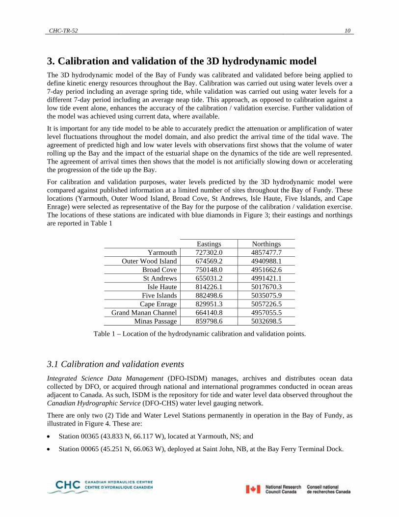
3. Calibration and validation of the 3D hydrodynamic model The 3D hydrodynamic model of the Bay of Fundy was calibrated and validated before being applied to define kinetic energy resources throughout the Bay. Calibration was carried out using water levels over a 7-day period including an average spring tide, while validation was carried out using water levels for a different 7-day period including an average neap tide. This approach, as opposed to calibration against a low tide event alone, enhances the accuracy of the calibration / validation exercise. Further validation of the model was achieved using current data, where available.
It is important for any tide model to be able to accurately predict the attenuation or amplification of water level fluctuations throughout the model domain, and also predict the arrival time of the tidal wave. The agreement of predicted high and low water levels with observations first shows that the volume of water rolling up the Bay and the impact of the estuarial shape on the dynamics of the tide are well represented. The agreement of arrival times then shows that the model is not artificially slowing down or accelerating the progression of the tide up the Bay.
For calibration and validation purposes, water levels predicted by the 3D hydrodynamic model were compared against published information at a limited number of sites throughout the Bay of Fundy. These locations (Yarmouth, Outer Wood Island, Broad Cove, St Andrews, Isle Haute, Five Islands, and Cape Enrage) were selected as representative of the Bay for the purpose of the calibration / validation exercise. The locations of these stations are indicated with blue diamonds in Figure 3; their eastings and northings are reported in Table 1
Eastings Northings
Yarmouth 727302.0 4857477.7 Outer Wood Island 674569.2 4940988.1
Broad Cove 750148.0 4951662.6 St Andrews 655031.2 4991421.1
Isle Haute 814226.1 5017670.3 Five Islands 882498.6 5035075.9
Cape Enrage 829951.3 5057226.5 Grand Manan Channel 664140.8 4957055.5
Minas Passage 859798.6 5032698.5
Table 1 – Location of the hydrodynamic calibration and validation points.
3.1 Calibration and validation events Integrated Science Data Management (DFO-ISDM) manages, archives and distributes ocean data collected by DFO, or acquired through national and international programmes conducted in ocean areas adjacent to Canada. As such, ISDM is the repository for tide and water level data observed throughout the Canadian Hydrographic Service (DFO-CHS) water level gauging network.
There are only two (2) Tide and Water Level Stations permanently in operation in the Bay of Fundy, as illustrated in Figure 4. These are:
• Station 00365 (43.833 N, 66.117 W), located at Yarmouth, NS; and
• Station 00065 (45.251 N, 66.063 W), deployed at Saint John, NB, at the Bay Ferry Terminal Dock.

CHC-TR-52 11
Figure 4 – Map of the DFO gauging network along the East Coast (Reference 12).
Station 00365 is closest to the offshore boundary of the 3D hydrodynamic model. Data from Station 00365 for the year 2007 was retrieved from DFO-ISDM’s web site (Reference 12) for analysis. Observed water levels were available at hourly intervals between January 1st, 2007 and December 23rd, 2007, with only a few minor interruptions in the records. Common parameters were derived from the time series and compared to those reported for Yarmouth in the DFO-CHS tide tables (Reference 13). The results of the comparison are summarized in Table 2. In light of this comparison, 2007 is believed to be a “normal” year and water level data from 2007 can therefore be used with reasonable confidence to derive average conditions.
Reported in
DFO-CHS tide tables
Derived from 2007 observed
water levels mean water level 2.6 m CD 2.6 m CD
higher high water 5.2 m CD 5.2 m CD Large tide lower low water 0.0 m CD -0.1 m CD Mean tide higher high water 4.5 m CD 4.6 m CD
Table 2 – Tidal heights and mean water level at Yarmouth.
Spring tides are the semidiurnal tides of greatest range in a semi-lunation of 15 days, while neap tides are the semidiurnal tides of smallest range within that period. The water level data observed at Yarmouth were closely examined and the maximum and minimum high waters were extracted for each 15-day period of the year (25 cycles per year), leading to a set of 25 high water springs and 25 high water neaps. Average spring and average neap conditions were determined from analysis of the 25 15-day cycles recorded during 2007. The resulting average spring and average neap tides at Yarmouth are presented in Table 3.

CHC-TR-52 12
Mean High Water Springs 4.8 m CD 2.2 m GD Mean High Water Neaps 3.7 m CD 1.1 m GD
Table 3 – Average spring and average neap conditions at Yarmouth.
The numerical model developed by the Department of Fisheries and Oceans to calculate tidal harmonic constituents in the Bay of Fundy (Scotian Shelf model – Reference 11) was used in this study to generate spatially distributed and time-varying water levels at the boundary of the 3D hydrodynamic model.
The water level time series predicted at Yarmouth from the harmonics was closely analysed. Two 7-day periods were identified which matched the average spring and average neap conditions respectively. These two periods were selected for simulation in the 3D hydrodynamic model.
3.2 Calibration / validation of the 3D hydrodynamic model To calibrate the 3D hydrodynamic model, the friction factor associated with bottom roughness was adjusted by varying the Strickler roughness coefficient throughout the model domain to improve the agreement between the predicted and measured water levels throughout the Bay of Fundy.
In the absence of measured water levels throughout the Bay, the 3D hydrodynamic model was calibrated and validated against published information from the DFO-CHS tide tables at a number of reference and secondary Ports (shown as blue diamonds in Figure 3). Although the use of predicted values is generally not preferred to calibrate a model, it was necessary in this study since no other reliable data were available.
The water levels (highs and lows) predicted from the Canadian Hydrographic Service tide tables were therefore extracted for a period equivalent to the average spring and average neap conditions simulated in the 3D hydrodynamic model.
It is important to stress at this stage that, in an effort to define the best possible boundary conditions for the model, the water levels simulated at the boundary were not derived from the tide tables, but rather were developed from the harmonic constituents predicted by DFO’s Scotian Shelf model (Reference 11). In essence there is no timeline associated with the water level time series generated from these harmonic constituents.
To allow direct comparison of the model results with published information, the water levels predicted from the 2007 tide tables (Reference 13) were therefore scanned to find the best possible match to the 7-day signals synthesized at Yarmouth. The following two time periods were identified for the average spring and average neap tides:
• Calibration period: August 28, 2007 8:30 PM to September 4, 2007 8:30 PM (7-day period including the average spring tide); and
• Validation period: September 14, 2007 10:15 PM to September 21, 2007 10:15 PM (7-day period including the average neap tide).
It should be noted that while these time intervals were selected to minimize the differences between the tide tables and the water level signals synthesized from the Scotian Shelf model constituents, the agreement was imperfect and some discrepancies remained.
Figure 5 to Figure 11 show the water levels predicted by the 3D hydrodynamic model (line) at the various calibration sites (Yarmouth, Outer Wood Island, Broad Cove, St Andrews, Isle Haute, Five Islands, and Cape Enrage) for the 7-day calibration period, compared to highs and lows published in the DFO-CHS tide tables for the same period (diamonds). The 3D hydrodynamic model clearly provides a reasonable prediction of both the phase and amplitude of the spring tide at each station. The quality of the calibration

CHC-TR-52 13
was assessed by calculating the average difference in high and low water elevation between the model predictions and the published values over the calibration period. The results of this assessment are summarized in Table 4 in terms of absolute difference (in meters) and also as a percentage of the tidal range. The average difference in the time of arrival of high water was also calculated and is expressed in Table 4 as a percentage of the 745 minute tidal cycle. The high and low water levels at five of the seven Stations are predicted to within 3%. The maximum difference at the other two Stations is less than 7% of the tidal range. The arrival time of high water is predicted to within 14 minutes at six of the seven stations.
-3
-2
-1
0
1
2
3
28/08/2007 20:30 29/08/2007 20:30 30/08/2007 20:30 31/08/2007 20:30 01/09/2007 20:30 02/09/2007 20:30 03/09/2007 20:30 04/09/2007 20:30
wat
er le
vel (
mG
D)
Yarmouth - Predicted resultYarmouth - Available data sample
Figure 5 – 3D calibration: water level at Yarmouth, August 28 to September 4, 2007.
-4
-3
-2
-1
0
1
2
3
4
28/08/2007 20:30 29/08/2007 20:30 30/08/2007 20:30 31/08/2007 20:30 01/09/2007 20:30 02/09/2007 20:30 03/09/2007 20:30 04/09/2007 20:30
wat
er le
vel (
mG
D)
Outer Wood Island - Predicted resultOuter Wood Island - Available data sample
Figure 6 – 3D calibration: water level at Outer Wood Island, August 28 to September 4, 2007.

CHC-TR-52 14
-5
-4
-3
-2
-1
0
1
2
3
4
5
28/08/2007 20:30 29/08/2007 20:30 30/08/2007 20:30 31/08/2007 20:30 01/09/2007 20:30 02/09/2007 20:30 03/09/2007 20:30 04/09/2007 20:30
wat
er le
vel (
mG
D)
Broad Cove - Predicted resultBroad Cove - Available data sample
Figure 7 – 3D calibration: water level at Broad Cove, August 28 to September 4, 2007.
-5
-4
-3
-2
-1
0
1
2
3
4
5
28/08/2007 20:30 29/08/2007 20:30 30/08/2007 20:30 31/08/2007 20:30 01/09/2007 20:30 02/09/2007 20:30 03/09/2007 20:30 04/09/2007 20:30
wat
er le
vel (
mG
D)
St Andrews - Predicted resultSt Andrews - Available data sample
Figure 8 – 3D calibration: water level at St Andrews, August 28 to September 4, 2007.
-6
-4
-2
0
2
4
6
28/08/2007 20:30 29/08/2007 20:30 30/08/2007 20:30 31/08/2007 20:30 01/09/2007 20:30 02/09/2007 20:30 03/09/2007 20:30 04/09/2007 20:30
wat
er le
vel (
mG
D)
Isle Haute - Predicted resultIsle Haute - Available data sample
Figure 9 – 3D calibration: water level at Isle Haute, August 28 to September 4, 2007.

CHC-TR-52 15
-8
-6
-4
-2
0
2
4
6
8
28/08/2007 20:30 29/08/2007 20:30 30/08/2007 20:30 31/08/2007 20:30 01/09/2007 20:30 02/09/2007 20:30 03/09/2007 20:30 04/09/2007 20:30
wat
er le
vel (
mG
D)
Five Islands - Predicted resultFive Islands - Available data sample
Figure 10 – 3D calibration: water level at Five Islands, August 28 to September 4, 2007.
-8
-6
-4
-2
0
2
4
6
8
28/08/2007 20:30 29/08/2007 20:30 30/08/2007 20:30 31/08/2007 20:30 01/09/2007 20:30 02/09/2007 20:30 03/09/2007 20:30 04/09/2007 20:30
wat
er le
vel (
mG
D)
Cape Enrage - Predicted resultCape Enrage - Available data sample
Figure 11 – 3D calibration: water level at Cape Enrage, August 28 to September 4, 2007.
Location Low water level High water level Time of arrival
of high water Yarmouth --
(-0.01 m) within 2% (0.08 m)
on time (-1 min)
Outer Wood Island within 3% (-0.16 m)
within 2% (0.10 m)
within 1% (-5 min)
Broad Cove within 7% (0.53 m)
within 5% (0.36 m)
on time (-3 min)
St Andrews within 1% (0.10 m)
within 1% (-0.04 m)
within 3% (-21 min)
Isle Haute within 7% (-0.59 m)
within 6% (0.49 m)
within 2% (14 min)
Five Islands -- (-0.05 m)
within 1% (-0.11 m)
on time (-1 min)
Cape Enrage within 2% (-0.22 m)
within 3% (0.34 m)
within 1% (6 min)
Table 4 – 3D hydrodynamic model calibration results, average spring tide.

CHC-TR-52 16
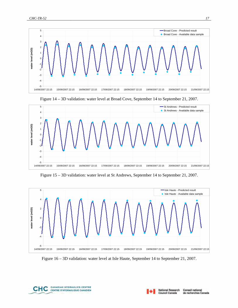
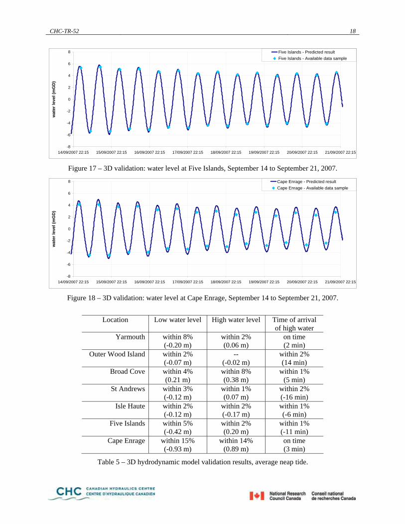
The same exercise was repeated for the 7-day validation period corresponding to an average neap tide. The results are displayed in Figure 12 to Figure 18 and summarized in Table 5. The arrival time of high water at all seven stations is predicted with a precision of 16 minutes or better. The high and low water levels at six of the seven Stations are predicted to within 8% or better. The tide range at Cape Enrage was slightly over-predicted during the average neap tide, but well-predicted during the average spring tide.
It is important to recognize that these small differences could be due to deficiencies in the new numerical model, or could be due to the fact the that the hydrodynamic model was forced using boundary conditions derived from tidal constituents (obtained from results of DFO’s Scotian Shelf model), and not from the tide tables. Overall, these results indicate that the 3D hydrodynamic model provides a reasonable prediction of water level fluctuations throughout the Bay of Fundy for both spring and neap tides.
-3
-2
-1
0
1
2
3
14/09/2007 22:15 15/09/2007 22:15 16/09/2007 22:15 17/09/2007 22:15 18/09/2007 22:15 19/09/2007 22:15 20/09/2007 22:15 21/09/2007 22:15
wat
er le
vel (
mG
D)
Yarmouth - Predicted resultYarmouth - Available data sample
Figure 12 – 3D validation: water level at Yarmouth, September 14 to September 21, 2007.
-4
-3
-2
-1
0
1
2
3
4
14/09/2007 22:15 15/09/2007 22:15 16/09/2007 22:15 17/09/2007 22:15 18/09/2007 22:15 19/09/2007 22:15 20/09/2007 22:15 21/09/2007 22:15
wat
er le
vel (
mG
D)
Outer Wood Island - Predicted resultOuter Wood Island - Available data sample
Figure 13 – 3D validation: water level at Outer Wood Island, September 14 to September 21, 2007.
CHC-TR-52 17
-5
-4
-3
-2
-1
0
1
2
3
4
5
14/09/2007 22:15 15/09/2007 22:15 16/09/2007 22:15 17/09/2007 22:15 18/09/2007 22:15 19/09/2007 22:15 20/09/2007 22:15 21/09/2007 22:15
wat
er le
vel (
mG
D)
Broad Cove - Predicted resultBroad Cove - Available data sample
Figure 14 – 3D validation: water level at Broad Cove, September 14 to September 21, 2007.
-5
-4
-3
-2
-1
0
1
2
3
4
5
14/09/2007 22:15 15/09/2007 22:15 16/09/2007 22:15 17/09/2007 22:15 18/09/2007 22:15 19/09/2007 22:15 20/09/2007 22:15 21/09/2007 22:15
wat
er le
vel (
mG
D)
St Andrews - Predicted resultSt Andrews - Available data sample
Figure 15 – 3D validation: water level at St Andrews, September 14 to September 21, 2007.
-6
-4
-2
0
2
4
6
14/09/2007 22:15 15/09/2007 22:15 16/09/2007 22:15 17/09/2007 22:15 18/09/2007 22:15 19/09/2007 22:15 20/09/2007 22:15 21/09/2007 22:15
wat
er le
vel (
mG
D)
Isle Haute - Predicted resultIsle Haute - Available data sample
Figure 16 – 3D validation: water level at Isle Haute, September 14 to September 21, 2007.
CHC-TR-52 18
-8
-6
-4
-2
0
2
4
6
8
14/09/2007 22:15 15/09/2007 22:15 16/09/2007 22:15 17/09/2007 22:15 18/09/2007 22:15 19/09/2007 22:15 20/09/2007 22:15 21/09/2007 22:15
wat
er le
vel (
mG
D)
Five Islands - Predicted resultFive Islands - Available data sample
Figure 17 – 3D validation: water level at Five Islands, September 14 to September 21, 2007.
-8
-6
-4
-2
0
2
4
6
8
14/09/2007 22:15 15/09/2007 22:15 16/09/2007 22:15 17/09/2007 22:15 18/09/2007 22:15 19/09/2007 22:15 20/09/2007 22:15 21/09/2007 22:15
wat
er le
vel (
mG
D)
Cape Enrage - Predicted resultCape Enrage - Available data sample
Figure 18 – 3D validation: water level at Cape Enrage, September 14 to September 21, 2007.
Location Low water level High water level Time of arrival
of high water Yarmouth within 8%
(-0.20 m) within 2% (0.06 m)
on time (2 min)
Outer Wood Island within 2% (-0.07 m)
-- (-0.02 m)
within 2% (14 min)
Broad Cove within 4% (0.21 m)
within 8% (0.38 m)
within 1% (5 min)
St Andrews within 3% (-0.12 m)
within 1% (0.07 m)
within 2% (-16 min)
Isle Haute within 2% (-0.12 m)
within 2% (-0.17 m)
within 1% (-6 min)
Five Islands within 5% (-0.42 m)
within 2% (0.20 m)
within 1% (-11 min)
Cape Enrage within 15% (-0.93 m)
within 14% (0.89 m)
on time (3 min)
Table 5 – 3D hydrodynamic model validation results, average neap tide.

CHC-TR-52 19
3.3 Additional verification of the 3D hydrodynamic model Additional verification of the model was achieved through a comparison of predicted current velocities (amplitude and direction) in Grand Manan Channel against velocities predicted current tables published by DFO-CHS (Reference 13). The location of this point is shown in Figure 3 as a red circle next to Outer Wood Island.
In Grand Manan Channel, the flood current sets in a general north-easterly direction (predicted by DFO-CHS at 32°N) and attains a speed of about 2.0 m/s at strength for an average spring tide, and 1.0 m/s for an average neap tide. The ebb sets in a south-westerly direction (predicted by DFO-CHS at 212°N) with a speed of about 1.8 m/s at strength for an average spring tide, and 0.75 m/s for an average neap tide. In the absence of explicit information, it was assumed that the current tables refer to surface currents, which are relevant for navigation purposes. They were compared to the currents predicted from the 3D hydrodynamic model on the topmost layer.
The average difference in maximum (flooding and ebbing) current speeds between the model predictions and the published values were calculated and expressed as a percentage of the flow speed range for an average spring tide and an average neap tide. The average difference in current direction was also calculated. Finally the average time when maximum (flood) currents occur was calculated and expressed as a percentage of a tidal cycle of 745 minutes. The results of this analysis are presented in Table 6 and in Figure 19 to Figure 22. In these figures the 3D hydrodynamic model predictions are shown in dark blue, while the values predicted and published in the DFO-CHS current tables are shown in light blue.
The direction of the surface currents predicted by the new 3D hydrodynamic model is in very good agreement with the directions published in the current tables. However, the peak current speeds predicted by the new model are slightly smaller than the published values. It is important to recognize that these differences could be due to deficiencies in the new numerical model or deficiencies in the published values, or a combination of the two.
Location Flooding Ebbing
Max. speed Direction Max. speed Direction
Time of slack currents
Grand Manan Channel (average spring tide)
within 9% (-0.3 m/s)
within 7% (0.2 m/s)
on time (2 min)
Grand Manan Channel (average neap tide)
within 4% (-0.1 m/s)
-- (-1 °N) within 2%
(-0.1 m/s)
within 2% (7 °N)
within 5% (39 min)
Table 6 – Comparison of surface current predictions in Grand Manan Channel.
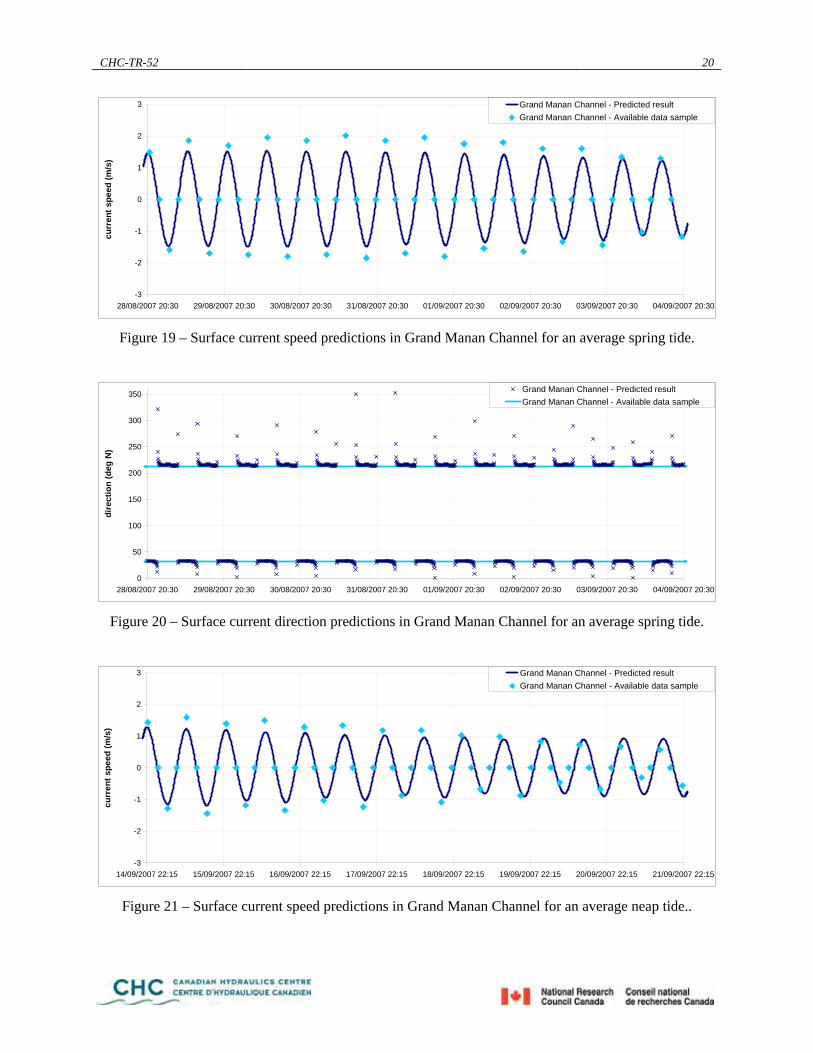
CHC-TR-52 20
-3
-2
-1
0
1
2
3
28/08/2007 20:30 29/08/2007 20:30 30/08/2007 20:30 31/08/2007 20:30 01/09/2007 20:30 02/09/2007 20:30 03/09/2007 20:30 04/09/2007 20:30
curr
ent s
peed
(m/s
)Grand Manan Channel - Predicted resultGrand Manan Channel - Available data sample
Figure 19 – Surface current speed predictions in Grand Manan Channel for an average spring tide.
0
50
100
150
200
250
300
350
28/08/2007 20:30 29/08/2007 20:30 30/08/2007 20:30 31/08/2007 20:30 01/09/2007 20:30 02/09/2007 20:30 03/09/2007 20:30 04/09/2007 20:30
dire
ctio
n (d
eg N
)
Grand Manan Channel - Predicted resultGrand Manan Channel - Available data sample
Figure 20 – Surface current direction predictions in Grand Manan Channel for an average spring tide.
-3
-2
-1
0
1
2
3
14/09/2007 22:15 15/09/2007 22:15 16/09/2007 22:15 17/09/2007 22:15 18/09/2007 22:15 19/09/2007 22:15 20/09/2007 22:15 21/09/2007 22:15
curr
ent s
peed
(m/s
)
Grand Manan Channel - Predicted resultGrand Manan Channel - Available data sample
Figure 21 – Surface current speed predictions in Grand Manan Channel for an average neap tide..
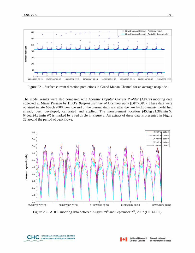
CHC-TR-52 21
0
50
100
150
200
250
300
350
14/09/2007 22:15 15/09/2007 22:15 16/09/2007 22:15 17/09/2007 22:15 18/09/2007 22:15 19/09/2007 22:15 20/09/2007 22:15 21/09/2007 22:15
dire
ctio
n (d
eg N
)
Grand Manan Channel - Predicted resultGrand Manan Channel - Available data sample
Figure 22 – Surface current direction predictions in Grand Manan Channel for an average neap tide.
The model results were also compared with Acoustic Doppler Current Profiler (ADCP) mooring data collected in Minas Passage by DFO’s Bedford Institute of Oceanography (DFO-BIO). These data were obtained in late March 2008, near the end of the present study and after the new hydrodynamic model had already been developed, calibrated and applied. The measurement location (45deg 21.389min N; 64deg 24.23min W) is marked by a red circle in Figure 3. An extract of these data is presented in Figure 23 around the period of peak flows.
0.0
0.5
1.0
1.5
2.0
2.5
3.0
3.5
4.0
4.5
5.0
29/08/2007 20:30 30/08/2007 20:30 31/08/2007 20:30 01/09/2007 20:30 02/09/2007 20:30
curr
ent s
peed
(m/s
)
48 m from bottom
40 m from bottom
26 m from bottom
12 m from bottom
8 m from bottom
Figure 23 – ADCP mooring data between August 29th and September 2nd, 2007 (DFO-BIO).

CHC-TR-52 22
The mooring was deployed on August 17th, 2007 and recovered on September 14th, 2007. There is only a minor interruption in the records (1.5 hrs on August 28th), during which time the mooring was recovered briefly to extract the initial data and check the mooring. The ADCP current data were measured every 2 m throughout the water column (between 8 m and 52 m from the bottom). The water depth at this location is said to vary between 47 m and 59 m depending on the stage of the tide. Typically, surface flows are not measured by an ADCP.
Figure 24, Figure 25 and Figure 26 present time histories of orthogonal velocity components at three different elevations predicted by the new 3D hydrodynamic model (triangles) at the ADCP mooring, compared to the ADCP data (lines) for the same period around peak flows.
The observed agreement between the 3D hydrodynamic model predictions and the field measurements is very good for the principal east-west component. The agreement is slightly less satisfactory but still reasonable for the north-south velocity component. The observed attenuation with depth is also well predicted by the new hydrodynamic model. This comparison enhances the confidence in the numerical model predictions.
-5.0
-4.0
-3.0
-2.0
-1.0
0.0
1.0
2.0
3.0
4.0
5.0
29/08/2007 20:30 30/08/2007 20:30 31/08/2007 20:30 01/09/2007 20:30 02/09/2007 20:30
velo
city
(m/s
)
E-W velocity - Predicted result E-W velocity - Available data sampleN-S velocity - Predicted result N-S velocity - Available data sample
Figure 24 – Comparison of predicted and measured velocities in Minas Passage, 40 m from bottom.

CHC-TR-52 23
-5.0
-4.0
-3.0
-2.0
-1.0
0.0
1.0
2.0
3.0
4.0
5.0
29/08/2007 20:30 30/08/2007 20:30 31/08/2007 20:30 01/09/2007 20:30 02/09/2007 20:30
velo
city
(m/s
)E-W velocity - Predicted result E-W velocity - Available data sampleN-S velocity - Predicted result N-S velocity - Available data sample
Figure 25 – Comparison of predicted and measured velocities in Minas Passage, 26 m from bottom.
-5.0
-4.0
-3.0
-2.0
-1.0
0.0
1.0
2.0
3.0
4.0
5.0
29/08/2007 20:30 30/08/2007 20:30 31/08/2007 20:30 01/09/2007 20:30 02/09/2007 20:30
velo
city
(m/s
)
E-W velocity - Predicted result E-W velocity - Available data sampleN-S velocity - Predicted result N-S velocity - Available data sample
Figure 26 – Comparison of predicted and measured velocities in Minas Passage, 12 m from bottom.

CHC-TR-52 24
The ability of the new 3D hydrodynamic model to simulate water level fluctuations and currents within the Bay of Fundy has been demonstrated and compared with several other types of data, both measured and predicted. Overall, these results indicate that the new 3D hydrodynamic model is able to provide good predictions of water level fluctuations and currents throughout the Bay of Fundy for both spring and neap tides. The model can be applied to investigate tidal currents in areas previously identified as having substantial kinetic energy resources, namely: Minas Passage, NS; Petit Passage, Grand Passage, NS; Digby Gut, NS; Western Passage, NB; Head Harbour Passage, NB; and Letete Passage, NB.
CHC-TR-52 25
4. Simulation Results and Tidal Energy Resource Assessment
4.1 Previous Assessments of Kinetic Energy Resources It is worth recalling that tidal currents vary rapidly with space and time. At most sites, the flow velocity approaches zero from two to four times per day, and reaches its peak annual value for only a few hours per year. The velocity fluctuation during each half cycle is roughly sinusoidal, but the peak speed varies from cycle to cycle as a consequence of the lunar and solar gravitational forcing. At most sites, the direction of flow also reverses between two and four times per day.
Tidal current resources are best characterized by the mean power, which represents an integration or averaging of these temporal fluctuations over time. The annual mean power is the average value of the instantaneous power throughout the year. Similarly, the mean power density is the average value of the instantaneous power density over time. The mean power density characterizes the average intensity of the flow at the site, while the mean power indicates the scale of the energy resource. Energy extraction will not be feasible if the flows are too weak for efficient operation of an energy conversion device. Safe installation, operation and maintenance could also be difficult if the flows are excessively strong.
In 2006 the Canadian Hydraulics Centre of the National Research Council (NRC-CHC) led a team that studied wave energy and tidal kinetic energy resources across Canada, including in the Bay of Fundy. The study was funded by Natural Resources Canada. While no new numerical modelling was undertaken for this study, results from fourteen existing computer models of tidal flows were assembled, reviewed and used in the assessment. Potential tidal sites were identified and assessed by employing the following 3-step process:
• identifying passages and reaches with strong tidal currents;
• determining and/or estimating basic parameters for each site, including the passage width, average depth, and the maximum ebb and flood velocities during large tides; and
• estimating the annual mean power density and annual mean power from these basic parameters.
A summary of the results obtained for sites on the Bay of Fundy is presented in Table 7. It is important to note that these estimates reflect the total kinetic energy available in the tidal flows, and that the extractable resource will be significantly smaller.

CHC-TR-52 26
Site Name
Latitude
Longitude
Maxim
um C
urrent S
peed Flood
Maxim
um C
urrent S
peed Ebb
Mean M
aximum
D
epth Average
Current S
peed
Mean P
ower
Density
Width of P
assage
Average Depth of
Passage
Flow C
ross-sectional A
rea
Mean P
otential P
ower
deg deg knot knot m/s kW/m2 m m m2 MW Miramichi Bay Islands 47.15 -65.04 3.5 3.5 1.53 0.42 1,920 5 10,944 5 Clarks Ground 44.59 -66.64 6 6 2.63 2.11 4,092 22 102,300 216 Devils Half Acre 44.54 -66.69 6 6 2.63 2.11 2,133 18 44,793 95 Old Sow 44.92 -66.99 6 6 2.63 2.11 625 60 39,375 83 Head Harbour Passage 1 44.95 -66.93 5 5 2.19 1.22 890 65 60,520 74 Gran Manan Channel 44.78 -66.86 2.5 2 0.98 0.11 5,446 80 452,018 50 Quoddy River 44.96 -66.95 4.5 4 1.86 0.75 1,350 28 41,850 31 Reversing Falls 45.26 -66.09 12 12 5.25 16.88 90 15 1,746 29 Cumberland Basin 45.74 -64.47 4 5 1.97 0.89 2,125 6 26,988 24 Letete Passage 45.05 -66.92 5 5 2.19 1.22 508 25 14,224 17 Shepody Bay 45.87 -64.57 3 4 1.53 0.42 1,400 3 12,740 5 Lubec Narrows 44.86 -66.98 6 8 3.06 3.35 180 3 1,080 4 Little Letete Passage 45.03 -66.93 5 5 2.19 1.22 150 6 1,350 2 Devils Head/St Stephen 45.16 -67.18 3 4 1.53 0.42 440 3 2,640 1 Minas Passage 45.35 -64.40 7.5 7.5 3.28 6.04 4,376 56 274,113 1,903Northwest Ledge 44.30 -66.42 4 4 1.75 0.63 5,334 18 117,348 73 The Hospital 43.44 -66.00 4 4 1.75 0.63 3,600 18 79,200 50 Petit Passage 44.39 -66.21 7 7 3.06 3.35 335 18 7,035 24 Digby Gut 44.68 -65.76 5 5 2.19 1.22 573 25 16,904 21 Grand Passage 44.28 -66.34 6 6 2.63 2.11 380 16 7,220 15 Trinity Ledge 44.00 -66.29 2.5 2.5 1.09 0.15 2,520 14 42,840 7 Ellewoods Channel 43.66 -66.05 4 4 1.75 0.63 350 4 2,275 1
Table 7 – Summary of tidal kinetic energy resources in the Bay of Fundy (Reference 11).
In 2006 the Electric Power Research Institute studied areas in Nova Scotia, New Brunswick and Maine (United States) with potential to generate renewable energy through the use of tidal in-stream technologies (Reference 6 to Reference 8). Fifteen potential locations were identified in the Bay of Fundy. Their work was funded by the Nova Scotia Department of Energy, Nova Scotia Power Inc., New Brunswick Department of Energy, New Brunswick Power and the Maine Technology Initiative.
EPRI made use of available information to derive their estimates. They considered published sources (nautical charts, current tables, sailing directions) to determine the current speed for each area. No new modelling studies or field measurements were undertaken. With the assumptions that the reported values were maximum current speeds at the surface, that velocity time series profiles from peak to slack currents could be approximated by sinusoidal curves, and that the vertical velocity profile followed a 1/10 power curve, they were able to convert the published current speeds to depth-averaged peak and mean (representative of a year) values. Estimates of depth-averaged mean power density for peak flows and for the entire year were obtained from the depth-averaged velocities. The conclusions of the EPRI studies are summarized in Table 8.
CHC-TR-52 27
Depth-averaged mean power density Location
peak flows only the entire year Mean extractable
power 1
NEW BRUNSWICK Lubec Narrows 16 kW/m2 5.5 kW/m2 1.2 megawatts (MW)
Western Passage 5.1 kW/m2 2.2 kW/m2 10.8 MW Head Harbour Passage 4.5 kW/m2 1.9 kW/m2 14.0 MW
Letete Passage 8.7 kW/m2 3.7 kW/m2 4.2 MW Saint John River to be determined to be determined to be determined
Cape Enrage 1.0 kW/m2 0.42 kW/m2 30.0 MW Shepody Bay 1.9 kW/m2 0.81 kW/m2 13.0 MW
Cumberland Basin 6.4 kW/m2 2.7 kW/m2 16.7 MW
NOVA SCOTIA Cumberland Basin 4.9 kW/m2 2.1 kW/m2 6.5 MW
Minas Channel 4.9 kW/m2 2.1 kW/m2 131 MW Minas Passage 11.5 kW/m2 4.9 kW/m2 166 MW Cobequid Bay 3.0 kW/m2 1.0 kW/m2 6.3 MW
Digby Gut 4.3 kW/m2 1.8 kW/m2 4.9 MW Petit Passage 18 kW/m2 7.7 kW/m2 9.2 MW
Grand Passage 11.5 kW/m2 4.9 kW/m2 6.6 MW
Table 8 – Summary of tidal in-stream energy resources in the Bay of Fundy (Reference 7 and Reference 8).
4.2 Simulation Results for Selected Areas in Nova Scotia To characterize the energy resources in the Bay of Fundy, the new 3D hydrodynamic model was applied to simulate a 15-day period including an average spring and an average neap tide. Conditions during this 15-day period can be considered indicative of conditions over long durations containing many more tide cycles. In particular, the mean or average conditions during the 15-day period should be very similar to the mean conditions for longer periods. However, the maximum conditions predicted by the model over the 15-day period will under-estimate the extreme conditions that will occur in nature over longer durations.
In what follows, results from three-dimensional hydrodynamic model simulations are presented for a limited number of areas, shown in Figure 27. These sites are amongst those previously identified by NRC-CHC (Reference 11) and EPRI (Reference 7, Reference 8). The sites in Nova Scotia are: Minas Passage; Petit Passage; Grand Passage; and Digby Gut. The sites in New Brunswick are: Western Passage; Head Harbour Passage and Letete Passage. Readers are reminded that this 3D hydrodynamic model was developed to provide detailed predictions of the flows in these specific areas. Less reliable predictions should be expected in the Saint John River and in the extreme upper parts of the Bay.
In this report, simulation results are presented in terms of current speeds U (m/s) and kinetic power density 35.0 UP ρ= (kW/m2), where ρ is the water density in kg/m3. P denotes the rate of energy per square meter cross-section. For example, consider a flow of water with velocity 1 m/s flowing through a
1 based on the assumption that 15 percent of the tidal in-stream energy could be extracted without causing significant environmental impacts. This assumption has not been verified.
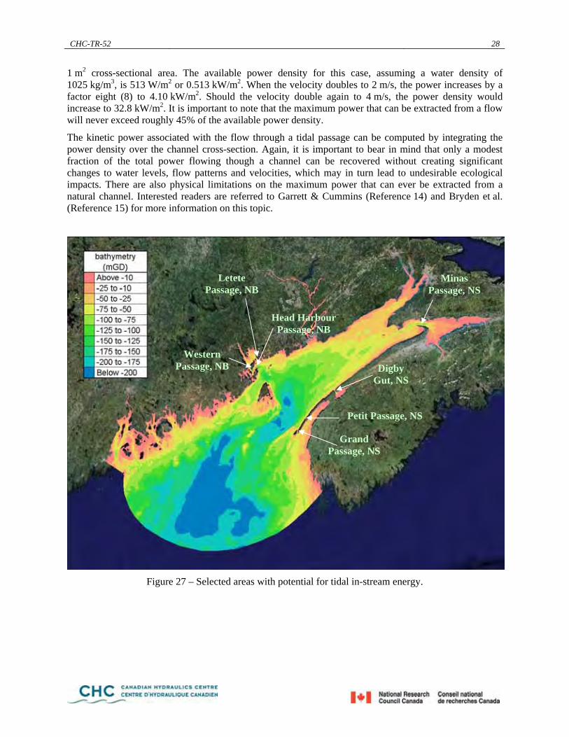
CHC-TR-52 28
1 m2 cross-sectional area. The available power density for this case, assuming a water density of 1025 kg/m3, is 513 W/m2 or 0.513 kW/m2. When the velocity doubles to 2 m/s, the power increases by a factor eight (8) to 4.10 kW/m2. Should the velocity double again to 4 m/s, the power density would increase to 32.8 kW/m2. It is important to note that the maximum power that can be extracted from a flow will never exceed roughly 45% of the available power density.
The kinetic power associated with the flow through a tidal passage can be computed by integrating the power density over the channel cross-section. Again, it is important to bear in mind that only a modest fraction of the total power flowing though a channel can be recovered without creating significant changes to water levels, flow patterns and velocities, which may in turn lead to undesirable ecological impacts. There are also physical limitations on the maximum power that can ever be extracted from a natural channel. Interested readers are referred to Garrett & Cummins (Reference 14) and Bryden et al. (Reference 15) for more information on this topic.
Figure 27 – Selected areas with potential for tidal in-stream energy.
Grand Passage, NS
Petit Passage, NS
Digby Gut, NS
Minas Passage, NS
Letete Passage, NB
Western Passage, NB
Head Harbour Passage, NB

CHC-TR-52 29
In this report the 3D hydrodynamic model results for each area of interest are displayed in several different ways, described below.
• Streamlines, which are lines tangent at any point to the currents and give a good indication of the predicted flow pathways. Streamlines are presented at four (4) points in the tide cycle to illustrate the different current patterns depending on the stage of the tide: near high water (slack currents), mean water (peak ebb currents), low water (slack currents), and mean water (peak flood currents). In these figures the thick red lines represent streamlines, the arrows represent depth-averaged velocities (magnitude shown by the colour scale, and direction), and the underlying colour contour map represents the water depth (with respect to mean water level).
• Vertical cross-sections, or slices, of predicted three-dimensional current speed and kinetic power density showing the variability with location and elevation. These are presented as filled colour contour maps for peak flood and peak ebb flows (same times as the streamlines). It should be emphasized that these plots show instantaneous conditions at specific (favourable) times and should not be regarded as representative of conditions throughout the tidal cycle. The locations of the profiles were selected to include high-energy points. These locations are shown as thick red lines in Figure 28, Figure 81, Figure 59 and Figure 103 for each area of interest.
• Time histories of predicted depth-averaged current speed and depth-averaged kinetic power density at one high-energy point for the 7-day periods corresponding to average spring and average neap conditions. The location of this point is displayed as a yellow star in Figure 28, Figure 81, Figure 59 and Figure 103 for each area of interest.
• Cumulative probability distributions at one high-energy point (the same as for previous analysis) of predicted depth-averaged current speed and depth-averaged kinetic power density for the 7-day periods corresponding to average spring and neap conditions.
• Velocity roses of predicted depth-averaged current speed at the same high-energy point and 7-day periods. A velocity rose is a visual representation of the frequency of occurrence of certain conditions, lumped into directional sectors and current speed bins. In this analysis we used 30° directional bins and speed intervals between 0.25 m/s and 1 m/s. Each ring on the rose represents a frequency of occurrence of 12.5%. The width of the color bars represents the frequency of occurrence of a current from a given direction and within a certain range.
• Colour contour maps showing the spatial variations of predicted depth-averaged mean current speed and mean kinetic power density. These maps were produced by calculating the temporal average of the depth-averaged current speed / power density at each model grid point over the 7-day periods corresponding to average spring or neap conditions.
• Colour contour maps showing the spatial variations of predicted depth-averaged maximum current speed and maximum power density. These maps were produced by computing the maximum value of the depth-averaged current speed / power density at each model grid point over the 7-day periods including average spring or neap conditions.
Simulation results from the new 3D hydrodynamic model for four parts of the Bay of Fundy in Nova Scotia have been studied in detail to investigate their potential for tidal in-stream energy: Petit Passage and Grand Passage at the entrance to the Bay of Fundy, Digby Gut at the confluence of the Bay with the Annapolis River and Minas Passage, near the head of the Bay of Fundy. Detailed simulation results for these areas are presented in Sections 4.2.1, 4.2.2, and 4.2.3 respectively.
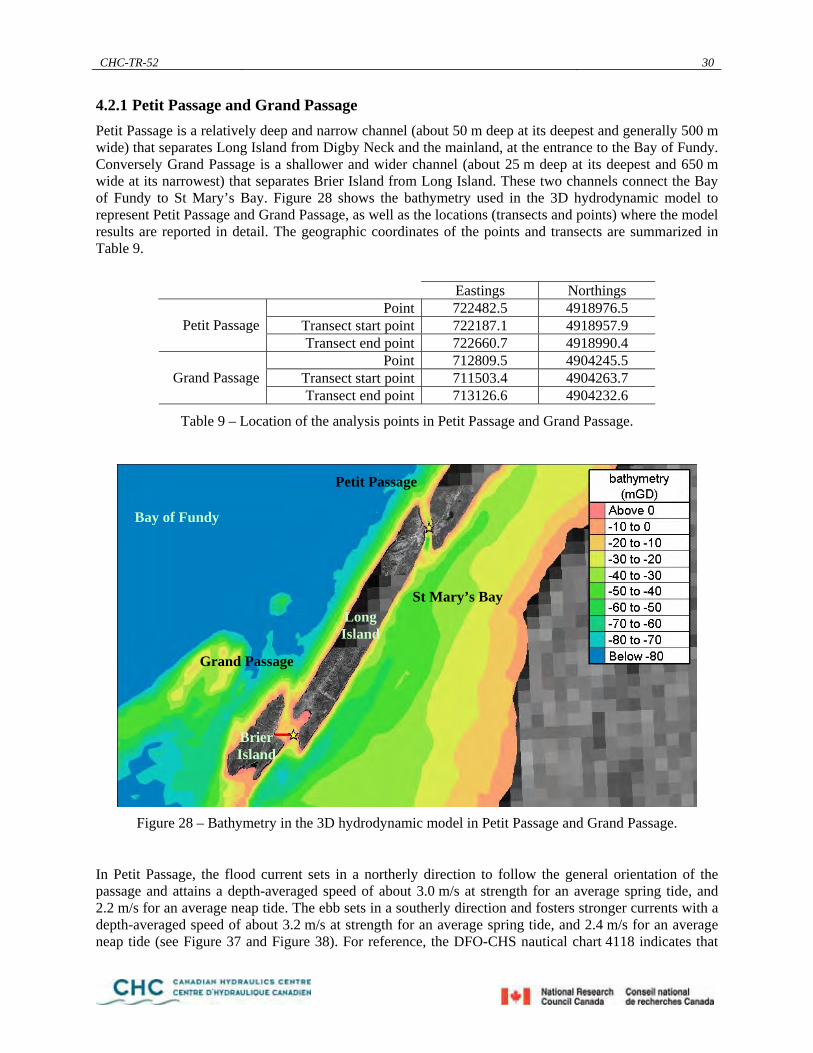
CHC-TR-52 30
4.2.1 Petit Passage and Grand Passage Petit Passage is a relatively deep and narrow channel (about 50 m deep at its deepest and generally 500 m wide) that separates Long Island from Digby Neck and the mainland, at the entrance to the Bay of Fundy. Conversely Grand Passage is a shallower and wider channel (about 25 m deep at its deepest and 650 m wide at its narrowest) that separates Brier Island from Long Island. These two channels connect the Bay of Fundy to St Mary’s Bay. Figure 28 shows the bathymetry used in the 3D hydrodynamic model to represent Petit Passage and Grand Passage, as well as the locations (transects and points) where the model results are reported in detail. The geographic coordinates of the points and transects are summarized in Table 9.
Eastings Northings
Point 722482.5 4918976.5 Transect start point 722187.1 4918957.9 Petit Passage Transect end point 722660.7 4918990.4
Point 712809.5 4904245.5 Transect start point 711503.4 4904263.7 Grand Passage Transect end point 713126.6 4904232.6
Table 9 – Location of the analysis points in Petit Passage and Grand Passage.
Figure 28 – Bathymetry in the 3D hydrodynamic model in Petit Passage and Grand Passage.
In Petit Passage, the flood current sets in a northerly direction to follow the general orientation of the passage and attains a depth-averaged speed of about 3.0 m/s at strength for an average spring tide, and 2.2 m/s for an average neap tide. The ebb sets in a southerly direction and fosters stronger currents with a depth-averaged speed of about 3.2 m/s at strength for an average spring tide, and 2.4 m/s for an average neap tide (see Figure 37 and Figure 38). For reference, the DFO-CHS nautical chart 4118 indicates that
Petit Passage
Grand Passage
St Mary’s Bay
Bay of Fundy
LongIsland
Brier Island
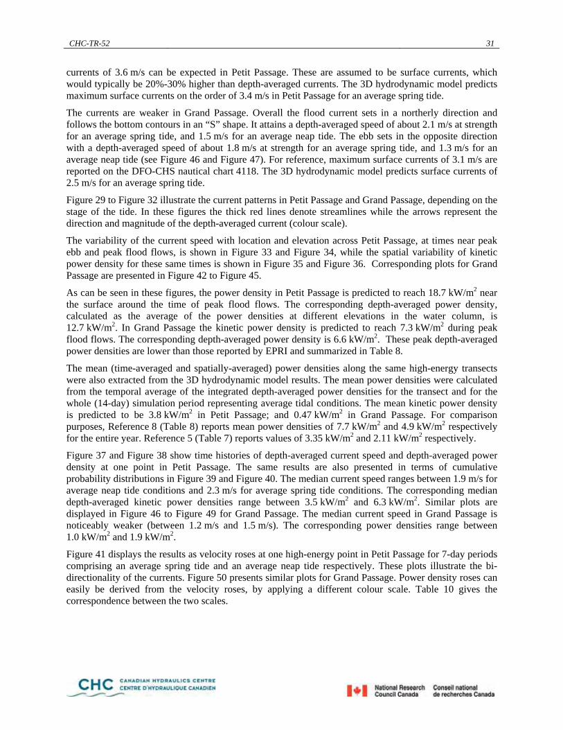
CHC-TR-52 31
currents of 3.6 m/s can be expected in Petit Passage. These are assumed to be surface currents, which would typically be 20%-30% higher than depth-averaged currents. The 3D hydrodynamic model predicts maximum surface currents on the order of 3.4 m/s in Petit Passage for an average spring tide.
The currents are weaker in Grand Passage. Overall the flood current sets in a northerly direction and follows the bottom contours in an “S” shape. It attains a depth-averaged speed of about 2.1 m/s at strength for an average spring tide, and 1.5 m/s for an average neap tide. The ebb sets in the opposite direction with a depth-averaged speed of about 1.8 m/s at strength for an average spring tide, and 1.3 m/s for an average neap tide (see Figure 46 and Figure 47). For reference, maximum surface currents of 3.1 m/s are reported on the DFO-CHS nautical chart 4118. The 3D hydrodynamic model predicts surface currents of 2.5 m/s for an average spring tide.
Figure 29 to Figure 32 illustrate the current patterns in Petit Passage and Grand Passage, depending on the stage of the tide. In these figures the thick red lines denote streamlines while the arrows represent the direction and magnitude of the depth-averaged current (colour scale).
The variability of the current speed with location and elevation across Petit Passage, at times near peak ebb and peak flood flows, is shown in Figure 33 and Figure 34, while the spatial variability of kinetic power density for these same times is shown in Figure 35 and Figure 36. Corresponding plots for Grand Passage are presented in Figure 42 to Figure 45.
As can be seen in these figures, the power density in Petit Passage is predicted to reach 18.7 kW/m2 near the surface around the time of peak flood flows. The corresponding depth-averaged power density, calculated as the average of the power densities at different elevations in the water column, is 12.7 kW/m2. In Grand Passage the kinetic power density is predicted to reach 7.3 kW/m2 during peak flood flows. The corresponding depth-averaged power density is 6.6 kW/m2. These peak depth-averaged power densities are lower than those reported by EPRI and summarized in Table 8.
The mean (time-averaged and spatially-averaged) power densities along the same high-energy transects were also extracted from the 3D hydrodynamic model results. The mean power densities were calculated from the temporal average of the integrated depth-averaged power densities for the transect and for the whole (14-day) simulation period representing average tidal conditions. The mean kinetic power density is predicted to be 3.8 kW/m2 in Petit Passage; and 0.47 kW/m2 in Grand Passage. For comparison purposes, Reference 8 (Table 8) reports mean power densities of 7.7 kW/m2 and 4.9 kW/m2 respectively for the entire year. Reference 5 (Table 7) reports values of 3.35 kW/m2 and 2.11 kW/m2 respectively.
Figure 37 and Figure 38 show time histories of depth-averaged current speed and depth-averaged power density at one point in Petit Passage. The same results are also presented in terms of cumulative probability distributions in Figure 39 and Figure 40. The median current speed ranges between 1.9 m/s for average neap tide conditions and 2.3 m/s for average spring tide conditions. The corresponding median depth-averaged kinetic power densities range between 3.5 kW/m2 and 6.3 kW/m2. Similar plots are displayed in Figure 46 to Figure 49 for Grand Passage. The median current speed in Grand Passage is noticeably weaker (between 1.2 m/s and 1.5 m/s). The corresponding power densities range between 1.0 kW/m2 and 1.9 kW/m2.
Figure 41 displays the results as velocity roses at one high-energy point in Petit Passage for 7-day periods comprising an average spring tide and an average neap tide respectively. These plots illustrate the bi-directionality of the currents. Figure 50 presents similar plots for Grand Passage. Power density roses can easily be derived from the velocity roses, by applying a different colour scale. Table 10 gives the correspondence between the two scales.

CHC-TR-52 32
Colour scale for
velocity rose Colour scale for
power density rose above 3.00 m/s above 13.8 kW/m2 above 2.75 m/s above 10.7 kW/m2 above 2.50 m/s above 8.0 kW/m2 above 2.00 m/s above 4.1 kW/m2 above 1.50 m/s above 1.7 kW/m2 above 1.00 m/s above 0.51 kW/m2
Table 10 – Colour scale for power density roses in Petit and Grand Passages.
Figure 51 and Figure 53 show the spatial variation in predicted depth-averaged mean currents in and around Petit Passage and Grand Passage for 7-day periods including an average spring tide and an average neap tide, respectively. Figure 52 and Figure 54 present the predicted depth-averaged maximum currents. Finally, Figure 55 to Figure 58 show the mean and maximum depth-averaged power densities throughout the region for average spring and neap tide conditions.
Figure 29 – Flow pathways predicted by the 3D hydrodynamic model in Petit Passage and Grand Passage
near high water.
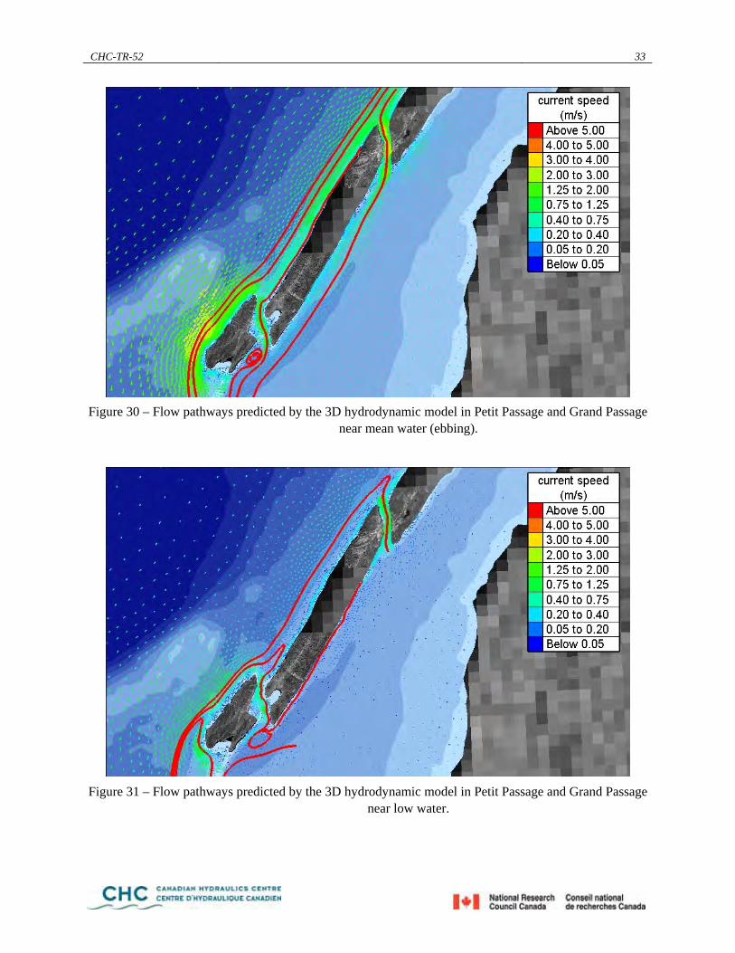
CHC-TR-52 33
Figure 30 – Flow pathways predicted by the 3D hydrodynamic model in Petit Passage and Grand Passage
near mean water (ebbing).
Figure 31 – Flow pathways predicted by the 3D hydrodynamic model in Petit Passage and Grand Passage
near low water.

CHC-TR-52 34
Figure 32 – Flow pathways predicted by the 3D hydrodynamic model in Petit Passage and Grand Passage
near mean water (flooding).
Figure 33 – Vertical cross-sections of three-dimensional current speed predicted by the 3D hydrodynamic
model in Petit Passage (near peak ebb flow).

CHC-TR-52 35
Figure 34 – Vertical cross-sections of three-dimensional current speed predicted by the 3D hydrodynamic
model in Petit Passage (near peak flood flow).
Figure 35 – Vertical cross-sections of three-dimensional power density predicted by the 3D
hydrodynamic model in Petit Passage (near peak ebb flow).

CHC-TR-52 36
Figure 36 – Vertical cross-sections of three-dimensional power density predicted by the 3D
hydrodynamic model in Petit Passage (near peak flood flow).

CHC-TR-52 37
0.0
0.5
1.0
1.5
2.0
2.5
3.0
3.5
4.0
0 1 2 3 4 5 6 7Days
curr
ent s
peed
(m/s
)
0.0
0.5
1.0
1.5
2.0
2.5
3.0
3.5
4.0Petit Passage - Predicted result
a)
0.0
2.0
4.0
6.0
8.0
10.0
12.0
14.0
16.0
18.0
20.0
0 1 2 3 4 5 6 7Days
pow
er d
ensi
ty (k
W/m
2 )
0.0
2.0
4.0
6.0
8.0
10.0
12.0
14.0
16.0
18.0
20.0Petit Passage - Predicted result
b)
Figure 37 – Time histories of a) depth-averaged current speed and b) depth-averaged power density predicted by the 3D hydrodynamic model in Petit Passage (average spring tide).

CHC-TR-52 38
0.0
0.5
1.0
1.5
2.0
2.5
3.0
3.5
4.0
0 1 2 3 4 5 6 7Days
curr
ent s
peed
(m/s
)
0.0
0.5
1.0
1.5
2.0
2.5
3.0
3.5
4.0Petit Passage - Predicted result
a)
0.0
2.0
4.0
6.0
8.0
10.0
12.0
14.0
16.0
18.0
20.0
0 1 2 3 4 5 6 7Days
pow
er d
ensi
ty (k
W/m
2 )
0.0
2.0
4.0
6.0
8.0
10.0
12.0
14.0
16.0
18.0
20.0Petit Passage - Predicted result
b)
Figure 38 – Time histories of a) depth-averaged current speed and b) depth-averaged power density predicted by the 3D hydrodynamic model in Petit Passage (average neap tide).
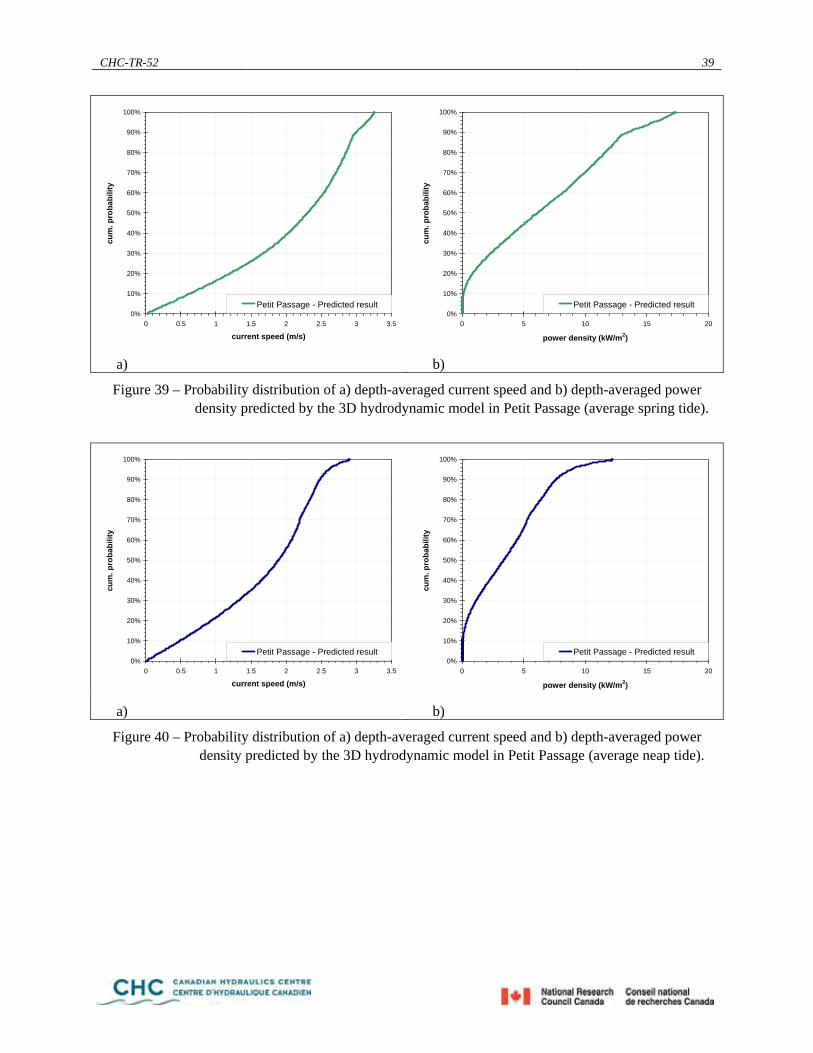
CHC-TR-52 39
0%
10%
20%
30%
40%
50%
60%
70%
80%
90%
100%
0 0.5 1 1.5 2 2.5 3 3.5
current speed (m/s)
cum
. pro
babi
lity
Petit Passage - Predicted result
0%
10%
20%
30%
40%
50%
60%
70%
80%
90%
100%
0 5 10 15 20
power density (kW/m2)
cum
. pro
babi
lity
Petit Passage - Predicted result
a) b)
Figure 39 – Probability distribution of a) depth-averaged current speed and b) depth-averaged power density predicted by the 3D hydrodynamic model in Petit Passage (average spring tide).
0%
10%
20%
30%
40%
50%
60%
70%
80%
90%
100%
0 0.5 1 1.5 2 2.5 3 3.5
current speed (m/s)
cum
. pro
babi
lity
Petit Passage - Predicted result
0%
10%
20%
30%
40%
50%
60%
70%
80%
90%
100%
0 5 10 15 20
power density (kW/m2)
cum
. pro
babi
lity
Petit Passage - Predicted result
a) b)
Figure 40 – Probability distribution of a) depth-averaged current speed and b) depth-averaged power density predicted by the 3D hydrodynamic model in Petit Passage (average neap tide).

CHC-TR-52 40
a) b)
Figure 41 – Roses of depth-averaged current speed predicted by the 3D hydrodynamic model in Petit Passage ( a) average spring tide and b) average neap tide).
Figure 42 – Vertical cross-sections of three-dimensional current speed predicted by the 3D hydrodynamic
model in Grand Passage (near peak ebb flow).

CHC-TR-52 41
Figure 43 – Vertical cross-sections of three-dimensional current speed predicted by the 3D hydrodynamic
model in Grand Passage (near peak flood flow).
Figure 44 – Vertical cross-sections of three-dimensional power density predicted by the 3D
hydrodynamic model in Grand Passage (near peak ebb flow).
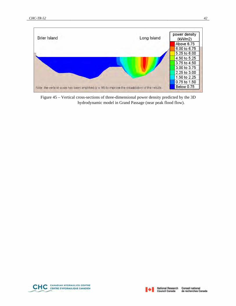
CHC-TR-52 42
Figure 45 – Vertical cross-sections of three-dimensional power density predicted by the 3D
hydrodynamic model in Grand Passage (near peak flood flow).

CHC-TR-52 43
0.0
0.5
1.0
1.5
2.0
2.5
3.0
0 1 2 3 4 5 6 7Days
curr
ent s
peed
(m/s
)
0.0
0.5
1.0
1.5
2.0
2.5
3.0Grand Passage - Predicted result
a)
0.0
1.0
2.0
3.0
4.0
5.0
6.0
7.0
8.0
0 1 2 3 4 5 6 7Days
pow
er d
ensi
ty (k
W/m
2 )
0.0
1.0
2.0
3.0
4.0
5.0
6.0
7.0
8.0Grand Passage - Predicted result
b)
Figure 46 – Time histories of a) depth-averaged current speed and b) depth-averaged power density predicted by the 3D hydrodynamic model in Grand Passage (average spring tide).
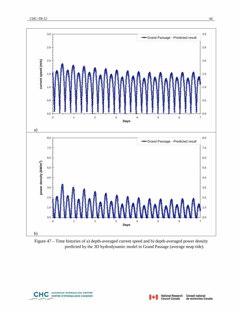
CHC-TR-52 44
0.0
0.5
1.0
1.5
2.0
2.5
3.0
0 1 2 3 4 5 6 7Days
curr
ent s
peed
(m/s
)
0.0
0.5
1.0
1.5
2.0
2.5
3.0Grand Passage - Predicted result
a)
0.0
1.0
2.0
3.0
4.0
5.0
6.0
7.0
8.0
0 1 2 3 4 5 6 7Days
pow
er d
ensi
ty (k
W/m
2 )
0.0
1.0
2.0
3.0
4.0
5.0
6.0
7.0
8.0Grand Passage - Predicted result
b)
Figure 47 – Time histories of a) depth-averaged current speed and b) depth-averaged power density predicted by the 3D hydrodynamic model in Grand Passage (average neap tide).

CHC-TR-52 45
0%
10%
20%
30%
40%
50%
60%
70%
80%
90%
100%
0 0.5 1 1.5 2 2.5
current speed (m/s)
cum
. pro
babi
lity
Grand Passage - Predicted result
0%
10%
20%
30%
40%
50%
60%
70%
80%
90%
100%
0 1 2 3 4 5 6
power density (kW/m2)
cum
. pro
babi
lity
Grand Passage - Predicted result
a) b)
Figure 48 – Probability distribution of a) depth-averaged current speed and b) depth-averaged power density predicted by the 3D hydrodynamic model in Grand Passage (average spring tide).
0%
10%
20%
30%
40%
50%
60%
70%
80%
90%
100%
0 0.5 1 1.5 2 2.5
current speed (m/s)
cum
. pro
babi
lity
Grand Passage - Predicted result
0%
10%
20%
30%
40%
50%
60%
70%
80%
90%
100%
0 1 2 3 4 5 6
power density (kW/m2)
cum
. pro
babi
lity
Grand Passage - Predicted result
a) b)
Figure 49 – Probability distribution of a) depth-averaged current speed and b) depth-averaged power density predicted by the 3D hydrodynamic model in Grand Passage (average neap tide).

CHC-TR-52 46
a) b)
Figure 50 – Roses of depth-averaged current speed predicted by the 3D hydrodynamic model in Grand Passage ( a) average spring tide and b) average neap tide).
Figure 51 – Depth-averaged mean currents predicted by the 3D hydrodynamic model in Petit Passage and
Grand Passage (average spring tide).
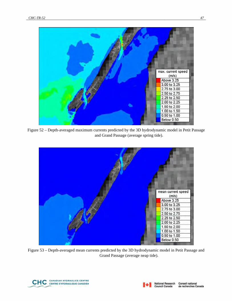
CHC-TR-52 47
Figure 52 – Depth-averaged maximum currents predicted by the 3D hydrodynamic model in Petit Passage
and Grand Passage (average spring tide).
Figure 53 – Depth-averaged mean currents predicted by the 3D hydrodynamic model in Petit Passage and
Grand Passage (average neap tide).

CHC-TR-52 48
Figure 54 – Depth-averaged maximum currents predicted by the 3D hydrodynamic model in Petit Passage
and Grand Passage (average neap tide).
Figure 55 – Depth-averaged mean power density predicted by the 3D hydrodynamic model in Petit
Passage and Grand Passage (average spring tide).
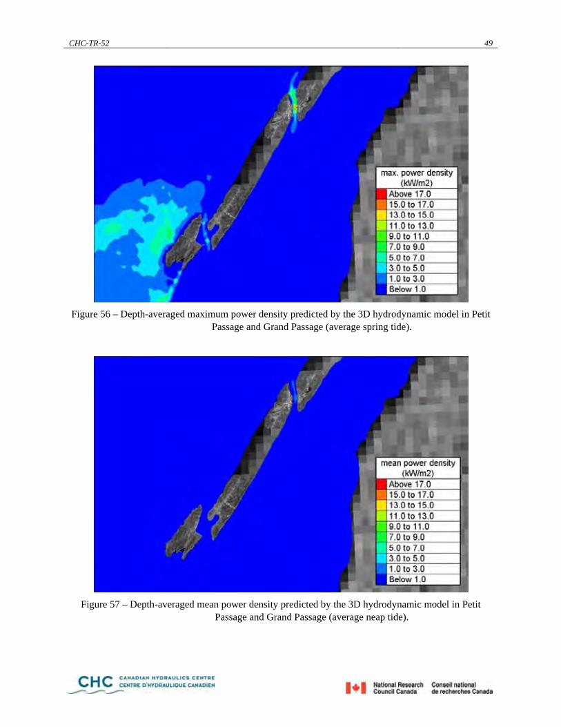
CHC-TR-52 49
Figure 56 – Depth-averaged maximum power density predicted by the 3D hydrodynamic model in Petit
Passage and Grand Passage (average spring tide).
Figure 57 – Depth-averaged mean power density predicted by the 3D hydrodynamic model in Petit
Passage and Grand Passage (average neap tide).
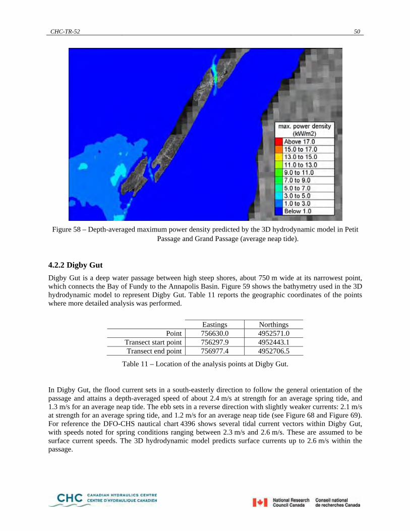
CHC-TR-52 50
Figure 58 – Depth-averaged maximum power density predicted by the 3D hydrodynamic model in Petit
Passage and Grand Passage (average neap tide).
4.2.2 Digby Gut Digby Gut is a deep water passage between high steep shores, about 750 m wide at its narrowest point, which connects the Bay of Fundy to the Annapolis Basin. Figure 59 shows the bathymetry used in the 3D hydrodynamic model to represent Digby Gut. Table 11 reports the geographic coordinates of the points where more detailed analysis was performed.
Eastings Northings
Point 756630.0 4952571.0 Transect start point 756297.9 4952443.1 Transect end point 756977.4 4952706.5
Table 11 – Location of the analysis points at Digby Gut.
In Digby Gut, the flood current sets in a south-easterly direction to follow the general orientation of the passage and attains a depth-averaged speed of about 2.4 m/s at strength for an average spring tide, and 1.3 m/s for an average neap tide. The ebb sets in a reverse direction with slightly weaker currents: 2.1 m/s at strength for an average spring tide, and 1.2 m/s for an average neap tide (see Figure 68 and Figure 69). For reference the DFO-CHS nautical chart 4396 shows several tidal current vectors within Digby Gut, with speeds noted for spring conditions ranging between 2.3 m/s and 2.6 m/s. These are assumed to be surface current speeds. The 3D hydrodynamic model predicts surface currents up to 2.6 m/s within the passage.

CHC-TR-52 51
Figure 59 – Bathymetry in the 3D hydrodynamic model at Digby Gut.
The variability of the current speed with location and elevation across Digby Gut, at times near peak ebb and peak flood flows, is shown in Figure 64 and Figure 65, while the spatial variation of kinetic power density for these same times is shown in Figure 66 and Figure 67. The location of the transect is shown as a thick red line in Figure 59. The kinetic power density at Digby Gut is predicted to reach 4.5 kW/m2 near the surface during peak ebb flows. The corresponding depth-averaged power density, calculated as the average of the power densities predicted at different elevations in the water column, is 4.2 kW/m2. These peak kinetic power density values are similar to those predicted by EPRI and presented in Table 8.
The mean kinetic power density along the same high-energy transect was also derived from the temporal average of the integrated depth-averaged power densities for the whole (14-day) simulation period representing average tidal conditions. The mean kinetic power density in Digby Gut is predicted to be 0.94 kW/m2. This value can be compared to EPRI’s estimate of 1.8 kW/m2 for the entire year (see Table 8 and Reference 8); and to the mean power density of 1.22 kW/m2 reported in Reference 5 at Digby Gut.
Figure 68 and Figure 69 show time histories of depth-averaged current speed and depth-averaged power density at one point in Digby Gut. This point is shown as a yellow star in Figure 59. The same results are also presented in terms of cumulative probability distribution in Figure 70 and Figure 71. The median depth-averaged current speed at this location is 0.9 m/s for average neap conditions and 1.3 m/s for average spring conditions. The corresponding median depth-averaged kinetic power densities range between 0.4 kW/m2 and 1.1 kW/m2.
The simulation results at this location are also presented in Figure 72 in the form of velocity roses for two 7-day periods corresponding to an average spring tide and an average neap tide respectively. These plots demonstrate the bi-directionality of the currents at Digby Gut, which is to be expected given the configuration of the passage. Power density roses can easily be derived from the velocity roses, by applying a different colour scale. Table 12 gives the correspondence between the two scales.
Digby Gut
Annapolis Basin
towards Hampton
towards Sandy Cove
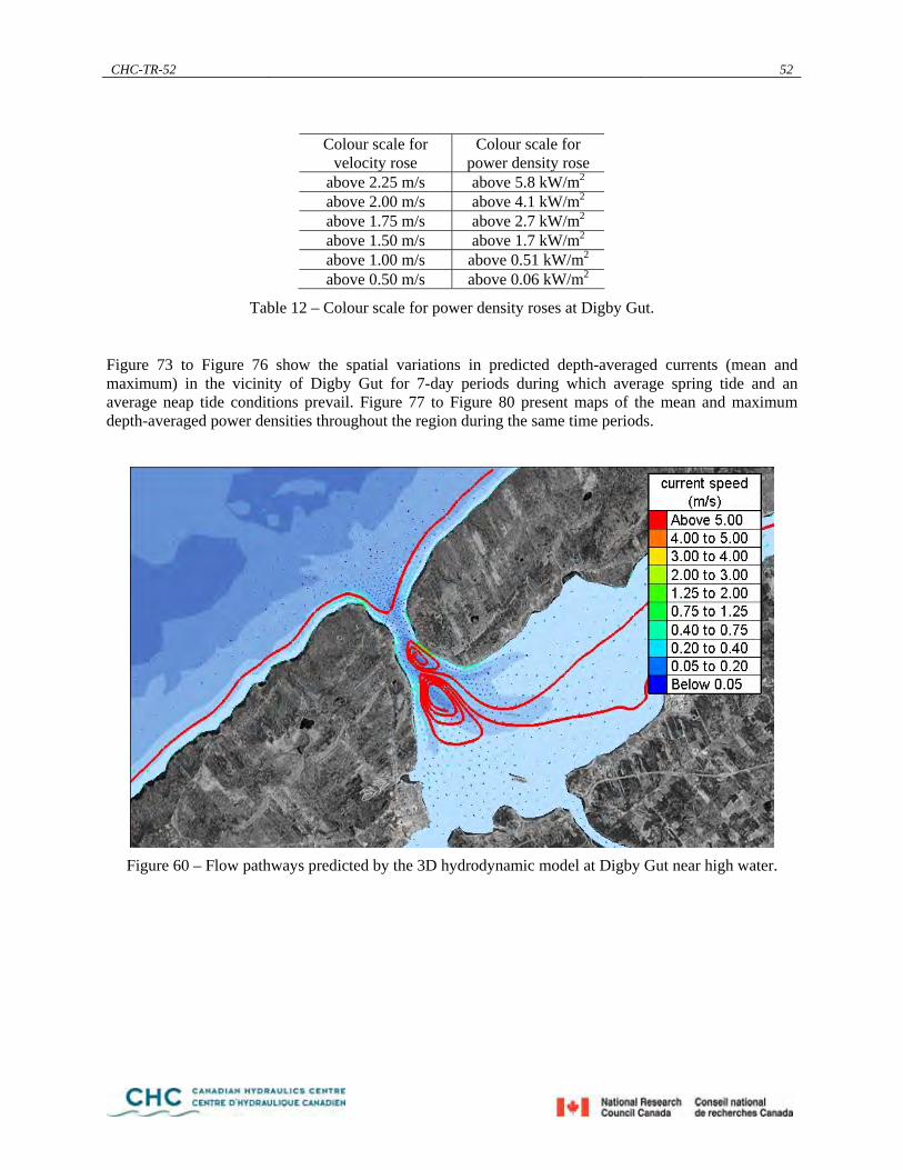
CHC-TR-52 52
Colour scale for
velocity rose Colour scale for
power density rose above 2.25 m/s above 5.8 kW/m2 above 2.00 m/s above 4.1 kW/m2 above 1.75 m/s above 2.7 kW/m2 above 1.50 m/s above 1.7 kW/m2 above 1.00 m/s above 0.51 kW/m2 above 0.50 m/s above 0.06 kW/m2
Table 12 – Colour scale for power density roses at Digby Gut.
Figure 73 to Figure 76 show the spatial variations in predicted depth-averaged currents (mean and maximum) in the vicinity of Digby Gut for 7-day periods during which average spring tide and an average neap tide conditions prevail. Figure 77 to Figure 80 present maps of the mean and maximum depth-averaged power densities throughout the region during the same time periods.
Figure 60 – Flow pathways predicted by the 3D hydrodynamic model at Digby Gut near high water.

CHC-TR-52 53
Figure 61 – Flow pathways predicted by the 3D hydrodynamic model at Digby Gut near mean water
(ebbing).
Figure 62 – Flow pathways predicted by the 3D hydrodynamic model at Digby Gut near low water.

CHC-TR-52 54
Figure 63 – Flow pathways predicted by the 3D hydrodynamic model at Digby Gut near mean water
(flooding).
Figure 64 – Vertical cross-sections of three-dimensional current speed predicted by the 3D hydrodynamic
model at Digby Gut (near peak ebb flow).

CHC-TR-52 55
Figure 65 – Vertical cross-sections of three-dimensional current speed predicted by the 3D hydrodynamic
model at Digby Gut (near peak flood flow).
Figure 66 – Vertical cross-sections of three-dimensional power density predicted by the 3D
hydrodynamic model at Digby Gut (near peak ebb flow).
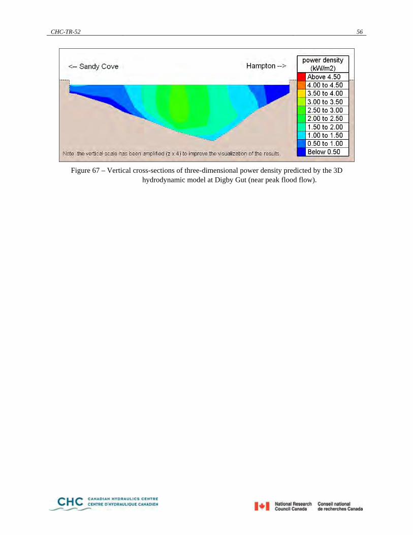
CHC-TR-52 56
Figure 67 – Vertical cross-sections of three-dimensional power density predicted by the 3D
hydrodynamic model at Digby Gut (near peak flood flow).

CHC-TR-52 57
0.0
0.5
1.0
1.5
2.0
2.5
3.0
0 1 2 3 4 5 6 7Days
curr
ent s
peed
(m/s
)
0.0
0.5
1.0
1.5
2.0
2.5
3.0Digby Gut - Predicted result
a)
0.0
1.0
2.0
3.0
4.0
5.0
6.0
7.0
8.0
9.0
0 1 2 3 4 5 6 7Days
pow
er d
ensi
ty (k
W/m
2 )
0.0
1.0
2.0
3.0
4.0
5.0
6.0
7.0
8.0
9.0Digby Gut - Predicted result
b)
Figure 68 – Time histories of a) depth-averaged current speed and b) depth-averaged power density predicted by the 3D hydrodynamic model at Digby Gut (average spring tide).
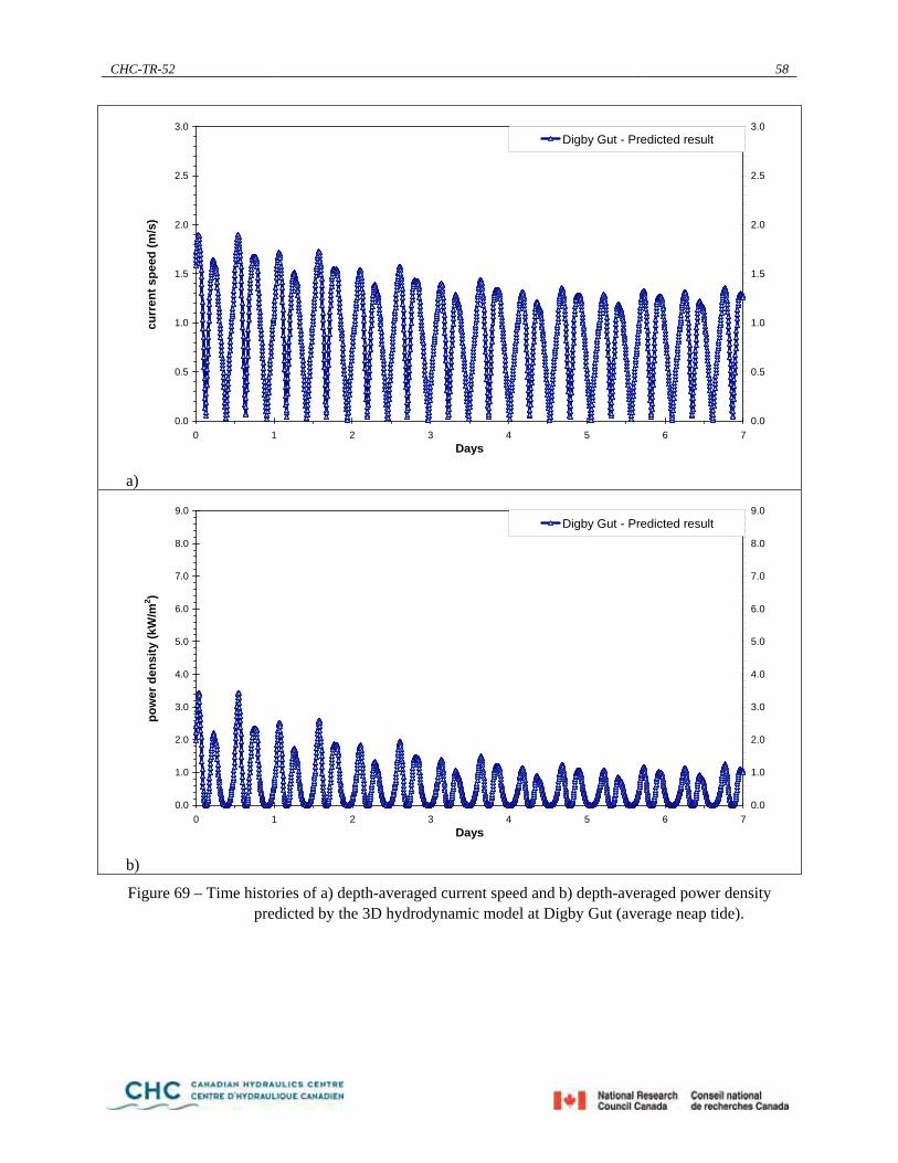
CHC-TR-52 58
0.0
0.5
1.0
1.5
2.0
2.5
3.0
0 1 2 3 4 5 6 7Days
curr
ent s
peed
(m/s
)
0.0
0.5
1.0
1.5
2.0
2.5
3.0Digby Gut - Predicted result
a)
0.0
1.0
2.0
3.0
4.0
5.0
6.0
7.0
8.0
9.0
0 1 2 3 4 5 6 7Days
pow
er d
ensi
ty (k
W/m
2 )
0.0
1.0
2.0
3.0
4.0
5.0
6.0
7.0
8.0
9.0Digby Gut - Predicted result
b)
Figure 69 – Time histories of a) depth-averaged current speed and b) depth-averaged power density predicted by the 3D hydrodynamic model at Digby Gut (average neap tide).

CHC-TR-52 59
0%
10%
20%
30%
40%
50%
60%
70%
80%
90%
100%
0 0.5 1 1.5 2 2.5 3
current speed (m/s)
cum
. pro
babi
lity
Digby Gut - Predicted result
0%
10%
20%
30%
40%
50%
60%
70%
80%
90%
100%
0 1 2 3 4 5 6 7 8
power density (kW/m2)
cum
. pro
babi
lity
Digby Gut - Predicted result
a) b)
Figure 70 – Probability distribution of a) depth-averaged current speed and b) depth-averaged power density predicted by the 3D hydrodynamic model at Digby Gut (average spring tide).
0%
10%
20%
30%
40%
50%
60%
70%
80%
90%
100%
0 0.5 1 1.5 2 2.5 3
current speed (m/s)
cum
. pro
babi
lity
Digby Gut - Predicted result
0%
10%
20%
30%
40%
50%
60%
70%
80%
90%
100%
0 1 2 3 4 5 6 7 8
power density (kW/m2)
cum
. pro
babi
lity
Digby Gut - Predicted result
a) b)
Figure 71 – Probability distribution of a) depth-averaged current speed and b) depth-averaged power density predicted by the 3D hydrodynamic model at Digby Gut (average neap tide).

CHC-TR-52 60
a) b)
Figure 72 – Roses of depth-averaged current speed predicted by the 3D hydrodynamic model at Digby Gut ( a) average spring tide and b) average neap tide).
Figure 73 – Depth-averaged mean currents predicted by the 3D hydrodynamic model at Digby Gut
(average spring tide).

CHC-TR-52 61
Figure 74 – Depth-averaged maximum currents predicted by the 3D hydrodynamic model at Digby Gut
(average spring tide).
Figure 75 – Depth-averaged mean currents predicted by the 3D hydrodynamic model at Digby Gut
(average neap tide).

CHC-TR-52 62
Figure 76 – Depth-averaged maximum currents predicted by the 3D hydrodynamic model at Digby Gut
(average neap tide).
Figure 77 – Depth-averaged mean power density predicted by the 3D hydrodynamic model at Digby Gut
(average spring tide).

CHC-TR-52 63
Figure 78 – Depth-averaged maximum power density predicted by the 3D hydrodynamic model at Digby
Gut (average spring tide).
Figure 79 – Depth-averaged mean power density predicted by the 3D hydrodynamic model at Digby Gut
(average neap tide).

CHC-TR-52 64
Figure 80 – Depth-averaged maximum power density predicted by the 3D hydrodynamic model at Digby
Gut (average neap tide).
4.2.3 Minas Passage Minas Passage is a wide and deep channel (about 160 m deep at its deepest and generally 5 km wide) between Cape Split and Parrsboro Harbour that connects Minas Channel to Minas Basin, near the head of the Bay of Fundy. Figure 81 shows the bathymetry used in the 3D hydrodynamic model to represent Minas Channel, Minas Passage and Minas Basin, as well as the locations (transect and point) where the simulation results are presented and discussed in greater detail in what follows. The geographic coordinates of the points and transects are summarized in Table 13.
Eastings Northings
Point 851787.0 5031591.0 Transect start point 851876.5 5030051.8 Transect end point 851651.1 5036185.3
Table 13 – Location of the analysis points in Minas Passage.
In Minas Channel, the flood current sets in a north-easterly direction abreast the southern shores until it reaches Long Beach, at which point the flood sets strongly northward towards Cape Split. Its direction then changes again strongly to follow the general orientation of Minas Passage (easterly). The ebb generally sets in a reverse direction although the changes in direction are less sharp and pronounced. As a result the ebb current generally flows along the northern shores.

CHC-TR-52 65
Figure 81 – 3D hydrodynamic model bathymetry in Minas Channel and Minas Passage.
There are strong recirculation patterns worth noting in Minas Channel and Minas Passage, as illustrated by streamlines (thick red lines) in Figure 82 to Figure 85. It should be remembered that streamlines are lines tangent at any point to the currents. They offer a visual indication of the flow pathways. With flooding comes turbulence in the lee of Cape Split and near Parrsboro Harbour. At high water eddies form in the passage. Large eddies then develop in Scots Bay, south of Cape Split, when the water is retreating on ebb flows. The eddies are widest at low water. The current patterns predicted by the new 3D hydrodynamic model are consistent with those predicted in the Atlas of Tidal Currents for the Bay of Fundy published by the Canadian Hydrographic Service (Reference 16).
The flood current in Minas Passage attains a depth-averaged speed of about 4.1 m/s at strength in the middle of the channel for an average spring tide, and 3.0 m/s for an average neap tide. The ebb current reaches a depth-averaged speed of about 4.3 m/s at strength for an average spring tide, and 2.8 m/s for an average neap tide (see Figure 90 and Figure 91). For reference, maximum surface currents of 4.1 m/s are reported on DFO-CHS nautical chart 4399. The 3D hydrodynamic model predicts maximum surface current speeds on the order of 5.0 m/s in Minas Passage for an average spring tide. Even stronger currents should be expected during an extreme spring tide.
The variability of the current speed with location and elevation along the transect denoted by a thick red line in Figure 81, at times near peak ebb and peak flood flows, is plotted in Figure 86 and Figure 87, while the spatial variability of kinetic power density over this cross-section for these same times is mapped in Figure 88 and Figure 89. These figures show that the kinetic power density in Minas Passage reaches up to 77.8 kW/m2 during the peak ebb flows associated with an average spring tide. The corresponding depth-averaged power density, calculated as the average of the power densities predicted at different elevations in the water column is 69.5 kW/m2. This estimate of peak depth-averaged power density is significantly greater than that predicted by EPRI and summarized in Table 8.
Port Greville
Minas Channel
Cape Split
ParrsboroHarbour
Minas Passage

CHC-TR-52 66
The mean kinetic power density along the same high-energy transect was also derived as the temporal average of the integrated depth-averaged power densities over the whole (14-day) simulation period representing average tidal conditions. The mean kinetic power density for the selected transect is predicted to be 6.7 kW/m2. For comparison purposes, the EPRI study (Reference 8 and Table 8) estimated a mean power density of 4.9 kW/m2 for the entire year at Minas Passage. On the other hand, CHC-TR-41 (Reference 5 and Table 7) reported a power density of 6.04 kW/m2 for Minas Passage.
Time histories of depth-averaged current speed and depth-averaged power density at one high-energy point in Minas Passage (denoted by a yellow star in Figure 81) are displayed in Figure 90 and Figure 91. Cumulative probability distributions were derived from these time histories and are presented in Figure 92 and Figure 93 for average spring and average neap conditions. The median current speed at this high-energy point ranges between 2.3 m/s for average neap tide conditions and 3.0 m/s for average spring tide conditions. The corresponding median depth-averaged kinetic power density ranges between 6.0 kW/m2 and 13.6 kW/m2.
Figure 94 shows the simulation results displayed as velocity roses. It is clear from this figure that the flow direction during ebbing is not simply the reverse of the direction during flooding. However, the flow is mostly bi-directional at this point in Minas Passage. Power density roses can easily be derived from the velocity roses, by applying a different colour scale as given in Table 14.
Colour scale for
velocity rose Colour scale for
power density rose above 4.50 m/s above 46.7 kW/m2 above 4.00 m/s above 32.8 kW/m2 above 3.50 m/s above 22.0 kW/m2 above 3.00 m/s above 13.8 kW/m2 above 2.00 m/s above 4.1 kW/m2 above 1.00 m/s above 0.51 kW/m2
Table 14 – Colour scale for power density roses in Minas Passage.
Figure 95 and Figure 97 show the spatial variations in predicted depth-averaged mean currents in Minas Passage as filled colour contours for 7-day periods corresponding to an average spring tide and an average neap tide respectively. The maximum depth averaged current speeds during these 7-day periods are mapped in Figure 96 and Figure 98. It can be observed that there is a high energy spot near the tip of Cape Split where the currents are stronger than in the middle of the passage. This is corroborated by aerial photographs of Minas Basin (Reference 9) showing small waves and turbulence in this area. Figure 99 to Figure 102 show the mean maximum depth-averaged power densities throughout the region for average spring and neap tide conditions.
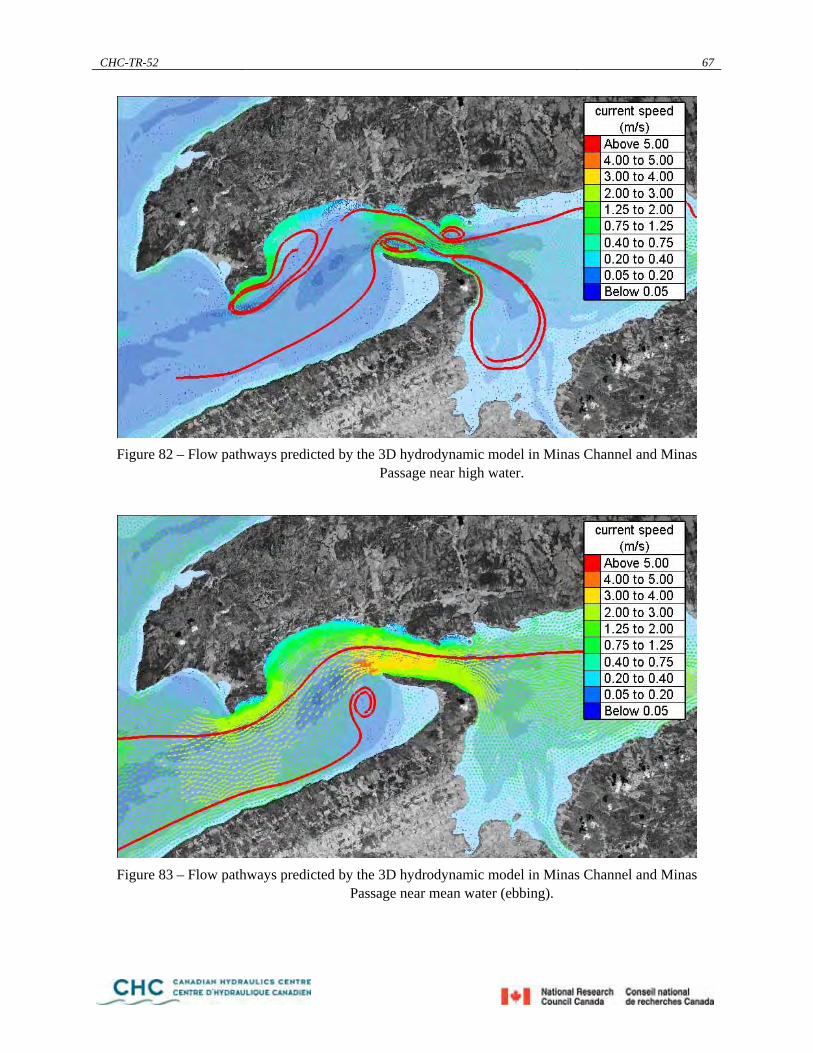
CHC-TR-52 67
Figure 82 – Flow pathways predicted by the 3D hydrodynamic model in Minas Channel and Minas
Passage near high water.
Figure 83 – Flow pathways predicted by the 3D hydrodynamic model in Minas Channel and Minas
Passage near mean water (ebbing).
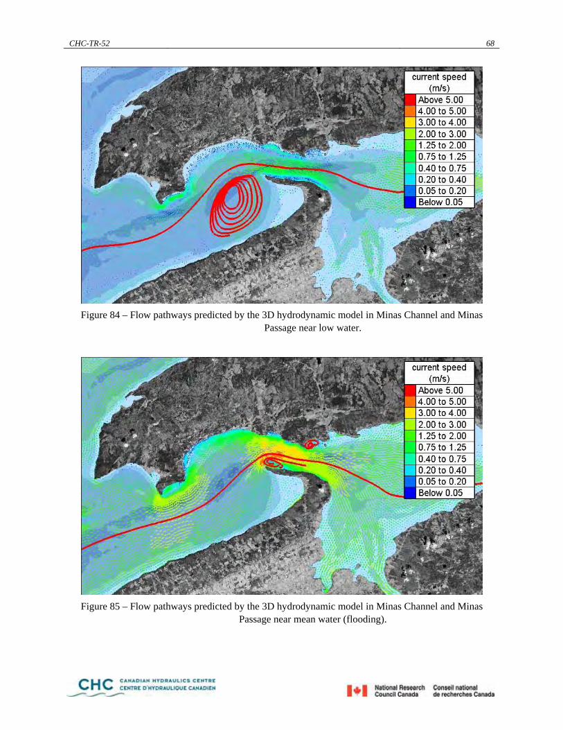
CHC-TR-52 68
Figure 84 – Flow pathways predicted by the 3D hydrodynamic model in Minas Channel and Minas
Passage near low water.
Figure 85 – Flow pathways predicted by the 3D hydrodynamic model in Minas Channel and Minas
Passage near mean water (flooding).
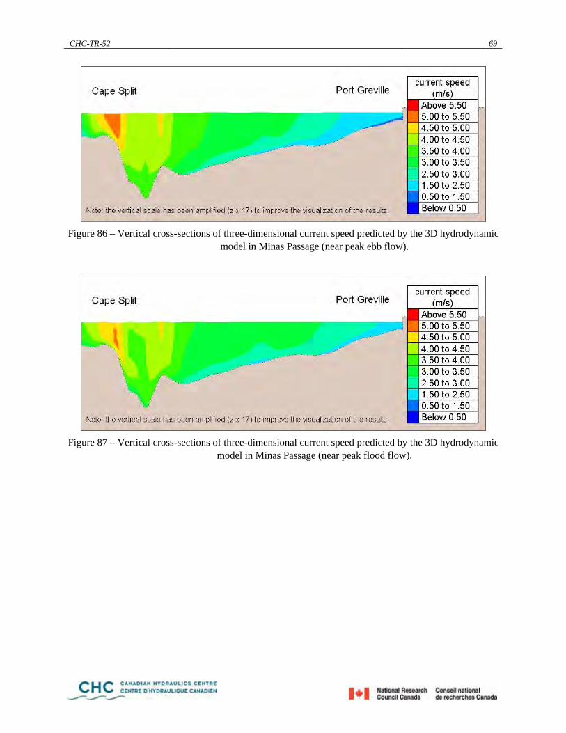
CHC-TR-52 69
Figure 86 – Vertical cross-sections of three-dimensional current speed predicted by the 3D hydrodynamic
model in Minas Passage (near peak ebb flow).
Figure 87 – Vertical cross-sections of three-dimensional current speed predicted by the 3D hydrodynamic
model in Minas Passage (near peak flood flow).

CHC-TR-52 70
Figure 88 – Vertical cross-sections of three-dimensional power density predicted by the 3D
hydrodynamic model in Minas Passage (near peak ebb flow).
Figure 89 – Vertical cross-sections of three-dimensional power density predicted by the 3D
hydrodynamic model in Minas Passage (near peak flood flow).

CHC-TR-52 71
0.0
0.5
1.0
1.5
2.0
2.5
3.0
3.5
4.0
4.5
5.0
0 1 2 3 4 5 6 7Days
curr
ent s
peed
(m/s
)
0.0
0.5
1.0
1.5
2.0
2.5
3.0
3.5
4.0
4.5
5.0Minas Passage - Predicted result
a)
0.0
5.0
10.0
15.0
20.0
25.0
30.0
35.0
40.0
45.0
50.0
0 1 2 3 4 5 6 7Days
pow
er d
ensi
ty (k
W/m
2 )
0.0
5.0
10.0
15.0
20.0
25.0
30.0
35.0
40.0
45.0
50.0Minas Passage - Predicted result
b)
Figure 90 – Time histories of a) depth-averaged current speed and b) depth-averaged power density predicted by the 3D hydrodynamic model in Minas Passage (average spring tide).
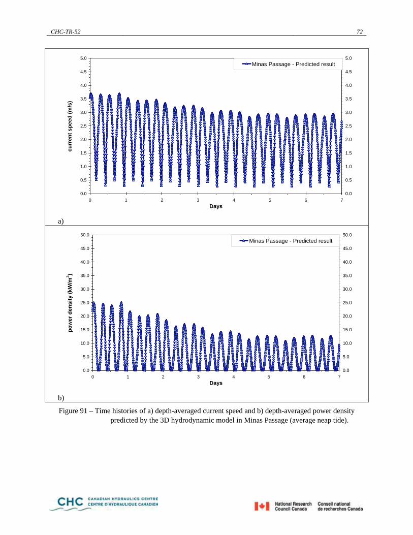
CHC-TR-52 72
0.0
0.5
1.0
1.5
2.0
2.5
3.0
3.5
4.0
4.5
5.0
0 1 2 3 4 5 6 7Days
curr
ent s
peed
(m/s
)
0.0
0.5
1.0
1.5
2.0
2.5
3.0
3.5
4.0
4.5
5.0Minas Passage - Predicted result
a)
0.0
5.0
10.0
15.0
20.0
25.0
30.0
35.0
40.0
45.0
50.0
0 1 2 3 4 5 6 7Days
pow
er d
ensi
ty (k
W/m
2 )
0.0
5.0
10.0
15.0
20.0
25.0
30.0
35.0
40.0
45.0
50.0Minas Passage - Predicted result
b)
Figure 91 – Time histories of a) depth-averaged current speed and b) depth-averaged power density predicted by the 3D hydrodynamic model in Minas Passage (average neap tide).

CHC-TR-52 73
0%
10%
20%
30%
40%
50%
60%
70%
80%
90%
100%
0 1 2 3 4 5
current speed (m/s)
cum
. pro
babi
lity
Minas Passage - Predicted result
0%
10%
20%
30%
40%
50%
60%
70%
80%
90%
100%
0 5 10 15 20 25 30 35 40 45
power density (kW/m2)
cum
. pro
babi
lity
Minas Passage - Predicted result
a) b)
Figure 92 – Probability distribution of a) depth-averaged current speed and b) depth-averaged power density predicted by the 3D hydrodynamic model in Minas Passage (average spring tide).
0%
10%
20%
30%
40%
50%
60%
70%
80%
90%
100%
0 1 2 3 4 5
current speed (m/s)
cum
. pro
babi
lity
Minas Passage - Predicted result
0%
10%
20%
30%
40%
50%
60%
70%
80%
90%
100%
0 5 10 15 20 25 30 35 40 45
power density (kW/m2)
cum
. pro
babi
lity
Minas Passage - Predicted result
a) b)
Figure 93 – Probability distribution of a) depth-averaged current speed and b) depth-averaged power density predicted by the 3D hydrodynamic model in Minas Passage (average neap tide).

CHC-TR-52 74
a) b)
Figure 94 – Roses of depth-averaged current speed predicted by the 3D hydrodynamic model in Minas Passage ( a) average spring tide and b) average neap tide).
Figure 95 – Depth-averaged mean currents predicted by the 3D hydrodynamic model in Minas Channel
and Minas Passage (average spring tide).

CHC-TR-52 75
Figure 96 – Depth-averaged maximum currents predicted by the 3D hydrodynamic model in Minas
Channel and Minas Passage (average spring tide).
Figure 97 – Depth-averaged mean currents predicted by the 3D hydrodynamic model in Minas Channel
and Minas Passage (average neap tide).
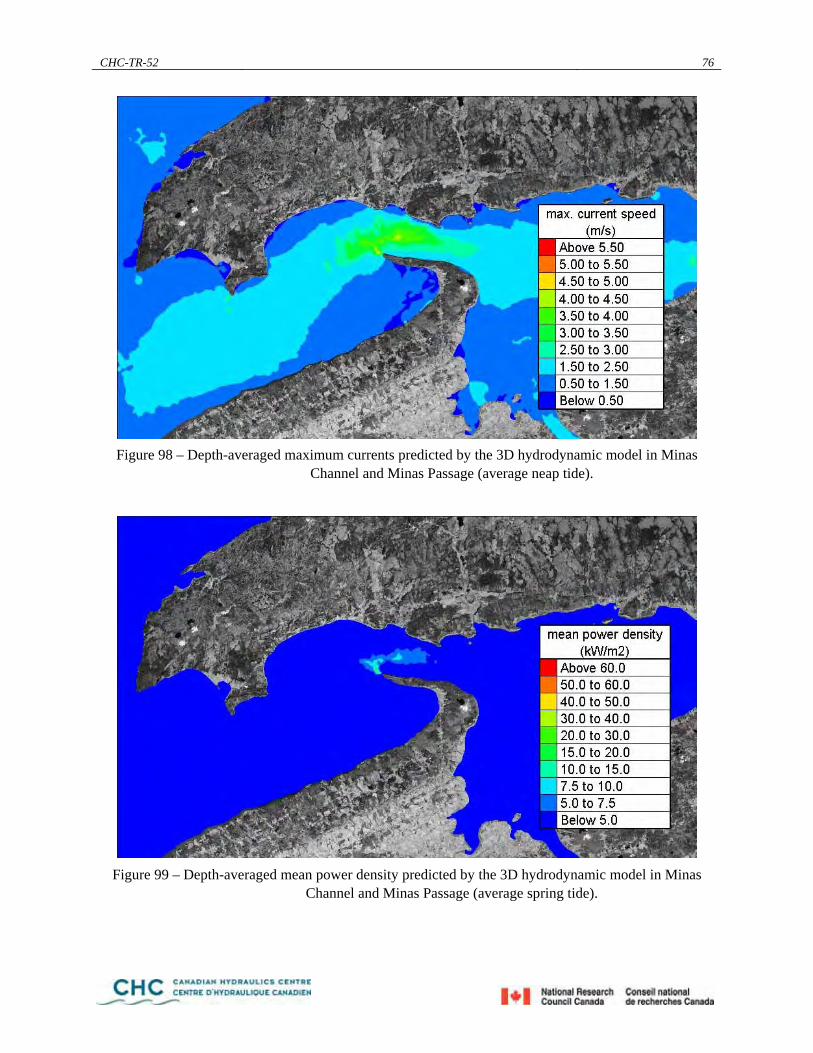
CHC-TR-52 76
Figure 98 – Depth-averaged maximum currents predicted by the 3D hydrodynamic model in Minas
Channel and Minas Passage (average neap tide).
Figure 99 – Depth-averaged mean power density predicted by the 3D hydrodynamic model in Minas
Channel and Minas Passage (average spring tide).

CHC-TR-52 77
Figure 100 – Depth-averaged maximum power density predicted by the 3D hydrodynamic model in
Minas Channel and Minas Passage (average spring tide).
Figure 101 – Depth-averaged mean power density predicted by the 3D hydrodynamic model in Minas
Channel and Minas Passage (average neap tide).

CHC-TR-52 78
Figure 102 – Depth-averaged maximum power density predicted by the 3D hydrodynamic model in
Minas Channel and Minas Passage (average neap tide).
4.3 Simulation Results for Selected Areas in New Brunswick The upper Bay of Fundy is known as home to some of the world’s largest tides. Three sites in New Brunswick were carefully studied to investigate their potential for tidal in-stream energy: Letete Passage, Western Passage and Head Harbour Passage at the entrance to Passamaquoddy Bay. The results specific to each area are presented in Sections 4.3.1, 4.3.2, and 4.3.3 respectively. Results pertaining to the entrance to Passamaquoddy Bay are presented below.
Figure 103 shows the bathymetry used in the 3D hydrodynamic model to represent the entrance to Passamaquoddy Bay, as well as the locations (transects and points) where the simulation results will be presented in more detail below.
Figure 104 to Figure 107 illustrate the flow pathways at the entrance to Passamaquoddy Bay for four different stages of the tide. In these figures the thick red lines are streamlines, which are lines tangent at any point to the currents. The arrows represent the current direction and magnitude. It is apparent from these figures that the current patterns are relatively smooth when the tide is running. However, numerous whirlpools and eddies develop at times of slack currents near high and low water.
Old Sow, the largest tidal whirlpool in the Western Hemisphere and one of five significant whirlpools worldwide, occurs in Western Passage, between Deer Island, NB, and Moose Island, USA. Old Sow is surrounded by numerous small and medium whirlpools, which results in an area with a diameter estimated at 75 metres. The currents are reported to be worst 3 hours after low water (Reference 17).
Figure 108 and Figure 110 display the spatial variations in predicted depth-averaged mean currents for the area as filled colour contours for 7-day periods including an average spring tide and an average neap tide respectively. The maximum depth-averaged currents during these 7-day periods are mapped in Figure 109 and Figure 111. These figures show stronger currents in the approaches to Letete Passage than anywhere
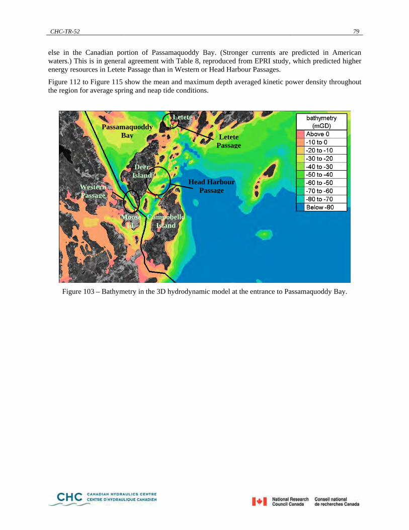
CHC-TR-52 79
else in the Canadian portion of Passamaquoddy Bay. (Stronger currents are predicted in American waters.) This is in general agreement with Table 8, reproduced from EPRI study, which predicted higher energy resources in Letete Passage than in Western or Head Harbour Passages.
Figure 112 to Figure 115 show the mean and maximum depth averaged kinetic power density throughout the region for average spring and neap tide conditions.
Figure 103 – Bathymetry in the 3D hydrodynamic model at the entrance to Passamaquoddy Bay.
Letete Passage
Western Passage
Head HarbourPassage
Passamaquoddy Bay
Deer Island
CampobelloIsland
Moose Id.
Letete

CHC-TR-52 80
Figure 104 – Flow pathways predicted by the 3D hydrodynamic model at the entrance to Passamaquoddy
Bay near high water.
Figure 105 – Flow pathways predicted by the 3D hydrodynamic model at the entrance to Passamaquoddy
Bay near mean water (ebbing).

CHC-TR-52 81
Figure 106 – Flow pathways predicted by the 3D hydrodynamic model at the entrance to Passamaquoddy
Bay near low water.
Figure 107 – Flow pathways predicted by the 3D hydrodynamic model at the entrance to Passamaquoddy
Bay near mean water (flooding).

CHC-TR-52 82
Figure 108 – Depth-averaged mean currents predicted by the 3D hydrodynamic model at the entrance to
Passamaquoddy Bay (average spring tide).
Figure 109 – Depth-averaged maximum currents predicted by the 3D hydrodynamic model at the entrance
to Passamaquoddy Bay (average spring tide).
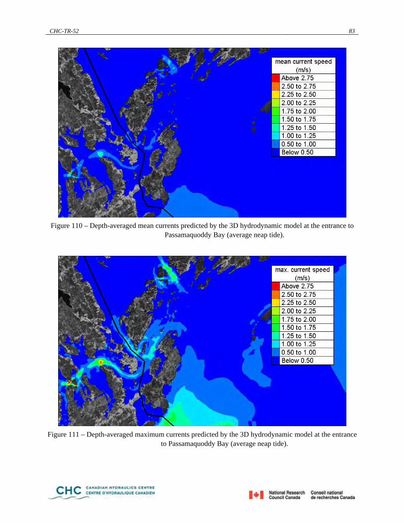
CHC-TR-52 83
Figure 110 – Depth-averaged mean currents predicted by the 3D hydrodynamic model at the entrance to
Passamaquoddy Bay (average neap tide).
Figure 111 – Depth-averaged maximum currents predicted by the 3D hydrodynamic model at the entrance
to Passamaquoddy Bay (average neap tide).

CHC-TR-52 84
Figure 112 – Depth-averaged mean power density predicted by the 3D hydrodynamic model at the
entrance to Passamaquoddy Bay (average spring tide).
Figure 113 – Depth-averaged maximum power density predicted by the 3D hydrodynamic model at the
entrance to Passamaquoddy Bay (average spring tide).

CHC-TR-52 85
Figure 114 – Depth-averaged mean power density predicted by the 3D hydrodynamic model at the
entrance to Passamaquoddy Bay (average neap tide).
Figure 115 – Depth-averaged maximum power density predicted by the 3D hydrodynamic model at the
entrance to Passamaquoddy Bay (average neap tide).

CHC-TR-52 86
4.3.1 Letete Passage Passamaquoddy Bay is an inlet of the Bay of Fundy, at the mouth of the St. Croix River. Most of the Bay lies within the province of New Brunswick, Canada, with its western shore bounded by the state of Maine, USA. There are three entrances into Passamaquoddy Bay from the Bay of Fundy. These are Letete Passage northeast of Deer Island, Head Harbour Passage to the southeast of Deer Island and northwest of Campobello Island, and Lubec Narrows, between Lubec, Maine, and Campobello Island. Because it is relatively narrow and shallow, Letete Passage is not the preferred route to Passamaquoddy Bay and the St. Croix River.
The tidal currents are strong in Letete Passage. The flood flows attain a depth-averaged speed of 2.6 m/s for an average spring tide, and 1.6 m/s for an average neap tide. The ebb flows are marginally weaker and reach a depth-averaged speed of about 2.5 m/s at strength for an average spring tide, and 1.6 m/s for an average neap tide (see Figure 120 and Figure 121). The EPRI study (Reference 7) refers to the DFO-CHS Sailing Directions, which are said to suggest that tidal currents in Letete Passage regularly attain 2.6 m/s. It is assumed that this value applies to surface currents. The 3D hydrodynamic model predicts maximum surface currents of about 2.8 m/s in Letete Passage during an average spring tide, which is in good agreement with the guidance in the Sailing Directions.
In what follows, the simulation results are presented and discussed in greater detail along the transect shown as a thick red line in Figure 103, and at one high-energy point identified in Figure 103 with a yellow star. The location of these points is reported in Table 15.
Eastings Northings
Point 664592.1 4990405.0 Transect start point 664193.8 4990005.8 Transect end point 665090.8 4990936.0
Table 15 – Location of the analysis points in Letete Passage.
The cross-sectional plots shown in Figure 116 to Figure 119 illustrate the spatial variation of the current speed and kinetic power density across Letete Passage at times near peak ebb and peak flood flows. The 3D simulation results suggest that the kinetic power density in Letete Passage reaches 10.3 kW/m2 near the surface. The corresponding depth-averaged power density, calculated as the average of the power densities predicted at different elevations in the water column, is 8.7 kW/m2. These results are in good agreement with the peak kinetic power density predicted by EPRI (Reference 7), summarized in Table 8.
The mean kinetic power density along the same high-energy transect was also derived from the 3D hydrodynamic model results by averaging the instantaneous power density over both space and time. The mean kinetic power density in Letete Passage is predicted to be 1.4 kW/m2. For comparison purposes, the EPRI study (Reference 7 and Table 8) estimated a value of 3.7 kW/m2
, while a value of 1.22 kW/m2 was reported in CHC-TR-41 (Reference 5 and Table 7).
Time histories of depth-averaged current speed and depth-averaged power density for one high-energy point in Letete Passage are displayed in Figure 120 and Figure 121 Cumulative probability distributions were derived from these time histories and are presented in Figure 122 and Figure 123 for average spring and average neap conditions. These results indicate that the median current speed ranges between 1.5 m/s for average neap tide conditions and 2.1 m/s for average spring tide conditions at this high-energy point. The corresponding depth-averaged kinetic power densities range between 1.8 kW/m2 and 4.6 kW/m2.
Figure 124 displays the same results as velocity roses. It is clear from this figure that the flow is bi-directional at this point in Letete Passage, which should be expected due to the configuration of the
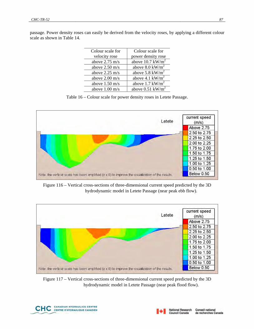
CHC-TR-52 87
passage. Power density roses can easily be derived from the velocity roses, by applying a different colour scale as shown in Table 14.
Colour scale for
velocity rose Colour scale for
power density rose above 2.75 m/s above 10.7 kW/m2 above 2.50 m/s above 8.0 kW/m2 above 2.25 m/s above 5.8 kW/m2 above 2.00 m/s above 4.1 kW/m2 above 1.50 m/s above 1.7 kW/m2 above 1.00 m/s above 0.51 kW/m2
Table 16 – Colour scale for power density roses in Letete Passage.
Figure 116 – Vertical cross-sections of three-dimensional current speed predicted by the 3D
hydrodynamic model in Letete Passage (near peak ebb flow).
Figure 117 – Vertical cross-sections of three-dimensional current speed predicted by the 3D
hydrodynamic model in Letete Passage (near peak flood flow).

CHC-TR-52 88
Figure 118 – Vertical cross-sections of three-dimensional power density predicted by the 3D
hydrodynamic model in Letete Passage (near peak ebb flow).
Figure 119 – Vertical cross-sections of three-dimensional power density predicted by the 3D
hydrodynamic model in Letete Passage (near peak flood flow).
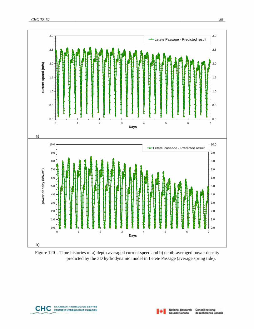
CHC-TR-52 89
0.0
0.5
1.0
1.5
2.0
2.5
3.0
0 1 2 3 4 5 6 7Days
curr
ent s
peed
(m/s
)
0.0
0.5
1.0
1.5
2.0
2.5
3.0Letete Passage - Predicted result
a)
0.0
1.0
2.0
3.0
4.0
5.0
6.0
7.0
8.0
9.0
10.0
0 1 2 3 4 5 6 7Days
pow
er d
ensi
ty (k
W/m
2 )
0.0
1.0
2.0
3.0
4.0
5.0
6.0
7.0
8.0
9.0
10.0Letete Passage - Predicted result
b)
Figure 120 – Time histories of a) depth-averaged current speed and b) depth-averaged power density predicted by the 3D hydrodynamic model in Letete Passage (average spring tide).
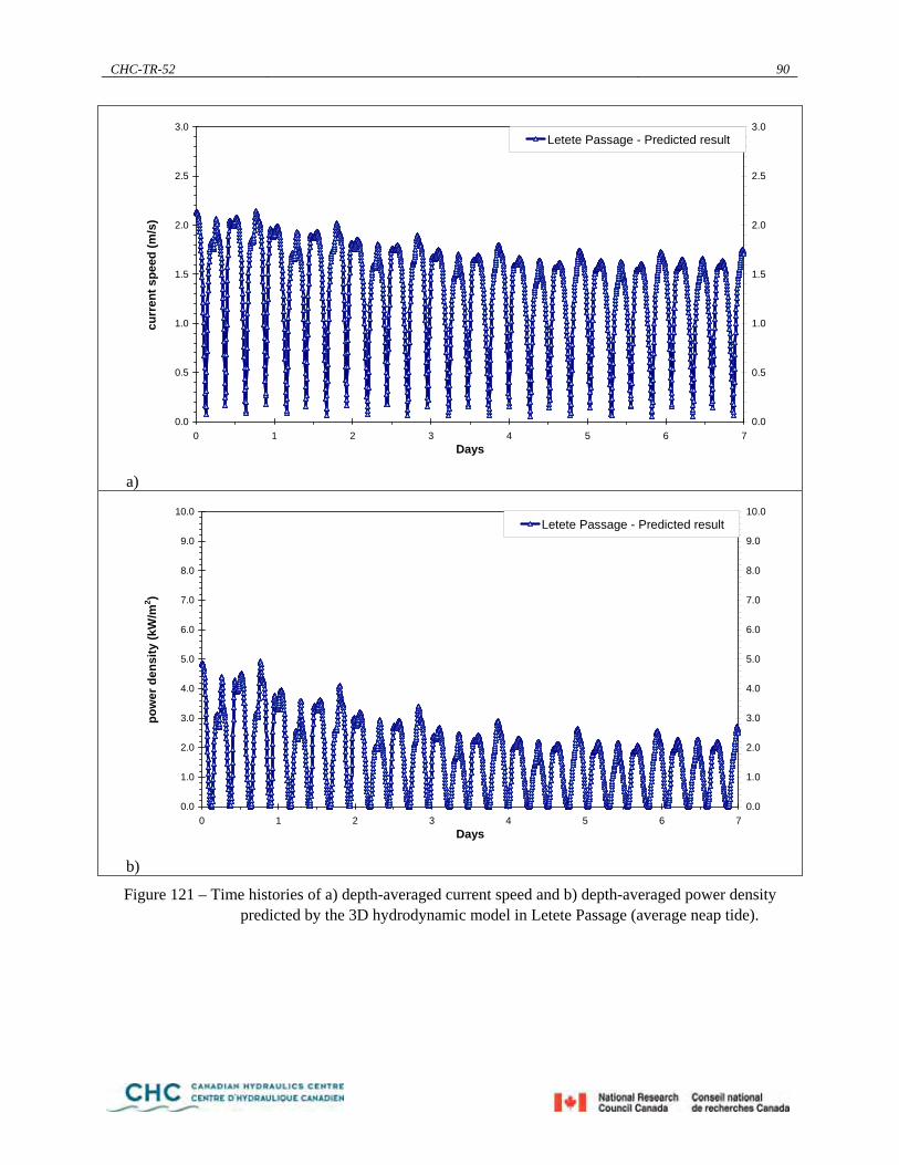
CHC-TR-52 90
0.0
0.5
1.0
1.5
2.0
2.5
3.0
0 1 2 3 4 5 6 7Days
curr
ent s
peed
(m/s
)
0.0
0.5
1.0
1.5
2.0
2.5
3.0Letete Passage - Predicted result
a)
0.0
1.0
2.0
3.0
4.0
5.0
6.0
7.0
8.0
9.0
10.0
0 1 2 3 4 5 6 7Days
pow
er d
ensi
ty (k
W/m
2 )
0.0
1.0
2.0
3.0
4.0
5.0
6.0
7.0
8.0
9.0
10.0Letete Passage - Predicted result
b)
Figure 121 – Time histories of a) depth-averaged current speed and b) depth-averaged power density predicted by the 3D hydrodynamic model in Letete Passage (average neap tide).
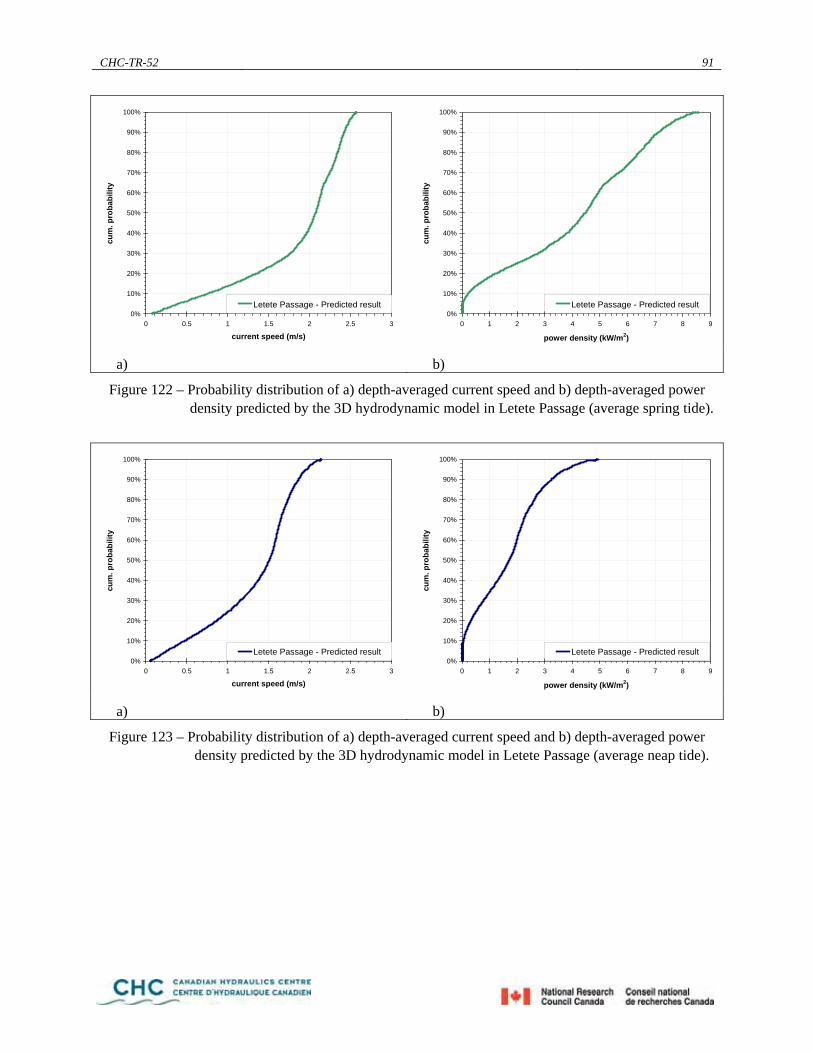
CHC-TR-52 91
0%
10%
20%
30%
40%
50%
60%
70%
80%
90%
100%
0 0.5 1 1.5 2 2.5 3
current speed (m/s)
cum
. pro
babi
lity
Letete Passage - Predicted result
0%
10%
20%
30%
40%
50%
60%
70%
80%
90%
100%
0 1 2 3 4 5 6 7 8 9
power density (kW/m2)
cum
. pro
babi
lity
Letete Passage - Predicted result
a) b)
Figure 122 – Probability distribution of a) depth-averaged current speed and b) depth-averaged power density predicted by the 3D hydrodynamic model in Letete Passage (average spring tide).
0%
10%
20%
30%
40%
50%
60%
70%
80%
90%
100%
0 0.5 1 1.5 2 2.5 3
current speed (m/s)
cum
. pro
babi
lity
Letete Passage - Predicted result
0%
10%
20%
30%
40%
50%
60%
70%
80%
90%
100%
0 1 2 3 4 5 6 7 8 9
power density (kW/m2)
cum
. pro
babi
lity
Letete Passage - Predicted result
a) b)
Figure 123 – Probability distribution of a) depth-averaged current speed and b) depth-averaged power density predicted by the 3D hydrodynamic model in Letete Passage (average neap tide).
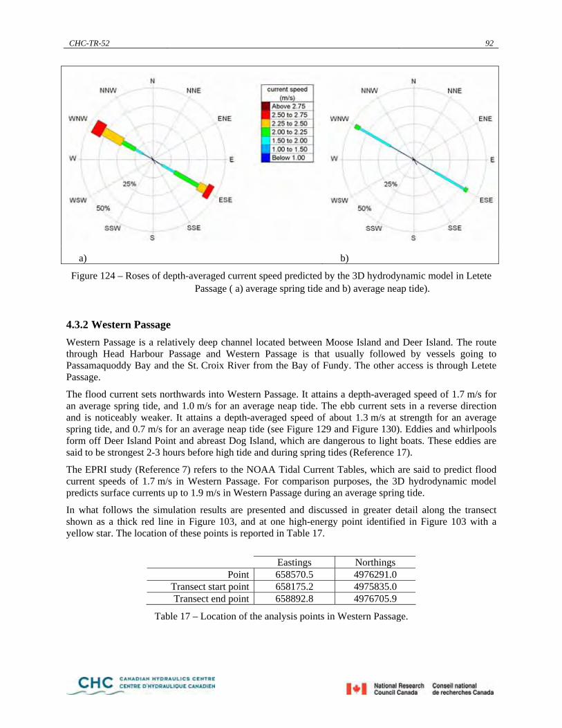
CHC-TR-52 92
a) b)
Figure 124 – Roses of depth-averaged current speed predicted by the 3D hydrodynamic model in Letete Passage ( a) average spring tide and b) average neap tide).
4.3.2 Western Passage Western Passage is a relatively deep channel located between Moose Island and Deer Island. The route through Head Harbour Passage and Western Passage is that usually followed by vessels going to Passamaquoddy Bay and the St. Croix River from the Bay of Fundy. The other access is through Letete Passage.
The flood current sets northwards into Western Passage. It attains a depth-averaged speed of 1.7 m/s for an average spring tide, and 1.0 m/s for an average neap tide. The ebb current sets in a reverse direction and is noticeably weaker. It attains a depth-averaged speed of about 1.3 m/s at strength for an average spring tide, and 0.7 m/s for an average neap tide (see Figure 129 and Figure 130). Eddies and whirlpools form off Deer Island Point and abreast Dog Island, which are dangerous to light boats. These eddies are said to be strongest 2-3 hours before high tide and during spring tides (Reference 17).
The EPRI study (Reference 7) refers to the NOAA Tidal Current Tables, which are said to predict flood current speeds of 1.7 m/s in Western Passage. For comparison purposes, the 3D hydrodynamic model predicts surface currents up to 1.9 m/s in Western Passage during an average spring tide.
In what follows the simulation results are presented and discussed in greater detail along the transect shown as a thick red line in Figure 103, and at one high-energy point identified in Figure 103 with a yellow star. The location of these points is reported in Table 17.
Eastings Northings
Point 658570.5 4976291.0 Transect start point 658175.2 4975835.0 Transect end point 658892.8 4976705.9
Table 17 – Location of the analysis points in Western Passage.

CHC-TR-52 93
Figure 125 to Figure 128 show the variability with location and elevation across Western Passage of the current speed and the kinetic power density at times near peak ebb and peak flood flows. The kinetic power density in Western Passage is predicted to reach 3.7 kW/m2 during peak flood flows. Interestingly, this maximum is predicted to prevail near the bottom of the channel rather than at the surface as one might expect. The corresponding depth-averaged kinetic power density, calculated as the average of the power densities predicted at different elevations in the water column, is 3.4 kW/m2. This estimate is smaller than the peak depth-averaged power density predicted by EPRI and summarised in Table 8.
The mean kinetic power density along the same high-energy transect was also derived from the simulation results by taking the temporal and spatial average of the instantaneous power density. The mean kinetic power density for this transect is predicted to be 0.38 kW/m2. This value can be compared to the EPRI’s estimate of 2.2 kW/m2 for Western Passage (Reference 7 and Table 8).
Time histories of depth-averaged current speed and depth-averaged power density at one high-energy point in Western Passage are displayed in Figure 129 and Figure 130. Cumulative probability distributions were derived from these time histories and are presented in Figure 131 and Figure 132 for average spring and average neap conditions. The median current speed is predicted to vary between 0.7 m/s for average neap tide conditions and 1.0 m/s for average spring tide conditions at this high-energy point. The corresponding median kinetic power densities range between 0.2 kW/m2 and 0.6 kW/m2.
Figure 133 displays the simulation results as velocity roses. The flow is clearly bi-directional at this point in Western Passage. By applying a different colour scale (see Table 12) these velocity density roses can easily be converted to power density roses.
Figure 125 – Vertical cross-sections of three-dimensional current speed predicted by the 3D
hydrodynamic model in Western Passage (near peak ebb flow).
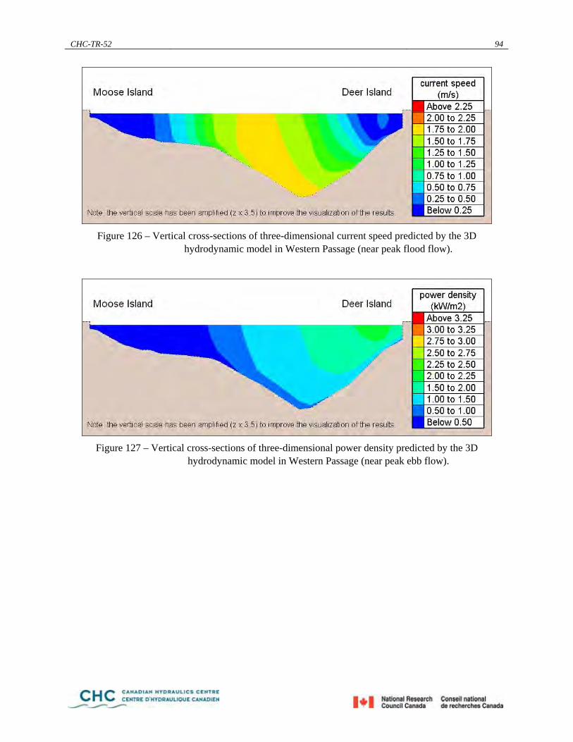
CHC-TR-52 94
Figure 126 – Vertical cross-sections of three-dimensional current speed predicted by the 3D
hydrodynamic model in Western Passage (near peak flood flow).
Figure 127 – Vertical cross-sections of three-dimensional power density predicted by the 3D
hydrodynamic model in Western Passage (near peak ebb flow).

CHC-TR-52 95
Figure 128 – Vertical cross-sections of three-dimensional power density predicted by the 3D
hydrodynamic model in Western Passage (near peak flood flow).

CHC-TR-52 96
0.0
0.2
0.4
0.6
0.8
1.0
1.2
1.4
1.6
1.8
2.0
0 1 2 3 4 5 6 7Days
curr
ent s
peed
(m/s
)
0.0
0.2
0.4
0.6
0.8
1.0
1.2
1.4
1.6
1.8
2.0Western Passage - Predicted result
a)
0.0
0.5
1.0
1.5
2.0
2.5
3.0
3.5
0 1 2 3 4 5 6 7Days
pow
er d
ensi
ty (k
W/m
2 )
0.0
0.5
1.0
1.5
2.0
2.5
3.0
3.5Western Passage - Predicted result
b)
Figure 129 – Time histories of a) depth-averaged current speed and b) depth-averaged power density predicted by the 3D hydrodynamic model in Western Passage (average spring tide).
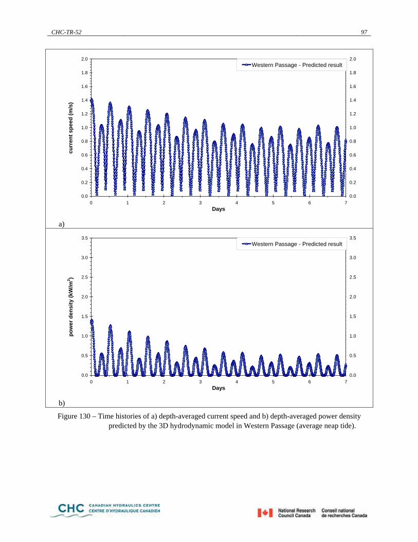
CHC-TR-52 97
0.0
0.2
0.4
0.6
0.8
1.0
1.2
1.4
1.6
1.8
2.0
0 1 2 3 4 5 6 7Days
curr
ent s
peed
(m/s
)
0.0
0.2
0.4
0.6
0.8
1.0
1.2
1.4
1.6
1.8
2.0Western Passage - Predicted result
a)
0.0
0.5
1.0
1.5
2.0
2.5
3.0
3.5
0 1 2 3 4 5 6 7Days
pow
er d
ensi
ty (k
W/m
2 )
0.0
0.5
1.0
1.5
2.0
2.5
3.0
3.5Western Passage - Predicted result
b)
Figure 130 – Time histories of a) depth-averaged current speed and b) depth-averaged power density predicted by the 3D hydrodynamic model in Western Passage (average neap tide).

CHC-TR-52 98
0%
10%
20%
30%
40%
50%
60%
70%
80%
90%
100%
0 0.2 0.4 0.6 0.8 1 1.2 1.4 1.6 1.8
current speed (m/s)
cum
. pro
babi
lity
Western Passage - Predicted result
0%
10%
20%
30%
40%
50%
60%
70%
80%
90%
100%
0 0.5 1 1.5 2 2.5 3
power density (kW/m2)
cum
. pro
babi
lity
Western Passage - Predicted result
a) b)
Figure 131 – Probability distribution of a) depth-averaged current speed and b) depth-averaged power density predicted by the 3D hydrodynamic model in Western Passage (average spring
tide).
0%
10%
20%
30%
40%
50%
60%
70%
80%
90%
100%
0 0.2 0.4 0.6 0.8 1 1.2 1.4 1.6 1.8
current speed (m/s)
cum
. pro
babi
lity
Western Passage - Predicted result
0%
10%
20%
30%
40%
50%
60%
70%
80%
90%
100%
0 0.5 1 1.5 2 2.5 3
power density (kW/m2)
cum
. pro
babi
lity
Western Passage - Predicted result
a) b)
Figure 132 – Probability distribution of a) depth-averaged current speed and b) depth-averaged power density predicted by the 3D hydrodynamic model in Western Passage (average neap tide).

CHC-TR-52 99
a) b)
Figure 133 – Roses of depth-averaged current speed predicted by the 3D hydrodynamic model in Western Passage ( a) average spring tide and b) average neap tide).
4.3.3 Head Harbour Passage Head Harbour Passage is a deep channel, about 6.5 km long, which follows the north-western coast of Campobello Island. North of Campobello Island, the flood sets strongly westward towards Deer Island. Its direction then changes to follow the general orientation of the passage (south-southwesterly) until it reaches Eastport, at which point the flow strongly turns westerly towards Western Passage. The ebb generally sets in a reverse direction.
The simulations indicate that reasonably strong tidal currents occur in Head Harbour Passage. The flood currents are predicted to attain a depth-averaged speed of about 1.1 m/s at strength for an average spring tide, and 0.6 m/s for an average neap tide. The ebb fosters stronger currents with a depth-averaged speed of about 1.4 m/s at strength for an average spring tide, and 0.8 m/s for an average neap tide (see Figure 138 and Figure 139). For reference the United States Coast Pilot (Reference 17) mentions current speeds of 2.6 m/s at times in Head Harbour Passage. These are assumed to be surface currents. The 3D hydrodynamic model predicts surface currents up to approximately 1.6 m/s during an average spring tide. The reasons for this discrepancy require further investigation.
In what follows the simulation results are presented and discussed in greater detail along the transect denoted by a bold red line in Figure 103, and at one high-energy point marked by a yellow star in Figure 103. The location of these points is reported in Table 18.
Eastings Northings
Point 662107.9 4978507.0 Transect start point 662879.1 4978055.1
Transect middle point 661407.2 4978876.9 Transect end point 660352.4 4979330.8
Table 18 – Location of the analysis points in Head Harbour Passage.
CHC-TR-52 100
The variability of the current speed with location and elevation along one transect, at times near peak ebb and peak flood flows, is shown in Figure 134 and Figure 135, while the spatial variability of kinetic power density along this transect for these same times is mapped in Figure 136 and Figure 137. The power density in Head Harbour Passage along this transect is predicted to reach 1.7 kW/m2 during peak ebb flows in the deeper part of the channel, on Campobello Island side. The corresponding depth-averaged kinetic power density, calculated as the average of the power densities predicted at different elevations in the water column, is 1.5 kW/m2. This estimate is substantially smaller than the prediction made by EPRI (see Table 8).
The mean kinetic power density for the same high-energy transect was also computed from the 3D hydrodynamic model simulation results. The mean power density was computed as the spatial and temporal average of the instantaneous power density over the entire transect for the whole (14-day) simulation period representing average tidal conditions. The mean kinetic power density is predicted to be 1.4 kW/m2 in Head Harbour Passage. For comparison purposes, the EPRI study (Reference 7 and Table 8) estimated a value of 1.9 kW/m2, while CHC-TR-41 (Reference 5 and Table 7) reports a value of 1.22 kW/m2 for Head Harbour Passage.
Figure 138 and Figure 139 show time histories of depth-averaged current speed and depth-averaged kinetic power density at one point in Head Harbour Passage. The same results are also presented in terms of cumulative probability distributions in Figure 140 and Figure 141. The median current speed ranges between 0.5 m/s for average neap tide conditions and 0.8 m/s for average spring tide conditions. The corresponding depth-averaged power densities for this point range between 0.1 kW/m2 and 0.3 kW/m2 only.
Figure 142 displays the simulation results at one high-energy point in Head Harbour Passage as velocity roses for 7-day periods comprising an average spring tide and an average neap tide respectively. The location of this point is displayed as a yellow star in Figure 103. By applying a different colour scale, a power density rose can easily be derived from the velocity rose. The correspondence between the two scales is given in Table 10.
Colour scale for
velocity rose Colour scale for
power density rose above 1.50 m/s above 1.7 kW/m2 above 1.25 m/s above 1.0 kW/m2 above 1.00 m/s above 0.5 kW/m2 above 0.75 m/s above 0.2 kW/m2 above 0.50 m/s above 0.1 kW/m2 above 0.25 m/s above 0.01 kW/m2
Table 19 – Colour scale for power density roses in Head Harbour Passage.

CHC-TR-52 101
Figure 134 – Vertical cross-sections of three-dimensional current speed predicted by the 3D
hydrodynamic model in Head Harbour Passage (near peak ebb flow).
Figure 135 – Vertical cross-sections of three-dimensional current speed predicted by the 3D
hydrodynamic model in Head Harbour Passage (near peak flood flow).

CHC-TR-52 102
Figure 136 – Vertical cross-sections of three-dimensional power density predicted by the 3D
hydrodynamic model in Head Harbour Passage (near peak ebb flow).
Figure 137 – Vertical cross-sections of three-dimensional power density predicted by the 3D
hydrodynamic model in Head Harbour Passage (near peak flood flow).
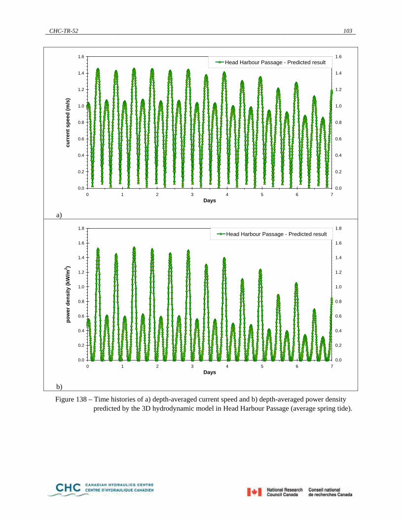
CHC-TR-52 103
0.0
0.2
0.4
0.6
0.8
1.0
1.2
1.4
1.6
0 1 2 3 4 5 6 7Days
curr
ent s
peed
(m/s
)
0.0
0.2
0.4
0.6
0.8
1.0
1.2
1.4
1.6Head Harbour Passage - Predicted result
a)
0.0
0.2
0.4
0.6
0.8
1.0
1.2
1.4
1.6
1.8
0 1 2 3 4 5 6 7Days
pow
er d
ensi
ty (k
W/m
2 )
0.0
0.2
0.4
0.6
0.8
1.0
1.2
1.4
1.6
1.8Head Harbour Passage - Predicted result
b)
Figure 138 – Time histories of a) depth-averaged current speed and b) depth-averaged power density predicted by the 3D hydrodynamic model in Head Harbour Passage (average spring tide).

CHC-TR-52 104
0.0
0.2
0.4
0.6
0.8
1.0
1.2
1.4
1.6
0 1 2 3 4 5 6 7Days
curr
ent s
peed
(m/s
)
0.0
0.2
0.4
0.6
0.8
1.0
1.2
1.4
1.6Head Harbour Passage - Predicted result
a)
0.0
0.2
0.4
0.6
0.8
1.0
1.2
1.4
1.6
1.8
0 1 2 3 4 5 6 7Days
pow
er d
ensi
ty (k
W/m
2 )
0.0
0.2
0.4
0.6
0.8
1.0
1.2
1.4
1.6
1.8Head Harbour Passage - Predicted result
b)
Figure 139 – Time histories of a) depth-averaged current speed and b) depth-averaged power density predicted by the 3D hydrodynamic model in Head Harbour Passage (average neap tide).
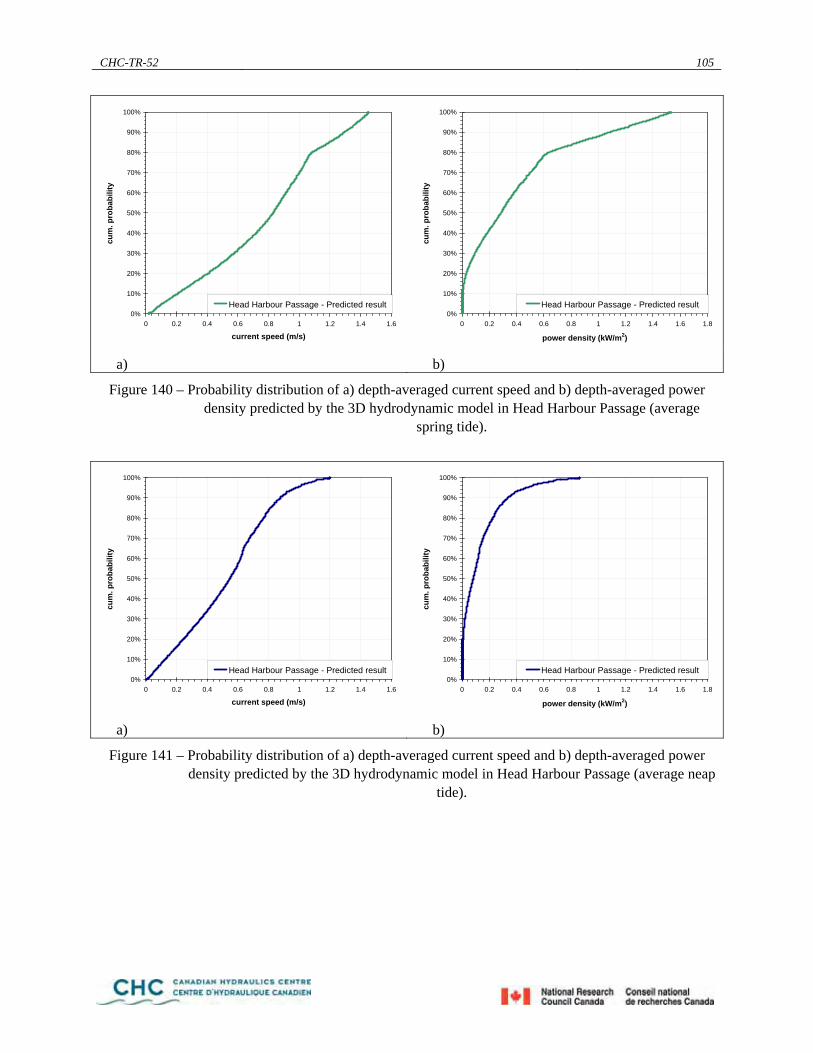
CHC-TR-52 105
0%
10%
20%
30%
40%
50%
60%
70%
80%
90%
100%
0 0.2 0.4 0.6 0.8 1 1.2 1.4 1.6
current speed (m/s)
cum
. pro
babi
lity
Head Harbour Passage - Predicted result
0%
10%
20%
30%
40%
50%
60%
70%
80%
90%
100%
0 0.2 0.4 0.6 0.8 1 1.2 1.4 1.6 1.8
power density (kW/m2)
cum
. pro
babi
lity
Head Harbour Passage - Predicted result
a) b)
Figure 140 – Probability distribution of a) depth-averaged current speed and b) depth-averaged power density predicted by the 3D hydrodynamic model in Head Harbour Passage (average
spring tide).
0%
10%
20%
30%
40%
50%
60%
70%
80%
90%
100%
0 0.2 0.4 0.6 0.8 1 1.2 1.4 1.6
current speed (m/s)
cum
. pro
babi
lity
Head Harbour Passage - Predicted result
0%
10%
20%
30%
40%
50%
60%
70%
80%
90%
100%
0 0.2 0.4 0.6 0.8 1 1.2 1.4 1.6 1.8
power density (kW/m2)
cum
. pro
babi
lity
Head Harbour Passage - Predicted result
a) b)
Figure 141 – Probability distribution of a) depth-averaged current speed and b) depth-averaged power density predicted by the 3D hydrodynamic model in Head Harbour Passage (average neap
tide).

CHC-TR-52 106
a) b)
Figure 142 – Roses of depth-averaged current speed predicted by the 3D hydrodynamic model in Head Harbour Passage ( a) average spring tide and b) average neap tide).

CHC-TR-52 107
5. Conclusions In this study a new numerical hydrodynamic model of the Bay of Fundy was developed to simulate three-dimensional tidal flows and help assess the associated kinetic energy resource in the Bay. The model covers the entire Bay of Fundy and includes a number of tributaries and sub-basins in order to represent, as correctly as possible, the tidal volume variations in the system. The model makes use of the most recent high-resolution bathymetric data collected in the Bay by NRCan.
This new 3D hydrodynamic model was successfully calibrated and validated using information from tide tables published by DFO-CHS, and measurements of water levels and currents archived by DFO-BIO. Overall, the model was demonstrated to provide good predictions of water level fluctuations and currents throughout the Bay of Fundy for both spring and neap tides. It can therefore be applied with confidence to investigate tidal currents in the Bay. The model’s predictions will, however, be most accurate in areas where good bathymetric information was available and a fine mesh has been used. This includes most of the high-energy areas of special interest identified in previous studies. It is important to recognize that tidal current predictions for certain other areas may be less reliable.
The new 3D hydrodynamic model was applied to simulate tidal flows over a 15-day period featuring average spring and average neap tides. Simulation results for this period can be considered to be representative of conditions over longer durations. Simulation results for seven key areas have been presented and discussed in detail. These areas are Minas Passage, Petit Passage, Grand Passage, and Digby Gut in Nova Scotia and Western Passage, Head Harbour Passage, and Letete Passage in New Brunswick. The results presented herein provide a detailed description of the scale and many attributes of the kinetic energy resources in each of these areas.
Tidal current resources are best characterized by the mean power, which represents an integration or averaging of temporal fluctuations over time. The mean power density characterizes the average intensity of the flow at the site. Energy extraction will not be feasible if the flows are too weak for efficient operation of an energy conversion device. On the other hand, safe installation, operation and maintenance could also be difficult if the flows are excessively strong.
The mean kinetic power density has been calculated for a single transect in each key area. The estimates have been obtained by integrating the depth-averaged power density multiplied by the depth along each of the transects and dividing by the corresponding cross-sectional area. This analysis yielded a time history of power density representative of the whole transect. The average power density for each transect was calculated and is reported in Table 20 for average spring conditions, for average neap conditions and for an average 14-day spring-neap cycle. These estimates can be compared to those derived by EPRI from their analysis of data from published sources such as nautical charts, current tables and sailing directions combined with engineering assumptions (Reference 7 and Reference 8), and to those reported in CHC-TR-41 (Reference 5). Examination of Table 20 reveals some significant differences between the mean power densities predicted by the two previous studies, and between the previous predictions and the estimates derived in this study from analysis of the new 3D simulation results. New velocity measurements in critical areas will go a long way towards resolving these differences. Overall, the depth-averaged mean power densities predicted by the new hydrodynamic model are in closer agreement with the values reported in Reference 5.
The full three-dimensional simulation results can be accessed through a computer application named MarKE-Fundy3D that has been developed as part of this study. While providing a diverse community of interested stakeholders with direct and easy access to detailed information on tidal currents and kinetic energy resources throughout the Bay, MarKE-Fundy3D also provides users with the ability to forecast the power production from hypothetical energy conversion devices installed at any location and elevation within the water column. MarKE-Fundy3D can be used to obtain a detailed understanding of the resource,

CHC-TR-52 108
including its temporal and spatial attributes, and to conduct “what-if” evaluations of alternative sites. The new 3D hydrodynamic model and the MarKE-Fundy3D application can be used to greatly enhance the preliminary assessment of potential sites, but are not intended to replace the need for detailed site investigations to support specific developments, such as the Fundy Tidal Institute.
The physical and ecological impacts of removing energy from natural tidal flows must be carefully assessed before reliable predictions can be made concerning the size of the extractable kinetic energy resource at any site. Good information on the physical and ecological impacts of removing various amounts of energy from particular locations must be developed before such an assessment can be made.
The new three-dimensional hydrodynamic model developed and calibrated during this study can now be applied to simulate the effects of removing various amounts of energy from different locations throughout the Bay. The new model can be applied to obtain reliable predictions of the potential changes in water levels and flow velocities due to various hypothetical energy removal scenarios. For example, the model can be applied to simulate and assess the physical impacts of extracting 1 MW, 10 MW, and 100 MW of energy from Minas Passage. The ability of the TELEMAC system to perform this type of simulation has already been demonstrated at a high-energy site on the St. Lawrence River near the City of Cornwall, Ontario (see Reference 2). Such studies are urgently required in order to help establish a rational scientific basis for determining what fraction of the available kinetic energy resource can be safely extracted from any given area.
Depth-averaged mean power density
Location average spring tide
average neap tide
average 14-day cycle
(source: EPRI)
(source: CHC-TR-41)
NEW BRUNSWICK
Western Passage 0.57 kW/m2 0.19 kW/m2 0.38 kW/m2 2.2 kW/m2 - Head Harbour Passage 0.26 kW/m2 0.09 kW/m2 0.18 kW/m2 1.9 kW/m2 1.22 kW/m2
Letete Passage 2.0 kW/m2 0.79 kW/m2 1.4 kW/m2 3.7 kW/m2 1.22 kW/m2
NOVA SCOTIA Petit Passage 4.9 kW/m2 2.7 kW/m2 3.8 kW/m2 7.7 kW/m2 3.35 kW/m2
Grand Passage 0.60 kW/m2 0.31 kW/m2 0.47 kW/m2 4.9 kW/m2 2.11 kW/m2 Digby Gut 1.4 kW/m2 0.51 kW/m2 0.94 kW/m2 1.8 kW/m2 1.22 kW/m2
Minas Passage 9.1 kW/m2 4.3 kW/m2 6.7 kW/m2 4.9 kW/m2 6.04 kW/m2 2
Table 20 – Summary of predicted mean kinetic power densities at potential sites in New Brunswick and Nova Scotia.
2 Minas Basin.

CHC-TR-52 109
6. Acknowledgement This report was funded by the Technology and Innovation Program, Office of Energy Research and Development, Natural Resources Canada, in partnership with the Department of Energy, Province of New Brunswick, and the Department of Energy, Province of Nova Scotia.
7. References Reference 1 Cornett, A., Zhang, J. “Near-shore Wave Climate and Wave Energy Resources, Western
Vancouver Island, B.C.”, NRC Canadian Hydraulics Centre Technical Report CHC-TR-51. Ottawa, 2008.
Reference 2 Faure, T., Cornett, A. “St. Lawrence River Currents – A Source of Renewable Kinetic Energy.” NRC Canadian Hydraulics Centre Technical Report CHC-TR-53. Ottawa, 2008.
Reference 3 E.D.F.-D.E.R., “TELEMAC-3D, Version 2.2 – Note de principe”, 1997.
Reference 4 E.D.F.-D.E.R., “TELEMAC-3D, Version 2.1 – Validation document”, 1997.
Reference 5 Cornett, A. “Inventory of Canada’s Marine Renewable Energy Resources”, National Research Council Canadian Hydraulics Centre, Technical Report No. CHC-TR-041, 2006.
Reference 6 “Maine Tidal In-Stream Energy Conversion (TISEC): Survey and Characterization of Potential Project Sites.” Electric Power Research Institute, Report No. EPRI-TP-003-ME Rev1, October 2006.
Reference 7 “New Brunswick Tidal In-Stream Energy Conversion (TISEC): Survey and Characterization of Potential Project Sites.”Electric Power Research Institute, Report No. EPRI-TP-003-NB Rev1, October 2006.
Reference 8 “Nova Scotia Tidal In-Stream Energy Conversion (TISEC): Survey and Characterization of Potential Project Sites.” Electric Power Research Institute, Report No. EPRI-TP-003-NS Rev2, October 2006.
Reference 9 Colour satellite images captured from Google maps (http://www.maps.google.com)
Reference 10 Bathymetry of the Gulf of Maine downloaded from the Massachusetts Geographic Information System website (http://www.mass.gov/mgis/bathymgm.htm).
Reference 11 WebTide Tidal Prediction Model, Fisheries and Oceans Canada. (http://www.mar.dfo-mpo.gc.ca/science/ocean/coastal_hydrodynamics/WebTide/webtide.html).
Reference 12 Observed water level data downloaded from the DFO Integrated Science Data Management website (http://www.meds-sdmm.dfo-mpo.gc.ca/meds/Databases/TWL/TWL_e.htm).
Reference 13 “Canadian Tide and Current Tables, Volume 1, Atlantic Coast and Bay of Fundy.” Fisheries and Oceans Canada Canadian Hydrographic Services, 2007 (http://www.tides.gc.ca).
Reference 14 Garrett, C., Cummins, P. “Generating Power from Tidal Currents.” J. Waterway , Port, Coastal and Ocean Eng. 130, pp 114-118, 2004.

CHC-TR-52 110
Reference 15 Bryden, I., Grinsted, T., Melville, G. “Assessing the Potential of a Simple Channel to Deliver Useful Energy.” J. Applied Ocean Research. 26 pp 198-204, 2004.
Reference 16 “Atlas of Tidal Currents, Bay of Fundy and Gulf of Maine.” Fisheries and Oceans Canada Canadian Hydrographic Services, 1981.
Reference 17 “United States Coast Pilot 1 - 37th edition.” U.S. Department of Commerce, National Oceanic and Atmospheric Administration, 2007.


