Embed Size (px)
Citation preview

HAL Id: hal-00750978https://hal.inria.fr/hal-00750978
Submitted on 12 Nov 2012
HAL is a multi-disciplinary open accessarchive for the deposit and dissemination of sci-entific research documents, whether they are pub-lished or not. The documents may come fromteaching and research institutions in France orabroad, or from public or private research centers.
L’archive ouverte pluridisciplinaire HAL, estdestinée au dépôt et à la diffusion de documentsscientifiques de niveau recherche, publiés ou non,émanant des établissements d’enseignement et derecherche français ou étrangers, des laboratoirespublics ou privés.
3D model based tracking for omnidirectional vision: anew spherical approach.
Guillaume Caron, El Mustapha Mouaddib, Eric Marchand
To cite this version:Guillaume Caron, El Mustapha Mouaddib, Eric Marchand. 3D model based tracking for omnidirec-tional vision: a new spherical approach.. Robotics and Autonomous Systems, Elsevier, 2012, 60 (8),pp.1056-1068. <10.1016/j.robot.2012.05.009>. <hal-00750978>

3D model based tracking for omnidirectional vision:
a new spherical approach
Guillaume Caron1, El Mustapha Mouaddib1 and Eric Marchand2
1Universite de Picardie Jules Verne, MIS laboratory, Amiens, France{guillaume.caron, mouaddib}@u-picardie.fr
2Universite de Rennes 1, IRISA/INRIA Lagadic, Rennes, [email protected]
Abstract
The current work addresses the problem of 3D model tracking in thecontext of monocular and stereo omnidirectional vision in order to estimatethe camera pose. To this end, we track 3D objects modeled by line segmentsbecause the straight line feature is often used to model the environment.Indeed, we are interested in mobile robot navigation using omnidirectionalvision in structured environments. In the case of omnidirectional vision,3D straight lines are projected as conics in omnidirectional images. Undercertain conditions, these conics may have singularities.
In this paper, we present two contributions. We, first, propose a newspherical formulation of the pose estimation withdrawing singularities, us-ing an object model composed of lines. The theoretical formulation and thevalidation on synthetic images show thus the new formulation clearly outper-forms the former image plane one. The second contribution is the extensionof the spherical representation to the stereovision case. We consider in thepaper a sensor which combines a camera and four mirrors. Results in varioussituations show the robustness to illumination changes and local mistrack-ing. As a final result, the proposed new stereo spherical formulation allows tolocalize online a robot indoor and outdoor whereas the classical formulationfails.
Keywords:Omnidirectional vision, stereovision, spherical optimization, tracking
Preprint submitted to Robotics and Autonomous Systems March 21, 2012
1. Introduction
Pose estimation can be done using image features, i.e. points, lines, orother geometrical features. When considering the availability of a partial3D model of an object or a scene, these features need to be extracted fromimages and associated to the 3D model. This association process is generallydone in a first image and features are then tracked over time, while the objectand/or the camera is moving.
When using a perspective camera, the spatial volume in which the objectcan be moved, and still be perceived by the camera, is limited. Hence,objects can appear partially in images. This is particularly the case whenthe camera is moving within an environment of which a 3D model, evenpartial, is tracked.
Omnidirectional cameras, thanks to their very wide field of view, allowto track image features during a long period of time, when moving. Thisis synonym of efficiency, precision and robustness for the tracking and poseestimation processes. Using such a camera allows to keep the object in theimage even if it moves in a wide spatial volume surrounding the camera.
A complementary way to increase robustness in a tracking and pose es-timation process is to add perception redundancy using several cameras ac-quiring synchronously images of the object. An interesting idea is thus touse a vision sensor merging stereovision and omnidirectional vision. Differentomnidirectional stereovision sensors were designed [1, 2, 3, 4]. We propose touse the Four On One sensor (FOO), a catadioptric sensor made of a uniquecamera and four parabolic mirrors placed in a square at an equal distancefrom the camera [5, 6] (Fig. 1).
The pose estimation problem using 2D-3D correspondences can be tack-led by linear formulations for various features: points [7, 8, 9], lines [10, 11],etc. A problem raised by these formulations is to deal with outliers. Theyappear in presence of partial occlusions or specular reflections. RANSAC [12]techniques allow to reject outliers in an iterative procedure. Although effi-cient to reject outliers it is not really well suited to handle noise in imagemeasurements. Recent works affect a weight to image measurements in lin-ear methods to solve this issue [13, 14]. However, these methods currentlydo not deal with outliers as efficiently as non-linear optimization methods tocompute the pose.
The non-linear formulation of the pose computation issue leads to theusual optimization methods such as steepest descent, Gauss-Newton or
2

Levenberg-Marquardt. These methods consider first order derivatives of acost function formalizing the error in the image between the observation andthe projection of some model for a given pose. The main idea is to alignthe forward projection of the model to image measurements. Some morerecent works use derivatives of the non-linear function of a higher order [15].Several works about non-linear pose computation has been proposed in theoptimization community [16, 17, 18]. As well as in the perspective visioncommunity, many works exist [19, 20, 21], where the main differences rely onthe rotation parameterization (Euler angles, quaternion, vector-angle). Rea-soning on the velocities of camera pose elements, the virtual visual servoing(VVS) [22, 23], is a full scale non-linear optimization technique which can beused for pose computation [24].
Some works have been done about 3D model based tracking and poseestimation using VVS, for perspective camera [24], stereo perspective rig [25]and even for monocular omnidirectional vision [26, 27]. These works also dealwith corrupted data, which is frequent in image feature extraction, using thewidely accepted statistical techniques of robust M-estimation [28], giving aweight, dynamically computed, that reflects the confidence we have in eachmeasure [24, 27, 29].
As we are interested by indoor and outdoor mobile robot navigation, wechoose to consider straight lines as features because they are frequent (doors,corridors, ...) and an omnidirectional vision sensor to recover the robot pose.The main problem in the case of omnidirectional vision, is that 3D straightlines are projected as conics in the omnidirectional image. This propertyinduces two issues: the conics extraction, which is not easy in noisy images,and the conics representation, which has a singularity when the 3D lines arein the same plane as the optical axis.
In this paper, we present two contributions. We, first, propose a newspherical formulation of the pose estimation by VVS, using an object modelcomposed of lines, withdrawing singularities. The second contribution is anextension of this scheme to an omnidirectional stereovision sensor, which ismade with four mirrors and a single camera.
The paper is organized as follows. First, the sensors used in experimentsare described and their projection models recalled in section 2. Then the newformulation of this feature and its consequences are presented in section 3.Both formulations are fairly compared on synthetical images (section 3.7).The extension to stereoscopic systems is finally presented and results on realimages show the achievement of the proposed approach in section 4. Several
3

problematic cases are studied and they highlight the superiority of the newformulation for omnidirectional vision and stereovision, particularly in poseestimation experiment of a mobile robot. A discussion in section 5 analyzes,sums up the contributions of the paper and concludes on perspectives of thework.
2. Sensors and models
In this work, an orthographic camera combined with a paraboloidal mir-ror, in the monocular case, and with several paraboloidal mirrors, in thestereo case, are considered. This configuration has single viewpoint propertyand is also called a central camera [30].
2.1. Unified central projection model
We propose to use the unified projection model for central cameras [31].According to this model, a single viewpoint projection can be modeled by astereographic projection involving a unitary sphere. This is equivalent to adhoc models of central cameras but has the advantage to be valid for a set ofdifferent cameras [32]. Hence, a 3D point X = (X, Y, Z)T is first projected onthis unitary sphere as XS , thanks to the spherical projection function prS(.):
XS =
XSYSZS
= prS(X) with
XS = X
ρ
YS = Yρ
ZS = Zρ
(1)
where ρ =√X2 + Y 2 + Z2. Then, XS is projected in the normalized image
plane as x by a perspective projection, i.e. x = pr(XS), thanks to a secondprojection center for which the sphere has coordinates (0, 0, ξ)T. The directrelationship between X and x defines the projection function prξ:
x = prξ(X) with
{x = X
Z+ξρ
y = YZ+ξρ
(2)
x is a point of the normalized image plane and is transformed in pixeliccoordinates u thanks to the intrinsic matrix K: u = Kprξ(X) = prγ(X),where γ = {αu, αv, u0, v0, ξ} is the set of intrinsic parameters.
4
The projection from the sphere to the image plane is invertible, allowingto retrieve a spherical point from an image point:
XS = pr−1ξ (x) =
ξ+√
1+(1−ξ2)(x2+y2)x2+y2+1
x
ξ+√
1+(1−ξ2)(x2+y2)x2+y2+1
y
ξ+√
1+(1−ξ2)(x2+y2)x2+y2+1
− ξ
(3)
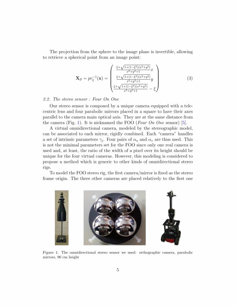
2.2. The stereo sensor : Four On One
Our stereo sensor is composed by a unique camera equipped with a tele-centric lens and four parabolic mirrors placed in a square to have their axesparallel to the camera main optical axis. They are at the same distance fromthe camera (Fig. 1). It is nicknamed the FOO (Four On One sensor) [5].
A virtual omnidirectional camera, modeled by the stereographic model,can be associated to each mirror, rigidly combined. Each “camera” handlesa set of intrinsic parameters γj. Four pairs of αu and αv are thus used. Thisis not the minimal parameters set for the FOO since only one real camera isused and, at least, the ratio of the width of a pixel over its height should beunique for the four virtual cameras. However, this modeling is considered topropose a method which is generic to other kinds of omnidirectional stereorigs.
To model the FOO stereo rig, the first camera/mirror is fixed as the stereoframe origin. The three other cameras are placed relatively to the first one
Figure 1: The omnidirectional stereo sensor we used: orthographic camera, parabolicmirrors, 90 cm height
5

and their relative poses to the first camera are noted as homogeneous matricesc2Mc1 ,
c3Mc1 and c4Mc1 . These poses and the four intrinsic parameters setsmodel the full stereo system. One can note this model is expendable to morecameras/mirrors, knowing each γj and cjMc1 .
3. Model based tracking on theequivalent sphere
The pose estimation method optimizes the pose of the camera relativelyto an object, minimizing the error between the forward projection of theobject 3D model and image measurements (Fig. 2).
In this work, we consider that indoor and urban outdoor environments aremade of 3D segments. Figure 3 details the model of a 3D line, its projectionon the equivalence sphere as a portion of great circle (intersection betweenP1 and S) and then its projection on image place, as a conic. In our previouswork [34], we minimized the point-to-conic distance in the omnidirectionalimage plane. The error is computed between the latter conic and samplepoints like in [27]. The main drawback of this approach is the degeneracyof the conic when its 3D line forms a plane with the optical axis of thecamera [31]. These lines project as radial straight lines in omnidirectionalimages. A solution could be to combine two representations, the conic andthe line in the image, but the problem is still present when a 3D straightline is near the singular case. Indeed, in that case, the conic is very badconditioned, leading to perturbations in the computation of the distance(algebraic measure), between a point and the conic.
Figure 2: Looking for the corresponding edge along normal vectors (blue) to the conic(green) in each sample (red) of the projected 3D model using the moving edge method [33].
6

Figure 3: Projection of a 3D straight line, defined by the intersection of planes P1 and P2,as a great circle on the sphere S.
Finally, computing a geometric distance between a point and the pro-jection of a 3D straight line, rather than an algebraic one, is more efficientwhen the conic is badly conditioned and is more discriminant since it is atrue distance [35].
To solve these issues, we propose to reformulate the point-to-line featureon the sphere of the unified projection model. This solves the first singularityproblem of the projection of a 3D line as a conic. Indeed, even if a 3Dstraight line forms a plane with the camera axis, its projection on the sphereis not singular. Furthermore, minimizing the point-to-line distance on theequivalent sphere, which is now a point-to-great circle distance, rather than inthe image plane allows to easily use a geometric distance as feature, contraryto the conic case.
3.1. Algorithm overview
The goal of the proposed algorithm is to track a known moving object ina sequence of images. As in almost all tracking algorithm, we assume thatthe motion of the object between two images is small. Image measurementsare first of all taken and are the input of the following tracking and poseestimation procedure:
1. Consider an initial pose cMo of the object, usually the optimal pose of
7

the previous image (manual selection for the first image of the sequence,in experiments of this paper).
2. Project the 3D model on the sphere and sample it. A set of points isthus generated for each segment of the 3D model.
3. Project these points in the current image for pose cMo. They may notfit to the actual object (Fig. 2) since it moved between the two images.
4. Apply the moving edge algorithm [33] to each conic of the 3D modelin the image to find the set of sample points on the real correspondingcontour.
5. Back-project the obtained points on the sphere.
6. Compute the point-to-great circle distances and interaction matrices.
7. Apply the VVS control law to compute the update vector of the pose.
Both latter items are repeated until convergence. Then, the next image ofthe sequence is waited and the process restart at the first item of the list.
Following sections are organized as follows. First, the spherical virtualvisual servoing is presented (section 3.2) as it introduces what need to becomputed to optimize the pose. Then the new point-to-great circle featureis defined in section 3.3 as well as a way to process the image to extractmeasurements (section 3.4), its Jacobian (sections 3.5 and 3.6), needed forthe VVS. Figure 4 graphically sums up the algorithm before tackling itsvalidation on synthetic data in section 3.7.
3D space sphere image plane
3D line great circle
ini1al points
ini1al points image
contour points
contour points
image Jacobian
camera veloci1es
control law
prS pr
pr!!1
moving edge
sampling
distances
Figure 4: Synopsis of the algorithm.
8

3.2. Virtual visual servoing
3.2.1. General formulation
The virtual spherical camera is defined by its projection function prS(.)and the 3D object by several features oS defined in its own frame. The VVSmethod estimates the real pose cMo of the object in the camera frame byminimizing the error ∆ (eq. (4)). ∆ is computed between the set of detectedspherical features s∗ and the position s(r) of the same features computed byforward projection. r = [tX , tY , tZ , θuX , θuY , θuZ ] is a vector representationof the pose cMo (3 translation and 3 rotation parameters). Considering kfeatures, ∆ is defined as:
∆ =k∑i=1
(si(r)− s∗i )2, with s(r) = prS(cMo,
oSi). (4)
i indexes the i-th feature of the set.With this formulation, a virtual spherical camera, with initial pose cM0
o,is moved using a visual servoing control law to minimize the error ∆. Atconvergence, the virtual sphere reaches the pose cM∗
o which minimizes ∆.Assuming this non-linear estimation process converges, this pose is the realpose. To sum up, this positioning task is expressed as the regulation of theerror
e = s(r)− s∗. (5)
Imposing an exponential decoupled decrease of the error, e = −λe leadsto the optimization of the pose so that the error evolution curve has anexponential decreasing profile. e depends on s. The image features motionis linked to the virtual camera velocity v [36]:
s = Lsv. (6)
v = (υ, ω)T is the velocity vector of the pose with υ = (υX , υY , υZ), the trans-lation velocity and ω = (ωX , ωY , ωZ), the rotation velocity. Ls is the inter-action matrix (or image Jacobian) linking the features motion to the cameravelocity.
3.2.2. Robust formulation
To make the pose estimation more robust, it has to deal with outliers andthe use of M-estimator [28] is an efficient solution in this way. Some func-tions exist in the literature and apply well to our problem [37]. They allow
9

uncertain measures to be less likely considered and in some cases completelyrejected. To add robust estimation to our objective function ∆ (eq. (4)), itis modified as:
∆R =k∑i=1
P(si(r)− s∗i ), (7)
where P(a) is a robust function that grows subquadratically and is monoton-ically non-decreasing with increasing |a|. For P, we considered the Tukey’sfunction [28] because it completely rejects outliers and give them a zeroweight. This is of interest in virtual visual servoing so that detected outliershave no effect on the virtual camera motion [38].
Iterative Re-Weighted Least Squares is a common method of applyingthe M-estimator. Thus, the error to be regulated to 0 is redefined, takingthe robust function into account:
e = D(s(r)− s∗), (8)
where D is a diagonal weighting matrix given by D = diag(w1, ..., wk). Eachwi is a weight given to specify the confidence in each feature location and iscomputed using statistics on the error vector [24].
A simple control law that allows to move the virtual camera can be de-signed to try to ensure an exponential decoupled decrease of e:
v = −λ (DLs)+D (s(r)− s∗) . (9)
where λ is a gain that tunes the convergence rate and the matricial operator( )+ denotes the left pseudo inverse of the matrix inside the parentheses.
The pose cMo is then updated using the exponential map e[.] of SE(3) [39]:
cMt+1o = cMt
oe[v], (10)
The feature type choice and hence the interaction matrix expression area key point of this algorithm. As previously mentioned, we chose the poin-to-great circle feature and next sections describe the spherical virtual visualservoing for it.
3.3. Definition of the point-to-great circle feature
As we can see in figure (3), the 3D line can be represented by the inter-section of two planes. These two planes P1 and P2 are defined, in the sphereframe, by:
P1 : A1X +B1Y + C1Z = 0
P2 : A2X +B2Y + C2Z +D2 = 0(11)
10
with the following constraints on the 3D parameters:A2
1 +B21 + C2
1 = 1
A22 +B2
2 + C22 = 1
A1A2 +B1B2 + C1C2 = 0
(12)
so that the two planes are orthogonal with unit normals N1 = (A1, B1, C1)T
and N2 = (A2, B2, C2)T. D2 is the orthogonal distance of the 3D line to the
unified model sphere origin.The spherical projection of a 3D line is then defined as the intersection
of the unitary sphere S and plane P1:{X2 + Y 2 + Z2 = 1
A1X +B1Y + C1Z = 0. (13)
Since features are lying on the sphere surface, the normal vector N1 is suffi-cient to parameterize the great circle.
Considering a point XS on the sphere, i.e. an image contour point pro-jected on the sphere, its signed distance to the great circle is expressed bythe dot product d = N1.XS :
d = A1XS +B1YS + C1ZS (14)
This signed distance is interesting since d = 0 when the point is on the greatcircle and tends to ±1 when going away the great circle.
The interaction matrix linked to this distance is expressed consideringthe time variation of d, with XS constant during the pose optimization ofone image :
d = A1XS + B1YS + C1ZS . (15)
This clearly depends on the interaction matrix of N1, i.e. its variation withrespect to the pose. It is described in the following section.
3.4. Measuring edge image points
We mention that edge image points are measured since they are obtainedthanks to initial points computed from the 3D model projection at an initialpose. This is the low level tracking method already used in [33]. Let us notethat it is different to a point detection method.
11

Points used to compute the point-to-great circle distance are obtainedthanks to an adaptation of the moving edge method to omnidirectional im-ages [34]. In the latter work, a 3D segment of the 3D model is projected as aconic in the omnidirectional image. The method needs a regular sampling ofthe conic in order to use the obtained sample points as initial positions forthe edge searching, along normal directions to the conic. However, a conic tocircle transformation and its inverse are necessary for the regular sampling.Indeed, the direct regular sampling of the conic is not trivial, but for a circle,it is.
In the current work, as introduced in the algorithm overview (section 3.1),the sampling of the 3D line projection is done on its corresponding portionof great circle, i.e. on the sphere. It allows a direct regular sampling, con-trary to the conic case. Samples are then projected in the image to find thecorresponding contour thanks to the moving edge method.
3.5. Interaction matrix for the great circle
The interaction between the time variation of the normal vector to thegreat circle and the camera motion is expressed from N1 = (A1, B1, C1)
T [40]:
N1 = − 1
D2
N1NT2 υ −N1 × ω, (16)
with υ and ω, the translation and rotation velocities of the spherical camera(section 3.2.1). The time variation of N1 leads to the interaction matrixlinked to the projection of a 3D line on the sphere:
LN1 =
LA1
LB1
LC1
=
[− 1
D2
N2NT1 [N1]×
](17)
3.6. Interaction matrix for the point-to-great circle distance feature
From equation (15), and knowing the elements of LN1 (eq. (17)), theinteraction matrix Ld related to the point-to-great circle distance is expressedas:
Ld =
XSYSZS
TLA1
LB1
LC1
. (18)
The feature of the VVS is the signed distance d (eq. (14)). So, consideringk features, as in equation (7), the stacking of the k point-to-line distances
12

for current pose gives s(r). The goal of the optimization is to reach nulldistances between points to great circle and hence, s∗ = 0 (a k-vector withall elements equal to zero). Finally, the stacking of the k interaction matricesLd leads to Ls and equation (8) allows to compute the update vector of thepose.
3.7. Validation on synthetic images
This section presents results obtained on images synthesized using thePov-Ray software. The goal of these experiments is to study the behaviorand accuracy of our proposed approach (S) comparing to the image planebased (IP) [27], and their impact on the estimated pose. The implementationhas been done in C++ using the ViSP library [41].
To do this evaluation, two kinds of omnidirectional images are processed.One kind presents a box where lines are not radial in the image (Fig. 5) andthe other presents a majority of radials (Fig. 6). The latter case is a near-singular situation for the image plane (IP) formulation in which it should beless efficient than in the former case, and also less efficient than the sphericalformulation (S).
The experiments done with synthetical images allow to evaluate the con-vergence rate of the algorithms and their robustness to noise in the previ-ously mentioned situations. The pose estimation error at convergence andthe conditioning of interaction matrices are good tools to better understandthe behavior of algorithms.
Three sets of experiments are led to evaluate the:
1. robustness to initialization: several different initial poses with a uniquedesired pose (robust estimation or not) (128 different initial poses).Random variations of the optimal pose are computed in order to benot too far in images for the low level moving edge to succeed.
2. robustness to low quality camera parameters: different level of noise(1 %, 2.5 %, 5 %) applied to the camera intrinsic parameters in termsof percentage of parameter values (1000 random choices each)
3. robustness to low quality 3D model of the object (i.e. the model is notexactly the same as the real object, due to fabrication or measurementerrors of the object): different level of noise (1 %, 2.5 %, 5 %) appliedto the vertices of the object 3D model (1000 random choices each)
The two latter sets of experiments are led considering the robust estimation.For experiments with noisy camera parameters or 3D model vertices, the
13
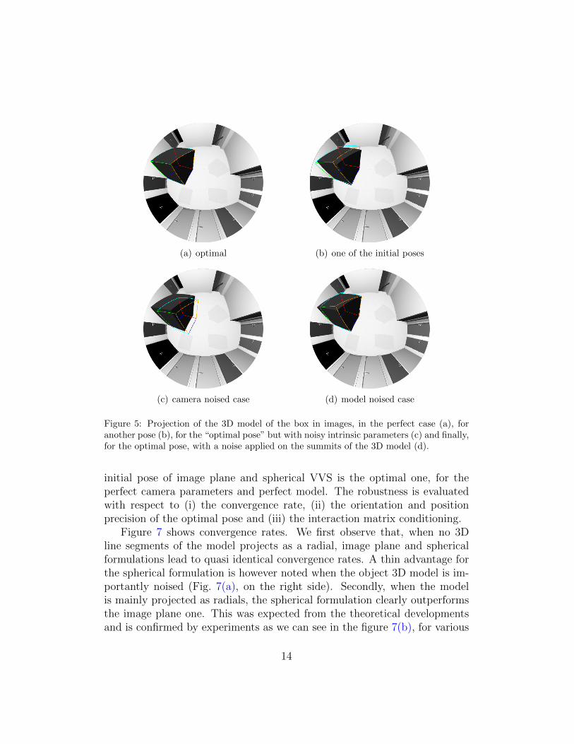
(a) optimal (b) one of the initial poses
(c) camera noised case (d) model noised case
Figure 5: Projection of the 3D model of the box in images, in the perfect case (a), foranother pose (b), for the “optimal pose” but with noisy intrinsic parameters (c) and finally,for the optimal pose, with a noise applied on the summits of the 3D model (d).
initial pose of image plane and spherical VVS is the optimal one, for theperfect camera parameters and perfect model. The robustness is evaluatedwith respect to (i) the convergence rate, (ii) the orientation and positionprecision of the optimal pose and (iii) the interaction matrix conditioning.
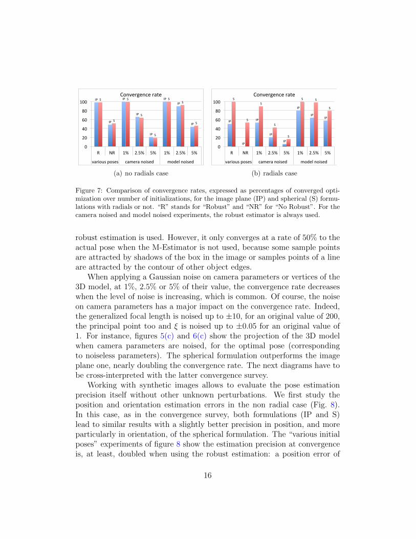
Figure 7 shows convergence rates. We first observe that, when no 3Dline segments of the model projects as a radial, image plane and sphericalformulations lead to quasi identical convergence rates. A thin advantage forthe spherical formulation is however noted when the object 3D model is im-portantly noised (Fig. 7(a), on the right side). Secondly, when the modelis mainly projected as radials, the spherical formulation clearly outperformsthe image plane one. This was expected from the theoretical developmentsand is confirmed by experiments as we can see in the figure 7(b), for various
14

(a) optimal (b) one of the initial poses
(c) camera noised case (d) model noised case
Figure 6: Same different cases than in figure 5 but the pose is such that the box edges aremainly projected as radials in the image.
initial poses with or without robust estimation. In that case, the IP formu-lation converges 50% of the time when the M-Estimator is used whereas itnever converges when it is not used. The former rate is due to the fact thatsince a conic close to be a radial is badly conditioned, important algebraicerrors are encountered, even for a small geometric one, and the M-Estimatorrejects these measures. Hence, no measures are kept on radials and only twosegments of the model can be used to estimate the pose, which is subject toambiguities. When the M-Estimator is not used, sample points on radials arekept in the optimization process and make the optimization unstable thatfinishes to diverge or to converge in a local minimum.
Still about the various initial poses experiment in the presence of radials,the spherical formulation allows to converge in all the tested cases when the
15
IP
IP
IP
IP
IP
IP IP
IP
S
S
S
S
S
S S
S
0
20
40
60
80
100
R NR 1% 2.5% 5% 1% 2.5% 5%
various poses camera noised model noised
Convergence rate
(a) no radials case
IP
IP
IP
IP
IP
IP
IP IP
S
S
S
S
S
S S
S
0
20
40
60
80
100
R NR 1% 2.5% 5% 1% 2.5% 5%
various poses camera noised model noised
Convergence rate
(b) radials case
Figure 7: Comparison of convergence rates, expressed as percentages of converged opti-mization over number of initializations, for the image plane (IP) and spherical (S) formu-lations with radials or not. “R” stands for “Robust” and “NR” for “No Robust”. For thecamera noised and model noised experiments, the robust estimator is always used.
robust estimation is used. However, it only converges at a rate of 50% to theactual pose when the M-Estimator is not used, because some sample pointsare attracted by shadows of the box in the image or samples points of a lineare attracted by the contour of other object edges.
When applying a Gaussian noise on camera parameters or vertices of the3D model, at 1%, 2.5% or 5% of their value, the convergence rate decreaseswhen the level of noise is increasing, which is common. Of course, the noiseon camera parameters has a major impact on the convergence rate. Indeed,the generalized focal length is noised up to ±10, for an original value of 200,the principal point too and ξ is noised up to ±0.05 for an original value of1. For instance, figures 5(c) and 6(c) show the projection of the 3D modelwhen camera parameters are noised, for the optimal pose (correspondingto noiseless parameters). The spherical formulation outperforms the imageplane one, nearly doubling the convergence rate. The next diagrams have tobe cross-interpreted with the latter convergence survey.
Working with synthetic images allows to evaluate the pose estimationprecision itself without other unknown perturbations. We first study theposition and orientation estimation errors in the non radial case (Fig. 8).In this case, as in the convergence survey, both formulations (IP and S)lead to similar results with a slightly better precision in position, and moreparticularly in orientation, of the spherical formulation. The “various initialposes” experiments of figure 8 show the estimation precision at convergenceis, at least, doubled when using the robust estimation: a position error of
16

IP IP
IP
IP
IP
IP IP IP
S S
S
S
S
S S S
0 5 10 15 20 25 30 35
R NR 1% 2.5% 5% 1% 2.5% 5%
various poses camera noised model noised
Median posi=on error in millimeters
(a) position errors (no radials case)
IP
IP IP
IP
IP
IP IP
IP
S
S S
S
S
S
S
S
0 0,5 1
1,5 2
2,5 3
R NR 1% 2.5% 5% 1% 2.5% 5%
various poses camera noised model noised
Median orienta?on error in degrees
(b) orientation errors (no radials case)
Figure 8: Position and orientation errors at convergence for the image plane (IP) andspherical (S) formulations without radials. “R” stands for “Robust” and “NR” for “NoRobust”. For the noised experiments, the robust estimator is always used.
around 2.5 cm with the robust estimation against 5 cm without.In the presence of radial lines, the pose estimation precision is clearly bet-
ter, as compared with the known groundtruth, for the spherical formulationthan for the image plane one, even only considering the cases of convergence.Figure 9 shows that the spherical formulation allows not only to convergemore frequently but the pose estimation is also more precise than with theimage plane formulation, especially when the model is projected as radialsin the image.
Another tool to study the behavior of non linear optimization algorithms
IP
IP IP
IP
IP
IP
IP S
S S
S S
S S S
0 20 40 60 80 100 120
R NR 1% 2.5% 5% 1% 2.5% 5%
various poses camera noised model noised
Median posi?on error in millimeters
(a) position errors (radials case)
IP
IP IP IP
IP IP IP
S
S
S
S
S
S S
S
0 1 2 3 4 5 6
R NR 1% 2.5% 5% 1% 2.5% 5%
various poses camera noised model noised
Median orienta@on error in degrees
(b) orientation errors (radials case)
Figure 9: Position and orientation errors at convergence for the image plane (IP) andspherical (S) formulations with radials. “R” stands for “Robust” and “NR” for “NoRobust”. For the noised experiments, the robust estimator is always used.
17

is the conditioning of the Jacobian so, in the current work, the conditioningof the interaction matrix. The closer to 1 the condition number, the betterconditioned it is. Figure 10(a) shows the median condition number of theinteraction matrix in various experiments. The median is chosen and not themean because, in some cases, the interaction matrix condition number forIP formulation is extremely high (about 106). The mean comparison withS formulation would then not be fair. Similar results are obtained by thetwo studied formulations of the 3D tracking, with a similar median conditionnumber in all experiments where the optimization converged.
On the contrary, when looking at the median conditioning number of therobust interaction matrix for the various initial poses experiment (Fig. 10(b),left part), it helps well to explain the difference of convergence rate betweenboth formulations. Indeed, the interaction matrix of the spherical formula-tion is twice better conditioned than the image plane formulation.
However, when using a noised set of camera parameters in the presenceof radials, the condition number of both methods is similar, and even slightlybetter for the IP formulation (Fig. 10(b), center part). It helps to understandthat, this is precisely the error computation as an algebraic distance in theIP formulation which leads to a low convergence rate, in this case, and a lowprecision when converging.
Finally, the noised model experiments in the presence of radial lines(Fig. 10(b), right part) clearly show the image plane formulation is more
IP IP IP IP IP IP IP IP
S
S S S S S S S
0 2 4 6 8 10 12 14 16
R NR 1% 2.5% 5% 1% 2.5% 5%
various poses camera noised model noised
Interac?on matrix median condi?oning
(a) no radials case
IP
IP IP IP IP
IP IP
S S S S S S S S
0
50
100
150
200
250
R NR 1% 2.5% 5% 1% 2.5% 5%
various poses camera noised model noised
Interac<on matrix median condi<oning
(b) radials case
Figure 10: Comparison of the conditioning of interaction matrices of the VVS for theimage plane (IP) and spherical (S) formulations with radials in the image plane or not.“R” stands for “Robust” and “NR” for “No Robust”. For the camera noised and modelnoised experiments, the robust estimator is always used.
18

sensitive to a noised 3D model than the spherical one. And, more globally,about the conditioning of the Jacobian in all experiments, the spherical for-mulation shows to be very robust to noise, applied on the camera parametersor on the 3D model, with a quasi constant median conditioning, despite noise.
To conclude, this survey experimentally highlights the interest of thespherical modeling of the point-to-line distance, with the improvement ofconvergence rate and pose estimation precision over the image plane formu-lation.
4. Stereoscopic extension of the model based tracking in omnidi-rectional vision
4.1. Robust stereoscopic virtual visual servoing
The aim of this section is to present how to adapt the VVS method to anomnidirectional stereovision sensor considered as a rig of four single viewpointomnidirectional cameras. The criterion ∆ (eq. (4)) has to be rewritten totake into account several cameras, assuming known stereo system calibrationparameters [42]. So, for N cameras, ∆ is extended to:
∆S =N∑j=1
kj∑i=1
(prS(cjMc1c1Mo,
oPi)− cjs∗i )2 (19)
with, obviously, c1Mc1 = I4×4 and knowing the N − 1 sets of relative cam-era poses with respect to the reference one. With this formulation, onlysix parameters have to be estimated, as for the monocular pose estimationproblem. Setting N = 2, we retrieve a two cameras case ([25], in perspectivevision) and for the FOO, N = 4 (Fig. 1).
To express the features motion in images of cameras 2, 3 and 4 withrespect to the velocity v1 of camera 1, i.e. the stereo rig velocity, a framechange is applied to velocity vectors vj of cameras j = 2, 3, 4. Velocity vectorframe changes are computed thanks to the twist transformation matrix:
cjVc1 =
[cjRc1 [cjtc1 ]×
0 cjRc1
](20)
where cjRc1 and cjtc1 are respectively the rotational bloc and the translationvector extracted from the homogeneous matrix cjMc1 . Then, we can expressvj w.r.t. v1:
vj = cjVc1v1, j = 2..4. (21)
19

So the feature velocity in the spherical image of the camera j is related tothe motion of camera 1:
sj = Ljvj = LjcjVc1v1. (22)
For four cameras, considering a M-Estimator is computed on each image,leading to four weighting matrices (D1..4), the pose velocity vector of the rig,expressed in camera 1 frame, is computed as:
v1 = −λ
D1L1
D2L2c2Vc1
D3L3c3Vc1
D4L4c4Vc1
+
D1
D2
D3
D4
s1(r1)− s∗1s2(r2)− s∗2s3(r3)− s∗3s4(r4)− s∗4
. (23)
Four M-Estimators are individually computed since the moving edges proce-dure is done individually in each of the four views of the FOO. Finally, Lj issubstituted by the stacking of each feature interaction matrix Ld, computedfor the j-th spherical camera of the rig. The same reasoning is followed to de-fine current and desired features for each camera (see the end of section 3.6).
v1 is used to update the stereo rig pose, as in the unique camera case,and poses of the three other cameras are then updated using the stereo rigcalibration parameters cjMc1 :
cjMo = cjMc1c1Mo. These pose matrices are
used in equation (23) to compute sj(rj) for a new iteration.
4.2. Experimental results
The algorithm has been applied on several image sequences either with astatic sensor and mobile objects in the scene and with mobile ones, embeddedon a mobile robot.
The first handheld box tracking experiment is led to compare image planebased and spherical based VVS methods using the FOO sensor. Pose estima-tion stability of image plane and spherical formulations in the stereo case arethen compared. Then, a localization experiment tracking doors of a sceneshows the precision of estimation when using the spherical formulation. Fi-nally, an experiment is led outdoor to track buildings in a more challengingsituation than indoor.
4.2.1. Box tracking: sphere versus image plane
A box (30 cm × 25 cm × 20 cm) is manually moved in a major part ofthe static sensor field of view (Fig. 11), at a distance range from 35 cm to
20

(a) Experimental setup (b) Image 1
(c) Image 149 (d) Image 312
Figure 11: Pose estimation for the handheld box. (a) an external view of the setup. (b-d)FOO images with the projected model (green), showing its pose is well computed all alongthe sequence.
75 cm, in this experimentation. The small size of the box, and hence itssmall size in images, even if it is not so fare, leads to challenging condi-tions. The tracking succeeds even in the image plane formulation thanks tothe redundancy compensating the occurrence of singularities (Fig. 11). Thespherical stereo tracking succeeds too and the tracking results are similarto the image plane formulation. It is however noticeable that the spheri-
21

cal formulation is more stable than the image plane one, mainly due to thefact that it uses more image measurements, without discarding them due toa near-singularity. Figure 12 presents temporal variations for each positionand orientation coordinates estimated from the box stereo sequence, and par-ticularly on a subset of this sequence where the differences between IP andS are the most visible. The instability of the image plane formulation w.r.t.the spherical one is particularly clear, in this experiment, for the X and Zcoordinates and Y and Z rotation angles.
(a) position variations in meters (b) orientation variations in degrees
Figure 12: Pose variations between frames 200 and 250 of the sequence presented infigure 11, using the four mirrors. “IP” stands for “Image Plane” formulation and “S” for“Spherical” formulation.
4.2.2. Application to mobile robot localization
Indoor experimentation. In this experiment, we consider a massively radialmodel projection and mutual occlusion case. The FOO sensor is verticallymounted on a mobile robot with mirrors reflecting the ground and walls.This usual placement of the omnidirectional sensor allows to actually senseinformation 360o all around the robot. Hence, it leads to the projection ofvertical lines as radial lines in the image plane (Fig. 13(b)), the degenerateand even singular case of the normalized conic representation. Indeed, whenusing doors as the 3D model for VVS in the image plane, the tracking is lostfrom the first images. However, the spherical formulation of the model basedVVS allows to naturally deal with the projection of vertical lines when thesensor axis is also vertical. Figure 13 present tracking results over several
22

images of a sequence where the robot is moved along a loop trajectory. De-spite important rotations of the robot and important size variations of doorsin images, the tracking succeeds all along this sequence.
Estimated poses are used to plot a raw estimation of the camera/robottrajectory in figure 14. Comparison is made between the onboard estimation
(a) Experimental setup (b) Image 197 / 546
(c) Image 255 / 546 (d) Image 343 / 546
Figure 13: Stereo spherical tracking and pose estimation of an environment mainly com-posed of radial lines in the image. The FOO camera is mounted on a mobile robot withmirrors reflecting the ground and walls. The spherical tracking of scene doors succeeds allalong the sequence of 546 images where the robot makes a loop.
23

using the spherical VVS and the trajectory estimated with an external tool,which is a camera placed at the ceiling, tracking and estimating the pose of anIR target placed on the robot. The overlapping of the two trajectories showsqualitatively the estimation precision, which is important, with stable poseestimations over time, without any filtering. Even if the trajectory obtainedwith an external vision tool cannot be actually considered as a “groundtruth”, it gives an idea of it. We then computed the error between these twotrajectories and obtained 6.72 cm as mean position estimation error. Thismean error leads to the mean error ratio over the trajectory length (around11 m) of 0.61 %.
Figure 14: Estimated trajectory using poses obtained from the stereo spherical VVS. The“ground truth” is obtained using an external localization tool. The important overlappingof these trajectories shows the precision of the estimation. The unit is the meter.
Outdoor experimentation. This experiment shows the behavior of our methodin more challenging conditions, traveling the robot outdoor. The robot em-beds a small configuration of the FOO sensor, still with the four mirrors butwith a smaller lens in order to have a sensor of the same size as a monocularone : 30 cm (fig. 15(b)). A sequence of 1500 images for a 21 m path of therobot is acquired. A building is tracked with a partial and imprecise modelof its edges. In the image sequence, the building moves in a large part ofimages leading to self-occlusion of the building (fig. 15). Despite these diffi-
24

(a) environment; red: an idea of the robot path; green: tracked edges in (d-f)
(b) small FOO (c) Estimated poses (d) Image 0 / 1500
(e) Image 540 / 1500 (f) Image 1450 / 1500
Figure 15: Tracking buildings. (a) The outdoor environment. (b) A compact configurationof the FOO is mounted on the robot. (c) Estimated poses (red) using the stereo sphericalVVS. The robot is driven along a trajectory of 21 m with 1500 acquired images. Trackingresults are shown at (d) the beginning, (e) the middle and (f) the end of the robot path.
25

culties, the tracking succeeds all along the sequence showing the robustnessof the method in real conditions with partial occlusion of the building bottomby some cars, self occlusion of the building, which also present other stronggradients on its surface. One can finally note that, in a mean, the distancebetween the robot and the building is around 12 m.
A video presenting the two latter experiments is available at the followingURL: http://home.mis.u-picardie.fr/∼g-caron/videos/MBTMobileFOO.mp4.
5. Discussion and conclusion
Experiments aimed to evaluate the new spherical formulation of the 3D modelbased tracking in omnidirectional vision and its extension to stereovision. Wecompared this new formulation with the image plane based one. Dealing withthis spherical representation allows (i) to withdraw singular and nearly singularconic representations, (ii) to reduce the number of parameters to represent a lineand, finally, (iii) to easily use an actual geometrical distance. All these theoreticalinterests are confirmed by the results.
Experimental results on synthetic images show exactly the situation in whichthe image plane formulation is defeated whereas the spherical formulation is alwaysefficient. Based on this experimental demonstration, the results on real imagesshow two things. First, using the image plane formulation, the redundancy broughtby the FOO stereovision sensor adds enough robustness to the tracking, even if it isnot perfectly stable. Then, experimental results on real images show that the useof the spherical formulation stabilizes estimations in the tracking of a box. This isfurthermore the only formulation allowing to succeed to track an environment forthe onboard localization of a mobile robot, when the 3D model is mainly projectedas radials, which is really often the case indoor as well as outdoor. The redundancyof the four views is not enough constraining for the image plane formulation in thelatter case, highlighting again the interest of the spherical formulation.
Another advantage of the technique is the processing time since, even if noparticular code optimization has been led, processing is real time w.r.t. the acqui-sition frame rate. The tracking of a box in the monocular VVS case for images of640×480 pixels (450×450 useful) takes around 25 ms and the tracking of doors inthe last experiment with the FOO takes 45 ms for 800× 800 pixels FOO images,with 250 moving edge sites in each view. Furthermore, the latter computationtime can even be reduced since processes are parallelizable for the stereo case.Indeed, the moving edge stage is done on each image individually, as the weightscomputation of the M-Estimator, and these steps could be done in parallel for eachview.
26

Of course, if image acquisition conditions are really hard for a tracking method(extremely small object in images or important displacement of the tracked ob-ject/scene between two consecutive frames), the proposed algorithm may diverge.But if the new spherical method diverges, the former image plane one will divergetoo, whereas the opposite has never been observed in any of our experiments. Abetter behavior of the former image plane formulation over the new spherical oneis, furthermore, never waited from the theoretical expressions.
To sum up, the new spherical formulation of model based pose estimation andthe redundancy brought by the FOO sensor allow to make the tracking robust andstable in static or mobile situations, indoor and outdoor. Experiments show thatthe use of this sensor is adapted, efficient and robust, for real time onboard mobilerobot localization applications.
Future works will be focused on the low level image processing side to fullyadapt the moving edge to the spherical geometry and to study the interests broughtby this adaptation. Finally, the mix of the proposed contour-based method witha textured-based one [43] is one of the perspectives of this work too, in order tomerge their efficiency in textured and non-textured areas.
References
[1] Nayar S. Sphereo: Determining Depth using Two Specular Spheres and aSingle Camera. In: SPIE Conf. on Optics, Illumination, and Image Sensingfor Machine Vision III. Cambridge, Massachusetts, USA; 1988, p. 245–54.
[2] Gluckman J, Nayar S, Thoresz K. Real-time omnidirectional and panoramicstereo. In: DARPA Image Understanding Workshop. Monterey, USA; 1998,.
[3] Jang G, Kim S, Kweon I. Single camera catadioptric stereo system. In:OmniVis, workshop of ICCV 2005. Beijing, China; 2005,.
[4] Luo C, Su L, Zhu F. A novel omnidirectional stereo vision system via a singlecamera. In: Scene Reconstruction Pose Estimation and Tracking. InTech;2007, p. 19 – 38.
[5] Mouaddib E, Sagawa R, Echigo T, Yagi Y. Stereo vision with a single cameraand multiple mirrors. In: IEEE Int. Conf. on Robotics and Automation.Barcelona, Spain; 2005, p. 800–5.
[6] Dequen G, Devendeville L, Mouaddib E. Stochastic local search for omnidi-rectional catadioptric stereovision design. In: Pattern Recognition and Im-age Analysis, Lecture Notes in Computer Science; vol. 4478. Girona, Spain:Springer; 2007, p. 404–11.
27

[7] Haralick RM, Lee C, Ottenberg K, Nolle M. Analysis and solutions of thethree point perspective pose estimation problem. Tech. Rep.; UniversitaetHamburg; Hamburg, Germany; 1991.
[8] Quan L, Lan Z. Linear n-point camera pose determination. IEEE TransPattern Analysis and Machine Intelligence 1999;21(8):774–80.
[9] Paulino A, Araujo H. Pose estimation for central catadioptric systems: Ananalytical approach. In: IEEE Int. Conf. on Pattern Recognition; vol. 3.Washington, DC, USA; 2002, p. 696–9.
[10] Dhome M, Richetin M, Lapreste JT. Determination of the attitude of 3dobjects from a single perspective view. IEEE Trans on Pattern Analysis andMachine Intelligence 1989;11:1265–78.
[11] Ansar A, Daniilidis K. Linear pose estimation from points or lines. In: Eu-ropean Conf. on Computer Vision; vol. 25. Copenhagen, Denmark; 2002, p.209–13.
[12] Fischler M, Bolles R. Random sample consensus: a paradigm for model fittingwith applications to image analysis and automated cartography. CommunACM 1981;24(6):381–95.
[13] Hmam H, Kim J. Optimal non-iterative pose estimation via convex relaxation.Image and Vision Computing 2010;11:1515–23.
[14] Lepetit V, Moreno-Noguer F, Fua P. EPnP: An accurate O(n) solution tothe PnP problem. Int Journal on Computer Vision 2009;81(2):155–66.
[15] Malis E. Improving vision-based control using efficient second-order minimiza-tion techniques. In: IEEE Int. Conf. on Robotics and Automation; vol. 2.New Orleans, USA; 2004, p. 1843–8.
[16] Breitenreicher D, Schnorr C. Model-based multiple rigid object detection andregistration in unstructured range data. Int J Comput Vision 2011;92:32–52.
[17] Pottmann H, Huang QX, Yang YL, Hu SM. Geometry and convergenceanalysis of algorithms for registration of 3d shapes. Int J Comput Vision2006;67:277–96.
[18] Hartley RI, Kahl F. Global optimization through rotation space search. IntJ Comput Vision 2009;82:64–79.
28

[19] Lowe D. Fitting parameterized three-dimensional models to images. IEEETrans on Pattern Analysis and Machine Intelligence 1991;13:441–50.
[20] DeMenthon D, Davis L. Model-based object pose in 25 lines of code. IntJournal of Computer Vision 1995;15:123–41.
[21] Phong T, Horaud R, Yassine A, Tao P. Object pose from 2-D to 3-D pointand line correspondences. Int Journal on Computer Vision 1995;15:225–43.
[22] Sundareswaran V, Behringer R. Visual servoing based augmented reality.San-Franscisco, USA; 1998, p. 193–200.
[23] Marchand E, Chaumette F. Virtual visual servoing: A framework for real-time augmented reality. Computer Graphics Forum 2002;21(3):289–98.
[24] Comport A, Marchand E, Pressigout M, Chaumette F. Real-time markerlesstracking for augmented reality: the virtual visual servoing framework. IEEETrans on Visualization and Computer Graphics 2006;12(4):615–28.
[25] Dionnet F, Marchand E. Robust stereo tracking for space robotic applica-tions. In: IEEE/RSJ Int. Conf. on Intelligent Robots and Systems. San Diego,California; 2007, p. 3373–8.
[26] Barreto J. General central projection systems: modeling, calibration andvisual servoing. Ph.D. thesis; University of Coimbra; 2003.
[27] Marchand E, Chaumette F. Fitting 3D models on central catadioptric images.In: IEEE Int. Conf. on Robotics and Automation. Roma, Italy; 2007, p. 52–8.
[28] Huber PJ. Robust statistics. New York, USA: Wiley; 1981.
[29] Drummond T, Cipolla R. Real-time visual tracking of complex structures.IEEE Trans on Pattern Analysis and Machine Intelligence 2002;24(7):932 –46.
[30] Baker S, Nayar SK. A theory of single-viewpoint catadioptric image forma-tion. Int Journal on Computer Vision 1999;35(2):175–96.
[31] Barreto JP, Araujo H. Issues on the geometry of central catadioptric imaging.In: IEEE Int. Conf. on Computer Vision and Pattern Recognition; vol. 2.Hawaii, USA; 2001, p. 422–7.
[32] Geyer C, Daniilidis K. A unifying theory for central panoramic systems andpractical applications. In: European Conf. on Computer Vision. Dublin, Ire-land; 2000,.
29
[33] Bouthemy P. A maximum likelihood framework for determining mov-ing edges. IEEE Trans on Pattern Analysis and Machine Intelligence1989;11(5):499–511.
[34] Caron G, Marchand E, Mouaddib E. 3D model based pose estimation foromnidirectional stereovision. In: IEEE/RSJ International Conference on In-telligent RObots and Systems. St. Louis, Missouri, USA; 2009, p. 5228–33.
[35] Sturm P, Gargallo P. Conic fitting using the geometric distance. In: AsianConf. on Computer vision. Berlin, Heidelberg: Springer-Verlag. ISBN 3-540-76389-9, 978-3-540-76389-5; 2007, p. 784–95.
[36] Espiau B, Chaumette F, Rives P. A new approach to visual servoing inrobotics. IEEE Trans on Robotics and Automation 1992;8(3):313–26.
[37] Stewart C. Robust parameter estimation in computer vision. SIAM Rev1999;41:513–37.
[38] Comport A, Marchand E, Chaumette F. Statistically robust 2d visual servo-ing. IEEE Trans on Robotics 2006;22(2):415–21.
[39] Ma Y, Soatto S, Kosecka J, Sastry S. An invitation to 3D vision. Springer;2004.
[40] Andreff N, Espiau B, Horaud R. Visual servoing from lines. Int Journal ofRobotics Research 2002;21(8):669–99.
[41] Marchand E, Spindler F, Chaumette F. Visp for visual servoing: a genericsoftware platform with a wide class of robot control skills. IEEE Roboticsand Automation Magazine 2005;12(4):40–52.
[42] Caron G, Marchand E, Mouaddib E. Single viewpoint stereoscopic sensorcalibration. In: International Symposium on I/V Communications and MobileNetworks, ISIVC. Rabat, Morocco; 2010, p. 1–4.
[43] Caron G, Marchand E, Mouaddib E. Tracking planes in omnidirectionalstereovision. In: IEEE Int. Conf. on Robotics and Automation, ICRA’11.Shanghai, China; 2011, p. 6306–11.
30


