3.5 Smooth maps of maximal rank 55

3.5 Smooth maps of maximal rank

Let F 2C•(M,N) be a smooth map. Then the fibers (level sets)

F�1(q) = {x 2 M| F(x) = q}

for q 2 N need not be submanifolds, in general. Similarly, the image F(M)✓ N neednot be a submanifold – even if we allow self-intersections. (More precisely, theremay be points p such that the image F(U)✓ N of any open neighborhood U of p isnever a submanifold.) Here are some counter-examples:

(a) The fibers f�1(c) of the map f (x,y) = xy are hyperbolas for c 6= 0, but f�1(0)is the union of coordinate axes. What makes this possible is that the gradient off is zero at the origin.

(b) As we mentioned earlier, the image of the smooth map

g : R! R2, g(t) = (t2, t3)

does not look smooth near (0,0) (and replacing R by an open interval around 0does not help)†. What makes this is possible is that the velocity g(t) vanishes fort = 0: the curve described by g ‘comes to a halt’ at t = 0, and then turns around.

In both cases, the problems arise at points where the map does not have maximalrank. After reviewing the notion of rank of a map from multivariable calculus wewill generalize to manifolds.

3.5.1 The rank of a smooth map

The following discussion will involve some notions from multivariable calculus. LetU ✓ Rm and V ✓ Rn be open subsets, and F 2C•(U,V ) a smooth map.

Definition 3.5. The derivative of F at p 2U is the linear map

DpF : Rm ! Rn, v 7! ddt

���t=0

F(p+ tv).

The rank of F at p is the rank of this linear map:

rankp(F) = rank(DpF).

(Recall that the rank of a linear map is the dimension of its range.) Equivalently, DpFis the n⇥m matrix of partial derivatives (DpF)i

j =∂Fi

∂x j

���p:

DpF =

0

BBB@

∂F1

∂x1

��p

∂F1

∂x2

��p · · · ∂F1

∂xm

��p

∂F2

∂x1

��p

∂F2

∂x2

��p · · · ∂F2

∂xm

��p

· · · · · · · · · · · ·∂Fn

∂x1

��p

∂Fn

∂x2

��p · · · ∂Fn

∂xm

��p

1

CCCA

† It is not a submanifold, although we have not proved it (yet).

56 3 Smooth maps

and the rank of F at p is the rank of this matrix (i.e., the number of linearly inde-pendent rows, or equivalently the number of linearly independent columns). Noterankp(F) min(m,n). By the chain rule for differentiation, the derivative of a com-position of two smooth maps satisfies

Dp(F 0 �F) = DF(p)(F 0)�Dp(F). (3.10)

In particular, if F 0 is a diffeomorphism then rankp(F 0 �F) = rankp(F), and if F is adiffeomorphism then rankp(F 0 �F) = rankF(p)(F 0).

Definition 3.6. Let F 2C•(M,N) be a smooth map between manifolds, and p 2 M.The rank of F at p 2 M is defined as

rankp(F) = rankj(p)(y �F �j�1)

for any two coordinate charts (U,j) around p and (V,y) around F(p) such thatF(U)✓V .

By (3.10), this is well-defined: if we use different charts (U 0,j 0) and (V 0,y 0), thenthe rank of

y 0 �F � (j 0)�1 = (y 0 �y�1)� (y �F �j�1)� (j � (j 0)�1)

at j 0(p) equals that of y �F �j�1 at j(p), since the two maps are related by diffeo-morphisms.

The following discussion will focus on maps of maximal rank. We have that

rankp(F) min(dimM, dimN)

for all p2M; the map F is said to have maximal rank at p if rankp(F)=min(dimM, dimN).A point p 2 M is called a critical point for F if rankp(F)< min(dimM, dimN).

Exercise 40.

1. Consider the lemniscate of Gerono: f : R! R2

q 7! (cosq ,sinq cosq).

Find its critical points. What is rankp( f ) for p not a critical point?2. Consider the map g : R3 ! R4

(x,y,z) 7! (yz,xy,xz,x2 +2y2 +3z2).

Find its critical points, and for each critical point p compute rankp(F).

3.5.2 Local diffeomorphisms

In this section we will consider the case dimM = dimN. Our ‘workhorse theorem’from multivariable calculus is going to be the following fact.

3.5 Smooth maps of maximal rank 57

Theorem 3.1 (Inverse Function Theorem for Rm). Let F 2C•(U,V ) be a smoothmap between open subsets of Rm, and suppose that the derivative DpF at p 2 U isinvertible. Then there exists an open neighborhood U1 ✓U of p such that F restrictsto a diffeomorphism U1 ! F(U1).

Remark 3.5. The theorem tells us that for a smooth bijection, a sufficient conditionfor smoothness of the inverse map is that the differential (i.e., the first derivative) isinvertible everywhere. It is good to see, in just one dimension, how this is possible.Given an invertible smooth function y = f (x), with inverse x = g(y), and using d

dy =dxdy

ddx , we have

g0(y) =1

f 0(x),

g00(y) = =� f 00(x)f 0(x)3 ,

g000(y) = =� f 000(x)

f 0(x)4 +3f 00(x)2

f 0(x)5 ,

and so on; only powers of f 0(x) appear in the denominator.

Theorem 3.2 (Inverse function theorem for manifolds). Let F 2 C•(M,N) be asmooth map between manifolds of the same dimension m = n. If p 2 M is such thatrankp(F) = m, then there exists an open neighborhood U ✓ M of p such that Frestricts to a diffeomorphism U ! F(U).

Proof. Choose charts (U,j) around p and (V,y) around F(p) such that F(U)✓V .The map

eF = y �F �j�1 : eU := j(U)! eV := y(V )

has rank m at j(p). Hence, by the inverse function theorem for Rm, after replacing eUwith a smaller open neighborhood of j(p) (equivalently, replacing U with a smalleropen neighborhood of p) the map eF becomes a diffeomorphism from eU onto eF(eU) =y(F(U)). It then follows that

F = y�1 � eF �j : U !V

is a diffeomorphism U ! F(U). ut

A smooth map F 2C•(M,N) is called a local diffeomorphism if dimM = dimN, andF has maximal rank everywhere. By the theorem, this is equivalent to the conditionthat every point p has an open neighborhood U such that F restricts to a diffeomor-phism U ! F(U). It depends on the map in question which of these two conditionsis easier to verify.

Exercise 41. Show that the map R ! S1, t 7! (cos(2pt), sin(2pt)) is a localdiffeomorphism.

58 3 Smooth maps

Example 3.13. The quotient map p : Sn ! RPn is a local diffeomorphism. Indeed,one can see (using suitable coordinates) that p restricts to diffeomorphisms fromeach U±

j = {x 2 Sn| ± x j > 0} to the standard chart Uj.

Example 3.14. Let M be a manifold with a countable open cover {Ua}, and let

Q =G

aUa

be the disjoint union. Then the map p : Q ! M, given on Ua ✓ Q by the inclusioninto M, is a local diffeomorphism. Since p is surjective, it determines an equivalencerelation on Q, with p as the quotient map and M = Q/⇠.

We leave it as an exercise to show that if the Ua ’s are the domains of coordinatecharts, then Q is diffeomorphic to an open subset of Rm. This then shows that anymanifold is realized as a quotient of an open subset of Rm, in such a way that thequotient map is a local diffeomorphism.

Exercise 42. Continuing with the notation of the last example above, show thatif the Ua ’s are the domain of coordinate charts, then Q is diffeomorphic to anopen subset of Rm.

3.5.3 Level sets, submersions

The inverse function theorem is closely related to the implicit function theorem, andone may be obtained as a consequence of the other. (We have chosen to take theinverse function theorem as our starting point.)

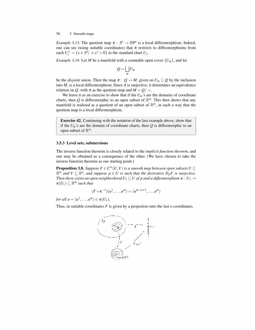
Proposition 3.8. Suppose F 2C•(U,V ) is a smooth map between open subsets U ✓Rm and V ✓ Rn, and suppose p 2 U is such that the derivative DpF is surjective.Then there exists an open neighborhood U1 ✓U of p and a diffeomorphism k : U1 !k(U1)✓ Rm such that

(F �k�1)(u1, . . . ,um) = (um�n+1, . . . ,um)

for all u = (u1, . . . ,um) 2 k(U1).

Thus, in suitable coordinates F is given by a projection onto the last n coordinates.

3.5 Smooth maps of maximal rank 59

Although it belongs to multivariable calculus, let us recall how to get this result fromthe inverse function theorem.

Proof. The idea is to extend F to a map between open subsets of Rm, and then applythe inverse function theorem.

By assumption, the derivative DpF has rank equal to n. Hence it has n linearlyindependent columns. By re-indexing the coordinates of Rm (this permutation is it-self a change of coordinates) we may assume that these are the last n columns. Thatis, writing

DpF =⇣

C,D⌘

where C is the n ⇥ (m � n)-matrix formed by the first m � n columns and D then⇥ n-matrix formed by the last n columns, the square matrix D is invertible. Writeelements x 2 Rm in the form x = (x0,x00) where x0 are the first m�n coordinates andx00 the last n coordinates. Let

G : U ! Rm, x = (x0,x00) 7! (x0,F(x)).

Then the derivative DpG has block form

DpG =

✓Im�n 0

C D

◆,

(where Im�n is the square (m � n)⇥ (m � n) matrix), and is therefore invertible.Hence, by the inverse function theorem there exists a smaller open neighborhoodU1 of p such that G restricts to a diffeomorphism k : U1 ! k(U1)✓ Rm. We have,

G�k�1(u0,u00) = (u0,u00)

for all (u0,u00)2 k(U1). Since F is just G followed by projection to the x00 component,we conclude

F �k�1(u0,u00) = u00.

ut

Again, this result has a version for manifolds:

Theorem 3.3. Let F 2C•(M,N) be a smooth map between manifolds of dimensionsm � n, and suppose p 2 M is such that rankp(F) = n. Then there exist coordinatecharts (U,j) around p and (V,y) around F(p), with F(U)✓V , such that

(y �F �j�1)(u0,u00) = u00

for all u = (u0,u00) 2 j(U). In particular, for all q 2V the intersection

F�1(q)\U

is a submanifold of dimension m�n.

60 3 Smooth maps

Proof. Start with coordinate charts (U,j) around p and (V,y) around F(p) suchthat F(U)✓V . Apply Proposition 3.8 to the map eF = y �F �j�1 : j(U)! y(V ),to define a smaller neighborhood j(U1)✓ j(U) and change of coordinates k so thateF � k�1(u0,u00) = u00. After renaming (U1,k �j|U1) as (U,j) we have the desiredcharts for F . The last part of the theorem follows since (U,j) becomes a submanifoldchart for F�1(q)\U (after shifting j by y(q) 2 Rn). ut

Definition 3.7. Let F 2 C•(M,N). A point q 2 N is called a regular value of F 2C•(M,N) if for all x 2 F�1(q), one has rankx(F) = dimN. It is called a criticalvalue (sometimes also singular value) if it is not a regular value.

Note that regular values are only possible if dimN dimM. Note also that all pointsof N that are not in the image of the map F are considered regular values. We mayrestate Theorem 3.3 as follows:

Theorem 3.4 (Regular Value Theorem). For any regular value q 2 N of a smoothmap F 2C•(M,N), the level set S = F�1(q) is a submanifold of dimension

dimS = dimM�dimN.

Example 3.15. The n-sphere Sn may be defined as the level set F�1(1) of the functionF 2C•(Rn+1,R) given by

F(x0, . . . ,xn) = (x0)2 + · · ·+(xn)2.

The derivative of F is the 1⇥(n+1)-matrix of partial derivatives, that is, the gradient—F :

DpF = (2x0, . . . ,2xn).

For x 6= 0 this has maximal rank. Note that any nonzero real number q is a regularvalue since 0 62 F�1(q). Hence all the level sets F�1(q) for q 6= 0 are submanifolds.

Exercise 43. Let 0 < r < R. Show that

F(x,y,z) = (p

x2 + y2 �R)2 + z2

has r2 as a regular value. (The corresponding level set the 2-torus.)

Example 3.16. The orthogonal group O(n) is the group of matrices A 2 MatR(n)satisfying A> = A�1. We claim that O(n) is a submanifold of MatR(n). To see this,consider the map

F : MatR(n)! SymR(n), A 7! A>A,

where SymR(n) ✓ MatR(n) denotes the subspace of symmetric matrices. We wantto show that the identity matrix I is a regular value of F . We compute the differentialDAF : MatR(n)! SymR(n) using the definition‡

‡ Note that it would have been confusing to work with the description of DAF as a matrix ofpartial derivatives.

3.5 Smooth maps of maximal rank 61

(DAF)(X) =ddt

���t=0

F(A+ tX)

=ddt

���t=0

((A>+ tX>)(A+ tX))

= A>X +X>A.

To see that this is surjective, for A 2 F�1(I), we need to show that for any Y 2SymR(n) there exists a solution of

A>X +X>A = Y.

Using A>A = F(A) = I we see that X = 12 AY is a solution. We conclude that I is a

regular value, and hence that O(n) = F�1(I) is a submanifold. Its dimension is

dimO(n) = dimMatR(n)�dimSymR(n) = n2 � 12

n(n+1) =12

n(n�1).

Note that it was important here to regard F as a map to SymR(n); for F viewed as amap to MatR(n) the identity would not be a regular value.

Exercise 44. In using the regular value theorem we have implicitly assumedthat SymR(n) is a manifold. Prove that this is indeed the case.

Definition 3.8. A smooth map F 2 C•(M,N) is a submersion if rankp(F) = dimNfor all p 2 M.

Thus, for a submersion all level sets F�1(q) are submanifolds.

Example 3.17. Local diffeomorphisms are submersions; here the level sets F�1(q)are discrete points, i.e. 0-dimensional manifolds.

Example 3.18. Recall that CPn can be regarded as a quotient of S2n+1. Using charts,one can check that the quotient map p : S2n+1 ! CPn is a submersion. Hence itsfibers p�1(q) are 1-dimensional submanifolds. Indeed, as discussed before thesefibers are circles. As a special case, the Hopf fibration S3 ! S2 is a submersion.

Remark 3.6. (For those who are familiar with quaternions.) Let H = C2 = R4 bethe quaternion numbers. The unit quaternions are a 3-sphere S3. Generalizing thedefinition of RPn and CPn, there are also quaternion projective spaces, HPn. Theseare quotients of the unit sphere inside Hn+1, hence one obtains submersions

S4n+3 !HPn;

the fibers of this submersion are diffeomorphic to S3. For n = 1, one can show thatHP1 = S4, hence one obtains a submersion

p : S7 ! S4

with fibers diffeomorphic to S3.

62 3 Smooth maps

3.5.4 Example: The Steiner surface

In this section, we will give more lengthy examples, investigating the smoothness oflevel sets.

Example 3.19 (Steiner’s surface). Let S ✓ R3 be the solution set of

y2z2 + x2z2 + x2y2 = xyz.

in R3. Is this a smooth surface in R3? (We use surface as another term for 2-dimensional manifold; by a surface in M we mean a 2-dimensional submanifold.)Actually, we can easily see that it’s not. If we take one of x,y,z equal to 0, then theequation holds if and only if one of the other two coordinates is 0. Hence, the inter-section of S with the set where xyz = 0 (the union of the coordinate hyperplanes) isthe union of the three coordinate axes.

Hence, let us rephrase the question: Letting U ✓R3 be the subset where xyz 6= 0,is S\U is surface? To investigate the problem, consider the function

f (x,y,z) = y2z2 + x2z2 + x2y2 � xyz.

The differential (which in this case is the same as the gradient) is the 1⇥3-matrix

D(x,y,z) f =�

2x(y2 + z2)� yz 2y(z2 + x2)� zx 2z(x2 + y2)� xy�

This vanishes if and only if all three entries are zero. Vanishing of the first entrygives, after dividing by 2xy2z2, the condition

1z2 +

1y2 =

12xyz

;

we get similar conditions after cyclic permutation of x,y,z. Thus we have

1z2 +

1y2 =

1x2 +

1z2 =

1y2 +

1x2 =

12xyz

,

with a unique solution x = y = z = 14 . Thus, D(x,y,z) f has maximal rank (i.e., it is

nonzero) except at this point. But this point doesn’t lie on S. We conclude that S\Uis a submanifold. How does it look like? It turns out that there is a nice answer. First,let’s divide the equation for S\U by xyz. The equation takes on the form

xyz(1x2 +

1y2 +

1z2 ) = 1. (3.11)

The solution set of (??) is cantoned in the set of all (x,y,z) such that xyz > 0. On thissubset, we introduce new variables

a =

pxyzx

, b =

pxyzy

, g =

pxyzz

;

3.5 Smooth maps of maximal rank 63

the old variables x,y,z are recovered as

x = bg, y = ag, z = ab .

In terms of a,b ,g , Equation (3.11) becomes the equation a2+b 2+g2 = 1. Actually,it is even better to consider the corresponding points

(a : b : g) = (1x

:1y

:1z) 2 RP2,

because we could take either square root of xyz (changing the sign of all a,b ,gdoesn’t affect x,y,z). We conclude that the map U ! RP2, (x,y,z) 7! ( 1

x : 1y : 1

z )restricts to a diffeomorphism from S\U onto

RP2\{(a : b : g)| abg = 0}.

The image of the map

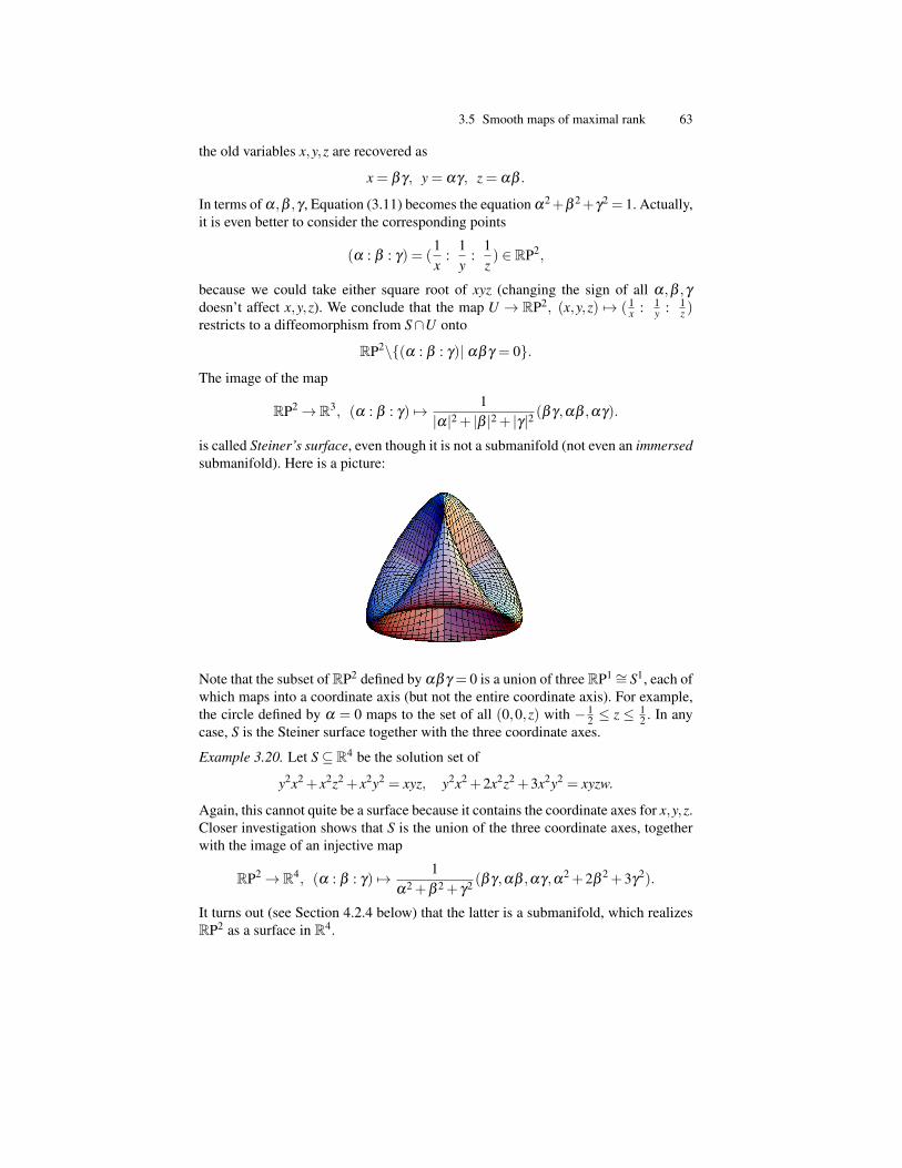
RP2 ! R3, (a : b : g) 7! 1|a|2 + |b |2 + |g|2 (bg,ab ,ag).

is called Steiner’s surface, even though it is not a submanifold (not even an immersedsubmanifold). Here is a picture:

Note that the subset of RP2 defined by abg = 0 is a union of three RP1 ⇠= S1, each ofwhich maps into a coordinate axis (but not the entire coordinate axis). For example,the circle defined by a = 0 maps to the set of all (0,0,z) with � 1

2 z 12 . In any

case, S is the Steiner surface together with the three coordinate axes.

Example 3.20. Let S ✓ R4 be the solution set of

y2x2 + x2z2 + x2y2 = xyz, y2x2 +2x2z2 +3x2y2 = xyzw.

Again, this cannot quite be a surface because it contains the coordinate axes for x,y,z.Closer investigation shows that S is the union of the three coordinate axes, togetherwith the image of an injective map

RP2 ! R4, (a : b : g) 7! 1a2 +b 2 + g2 (bg,ab ,ag,a2 +2b 2 +3g2).

It turns out (see Section 4.2.4 below) that the latter is a submanifold, which realizesRP2 as a surface in R4.

64 3 Smooth maps

3.5.5 Immersions

We next consider maps F : M ! N of maximal rank between manifolds of dimen-sions m n. Once again, such a map can be put into a ‘normal form’: By choosingsuitable coordinates it becomes linear.

Proposition 3.9. Suppose F 2C•(U,V ) is a smooth map between open subsets U ✓Rm and V ✓Rn, and suppose p 2U is such that the derivative DpF is injective. Thenthere exist smaller neighborhoods U1 ✓U of p and V1 ✓V of F(p), with F(U1)✓V1,and a diffeomorphism c : V1 ! c(V1), such that

(c �F)(u) = (u,0) 2 Rm ⇥Rn�m

Proof. Since DpF is injective, it has m linearly independent rows. By re-indexing therows (which amounts to a change of coordinates on V ), we may assume that theseare the first m rows.

That is, writing

DpF =

✓AC

◆

where A is the m⇥m-matrix formed by the first m rows and C is the (n�m)⇥m-matrix formed by the last n�m rows, the square matrix A is invertible. Consider themap

H : U ⇥Rn�m ! Rn, (x,y) 7! F(x)+(0,y)

ThenD(p,0)H =

✓A 0C In�m

◆

is invertible. Hence, by the inverse function theorem for Rn, H is a diffeomorphismfrom some neighborhood of (p,0) in U ⇥Rn�m onto some neighborhood V1 ofH(p,0) = F(p), which we may take to be contained in V . Let

3.5 Smooth maps of maximal rank 65

c : V1 ! c(V1)✓U ⇥Rn�m

be the inverse; thus(c �H)(x,y) = (x,y)

for all (x,y) 2 c(V1). Replace U with the smaller open neighborhood

U1 = F�1(V1)\U

of p. Then F(U1)✓V1, and

(c �F)(u) = (c �H)(u,0) = (u,0)

for all u 2U1. ut

The manifolds version reads as follows:

Theorem 3.5. Let F 2C•(M,N) be a smooth map between manifolds of dimensionsm n, and p 2 M a point with rankp(F) = m. Then there are coordinate charts(U,j) around p and (V,y) around F(p) such that F(U)✓V and

(y �F �j�1)(u) = (u,0).

In particular, F(U)✓ N is a submanifold of dimension m.

Proof. Once again, this is proved by introducing charts around p, F(p) to reduce toa map between open subsets of Rm, Rn, and then use the multivariable version of theresult to obtain a change of coordinates, putting the map into normal form. ut

Definition 3.9. A smooth map F : M ! N is an immersion if rankp(F) = dimM forall p 2 M.

Example 3.21. Let J ✓ R be an open interval. A smooth map g : J ! M is alsocalled a smooth curve. We see that the image of g is an immersed submanifold,provided that rankp(g) = 1 for all p 2 M. In local coordinates (U,j), this means thatddt (j � g)(t) 6= 0 for all t with g(t) 2U . For example, the curve g(t) = (t2, t3) fails tohave this property at t = 0.

Example 3.22 (Figure eight). The map

g : R! R2, t 7!�

sin(t),sin(2t)�

is an immersion; the image is a figure eight.

66 3 Smooth maps

(Indeed, for all t 2 R we have Dtg ⌘ g(t) 6= 0.)

Example 3.23 (Immersion of the Klein bottle). The Klein bottle admits a ‘figureeight’ immersion into R3, obtained by taking the figure eight in the x � z-plane,moving in the x-direction by R > 1, and then rotating about the z-axis while at thesame time rotating the figure eight, so that after a full turn j 7! j + 2p the figureeight has performed a half turn.

We can regard this procedure as a composition of the following maps:

F1 : (t,j) 7! (sin(t),sin(2t),j) = (u,v,j),

F2 : (u,v,j) 7!⇣

ucos(j2)+ vsin(

j2), vcos(

j2)�usin(

j2),j

⌘= (a,b,j)

F3 :�a,b,j) 7! ((a+R)cosj, (a+R)sinj, b

�= (x,y,z).

Here F1 is the figure eight in the u� v-plane (with j just a bystander). F2 rotatesthe u� v-plane as it moves in the direction of j , by an angle of j/2; thus j = 2pcorresponds to a half-turn. The map F3 takes this family of rotating u,v-planes, andwraps it around the circle in the x� y-plane of radius R, with j now playing the roleof the angular coordinate.

The resulting map F = F3 �F2 �F1 : R2 ! R3 is given by F(t,j) = (x,y,z),where with

x =⇣

R+ cos(j2)sin(t)+ sin(

j2)sin(2t)

⌘cosj,

y =⇣

R+ cos(j2)sin(t)+ sin(

j2)sin(2t)

⌘sinj,

z = cos(j2)sin(2t)� sin(

j2)sin(t)

is an immersion. To verify that this is an immersion, it would be cumbersome towork out the Jacobian matrix directly. It is much easier to use that F is obtained asa composition F = F3 �F2 �F1 of the three maps considered above, where F1 is animmersion, F2 is a diffeomorphism, and F3 is a local diffeomorphism from the opensubset where |a|< R onto its image.

Since the right hand side of the equation for F does not change under the trans-formations

3.5 Smooth maps of maximal rank 67

(t,j) 7! (t +2p,j), (t,j) 7! (�t,j +2p),

this descends to an immersion of the Klein bottle. It is straightforward to checkthat this immersion of the Klein bottle is injective, except over the ‘central circle’corresponding to t = 0, where it is 2-to-1.

Note that under the above construction, any point of the figure eight creates acircle after two‘full turns’, j 7! j +4p . The complement of the circle generated bythe point t = p/2 consists of two subsets of the Klein bottle, generated by the partsof the figure eight defined by �p/2 < t < p/2, and by p/2 < t < 3p/2. Each ofthese is a ‘curled-up’ immersion of an open Mobius strip. (Remember, it is possibleto remove a circle from the Klein bottle to create two Mobius strips!) The point t = 0also creates a circle; its complement is the subset of the Klein bottle generated by0 < t < 2p . (Remember, it is possible to remove a circle from a Klein bottle to createone Mobius strip.) We can also remove one copy of the figure eight itself; then the‘rotation’ no longer matters and the complement is an open cylinder. (Remember, itis possible to remove a circle from a Klein bottle to create a cylinder.)

Example 3.24. Let M be a manifold, and S ✓ M a k-dimensional submanifold. Thenthe inclusion map i : S ! M, x 7! x is an immersion. Indeed, if (V,y) is a subman-ifold chart for S, with p 2U =V \S, j = y|V\S then

(y �F �j�1)(u) = (u,0),

which shows thatrankp(F) = rankj(p)(y �F �j�1) = k.

By an embedding, we will mean an immersion given as the inclusion map for asubmanifold. Not every injective immersion is an embedding; the following picturegives a counter-example:

In practice, showing that an injective smooth map is an immersion tends to be easierthan proving that its image is a submanifold. Fortunately, for compact manifolds wehave the following fact:

Theorem 3.6. If M is a compact manifold, then every injective immersion F : M !Nis an embedding as a submanifold S = F(M).

Proof. Let p 2 M be given. By Theorem 3.5, we can find charts (U,j) around pand (V,y) around F(p), with F(U) ✓ V , such that eF = y �F �j�1 is in normalform: i.e., eF(u) = (u,0). We would like to take (V,y) as a submanifold chart forS = F(M), but this may not work yet since F(M)\V = S\V may be strictly larger

68 3 Smooth maps

than F(U)\V . Note however that A := M\U is compact, hence its image F(A) iscompact, and therefore closed (here we are using that N is Haudorff). Since F isinjective, we have that p 62 F(A). Replace V with the smaller open neighborhoodV1 =V\(V \F(A)). Then (V1,y|V1) is the desired submanifold chart.

Remark 3.7. Some authors refer to injective immersions i : S!M as ‘submanifolds’(thus, a submanifold is taken to be a map rather than a subset). To clarify, ‘our’ sub-manifolds are sometimes called ‘embedded submanifolds’ or ‘regular submanifolds’.

Example 3.25. Let A,B,C be distinct real numbers. We will leave it as a homeworkproblem to verify that the map

F : RP2 ! R4, (a : b : g) 7! (bg,ag,ab , Aa2 +Bb 2 +Cg2),

where we use representatives (a,b ,g) such that a2 + b 2 + g2 = 1, is an injectiveimmersion. Hence, by Theorem 3.6, it is an embedding of RP2 as a submanifold ofR4.

To summarize the outcome from the last few sections: If F 2C•(M,N) has max-imal rank near p 2 M, then one can always choose local coordinates around p andaround F(p) such that the coordinate expression of F becomes a linear map of maxi-mal rank. (This simple statement contains the inverse and implicit function theoremsfrom multivariable calculus are special cases.)

Remark 3.8. This generalizes further to maps of constant rank. In fact, if rankp(F)is independent of p on some open subset U , then for all p 2 U one can choosecoordinates in which F becomes linear.