3344 IEEE TRANSACTIONS ON IMAGE PROCESSING, VOL. 26, NO. …decsai.ugr.es/vip/files/journals/07875464.pdf · 3344 IEEE TRANSACTIONS ON IMAGE PROCESSING, VOL. 26, NO. 7, JULY 2017

3344 IEEE TRANSACTIONS ON IMAGE PROCESSING, VOL. 26, NO. 7, JULY 2017

Bayesian K-SVD Using Fast Variational InferenceJuan G. Serra, Matteo Testa, Rafael Molina, and Aggelos K. Katsaggelos, Fellow, IEEE

Abstract— Recent work in signal processing in general andimage processing in particular deals with sparse representa-tion related problems. Two such problems are of paramountimportance: an overriding need for designing a well-suitedovercomplete dictionary containing a redundant set of atoms—i.e., basis signals—and how to find a sparse representation ofa given signal with respect to the chosen dictionary. Dictio-nary learning techniques, among which we find the popularK-singular value decomposition algorithm, tackle these problemsby adapting a dictionary to a set of training data. A commondrawback of such techniques is the need for parameter-tuning.In order to overcome this limitation, we propose a fully-automated Bayesian method that considers the uncertainty ofthe estimates and produces a sparse representation of the datawithout prior information on the number of non-zeros in eachrepresentation vector. We follow a Bayesian approach that usesa three-tiered hierarchical prior to enforce sparsity on therepresentations and develop an efficient variational inferenceframework that reduces computational complexity. Furthermore,we describe a greedy approach that speeds up the whole process.Finally, we present experimental results that show superiorperformance on two different applications with real images:denoising and inpainting.

Index Terms— Bayesian modeling, sparse representation,k-svd, variational inference, dictionary learning, denoising,inpainting.

I. INTRODUCTION

S IGNAL representation has drawn a lot of attention inthe last decades. Be it a 1D signal, an image or a

video, such representations should capture the most significantcharacteristics of the signal. These depend heavily on theapplication but seem to find a common goal in simplicitynonetheless.

Representing a signal requires the selection of a dictionary,i.e., a set of “atoms” or vectors in the signal space, a linear

Manuscript received December 14, 2015; revised August 14, 2016and November 21, 2016; accepted February 22, 2017. Date of publicationMarch 10, 2017; date of current version May 16, 2017. This work wassupported by the Spanish Ministry of Economy and Competitiveness underProject TIN2013-43880-R and Project DPI2016-77869-C2-2-R, in part bythe Department of Energy under Grant DE-NA0002520, and in part bythe European Research Council under the European Communitys SeventhFramework Programme (FP7/2007-2013) under Grant 279848. The associateeditor coordinating the review of this manuscript and approving it forpublication was Prof. Ling Shao. (Juan G. Serra and Matteo Testa contributedequally to this work.)

J. G. Serra and R. Molina are with the Deptartmento de Ciencias de laComputación e I. A., University of Granada, 18071 Granada, Spain (e-mail:[email protected]; [email protected]).

M. Testa is with the Department of Electronics and Telecommunications,Politecnico di Torino, 10129 Turin, Italy (e-mail: [email protected]).

A. K. Katsaggelos is with the Department of Electrical Engineeringand Computer Science, Northwestern University, Evanston, IL 60208 USA(e-mail: [email protected]).

Color versions of one or more of the figures in this paper are availableonline at http://ieeexplore.ieee.org.

Digital Object Identifier 10.1109/TIP.2017.2681436

combination of which represents the given signal (alternativerepresentations based on the use of manifolds [1], [2] arealso relevant but will not be discussed here). The obvious andsimplest choice of a dictionary is a basis, the smallest possibledictionary with the capability of representing the whole signalspace. Simple as they are, the scarce expressiveness of suchdictionaries led to the ongoing development of overcompletedictionaries [3].

The transition to overcomplete dictionaries was gradual.Analytical complete dictionaries were introduced first, whichmade use of different transforms such as DCT, Wavelet orGabor. The limitations of such transforms were soon broughtto light. Indeed, the work in [4] pointed out the deficienciesof the popular orthogonal wavelet transforms, namely itssensitivity to translation, dilation and rotation, resulting inthe development of the Steerable Wavelet Transform. Earlyapproaches towards overcomplete dictionaries tried to preservethe favorable orthogonality properties of bases but soon provedto be insufficient.

Parallel work suggested the use of collections of data tobetter describe signals, rather than the use of mathematicalartificial functions. The works in [5] and [6] were veryinfluential towards the recent advances in dictionary learningand sparse signal representation.

Let us now introduce the dictionary learning problem in amore formal way: we aim to find a sparse representation ofeach signal in a database of Q natural signals to R

P con-catenated column-wise into a matrix as Y = [

y1, · · · , yQ] ∈

RP×Q . We do this by finding a set of K atoms in the signals’

ambient space, concatenated into a dictionary matrix D =[d1, · · · , dK ] ∈ R

P×K . This dictionary, and the correspondingassignment matrix X = [x1, · · · , xQ ] ∈ R

K×Q for the signals,are recovered by solving an optimization problem where weseek the best reconstruction of our signals given a budget Tfor the number of non-zero entries allowed in each column ofX. Formally this problem takes the form

minD,X

‖Y − DX‖2F

s.t. ‖xq‖0 ≤ T, q = 1, . . . , Q, (1)

where ‖ · ‖0 denotes the �0-(pseudo)norm, which counts thenon-zero entries in a vector, and ‖ · ‖F denotes the Frobeniusnorm.

Since the objective function ‖Y − DX‖2F is not convex in

X and D jointly, but biconvex, that is, convex in X and Dindividually, this problem can be addressed by alternatingminimization over each variable separately. However, theexact minimization over X is well known to be NP-hard.Therefore greedy methods, among which the popular K-SVD

1057-7149 © 2017 IEEE. Personal use is permitted, but republication/redistribution requires IEEE permission.See http://www.ieee.org/publications_standards/publications/rights/index.html for more information.

SERRA et al.: BAYESIAN K-SVD USING FAST VARIATIONAL INFERENCE 3345

algorithm [7], are used to approximate the true solution.Alternatively, the sparsity constraint can be relaxed, resultingin the following problem

minD,X

‖Y − DX‖2F

s.t. ‖xq‖1 ≤ T, q = 1, . . . , Q, (2)

where ‖ · ‖1 denotes the vector �1-norm. A wide array oftechniques from convex optimization can be applied to solvethis problem (e.g., [7]–[10]).

The dictionary learning problem (in both forms of (1)and (2)) has been widely applied in image processingand machine learning. Applications include image denois-ing and deblurring [11], [12], image super-resolution [13],image restoration [14], face recognition [15], and classifica-tion [16] among many others. Focusing on this latter category,Vu et al. [17] propose to perform histopathological imageclassification through the use of class-specific dictionaries.In more detail, a class-specific dictionary should be able tocorrectly sparsify a signal belonging to the related class byemploying just few atoms in the representation, but it shouldrepresent poorly a signal belonging to a different class. Thus,the classification is performed by analyzing the usage of atomsin the different dictionaries.

Back to the general dictionary learning problem, an alter-native approach to the problem it is studied in the workof Skretting and Engan [18], referred to as the RecursiveLeast Squares Dictionary Learning Algorithm (RLS-DLA),according to which a continuous update of the dictionary isperformed after each training vector is processed. Thereinlies the main difference between RLS-DLA and other pre-vious approaches such as its precedent ILS-DLA [19] orK-SVD [7]. However, its convergence has not been estab-lished. Liu et al. [20] propose a different method for theestimation of D and X using a two-level Bregman-based tech-nique for MRI reconstruction. Its inner loop updates the sparsecoefficients following an iterative shrinkage/thresholding algo-rithm, whereas the outer loop basically updates the atoms ofthe dictionary, which consists of a refinement of the previ-ous one, involving just a matrix multiplication. A follow-uppublication by Liu et al. [21], further validates their previouslypresented method applying sparse representations to the imagedeconvolution problem.

For what concerns deterministic techniques for dictionarylearning, another popular approach is the analysis approach.In contrast to the standard synthesis method in which theemphasis is placed on the signal decomposition by means oflinear combinations of few atoms of a given dictionary, inthe analysis counterpart the dictionary represents an operatorwhich, multiplied by the signals, results in a sparse outcome.Examples of works following this approach include [22]and [23].

Along with deterministic methods to solve the dictionarylearning problem, probabilistic approaches have also beenproposed. In their seminal works, Olshausen and Field [6] andLewicki and Sejnowski [24] introduced a generative modelfor the data which allowed them to develop a MaximumLikelihood (ML) estimator for both the sparse coding and

the dictionary. According to this model, when the prior onthe sparse signal is a heavily peaked Laplacian distributionaround zero and the residual is approximated by a zero-mean Gaussian distribution, the dictionary learning problemreduces to the one in (2). Following this work, other authorsproposed modifications to either the sparse approximationstep, the dictionary update, or both. In [25], using the samegenerative model introduced in [6], Ramirez et al. proposedthe use of Orthogonal Matching Pursuit (OMP) to solve thesparse coding problem and a closed form solution for thedictionary update equation. Later papers focused on the useof a Maximum a Posteriori (MAP) approach instead, whichallows to impose constraints on the dictionary as well. Forinstance, in the work of Kreutz-Delgado et al. [26] a unit-norm Frobenius prior is placed on the dictionary. However,due to the intractability of such a prior, they propose to usean approximate solution and the FOCUSS [27] algorithm inorder to obtain the sparse solution. Other choices of priorsinvolve smoother (less sparse) priors based on the Kullback-Leibler divergence for the �1 regularization as in [28]. Theadvantage of this latter approach lies in the increased stabilityof the sparse solution and the efficient convex inference.

All of the aforementioned techniques use ML or MAPestimators to solve the dictionary learning problem. However,the main drawback of such approaches is that they do nottake into account the uncertainty of the estimated sparserepresentation coefficients, which, as we will later examine,leads to reduced algorithmic performance. Moreover, since thevariance of the noise is not explicitly taken into account inthe model, these algorithms have to rely on other techniquesfor noise estimation. The importance of a good estimate ofthe noise variance is discussed in [9] where the authors showthat when using K-SVD for image denosing [11], the resultingPSNR is highly affected by the precision of the noise varianceestimate.

To overcome these problems a few techniques have beendeveloped. These include the incorporation of the noise vari-ance/covariance information in the model as a parameter thatcan be estimated and taking into account the uncertainty ofthe estimates. Girolami [29] propose an Expectation Maxi-mization (EM) algorithm in which the posterior of the sparsesignal is estimated along with the dictionary. In more detail,each column of X is modeled using a Laplacian prior which,however, leads to an intractable posterior distribution, forwhich the authors propose to use a variational approximationof the prior which tranforms the posterior of the sparse signalinto a Gaussian form. Finally, an EM algorithm is developedin order to estimate the parameters of the model. However,with this approach, the authors do not place a prior on theentries of the dictionary.

Zhou et al., [9] and [30], utilize a Beta-Bernoulli prior forthe selection of the active-set, employing the Beta ProcessFactor Analysis (BPFA) modeling introduced in [31]. Theactive-set is the smallest possible set of atoms in the dictionarywhich is capable of efficiently explaining the underlyingsignal structure. Similarly to [32], the model can also beused to estimate the size of the dictionary. In addition, theauthors introduced a Dirichlet patch clustering in order to


group the data which have the same probability of beingrepresented using a fixed set of atoms. Samples from the fullposterior distribution are obtained through Gibbs sampling.BPFA modeling is also used in [33]. In this work, the prob-lem of MRI image reconstruction from Compressed Sensingmeasurements is tackled with the introduction of a TotalVariation (TV) penalty term in the functional, which is thensolved through the use of the Alternating Direction Methodof Multipliers (ADMM). The BPFA modeling falls into thecategory of the so-called Spike and Slab (SnS) prior models.The main idea of this technique is to introduce a binaryvector for the selection of the variables to be included inthe model as in [34], where authors use this prior on thelinear regression coefficients. This modeling is particularlyuseful when the number of observations is smaller than thenumber of possible predictors. The presence of the Diracdelta function in the model makes inference a difficult task.Authors have addressed this issue in several manners. Bayesianvariational inference is used on SnS based models in [35],where a reparametrization of the SnS prior is proposed.The novelty of the work lies in a new factorization thanksto which each factor is a mixture of two Gaussians. Theauthors also show the effectiveness of such approach withrespect to standard factorization as in [36], where the posteriorapproximation of the factors is a mixture of components witha single (unimodal) Gaussian distribution, which leads to aless accurate representation of the data. Based on this model,and motivated by the fact that posterior independence results inorthogonality of inferred atoms, [37] introduces an ExpectationMaximization approach which does not assume independenceamong the dictionary elements. To efficiently deal with largedatasets, the model in [30] was adapted to process randomlypartitioned data in [38]. In more detail, the parameters ofthe model are inferred locally for each set of partitioneddata and then aggregated using a weighted average to updatethe global parameters of the model resulting in an increasedrobustness to local minima and reduced memory requirements.Andersen et al. [39] propose a novel structured SnS priorwhich allows to incorporate prior knowledge on the sup-port of the coefficient vectors via a Gaussian Process (GP)over the SnS probabilities; a later extension of theirwork, [40], covers the inference of the GP parameters. TheGP models the sparsity patterns and considers correlationsbetween the SnS probabilities of different coefficient vectors.Mousavi et al. [41] use a variant of SnS that replaces the Diracdelta function by an indicator function, based on the MAPestimation technique proposed in [42]. It allows to infer theoptimal sparse coefficients by solving an optimization problemwithout relaxation. Finally, the work by Y. Zhang et al. [43]also utilizes the Bernoulli prior on the binary activationsbut imposes a multiplicative Gaussian process on the 2Dcoordinates of the image patches which enforces similarity onthe support of neighboring patches. Furthermore, uncorrelationamong dictionary atoms is favored by the use of a SigmoidBelief Network.

Note that using variational inference on SnS priors, see forinstance, [30] and [35], may not lead to an exact sparse solu-tion since computing the expectation over a binary distribution

will not necessarily produce a binary {0, 1} value. However,this can be easily solved by using the thresholding approachin [38]. The method we propose in this work also leads toexact sparse solutions since it allows atoms to be added orremoved completely from the model.

Additionally, we can find Dictionary Learning and SparseCoding approximations which seek overall acceleration of theprocess. The works Gregor and LeCun et al. use a multi-layer feed forward network [44] or a binary tree [45] whichmake the algorithms suitable for real-time visual applications,such as object recognition. Along with these approximationtechniques, [46] presents three different Dictionary Learningalgorithms which also focus on computational efficiency. Theauthors propose partial updating of the atoms to accelerateconvergence, a one-stage procedure in which each atom isupdated along with its corresponding row in the coefficientmatrix, letting the non-zero entries change, contrary to K-SVD,and lastly they incorporate the FISTA [47] sparse coding stageto the latter for faster performance.

Works which analyze the theoretical limits of the dictio-nary learning approach can also be found in the literature.In particular, Gribonval et al. [48] analyze the local minima ofthe non-convex functional in the dictionary learning problem.The results they obtain show that with high probability thesparse coding admits a local minimum around the dictionarywhich generated the signals. Additionally, C. Bao et al. [49]present a multi-block alternating proximal method with provenglobal convergence which is faster than K-SVD with similarperformance.

In this work we propose a novel Bayesian algorithm forsolving the �1 dictionary learning problems. Our approachaims at estimating the whole posterior distribution of X(thus taking into account the uncertainty of the estimatedcoefficients) but with an automatic technique for the estima-tion of the parameters which originate with the introducedmodels. The proposed approach is applied to image denoisingand inpainting in order to test its performance in differentapplications of interest in image processing.

The paper is organized as follows. In Section II we brieflydescribe the K-SVD algorithm. Section III presents a hierar-chical Bayesian model based on the use of the Laplace prior,and in Section IV we provide the details of the inferenceprocedure to estimate the unknowns. Based on the infer-ence procedure in Section IV, we develop a computation-ally efficient implementation based on Empirical Bayes inSection V-A. Numerical examples demonstrating the effec-tiveness of the proposed algorithm are given in Section VI,where we compare the results with state-of-the-art alternatives.Finally, we draw concluding remarks in Section VII.

Notation: Unless otherwise noted, throughout this paper,we use boldface upper-case and lower-case letters to denotematrices and vectors, respectively. For a matrix X, its i thcolumn and j th row are denoted by xi and x j , respectively.The (i, j)-th entry of a matrix X is denoted by either xi j orX(i, j), whichever makes the notation clearer. Given a vectorx, diag(x) represents the square matrix with the entries of x onits diagonal, while given a square matrix X, diag(X) extractsits diagonal into a vector. Given a square matrix X, Tr(X) and


|X| denote the trace and determinant operators, respectively.The M × 1 all-zero vector is denoted by 0M , and finally, theM × M identity matrix is denoted by IM .

II. THE K-SVD ALGORITHM

Among the most popular algorithms for dictionary learning,K-SVD [7] is a greedy approach that approximately solvesthe standard �0 problem in (1). In K-SVD the optimization isperformed coordinate-wise alternating between X and D.

At each iteration of the K-SVD algorithm, given the currentstate update of the dictionary, the Orthogonal Matching Pursuit(OMP) algorithm [50] is first applied to determine the supportof X, i.e., the locations of the non-zeros in X, while the valuesat these non-zero locations obtained from OMP are discarded.Notice that this requires manually fixing the number of non-zero components in each column of X.

After OMP, D and the non-zeros of X are updated. The termDX can be decomposed as

DX =K∑

k=1

dkxk . (3)

This decomposition forms the basis of a cyclic update proce-dure, where each pair of {(dk, xk)}K

k=1 is updated individuallywhile all other pairs are held constant at their most recentvalues. Specifically, for the j th pair, the objective function in(1) can be expressed as the sum of a residual and a rank-onematrix, i.e.,

mind j ,x j

‖Y − DX‖2F = min

d j ,x j‖R j − d j x j‖2

F, (4)

where the residual term

R j = Y −∑

i �= j

di xi (5)

does not depend on (d j , x j ). Because d j x j has at mostrank one, the minimization in (4) is precisely a low-rankapproximation problem, which can be solved via the SingularValue Decomposition (SVD) [51].

Before computing the SVD of R j , we note that the supportof X has already been determined using OMP. Resetting x j viathe SVD of R j would destroy its sparse structure. To resolvethis issue, instead of considering R j , we consider R j , whichis formed by retaining the columns of R j that correspond tothe non-zero entries in x j . As we will see later, this restrictedprocessing has a clear justification in the Bayesian context.Concretely, we have

d j x j = σ1u1v1, (6)

where σ1 is the largest singular value of R j , u1 and v1 are itscorresponding left and right singular vectors, and x j denotesthe row vector x j after imposing the known sparsity support.After this step, the values at the non-zero locations of x j are setequal to x j . Notice that this restricted non-zero update does nothave a mathematical justification and will reduce the qualityof the SVD fitting. A justified way to alternate between atomand representation updates will be proposed in the comingsections.

The advantage of the K-SVD algorithm is its simplicity, asthe update steps are greedy in nature. One major drawback,though, is that the uncertainty of the estimates of D and Xis not taken into account in the estimation procedure. Whilenot taking into account the uncertainty in the atoms of Dmay not be a problem due to the generally large numberof columns in X, each column of X normally has a reducednumber of non-zero components and their inherent uncertaintyshould be accounted for. Furthermore, K-SVD requires toknow the number of non-zero components in each columnof X, information that may not be available or may evenbe column dependent. In this paper we will show how theseproblems can be tackled in a principled manner using Bayesianmodeling and inference.

III. HIERARCHICAL BAYESIAN MODEL

A. Noise Modeling

The use of the sparsity inducing �1 norm in (2) requires anelaborate modeling. Following our previous work in [52], webegin by modeling the observation process by using

p(Y|D, X, β) ∝ βP Q2 exp

{−β

2‖Y − DX‖2

F

}, (7)

where β is the noise precision. We assume that

p(β|aβ, bβ) = �(β|aβ, bβ) ∝ βaβ−1 exp(−bββ), (8)

with aβ > 0 and bβ > 0 being the shape and inverse scaleparameters, respectively.

B. Modeling of D and X

Since we expect the columns of D to be normalized vectors,we utilize the following prior on D

p(D) =K∏

k=1

p(dk) (9)

where

p(dk) ={

const if ‖ dk ‖= 1

0 elsewhere(10)

We now proceed to model the columns of X. Althoughvarious general sparsity promoting priors could be consideredhere, see [53], we will only investigate the use of the Laplaceprior on the components of the columns of X in this paper.The non-conjugacy of the likelihood in (7) and Laplace priordistributions makes the use of this prior for the columns of Xintractable. In our approach we address this issue by applyinginstead a three-tiered hierarchical prior on each column of X,which has the same sparsifying effect as a Laplace prior whilerendering the inference tractable.

For each column xq , q = 1, . . . , Q of X, we utilize

p(xq |γq) =K∏

k=1

N (xkq |0, γkq)

= N (xq |0K ,�q) (11)


where γq is a K × 1 column vector with elements γkq , k =1, · · · , K , and �q = diag(γq ) along with the tiered hyperpriors

p(γq |λq) =K∏

k=1

�(γkq |1, λq/2) (12)

and

p(λq |νq) = �(λq |νq/2, νq/2), (13)

where we assume a flat distribution on νq .With marginalization, this hierarchical model yields a

Laplace distribution of xq conditioned on λq

p(xq |λq

) = λK/2q

2Kexp

{−√λq‖xq‖1

}. (14)

C. Complete System Modeling

Throughout the remainder of this paper we will denote by

� = [γ1, · · · , γQ

], λ = [

λ1, · · · , λQ], ν = [

ν1, · · · , νQ]

(15)

the hyperparameters associated with X.We also denote the entire set of unknowns as

� ={{dk}K

k=1, {xq}Qq=1,�,λ, ν, β

}. (16)

Based on the above presented modeling, the completesystem modeling is therefore given by the joint distribution

p(Y,�) = p(Y|D, X, β)p(β)p(D)p(X|�)p(�|λ)p(λ|ν)p(ν).

(17)

IV. INFERENCE

Our scheme for estimating D and X depends on our abilityto estimate the posterior distribution p (�|Y). We do this usingvariational distribution approximation [54]. Specifically, withMean-Field Factorization, the joint posterior distribution isapproximated as

q (�) = q(β)q (�) q (λ) q(ν)q(X)∏K

k=1 q(dk), (18)

where in our case it is assumed that q (�), q (λ), and q(ν) aredegenerate distributions. We also assume that each q(dk), k =1, . . . , K is a degenerate distribution on a vector with ‖dk ‖2= 1.

For each θi ∈ � where q(θi ) is assumed to be degenerate,we can update its value by calculating

θi = arg maxθi

ln q (θi ) = arg maxθi

〈ln p (Y,�)〉�\θi, (19)

where 〈·〉�\θi denotes the expectation taken with respect to allapproximating factors q(θ j ), j �= i .

For each θi where q(θi ) is assumed to be non-degenerate,we apply calculus of variations and obtain

ln q (θi ) = 〈ln p (Y,�)〉�\θi+ C, (20)

where C denotes a constant independent of the variable ofcurrent interest. For non-degenerate distributions q(θi ), theupdated value θi will denote its mean.

A. Estimation of X, �, λ, and ν

In order to find an approximate posterior distribution of X,we apply (20) and obtain

ln q(X) = 〈ln p(Y|D, X, β) + ln p(X|�)〉�\X + C

=Q∑

q=1

⟨−β

2

∥∥yq − Dxq

∥∥2

2 − 1

2xT

q �−1q xq

⟩

�\xq

+ C

=Q∑

q=1

{

− β

2

∥∥∥yq − Dxq

∥∥∥

2

2− 1

2xT

q �−1q xq

}

+ C.

(21)

It is clear from (21) that the columns of X in the posteriordistribution approximation are independent with

ln q(xq) = − β

2‖yq − Dxq‖2

2 − 1

2xT

q �−1q xq + C. (22)

It is straightforward to see that q(xq) is a Gaussian distrib-ution

q(xq) = N (xq |xq,�xq ) (23)

with covariance matrix and mean vector defined respectivelyas

�xq =(βDTD + �−1

q

)−1(24)

xq = β�xq DTyq . (25)

Next, taking the appropriate expectation and finding asolution to (19) we can calculate the updates for the hyperpa-rameters associated with X

For γq we have the following optimization problem

γq = arg maxγq

〈ln p (Y,�)〉�\γq

= arg maxγq

〈ln p(xq |γq

)p(γq |λq

)〉xq ,λq + C, (26)

where C contains all the terms which do not involve γq . Using(11) and (12), we have

〈ln p (Y,�)〉�\γq = −1

2

K∑

k=1

log γkq − 1

2〈xT

q �−1q xq〉xq

+ K log λq − λq

2

K∑

k=1

γkq + C, (27)

where

〈xTq �−1

q xq〉 = 〈xq 〉T �−1q 〈xq 〉 + tr(�xq �

−1q ). (28)

We now find the optimal γkq by setting the derivative of theprevious expression with respect to γkq equal to zero, whichyields:

γkq = − 1

2λq+

√√√√ 1

4λ2q

+ x2kq + �xq (k, k)

λq. (29)

Following an analogous procedure, we have that

λq = arg maxλq

〈ln p (Y,�)〉�\λq

= arg maxλq

〈ln p(γq |λq

)p(λq |νq

)〉γq ,νq + C. (30)


Again, expanding the previous expression using (12) and (13)we obtain

〈ln p (Y,�)〉�\λq = K log λq − λq

2

K∑

k=1

γkq (31)

+(

νq

2−1

)log λq − νq

2λq +C, (32)

and maximizing, the optimal λq is given by

λq = νq + 2K − 2

νq +K∑

k=1γkq

. (33)

Finally, for νq we have

νq = arg maxνq

〈ln p (Y,�)〉�\νq

= arg maxνq

〈ln p(λq |νq

)p〉λq + C,

which, after using (13), produces

νq

2ln

νq

2− ln

(�(νq

2

))+ νq

2

(ln λq − λq

). (34)

This formula does not allow for an analytical solution, requir-ing numerical optimization to find the optimal νq .

B. Estimation of D

First notice that we assume that the columns of D areindependent of each other in the posterior distribution approx-imation, i.e.,

q(D) =K∏

k=1

q(dk) , (35)

with these distributions degenerate on a point in ‖ dk ‖= 1.Focusing on a single dk and applying (19), we have

dk = arg mindk

⟨‖Y − DX‖2

F

⟩

�\dk

s.t . ‖ dk ‖= 1. (36)

We can write

〈‖Y − DX‖2F〉�\dk = 〈‖Y − DX + D(X − X)‖2

F〉�\dk

= 〈‖Y−DX‖2F〉�\dk +〈‖D(X−X)‖2

F〉�\dk

(37)

where the cross terms are not included since both are identicaland equal to zero. For the first term we have

〈‖Y − DX‖2F〉�\dk = ‖Y −

∑

i �=kdi xi − dk xk‖2

F

= ‖xk‖22dT

k dk − 2bTk dk + C (38)

with

bk = (Y −∑

i �=kdi xi )(xk)T. (39)

Notice that (38) is the only term used in K-SVD to update theatoms of the dictionary.

The uncertainty of the estimate of xq is incorporated in theestimation of dk by the second term on the right hand side of(37) which we now calculate. It can be expressed as

〈‖D(X − X)‖2F〉�\dk

= 〈‖dk(xk − xk)‖2F〉�\dk

+2〈Tr(dk(xk − xk)(∑

i �=k

di (xi − xi ))T)〉�\dk + C. (40)

Now, the first term on the right hand side of (40) can bewritten as

〈‖dk(xk − xk)‖2F〉�\dk = ckdT

k dk, (41)

where

ck = 〈‖xk − xk‖22〉�\dk = 〈

Q∑

q=1

(xkq − xkq )2〉�\dk

=Q∑

q=1

�xq (k, k), (42)

and �xq (k, k) denotes the (k, k)-th element of �xq defined in(24).

Similarly, the second term on the right hand side of (40)can be written as

〈Tr(dk(xk − xk)(∑

i �=k

di (xi − xi ))T)〉�\dk

= 〈(xk − xk)(∑

i �=k

(xi − xi )TdTi )〉�\dk dk

=∑

i �=k

〈(xk − xk)(xi − xi )TdTi 〉�\dk dk = aT

k dk, (43)

where

ak =Q∑

q=1

∑

i �=k

�xq (i, k)di . (44)

Substituting (41) and (43) into (40), we obtain

〈‖D(X − X)‖2F〉�\dk = ckdT

k dk + 2aTk dk + C, (45)

and substituting (38) and (45) into (37), we obtain

〈‖Y−DX‖2F〉�\dk = ekdT

k dk −2(bk −ak)Tdk +C

= ‖√ekdk − 1√ek

(bk −ak)‖2+C, (46)

where

ek = ‖xk‖2 + ck . (47)

Defining

tk = 1√ek

(bk − ak) (48)

we obtain

〈‖Y − DX‖2F〉�\dk = ‖tk − √

ekdk‖2 + C. (49)

We can therefore finally write

dk = arg min∥∥tk − √

ekdk∥∥2

s.t . ‖ dk ‖2= 1, (50)


which produces

dk = 1

‖ tk ‖ tk = bk − ak

||bk − ak || . (51)

C. Estimation of Noise Precision β

Keeping the terms dependent on β in (17) and applying(20), we obtain

ln q(β) = P Q

2ln β − β

2

⟨‖Y − DX‖2

F

⟩

�\β+ (aβ − 1) ln β − bββ + C, (52)

from which we see that q(β) is a Gamma distribution withmean

β = P Q + 2aβ

∑Qq=1〈‖yq − Dxq‖2〉xq + 2bβ

. (53)

V. FAST INFERENCE PROCEDURE BASED ON

EMPIRICAL BAYES

The inference procedure introduced in the previous sectionis mathematically sound but it can be computationally chal-lenging and memory intensive since computing �xq in (24)for each q requires the inversion of a K × K matrix at eachiteration step.

In order to reduce the computational complexity and alle-viate memory requirements, we propose a fast inference pro-cedure based on the use of Empirical Bayes [52], [55], [56].The principle of this approach is first presented in [55] in thecontext of Sparse Bayesian Learning (SBL) and later adaptedin [52] and [56] for recovery of sparse signals. Here we adaptit for the sparse dictionary learning problem.

Specifically, for each xq , we adopt a constructive approachfor identifying its support, i.e., the locations where it assumesnon-zero values. The values of the hyperparameters at thesenon-zero locations are obtained via Maximum A Posteri-ori (MAP) estimation. With such support identification andhyperparameter estimation, the effective problem dimensionsare drastically reduced due to sparsity. Finally, the estimatedvalues of xq in its support are obtained via (25).

A. Fast Bayesian Inference for � and X

We will derive in this section a fast inference approach for� and X. We start from the observation model

yq = Dxq + nq , (54)

and the prior on xq given by (11). Then, using D and β andintegrating on xq , we have

p(yq |β, D, γq ) = N (yq |0P , Cq ), (55)

where

Cq = β−1IP + D�q DT. (56)

We can then write

log p(yq |β, D, γq)p(γq |λq)

= −1

2

[log |Cq | + yT

q Cq−1yq + λq

∑

k

γkq

]+ C, (57)

where C contains all terms which do not depend on γq .We now replace the previously described EM procedure toestimate γq (and the the posterior distribution of xq ) by thedirect maximization of

L(γq ) = −1

2

[log |Cq | + yT

q Cq−1yq + λq

∑

k

γkq

]. (58)

Notice that once γq has been calculated we can easily find theposterior distribution of xq . Furthermore, if γkq = 0, then theposterior distribution of xkq will be degenerate at zero.

Let us examine how to add, update (or remove) a single γkq

in order to increase L(γq ). Observing (56) we see that we canseparate the contribution of a single γkq in Cq and write

Cq = β−1IP +∑

i �=k

γiq di dTi + γkq dk dT

k

def= −kCq + γkq dk dTk , (59)

where, clearly, −kCq denotes the terms not including γkq .Using the matrix inversion lemma and the determinant

identity on Cq we obtain

C−1q = −kCq

−1 −−kCq

−1dk dTk

−kCq−1

γ −1kq + dT

k−kCq

−1dk, (60)

|Cq | = |−kCq ||1 + γkq dTk

−kCq−1dk |. (61)

These two equations allow us to rewrite (58) as

L(γq) = −1

2

[log |−kCq | + yT

q−kCq

−1yq + λq

∑

n �=k

γnq

]

+ 1

2

[log

1

1 + γkq siq+ h2

kqγkq

1 + γkq skq− λqγiq

]

= L(−kγq) + l(γkq ), (62)

where

l(γkq ) = 1

2

[

log1

1 + γkq skq+ h2

kqγkq

1 + γkqskq− λqγkq

]

(63)

and skq and hkq are defined as

skq = dTk

−kCq−1dk

hkq = dTk

−kCq−1yq . (64)

The quantities skq and hkq do not depend on γkq . Therefore,the terms related to a single hyperparameter γkq are now sepa-rated from the rest. A closed form solution of the maximizationof L(γq ), when only its kth component is changed, can befound by holding the other hyperparameters fixed, taking itsderivative with respect to γkq and setting it equal to zero.

The optimal γkq can be obtained as follows (see [52] fordetails)

γkq = mkq 1[h2kq−skq ≥λq] (65)


where

mkq = − skq (skq + 2λq)

2λq s2kq

+skq

√(skq +2λq)2−4λq(skq −h2

kq +λq)

2λq s2kq

(66)

It is crucial to perform all the calculations efficiently.To explain how they can be carried out we overload thenotation slightly. We rewrite the current (c) covariance matrixof the marginal of the observations as

Ccq = β−1IP +

∑

i∈Aγ c

iq di dTi +

∑

i∈Aγ c

iq di dTi , (67)

where A = {i |γ ciq > 0} and A = {i |γ c

iq = 0}. The last termon the right hand side of the above equation is zero and hasbeen included for clarity.

Then using the Woodbury identity we have

dTk Cc

q−1dk = βdT

k dk − β2dTk Dcc

xq(Dc)Tdk

def= Skq (68)

where cxq

is obtained from xq by keeping only the columnsand rows associated to the indices in A. The same restrictionapplies to the columns of Dc, that is, we keep in Dc thecolumns associated to γ c

iq > 0.From (60) we obtain, for k ∈ A ∪ A,

skq = Skq

1 − γ ckq Skq

. (69)

Furthermore

dTk Cc

q−1yq = βdT

k yq − β2dTk Dcc

xq(Dc)Tyq

def= Qkq (70)

and following the same procedure we obtain

qkq = Qkq

1 − γ ckq Skq

. (71)

Given cxq

we now have an efficient procedure to check

whether we should add γkq , k ∈ A, or update (or remove)γkq , k ∈ A. Furthermore, the amount the marginal log likeli-hood is improved by each single addition, update (or removal)is easily obtained from (62). Finally we notice that �c

q and xcq

can be updated very efficiently when only a single coefficientγkq is considered, see [55].

With the fast updates just described in hand we can formallystate the full Algorithm 1 which we henceforth refer to as theBayesian K-SVD (BKSVD) method.

Notice that at step 7 of the algorithm, a candidate γkq

must be selected for updating. This can be done by randomlychoosing a basis vector dk , or by calculating each γkq andchoosing the one that results in the greatest increase in L(γq),which results in a faster convergence. The latter is the methodimplemented in this work.

An important contribution of the algorithm is the estimationof the noise precision β, which is derived in the previoussection using (53).

In the approach presented in [57], the estimation of thenoise precision is unreliable at early iterations at which it isnecessary to set it to a fixed value. Unreliable estimates can

Algorithm 1 Pseudocode for BKSVD Algorithm

indeed significantly affect the performance of the technique.However, in the proposed method β is estimated using aset of signals which are assumed to share the same noisevariance, thus leading to reliable estimates even at earlyBKSVD iterations.

For a comparison of the proposed fast algorithm with theRelevance Vector Machine (RVM) when the dictionary isfixed, refer to [52].

We now relate the proposed BKSVD model to K-SVD.In K-SVD the number of non-zero components, S, in xq

is fixed in advance. In BKSVD we can update γq untilconvergence and then keep only its S largest values. Wecan also run BKSVD in a greedy fashion until S non-zerocomponents are incorporated.

Finally, let us compare the iteration procedures for BKSVDand K-SVD. In K-SVD to update the kth atom we select thenon-zero components in xk . If the qth component is selected,this means that γqk is non-zero in our fast formulation. Noticethat the components selected by BKSVD (γqk �= 0) and theones selected by K-SVD (xqk �= 0) coincide almost surely.K-SVD then proceeds to find the rank-one SVD decompositionof the residual term

Rk = Y −∑

i �=k

di xi (72)

where only the columns yq with non-zero γkq are considered.This produces an update of dk and the non-zero componentsof xk . On the other hand, BKSVD not only takes into accountthe residual Rk in ‖Y−∑

i �=k di xi −dk xk‖2F, see (38), but also

makes the uncertainty of the estimation of X reponsible forsome of the variation of the model, see 〈‖D(X − X)‖2

F〉�\dk

in (40).To update the kth atom BKSVD utilizes (51), while K-SVD

utilizes the rank-one decomposition of Rk to update dk and the


Fig. 1. Time required to compute the sparse representation of synthetic data(as in the experiment in Table I) for the proposed methods.

non-zero elements in xk . For BKSVD, once the kth atom hasbeen updated we can also update the non-zero componentsin xk . Both strategies will be compared in the experimentalsection.

We finally provide in this section a discussion on howour method relates to existing spike and slab approaches.We concentrate on xq modeling since the dictionary updatescan be considered to be similar. First we note that a clearexplanation of the spike and slab prior modeling can befound in [58] where each xq in our model is replaced by theHadamard product sq � wq with p(sq) = ∏K

k=1 Ber(skq |πk),where πk is the probability of the kth atom to appear in thesparse representation of yq and p(wq) = N (wq |0, γ −1

s I). Theprior distribution on π = (π1, . . . , πK )T is assumed to bep(π) = ∏K

k=1 Beta(a/K , b(K − 1)/K ).As explained in [30], as K → ∞, and integrating on π ,

the draws on {sq } should be sparse and there should be arelatively consistent (re)use of dictionary elements across allyq , thereby also imposing self-similarity. This reuse of atoms,which can be an interesting property, can also lead to a lowerincoherence of the dictionary as it will be reported in theexperimental section. On the other hand, the use of the same π

realization for all sq and also the same precision γ −1s for all wq

leads to fewer parameters to be estimated and also to reducedoverfitting (note also the properties of the Beta process used).Obviously π and γs could be sampled independently for eachyq . The model we are proposing here has more parameters tobe estimated but we have not experienced any robustness oroverfitting problems, see section VI. Finally, the update of πk

could be considered the spike and slab counterpart of our γkq

parameter update. πk is shared by all yq and the same is truefor γs . This is not the case for γkq in our model.

B. Suboptimal Greedy Version

Since the Bayesian K-SVD algorithm we introduced inthe previous sections takes into account the uncertainties ofthe coefficients to improve the estimation, it is computation-ally expensive. As an example, using non-optimized codeon a server equipped with Intel Xeon® CPU E5-4640 @2.40 GHz processor, the learning and reconstruction phasesfor a 64 × 255025 Y matrix using Q = 256 atoms require3 hours and 30 minutes, respectively. During training and

TABLE I

PERFORMANCE OF THE BKSVD ALGORITHM AND ITS FASTERGREEDY VERSION FOR DIFFERENT PERCENTAGES OF NON-ZERO

COMPONENTS s

reconstruction, the bottleneck is in the computation of thesparse representation in which atoms are added, deleted orreestimated.

To improve the overall speed of the Bayesian K-SVDalgorithm, and in particular, that of the sparse representationcomputation, we introduce a faster version. Inspired by theapproach of greedy algorithms like OMP, we propose tocompute the sparse representation in an additive suboptimalfashion. This faster version only adds atoms instead of rees-timating or deleting elements in the support of the sparsesignals. That is, when the likelihood is maximized only byremoving or reestimating a new atom, the sparse representationcalculation stops. This approach allows for the whole BKSVDalgorithm to perform fewer operations and hence leads to fasteriterations.

To validate the proposed approach, we ran the followingsynthetic experiment. We generated a D64×150 dictionary anda sparse matrix X150×1500 with different numbers of non-zerocomponents per column, see Table I, and calculated Y = DXwith no noise.

We compared the BKSVD algorithm and its faster versionby examining the percentage of columns in X for which eachmethod correctly selects at least 80% of the atoms, as shownin Table I. As can be seen in it, the performance of the twoalgoritms is comparable for smaller values of s.

We show next in Figure 1 the required computation timesusing different dictionary sizes K with K = i P , i = 2, 3, 4,P = 64 and the values of Q corresponding to the total numberof overlapping patches in 128×128, 256×256 and 512×512images assuming full overlap. As can be seen from it, thecomputational savings are significant. All the experiments wepresent in Sec. VI are performed using this faster and greedymethod.

Finally, we would like to note here that the term fast is usedin the paper title to refer to the greedy algorithms proposed insections V.A and V.B to compute the Bayesian inference andnot to a property of our method in comparison with otherlearning dictionary techniques. In the experimental sectionwe have reported in an experiment the computational timerequired by each method.

C. Influence of Dictionary Size K

The size of the dictionary influences the execution time ofthe proposed algorithm as well as the accuracy of the repre-sentations. In Fig. 2 we can see the influence of K using threedifferent metrics: training time, MSE, and number of atomsused. Experiments were carried out on the 256 × 256 “Lena”image. We trained different dictionaries of size P × k P, k =


Fig. 2. Influence of K on training time, reconstruction error and sparsity.For these experiments P = 64.

1, 1.5, . . . , 8, with P = 64. It is worth mentioning that whenk = 1 the dictionary becomes a complete one. For eachexperiment we computed the training time, the reconstructionerror ∝ ||Y−DX||F/P Q, and the mean number of used atoms.We can appreciate a linear trend in the training time figure,which implies that increasing the dictionary size does not havea drastic impact in computation time. On the other hand, asexpected, the larger the dictionary, the lower the achievedrepresentation error while maintaining sparsity. Finally, thefigure at the bottom shows that by increasing the dictionarysize we obtain sparser representations. However, from k = 2.5to k = 4 we can see a small plateau where increasingthe dictionary size does not have an effect on sparsity. Forvalues of k higher than 4.5 the sparsity keeps increasing butat the expense of a higher computational time due to theunnecessarily large dictionaries.

Since we are interested in finding a good trade-off betweenerror, computational complexity and sparseness of the solution,we should seek a k value for which the algorithm performswell in a reasonable amount of time. Taking into account theaforementioned behaviour of the considered metrics, we chosek = 4 as a good trade-off value. Thus, since the experimentscarried out in Sec. VI make use of 8 × 8 image patches, theresulting dictionary are of size 64 × 256.

Lastly, it is also worth noting that the level of sparsity weshow in this experiment is lower than the one depicted in thedenoising experiments. The reason lies in the value of thenoise variance: higher variance favors sparser representationsby increasing the degrees of freedom of the solution. On theother hand, a very small variance tends to reduce sparsity.

VI. EXPERIMENTAL RESULTS

In this section we show the results of the experiments ondenoising and inpainting we carried out to demonstrate theperformance of the proposed BKSVD algorithm on real data.

TABLE II

ESTIMATED σ USING THE “LENA” IMAGE

We use standard image processing tasks as a proxy to evaluatethe quality of the estimated dictionaries. This is the reasonwhy we compare all algorithms under the same settings byperforming only basic dictionary learning operations and nofurther processing. We assume that all considered applicationswould benefit from an increased complexity of the method byintroducing specific task related operations. As an example,Koh and Rodriguez-Marek [59] add a new inner step withinthe KSVD algorithm which improves the performance for thespecific inpainting case.

Experiments were performed on four typical grayscaleimages, namely Barbara, Boat, Lena and Peppers. For bothdenoising and inpainting a dictionary of 256 atoms waslearned. The dictionary was initialized with an overcompleteDCT dictionary. To have an unbiased dictionary, the meanis removed from each patch before running the BKSVDalgorithm and then added back to the processed patches.Images are divided into 8 × 8 overlapping patches vectorizedin columns and stacked into a matrix. We use maximumoverlap for better performance, although it slows down therepresentation task. Recovered overlapping patches are thenaveraged according to their pixel contribution to the image.We used aβ = bβ = 1 for the Gamma hyperprior distribution.

A. Denoising

To assess the performance of the proposed fast BKSVDalgorithm, we compare it with K-SVD, BPFA [30] andSnS [35] methods. Differently from K-SVD, which requiresknowledge of the exact noise variance, information rarelyavailable in real problems, the proposed Bayesian approachas well as the BPFA and SnS methods are able to inferthis quantity directly from the corrupted data. To perform afair comparison, K-SVD is run with both the noise varianceestimated by our method and the true added noise.

We learned the dictionaries for the techniques we considerin this experiment using the noisy patches of the imageitself (of size 256 × 256 pixels). We corrupted the imageswith additive white Gaussian noise (AWGN) with standarddeviation

√1/β ∈ {5, 10, 15, 20, 25, 50}.

We show in Table V a comparison of the techniques. As wehave already mentioned, we compared the proposed BKSVDalgorithm with the K-SVD algortihm utilizing the true noisestandard deviation and the one estimated by our algorithm.Notice that, since our noise estimate is very close to the trueone, these two experiments resulted in similar results.

The proposed method performs equally or better than K-SVD in 20 out of 24 experiments and also is capable ofestimating the noise variance. Notice also that unlike ourmethod, K-SVD is very sensitive to noise variance mismatch.This mismatch can decrease its PSNR performance by afew dBs [9]. On the other hand, our technique performs acompletely automatic noise variance estimation and is more


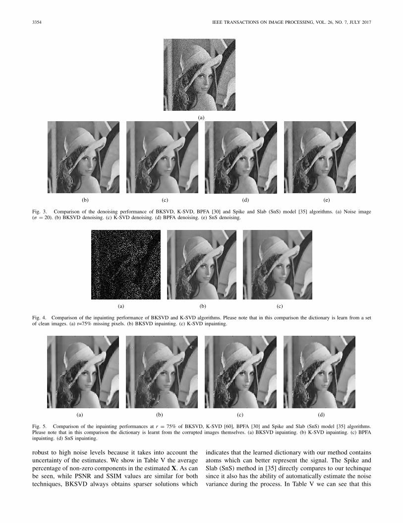
Fig. 3. Comparison of the denoising performance of BKSVD, K-SVD, BPFA [30] and Spike and Slab (SnS) model [35] algorithms. (a) Noise image(σ = 20). (b) BKSVD denoising. (c) K-SVD denoising. (d) BPFA denoising. (e) SnS denoising.

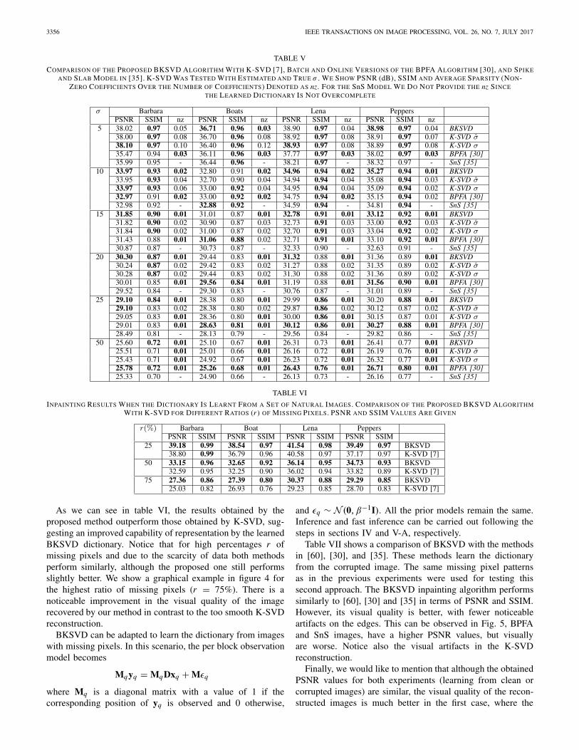
Fig. 4. Comparison of the inpainting performance of BKSVD and K-SVD algorithms. Please note that in this comparison the dictionary is learn from a setof clean images. (a) r=75% missing pixels. (b) BKSVD inpainting. (c) K-SVD inpainting.

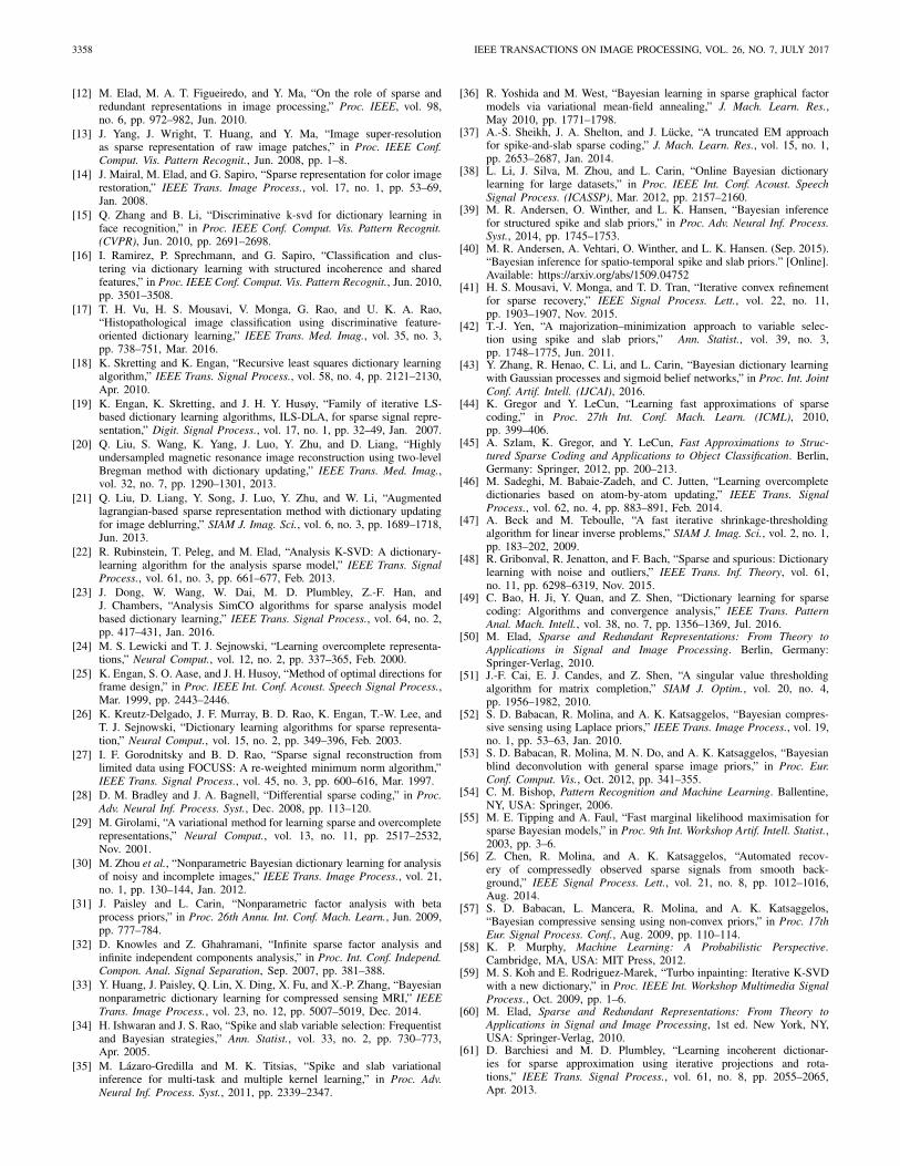
Fig. 5. Comparison of the inpainting performances at r = 75% of BKSVD, K-SVD [60], BPFA [30] and Spike and Slab (SnS) model [35] algorithms.Please note that in this comparison the dictionary is learnt from the corrupted images themselves. (a) BKSVD inpainting. (b) K-SVD inpainting. (c) BPFAinpainting. (d) SnS inpainting.

robust to high noise levels because it takes into account theuncertainty of the estimates. We show in Table V the averagepercentage of non-zero components in the estimated X. As canbe seen, while PSNR and SSIM values are similar for bothtechniques, BKSVD always obtains sparser solutions which

indicates that the learned dictionary with our method containsatoms which can better represent the signal. The Spike andSlab (SnS) method in [35] directly compares to our techinquesince it also has the ability of automatically estimate the noisevariance during the process. In Table V we can see that this


TABLE III

COHERENCE COMPARISON BETWEEN THE PROPOSED TECHNIQUE ANDBPFA [30]. THE DICTIONARIES WERE LEARNED FROM 5e3 PATCHES

OF SIZE 8 × 8 EXTRACTED FROM A SET OF NATURAL IMAGES.DIFFERENT DICTIONARY SIZES K ARE CONSIDERED

TABLE IV

DENOISING PERFORMED ON NOISY Lena USING OMP BY EMPLOYING THEDICTIONARIES LEARNED FROM A SET OF 94e3 PATCHES OF SIZE 8 × 8

EXTRACTED FROM NON-NOISY NATURAL IMAGES. WE SPECIFI-CALLY COMPARE OUR DICTIONARY WITH THE ONE LEARNED

USING THE TECHINQUE IN [30]

method is able to reach competitive results in the denoisingtask. However, our method outperforms SnS in terms of PSNRand SSIM. By comparing the proposed technique with the onein [30] we can see that the two techniques, which both canautomatically estimate the parameters of the model, performalmost equally well. The difference in PSNR and SSIM valuesbetween the two techniques is, in most cases, extremely small.Thus, in order to further assess in detail the differences in thequality of the estimated dictionaries, we rely on the mutualcoherence defined as

μ{D} = maxi �= j

|dᵀi d j |

‖di‖‖d j ‖ .

The mutual coherence provides a measure of the worst sim-ilarity between any two columns in the dictionary; in fact,two columns with high correlation may confuse algorithmsseeking a sparse representation [61]. Even though the designof incoherent dictionary is out of the scope of this work, inTable III we show the mutual coherence of the dictionarieslearned with the proposed technique and the one in [30] tofurther analyze the differences among the two techniques.It can be seen that our technique is able to consistentlyreach lower mutual coherence at different dictionary sizes.We further investigate this aspect by characterizing the qualityof the dictionary itself. In order to perform this task, given a setof non-noisy training patches we learn the dictionaries madeof 256 atoms using both the proposed method and the BPFAtechnique [30]. Then, we use these dictionaries to denoise aspecific image. In order to perform a fair comparison we usethe OMP algorithm for the sparse representation step witha fixed sparsity level s = 3. As can be seen in Table IV,the dictionary learned with the proposed algorithm not onlyhas lower mutual coherence but also shows its ability tobetter sparsely represent a signal by reaching higher PSNRat different noise standard deviations σ .

An example of denoising is shown in Figure 3 wherewe can see the denoised “Lena” provided by the differentmethods we are considering in this section. As shown in thisfigure, the proposed technique preserves edges and high spatialfrequencies better than K-SVD, which produces a flatter and

Fig. 6. Inpainting process: (a) two patches from image I, y1 and yq (missingpixels in red), (b) vectorization of patch yq ; rows from D corresponding tothe missing pixels in yq are also highlighted in red, (c) highlighted entriesare discarded from the problem formulation, (d) recovery using the fulldictionary D.

more blurry image. Moreover, as we already pointed outpreviously, our method does not require any prior informationon the noise corrupting the images since its variance isautomatically estimated. When considering other methods, itcan also be seen that our method is able to generate less visiblehigh-frequency artifacts than BPFA and SnS models.

Table II shows both the true synthetic noise standard devi-ation and the corresponding estimation by our method for thedenoising experiment using the “Lena” image.

B. InpaintingSparse coding is also capable of dealing with missing

information. The problem stated in (1) needs to be adaptedto handle this lack of information at the reconstruction phase,that is, after the dictionary has been learned.

For this experiment, a dictionary of 256 atoms was learnedfrom a database of 23 images. From every image, we selectedthe 4096 patches with the highest variances. Following theapproach in [7], these images did not contain missing values.During testing, and for images not in the training set, 25%,50% and 75% of the pixels in those images were removed(set to zero) from every non-overlapping patch of each 512 ×512 test image. No noise was added. Regarding the K-SVDparameters, a very small σ was used since the image has nonoise.

During testing, the process was adapted to deal with themissing information. Let nq denote the position of the pixelsin a patch q where the information is available. We createthe set of truncated vectors yq = yq(nq ) which contain theentries of yq restricted to the indices in nq , and considerthe set of truncated dictionaries for these signals D(q) =[d1(nq ), · · · , dK (nq)]. We then estimate xq from the obser-vation model

yq = D(q)xq, q = 1, . . . , Q. (73)

Finally, the image is recovered from the estimated repre-sentations xq and the full dictionary, Y = DX. This processis depicted in Figure 6.


TABLE V

COMPARISON OF THE PROPOSED BKSVD ALGORITHM WITH K-SVD [7], BATCH AND ONLINE VERSIONS OF THE BPFA ALGORITHM [30], AND SPIKEAND SLAB MODEL IN [35]. K-SVD WAS TESTED WITH ESTIMATED AND TRUE σ . WE SHOW PSNR (dB), SSIM AND AVERAGE SPARSITY (NON-

ZERO COEFFICIENTS OVER THE NUMBER OF COEFFICIENTS) DENOTED AS nz. FOR THE SnS MODEL WE DO NOT PROVIDE THE nz SINCE

THE LEARNED DICTIONARY IS NOT OVERCOMPLETE

TABLE VI

INPAINTING RESULTS WHEN THE DICTIONARY IS LEARNT FROM A SET OF NATURAL IMAGES. COMPARISON OF THE PROPOSED BKSVD ALGORITHMWITH K-SVD FOR DIFFERENT RATIOS (r ) OF MISSING PIXELS. PSNR AND SSIM VALUES ARE GIVEN

As we can see in table VI, the results obtained by theproposed method outperform those obtained by K-SVD, sug-gesting an improved capability of representation by the learnedBKSVD dictionary. Notice that for high percentages r ofmissing pixels and due to the scarcity of data both methodsperform similarly, although the proposed one still performsslightly better. We show a graphical example in figure 4 forthe highest ratio of missing pixels (r = 75%). There is anoticeable improvement in the visual quality of the imagerecovered by our method in contrast to the too smooth K-SVDreconstruction.

BKSVD can be adapted to learn the dictionary from imageswith missing pixels. In this scenario, the per block observationmodel becomes

Mqyq = MqDxq + Mεq

where Mq is a diagonal matrix with a value of 1 if thecorresponding position of yq is observed and 0 otherwise,

and εq ∼ N (0, β−1I). All the prior models remain the same.Inference and fast inference can be carried out following thesteps in sections IV and V-A, respectively.

Table VII shows a comparison of BKSVD with the methodsin [60], [30], and [35]. These methods learn the dictionaryfrom the corrupted image. The same missing pixel patternsas in the previous experiments were used for testing thissecond approach. The BKSVD inpainting algorithm performssimilarly to [60], [30] and [35] in terms of PSNR and SSIM.However, its visual quality is better, with fewer noticeableartifacts on the edges. This can be observed in Fig. 5, BPFAand SnS images, have a higher PSNR values, but visuallyare worse. Notice also the visual artifacts in the K-SVDreconstruction.

Finally, we would like to mention that although the obtainedPSNR values for both experiments (learning from clean orcorrupted images) are similar, the visual quality of the recon-structed images is much better in the first case, where the


TABLE VII

INPAINTING RESULTS WHEN THE DICTIONARY IS LEARNT FROM THE CORRUPTED IMAGES THEMSELVES. COMPARISON OF THE PROPOSED BKSVDALGORITHM WITH SnS AND BPFA FOR DIFFERENT RATIOS (r ) OF MISSING PIXELS. PSNR AND SSIM VALUES ARE GIVEN

TABLE VIII

RUNTIME IN seconds FOR DICTIONARY LEARNING ALGORITHMS FOR

DIFFERENT IMAGE AND DICTIONARY (K ) SIZES

use of additional clean data improves the construction of thedictionary.

C. Runtime Comparison

We conclude the experimental section with a final compari-son of the dictionary learning algorithms in terms of executiontime. The experiments were performed on a server equippedwith AMD Opteron™CPU @ 2.30 GHz processors. Table VIIIshows runtime for denoising performed on the Lena imagewith σ = 20 for different image and dictionary sizes.

K-SVD is the fastest, but it does not include an estima-tion of the number of non-zeros in each sparse represen-tation. Among the Bayesian methods the proposed methodranks second after BFPA but notice, as pointed out insection V-A, that the proposed method estimates a parameterλkq for every coefficient in the representation matrix, whereasBFPA only estimates one probability vector (K parameters)shared by all xq . It is possible to estimate c such probabilityvectors in BFPA, but this was not used in the experiments.

VII. CONCLUSION

In this paper, we presented a novel Bayesian approachfor the �1 sparse dictionary learning problem based onK-SVD. The prior we utilize on the sparse signals enforcessparsity while allowing for a tractable Bayesian inference.The use of Bayesian modeling and inference allows us to takeinto account the uncertainty of the estimates in the inferenceprocess. Very importantly, the proposed technique estimatesall parameters without the need of any additional information,which makes it fully automatic.

The proposed algorithm has been tested on denoising andinpainting tasks. For the inpainting problem, dictionaries werelearned using two different approaches; first, utilizing a setof clean images, and secondly, from the corrupted imagesthemselves. All evaluated techniques yield good results, but

K-SVD has a major drawback: the need of an accurate estimateof the noise deviation. Bayesian methods solve this deficiency,but at the expense of higher complexity and computationaltime. From the performed experiments, BPFA and the pro-posed method are the best performing ones; notice also thatour method produces images with reduced artifacts. In orderto further characterize the improved quality of our dictionaryestimation, we evaluated it in terms of lower mutual coherenceand better image recovery under common sparse presentationalgorithms.

Lastly, experiments to analyze the importance of the dictio-nary size have been carried out. These experiments can be usedto tune the size of the dictionary. We have not addressed herethe estimation of the size of the dictionary using Bayesianinference. However, we are currently investigating how toadapt to our model the approach to initially estimate thedictionary size presented in [30].

REFERENCES

[1] R. G. Baraniuk and M. B. Wakin, “Random projections of smoothmanifolds,” Found. Comput. Math., vol. 9, no. 1, pp. 51–77, Feb. 2009.

[2] A. Eftekhari and M. B. Wakin, New Analysis of Manifold Embeddingsand Signal Recovery From Compressive Measurements. New York, NY,USA: Elsevier, 2013.

[3] R. Rubinstein, A. M. Bruckstein, and M. Elad, “Dictionaries for sparserepresentation modeling,” Proc. IEEE, vol. 98, no. 6, pp. 1045–1057,Jun. 2010.

[4] E. P. Simoncelli, W. T. Freeman, E. H. Adelson, and D. J. Heeger,“Shiftable multiscale transforms,” IEEE Trans. Inf. Theory, vol. 38,no. 2, pp. 587–607, Mar. 1992.

[5] B. A. Olshausen and D. J. Field, “Emergence of simple-cell receptivefield properties by learning a sparse code for natural images,” Nature,vol. 381, no. 6583, pp. 607–609, Jun. 1996.

[6] B. A. Olshausen and D. J. Field, “Sparse coding with an overcompletebasis set: A strategy employed by V1?” Vis. Res., vol. 37, no. 23,pp. 3311–3325, 1997.

[7] M. Aharon, M. Elad, and A. Bruckstein, “K-SVD: An algorithm fordesigning overcomplete dictionaries for sparse representation,” IEEETrans. Signal Process., vol. 54, no. 11, pp. 4311–4322, Nov. 2006.

[8] J. Mairal, F. Bach, J. Ponce, and G. Sapiro, “Online dictionary learningfor sparse coding,” in Proc. 26th Annu. Int. Conf. Mach. Learn.,Jun. 2009, pp. 689–696.

[9] M. Zhou et al., “Nonparametric Bayesian dictionary learning for analysisof noisy and incomplete images,” IEEE Trans. Image Process., vol. 21,no. 1, pp. 130–144, Jan. 2012.

[10] J. Shi, X. Ren, G. Dai, J. Wang, and Z. Zhang, “A non-convex relaxationapproach to sparse dictionary learning,” in Proc. IEEE Conf. Comput.Vis. Pattern Recognit. (CVPR), Jun. 2011, pp. 1809–1816.

[11] M. Elad and M. Aharon, “Image denoising via sparse and redundantrepresentations over learned dictionaries,” IEEE Trans. Image Process.,vol. 15, no. 12, pp. 3736–3745, Dec. 2006.


[12] M. Elad, M. A. T. Figueiredo, and Y. Ma, “On the role of sparse andredundant representations in image processing,” Proc. IEEE, vol. 98,no. 6, pp. 972–982, Jun. 2010.

[13] J. Yang, J. Wright, T. Huang, and Y. Ma, “Image super-resolutionas sparse representation of raw image patches,” in Proc. IEEE Conf.Comput. Vis. Pattern Recognit., Jun. 2008, pp. 1–8.

[14] J. Mairal, M. Elad, and G. Sapiro, “Sparse representation for color imagerestoration,” IEEE Trans. Image Process., vol. 17, no. 1, pp. 53–69,Jan. 2008.

[15] Q. Zhang and B. Li, “Discriminative k-svd for dictionary learning inface recognition,” in Proc. IEEE Conf. Comput. Vis. Pattern Recognit.(CVPR), Jun. 2010, pp. 2691–2698.

[16] I. Ramirez, P. Sprechmann, and G. Sapiro, “Classification and clus-tering via dictionary learning with structured incoherence and sharedfeatures,” in Proc. IEEE Conf. Comput. Vis. Pattern Recognit., Jun. 2010,pp. 3501–3508.

[17] T. H. Vu, H. S. Mousavi, V. Monga, G. Rao, and U. K. A. Rao,“Histopathological image classification using discriminative feature-oriented dictionary learning,” IEEE Trans. Med. Imag., vol. 35, no. 3,pp. 738–751, Mar. 2016.

[18] K. Skretting and K. Engan, “Recursive least squares dictionary learningalgorithm,” IEEE Trans. Signal Process., vol. 58, no. 4, pp. 2121–2130,Apr. 2010.

[19] K. Engan, K. Skretting, and J. H. Y. Husøy, “Family of iterative LS-based dictionary learning algorithms, ILS-DLA, for sparse signal repre-sentation,” Digit. Signal Process., vol. 17, no. 1, pp. 32–49, Jan. 2007.

[20] Q. Liu, S. Wang, K. Yang, J. Luo, Y. Zhu, and D. Liang, “Highlyundersampled magnetic resonance image reconstruction using two-levelBregman method with dictionary updating,” IEEE Trans. Med. Imag.,vol. 32, no. 7, pp. 1290–1301, 2013.

[21] Q. Liu, D. Liang, Y. Song, J. Luo, Y. Zhu, and W. Li, “Augmentedlagrangian-based sparse representation method with dictionary updatingfor image deblurring,” SIAM J. Imag. Sci., vol. 6, no. 3, pp. 1689–1718,Jun. 2013.

[22] R. Rubinstein, T. Peleg, and M. Elad, “Analysis K-SVD: A dictionary-learning algorithm for the analysis sparse model,” IEEE Trans. SignalProcess., vol. 61, no. 3, pp. 661–677, Feb. 2013.

[23] J. Dong, W. Wang, W. Dai, M. D. Plumbley, Z.-F. Han, andJ. Chambers, “Analysis SimCO algorithms for sparse analysis modelbased dictionary learning,” IEEE Trans. Signal Process., vol. 64, no. 2,pp. 417–431, Jan. 2016.

[24] M. S. Lewicki and T. J. Sejnowski, “Learning overcomplete representa-tions,” Neural Comput., vol. 12, no. 2, pp. 337–365, Feb. 2000.

[25] K. Engan, S. O. Aase, and J. H. Husoy, “Method of optimal directions forframe design,” in Proc. IEEE Int. Conf. Acoust. Speech Signal Process.,Mar. 1999, pp. 2443–2446.

[26] K. Kreutz-Delgado, J. F. Murray, B. D. Rao, K. Engan, T.-W. Lee, andT. J. Sejnowski, “Dictionary learning algorithms for sparse representa-tion,” Neural Comput., vol. 15, no. 2, pp. 349–396, Feb. 2003.

[27] I. F. Gorodnitsky and B. D. Rao, “Sparse signal reconstruction fromlimited data using FOCUSS: A re-weighted minimum norm algorithm,”IEEE Trans. Signal Process., vol. 45, no. 3, pp. 600–616, Mar. 1997.

[28] D. M. Bradley and J. A. Bagnell, “Differential sparse coding,” in Proc.Adv. Neural Inf. Process. Syst., Dec. 2008, pp. 113–120.

[29] M. Girolami, “A variational method for learning sparse and overcompleterepresentations,” Neural Comput., vol. 13, no. 11, pp. 2517–2532,Nov. 2001.

[30] M. Zhou et al., “Nonparametric Bayesian dictionary learning for analysisof noisy and incomplete images,” IEEE Trans. Image Process., vol. 21,no. 1, pp. 130–144, Jan. 2012.

[31] J. Paisley and L. Carin, “Nonparametric factor analysis with betaprocess priors,” in Proc. 26th Annu. Int. Conf. Mach. Learn., Jun. 2009,pp. 777–784.

[32] D. Knowles and Z. Ghahramani, “Infinite sparse factor analysis andinfinite independent components analysis,” in Proc. Int. Conf. Independ.Compon. Anal. Signal Separation, Sep. 2007, pp. 381–388.

[33] Y. Huang, J. Paisley, Q. Lin, X. Ding, X. Fu, and X.-P. Zhang, “Bayesiannonparametric dictionary learning for compressed sensing MRI,” IEEETrans. Image Process., vol. 23, no. 12, pp. 5007–5019, Dec. 2014.

[34] H. Ishwaran and J. S. Rao, “Spike and slab variable selection: Frequentistand Bayesian strategies,” Ann. Statist., vol. 33, no. 2, pp. 730–773,Apr. 2005.

[35] M. Lázaro-Gredilla and M. K. Titsias, “Spike and slab variationalinference for multi-task and multiple kernel learning,” in Proc. Adv.Neural Inf. Process. Syst., 2011, pp. 2339–2347.

[36] R. Yoshida and M. West, “Bayesian learning in sparse graphical factormodels via variational mean-field annealing,” J. Mach. Learn. Res.,May 2010, pp. 1771–1798.

[37] A.-S. Sheikh, J. A. Shelton, and J. Lücke, “A truncated EM approachfor spike-and-slab sparse coding,” J. Mach. Learn. Res., vol. 15, no. 1,pp. 2653–2687, Jan. 2014.

[38] L. Li, J. Silva, M. Zhou, and L. Carin, “Online Bayesian dictionarylearning for large datasets,” in Proc. IEEE Int. Conf. Acoust. SpeechSignal Process. (ICASSP), Mar. 2012, pp. 2157–2160.

[39] M. R. Andersen, O. Winther, and L. K. Hansen, “Bayesian inferencefor structured spike and slab priors,” in Proc. Adv. Neural Inf. Process.Syst., 2014, pp. 1745–1753.

[40] M. R. Andersen, A. Vehtari, O. Winther, and L. K. Hansen. (Sep. 2015).“Bayesian inference for spatio-temporal spike and slab priors.” [Online].Available: https://arxiv.org/abs/1509.04752

[41] H. S. Mousavi, V. Monga, and T. D. Tran, “Iterative convex refinementfor sparse recovery,” IEEE Signal Process. Lett., vol. 22, no. 11,pp. 1903–1907, Nov. 2015.

[42] T.-J. Yen, “A majorization–minimization approach to variable selec-tion using spike and slab priors,” Ann. Statist., vol. 39, no. 3,pp. 1748–1775, Jun. 2011.

[43] Y. Zhang, R. Henao, C. Li, and L. Carin, “Bayesian dictionary learningwith Gaussian processes and sigmoid belief networks,” in Proc. Int. JointConf. Artif. Intell. (IJCAI), 2016.

[44] K. Gregor and Y. LeCun, “Learning fast approximations of sparsecoding,” in Proc. 27th Int. Conf. Mach. Learn. (ICML), 2010,pp. 399–406.

[45] A. Szlam, K. Gregor, and Y. LeCun, Fast Approximations to Struc-tured Sparse Coding and Applications to Object Classification. Berlin,Germany: Springer, 2012, pp. 200–213.

[46] M. Sadeghi, M. Babaie-Zadeh, and C. Jutten, “Learning overcompletedictionaries based on atom-by-atom updating,” IEEE Trans. SignalProcess., vol. 62, no. 4, pp. 883–891, Feb. 2014.

[47] A. Beck and M. Teboulle, “A fast iterative shrinkage-thresholdingalgorithm for linear inverse problems,” SIAM J. Imag. Sci., vol. 2, no. 1,pp. 183–202, 2009.

[48] R. Gribonval, R. Jenatton, and F. Bach, “Sparse and spurious: Dictionarylearning with noise and outliers,” IEEE Trans. Inf. Theory, vol. 61,no. 11, pp. 6298–6319, Nov. 2015.

[49] C. Bao, H. Ji, Y. Quan, and Z. Shen, “Dictionary learning for sparsecoding: Algorithms and convergence analysis,” IEEE Trans. PatternAnal. Mach. Intell., vol. 38, no. 7, pp. 1356–1369, Jul. 2016.

[50] M. Elad, Sparse and Redundant Representations: From Theory toApplications in Signal and Image Processing. Berlin, Germany:Springer-Verlag, 2010.

[51] J.-F. Cai, E. J. Candes, and Z. Shen, “A singular value thresholdingalgorithm for matrix completion,” SIAM J. Optim., vol. 20, no. 4,pp. 1956–1982, 2010.

[52] S. D. Babacan, R. Molina, and A. K. Katsaggelos, “Bayesian compres-sive sensing using Laplace priors,” IEEE Trans. Image Process., vol. 19,no. 1, pp. 53–63, Jan. 2010.

[53] S. D. Babacan, R. Molina, M. N. Do, and A. K. Katsaggelos, “Bayesianblind deconvolution with general sparse image priors,” in Proc. Eur.Conf. Comput. Vis., Oct. 2012, pp. 341–355.

[54] C. M. Bishop, Pattern Recognition and Machine Learning. Ballentine,NY, USA: Springer, 2006.

[55] M. E. Tipping and A. Faul, “Fast marginal likelihood maximisation forsparse Bayesian models,” in Proc. 9th Int. Workshop Artif. Intell. Statist.,2003, pp. 3–6.

[56] Z. Chen, R. Molina, and A. K. Katsaggelos, “Automated recov-ery of compressedly observed sparse signals from smooth back-ground,” IEEE Signal Process. Lett., vol. 21, no. 8, pp. 1012–1016,Aug. 2014.

[57] S. D. Babacan, L. Mancera, R. Molina, and A. K. Katsaggelos,“Bayesian compressive sensing using non-convex priors,” in Proc. 17thEur. Signal Process. Conf., Aug. 2009, pp. 110–114.

[58] K. P. Murphy, Machine Learning: A Probabilistic Perspective.Cambridge, MA, USA: MIT Press, 2012.

[59] M. S. Koh and E. Rodriguez-Marek, “Turbo inpainting: Iterative K-SVDwith a new dictionary,” in Proc. IEEE Int. Workshop Multimedia SignalProcess., Oct. 2009, pp. 1–6.

[60] M. Elad, Sparse and Redundant Representations: From Theory toApplications in Signal and Image Processing, 1st ed. New York, NY,USA: Springer-Verlag, 2010.

[61] D. Barchiesi and M. D. Plumbley, “Learning incoherent dictionar-ies for sparse approximation using iterative projections and rota-tions,” IEEE Trans. Signal Process., vol. 61, no. 8, pp. 2055–2065,Apr. 2013.


Juan G. Serra received the degree in telecommuni-cations engineering from the Universitat Politècnicade Valéncia in 2014 and the M.S. degree in data sci-ence and computer engineering from the Universityof Granada in 2016, where he is currently pursuingthe Ph.D. degree, under the supervision of Prof.Molina, being a member of the Visual InformationProcessing Group, Department of Computer Scienceand Artificial Intelligence. His research interestsfocus on the use of Bayesian modeling and inferenceto solve different inverse problems related to dictio-

nary learning, image restoration and machine learning. During his research,he has addressed several problems, such as blind image deconvolution, imagedenoising, and inpainting and multispectral image classification.

Matteo Testa received the B.Sc. degree and theM.Sc. degree in telecommunications engineeringfrom the Politecnico di Torino, Turin, Italy, in 2011and 2012, respectively, and the Ph.D. degree inelectronic and communications engineering fromthe Electronics Department, Politecnico di Torino,in 2016, under the supervision of Prof. E. Magli.He currently holds a post-doctoral position with theIPL laboratory, Politecnico di Torino, led by Prof.E. Magli in collaboration with SONY EuTEC. Hisresearch is focused on compressed sensing with a

particular interest on imaging systems, forensic applications, and Bayesianinference.

Rafael Molina was born in 1957. He received thedegree in mathematics (statistics) and the Ph.D.degree in optimal design in linear models from theUniversity of Granada, Granada, Spain, in 1979 and1983, respectively. He was a Professor of ComputerScience and Artificial Intelligence with the Univer-sity of Granada, Granada, Spain, in 2000. He wasthe Dean of the Computer Engineering School, theUniversity of Granada, from 1992 to 2002, where hewas the Head of the Computer Science and ArtificialIntelligence Department from 2005 to 2007. His

research interest focuses mainly on using Bayesian modeling and inference inproblems, such as image restoration (applications to astronomy and medicine),superresolution of images and video, blind deconvolution, computationalphotography, source recovery in medicine, compressive sensing, low-rankmatrix decomposition, active learning, fusion, and classification.

Dr. Molina is a recipient of the IEEE International Conference on ImageProcessing Paper Award in 2007 and the ISPA Best Paper Award in 2009.He is a co-author of a paper awarded the runner-up prize at Reception forearly-stage researchers at the House of Commons. He serves as an AssociateEditor of Applied Signal Processing from 2005 to 2007, and also has beenan Associate Editor of the IEEE TRANSACTIONS ON IMAGE PROCESSING

since 2010, and the Progress in Artificial Intelligence since 2011, and an AreaEditor of the Digital Signal Processing since 2011.

Aggelos K. Katsaggelos (F’98) received theDiploma degree in electrical and mechanical engi-neering from the Aristotelian University of Thes-saloniki, Greece, in 1979, and the M.S. and Ph.D.degrees in electrical engineering from the GeorgiaInstitute of Technology, in 1981 and 1985, respec-tively. He was the holder of the Ameritech Chairof Information Technology and the AT&T Chairand the Co-Founder and Director of the MotorolaCenter for Seamless Communications. In 1985, hejoined the Department of Electrical Engineering and

Computer Science, Northwestern University, where he is currently a Professor,holder of the Joseph Cummings Chair. He is a member of the AcademicStaff, NorthShore University Health System, a Faculty Member with theDepartment of Linguistics, and he has an appointment with the ArgonneNational Laboratory. He has authored extensively in the areas of multimediaprocessing and communications (over 250 journal papers, 500 conferencepapers and 40 book chapters) and he is the holder of 26 international patents.He has co-authored of the book Rate-Distortion Based Video Compression(Kluwer, 1997), the Super-Resolution for Images and Video (Claypool, 2007),the Joint Source-Channel Video Transmission (Claypool, 2007), the MachineLearning Refined (Cambridge University Press, 2016), and The Essentialsof Sparse Modeling and Optimization (Springer, 2017, forthcoming). He hassupervised 56 Ph.D. dissertations so far.

Prof. Katsaggelos was the Editor-in-Chief of the IEEE Signal ProcessingMagazine from 1997 to 2002, a BOG Member of the IEEE Signal ProcessingSociety from 1999 to 2001, a member of the Publication Board of theIEEE Proceedings from 2003 to 2007. He is currently a member of theAwards Board of the Signal Processing Society. He is a fellow of the SPIEin 2009. He is a recipient of the IEEE Third Millennium Medal in 2000,the IEEE Signal Processing Society Meritorious Service Award in 2001, theIEEE Signal Processing Society Technical Achievement Award in 2010,the IEEE Signal Processing Society Best Paper Award in 2001, the IEEEICME Paper Award in 200), the IEEE ICIP Paper Award in 2007, the ISPAPaper Award in 2009, and the EUSIPCO Paper Award in 2013. He was aDistinguished Lecturer of the IEEE Signal Processing Society from 2007 to2008.

Documents

3344 IEEE TRANSACTIONS ON IMAGE PROCESSING, VOL. 26, NO. …decsai.ugr.es/vip/files/journals/07875464.pdf · 3344 IEEE TRANSACTIONS ON IMAGE PROCESSING, VOL. 26, NO. 7, JULY 2017