http://hdl.handle.net/10552/3301

Abbas, A., Syed Mohsin, S. and Cotsovos, D. (2013), ‘Seismic response of steel fibre reinforced concrete beam-column joints’, Engineering Structures, [In press], doi: 10.1016/j.engstruct.2013.10.046 This is the Accepted Version of this work. Copyright statement: NOTICE: this is the author’s version of a work that was accepted for publication in Engineering Structures. Changes resulting from the publishing process, such as peer review, editing, corrections, structural formatting, and other quality control mechanisms may not be reflected in this document. Changes may have been made to this work since it was submitted for publication. A definitive version will be published in Engineering Structures with the DOI:10.1016/j.engstruct.2013.10.046 DOI for the version of record: 10.1016/j.engstruct.2013.10.046

Licence for this version: Creative Commons Attribution-NonCommercial-NoDerivs

This work was downloaded from roar.uel.ac.uk UEL Research Open Access Repository

1

SEISMIC RESPONSE OF STEEL FIBRE REINFORCED CONCRETE BEAM-COLUMN

JOINTS

* Ali A. Abbas BSc(Eng.), DIC, PhD, FHEA School of Architecture, Computing and Engineering, University of East London,

London E16 2RD, UK Tel.: 020 8223 6279, Fax: 020 8223 2963

E-mail: abbas@uel.ac.uk

Sharifah M. Syed Mohsin BSc(Eng.), DIC, PhD Department of Civil and Environmental Engineering, Imperial College London,

London SW7 2BU, UK E-mail: s.syed-mohsin08@imperial.ac.uk

Demetrios M. Cotsovos Dipl Ing, MSc, DIC, PhD, CEng Institute of Infrastructure and Environment, School of the Built Environment, Heriot-Watt

University, Edinburgh, EH14 4AS, UK E-mail: d.cotsovos@hw.ac.uk

* Corresponding Author.

2

ABSTRACT

The present research work aims to investigate numerically the behaviour of steel fibre

reinforced concrete beam-column joints under seismic action. Both exterior and interior joint

types were examined and 3D nonlinear finite element analyses were carried out using

ABAQUS software. The joints were subjected to reversed-cyclic loading, combined with a

constant axial force on the column representing gravity loads. The joints were initially

calibrated using existing experimental data – to ascertain the validity of the numerical model

used – and then parametric studies were carried out using different steel fibre ratios coupled

with increased spacing of shear links. The aim was to assess the effect of introducing steel

fibres into the concrete mix in order to compensate for a reduced amount of conventional

transverse steel reinforcement and hence lessen congestion of the latter. This is particularly

useful for joints designed to withstand seismic loading as code requirements (e.g. Eurocode

8) lead to a high amount of shear links provided to protect critical regions. The spacing

between shear links was increased by 0%, 50% and 100%, whilst the fibre volume fraction (Vf)

was increased by 0%, 1%, 1.5%, 2% and 2.5%. Potential enhancement to ductility, a key

requirement in seismic design, was investigated as well as potential improvements to energy

absorption and confinement. The work also examined key structural issues such as strength,

storey drift, plastic hinges formation and cracking patterns.

Keywords: steel fibres; beam-column joints; finite-element analysis; reinforced concrete;

cracking; seismic design; structural failure; nonlinear behaviour

3

1. INTRODUCTION

The structural analysis of frames is commonly based on the assumption that the joints

formed at the beam-column intersections behave as rigid bodies. However, published

experimental data [1-8] and numerical studies [9] reveal that for the case of reinforced-

concrete (RC) structures, the “rigid joint” assumption is rather crude since cracks may form

within the joint region early in the loading process. The behaviour of the RC joints departs

even more form the rigid-joint assumption when considering the slippage of reinforcement,

which may sometimes play an important role in the response of joints, especially with

insufficient anchorage reinforcement length [10, 11]. As a result, the displacements and

rotations transferred through each joint to the ends of the adjoining beams and columns can

be significantly affected by the cracking and the ensuing deformation of the joint itself. This,

in turn, may have a significant impact on the distribution of the internal actions developing

along the structural elements of the frame affecting the overall structural performance.

Although, current codes of practice for earthquake-resistant design require structures to

comply with specific performance requirements, the effect of crack-formation within the

joint region is essentially ignored during the structural analysis phase of RC frame structures.

In order to safeguard against brittle types of failure and to enhance ductility and load-

carrying capacity, current codes of practice, e.g. Eurocode 2 [12] and Eurocode 8 [13],

dictate the use of dense arrangements of shear links especially in the critical regions of RC

frames (i.e. beams, columns and within the joints). Nevertheless, this can result in

reinforcement congestion which causes difficulties during concreting (i.e. incomplete

compaction of concrete) and increases construction costs. Furthermore, published test data

[1-8] and in particular the two studies by Tsonos [5, 6] demonstrated that design codes’

provisions [12, 13] did not safeguard against premature joint shear failure because the

resulting design cannot ensure that the joint shear stress will be significantly lower than the

joint ultimate strength in order to ascertain the development of the optimal (ductile) failure

mechanism with plastic hinges forming in the beams while columns remained essentially

elastic, to conform to the requisite “strong column-weak beam” tenet of capacity design. An

improved model was also proposed in order to ensure that beam-column joints are kept

intact during strong earthquakes [6].

The present research work was carried out to examine numerically the potential benefits

stemming from the introduction of steel fibres into the concrete mix on the nonlinear

4

behaviour of RC beam-column joint assemblages under seismic action. The aim is to

investigate whether the use of steel fibres can (i) improve the structural performance of the

joint, (ii) enhance the overall structural response of the RC structural configurations

presently studied and (iii) lead to a substantial reduction of conventional steel reinforcement

(particularly shear links). The nonlinear analysis of the responses of the RC structural

configurations investigated is based on the use of the well-known commercial finite element

software package ABAQUS [14]. The programme is capable of carrying out three-

dimensional (3D) static and dynamic nonlinear finite element analysis (NLFEA) and

incorporates material models describing the nonlinear behaviour of plain concrete. The

latter was modified in order to introduce the effect of steel fibres particularly on the

cracking processes concrete undergoes when subjected to external loading. Based on initial

phase of the present work [15-17], the adopted model was found to be capable of providing

realistic predictions concerning the response of conventionally reinforced and steel fibre

reinforced concrete (SFRC) beams under both monotonic and cyclic loading. The attention of

the numerical investigation was initially focused on validating the predictions obtained for

the nonlinear behaviour of SFRC beam-column joints selected for this study [4,18]. At the

same time the present investigation also aims at assessing how certain important aspects of

structural response (i.e. stiffness, load-carrying capacity, deformation profile, cracking,

ductility and mode of failure) are affected by the presence of the steel fibres within the

concrete medium. For this purpose two types of beam-column joint assemblages are

considered herein, namely: an external (T-shape) and a series of internal (Cross-shape)

joints. The behaviour of these specimens was studied experimentally in the past by

Filiatrault et al. [4] and Bayasi and Gebman [18]. The joints were subjected to reversed-cyclic

loading, which is the key feature of seismic action, combined with a constant axial force on

the column representing gravity loads.

Following the validation of the numerical predictions, a parametric investigation was carried

out aiming at assessing the extent to which the enhancement of concrete material

properties (through the use of steel fibres) can improve the structural performance of the RC

beam-column joints mentioned earlier at both the serviceability and ultimate limit states.

Furthermore, the present investigation examined whether the use of steel fibres can result

in a substantial reduction of conventional transverse reinforcement without compromising

ductility and strength requirements set by the current design codes [12,13]. The parameters

considered herein are the fibre volume fraction (Vf) and the spacing increase (SI) between

5

the shear links. The spacing between shear links was increased while steel fibres were added

as a substitute (so the spacing between shear links was increased by 0%, 50% and 100%,

while the fibre volume fraction (Vf) was increased by 0%, 1%, 1.5%, 2% and 2.5%). In this

manner, overall conclusions were made on the potential of fibres to compensate for

reduction in conventional transverse reinforcement.

2. FE MODELLING OF SFRC BEHAVIOUR

The effect of steel fibres on the behaviour of structural concrete at the material level has

been investigated experimentally in the past by many researchers and an extended

literature review on the subject is provided by Syed Mohsin [15]. SFRC prism specimens have

been tested in compression, tension (either under direct tension or splitting) and bending.

Based on the available test data, the introduction of steel-fibres into the concrete mix

predominantly results in an enhancement to the tensile post-cracking behaviour exhibited

after crack formation, allowing concrete to exhibit more ductile characteristics compared to

the fully brittle behaviour exhibited by plain concrete specimens [19]. However, this

profound improvement is not observed in the case of uniaxial compression. This suggests

that the fibres within the concrete mix act primarily in tension, prohibiting the formation

and extension of cracking, whereas in compression one could conservatively assume that

their effect on the concrete strength could be ignored.

Depending on the amount and type of fibres used, the post-cracking behaviour is either

described by a strain softening or hardening stress-strain branch. The residual strength

exhibited after the onset of cracking is the result of the steel-fibres bridging the crack and

the bond developing between the fibre and the surrounding concrete on either side of the

crack. The use of small fibre contents normally results in a softening post-cracking response

as the first cracking strength is the ultimate strength and further deformation is governed by

the opening of a single crack. On the other hand, the addition of higher values of fibre

content can result in a strain-hardening response as the fibres are able to sustain more load

after the formation of the first crack and consequently more cracks will be formed (thus, this

type of behaviour is associated with the formation of multiple cracks). The amount of crack

opening affects the shear behaviour. Usually in the non-linear FE analysis of reinforced-

concrete structures “shear retention” is used to allow for the effect of aggregate interlock

and dowel action. Fibres provide a similar effect on shear response (i.e. in a direction parallel

6

to the crack) and, therefore, it was modelled using the “shear retention” part of ABAQUS

[14] concrete model. The shear stiffness of the concrete decreases when crack is

propagated. Therefore, in order to allow for degradation in shear stiffness due to crack

propagation, the shear modulus was reduced in a linear fashion from full shear retention

(i.e. no degradation) at the cracking strain to 50% of that value at the ultimate tensile strain.

The “brittle cracking model” in ABAQUS [14] was adopted for the present work. The model

is designed for cases in which the material behaviour is dominated by tensile cracking as is

normally the case for structural concrete. To make the numerical solution even more

efficient, the analysis is usually carried out using the dynamic solver as a quasi-static one (i.e.

with a low rate of loading). Therefore in the present study, “brittle cracking model” was used

in conjunction with the explicit dynamic procedure available in ABAQUS/Explicit. This was

one of the practical reasons for selecting the model for the present investigations of SFRC

behaviour under reversed-cyclic loading. Moreover, the model was successfully used to

predict the responses of different SFRC forms such as simply-supported beams, statically-

indeterminate elements as well as the present study of joints. The studies have shown that

the model is capable of predicting both brittle (i.e. shear) and ductile (i.e. bending) forms of

failure, as described fully elsewhere [15, 16, 17].

A number of available constitutive models for SFRC have been identified such as those

proposed by RILEM [20,21], Barros [22,23], Tlemat et al. [24], Lok and Pei [25] and Lok and

Xiao [26]. The constitutive relations have been developed to describe the uniaxial tensile

stress-strain relationship of SFRC (in particular the post-cracking behaviour of SFRC allowing

the latter to exhibit more ductile characteristics compared to the brittle response of plain

concrete [19]). In these models, the residual strength beyond the cracking point of concrete

is made up of two components, the steel fibres bridging the crack and the bond developing

between the fibre and the surrounding concrete (leading eventually to pull-out failure when

such bond is lost under increased loading). The main characteristics of the models were

closely studied and a calibration study was undertaken by Syed Mohsin [15] and Abbas et al.

[16,17] using NLFEA to examine these models and it was found that the use of Lok and Xiao

model [26] to simulate SFRC material behaviour in tension resulted in realistic predictions

concerning the response of a wide range of structural forms. Consequently, this model was

selected for the subsequent parametric studies. In the model, the post-cracking behaviour of

SFRC is described by the tension softening (and in some cases hardening) portion of the

7

stress-strain curve exhibited after crack formation, which is dependent on the fibre content

as well as the shape and size of the fibres. The stress-strain relationships describing the

behaviour of SFRC under uniaxial tension are:

= ft [2(ε/ εto) – ( ε/ εto)2] for (0 ≤ε ≤ εto)

= ft [1– (1- ftu /ft)( ε–εto / εt1–εto)] for (εto ≤ ε ≤ εt1) (1)

= ftu for (εt1 ≤ ε ≤ εtu)

where ft , ftu are the ultimate and residual tensile strengths of SFRC whereas , εto and εt1 are

the corresponding strains defined as [25]:

ftu = η.Vf .τd.L/d , εt1 = τd .L/d.1/ES (2)

where η is the fibre orientation factor that takes account of the 3 dimensional (3D) random

distribution of fibres, which takes values between 0.405 to 0.5 [26]. In addition, Vf is the

fibre volume fraction, τd is the bond stress between concrete and steel fibres, L/d is the

aspect ratio of the steel fibre and Es is the modulus of elasticity of steel fibres.

The cracking process that concrete undergoes is modelled by employing the smeared crack

approach. A crack forms when the predicted value of stress developing in a given part of the

structure corresponds to a point in the principal stress space that lies outside the surface

defining the failure criterion for concrete, thus resulting in localised material failure. The

plane of the crack is normal to the direction in which the largest principal tensile stress acts.

For purposes of crack detection, a simple Rankine failure criterion is used to detect crack

initiation (i.e. a crack forms when the maximum principal tensile stress attains the specified

tensile strength of concrete). The concrete medium is modelled by using a dense mesh of 8-

node brick elements; the element formulation adopts a reduced integration scheme. The

concrete model adopts fixed, orthogonal cracks, with the maximum number of cracks at a

material point limited by the number of direct stress components present at that material

(Gauss) point of the finite element model (a maximum of three cracks in three-dimensional).

Allowance is made for crack closure, which is important in simulating cyclic loading. An

iterative procedure based on the well-established Newton-Raphson method is used in order

to account for the stress redistributions during which the crack formation and closure checks

as well as convergence checks are carried out. The iterations are repeated until the residual

forces attain a predefined minimum value (i.e. convergence criteria).

8

In the present study, the steel properties for longitudinal bars and shear links were modelled

using a standard elastic-plastic material model. The stress-strain relation adopted is the one

recommended in Eurocode 2 [12], which employs isotropic hardening in which the yields

stress increases as plastic straining occurs. An ultimate tensile strain was also defined to

detect any failure on the steel main bars or stirrups. The reinforcement bars (both

longitudinal and transverse) were simply modelled as 1D truss elements, which is realistic

since they have no practical flexural stiffness.

3. STRUCTURAL FORMS INVESTIGATED

Two types of beam-column joint assemblages were considered in the present investigation,

an external (T-shape) and a series of internal (Cross-shape) joints. The response of the

external joints was established experimentally by Bayasi and Gebman [18] whereas the

response of the internal joints was established by Filiatrault et al. [4].

3.1. External joints specimens

The geometry and reinforcement arrangements for the external beam-column joint [18] are

presented in Fig. 1. Hooked-end steel fibres, 30 mm in length, 0.5 mm in diameter were

added to the concrete mix in order to achieve a fibre content of Vf = 2% (expressed as a

volume fraction ). The hoops (i.e. stirrups) spacing considered is 152 mm centre-to-centre

uniformly applied throughout the beam and column. The uniaxial compressive (fc) and

tensile (ft) strength of concrete was 23.9MPa and 2.4MPa, respectively. The yield stress (fy)

and the modulus of elasticity (Es) of both the longitudinal and transverse reinforcement bars

was 420 MPa and 206 GPa, respectively. The stress-strain diagram describing the behaviour

of SFRC in uniaxial tension is depicted in Fig. 2a. The stress-stain curve describing the

behaviour of the (longitudinal and transverse) reinforcement bars in tension and

compression is shown in Fig. 2b. During testing the top and bottom of the column were

restrained so as to form hinges and reversed-cyclic loading was applied vertically in the form

of a concentrated displacement load near the free-end of the cantilever beam (see Fig. 1).

The loading history input data adopted in this case study is shown in Fig. 3. Steel plates of 20

mm thickness were added at the support for the whole surface area of the column, and at

loading point region along the beam width (this is to mimic experimental conditions and also

avoid development of stress concentrations and premature localised failure in the FE

simulation).

9

3.2. Internal joint specimens

The geometry and reinforcement details of the three full-scale internal beam-column joints

(specimens S1, S2 and S3) tested by Filiatrault et al. [4] are presented in Fig.4. The specimens

were arranged to have the same the longitudinal reinforcement in the beam and column and

to differ only in the transverse (i.e. shear links) arrangements. The idea was that one

specimen would have full conventional seismic shear reinforcement, while the other two

would have reduced conventional reinforcement with fibres being added as a replacement

in one specimen and with no fibres in the other. Therefore, one of the joints specimens S2

(see Fig. 4b) was designed with seismic detailing in accordance to the National Building Code

of Canada [27] and thus was provided with a dense arrangement of (double) shear links. This

is similar to the seismic detailing required to protect the critical regions recommended by

the European codes [13].

The other two joint specimens S1 and S3 (shown in Fig. 4a) were provided with less shear

links than S2 and therefore do not satisfy the code seismic provisions. No steel fibres were

used for specimen S1, whereas in the case of specimen S3 hooked-end steel fibres were

introduced in the critical region around the joint with Vf = 1.6% (i.e. the SFRC zone on

specimen S3 covers the range occupied by the closely-spaced shear links in Figure 4b). Thus

joint S1 represents the specimen with deficient seismic reinforcement, while S3 represents

the SFRC joint with fibres added to compensate for the reduced conventional seismic

reinforcement. The hooked-end steel fibres had a length of 50 mm and a diameter of 0.5

mm. The compressive strength fc and elasticity modulus Ec of plain concrete as well as the

yield strength fy of the steel reinforcement bars was 46 MPa, 35GPa and 400 MPa,

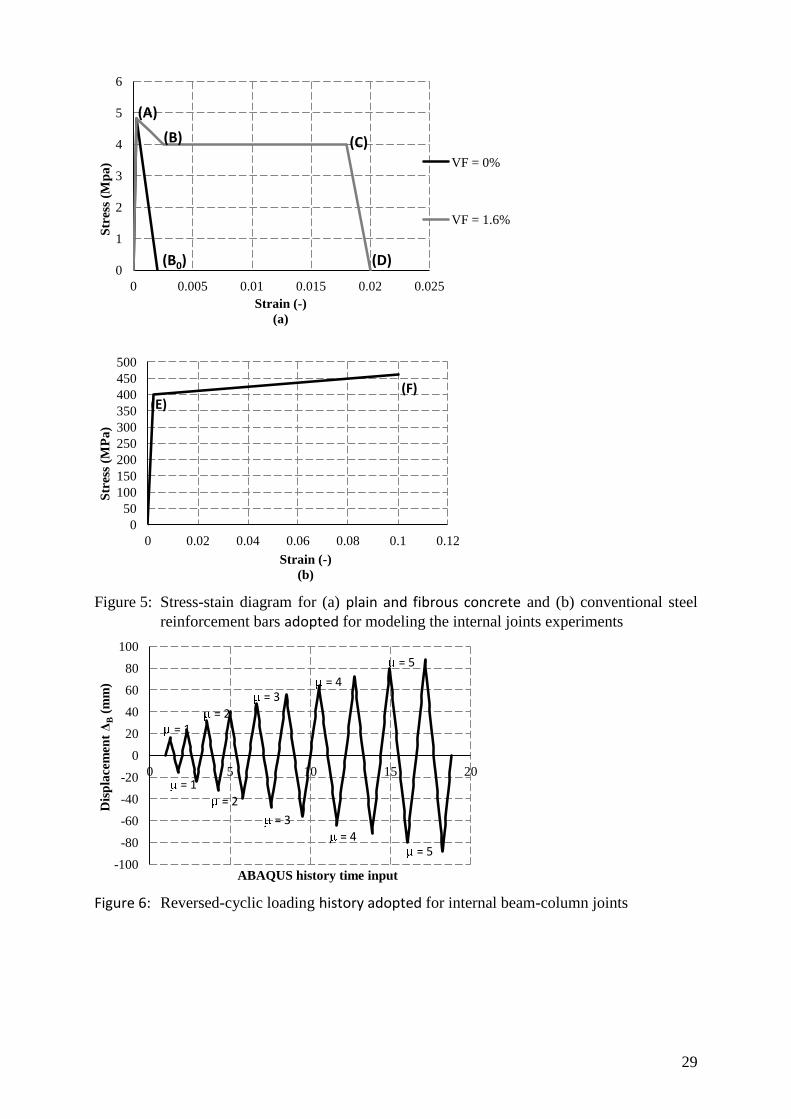
respectively. The stress-strain diagrams describing the behaviour of plain and steel fibre

reinforced concrete in tension are depicted in Fig. 5a. The stress-stain diagram describing

the behaviour of the reinforcement bars (both longitudinal and transverse) in tension and

compression is shown in Fig. 5b.

During testing both ends of the column were assumed to be simply supported in order to

simulate mid-storey inflection points (with a roller at the top to allow the application of the

axial load), while the beam has free ends. A constant axial compressive load of 670 kN was

initially imposed onto the column representing 100% gravity load of the 2nd floor of the

central column of the prototype building. Subsequently the specimen was subjected to a

reversed-cyclic loading (presented in Fig. 6) applied using a displacement-controlled

10

procedure through an arrangement of hydraulic actuators at specific locations along the

span of the beams as shown in Fig. 7. Based on Fig.7, the storey shear (Vcol) and storey drift

(Δcol) can be calculated based on the following simple expressions: Vcol=(P1l1+ P2l2)/ lcol and

Δcol=(ΔΒ1+ΔΒ2)/(l1+ l2)lcol , respectively. In the preceding equations, P1 and P2 are the

actuator forces, l1 and l2 are the distances of vertical actuators from the joint centre, ΔΒ1 and

ΔΒ2 are the vertical displacements at the loading points and lcol is the total column height

between supports (see Fig. 7).

4. FE MODELLING OF JOINT SPECIMENS

The concrete medium is modelled with a dense mesh of 8-node brick finite elements (Fig. 8).

Based on a sensitivity analysis carried out on reinforced concrete and SFRC beams [15], the

optimum dimension of the brick elements was determined to be 50 mm. The optimum mesh

size was determined based on calibration with existing experimental data (i.e. this is the

mesh which best reproduce experimental data). Reinforcement bars were modelled by 2-

noded single Gauss point truss elements and were located to match the detailing of

reinforcement used in the specimens (e.g. spacing between bars, cover distance ..etc). The

boundary conditions in the FE model of Fig. 8 also mimic the experimental ones. As

mentioned earlier, rigid elements (similar in shape and size to the steel platens used in the

experiment) were used at the supports and at the points of loading in order to better

distribute the stressed developing by the applied concentrated loads and reactions and to

avoid pre-mature localised cracking which can cause numerical instability. Furthermore, in

order to streamline the definition of the cyclic loads applied on the beams in the FE model,

the loading arrangement from the experimental work was simplified by assuming that the

distances of vertical actuators from the joint centre are equal, i.e. l1 = l2 (refer to Fig. 7).

Therefore, it can be considered that ΔΒ1 = ΔΒ2. Thus, the distance adopted in the FE analysis

was taken as the average of the two lengths considered in the experimental work. The effect

on the results is negligible as the loads are sufficiently far from the joints and surrounding

zone, which was the area of interest in terms of results.

11

5. COMPARATIVE STUDIES WITH EXPERIMENTAL DATA

5.1. Exterior beam-column joint

Fig. 9 shows the load-deflection hysteresis loops based on both the numerical predictions

and the corresponding experimental data [18] concerning the response of the external joints

depicted earlier in Fig. 1. The results describe the relationship between the reversed-cyclic

load (applied at the edge of the cantilever beam) and the vertical deflection at the same

point. The key characteristics of the curves are also summarised in a tabular from

underneath the figure. The key structural parameters summarised in the tables are the yield

load (Py) and corresponding deflection ( y), the maximum load sustained during the loading

cycles (Pmax) and corresponding deflection ( max), the load at failure (Pu) and corresponding

deflection ( u)u and the ductility ratio ( ) defined as u/ y. The comparison between the

experiment data and numerical predictions shows good agreement. However, the highest

ductility predicted by the FE analysis is about half the maximum ductility achieved in the

experiment. This is due to the difference in the number of cycles obtained (i.e. ~ 4 cycles in

the FE analysis compared to 5 in the experiment). So the ductility levels were the same for

the first 4 cycles, however the presence of the 5th cycle in the experimental data led to this

discrepancy (with the FE predictions being on the safe side). During the numerical

investigation, failure (i.e. loss of load carrying capacity) was associated with an abrupt large

increase in kinetic energy as shown in Fig. 10, indicating the presence of large/extensive

cracks within and around the joint region.

5.2. Interior beam-column joint

Figures 11 a, b and c show a comparison between the FE-based hysteresis curves –

describing the relationship between the storey shear and storey drift of the internal joints

shown in Fig. 4 – and their experimental counterparts [4] for the case of specimens S1, S2

and S3, respectively. Key values from the curves are summarised in a tabular from

underneath the figures. As in the previous case study, the comparison of the experimental

data and numerical predictions shows good agreement. Based on the results provided in

Figs 11 a to c, it is evident that the numerically predicted values of storey shear (Vy)

associated with yielding and the maximum storey shear (Vmax) associated with the ultimate

load-carrying capacity are close to their experimental counterparts with a discrepancy of less

than ~4%. Failure, however, occurs earlier during the numerical investigation, with the

beam-column joint assemblages exhibiting deformation of up to 20% lower than that

12

predicted experimentally. At this point it is important to draw a distinction between the

definitions of numerical failure and its experimental counterpart. During testing the loading

procedure ended after the specimen suffered severe destruction of concrete within and

around the joint region. On the other hand, numerical failure is considered to occur when

the structure’s stiffness matrix becomes non-positive or when an abrupt increase in kinetic

energy is observed (similar to that of Fig. 10) due to excessive cracking within and around

the joint region. During testing however, in spite the destruction of concrete, the real

structure may have still been capable of sustaining the induced excitation, by resorting

briefly to alternative resistance mechanisms, such as, for example, dowel action. This stage

of behaviour, which clearly is neither stable nor sustainable and as such of no real

significance for design purposes, is not described analytically, as the development of

alternative resistance mechanisms such as the above are not accounted for by the numerical

model. Nevertheless, the numerical model clearly serves the purpose of predicting, with

sufficient accuracy, the maximum load and displacement values attained and any differences

with their experimental counterparts are well within the accepted range of accuracy for

concrete structures, with the numerical predictions being more conservative.

Figs 12 a to c show a comparison of the experimentally established crack patterns exhibited

by specimens S1, S2 and S3 prior to failure with their numerical counterparts presented in

the form of principal strain contours. Areas of the specimens exhibiting values of principal

strain exceeding the ultimate tensile (positive) strength of SFRC of 0.02 – associated with

pull-out failure - (see point D in Fig. 5) are highlighted in grey. Areas of the specimens

exhibiting values of principal strain less than the ultimate compressive (negative) strain of

concrete (-0.0035) are highlighted in black. From Fig. 12a, specimen S1 (i.e. with Vf = 0 and

shear links that do not satisfy seismic code specifications) failed due to extensive cracking

within the joint region. Specimen S2 (i.e. with Vf = 0 and shear links that satisfy seismic code

specifications), on the other hand, failed after the formation of plastic hinges – see grey

regions in Fig. 12b – at the support of the beams of joint assemblage. This indicates that

plastic hinges develop at the roots of the beams adjoining the columns as intended in the

design. Cracking within the joint region was reduced compared to that exhibited in specimen

S1. Finally, the mode of failure of specimen S3 (i.e. the one with Vf > 0 and shear links that

do not satisfy code specifications) was similar to the mode of failure exhibited by specimen

S2 indicating that the introduction of steel fibres compensate to a large extent for the

insufficient shear links. As in the case of specimen S2, plastics hinges (see grey regions in Fig.

13

12c) form at the ends of the beams. This is a key requirement in seismic design (i.e. capacity

design concept utilising strong column–weak beam philosophy [13,28,29]. Furthermore, the

compressive strains were lower than 0.0035 suggesting that no crushing failure has

occurred.

6. PARAMETRIC STUDIES ON EXTERNAL BEAM-COLUMN JOINTS

Following the validation of the numerical predictions, parametric studies were carried out

using NLFEA to examine the potential of steel fibres to compensate for reduction in

conventional shear reinforcement. To achieve this, the spacing between shear links was

increased, whilst steel fibres were added. Therefore, the spacing between the links was

increased by SI = 0%, 50% and 100%; whilst the fibre volume fraction was increased with Vf =

0%, 1%, 1.5%, 2% and 2.5%. To account for the different fibre contents, the tensile stress-

strain diagrams for both plain and SFRC adopted are presented in Fig. 13. It is interesting to

note that strain-hardening occurs with high fibre contents such as Vf = 2.0% and 2.5%. It

must be pointed out that the fibres do not enhance the concrete cracking stress itself, but

rather the residual stress (i.e. after cracking the tensile stresses are transferred to the

fibres). Further experimental evidence for the increase in residual tensile strength can be

found elsewhere [30-32]. During the parametric investigations, the external beam-column

joint with conventional reinforcement and no fibres (i.e. Vf = 0% and SI = 0%) was selected as

the control joint specimen (CJ). The responses of all other specimen (with different fibre

content and stirrup spacing) were compared to the response of the control specimen in

order to establish the effect of the various parameters (i.e. fibre content and stirrup spacing)

on the structural response.

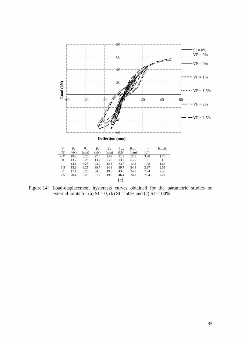
6.1. Load-deflection curves

The NLFEA-based load-deflection hysteresis curves obtained for all cases investigated are

presented in Figs 14a, b and c accompanied by the key values presented in tabular form. The

results show that the introduction of steel fibres led to an increase of load carrying capacity

and stiffness whereas the increase of the spacing of the transverse reinforcement (with SI =

50% and 100% in Figs 14b and c, respectively) resulted in a decrease of load carrying

capacity and ductility. This reduction was fully or partially recovered when introducing steel

fibres into the concrete mix. To study the hysteresis loops data further, comparisons were

made between the control joint specimen (i.e. the one with no fibres and full conventional

14

shear reinforcement) and the joints with various fibre dosages and increased stirrup spacing.

The values of the strength, ductility and energy absorption were normalised by dividing

them by the corresponding values of the control specimen. In this manner, overall

conclusions were made on the potential of fibres to compensate for reduction in

conventional transverse reinforcement. The normalised values of these key structural

performance indicators (under cyclic loading) also provide an estimate of the potential

enhancement to these parameters and the amount of fibres required to achieve them. Such

findings are useful for loading types which are characterised by their cyclic nature, such as

seismic loads.

6.2. Strength

Fig. 15a shows the variation of the ratio between the load carrying capacity Pmax of each joint

considered during the parametric studies and that of the control joint specimen (Pmax,0)

plotted against the fibre content Vf for different spacing increases. Similarly, Fig. 15b shows

the variation of the ratio between the load at yield Py of each specimen and that of the

control joint (Py,0) plotted against Vf and SI. The graph shows that the strength consistently

increases as e more fibres are added. The predictions presented in Figs 15 a, b show that

increasing the stirrups spacing reduced the capacity of the conventionally-reinforced

concrete joint (Vf = 0%) to sustain further loading, e.g. for joints with SI = 50%, a reduction of

18% in Py and 11% in Pmax compared to the control joint is observed. Similarly, for joints with

SI = 100% and no fibres the decrease in Py and Pmax is about 28% and 59%, respectively, of

their control specimen counterparts. On the other hand, adding fibres resulted in elevated

values of Py and Pmax (e.g. increasing the fibre content for joints with SI = 0% resulted in an

increase of Py and Pmax by up to 47% and 41% of Py,0 and Pmax,0 respectively. Similarly, for

joints with SI = 50% and 100% increasing Vf resulted in elevated values of Py (by up to 52%

and 55% for joints with SI = 50% and 100%, respectively) and Pmax (by up to 76% and 33% for

joints with SI = 50% and 100%, respectively). The strength level of the control specimen was

restored with fibre contents of Vf = 0.5% and 1.3% for joints with and 100%,

respectively. Higher fibre amounts led to the strength level of the control specimen been

exceeded by up to 40~60%. Similarly, the yield load of joints with SI = 50% and 100% reached

that of the control specimen Py,0 when fibres were added at Vf = 1.7% and 2.2%, respectively.

6.3. Ductility

The variation of the ductility of each joint µ normalised to that of the control joint (µ,o) for

15

different values of Vf and SI is presented in Fig. 16a. The results demonstrate that that the

ductility performance of the joints with increased stirrups spacing (but without fibres added

to compensate) deteriorated considerably. The results also show that ductility increases as

the amount of fibres is increased. The trend, however, is true up to a critical value (or limit)

of fibre volume fraction beyond which the ductility begins to reduce. It is also interesting to

note that the higher the spacing between the stirrups, the higher the critical fibre volume

ratio. This suggests that the addition of fibres within an optimum range enhances ductility.

However, fibres should not be provided in excessive quantities as this will lead to a stiffer

response with the joint deflecting less (this is largely due to the fibres role in bridging across

cracks and limiting their opening). This crack control and confinement effect is most

pronounced in when fibres are provided in addition to full conventional shear reinforcement

(i.e. SI = 0%). The optimum amounts of fibres were found to be approximately Vf = 1% for

SFRC joints with SI = 0%, Vf = 2% for joints with SI = 50% and 100% (with being twice that of

the control specimen). For SFRC joints with SI = 50% and 10%, the ductility level of the

control specimen was attained with fibres provided at Vf = 1.5%.

Therefore, it can be concluded that the addition of fibres in optimum amounts will lead to

significant enhancement to ductility. This is of particular relevance to seismic design as

ductility is one of the main considerations to ensure sufficient energy dissipation (energy

absorption was also studied and the results are presented subsequently). Nevertheless,

fibres should not be provided in excess of the optimum amounts as this will lead to a less-

ductile response as mentioned earlier (the response could potentially be improved by

adjusting the mix design, however this is beyond the scope of the present paper). Therefore,

fibres could be provided to replace some of the conventional shear reinforcement (and thus

lessen the congestion of shear links in critical regions), but should not be provided in

addition to full conventional reinforcement.

6.4. Energy absorption ratio

Fig. 16b shows the variation of the energy absorbed by each joint (Ea) until failure due to

nonlinear behaviour (owing to cracking of concrete and yielding of the steel bars) normalised

by the energy absorption of the control joint (Ea,0 ) for different values of Vf and SI. The trend

is similar to the one observed earlier for ductility with energy absorption increasing up to a

certain peak and then dropping if excessive amounts are provided. The optimum fibre

content associated with the highest levels of energy absorption were Vf = 1% for joints with

16

SI = 0% and Vf = 2% for joints with SI = 50% and 100%. It should be noted that the

enhancement in energy absorption due to fibres is significant (with absorption levels 4~10

times higher than those associated with the control specimen).

6.5. Principal strain contours and cracking patterns

In order to gain better insight into how steel fibres affect the responses of the joints,

attention was focussed on the distribution of principal strains which is presented in the form

of contours and vectors in Figs 17 to 20 for different levels of loading. The graphs were

developed to study the control joint specimen with SI = 0% at three levels of fibre content

(i.e. Vf = 0%, 1% and 2%) and at different deflection points from yield to failure. The strain

vectors are useful in indicating the pattern of crack formation. For presentation purposes,

the upper limit value of tensile (positive) strain is set equal to 0.000239 which is associated

with crack formation (i.e. Point A in Fig. 13), whereas the lower limit for compressive

(negative) strain is set at -0.0035 representing the ultimate compressive strain for plain

concrete. Thus the regions of the joint assemblage exhibiting tensile strains equal or larger

than the above upper limit were highlighted in grey to indicate cracking zones.

The distribution of principal strains at yield (i.e. δy = 6.25 mm), taken at the end of the first

cycle, are illustrated in Fig. 17. The contours indicate that cracking has been reduced as fibre

amount provided increases. This is supported by the graphs of principal strain vectors which

also show that the crack formation is less in joints with higher fibre amounts. This confirms

the role of fibres in controlling crack opening. Similar conclusions are drown from Fig. 18

showing the distribution of the principal strains contours and vectors at the end of the

second load cycle (δ2 = 12.5 mm). It should be noted that in latter figures the grey area are

associated with tensile strains higher than 0.001, which is the ultimate tensile strain for plain

concrete (see point B0 in Fig. 13). It can be seen that the crack formation is limited with Vf =

2% as compared to the results of specimens with less amounts of fibre.

Figure 19 shows the distribution of the principal strain contours and vectors at the end of

the third cycle with a deflection δ3 = 24.9 mm. At this level of loading (deformation) the

numerical analysis predicted that the joint with fibre contents Vf = 0% and 2% suffered loss

of load carrying capacity. The joint with Vf = 1% (optimum amount of fibres) was able to

undertake additional loading and failed later in the loading process at the end of the forth

cycle (at δ4 = 49.9mm) and the corresponding contours and vectors are depicted in Fig. 20. It

should be noted, that the regions highlighted in grey in Figs 19 and 20 are associated with

17

tensile strains higher than the ultimate tensile strain for SFRC of 0.02 (i.e. point D in Fig. 13)

indicating pull-out failure of the fibres. The results show that increasing the values of Vf led

to limited zones of pull-out failure. A similar trend of structural response to those described

above is also observed for the joints with SI = 50% and 100%.

6.6. Mode of failure

The mode of failure of all joint assemblages considered in the present parametric studies can

be observed using the principal strain contours at failure shown in Figs 21 to 23. In these

graphs, the regions of the specimen highlighted in grey denote areas where the ultimate

tensile strain associated with pull-out failure of 0.02 has been exceeded (i.e. point D in Fig.

13). The only exception is the joints without fibres (i.e. Vf = 0%), where the tensile strain

associated with cracking of 0.001 for plain concrete is used to define the grey zone. The

ultimate compressive strain of -0.0035 is adopted to indicate crushing failure and the

corresponding intervals are highlighted in black. Figs 21 to 23 show that all joints with no

fibres suffered extensive cracking even within the joint region prior to failure. The

introduction of fibres resulted in a reduction of cracking within and around the joint region.

As the fibre content was increased, the regions of the joint assemblage exhibiting pull-out

failure reduced and for the majority of cases investigated the failures were limited to the

beam ends, but did not extend into the column or joint region. This indicates that in SFRC

joints, plastic hinges will form at the end of the beam – and not on the column – which is of

particular relevance to seismic design (i.e. capacity design based on strong column-weak

beam philosophy). Additionally, it was found that the extent of cracking suffered in the joint

region was significantly reduced as fibres were added.

7. PARAMETRIC STUDIES ON INTERNAL BEAM-COLUMN JOINTS

Parametric investigations, similar to those carried out for external joints, were carried out

for the case of the internal joints. The internal joint specimen S2, designed in accordance to

seismic code specifications with a dense arrangement of double stirrups and no fibres (i.e. Vf

= 0% and SI = 0%), was selected as the control joint specimen. Comparing the structural

response of the control joint with that of the SFRC joints with reduced conventional

transverse reinforcement provided an insight into the potential for steel fibres to help lessen

the congestion of stirrups. From Figs 4c,d it can be seen that both the column and beam

cross-sections of the control specimen have a dense arrangement of double stirrups in order

18

to safeguard against shear failure and ensure an acceptable level of ductility (due to

confinement). In the present study, the amount of conventional transverse reinforcement

was reduced in three ways as follows:

(i) increase in the stirrups spacing (i.e SI = 50%)

(ii) increase in the stirrups spacing (i.e. SI = 100%)

(iii) decrease in the hoops area from double stirrups to single stirrups in the columns

(so the stirrups provided at 45o to the column sides, see Fig. 4c, were removed)

but no increase in spacing

The scenarios in (ii) and (iii) above lead to the same level of reduction in transverse

reinforcement, i.e. amount halved. However, the removal of the inner stirrups provided

insight into the potential of fibres to compensate for the loss of confinement provided by

the double-stirrup arrangement, which is an important consideration in seismic design

detailing. The latter also requires the spacing between stirrups to be within certain limits to

ascertain adequate confinement. Fibres provide enhancement to confinement by controlling

crack opening as they bridge the cracks. The current investigation examined whether or not

this confinement is sufficient to compensate for the reduced conventional hoops (either by

relaxing spacing or using single stirrups). During the present parametric investigations, as the

conventional transverse reinforcement was reduced, steel fibres were added to compensate

with Vf = 0%, 1%, 1.5%, 2% and 2.5%. The tensile stress-strain diagrams adopted for both

plain and fibrous concrete adopted are presented in Fig. 24.

7.1. Storey shear-drift curves

The storey-shear versus storey-drift hysteresis curves obtained for all cases investigated are

presented in Figs 25 to 27 accompanied by a summary of the key values in tabular form. Vy

and Δy are the storey shear and storey drift at yield, Vmax and Δmax are the maximum storey

shear sustained during the loading cycles and its corresponding storey drift, Vu and Δu are

the ultimate storey drift at failure and corresponding storey shear, is the ductility ratio

defined as = Δu/Δy. The figures show that the introduction of steel fibres generally results

in an increase in ultimate load carrying capacity and stiffness. On the other hand, the

reduction of the stirrups resulted in a decrease of load carrying capacity and ductility. This

reduction, as discussed in detail in the following sections, is fully or partially recovered when

introducing steel fibres into the concrete mix.

19

7.2. Strength

The curve presented in Fig. 28a shows the variation of the maximum storey shear of internal

joints Vmax normalised to that of the control joint specimen (Vmax,0) for different values of

fibre content and the spacing of stirrups. The predictions presented in Fig. 28a confirm the

potential of fibres to safeguard and to enhance the strength of internal joints. In comparison

to the strength of the control joint, Vmax increased by up to 53% for joints with single

stirrups, 43% and 58% for joints with SI = 50% and 100%, respectively. The strength level of

the control specimen was restored when fibres were added at Vf = 0.5% for joints with single

stirrups or with SI = 50% and at Vf = 1% for joints with SI = 100%. Further, increase of load-

carrying capacity was achieved (exceeding that of the control specimen level by ~50%) with

higher fibre dosages. Similarly to Fig. 28a, the curves shown in Fig. 28b present the variation

of the storey shear associated with the load at yield Vy normalised to that the corresponding

values for the control specimen for different values of Vf and SI. Again it is clear that fibres

enhance the load at yield, with the increase in Vy being up to 10% on average.

7.3. Ductility and stiffness

Figure 29a presents the variation in ductility of the structural configurations studied in the

present parametric investigations normalised by the ductility of the control specimen for

different values of Vf and SI. The results show that the addition of steel fibres improves

ductility up to a certain level of fibre content. Beyond this level, a further increase of the

fibre content leads to a reduction of ductility. This is a finding that has been realised earlier

when examining the exterior joint. For instance in the joints with single stirrups, the highest

ductility increase was observed when fibres were added at Vf = 1% ~ 1.5%. Similarly, the

optimum fibre contents were found to be at Vf = 1% for both joints with SI = 50% and 100%.

The ductility level of the control specimen (i.e. the one with full conventional transverse

reinforcement and no fibres) was restored for both joints with SI = 50% and those with single

stirrups when fibres were added with Vf = 0.5% and 0.75%, respectively. However, the

ductility level of the control specimen could not be restored for joints with SI = 100% even

for a high value of fibre content with Vf = 2.5%. In the latter case only about 80% of the

control specimen ductility level was restored. This indicates the severity of conventional

steel reduction in this case where the spacing between the stirrups has been doubled. This

also shows that, from a ductility viewpoint this case is worse than using single stirrups

instead of double ones, as a way of reducing transverse reinforcement congestion. The

double-stirrups arrangement is usually provided to enhance confinement. This demonstrates

20

that fibres can provide sufficient confinement to allow the use of single stirrups. On the

other hand, the loss in confinement due to doubling the spacing of stirrups is too severe to

be restored using fibres in the case studied.

7.4. Energy absorption ratio

The energy absorption capacity calculated for the interior joints Ea was normalised to the

energy absorption of the control specimen (Ea,0) as presented in Fig. 29b. The optimum fibre

contents coinciding with highest energy absorption levels were found to be Vf = 1.5%. for

specimens with single stirrups and Vf = 1.0% for SI = 50% and 100% The energy absorption

level of the control specimen was restored for all joints except those with SI = 100% This

suggests that the high increase in stirrup spacing by 100% could not be fully compensated

through the use of steel fibres in the present case considered.

7.5. Principal strain contours and cracking patterns

In order to study the structural responses further, the FE-based principal strain contours and

vectors were established at deflection levels of: (i) Δy (associated with yielding), (ii) Δmax

(associated with maximum load carrying capacity) and (iii) Δu (maximum deformation

exhibited prior to failure) as presented in Figures 30, 31 and 32, respectively. The samples

were taken for the joints with SI = 50% at varying fibre content levels, i.e. Vf = 0%, 1% and

2%. Strain vectors are also presented in the figures and they are also useful in indicating the

pattern of crack formation.

The distribution of the principal strains and vectors depicted in Fig. 30 is taken at the end of

the first cycle, at which point yielding occurs (i.e. Δy = 28.6mm). In these figures the upper

limit of the strains was selected to coincide with the tensile – positive – strain associated

with the onset of cracking (i.e. 0.00024, see point A in Fig. 24) and the ultimate compressive

– negative – strain (i.e. -0.0035). Thus, the areas highlighted in grey indicate crack initiation.

It can be seen that the principal strain for the joint with no fibres was the highest amongst

all, while the strain has reduced as fibre amounts were increased indicating that crack

control has been provided.

Figure 31 shows the distribution of the principal strains and vectors when the specimen

attain their maximum load carrying capacity (i.e. Δmax= 69.4mm). It should be noted that the

regions of the joint with Vf = 0% highlighted in grey are associated with tensile strains higher

than 0.002 (ultimate tensile strain for plain concrete, see point B0 in Fig. 24), while for SFRC

21

joints with Vf = 1% and 2% the grey regions indicate strain values exceeding 0.01

(approximately half the ultimate strain of SFRC). Again, it can be seen strains as well as

cracking reduce with increasing values of fibre content.

The principal strain distribution at the point of failure (i.e. Δu = 100.2mm) is presented in

Figure 32. In this case the grey region now indicates tensile strains higher than 0.02, which is

the ultimate tensile strain exhibited SFRC and is associated with pull-out failure of the fibres

(point D, in Figure 24). The principal strain contours and vectors indicate that the crack

opening is better controlled as the fibre content is increased and that pull-out failure occurs

in increasingly limited regions of the SFRC joints (compared to an extensive grey area on the

joint without fibres showing that the latter experienced wider crack opening). Finally it is

interesting to see that for SFRC, pull-out failure occurred in limited zones at the ends of the

beams, and not on the column or joint itself, which is desirable in seismic design.

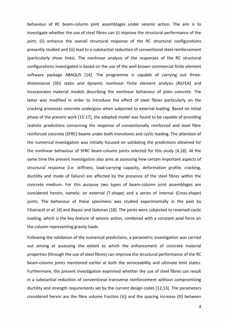
7.6. Mode of failure

The numerically predicted values of principal strain prior to failure presented in the form of

contours for all internal joints considered in this parametric investigation are presented in

Figs 33 to 35. The contours intervals were selected so that the strains exceeding the ultimate

tensile strength of SFRC of 0.02 were highlighted in grey, indicating pull-out failure. Similarly,

strains higher than the ultimate compressive strain of -0.0035 were highlighted in black. The

contours show that pull-out failure in SFRC joints occurred in limited regions compared to

the extensive grey zones on the specimens without fibres (see Figs 33a, 34a and 35a). This

comparison reveals that the latter the specimens exhibited wider cracks over more extended

areas. It is interesting to see that pull-out failure occurred at the ends of the beams and not

within the column or joint itself. This indicates that plastic hinges formed at the ends of the

beams thus satisfying the strong-column weak-beam philosophy adopted by Eurocode 8 [13]

for the seismic design of RC frames.

8. DESIGN CONSIDERATIONS

An attempt was made to quantify the fibre dosage needed to replace a given amount of

stirrups, yet retaining a certain level of strength and ductility (i.e. the most critical

parameters for seismic design). To demonstrate the basic idea, the results of the forgoing

parametric studies on external joints were reproduced in the form of contour diagrams as

shown in Fig. 36. The contours depict the effect of reducing the stirrups amount (rsw) whilst

22

increasing the fibre content Vf on the ductility ratio and the load-carrying capacity Pmax for

the case of external joint. Similarly to current codes of practice [12,13], the stirrup content is

expressed as a ratio between the stirrups area and their spacing, i.e. Asw/S. Subsequently,

the reduction in conventional shear reinforcement was defined as the ratio of the stirrup

area and spacing normalised by the corresponding ratio of the control specimen (the latter

denoted by a zero subscript), i.e. rsw = (Asw/S)/(Asw,0/Srw,0). On the contour plots, the control

specimen results are those associated with full conventional reinforcement and no fibres, i.e.

rsw = 1 and Vf = 0%.

Fig. 36a indicates that μ decreases when Vf > 2%, as mentioned earlier (see Fig. 16). From the

contour plots, it can also be seen that the ductility ratio associated with the control joint

specimen of (i.e. = 4) can be maintained along a line linking points rsw = 1 and Vf = 0% at

one end and rsw = 0.5 and Vf = 2% at the other. For clarity, this is shown as a dotted line on

Fig. 36a. Similarly, the Pmax value associated with the control specimen can be maintained

along a line linking points rsw = 1 and Vf = 0% and rsw = 0.5 and Vf = 1.3%. However, for design

purposes the more stringent line determined for ductility must be adopted to ensure both

strength and ductility levels of the control specimen are maintained (both lines are plotted

on Fig. 36b). Subsequently, a simplified design criterion was proposed and was defined by

the straight line linking points rsw = 1 and Vf = 0% and rsw = 0.5 and Vf = 2%. Thus, the

proposed line can be expressed as: Vf(%) = 4(1 – rsw) where Vf is the volume fraction of fibres

required to replace a given reduction in conventional transverse reinforcement expressed in

terms of the ratio of the stirrups content rsw. As stated earlier, this attempt was made mainly

to demonstrate the basic principle behind the proposed design concept, nevertheless

further studies on different joint types along with field calibrations are needed before any

design equations can be recommended for the use of practicing engineers.

9. CONCLUSIONS

In spite of its simplicity, the proposed NLFEA model presently employed was capable of

yielding realistic predictions of the response of a number of internal and external beam

column joints under reversed-cyclic loading (which is the key feature of seismic action).

Initially, the numerical predictions were calibrated using existing experimental data to

ascertain the accuracy of the numerical results and subsequently full parametric studies

were carried out to examine the potential for steel fibres to compensate for a reduction in

23

conventional transverse reinforcement (suggested to lessen congestion of such

reinforcement, especially in seismic design). Key structural response indicators such as

strength, cracking, ductility and energy absorption were studied. The results of each SFRC

joint were normalised by dividing them by the corresponding values associated with the

control joint specimen (i.e. the one with full conventional transverse reinforcement and no

fibres). This helped formulate the following conclusions and recommendation:

Addition of steel fibres improved the strength consistently as the amount of fibres

was increased. Fibres were also effective in controlling crack propagation. Pull-out

failure was found to be at the ends of the beams (and not within the columns or joint

itself), which indicates that plastic hinges formed at these locations. This is desirable

in earthquake-resistant design.

The addition of fibres in optimum amounts led to significant enhancement to

ductility. This is of particular relevance to seismic design as ductility is one of the

main considerations to ensure sufficient energy dissipation (energy absorption was

also studied and the results were consistent with ductility findings). Nevertheless,

fibres should not be provided in excessive amounts as this will lead to a less-ductile

response.

For exterior joints, the ductility level of the control specimen was restored with fibres

added at Vf = 1.5%. For interior joints, the ductility level of the control specimen was

restored for both joints with single stirrups and those with SI = 50% when fibres were

added with Vf = 1%. However, the ductility level of the control specimen could not

restored for the joint with SI = 100%, even when fibres were provided at dosages as

high as Vf = 2.5%. This indicates the severity of conventional steel reduction in this

case where the spacing between the stirrups has been doubled. The double

arrangement is usually used to ensure sufficient confinement is provided. Thus the

results show that fibres can provide sufficient confinement to allow the use of single

stirrups. However the loss in confinement due to doubling the spacing of stirrups is

too severe to be restored using fibres in the case studied.

In summary, it can be concluded that steel fibres provided in optimum amounts can

substitute for conventional transverse reinforcement and thus allow for a relaxation in

stirrups congestion often experienced in seismic detailing of beam-column joints. A

simplified design equation was also developed to determine the fibre content needed to

replace a given amount of stirrups whilst retaining the same level of strength and ductility.

24

REFERENCES

1. Ehsani MR, Wight JK. Effect of transverse beams and slab on behaviour of reinforced

concrete beam to-column connections. ACI Jnl 1985;82:188–195

2. Ehsani MR, Wight JK. Exterior reinforced concrete beam-to-column connections

subjected to earthquake-type loading. ACI Jnl 1985;82:492–499

3. Tsonos AG, Tegos IA, Penelis GGR. Seismic resistance of type 2 exterior beam-column

joints with inclined bars. ACI Struct Jnl 1992;89(1):3–12

4. Filiatrault A, Pineau S, Houde J. Seismic Behaviour of Steel Fiber-Reinforced Concrete

Interior Beam-Column Joints. ACI Struct Jnl 1995;92(5):543–552.

5. Tsonos AG. Cyclic load behaviour of reinforced concrete beam–column subassemblages

designed according to modern codes. Eur Earthq Eng 2006;3:3–21

6. Tsonos AG. Cyclic load behavior of reinforced concrete beam–column subassemblages

of modern structures. ACI Struct Jnl 2007;104:468–478

7. Kotsovou G, Mouzakis H. Seismic behaviour of RC external joints, Mag Concr Res

2011;63(4):247–264.

8. Kotsovou G, Mouzakis H. Seismic design of RC external beam-column joints. Bull Earthq

Eng 2012;10(2):645–677.

9. Cotsovos DM and Kotsovos MD. Cracking of rc beam / column joints: Implications for

practical structural analysis and design. The Struct Eng 2008;86(12):33–39.

10. Fleury F, Reynouard JM and Merabet O. Finite element implementation of a steel-

concrete bond law for nonlinear analysis of beam-column joints subjected to

earthquake type loading. Struct Eng & Mech 1999;7(1):35–52.

11. Lykidis GCh and Spiliopoulos KV. 3D Solid Finite Element Analysis of Cyclically Loaded RC

Structures Allowing Embedded Reinforcement Slippage. Jnl Struct Eng ASCE

2008;134:629–638.

12. EN1992-1 Eurocode 2. Design of Concrete Structures—Part 1-1. General Rules and Rules

for Buildings. Brussels: European Committee for Standardization; 2004.

25

13. EN 1998-1 Eurocode 8. Design of Structures for Earthquake Resistance—Part 1. General

Rules, Seismic Actions and Rules for Buildings. Brussels: European Committee for

Standardization; 2004.

14. ABAQUS Version 6.7 Documentation; 2007. Accessed online at

http://www.engine.brown.edu:2080/v6.7/index.html

15. Syed Mohsin SM. Behaviour of fibre-reinforced concrete structures under seismic

loading. PhD thesis. Imperial College London; 2012.

16. Abbas AA, Syed Mohsin SM, Cotsovos DM. Numerical modelling of fibre reinforced

concrete. Proceedings of the International Conference on Computing in Civil and

Building Engineering icccbe 2010, Nottingham, UK (Tizani W. (ed)). University of

Nottingham Press; 2010, Paper 237, p. 473, ISBN 978-1-907284-60-1.

17. Abbas AA, Syed Mohsin SM, Cotsovos DM. A comparative study on modelling

approaches for fibre-reinforced concrete. Proceedings of the 9th HSTAM International

Congress on Mechanics. Limassol, Cyprus, 12-14 July; 2010.

18. Bayasi Z, Gebman M. Reduction of Lateral Reinforcement in Seismic Beam-Column

Connection via Application of Steel Fibres. ACI Struct Jnl 2002;99(6):772–780.

19. Kotsovos MD, Pavlovic MN. Structural concrete: Finite-element analysis for limit-state

design. London: Thomas Telford; 1995.

20. RILEM Technical Committees. RILEM TC 162-TDF: Test and Design Methods for Steel

Fibre-Reinforced Concrete, Recommendation: Design Method. RILEM Mater and

Struct 2000;33:75–81.

21. RILEM Technical Committees. RILEM TC 162-TDF: Test and Design Methods for Steel

Fibre-Reinforced Concrete, Final Recommendation: Design Method. RILEM Mater

and Struct 2003;36:560–567.

22. Barros JAO, Figueiras JA. Flexural behavior of SFRC: Testing and modelling. Jnl Mater in

Civ Eng ASCE 1999;11(4):331–339.

23. Barros, JAO, Figueiras JA. Model for the Analysis of Steel Fibre Reinforced Concrete

Slabs on Grade. Comput and Struct 2001;79(1):97–106.

24. Tlemat H, Pilakoutas K, Neocleous K. Modelling of SFRC using Inverse Finite Element

Analysis. RILEM Mater and Struct 2006;39:221–233.

26

25. Lok TS, Pei JS. Flexural Behavior of Steel Fiber-Reinforced Concrete. Jnl Mater in Civ Eng

ASCE 1998;10(2):86–97.

26. Lok TS, Xiao JR. Flexural Strength Assessment of Steel Fiber-Reinforced Concrete. Jnl

Mater in Civ Eng ASCE 1999;11(3):188–196.

27. NRCC. National Building Code of Canada, Associate Committee on the National Building

Code, National Research Council of Canada, Ottawa, ON; 1990.

28. Booth E, Key D. Earthquake Design Practice for Buildings. 2nd ed. London: Thomas

Telford; 2006.

29. Elghazouli AY. Seismic Design of Buildings to Eurocode 8. Oxon: Spon Press; 2009.

30. Lim DH and Oh BH. Experimental and theoretical investigation on the shear of steel fibre

reinforced concrete beams. Eng Struct 1999;21(10):937–944.

31. Yazici S, Inan G and Tabak V. Effect of aspect ratio and volume fraction of steel fiber on

the mechanical properties of SFRC. Construct and Build Mater2007;21(6):1250–1253.

32. Chalioris CE and Karayannis CG. Effectiveness of the use of steel fibres on the torsional

behaviour of flanged concrete beams. Cement and Conc Compos2009;31(5):331–341.

27

Figure 1: Geometry and reinforcement details for the external (T-shape) beam-column joint

tested by Bayasi and Gebman [18] – all dimensions are in mm

Figure 2: Stress-stain diagram for (a) SFRC and (b) conventional steel reinforcement bars

adopted for the numerical modeling of the external joint experiments

0

0.5

1

1.5

2

2.5

3

3.5

0 0.005 0.01 0.015 0.02 0.025

Str

ess

(MP

a)

Strain (-)

(a)

VF = 2%

(A)

(B) (C)

(D)

0

50

100

150

200

250

300

350

400

450

500

0 0.02 0.04 0.06 0.08 0.1 0.12

Str

ess

(MP

a)

Strain (-)

(b)

(E) (F)

(b) (a)

610

305

254 (2) 15.9 mm & (1) 12.7

mm

(3) 12.7 mm

9.5 mm @ 152 mm c/c

483

(4) 15.9 mm

9.5 mm @ 152 mm c/c 254

254

28

Figure 3: Reversed-cyclic loading history applied to external beam-column joints

Figure 4: Details of (a) specimens S1 and S3, (b) specimen S2, (c) column cross-section and

d) beam cross-section tested by Filiatrault et al. [4] – all dimensions are in mm

-150

-100

-50

0

50

100

150

0 2 4 6 8 10 12

Def

lect

ion

(m

m)

ABAQUS input time

(c)

COLUMN 400*400 mm

CONFINED REGION

70

60

70

70

70

60

COLUMN 400*400 mm

UNCONFINED

REGION

70

70

70

60

70

60

15M

(d)

80 70 70

60

335

45

60

80 100

BEAM 500*400

mm

10M

130

(a)

400 1950

SPECIMEN S1,

S3

1950

9 t

ies

@

150

c/c

1370

500

1365

135

9 t

ies

@

150

c/c

2 single ties in the joint

4-15M 4-15M

4-15M

16-20M

FRC in this Region

(S3 only)

9 double ties

@ 200 c/c

(b)

400

130

1950

SPECIMEN S2

1950

7 d

oub

le

ties

@

85 c

/c

1370

500

1365

135

16 d

ou

ble

tie

s

@ 8

5 c

/c

5 double ties in the

joint 4-15M 4-15M

4-15M

16-20M

double ties

@ 200 c/c

Sin

gle

ties

@

150

c/c

9 double ties

@ 100 c/c

29

Figure 5: Stress-stain diagram for (a) plain and fibrous concrete and (b) conventional steel

reinforcement bars adopted for modeling the internal joints experiments

Figure 6: Reversed-cyclic loading history adopted for internal beam-column joints

0

1

2

3

4

5

6

0 0.005 0.01 0.015 0.02 0.025

Str

ess

(Mp

a)

Strain (-)

(a)

VF = 0%

VF = 1.6%

(A)

(B0) (D)

(B) (C)

0

50

100

150

200

250

300

350

400

450

500

0 0.02 0.04 0.06 0.08 0.1 0.12

Str

ess

(MP

a)

Strain (-)

(b)

(E) (F)

-100

-80

-60

-40

-20

0

20

40

60

80

100

0 5 10 15 20

Dis

pla

cem

ent Δ

B (

mm

)

ABAQUS history time input

= 1

= 1

= 2

= 2

= 3

= 3

= 4

= 4

= 5

= 5

30

Figure 7: Loading arrangement of cyclic (left) and reversed-cyclic (right) loading used for the

internal beam-column joint

Figure 8: FE mesh adopted for modeling internal beam-column joints

Beam-column

joint

Py

(kN) y

(mm)

Pu

(kN) u

(mm)

Pmax

(kN) Pmax

(mm) u/ y Pmax/Py

Experimental

18.5 6.25 23.3 100 50.9 50 16.0 2.75

FE model

19.3 6.25 50.0 49.6 50.0 49.6 7.94 2.59

Figure 9: Load-deflection hysteresis curves for external joints showing both numerical

and experimental results

-60

-40

-20

0

20

40

60

-150 -100 -50 0 50 100 150

Lo

ad

(k

N)

Deflection (mm)

Experimental

FE model

P2

P1

Axial force

l 1

l 2

ΔΒ

1

ΔΒ

2

lcol

ΔΒ

2 ΔΒ

1 P2

P1

Axial force

l 1

l 2 lcol

31

Figure 10: Kinetic energy variation during loading of the external joint

Vf

(%) Vy

(kN)

Δy

(mm) Vmax (kN)

ΔVmax

(mm) Vu

(kN)

Δu

(mm) = Δu/Δy Vmax/ Vy

Experiment 109.4 28.2 149.8 72.9 127.9 137.6 4.88 1.37

FE model 109.3 28.6 154.9 73.0 132.1 116.8 4.08 1.42

(a)

0

5000

10000

15000

20000

25000

30000

35000

0 1 2 3 4 5

Kin

etic

en

erg

y

Number of cycles

-200

-150

-100

-50

0

50

100

150

200

-200 -150 -100 -50 0 50 100 150 200

Sto

rey

sh

ear,

Vco

l (

kN

)

Storey drift , Δcol(mm)

Experimental

FE model

μ=1

μ=3 μ=2

μ=1

μ=4 μ=3 μ=2

μ=5

μ=5 μ=4

32

Vf

(%)

Vy

(kN)

Δy

(mm) Vmax

(kN)

ΔVmax

(mm) Vu

(kN)

Δu

(mm) =

Δu/Δy Vmax/

Vy

Experiment 109.4 27.6 148 73.8 144.3 123.8 4.49 1.35 FE model 92.4 28.8 143.1 84.3 124.2 140.8 4.9 1.55

(b)

Vf

(%)

Vy

(kN)

Δy

(mm) Vmax

(kN)

ΔVmax

(mm) Vu

(kN)

Δu

(mm) =

Δu/Δy Vmax/

Vy

Experiment 123.9 28.7 170.1 73.6 140.0 147.9 5.15 1.37

FE model 122.4 28.6 168.0 102.2 162.7 116.8 4.08 1.37

(c)

Figure 11: Numerical and experimental results of storey shear-storey drift curves for

internal joints (a) S1, (b) S2 and (c) S3

-200

-150

-100

-50

0

50

100

150

200

-200 -150 -100 -50 0 50 100 150 200

Sto

rey

sh

ear,

Vco

l (k

N)

Storey drift, Δcol (mm)

Experimental

FE model

μ=4 μ=3 μ=2

μ=1

μ=5

μ=4 μ=3 μ=2

μ=1

μ=5.4

-200

-150

-100

-50

0

50

100

150

200

-200 -150 -100 -50 0 50 100 150 200

Sto

rey

sh

ear,

Vco

l (k

N)

Storey drift, Δcol (mm)

Experimental

FE model

μ=4 μ=3 μ=2

μ=1

μ=3 μ=2

μ=1

μ=4 μ=5

μ=5

33

(a)

(b)

(c)

Figure 12: Comparison of experimentally established and numerically predicted crack

patterns exhibited prior to failure for internal joints (a) S1, (b) S2 and (c) S3

Figure 13: SFRC tensile stress-strain diagrams adopted for the parametric studies on external

(T-shape) beam-column joints

0

0.5

1

1.5

2

2.5

3

3.5

4

0 0.005 0.01 0.015 0.02 0.025

Str

ess

(MP

a)

Strain (-)

VF = 0%

VF = 1%

VF = 1.5%

VF = 2%

VF = 2.5%

(A)

(B0)

(B)

(D)

(C)

34

Vf (%)

Py (kN)

y

(mm) Pu

(kN) u

(mm) Pmax (kN)

Pmax

(mm)

u/ y Pmax/Py

0 18.2 6.25 27 24.9 31.9 12.5 3.98 1.75

1 20.4 6.25 40.6 49.9 40.6 49.9 7.98 1.99

1.5 22.0 6.25 44.1 49.8 44.1 49.8 7.97 2.01

2 24.1 6.25 42.6 24.9 45.8 12.4 3.98 1.90

2.5 26.7 6.25 44.9 24.9 50.3 12.4 3.98 1.88

(a)

Vf

(%)

Py

(kN) y

(mm)

Pu

(kN) u

(mm)

Pmax

(kN) Pmax

(mm) u/ y Pmax/Py

CJ* 18.2 6.25 27 24.9 31.9 12.5 3.98 1.75

0 15.0 6.25 28.4 12.4 28.4 12.4 1.98 1.89

1 15.8 6.25 35.5 24.8 35.5 24.8 3.97 2.25 1.5 17.6 6.25 37.1 24.8 42.7 27.6 3.97 2.62

2 19.3 6.25 50.0 49.6 45.21 24.8 7.94 2.34 2.5 22.8 6.25 47.6 24.8 47.6 24.8 3.97 2.09

(b)

-60

-40

-20

0

20

40

60

-60 -40 -20 0 20 40 60

Lo

ad

(k

N)

Deflection (mm)

VF = 0%

VF = 1%

VF = 1.5%

VF = 2%

VF = 2.5%

-80

-60

-40

-20

0

20

40

60

-60 -40 -20 0 20 40 60 Lo

ad

(k

N)

Deflection (mm)

SI = 0%,

VF = 0%

VF = 0%

VF = 1%

VF = 1.5%

VF = 2%

VF = 2.5%

35

Vf

(%)

Py

(kN) y

(mm)

Pu

(kN) u

(mm)

Pmax

(kN) Pmax

(mm)

u/ y Pmax/Py

CJ* 18.2 6.25 27.0 24.9 31.9 12.5 3.98 1.75

0 13.2 6.25 13.2 6.25 13.2 6.25 1 1

1 14.1 6.25 23.7 12.4 23.7 12.4 1.98 1.68 1.5 15.6 6.25 39.7 24.8 39.7 24.8 3.97 2.55

2 17.1 6.25 54.5 49.6 43.6 24.8 7.94 2.55

2.5 20.4 6.25 57.2 49.6 46.4 24.8 7.94 2.27

(c)

Figure 14: Load-displacement hysteresis curves obtained for the parametric studies on

external joints for (a) SI = 0, (b) SI = 50% and (c) SI =100%

-60

-40

-20

0

20

40

60

80

-60 -40 -20 0 20 40 60

Lo

ad

(k

N)

Deflection (mm)

SI = 0%,

VF = 0%

VF = 0%

VF = 1%

VF = 1.5%

VF = 2%

VF = 2.5%

36

Figure 15: Variation of (a) load carrying capacity (normalized to the load carrying capacity of

the control joint Pmax,0) and (b) yield load (normalized to the yield load of the

control joint Py,0) for different values of Vf and SI for external joints

0

0.2

0.4

0.6

0.8

1

1.2

1.4

1.6

1.8

0 0.5 1 1.5 2 2.5 3

Pm

ax /

Pm

ax,o

Vf (%)

(a)

SI=0%

SI=50%

SI=100%

0.60

0.80

1.00

1.20

1.40

1.60

0 0.5 1 1.5 2 2.5 3

Py

/ P

y,o

Vf (%)

(b)

SI=0%

SI=50%

SI=100%

37

Figure 16: Variation of (a) ductility (normalized to the ductility of the control joint µ, o) and

(b) energy absorption (normalized to the energy absorption of the control joint Ea,0)

for different values of Vf and SI for external joints

0.00

0.50

1.00

1.50

2.00

2.50

0 0.5 1 1.5 2 2.5 3

µ /

µ,o

Vf (%)

(a)

SI=0%

SI=50%

SI=100%

0

2

4

6

8

10

12

0 0.5 1 1.5 2 2.5 3

Ea

/ E

a,o

Vf (%)

(b)

SI=0%

SI=50%

SI=100%

38

Figure 17: Principal strain contours and vectors for external joints with SI = 0% and (a) Vf = 0%, (b) Vf = 1%, (c) Vf = 2%; at end of first cycle (i.e. δy = 6.25 mm)

Figure 18: Principal strain contours and vectors for external joints with SI = 0% and (a) Vf = 0%, (b) Vf = 1%, (c) Vf = 2%; at end of second cycle (i.e. δ2 = 12.5 mm)

39

Figure 19: Principal strain contours and vectors for external joints with SI = 0% and (a) Vf =

0%, (b) Vf = 1%, (c) Vf = 2%; at end of third cycle (i.e. δ3 = 24.9 mm)

Figure 20: Principal strain contours and vectors for external joints with SI = 0% and Vf = 1%; at

end of forth cycle (i.e. δ4 = 49.9mm)

40

Figure 21: Principal strain contours prior to failure for external joints with SI = 0% and (a)

Vf = 0%, (b) Vf = 1%, (c) Vf = 1.5%, (d) Vf = 2% and (e) Vf = 2.5%

Figure 22: Principal strain contours prior to failure for external joints with SI = 50% and (a) Vf

= 0%, (b) Vf = 1%, (c) Vf = 1.5%, (d) Vf = 2% and (e) Vf = 2.5%

41

Figure 23: Principal strain contours prior to failure for external joints with SI = 100% and (a)

Vf = 0%, (b) Vf = 1%, (c) Vf = 1.5%, (d) Vf = 2% and (e) Vf = 2.5%

Figure 24: Stress-strain relations in tension adopted for parametric studies on internal joints

0

1

2

3

4

5

6

7

0 0.005 0.01 0.015 0.02 0.025

Str

ess

(Mp

a)

Strain (-)

VF = 0%

VF = 1%

VF = 1.5%

VF = 2%

VF = 2.5%

(A)

(B) (C)

(D) (B0)

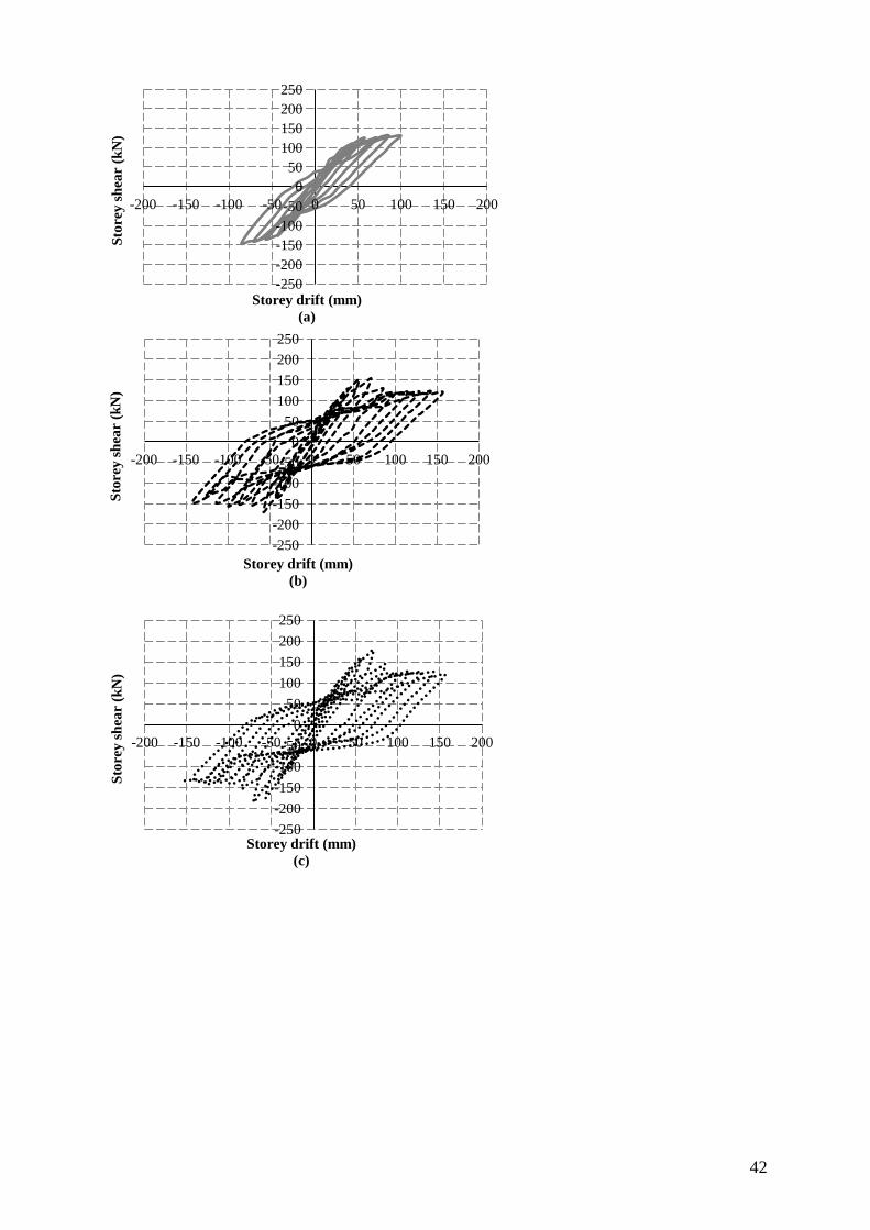
42

-250

-200

-150

-100

-50

0

50

100

150

200

250

-200 -150 -100 -50 0 50 100 150 200

Sto

rey

sh

ear

(kN

)

Storey drift (mm)

(a)

-250

-200

-150

-100

-50

0

50

100

150

200

250

-200 -150 -100 -50 0 50 100 150 200

Sto

rey

sh

ear

(kN

)

Storey drift (mm)

(b)

-250

-200

-150

-100

-50

0

50

100

150

200

250

-200 -150 -100 -50 0 50 100 150 200

Sto

rey

sh

ear

(kN

)

Storey drift (mm)

(c)

43

Vf

(%)

Vy

(kN)

Δy

(mm) Vmax

(kN)

ΔVmax

(mm) Vu

(kN)

Δu

(mm) =

Δu/Δy Vmax/

Vy

CJ 92.4 28.8 143.1 84.3 124.2 140.8 4.90 1.55

0 90.7 28.6 131.8 100 132 100.1 3.50 1.45 1 97.5 28.6 153.7 71.6 118 156.2 5.46 1.58

1.5 98.8 28.6 177.8 71.6 117 156.5 5.47 1.80

2 99.3 28.6 189.9 71.6 112 114.1 3.98 1.91 2.5 99.6 28.6 219.3 100 219 100.2 3.50 2.20

Figure 25: Storey shear-drift hysteresis curves for internal joints with single stirrups and (a) Vf

= 0%, (b) Vf = 1%, (c) Vf = 1.5%, (d) Vf = 2% and (e) Vf = 2.5%

-250

-200

-150

-100

-50

0

50

100

150

200

250

-200 -150 -100 -50 0 50 100 150 200

Sto

rey

sh

ear

(kN

)

Storey drift (mm)

(d)

-250

-200

-150

-100

-50

0

50

100

150

200

250

-150 -100 -50 0 50 100 150

Sto

rey

sh

ear

(kN

)

Storey drift (mm)

(e)

44

-250

-200

-150

-100

-50

0

50

100

150

200

250

-200 -150 -100 -50 0 50 100 150 200

Sto

rey

sh

ear

(kN

)

Storey drift (mm)

(a)

-250

-200

-150

-100

-50

0

50

100

150

200

250

-200 -150 -100 -50 0 50 100 150 200

Sto

rey

sh

ear

(kN

)

Storey drift (mm)

(b)

-250

-200

-150

-100

-50

0

50

100

150

200

250

-200 -150 -100 -50 0 50 100 150 200

Sto

rey

sh

ear

(kN

)

Storey drift (mm)

(c)

-250

-200

-150

-100

-50

0

50

100

150

200

250

-200 -150 -100 -50 0 50 100 150 200

Sto

rey

sh

ear

(kN

)

Storey drift (mm)

(d)

45

Vf (%)

Vy (kN)

Δy

(mm) Vmax (kN)

ΔVmax

(mm) Vu

(kN)

Δu

(mm) =

Δu/Δy Vmax

/ Vy

CJ 92.4 28.8 143.1 84.3 124.2 140.8 4.90 1.55

0 90.2 28.6 129.6 100 128 127.2 4.44 1.44

1 97.8 28.6 154.4 71.6 118 156.2 5.46 1.58

1.5 99.2 28.6 172.5 71.6 121.2 128.7 4.50 1.74

2 100 28.6 193.1 70.4 140 87.55 3.06 1.93

2.5 101 28.6 215.4 85.9 195 100.2 3.50 2.13

Figure 26: Storey shear-drift hysteresis curves for internal joints with SI = 50% and (a) Vf = 0%, (b) Vf = 1%, (c) Vf = 1.5%, (d) Vf = 2% and (e) Vf = 2.5%

-250

-200

-150

-100

-50

0

50

100

150

200

250

-200 -150 -100 -50 0 50 100 150 200

Sto

rey

sh

ear

(kN

)

Storey drift (mm)

(e)

-250

-200

-150

-100

-50

0

50

100

150

200

250

-150 -100 -50 0 50 100 150

Sto

rey

sh

ear

(kN

)

Storey drift (mm)

(a)

-250

-200

-150

-100

-50

0

50

100

150

200

250

-150 -100 -50 0 50 100 150

Sto

rey

sh

ear

(kN

)

Storey drift (mm)

(b)

46

Vf

(%)

Vy

(kN)

Δy

(mm) Vmax

(kN)

ΔVmax

(mm) Vu

(kN)

Δu

(mm) = Δu/Δy Vmax/

Vy

CJ 92.4 28.8 143.1 84.3 124.2 140.8 4.90 1.55

0 89.9 28.6 131.2 100 131 100.1 3.50 1.46

1 93.6 28.6 146.1 71.6 132 114.2 4.00 1.56 1.5 96.5 28.1 158.3 71.6 132 114.4 4.07 1.64

2 98.53 28.1 187.8 73.9 128 114.4 4.07 1.91

2.5 99.25 27.5 214.9 85.9 225.3 114.5 4.16 2.13

Figure 27: Storey shear-drift hysteresis curves for internal joints with SI = 100% and (a) Vf = 0%, (b) Vf = 1%, (c) Vf = 1.5%, (d) Vf = 2% and (e) Vf = 2.5%

-250

-200

-150

-100

-50

0

50

100

150

200

250

-150 -100 -50 0 50 100 150

Sto

rey

sh

ear

(kN

)

Storey drift (mm)

(c)

-250

-200

-150

-100

-50

0

50

100

150

200

250

-150 -100 -50 0 50 100 150

Sto

rey

sh

ear

(kN

)

Storey drift (mm)

(d)

-250

-200

-150

-100

-50

0

50

100

150

200

250

-150 -100 -50 0 50 100 150

Sto

rey

sh

ear

(kN

)

Storey drift (mm)

(e)

47

Figure 28: Variation of storey-shear associated with (a) load carrying capacity and (b) load at

yield (both normalized to control specimen corresponding vales) for different

values of Vf and SI for internal joints

0.8

0.9

1

1.1

1.2

1.3

1.4

1.5

1.6

0 0.5 1 1.5 2 2.5 3

Vm

ax /

Vm

ax,o

Vf (%)

(a)

Single

Stirrup

SI=50%

SI=100%

0.96

0.98

1.00

1.02

1.04

1.06

1.08

1.10

1.12

0 0.5 1 1.5 2 2.5 3

Vy

/ V

y,o

Vf (%)

(b)

Single

Stirrup

SI=50%

SI=100%

48

Figure 29: Variation of (a) ductility ratio and (b) energy absorption (both normalized to

control specimen corresponding vales) for different values of Vf and SI for internal

joints

0.50

0.60

0.70

0.80

0.90

1.00

1.10

1.20

0 0.5 1 1.5 2 2.5 3

µ /

µ,o

Vf (%)

(a)

Single

Stirrup

SI=50%

SI=100%

0

0.2

0.4

0.6

0.8

1

1.2

1.4

1.6

0 0.5 1 1.5 2 2.5 3

Ea

/Ea

,o

Vf (%)

(b)

Single

Stirrup

SI=50%

SI=100%

49

Figure 30: Principal strain contour and vectors for internal joints with SI = 50% and (a) Vf = 0%, (b) Vf = 1%, (c) Vf = 2% taken from storey drift at Δy = 28.6mm

Figure 31: Principal strain contour and vectors for internal joints with SI = 50% and (a) Vf = 0%, (b) Vf = 1%, (c) Vf = 2% taken at Δmax= 69.4mm

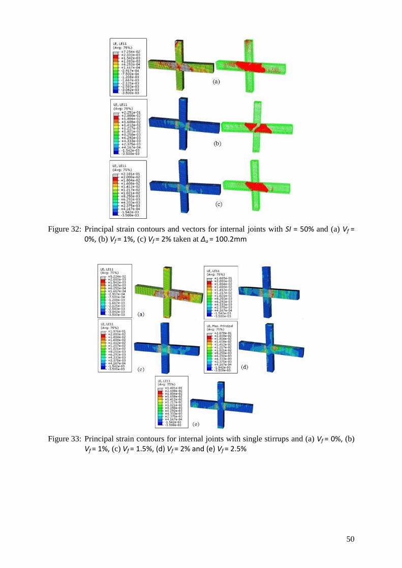
50

Figure 32: Principal strain contours and vectors for internal joints with SI = 50% and (a) Vf = 0%, (b) Vf = 1%, (c) Vf = 2% taken at Δu = 100.2mm

Figure 33: Principal strain contours for internal joints with single stirrups and (a) Vf = 0%, (b)

Vf = 1%, (c) Vf = 1.5%, (d) Vf = 2% and (e) Vf = 2.5%

51

Figure 34: Principal strain contours for internal joints with SI = 50% and (a) Vf = 0%, (b) Vf =

1%, (c) Vf = 1.5%, (d) Vf = 2% and (e) Vf = 2.5%

Figure 35: Principal strain contours for internal joints with SI = 100% and (a) Vf = 0%, (b) Vf = 1%, (c) Vf = 1.5%, (d) Vf = 2% and (e) Vf = 2.5%

52

(a) (b)

Figure 36: Contours showing the variation of (a) ductility ratio and (b) load-carrying

capacity Pmax for different values of rsw and Vf for external joints