15

3.0 SUITABILITY CRITERIA SELECTION, TESTING,AND DEVELOPMENT

3.1 Habitat Suitability Criteria and Species Periodicity

Initially, brook trout, brown trout, white sucker, blacknose dace, and slimy sculpin wereconsidered as possible evaluation species for this study. White sucker, blacknose dace, and slimy sculpinwere considered because they can serve as forage species for trout and frequently occur with trout incoldwater streams. HSC are available for all life stages of white sucker (Twomey and others, 1984).However, white sucker adults are not generally abundant in many of the small headwater trout streamsused in this study. Only a limited number of HSC have been developed for blacknose dace and slimysculpin, and HSC do not exist for all life stages (Sheppard and Johnson, 1984; Mecum, 1984; Trial andothers, 1983). Brook and brown trout are the most recreationally and economically important species inthe study streams. For that reason, only brook and brown trout were used as evaluation species.

Existing brook and brown trout HSC from the following sources were considered for use in thisstudy: Bovee (1978, oral communication, 1994); Aceituno and others (1985); Raleigh and others (1986);Jirka and Homa (1990); Harris and others (1992); Normandeau Associates Inc. (1992); and Gary Whelan,Michigan Department of Natural Resources (oral communication, 1994).

3.1.1 Depth and velocity criteria

The same depth and velocity HSC were used for brook and brown trout, fortransferability testing because the literature indicated very little difference in the criteria for these species.Velocity criteria based on mean water column velocity were used throughout this study. Nose velocityHSC were not used in this study, and were not considered for transferability testing.

The criteria selected for testing are summarized in Table 3.1 and included in Figures3.1-3.8 (pages 44-51). For adults and juveniles, Normandeau Associates’ (1992) depth and velocity HSCwere tested. For spawning, Whelan's (oral communication, 1994) depth and velocity HSC were tested.The spawning life stage includes redd (nest) construction, egg incubation, and immature trout to the timeof emergence from the substrate.

For brook and brown trout fry, Normandeau Associates’ (1992) depth and mean columnvelocity HSC were originally proposed for transferability testing. However, based on generalobservations made in the field, SRBC staff believed the Normandeau HSC for fry would not betransferable to the study streams. The Normandeau HSC indicated a suitability index of 1 (optimum) atwater depths of 1.31 to 1.61 feet. During field investigations, most fry were observed in shallower water,although deeper water was available. Also, the Normandeau HSC indicated that areas with no currentvelocity had a suitability index of 0 (unusable). In the field, many fry were found in areas with little or novelocity. The fry criteria in the literature cited above were reexamined, resulting in the conclusion thatthe Bovee (1978) HSC were more realistic and consistent with the field observations. Bovee's (1978)brown trout fry depth and velocity HSC were used for transferability testing for both brook and browntrout fry.

Tabl

e 3.

1. D

epth

and

Vel

ocity

Hab

itat S

uita

bilit

y C

rite

ria

Use

d fo

r Tr

ansf

erab

ility

Tes

ting

Dep

th H

abita

t Sui

tabi

lity

Cri

teri

aV

eloc

ity H

abita

t Sui

tabi

lity

Cri

teri

aN

orm

ande

au(1

992)

Nor

man

deau

(199

2)W

hela

n(1

994)

Bov

ee(1

978)

Nor

man

deau

(199

2)N

orm

ande

au(1

992)

Whe

lan

(199

4)B

ovee

(197

8)A

dult

Juve

nile

Spa

wni

ngFr

yA

dult

Juve

nile

Spa

wni

ngFr

yD

epth

Inde

xD

epth

Inde

xD

epth

Inde

xD

epth

Inde

xV

eloc

ityIn

dex

Vel

ocity

Inde

xV

eloc

ityIn

dex

Vel

ocity

Inde

xft

ftft

ftft

/sec

ft/s

ecft

/sec

ft/s

ec0

00

00

00.

120.

100

0.21

00.

580

01.

101.

001.

000

0.50

0.12

0.10

0.08

0.40

0.40

0.10

0.70

0.10

0.88

0.10

0.34

1.20

0.94

1.60

0.40

1.00

0.61

0.20

0.22

0.60

0.93

0.50

1.00

0.50

1.00

0.20

0.72

1.65

0.52

2.00

0.80

2.00

0.84

0.30

0.50

0.85

1.00

1.00

0.69

1.00

0.92

0.30

0.84

2.00

0.30

2.60

1.00

3.00

1.00

0.40

0.96

1.70

1.00

1.50

0.50

1.50

0.70

0.60

1.00

2.20

0.20

4.00

1.00

4.00

0.27

0.50

1.00

1.90

0.97

2.40

0.20

2.00

0.26

1.70

1.00

2.50

0.10

7.00

0.21

7.00

0.24

1.10

1.00

2.20

0.80

3.10

0.03

3.50

0.05

3.00

02.

650.

0510

0.00

0.21

8.00

0.08

3.00

1.00

2.50

0.54

5.00

0.03

4.30

03.

000

100.

000.

084.

000

2.70

0.44

6.00

010

0.00

02.

900.

3810

0.00

03.

100.

363.

250.

333.

750.

144.

200.

084.

700.

055.

000

16

17

3.1.2 Substrate/cover criteria

The substrate and cover classification schemes shown in Table 3.2 were used in thisstudy. Combined substrate/cover HSC, that were tested are shown in Table 3.3. Both the classificationscheme and the HSC were based on professional judgment of the investigators. Substrate and covercombinations were identified based on a two-digit coding system. The first digit referred to the substratetype, and the second digit referred to the cover type. Fifteen substrate/cover combinations were thereforepossible. For example, substrate/cover type 1.1 consists of silt or sand with no cover, type 1.2 consists ofsilt or sand with object cover, and so forth.

Table 3.2. Classification Scheme for Substrate and Cover

Substrate Type

1 - Diameter of <3 mm. (silt, sand)2 - Diameter of 3 mm.–64 mm.3 - Diameter of >64 mm.

Cover Type

1 - No cover2 - Object at least 6 inches high and with a cross section horizontal measurement of at

least 1 foot3 - Undercut object along bank4 - Aquatic vegetation5 - Terrestrial vegetation <1 foot above water surface

Table 3.3. Substrate/Cover Habitat Suitability Criteria Used for Transferability Testing

Substrate/Cover Codes

SpawningHSC

FryHSC

JuvenileHSC

AdultHSC

1.1 0 0.5 0.5 0.51.2 0 1 0.8 0.81.3 0 1 1 11.4 0 1 0.8 0.81.5 0 1 0.8 0.82.1 1 0.5 0.5 0.52.2 1 1 0.8 0.82.3 1 1 1 12.4 1 1 0.8 0.82.5 1 1 0.8 0.83.1 0 1 0.8 0.53.2 0 1 0.8 0.83.3 0 1 1 13.4 0 1 0.8 0.83.5 0 1 0.8 0.8

18

3.1.3 Periodicity chart

One important component of the Instream Flow Study is the recognition of specific timeperiods when the various life stages of each species will be present in the study streams, which is calledperiodicity. The periodicity chart, shown in Table 3.4, was developed after reviewing pertinent literatureand discussing brook and brown trout life history information with PFBC and Penn State Universityfisheries biologists.

Table 3.4. Periodicity Chart for Brook and Brown Trout

MonthLife Stage Jan. Feb. Mar. Apr. May June July Aug. Sep. Oct. Nov. Dec.

Adult x x x x x x x x x x x xJuvenile x x x x x x x x x x x xSpawning x x x x xFry x x x x

3.2 Selection of Study Streams for Transferability Testing

Lanka and others (1987) state that trout stream habitat in the Rocky Mountains is greatlyinfluenced by drainage basin geomorphology. Similarly, Nelson and others (1992) found troutdistribution in the North Fork Humboldt River drainage area of northeastern Nevada to be related togeologic district and land type association.

The physical and biological characteristics of reproducing trout streams vary greatly amongphysiographic regions in Pennsylvania, as well as between limestone and freestone streams. No onestream could be selected for HSC modeling that contained all habitat types found in reproducing brookand brown trout streams in the commonwealth. Transferability testing could not be performed for allstudy streams described in section 4.0 because of resource limitations. To evaluate whether the HSCcould be transferred to the study streams, it was assumed that if the HSC could be transferred to onestream in each study region, they also could be transferred to other streams in the same study region. Inthe Ridge and Valley Limestone region, only one stream (Big Spring Creek, Cumberland County) wasidentified that has only a reproducing brook trout population. For that reason, that region and speciescombination was not considered for transferability testing. Therefore, transferability studies wereproposed for one stream from each of the following categories:

• Ridge and Valley Limestone study region, reproducing brown trout stream;• Ridge and Valley Freestone study region, reproducing brown trout stream;• Ridge and Valley Freestone study region, reproducing brook trout stream;• Unglaciated Plateau study region, reproducing brown trout stream; and• Unglaciated Plateau study region, reproducing brook trout stream.

Streams with reproducing trout populations were identified from PFBC data (PFBC, 1993). Thecriteria used for selecting potential streams for transferability testing were a drainage area of less than100 square miles, large numbers of reproducing trout, excellent water quality and visibility, and goodstructural and hydraulic diversity. To facilitate trout identification during sampling, an attempt was madeto select streams that did not contain significant numbers of more than one trout species

19

Field reconnaissance, including electrofishing, was performed in the streams shown in Table 3.5.Results are shown in the table.

Based on the reconnaissance, Elk Creek, Cherry Run, Little Fishing Creek, Young WomansCreek, and Whitehead Run were initially selected as study streams. Both Young Womans Creek and ElkCreek are relatively large streams, compared to the other streams selected. Elk Creek was deleted fromthe study because of limited water clarity and time and cost constraints. Also, a transferability study on asecond large stream would have required more resources than were available.

The study streams finally selected represented the Ridge and Valley Freestone and UnglaciatedPlateau study regions.

All four study sites are located on forested land, and classified by the PFBC as Class A WildTrout Waters. PFBC had not stocked the streams with hatchery trout in recent years.

3.3 Description of Study Streams

3.3.1 Cherry Run

Cherry Run originates from a spring in Bald Eagle State Forest, Hartley Township, UnionCounty, Pa. The stream flows in a southwesterly direction into Centre County, continuing onward in thatdirection until bending towards the southeast to pass through a gap in Paddy Mountain. From the gap, thestream continues in a southeasterly direction, flowing back into Union County and discharging into PennsCreek, about 3.2 miles southwest of Weikert in Hartley Township.

The portion of Cherry Run selected as a study site is about 4 miles long, extending fromthe mouth upstream through Centre County to the Centre-Union County line. The drainage area at thedownstream limit of the study site is 5.9 square miles.

3.3.2 Little Fishing Creek

Little Fishing Creek originates on Nittany Mountain in Bald Eagle State Forest, SpringTownship, Centre County, Pa. The stream flows in a northeasterly direction through Hecla Gap, andenters the Nittany Valley at Mingoville in Walker Township. The stream continues onward in anortheasterly direction into Clinton County, where it discharges into Fishing Creek near Lamar, PorterTownship.

The portion of Little Fishing Creek selected as a study site is about 4.6 miles long, andextends from Hecla Gap upstream above the Greens Valley Road bridge. The drainage area at thedownstream limit of the study site is 5.9 square miles. Although parts of the Little Fishing CreekWatershed are underlain by limestone rocks, this part is underlain by freestone rocks.

3.3.3 Young Womans Creek

Young Womans Creek originates in Sproul State Forest at the confluence of BaldwinBranch and County Line Branch in Chapman Township, Clinton County, Pa. The stream flows in asoutherly direction, entering the West Branch Susquehanna River at North Bend in Chapman Township.The U.S. Geological Survey’s stream gaging station No. 01545600 is located on Young Womans Creek,about 3.7 miles upstream from the mouth and 1.5 miles upstream from Left Branch Young WomansCreek, which is the largest tributary.

Tabl

e 3.

5. S

trea

ms

Con

side

red

for

Tran

sfer

abili

ty S

tudy

Str

eam

Nam

eC

ount

yS

tudy

Reg

ion

Exp

ecte

dTr

out S

peci

esD

ate

Sam

pled

Res

ults

of R

econ

nais

sanc

e S

ampl

ing

Littl

e Fi

shin

g C

reek

Cen

treR

idge

and

Val

ley

Free

ston

eB

rook

May

16,

199

4La

rge

num

bers

of b

rook

trou

t adu

lts, j

uven

iles

and

fry.

Exce

llent

hab

itat d

iver

sity

and

wat

er c

larit

y.El

k C

reek

Cen

treR

idge

and

Val

ley

Lim

esto

neB

row

nM

ay 1

6, 1

994

Larg

e nu

mbe

rs o

f bro

wn

trout

, som

e br

ook

trout

. G

ood

habi

tat d

iver

sity

, lim

ited

wat

er c

larit

y.C

herr

y R

unC

entre

and

Uni

onR

idge

and

Val

ley

Free

ston

eB

row

nM

ay 1

6, 1

994

Man

y ad

ult a

nd ju

veni

le b

row

n tro

ut.

Exce

llent

hab

itat

dive

rsity

and

wat

er c

larit

y.Y

oung

Wom

ans

Cre

ekC

linto

nU

ngla

ciat

ed P

late

auB

row

nM

ay 1

9, 1

994

Larg

e nu

mbe

rs o

f adu

lt an

d ju

veni

le b

row

n tro

ut.

Exce

llent

habi

tat d

iver

sity

and

wat

er c

larit

y.Jo

hn S

umm

erso

n B

ranc

hC

linto

nU

ngla

ciat

ed P

late

auB

rook

May

19,

199

4In

suff

icie

nt n

umbe

rs a

t sam

plin

g si

te n

ear m

outh

. M

ore

abun

dant

ups

tream

acc

ordi

ng to

PFB

C, b

ut a

cces

s to

that

area

was

poo

r.Tr

out R

unC

linto

nU

ngla

ciat

ed P

late

auB

rook

May

19,

199

4In

suff

icie

nt n

umbe

rs o

f fis

h.Lo

st C

reek

Juni

ata

Rid

ge a

nd V

alle

y Fr

eest

one

Bro

wn

June

9, 1

994

Larg

e nu

mbe

rs o

f adu

lt br

own

trout

, rel

ativ

ely

few

juve

nile

san

d fr

y. S

igni

fican

t num

bers

of a

dult

broo

k tro

ut.

Exce

llent

habi

tat d

iver

sity

and

wat

er c

larit

y.W

alla

ce R

unC

entre

Rid

ge a

nd V

alle

y Fr

eest

one

Bro

wn

June

20,

199

4Sm

all n

umbe

rs o

f fis

h. M

ixed

pop

ulat

ion

of a

bout

hal

fbr

ook

and

half

brow

n tro

ut.

Swift

Run

Miff

linR

idge

and

Val

ley

Free

ston

eB

row

nJu

ne 2

0, 1

994

Mix

ed p

opul

atio

n ab

out h

alf b

rook

and

hal

f bro

wn

trout

.G

rove

Run

Cam

eron

Ung

laci

ated

Pla

teau

Bro

okJu

ne 2

1, 1

994

Larg

e nu

mbe

rs o

f bro

ok tr

out,

man

y br

own

trout

.M

onto

ur R

unC

linto

n an

dC

amer

onU

ngla

ciat

ed P

late

auB

rook

June

21,

199

4In

suff

icie

nt n

umbe

rs o

f fis

h.

Whi

tehe

ad R

unC

amer

onU

ngla

ciat

ed P

late

auB

rook

June

21,

199

4La

rge

num

bers

of b

rook

trou

t, ea

sily

acc

essi

ble.

Goo

dha

bita

t div

ersi

ty a

nd w

ater

cla

rity.

A fe

w b

row

n tro

ut.

Laur

el R

unU

nion

Rid

ge a

nd V

alle

y Fr

eest

one

Bro

wn

June

22,

199

4M

ixed

pop

ulat

ion

of b

rook

and

bro

wn

trout

. St

ream

bank

shad

ing

mad

e ob

serv

atio

ns d

iffic

ult.

Lack

awan

na R

iver

Lack

awan

naR

idge

and

Val

ley

Free

ston

eB

row

nJu

ne 2

3, 1

994

Mix

ed p

opul

atio

n of

bro

ok, b

row

n, a

nd ra

inbo

w tr

out.

Goo

d ha

bita

t div

ersi

ty.

Tras

h an

d ho

useh

old

debr

is c

ause

dhe

alth

and

saf

ety

conc

erns

.

20

21

The portion of Young Womans Creek selected as a study site extends from the vicinity ofthe U.S. Geological Survey stream gaging station upstream about 5.2 miles to the vicinity of BeechwoodTrail. The drainage area upstream from the gaging station is 46.2 square miles.

3.3.4 Whitehead Run

Whitehead Run originates in Elk State Forest about 4.3 miles northeast of Cameron inLumber Township, Cameron County, Pa. The stream flows in a westerly direction to meet Hunts Run inLumber Township.

The entire length of Whitehead Run, including its major tributary, Rock Run, wasselected as the study site. The drainage area at the downstream end of the study site is 4.4 square miles.

3.4 Field Data Collection

3.4.1 Procedures

Transferability studies were conducted using the general methodology described byThomas and Bovee (1993). Field work was performed in general accordance with the field manual,which is included as Appendix A of this report. Microhabitat measurements were taken at locationswhere undisturbed fish were observed, and in randomly-selected locations where fish were absent.

Bovee (1986) identified size-class as a good method for classifying groups of fish forHSC development. For the purpose of this investigation, fish less than 2 inches in total length wereconsidered to be fry; fish between 2 and 6 inches long were considered juveniles; and fish 6 or moreinches long were considered adults. This size stratification scheme is consistent with that cited in most ofthe HSC literature listed in section 3.1. Spawning locations were identified by the presence of a totally-or partially-completed redd (nest).

All sampling was performed during daylight hours. Sampling was not performed duringextremely low flows when habitat diversity was limited, or during extremely high flows whenobservations would have been difficult or dangerous. At least one flow measurement was taken near thedownstream end of the sampling area on all trips, except the spawning sampling trip to Cherry Run, whenthe flow was estimated.

Equal areas of all mesohabitat types were sampled, regardless of which mesohabitat typeswere most abundant, or had the greatest concentrations of fish. The locations of all undisturbed fish (orredds) at each mesohabitat sampling site were marked, and appropriate data were recorded.

If two (nonspawning) fish were located within 1 foot of each other, they were consideredto be in the same location (PHABSIM cell), and only one set of microhabitat measurements was taken. Ifa group of fish had individuals less than a foot apart, but the group was spread out over 2 or more feet(which occurred on some occasions with fry), several measurements were made within the occupied areaat locations spaced a foot apart. Sampling for adults, juveniles, and fry was generally performed by athree-person crew. However, a four-person crew was used on a few of the juvenile and adult samplingtrips, allowing two crew members to simultaneously make microhabitat measurements, and thereby speedup the data collection process. A two-person crew was used for all field trips involving spawning adultfish.

22

Snorkel gear, surface observations, and electrofishing were used to observe fish locations,which were documented. When identifying fish locations, a conscious effort was made to avoid fishfright and investigator bias.

The effectiveness of using snorkel gear to make direct underwater observations ofundisturbed fish has been well documented (Bovee, 1986; Bovee and Zuboy, 1988). For this reason,snorkel gear was used to the maximum extent possible in making in-situ observations of adults, juveniles,and fry for the transferability studies. Snorkel gear was used extensively, and was the preferred means ofidentifying adult, juvenile, and fry locations in Young Womans Creek. However, the method could notbe effectively used in Whitehead Run and Cherry Run, because nearly all of the sampling area were tooshallow to sample with snorkel gear. For the same reason, snorkel gear could not be effectively used tosample adult and juvenile locations in Little Fishing Creek, but was used to a limited extent to sample frylocations in pool habitat during higher water conditions. For habitat types that could not be effectivelysampled with snorkel gear, surface observations and electrofishing were used to identify fish locations.

When making observations with snorkel gear, the diver used his hands and legs to pull orpush quietly along the bottom, moving systematically in an upstream direction to identify the locations ofundisturbed fish. In deep water and in areas with extremely fast current, the diver pulled himself throughthe study reach on a rope, which had been previously anchored.

Surface observations were used in clear, shallow water to locate fish or redds at eachmesohabitat sampling site. Because of low flow conditions and excellent water clarity, surfaceobservations were the only means used to identify spawning locations. The observer wore drab orcamouflage clothing, and made a cautious approach in an upstream direction through the sampling area,taking care not to frighten fish. Surface observations were generally made with the aid of polarizedsunglasses. In some instances, binoculars also were used to assist in making surface observations.

Electrofishing was generally performed with a backpack DC shocker and two hand-heldelectrodes. However, an AC shocker was used on one of the adult/juvenile sampling trips to Cherry Run,due to equipment malfunction. A rat-tail probe was used as one of the electrodes when sampling fry onall streams, except Young Womans Creek, because of equipment problems. For each point sampled, theelectrodes were carefully positioned, the electrical current was then activated, and the locations of fishidentified. If necessary, fish were collected with a dipnet for identification or measurement. All collectedfish were returned to the stream.

Fish and redd locations were marked with a lead fishing sinker, to which a numberedpiece of plastic surveyor's tape was attached. The date, time, mesohabitat type, observation technique,marker tag number, species, length, and life stage were recorded. A copy of the field data sheets used foroccupied locations is shown as Appendix 3 of the field manual for HSC transferability testing.

After fish and redd locations were marked, water depth was measured and recorded to thenearest 0.01 foot, using a top-setting rod equipped with a current meter. The number of cup rotations perunit of time was recorded on the data sheet so that mean current velocity for each location could becalculated. Where the water depth was less than 2.5 feet, one current meter reading was taken at six-tenths of the distance from the water surface to the stream bottom. Where the water depth was greaterthan 2.5 feet, one current meter reading was taken at two-tenths and another reading was taken at eight-tenths of the distance from the water surface to the stream bottom. The results of the two velocities wereaveraged. Water temperature in degrees Celsius was periodically measured and recorded.

23

Before removing the fish location markers from the stream bottom, a random samplingprocedure was used to select locations that were unoccupied by fish. The procedure is described inAppendix A.

Unoccupied locations were not selected within 1 foot of an occupied location. Data werecollected and recorded on a copy of the field data sheet for unoccupied locations, shown as Appendix 4 ofthe field manual.

The dates of field observations and a record of streamflow measurements are shown inTable 3.6. Relatively large variations in streamflow occurred in Young Womans Creek due to rain andthunderstorm activity. On some occasions, sampling had to be delayed until water clarity improved andstream conditions stabilized. Under these circumstances, care was taken to avoid delays in takingmicrohabitat measurements after occupied and unoccupied locations were identified, because of changingflow conditions.

3.4.2 General observations

Young Womans Creek was ideally suited for use of snorkel gear. Excellent water claritynormally allowed a diver to spot adult fish that were more than 20 feet away, if they were approachedcautiously by moving in an upstream direction. The tendency of fish to remain in position whenapproached by a diver varied with the life stage, water conditions, current velocity, and cover being usedby the fish and diver at the time of observation. In general, adult fish were more difficult to approachthan juveniles, and juveniles were more difficult to approach than fry. As a general rule, adult fish inopen, moving water could be approached to within about 10 feet before showing fright reactions (ceasingto feed on drifting material, making jerky or tense body movements, preparing to dart away, graduallymoving away from the diver, etc.). When cover was available, adult trout could be approached even moreclosely. Some large brown trout resting under rock ledges could almost be touched by the diver. Manyjuveniles continued to feed when only a few feet from the diver, and some fry could be approached towithin inches of the face mask.

Initially, only brown trout data were collected when sampling for adults and juveniles inYoung Womans Creek. However, both brook trout and brown trout were observed in the stream. Duringthe second field visit, microhabitat data were collected for both species.

In Young Womans Creek, positive species identification of undisturbed adults andjuveniles was an easy matter because of excellent underwater visibility, the magnification effect causedby looking through the diver’s mask, and the fact that fish were moving naturally with fins spread andmarkings easily visible. Species identification of fry was dependent on being able to see a dark spot onthe adipose fin of brook trout. This spot is not present on brown trout. Eighty-nine fry locations weresampled in Young Womans Creek. However, because of the small size of the fry (0.75 to 1.25 inches)and the fact that many of the smaller fish were heavily pigmented, field identification to the species levelwas not always possible. Thirty-three of the fry from these locations were identified as brook trout, 14were identified as brown trout, and 42 could not be accurately identified.

In Young Womans Creek, brook trout seemed to be more commonly associated with poolhabitat, while brown trout appeared to be more closely associated with cover. Brown trout were moreabundant in the lower region of the study area (in the vicinity of the U.S. Geological Survey gagingstation). Brook trout were more abundant in upstream areas (from Bull Run upstream to the vicinity ofBeechwood Trail).

Tabl

e 3.

6. S

ampl

ing

Dat

es a

nd S

trea

mflo

w M

easu

rem

ents

Type

of F

ish/

Dat

es S

ampl

ed a

nd S

trea

mflo

wC

herr

y R

unLi

ttle

Fis

hing

Cre

ekY

oung

Wom

ans

Cre

ekW

hite

head

Run

Adu

lt/Ju

veni

le S

ampl

ing,

Fir

st D

ata

Set

Dat

es S

ampl

edJu

ly 2

5-27

, 199

4Ju

ly 1

1-13

, 199

4Ju

ly 6

,7,8

,13,

& 1

4, 1

994

July

18-

20, 1

994

July

20-

21, 1

994

Aug

ust 8

-9, 1

994

Stre

amflo

w1.

68 c

fs (J

uly

25, 1

994)

1.54

cfs

(Jul

y 11

, 199

4)11

0 cf

s (J

uly

6, 1

994)

4.84

cfs

(Jul

y 20

, 199

4)

80

cfs

(Jul

y 7,

199

4)

47

cfs

(Jul

y 13

, 199

4)

45

cfs

(Aug

ust 8

, 199

4)A

dult/

Juve

nile

Sam

plin

g, S

econ

d D

ata

Set

Dat

es S

ampl

edA

ugus

t 22-

25, 1

994

Sept

embe

r 6-8

, 199

4A

ugus

t 10-

11, 1

994

Aug

ust 2

9-31

, 199

4A

ugus

t 15-

17, 1

994

Sept

embe

r 1, 1

994

Stre

amflo

w5.

90 c

fs (A

ugus

t 23,

199

4)2.

80 c

fs (S

epte

mbe

r 8, 1

994)

36

cfs

(A

ugus

t 10,

199

4)9.

58 c

fs (S

epte

mbe

r 1, 1

994)

31

cfs

(A

ugus

t 11,

199

4)21

9 cf

s (A

ugus

t 15,

199

4)18

6 cf

s (A

ugus

t 16,

199

4)15

3 cf

s (A

ugus

t 17,

199

4)Sp

awni

ng S

ampl

ing

Dat

es S

ampl

edN

ovem

ber 3

-4, 1

994

Oct

ober

18-

21, 1

994

Oct

ober

24-

26, 1

994

Oct

ober

10-

14, 1

994

Nov

embe

r 7-8

, 199

4St

ream

flow

4 cf

s (e

stim

ated

)2.

21 c

fs (O

ctob

er 2

1, 1

994)

1

2 cf

s (O

ctob

er 2

4, 1

994)

0.78

cfs

(Oct

ober

14,

199

4)F

ry S

ampl

ing

Dat

es S

ampl

edA

pril

17-1

9, 1

995

Apr

il 24

-26,

199

5M

ay 8

-11,

199

5M

ay 1

-3, 1

995

Stre

amflo

w6.

73 c

fs (A

pril

19, 1

995)

8.15

cfs

(Apr

il 24

, 199

5)

27 c

fs (

May

8, 1

995)

2.20

cfs

(May

3, 1

995)

26

cfs

(M

ay 1

0, 1

995)

156

cfs

(May

11,

199

5)

24

25

During all of the field trips to Little Fishing Creek, the only species of trout observed wasbrook trout. Some brown trout were observed during the fall in the lower portion of Whitehead Run, butthe predominant species present was brook trout. The predominant species present in Cherry Run wasbrown trout, although some brook and rainbow trout also were observed.

When identifying redd locations, it was important to look very carefully for gravel thathad been disturbed. In many cases, the pit (depression) and tailspill (downstream area of loose gravel) ofredds were difficult to identify, especially if the redd was small and not recently constructed. Becausesmall brook trout make small redds, it was necessary to look carefully in even small pockets of gravel.The tailspills for some redds were only slightly larger than the 6- or 7-inch long fish that made them.Larger fish made larger redds, and some brown trout redds in Young Womans Creek were found withtailspills that were more than a foot long. Redds were frequently found in the tails of pools, but they werefound in all mesohabitat types (riffles, runs, and pools).

As recommended by Dr. Robert Carline of Penn State University, field crews used awalking stick to poke into potential redd locations to determine if the sediments were loose and may havebeen excavated by trout. It was often possible to dislodge eggs to confirm the site was, in fact, a redd bydigging with the stick to a depth of several inches (depending on the size of the redd). Crews initially duginto the bottom sediments by hand to confirm redd locations, and used a fine-meshed screen colander tocatch dislodged eggs. However, digging with a walking stick was just as effective, and was much lessdamaging to redds.

Redds were much easier to identify with good lighting (such as during the middle of asunny day) and when there was little or no wind to create a surface disturbance on the water. Most reddswere found in relatively flat, shallow water. However, some were found in areas with almost no flow,and a few were found in relatively choppy water. Side channels seemed to be especially productivelocations, probably because flow was reduced and gravel was more abundant in many of these areas.Redds were more easily identified when they were occupied by fish.

Although brown trout were actively constructing redds when Cherry Run was sampledfor spawning, no eggs were recovered from redd locations. For this reason, it was assumed that samplinghad been conducted at the beginning of the spawning period.

Eggs were recovered from redds on all three of the other streams sampled. Based on theappearance of redds and the activity of fish, sampling was conducted somewhat after the peak spawningactivity on Little Fishing Creek and Whitehead Run. Many brown trout were found occupying redds inYoung Womans Creek, indicating sampling probably occurred during the time of peak spawning activity.Although a few brook trout also were seen on redds in Young Womans Creek, the majority of reddsobserved in that stream were made by brown trout.

3.5 Transferability Study Data Analysis Procedures

Field data were used to perform transferability testing of HSC in accordance with the procedurescited by Thomas and Bovee (1993). The number of occupied and unoccupied sites (cells) havingoptimum usable, suitable, and unsuitable habitat were calculated for the appropriate study streams,species, and life stages. For this test, optimum habitat was assumed to have a suitability index of 0.8 ormore, and suitable habitat was assumed to have a suitability index of 0.1 or more (Bovee, oralcommunication, 1994). One-sided chi-square tests (alpha = .05) were performed using the formula shownbelow.

26

T = N ad bc

a b c d a c b d

( )

( )( ( )( )

−

+ + + +

where: T = the test statistica = the number of occupied optimum (or suitable) cells;b = the number of occupied usable (or unsuitable) cells;c = the number of unoccupied optimum (or suitable) cells;d = the number of unoccupied usable (or unsuitable) cells; andN = the total number of cells.

To be considered transferable, the test statistic had to be greater than 1.6449.

For the purpose of data analysis, all redds observed in Young Womans Creek were assumed to bebrown trout redds, unless brook trout were observed at a particular redd location. Insufficient brook troutredds were observed to warrant use of data from these redds for transferability testing.

Brook, brown, and unidentified fry data from Young Womans Creek were considered collectivelyfor the purpose of transferability testing.

3.6. Transferability Study Data Analysis Results

Transferability testing indicated the HSC discussed in section 3.1 were not transferable to most ofthe streams tested. The results of transferability testing are summarized in Table 3.7. Chi-square testresults used in compiling Table 3.7 are shown in Appendix B.

Table 3.7. Results of Transferability Testing

Stream and Species Life Stage Transferable?Cherry Run, Brown Trout Adult No

Juvenile NoSpawning NoFry No

Little Fishing Creek, Brook Trout Adult NoJuvenile NoSpawning NoFry No

Young Womans Creek, Brown Trout Adult YesJuvenile NoSpawning NoFry (Brook and Brown) No

Young Womans Creek, Brook Trout Adult YesJuvenile No

Whitehead Run, Brook Trout Adult NoJuvenile NoSpawning NoFry No

27

3.7 Criteria Development

3.7.1 Procedures

Because only a few of the HSC were transferable, the following options were considered:

1. Collect additional data and develop new HSC for testing;2. Test other existing HSC;3. Modify the HSC and rerun the transferability test; and4. Develop new criteria from data already collected.

Option 1 would have been the most desirable, if additional time and funds had beenavailable. Development of individual sets of new criteria for each of the transferability study streamswould have required about four times as much work as the transferability testing that had already beenperformed. Therefore, new criteria were developed based on the data available from the transferabilitystudies. All the data collected for each species and/or life stage were pooled to develop the new HSC.

Prior to developing the new criteria, histograms were prepared of the occupied andunoccupied site data used for transferability testing. Additional HSC were identified and comparedvisually to the histograms to see whether there was a match. Since there was no match, the modifiedforage index and the linear index, described by Schreck and Moyle (1990), were both used in a systematicapproach to developing new HSC.

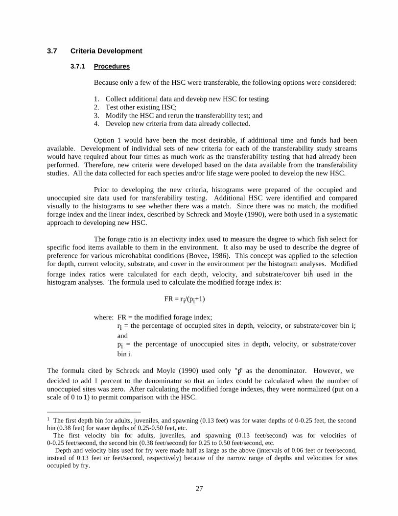
The forage ratio is an electivity index used to measure the degree to which fish select forspecific food items available to them in the environment. It also may be used to describe the degree ofpreference for various microhabitat conditions (Bovee, 1986). This concept was applied to the selectionfor depth, current velocity, substrate, and cover in the environment per the histogram analyses. Modifiedforage index ratios were calculated for each depth, velocity, and substrate/cover bin1 used in thehistogram analyses. The formula used to calculate the modified forage index is:

FR = ri/(pi+1)

where: FR = the modified forage index;ri = the percentage of occupied sites in depth, velocity, or substrate/cover bin i;andpi = the percentage of unoccupied sites in depth, velocity, or substrate/coverbin i.

The formula cited by Schreck and Moyle (1990) used only "pi" as the denominator. However, wedecided to add 1 percent to the denominator so that an index could be calculated when the number ofunoccupied sites was zero. After calculating the modified forage indexes, they were normalized (put on ascale of 0 to 1) to permit comparison with the HSC.

1 The first depth bin for adults, juveniles, and spawning (0.13 feet) was for water depths of 0-0.25 feet, the secondbin (0.38 feet) for water depths of 0.25-0.50 feet, etc. The first velocity bin for adults, juveniles, and spawning (0.13 feet/second) was for velocities of0-0.25 feet/second, the second bin (0.38 feet/second) for 0.25 to 0.50 feet/second, etc. Depth and velocity bins used for fry were made half as large as the above (intervals of 0.06 feet or feet/second,instead of 0.13 feet or feet/second, respectively) because of the narrow range of depths and velocities for sitesoccupied by fry.

28

The linear food index was first proposed by Strauss (1979) and is

L = ri - pi

where: L = the linear index, and ri and pi are as defined above.

The modified forage index always has positive values. However, values for the linearindex range from -1 to +1, with positive values indicating preference and negative values indicatingavoidance. No attempt was made to normalize the linear indexes.

3.7.2 Depth and velocity criteria

Normalized modified forage indexes (NMFIs) for depth and velocity for each life stageand stream were plotted on the same graphs as the depth and velocity HSC used for transferability testing,and are shown as Figures 3.1 through 3.8.

Brook trout NMFIs for Little Fishing Creek, Whitehead Run, and Young Womans Creekwere used to develop new adult and juvenile brook trout HSC. Brown trout NMFIs for Young WomansCreek and Cherry Run were used to develop new adult and juvenile brown trout HSC.

New HSC for spawning brook trout were developed using NMFIs for Little FishingCreek and Whitehead Run. New HSC for spawning brown trout were developed from NMFIs for YoungWomans Creek and Cherry Run.

Because of the close similarity of fry NMFIs for all four streams, new HSC for fry weredeveloped from data collected from all four streams, and brook and brown trout fry HSC were consideredidentical.

When developing new depth and velocity HSC using data from several streams, the datapoint with the higher NMFI from each bin was generally used. The new HSC may, therefore, beconsidered conservative because they encompass data from all of the streams considered. If a questionarose regarding a particular data point (such as a modified forage index calculated from relatively few fishobservances), the linear index also was considered in developing the new HSC.

The NMFI for fry depth in Whitehead Run (Figure 3.4) is a value of 1 at depths of0.94 feet and 1.19 feet. This produced an unusual peak in the graph for Whitehead Run that was muchdifferent from peaks in the graphs for the other streams. Because of the small number (2 out of 57) of fryobservations made at the above depths in Whitehead Run, these data points were not used to construct therevised criteria, and the depth with the next highest NMFI (0.56 ft.) was considered to have a suitabilityindex of 1.

3.7.3 Substrate and cover

Prior to constructing new substrate/cover HSC, modified forage indexes were calculatedfor all 15 combined substrate/cover categories. Modified forage indexes also were calculatedindependently for all three substrate types and for all five cover types. The independently calculatedsubstrate and cover modified forage indexes were most easily analyzed and were used to develop newHSC. The NMFIs used to develop new substrate/cover HSC are shown in Table 3.8.

Fig

ure

3.1.

Adu

lt N

orm

aliz

ed M

odifi

ed F

orag

e In

dexe

s fo

r D

epth

0.0

0.1

0.2

0.3

0.4

0.5

0.6

0.7

0.8

0.9

1.0 0.

130.

380.

630.

881.

131.

381.

631.

882.

132.

382.

632.

883.

133.

383.

633.

884.

134.

384.

634.

885.

13

DE

PTH

(ft)

INDEXLi

ttle

Fish

ing

(Bro

ok)

You

ng W

oman

s (B

row

n)Y

oung

Wom

ans

(Bro

ok)

Whi

tehe

ad R

un (B

rook

)C

herry

Run

(Bro

wn)

Nor

man

deau

(199

2) H

SC

29

Fig

ure

3.2.

Juv

enile

Nor

mal

ized

Mod

ified

For

age

Inde

xes

for

Dep

th

0.0

0.1

0.2

0.3

0.4

0.5

0.6

0.7

0.8

0.9

1.0

0.13

0.38

0.63

0.88

1.13

1.38

1.63

1.88

2.13

2.38

2.63

2.88

3.13

3.38

3.63

3.88

4.13

4.38

4.63

4.88

5.13

DE

PTH

(ft)

INDEXLi

ttle

Fish

ing

(Bro

ok)

You

ng W

oman

s (B

row

n)Y

oung

Wom

ans

(Bro

ok)

Whi

tehe

ad R

un (B

rook

)C

herry

Run

(Bro

wn)

Nor

man

deau

(199

2) H

SC

30

Fig

ure

3.3.

Spa

wni

ng N

orm

aliz

ed M

odifi

ed F

orag

e In

dexe

s fo

r D

epth

0.0

0.1

0.2

0.3

0.4

0.5

0.6

0.7

0.8

0.9

1.0

0.13

0.38

0.63

0.88

1.13

1.38

1.63

1.88

2.13

2.38

2.63

2.88

3.13

3.38

3.63

3.88

4.13

4.38

4.63

4.88

5.13

5.38

5.63

5.88

6.13

6.38

6.63

6.88

7.13

DE

PTH

(ft)

INDEXL

ittl

e F

ish

ing

(Bro

ok)

Yo

ung

Wo

ma

ns

(Bro

wn

)W

hit

ehea

d R

un (

Bro

ok)

Ch

erry

Run

(B

row

n)

Wh

elan

(19

94

) H

SC

31

Fig

ure

3.4.

Fry

Nor

mal

ized

Mod

ified

For

age

Inde

xes

for

Dep

th

0.0

0.1

0.2

0.3

0.4

0.5

0.6

0.7

0.8

0.9

1.0

0.06

0.19

0.31

0.44

0.56

0.69

0.81

0.94

1.06

1.19

1.31

1.44

1.56

1.69

1.81

1.94

2.06

2.19

2.31

2.44

2.56

2.69

2.81

2.94

3.06

3.19

3.31

3.44

3.56

3.69

3.81

3.94

4.06

4.19

4.31

4.44

4.56

4.69

4.81

4.94

5.06

5.19

DE

PTH

(ft)

INDEX

Littl

e Fi

shin

g (B

rook

)Y

oung

Wom

ans

(Bot

h)W

hite

head

Run

(Bro

ok)

Che

rry

Run

(Bro

wn)

Bov

ee (1

978)

HS

C

32

Fig

ure

3.5.

Adu

lt N

orm

aliz

ed M

odifi

ed F

orag

e In

dexe

s fo

r V

eloc

ity

0.0

0.1

0.2

0.3

0.4

0.5

0.6

0.7

0.8

0.9

1.0

0.13

0.38

0.63

0.88

1.13

1.38

1.63

1.88

2.13

2.38

2.63

2.88

3.13

3.38

3.63

3.88

4.13

4.38

4.63

4.88

5.13

5.38

5.63

5.88

VE

LOC

ITY

(ft/s

ec)

INDEXLi

ttle

Fish

ing

(Bro

ok)

You

ng W

oman

s (B

row

n)Y

oung

Wom

ans

(Bro

ok)

Whi

tehe

ad R

un (B

rook

)C

herr

y R

un (B

row

n)N

orm

ande

au (1

992)

HS

C

33

Fig

ure

3.6.

Juv

enile

Nor

mal

ized

Mod

ified

For

age

Inde

xes

for

Vel

ocity

0.0

0.1

0.2

0.3

0.4

0.5

0.6

0.7

0.8

0.9

1.0

0.13

0.38

0.63

0.88

1.13

1.38

1.63

1.88

2.13

2.38

2.63

2.88

3.13

3.38

3.63

3.88

4.13

4.38

4.63

4.88

5.13

5.38

5.63

5.88

VE

LOC

ITY

(ft/s

ec)

INDEXLi

ttle

Fish

ing

(Bro

ok)

You

ng W

oman

s (B

row

n)Y

oung

Wom

ans

(Bro

ok)

Whi

tehe

ad R

un (

Bro

ok)

Che

rry

Run

(Bro

wn)

Nor

man

deau

(199

2) H

SC

34

Fig

ure

3.7.

Spa

wni

ng N

orm

aliz

ed M

odifi

ed F

orag

e In

dexe

s fo

r V

eloc

ity

0.0

0.1

0.2

0.3

0.4

0.5

0.6

0.7

0.8

0.9

1.0

0.13

0.38

0.63

0.88

1.13

1.38

1.63

1.88

2.13

2.38

2.63

2.88

3.13

3.38

3.63

3.88

4.13

4.38

VE

LOC

ITY

(ft/s

ec)

INDEXLi

ttle

Fish

ing

(Bro

ok)

You

ng W

oman

s (B

row

n)W

hite

head

Run

(Bro

ok)

Che

rry

Run

(Bro

wn)

Whe

lan

(199

4) H

SC

35

Fig

ure

3.8.

Fry

Nor

mal

ized

Mod

ified

For

age

Inde

xes

for

Vel

ocity

0

0.1

0.2

0.3

0.4

0.5

0.6

0.7

0.8

0.91

0.06

0.19

0.31

0.44

0.56

0.69

0.81

0.94

1.06

1.19

1.31

1.44

1.56

1.69

1.81

1.94

2.06

2.19

2.31

2.44

2.56

2.69

2.81

2.94

3.06

3.19

3.31

3.44

3.56

3.69

3.81

3.94

4.06

VE

LOC

ITY

(ft/

sec)

INDEX

Littl

e Fi

shin

g(B

rook

)Y

oung

Wom

ans(

Bro

wn)

Whi

tehd

Run

(Bro

ok)

Che

rry

Run

(Bro

wn)

Whe

lan

(199

4)H

SC

36

Tabl

e 3.

8. N

orm

aliz

ed M

odifi

ed F

orag

e In

dexe

s fo

r Su

bstr

ate

and

Cov

er

Type

of F

ish/

Sub

stra

te T

ype

Cov

er T

ype

Nam

e of

Str

eam

12

31

23

45

Adu

lt B

rook

Tro

utLi

ttle

Fish

ing

Cre

ek1

0.2

0.6

00.

51

00.

3Y

oung

Wom

ans

Cre

ek0

10.

70.

80.

81

00

Whi

tehe

ad R

un1

0.4

0.5

00.

61

00

Adu

lt B

row

n Tr

out

You

ng W

oman

s C

reek

0.9

0.6

10.

10.

21

0.2

0C

herr

y R

un0.

50.

41

0.1

0.4

10.

20

Juve

nile

Bro

ok T

rout

Littl

e Fi

shin

g C

reek

10.

60.

80.

10.

41

0.2

0.5

You

ng W

oman

s C

reek

10.

10

0.3

0.2

10.

40

Whi

tehe

ad R

un1

0.6

0.6

01

0.9

00.

1Ju

veni

le B

row

n Tr

out

You

ng W

oman

s C

reek

0.6

10.

80.

10.

31

0.2

0.1

Che

rry

Run

0.2

0.7

10.

30.

81

0.8

0Sp

awni

ng B

rook

Tro

utLi

ttle

Fish

ing

Cre

ek0

10

0.1

0.1

10

0.1

Whi

tehe

ad R

un0.

21

00.

30.

61

00.

5Sp

awni

ng B

row

n Tr

out

You

ng W

oman

s C

reek

01

00.

10

10.

20

Che

rry

Run

01

0.1

0.6

0.2

10.

10

Fry

(Bro

ok/B

row

n Tr

out C

ombi

ned)

Littl

e Fi

shin

g C

reek

10.

30.

10.

40.

30.

80

1W

hite

head

Run

10.

10.

10.

50.

80.

51

0Y

oung

Wom

ans

Cre

ek1

0.6

0.1

0.1

0.2

0.1

01

Che

rry

Run

10.

40.

10.

60.

41

00

Not

e: S

ubst

rate

and

cov

er ty

pe a

re d

efin

ed in

Tab

le 3

.2.

37

38

When cover and substrate were analyzed independently, adult brook trout appeared toshow strong preference for cover, but little preference for substrate type. Adult brook trout NMFIs forsubstrate type 1 (silt) ranged from a value of 1 in Little Fishing Creek and Whitehead Run to a value of 0in Young Womans Creek. The apparent explanation for this difference is that substrate type isunimportant, compared to cover type for the adult life stage. Because no definite pattern could beidentified with respect to substrate preference, new adult brook trout substrate/cover HSC were developedbased entirely on cover type.

Adult brook trout NMFIs for cover type 1 (no cover) were 0 for both Little Fishing Creekand Whitehead Run. For this reason, cover type 1 was assigned a suitability index of 0 for adult brooktrout. Therefore, substrate/cover codes 1.1, 2.1, and 3.1 also were given HSC values of 0. Although theadult brook trout NMFI for cover type 1 in Young Womans Creek was 0.8, this value was not used fornew HSC development because adult brown trout appeared to be competing with adult brook trout forcover in this stream. It appears that adult brook trout were being forced into the “no cover” situation as aresult of this competition. Brown trout were not found in the section sampled in Little Fishing Creek, andwere found in limited numbers in only some parts of Whitehead Run. In Young Womans Creek, adultbrown trout seemed to be more closely associated with cover, while adult brook trout appeared to be moreclosely associated with pool habitat. Adult brook trout would probably have made more extensive use ofcover on Young Womans Creek if much of the cover had not already been occupied by adult brown trout.

Adult brook trout NMFIs for cover type 2 (object at least 6 inches high, and with a cross-section horizontal measurement of at least 1 foot) were 0.5 for Little Fishing Creek and 0.6 for WhiteheadRun. Therefore, a suitability index of 0.6 was assigned to cover type 2 for adult brook trout. Althoughthe adult brook trout NMFI for cover type 2 in Young Womans Creek was 0.8, this value was not used forHSC development because of possible effects of competition between brook and brown trout previouslycited. Selection of the higher value was consistent with the approach used in modifying depth andvelocity HSC, as described above.

Cover type 3 (undercut object along bank) had an NMFI of 1 for adult brook trout on allof the streams tested, and was assigned a suitability index of 1.

Only a limited amount of adult brook trout data for cover types 4 (aquatic vegetation) and5 (terrestrial vegetation less than 1 foot above water surface) were available for the streams sampled.However, if these cover types had been present, adult brook trout probably would have used them inmuch the same way that they used cover type 2 (object cover). For this reason, the suitability index valueassigned to brook trout adults for cover type 2 also was assigned to cover types 4 and 5.

Adult brown trout also appeared to show strong preferences for cover and not forsubstrate type. Therefore, new adult brown trout substrate/cover HSC also were developed, based solelyon cover type. Adult brown trout NMFIs for cover type 1 (no cover) were 0.1 for both Young WomansCreek and Cherry Run. For this reason, cover type 1 was assigned a suitability index of 0.1 for adultbrown trout. Adult brown trout NMFIs for cover type 2 (object cover) were 0.2 for Young WomansCreek and 0.4 for Cherry Run. Therefore, a suitability index of 0.4 was assigned to cover type 2 for adultbrown trout. Cover type 3 (undercut object along bank) had an NMFI of 1 for adult brown trout in bothYoung Womans Creek and Cherry Run, and was assigned a suitability index of 1. Cover types 4 (aquaticvegetation) and 5 (terrestrial vegetation less than 1 foot above water surface) were uncommon. Becausethese are types of object cover, they were given the same HSC values as cover type 2 (object cover) forbrown trout.

As with adults, juvenile brook trout did not appear to show preferences for substrate type,and new substrate/cover HSC were developed based entirely on cover type. Juvenile brook trout NMFIs

39

for cover type 1 (no cover) were 0.1 for Little Fishing Creek, 0.3 for Young Womans Creek, and 0 forWhitehead Run. Cover type 1 was assigned a suitability index of 0.3 for juvenile brook trout based on theYoung Womans Creek value. Although there appeared to be competition between brook and brown troutadults for available cover in Young Womans Creek, it did not appear to be an important factor forjuveniles, because both species appeared to use the available habitat in a similar manner.

Juvenile brook trout NMFIs for cover type 2 (object cover) were 0.4 for Little FishingCreek, 0.2 for Young Womans Creek, and 1 for Whitehead Run. A suitability index of 1 was assigned tocover type 2 for juvenile brook trout. Cover type 3 (undercut object along bank) had an NMFI of 1 forjuvenile brook trout in Little Fishing Creek and Young Womans Creek, and a value of 0.9 for juvenilebrook trout in Whitehead Run. Cover type 3 was assigned a suitability index of 1 for juvenile brook trout.As described above for brook trout adults, only a limited amount of juvenile brook trout data wereavailable for cover types 4 (aquatic vegetation) and 5 (terrestrial vegetation less than 1 foot above watersurface), and these cover types were given the same suitability index values as cover type 2 for juvenilebrook trout.

New juvenile brown trout substrate/cover HSC also were developed, based entirely oncover type. Juvenile brown trout NMFIs for cover type 1 (no cover) were 0.1 for Young Womans Creek,and 0.3 for Cherry Run. Cover type 1 was assigned a suitability index of 0.3 for juvenile brown trout.

Juvenile brown trout NMFIs for cover type 2 (object cover) were 0.3 for Young WomansCreek, and 0.8 for Cherry Run. A suitability index of 0.8 was assigned to cover type 2 for juvenile browntrout. Cover type 3 (undercut object along bank) had an NMFI of 1 for juvenile brown trout for both ofthe streams sampled. Cover type 3 was assigned a suitability index of 1 for juvenile brown trout. Only alimited amount of juvenile brown trout data were available for cover types 4 (aquatic vegetation) and 5(terrestrial vegetation less than 1 foot above water surface), and these cover types were given the samesuitability index values as cover type 2 for juvenile brown trout.

Based on the data for occupied sites, cover appeared to be unimportant for spawningbrook trout and brown trout, but substrate was extremely important. Substrate type 2 (coarse sand/gravel)had an NMFI of 1 on all four streams, and was given a suitability index of 1 for both brook and browntrout. Substrate types 1 (silt/fine sand) and 3 (pebbles and larger) were used to a much lesser extent byboth species. However, substrate type 1 had an NMFI of 0.2 for Whitehead Run, and therefore, wasgiven a suitability index of 0.2 for brook trout. Substrate type 3 had an NMFI of 0.1 in Cherry Run, andtherefore, was given a suitability index of 0.1 for brown trout.

When NMFIs for fry substrate and cover were analyzed separately, substrate wasimportant, but cover usually did not appear to be. Although fry were found in association with cover type5 (terrestrial vegetation less than 1 foot above water surface) where it was available on Young WomansCreek and Little Fishing Creek, fry may have been selecting more for low velocity water near shore,rather than specifically for cover type 5, which had an NMFI of 1 for both of these streams. Cover type 5was not present at any of the occupied or unoccupied fry sampling sites on Whitehead Run or CherryRun. Cover type 5 was assigned a suitability index of 1 in association with all substrate types.

For fry, substrate type 1 (silt/fine sand) had an NMFI of 1 for all four streams. Thissubstrate was given a suitability index of 1 in association with all of the five cover types. When not inassociation with cover type 5 (terrestrial vegetation less than 1 foot above water surface), substrate type 2(coarse sand/gravel) had NMFIs ranging from 0.1 to 0.6. Substrate type 2 was given a suitability index of0.6, except when it was in association with cover type 5, when substrate type 2 was given a value of 1.Substrate type 3 (pebbles and larger) had an NMFI of 0.1 for all streams, so this substrate was given asuitability index of 0.1, except in association with cover type 5, when it was given a value of 1.

40

In summary, the approach used to develop the new fry substrate/cover HSC recognizedthe importance of fine substrate, but also put a premium on shoreline habitat with terrestrial vegetation ascover. This approach serves as a check against selecting the flow with the lowest velocity and depth(drought condition) for optimum fry habitat.

3.7.4 Results

The new HSC, based on the NMFIs, are listed in Table 3.9. New depth and velocity HSCare presented graphically as Figures 3.9 through 3.16.

A rerun of the transferability tests on the revised HSC was not performed. The testswould not have been statistically valid, because the transferability test data were used to generate the newHSC.

If the same HSC could be used for brook and brown trout, the amount of time requiredfor PHABSIM modeling could be reduced. To improve modeling efficiency, this option was considered.However, separate HSC were recommended for adults, juveniles, and spawning for the two species,because of the significant differences in NMFIs. NMFIs for brook and brown trout fry were similar,therefore, the same criteria were used for both species for this life stage.

3.8 Conclusions and Recommendations

The new HSC were developed using the best field data available with the resources available forthe study. Although all adult and juvenile microhabitat data for the transferability studies were collectedin the summer and early fall during daylight hours, microhabitat use may vary seasonally, diurnally, andwith the presence of other species competing for the same habitat. Shuler and others (1994) documenteddifferences in microhabitat selection by adult brown trout during the day versus at night. Fausch andWhite (1981) observed that adult brown trout in the East Branch of the Au Sable River, Michigan,excluded brook trout from preferred resting positions, which were a critical and scarce resource.

Future studies are desirable to test transferability of the newly-developed criteria to other streams,and collect additional data for further HSC refinement. The development of the HSC used in this studyassumed that the usability was independent of study region. Also, HSC curves could be further refined bydeveloping separate curves for each study region. Some streams in Pennsylvania have naturallyreproducing rainbow trout populations. HSC could be developed for rainbow trout, so that habitat couldbe modeled and instream flow needs developed for that species. Data collection could be furtherstratified to consider the season, time of day, and other trout species present.

Tabl

e 3.

9. H

abita

t Sui

tabi

lity

Cri

teri

a U

sed

for

Penn

sylv

ania

-Mar

ylan

d In

stre

am F

low

Stu

dy

Adu

ltsJu

veni

les

Spa

wni

ngFr

yD

epth

(fee

t)B

rook

Tro

utH

SC

Bro

wn

Trou

tH

SC

Dep

th(f

eet)

Bro

ok T

rout

HS

CB

row

n Tr

out

HS

CD

epth

(fee

t)B

rook

Tro

utH

SC

Bro

wn

Trou

tH

SC

Dep

th(f

eet)

Bro

ok T

rout

HS

CB

row

n Tr

out

HS

C0

00

00

00

00

00

00.

130.

040

0.13

0.11

0.15

0.13

0.4

0.49

0.06

11

0.38

0.08

0.09

0.38

0.21

0.15

0.38

11

0.19

11

0.63

0.26

0.17

0.63

0.64

0.53

0.63

11

0.31

11

0.88

0.5

0.32

0.88

0.68

0.67

0.88

10.

580.

441

11.

131

0.62

1.13

11

1.13

10.

460.

561

11.

381

0.83

1.38

11

1.38

10.

330.

691.

631

11.

631

0.82

1.63

00.

260.

810.

50.

51.

881

11.

881

0.64

1.88

00.

180.

940.

20.

22.

131

12.

130.

80.

272.

130

01.

060.

10.

12.

381

12.

380.

750.

272.

380

01.

190.

10.

12.

631

12.

630.

70.

272.

630

01.

310.

10.

12.

880.

450.

562.

880.

50.

272.

880

01.

440.

10.

13.

130.

450.

563.

130

0.27

3.13

00

1.56

0.1

0.1

3.38

0.45

0.56

3.38

00

3.38

00

1.69

0.1

0.1

3.63

0.45

0.56

3.63

00

3.63

00

1.81

0.1

0.1

3.88

0.45

0.56

3.88

00

3.88

00

1.94

0.1

0.1

4.13

0.45

0.56

4.13

00

4.13

00

2.06

00

4.38

0.45

0.56

4.38

00

4.38

00

2.19

00

4.63

0.45

0.56

4.63

00

4.63

00

2.31

00

4.88

0.45

0.56

4.88

00

4.88

00

—0

05.

130.

450.

565.

130

05.

130

05.

940

0

41

Tabl

e 3.

9. H

abita

t Sui

tabi

lity

Cri

teri

a U

sed

for

Penn

sylv

ania

-Mar

ylan

d In

stre

am F

low

Stu

dy—

Con

tinue

d

Adu

ltsJu

veni

les

Spa

wni

ngFr

yV

eloc

ity(f

t/sec

)B

rook

Tro

utH

SC

Bro

wn

Trou

tH

SC

Vel

ocity

(ft/s

ec)

Bro

ok T

rout

HS

CB

row

n Tr

out

HS

CV

eloc

ity(f

t/sec

)B

rook

Tro

utH

SC

Bro

wn

Trou

tH

SC

Vel

ocity

(ft/s

ec)

Bro

ok T

rout

HS

CB

row

n Tr

out

HS

C0

10.

660

10.

580

10.

50

11

0.13

10.

750.

131

0.64

0.13

10.

510.

061

10.

381

0.92

0.38

10.

760.

381

0.52

0.19

0.6

0.6

0.63

0.92

10.

631

10.

630.

691

0.31

0.5

0.5

0.88

0.84

10.

881

10.

880.

480.

650.

440.

20.

21.

131.

130.

710.

741.

130.

160.

560.

20.

21.

380.

91.

381.

380.

10.

650.

690.

10.

11.

630.

51.

630.

481.

630

0.39

0.81

0.1

0.1

1.88

0.43

1.88

0.7

1.88

0.94

0.1

0.1

2.13

0.25

0.79

2.13

0.19

2.13

00

1.06

0.1

0.1

2.38

0.2

0.5

2.38

0.39

2.38

1.19

0.1

0.1

2.63

2.63

00.

132.

631.

310.

10.

12.

882.

880

02.

881.

440.

10.

13.

130.

143.

133.

131.

560

03.

380

0.5

3.38

3.38

1.69

3.63

03.

633.

631.

813.

883.

883.

881.

944.

134.

134.

132.

064.

384.

384.

382.

194.

634.

634.

632.

314.

884.

884.

882.

445.

135.

135.

132.

565.

385.

385.

382.

695.

635.

635.

63—

5.88

00

5.88

00

5.88

00

4.06

00

42

Tabl

e 3.

9. H

abita

t Sui

tabi

lity

Cri

teri

a U

sed

for

Penn

sylv

ania

-Mar

ylan

d In

stre

am F

low

Stu

dy—

Con

tinue

d

Adu

ltsJu

veni

les

Spa

wni

ngFr

yS

ubst

rate

/C

over

Cod

e

Bro

okTr

out

HS

C

Bro

wn

Trou

t HS

CS

ubst

rate

/C

over

Cod

e

Bro

okTr

out

HS

C

Bro

wn

Trou

tH

SC

Sub

stra

te/

Cov

erC

ode

Bro

okTr

out

HS

C

Bro

wn

Trou

tH

SC

Sub

stra

te/

Cov

erC

ode

Bro

okTr

out

HS

C

Bro

wn

Trou

tH

SC

1.1

00.

11.

10.

30.

31.

10.

20

1.1

11

1.2

0.6

0.4

1.2

10.

81.

20.

20

1.2

11

1.3

11

1.3

11

1.3

0.2

01.

31

11.

40.

60.

41.

41

0.8

1.4

0.2

01.

41

11.

50.

60.

41.

51

0.8

1.5

0.2

01.

51

12.

10

0.1

2.1

0.3

0.3

2.1

11

2.1

0.6

0.6

2.2

0.6

0.4

2.2

10.

82.

21

12.

20.

60.

62.

31

12.

31

12.

31

12.

30.

60.

62.

40.

60.

42.

41

0.8

2.4

11

2.4

0.6

0.6

2.5

0.6

0.4

2.5

10.

82.

51

12.

51

13.

10

0.1

3.1

0.3

0.3

3.1

00.

13.

10.

10.

13.

20.

60.

43.

21

0.8

3.2

00.

13.

20.

10.

13.

31

13.

31

13.

30

0.1

3.3

0.1

0.1

3.4

0.6

0.4

3.4

10.

83.

40

0.1

3.4

0.1

0.1

3.5

0.6

0.4

3.5

10.

83.

50

0.1

3.5

11

43

0

0.1

0.2

0.3

0.4

0.5

0.6

0.7

0.8

0.91

0

0.13

0.38

0.63

0.88

1.13

1.38

1.63

1.88

2.13

2.38

2.63

2.88

3.13

3.38

3.63

3.88

4.13

4.38

4.63

4.88

5.13

DE

PTH

(ft)

SUITABILITY INDEXB

rook

Tro

ut H

SC

Bro

wn

Trou

t H

SC

Fig

ure

3.9.

Adu

lt H

abita

t Sui

tabi

lity

Cri

teri

a fo

r D

epth

44

0

0.2

0.4

0.6

0.81

1.2

00.

130.

380.

630.

881.

131.

381.

631.

882.

132.

382.

632.

883.

133.

383.

633.

884.

134.

384.

634.

885.

13

DE

PTH

(ft)

SUITABILITY INDEXB

rook

Tro

ut H

SC

Bro

wn

Trou

t H

SC

Fig

ure

3.10

. Ju

veni

le H

abita

t Sui

tabi

lity

Cri

teri

a fo

r D

epth

45

0

0.1

0.2

0.3

0.4

0.5

0.6

0.7

0.8

0.91

0

0.13

0.38

0.63

0.88

1.13

1.38

1.63

1.88

2.13

2.38

2.63

2.88

3.13

3.38

3.63

3.88

4.13

4.38

4.63

4.88

5.13

DE

PTH

(ft)

SUITABILITY INDEXB

rook

Tro

ut H

SC

Bro

wn

Trou

t H

SC

Fig

ure

3.11

. Sp

awni

ng H

abita

t Sui

tabi

lity

Cri

teri

a fo

r D

epth

46

0

0.1

0.2

0.3

0.4

0.5

0.6

0.7

0.8

0.91

0

0.19

0.44

0.69

0.94

1.19

1.44

1.69

1.94

2.19

2.44

2.69

2.94

3.19

3.44

3.69

3.94

4.19

4.44

4.69

4.94

5.19

5.44

5.69

5.94

DE

PTH

(ft)

SUITABILITY INDEXB

rook

Tro

ut H

SC

Bro

wn

Trou

t H

SC

Fig

ure

3.12

. F

ry H

abita

t Sui

tabi

lity

Cri

teri

a fo

r D

epth

47

0

0.1

0.2

0.3

0.4

0.5

0.6

0.7

0.8

0.91

0

0.13

0.38

0.63

0.88

1.13

1.38

1.63

1.88

2.13

2.38

2.63

2.88

3.13

3.38

3.63

3.88

4.13

4.38

4.63

4.88

5.13

5.38

5.63

5.88

VE

LOC

ITY

(ft/s

ec)

SUITABILITY INDEXB

rook

Tro

ut H

SC

Bro

wn

Trou

t H

SC

Fig

ure

3.13

. A

dult

Hab

itat S

uita

bilit

y C

rite

ria

for

Vel

ocity

48

0

0.1

0.2

0.3

0.4

0.5

0.6

0.7

0.8

0.91

0

0.13

0.38

0.63

0.88

1.13

1.38

1.63

1.88

2.13

2.38

2.63

2.88

3.13

3.38

3.63

3.88

4.13

4.38

4.63

4.88

5.13

5.38

5.63

5.88

VE

LOC

ITY

(ft/s

ec)

SUITABILITY INDEXB

rook

Tro

ut H

SC

Bro

wn

Trou

t H

SC

Fig

ure

3.14

. Ju

veni

le H

abita

t Sui

tabi

lity

Cri

teri

a fo

r V

eloc

ity

49

0

0.1

0.2

0.3

0.4

0.5

0.6

0.7

0.8

0.91

0

0.13

0.38

0.63

0.88

1.13

1.38

1.63

1.88

2.13

2.38

2.63

2.88

3.13

3.38

3.63

3.88

4.13

4.38

4.63

4.88

5.13

5.38

5.63

5.88

VE

LOC

ITY

(ft/s

ec)

SUITABILITY INDEXB

rook

Tro

ut H

SC

Bro

wn

Trou

t H

SC

Fig

ure

3.15

. Sp

awni

ng H

abita

t Sui

tabi

lity

Cri

teri

a fo

r V

eloc

ity

50

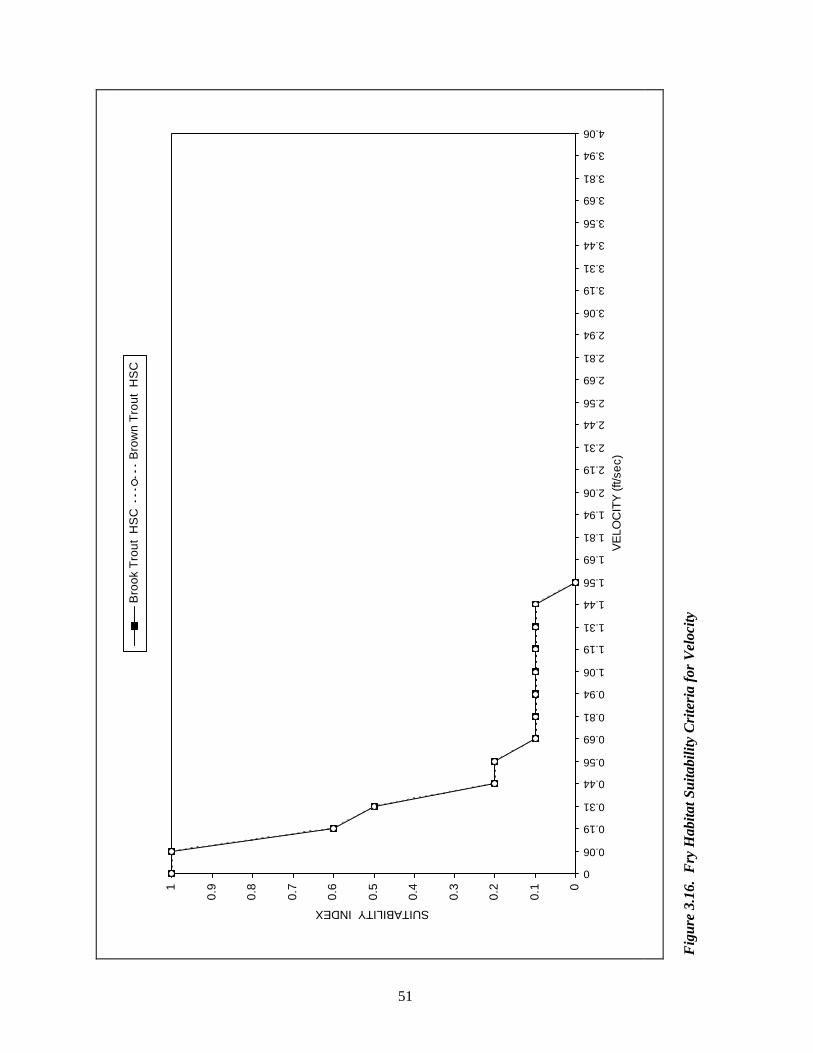
0

0.1

0.2

0.3

0.4

0.5

0.6

0.7

0.8

0.91

0

0.06

0.19

0.31

0.44

0.56

0.69

0.81

0.94

1.06

1.19

1.31

1.44

1.56

1.69

1.81

1.94

2.06

2.19

2.31

2.44

2.56

2.69

2.81

2.94

3.06

3.19

3.31

3.44

3.56

3.69

3.81

3.94

4.06

VE

LOC

ITY

(ft/s

ec)

SUITABILITY INDEXB

rook

Tro

ut H

SC

Bro

wn

Trou

t H

SC

Fig

ure

3.16

. F

ry H

abita

t Sui

tabi

lity

Cri

teri

a fo

r V

eloc

ity

51