Proactive Storage Health Management to Reduce Data Center Downtime(General Machine Learning)

Guanghua Shugshu@stanford.edu

Ji Eun Jangjiejang@stanford.edu

December 15, 2017

1 Abstract

The project adopts machine learning algorithms toperform proactive storage health management to re-duce data center down time. Specifically, we developreliable algorithms that can predict disk drive failuresfor timely replacement. The dataset is a collectionof SMART disk drive attributes provided by Back-Blaze. To construct compact time-series for modeldevelopment, three techniques are used to processSMART attribute data, including time-series aver-aging, feature selection, and class balancing. Modelsbased on four algorithms, including logistic regres-sion (LR), support vector machine (SVM), extremegradient boosting (XGBoost), and recurrent neuralnetwork (RNN), are developed and evaluated usingprediction accuracy and F-score along with precisionand recall. The baseline model LR achieved 87.2%prediction accuracy and a F-score of 0.87 with rel-ative low recall of 0.82 for failed disks. Both pre-diction accuracy and F-score are improved in SVM,XGBoost, and RNN. Specifically, XGBoost and RNNachieved 94.9% and 94.1%, respectively with F-scoresabove 94%. More importantly, recalls of failed disksare improved to above 93% to greatly reduce the riskof false negative prediction. Finally, proactive pre-diction capability is explored to provide replacementsuggestion in advance. RNN is able to keep predictionaccuracy above 70% with 9 days of proactive time.

2 Motivation

It is critical to keep data centers continuously on. Thecosts of data center downtime have increased from$5, 617/minute in 2010 to $8,851/minute in 2016 ac-cording to a study conducted on 63 data centers inthe U.S. [1]. IT equipment failure is the most costlyreason for data center downtime and storage compo-nents have the most frequent failing rate in current

IT environments. Therefore, accurate failure pre-diction and timely replacement can decrease down-time costs and improve system reliability [2]. Thedefense mechanisms such as RAID to improve disksavailability and reliability are not enough to preventthe failures to severely impact data center operations[2]. There exists monitoring systems such as SMART(self-monitoring, analysis, and reporting technology)to continuously report drive health status [3]. How-ever, SMART has a large number of attributes andtheir effects on disk failure are poorly defined. In thisproject, we explore both traditional machine learningalgorithms and deep learning methods to predict diskfailure based on time-series of historic disk status.

3 Related Work

Many of existing SMART-based monitoring systemsare simple and threshold-based normalization, whichshows weak prediction power with failed disk recallscore of merely above 50% [2, 4]. There exist statisti-cal approaches to improve prediction accuracy [5, 6].Murray et al. implemented Naive Bayesian classi-fier and Support Vector Machine, but achieved lessthan 60% detection rate [7]. More recently, Botezatuet al. showed very high accuracy using regularizedgreedy forest (RGF), random forest (RF), and sup-port vector machine (SVM) [2]. Our project adoptsand expands some of data preprocessing techniquesfrom [2], and applies different machine learning algo-rithms including XGBoost and RNN.

4 Processing SMART

4.1 What is SMART?

Self-monitoring, analysis, and reporting technology(SMART) is a monitoring system for hard disk drives(HDDs) and solid-state disk drives (SDDs). SMART

1

collects and reports on various attributes related todrive reliability. There exist SMART datasets col-lected and published by Backblaze [3]. Among Back-blaze datasets, we choose Seagate disk drive datasetfrom year 2013 to 2017 to develop and test the algo-rithms.

It is difficult to train models with raw SMARTdata set mainly due to three issues. First, time-series SMART data needs to be averaged to reducenoise from noisy measurement as well as disk recov-ery mechanisms [2]. Effective averaging window sizesfor each attributes can be different as each attributesare correlated to different types of failure mecha-nisms. Second, feature selection is necessary to de-cide which attributes are most indicative of impend-ing disk failure. SMART standard defines more than90 attributes. Moreover, each disk model has differ-ent dominant failure mechanisms, and hence differ-ent sets of effective attributes. Third, as disk driveshave a low failure rate, the data set is heavily class-imbalanced. Without proper class balacning, classifi-caion accuracy for the class with a small training size(i.e. failed disks) can be significantly degraded. Therest of this section addresses these three issues.

4.2 Window Averaging

An averaging window size is decided by change pointanalysis. Our change point analysis build a time se-ries model based on linear local trend model in (4.1),where yt is observation at time t, µt is a slowly vary-ing component called trend, νt is a slope term gener-ated by a random walk [8]. Three model parameters,σε, σξ, and σζ are estimated by maximizing its log-likelihood [9].

yt = µt + εt εt ∼ N (0, σ2ε )

µt+1 = µt + νt + ξt ξt ∼ N (0, σ2ξ )

νt+1 = νt + ζt ζt ∼ N (0, σ2ζ )

(4.1)

Assuming there exists a change point τ when ameaningful change occurs in attribute values, webuild two linear local trend models before and afterτ . Then, an optimal change point τmax is decidedto maximize sum of log-likelihood of two models. Ifparameters of two models before and after τmax aresignificantly different, the attribute is indicative ofdisk failure and the measured change point is valid.

τmax = argmaxτ

log(p(y1:τ−1|θ1)) + log(p(yτ :t|θ2))

(4.2)

Table 1: Change point analysis results

ID Mean of CPs ID Mean of CPs5 12 187 17

190 14 193 17194 17 197 17198 17 240 22241 20 242 15

Table 2: Accuracy with class balancing for linear SVM

Balancing technique AccuracyRandom sampling 91.5%K-means sampling 94.1%

Weighted SVM 89.0%

We use mean values of valid change points to ad-just an effective window size of an averaging function.Table 1 lists mean values of valid change points forsome attributes. Then, raw values of the attributesare averaged with exponentially decreasing weightsas Equation (4.3), where the parameter α controls itssmoothing effect. We relate the mean values of validchange points to α as Equation (4.3) [10].

st = α× yt + (1− α)× st−1 with α =2

τ + 1(4.3)

4.3 Feature Selection

To decide which attribute is most indicative, we mea-sured accuracies of support vector machine (SVM)when the model is trained with only one attribute.Seagate drive model ST4000DM000 in Backblazedataset provides 24 attributes. Fig. 1 shows test ac-curacy for each attribute. Among all 24 attributes,the attribute 193 (load cycle count) was most effec-tive showing 80% accuracy, followed by attribute 187,194, and so on.

To measure accuracy improvement by adding fea-tures, we added features in an order of higher accu-racy shown in Fig. 1. Fig. 2 plots test and trainingaccuracies over the number of features. The test ac-curacy improved as more features are added and sat-urated with more than 15 features. We didn’t observeoverfitting up to 24 attributes.

2

Figure 1: SVM test accuracy with only one attribute

Figure 2: SVM test accuracy with multiple attributes

4.4 Class Balancing

To address the imbalanced-class issue, we tried threetechniques: random sampling, K-means sampling,and weighted support vector machine. Random sam-pling blindly chooses the same number of healthydisks as the number of failed disks. K-means sam-pling divides the healthy disk data set to the samenumber of clusters as the failed disks and use clustercentroids as a representative healthy disk data set.Weighted support vector machine sets the ratio ofpenalties for different classes to the inverse ratio ofthe training class sizes [11].

Table 2 lists test accuracy with one of the threedownsampling technique. Among three techniques,K-means sampling gave the best accuracy of 94.1%.However, applying K-means clustering on a healthydisk data set with a large number of samples took asignificant computing time. Therefore, accuracy test-ing for the rest of the paper used random sampling.

5 Methods

Four algorithms are explored including logistic regres-sion (LR), support vector machine (SVM), extremegradient boosting (XGBoost), and recurrent neuralnetwork (RNN). A brief description of each algorithmis provided with the same settings for the dataset. Ingeneral, the disk failure detection is treated as a bi-

nary classification problem. The target labels cantake only two values y ∈ {−1,+1}. Each input sam-ple (x ∈ Rn) is assumed to be independently andidentically sampled from real world data distribution(iid) and m is the number of training samples.

5.1 Logistic Regression

The probabilistic view of LR is presented with thehelp of sigmoid function (g(z)) that converts the re-sults of hypothesis into probability model. With theiid assumption for samples and labels y ∈ {−1,+1},the log-likelihood can be derived as [12]

`(θ) =

m∑i=1

log p(Y = y(i)|x(i); θ)

= −m∑i=1

log(

1 + exp(−y(i)θTx(i)))

(5.1)

Where parameter θ ∈ Rn is to be learned duringtraining and yθTx is known as margin. Intuitively,when margins are positive (predictions are correctand y has the same sign as θTx), `(θ) approachesmaximum value 0. Conversely, negative margins re-sult in `(θ) stays more negative. The goal of LRalgorithm is to maximize the log-likelihood in Equa-tion (5.1). Finally, the LR algorithm has been imple-mented in Tensorflow [13] framework (LR from scikit-learn library[11] is used to confirm the correctnessof our own implementation and for cross-validation).Same as for other algorithms described later, mini-batch Gradient Descent is used to learn the parame-ter θ either by maximizing likelihood or minimizingloss. The learning rate and batch size are the twohyper-parameters been tuned in the process.

5.2 Support Vector Machines

The goal of support vector machine is to find a hy-perplane that separates the datasets with maximizedminimum margins (distances from support vectors tohyperplane). In SVM, hinge loss is generally usedin the loss function. Including the L2-regularization,the loss function for linear SVM becomes

J(W, b) =1

m

m∑i=1

[max(0, 1− y(i)(Wx(i) + b)] +λ

2‖W‖2

(5.2)

Both Linear SVM and SVM with Gaussian kernel(please refer to [12]) give similar performance in thisdataset. Fro simplicity, only the linear SVM perfor-mance is reported in the results session.

3

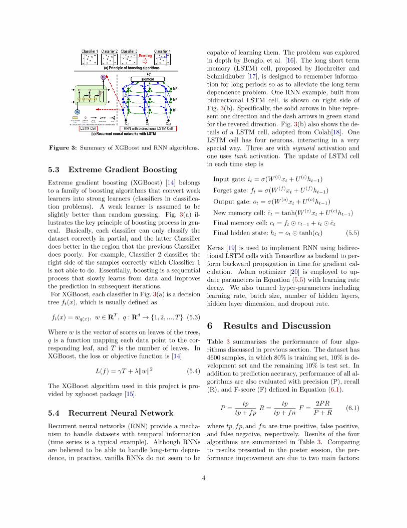
Figure 3: Summary of XGBoost and RNN algorithms.

5.3 Extreme Gradient Boosting

Extreme gradient boosting (XGBoost) [14] belongsto a family of boosting algorithms that convert weaklearners into strong learners (classifiers in classifica-tion problems). A weak learner is assumed to beslightly better than random guessing. Fig. 3(a) il-lustrates the key principle of boosting process in gen-eral. Basically, each classifier can only classify thedataset correctly in partial, and the latter Classifierdoes better in the region that the previous Classifierdoes poorly. For example, Classifier 2 classifies theright side of the samples correctly which Classifier 1is not able to do. Essentially, boosting is a sequentialprocess that slowly learns from data and improvesthe prediction in subsequent iterations.For XGBoost, each classifier in Fig. 3(a) is a decision

tree ft(x), which is usually defined as

ft(x) = wq(x), w ∈ RT , q : Rd → {1, 2, ..., T} (5.3)

Where w is the vector of scores on leaves of the trees,q is a function mapping each data point to the cor-responding leaf, and T is the number of leaves. InXGBoost, the loss or objective function is [14]

L(f) = γT + λ‖w‖2 (5.4)

The XGBoost algorithm used in this project is pro-vided by xgboost package [15].

5.4 Recurrent Neural Network

Recurrent neural networks (RNN) provide a mecha-nism to handle datasets with temporal information(time series is a typical example). Although RNNsare believed to be able to handle long-term depen-dence, in practice, vanilla RNNs do not seem to be

capable of learning them. The problem was exploredin depth by Bengio, et al. [16]. The long short termmemory (LSTM) cell, proposed by Hochreiter andSchmidhuber [17], is designed to remember informa-tion for long periods so as to alleviate the long-termdependence problem. One RNN example, built frombidirectional LSTM cell, is shown on right side ofFig. 3(b). Specifically, the solid arrows in blue repre-sent one direction and the dash arrows in green standfor the revered direction. Fig. 3(b) also shows the de-tails of a LSTM cell, adopted from Colah[18]. OneLSTM cell has four neurons, interacting in a veryspecial way. Three are with sigmoid activation andone uses tanh activation. The update of LSTM cellin each time step is

Input gate: it = σ(W (i)xt + U (i)ht−1)

Forget gate: ft = σ(W (f)xt + U (f)ht−1)

Output gate: ot = σ(W (o)xt + U (o)ht−1)

New memory cell: ct = tanh(W (c)xt + U (c)ht−1)

Final memory cell: ct = ft � ct−1 + it � ctFinal hidden state: ht = ot � tanh(ct) (5.5)

Keras [19] is used to implement RNN using bidirec-tional LSTM cells with Tensorflow as backend to per-form backward propagation in time for gradient cal-culation. Adam optimizer [20] is employed to up-date parameters in Equation (5.5) with learning ratedecay. We also tunned hyper-parameters includinglearning rate, batch size, number of hidden layers,hidden layer dimension, and dropout rate.

6 Results and Discussion

Table 3 summarizes the performance of four algo-rithms discussed in previous section. The dataset has4600 samples, in which 80% is training set, 10% is de-velopment set and the remaining 10% is test set. Inaddition to prediction accuracy, performance of all al-gorithms are also evaluated with precision (P), recall(R), and F-score (F) defined in Equation (6.1).

P =tp

tp+ fpR =

tp

tp+ fnF =

2PR

P +R(6.1)

where tp, fp, and fn are true positive, false positive,and false negative, respectively. Results of the fouralgorithms are summarized in Table 3. Comparingto results presented in the poster session, the per-formance improvement are due to two main factors:

4

Table 3: Algorithm performance summary

LR SVM XGBoost RNN

Accuracy [%]Train 90.6 91.5 99.9 97.2Test 87.2 88.7 94.9 94.1

FailedPrecision 0.92 0.96 0.96 0.95

Recall 0.82 0.89 0.93 0.93F-score 0.87 0.93 0.95 0.94

HealthyPrecision 0.83 0.90 0.93 0.94

Recall 0.93 0.93 0.97 0.95F-score 0.88 0.97 0.95 0.94

Figure 4: Error analysis for RNN model.

i) increase of dataset size (about 5x); and ii) accu-rate smoothing window for each feature (20 days wasapplied to all features in previous results).

6.1 Error Analysis

False negative error, predicting failed disk as healthyones, is most costly since undetected disk failures di-rectly lead to increase of data center down time. Thisis directly relate to recall of failed disks (also preci-sion of healthy disks) in Table 3. Although preci-sion and recall are fairly well balanced, there doesexist a uniform trend of lower recall in failed disksand lower precision in healthy ones which suggeststhat false negative error is one of the main errors.Here, we want to look into the false negative casesin RNN model to gain some understanding about thereason why the model makes such errors. Two obser-vations can be made on Fig. 4 showing true negative,false negative and true positive samples with 7 dif-ferent features. First, comparing false negative totrue negative samples, it is not surprising that falsenegative happens since most of the attributes are es-sentially the same. The only slight difference is thatsmart 1 in false negative case tends to have morenegative part and random fluctuation. Second, com-paring false negative to true positive vs, this tendsto suggest that in order for a sample to be classifiedas positive, in addition to the negativity and randomfluctuation in smart 1, other attributes should also

Figure 5: Proactive prediction accuracy.

have some kind of variations that related to failures.

6.2 Proactive Failure Prediction

Proactive prediction capability is also evaluated.With models only trained once on time series of com-plete disk life cycles, we test the accuracy of trainedmodels with test time series that have last n daysclose to the end of the disk life cycles been removed(proactive time). Such accuracy is defined as proac-tive prediction accuracy. The experiment results inFig. 5 show that proactive accuracy drops as proac-tive time increases for all algorithms, since the testsamples bear less similarity to the training set withincreasing proactive time. Note that the proactiveprediction accuracy in RNN decreases slower com-pared to other models as the proactive time increases,suggesting RNN has better proactive prediction ca-pability. This may be related to the inherent natureof RNN, designed to preserve long-term information.

7 Conclusion and Future Work

XGBoost achieved best prediction accuracy of 94.9%with RNN closely follows (94.1%) and F-scores andrecalls for failed disks are high for both. This sug-gests both XGBoost and RNN can fit time series andgeneralize well enough on test set with complete disklife cycles. However, RNN keeps proactive predic-tion accuracy above 70% with proactive time up to9 days, while the accuracy for XGBoost drops below70% beyond 5 days. This suggests RNN may gener-alize better with long-term dependence.Two future directions for this project: i) trans-fer learning between different disk models that haveslightly different attributes; ii) develop algorithm forbetter proactive prediction accuracy.

5

8 Contributions

Both group member have been actively contributingto the projects. A lot of study and discussion havebeen helpful to improve the project. We have beenworking interactively, with Ji Eun leading data pre-processing and Guanghua focusing on building algo-rithms and evaluating the performance.

References

[1] P. Institute, “Cost of data center outages,” 2016.[Online]. Available: https://www.ponemon.org/blog/2016-cost-of-data-center-outages

[2] M. M. Botezatu, I. Giurgiu, J. Bogojeska, andD. Wiesmann, “Predicting disk replacement to-wards reliable data centers,” in Proceedings ofthe 22Nd ACM SIGKDD International Confer-ence on Knowledge Discovery and Data Mining,2016, pp. 39–48.

[3] B. Beach, “Hard drive smart stats,” 2014.[Online]. Available: https://www.backblaze.com/blog/hard-drive-smart-stats/

[4] E. Pinheiro, W.-D. Weber, and L. A. Barroso,“Failure trends in a large disk drive population.”in FAST, vol. 7, no. 1, 2007, pp. 17–23.

[5] G. F. Hughes, J. F. Murray, K. Kreutz-Delgado,and C. Elkan, “Improved disk-drive failure warn-ings,” IEEE Transactions on Reliability, vol. 51,no. 3, pp. 350–357, 2002.

[6] B. Schroeder and G. A. Gibson, “Disk failuresin the real world: What does an mttf of 1, 000,000 hours mean to you?” in FAST, vol. 7, no. 1,2007, pp. 1–16.

[7] J. F. Murray, G. F. Hughes, and K. Kreutz-Delgado, “Machine learning methods for predict-ing failures in hard drives: A multiple-instanceapplication,” Journal of Machine Learning Re-search, vol. 6, no. May, pp. 783–816, 2005.

[8] J. Commandeur and S. Koopman, , An Introduc-tion to State Space Time Series Analysis. Ox-ford, 2007.

[9] J. Perktold, S. Seabold, and J. Taylor,“Statsmodels: statistics in python,” Oct. 2017.[Online]. Available: http://www.statsmodels.org/stable/index.html

[10] “Exponentially weighted windows,” Oct. 2017.[Online]. Available: http://pandas.pydata.org/pandas-docs/stable/computation.html#exponentially-weighted-windows

[11] F. Pedregosa, G. Varoquaux, A. Gramfort,V. Michel, B. Thirion, O. Grisel, M. Blondel,P. Prettenhofer, R. Weiss, V. Dubourg, J. Van-derplas, A. Passos, D. Cournapeau, M. Brucher,M. Perrot, and E. Duchesnay, “Scikit-learn: Ma-chine learning in Python,” Journal of MachineLearning Research, vol. 12, pp. 2825–2830, 2011.

[12] A. Ng, “Support vector machines,” Dec. 2017.[Online]. Available: cs229.stanford.edu/notes/cs229-notes2.pdf

[13] M. Abadi, A. Agarwal, P. Barham, E. Brevdo,Z. Chen, C. Citro, G. S. Corrado, A. Davis,J. Dean, M. Devin, S. Ghemawat, I. J.Goodfellow, A. Harp, G. Irving, M. Isard,Y. Jia, R. Jozefowicz, L. Kaiser, M. Kudlur,J. Levenberg, D. Mane, R. Monga, S. Moore,D. G. Murray, C. Olah, M. Schuster, J. Shlens,B. Steiner, I. Sutskever, K. Talwar, P. A.Tucker, V. Vanhoucke, V. Vasudevan, F. B.Viegas, O. Vinyals, P. Warden, M. Wat-tenberg, M. Wicke, Y. Yu, and X. Zheng,“Tensorflow: Large-scale machine learning onheterogeneous distributed systems,” CoRR,vol. abs/1603.04467, 2016. [Online]. Available:http://arxiv.org/abs/1603.04467

[14] T. Chen and C. Guestrin, “Xgboost: Ascalable tree boosting system,” CoRR, vol.abs/1603.02754, 2016. [Online]. Available: http://arxiv.org/abs/1603.02754

[15] D. D. M. L. Community, “Scalable, protableand distributed gradient boosting,” Aug. 2015.[Online]. Available: https://github.com/dmlc/xgboost

[16] Y. Bengio, P. Simard, and P. Frasconi, “Learn-ing long-term dependencies with gradient de-scent is difficult,” IEEE Transactions on NeuralNetworks, vol. 5, no. 2, pp. 157–166, Mar 1994.

[17] S. Hochreiter and J. Schmidhuber, “Lstm cansolve hard long time lag problems,” in Advancesin Neural Information Processing Systems 9.MIT Press, 1997, pp. 473–479.

6

[18] C. Colah, “Understanding lstm networks,” Aug.2015. [Online]. Available: http://colah.github.io/posts/2015-08-Understanding-LSTMs/

[19] F. Chollet et al., “Keras,” https://github.com/fchollet/keras, 2015.

[20] D. P. Kingma and J. Ba, “Adam: Amethod for stochastic optimization,” CoRR,vol. abs/1412.6980, 2014. [Online]. Available:http://arxiv.org/abs/1412.6980

7