31

3 Proton NMR on Cross-linked Polymers The type of molecular motion of a polymer sample is encoded in the shape of the transversal

relaxation (T2) curve. T2 is therefore sensitive to the physical environment of the probe

molecule. The most important application of this property is the determination of the mean

molecular mass between two cross-linked points (Mc). The theory behind the “decoding”

process and two practical methods for determination of the Mc values, together with the

corresponding results calculated for rubber samples (EPDM’s) are presented in this chapter.

Also, we demonstrate the impossibility to apply the same procedure for determining the cross-

link density of the rubber phase in a blended sample starting from proton T2.

32

3.1 Dipolar Residual Coupling and Proton NMR Relaxation 3.1.1 Introduction

The goal of the most studies is the establishment of the relationship among the molecular

structure, dynamics and physical properties of final materials. A useful application is connected

with the determination of the material cross-link density, which is responsible for important

mechanical features of elastomers. An important advantage of the NMR methods, in

comparison with the most conventional methods such as swelling and stress-strain

measurements is that NMR is a non-destructive technique. And more than that, as we will see

through the following chapters, in some cases, the NMR is the only technique that can be

applied in order to determine the material cross-link density.

During vulcanization process a certain amount of chemical cross-links are formed and, as a

consequence, the degree of freedom of the molecules is decreasing. The change of molecular

mobility can be well monitored indirectly by NMR relaxation. A lot of progress has been made

in the field of elastomer characterization using spin-spin (T2) NMR relaxation. Some well-

established NMR methods like Hahn-echo and its derivates, for example the “reduced WISE”30

(13C-edited proton transverse relaxation), the “sine correlation echo”, introduced by Callaghan

and Samulski31, and the stimulated echo used by Kimmich et.al.32, deliver valuable information

about the structure and the relaxation behavior of elastomers. Usually, for the interpretation of

the transversal NMR relaxation results are used two well-known models: Gotlib model33, 34 and

Sotta-Fülber model35. The main difference between the two models consists in the assumption

of a distribution either of the end-to-end distances of the polymeric chains (Sotta-Fülber) or of

the dipolar interaction under consideration (Gotlib-model).

In the present work we determined the cross-link density of EPDM using Gotlib-model and

Litvinov method36. The results are compared with swelling experiments data. We will also

explain and demonstrate why these methods are not suitable in the case of blends consisting in

polypropylene and EPDM.

33

3.1.2 The Transverse NMR Relaxation

While in liquid state the NMR relaxation times, i.e. spin-lattice relaxation (T1) and spin-spin

relaxation (T2), can be considered equal, in solid state they have different values. The study of

T1 and T2 can lead to valuable knowledge about molecular structure and motion and chemical

rate processes. This work is concerned with transversal relaxation (T2) and considers the

information related to the polymeric structure and dynamics.

In the present chapter we present the theoretical and experimental aspects of proton transverse

relaxation. The following treatment can be actually extended also to 13C transversal relaxation.

Protons are spin ½ nuclei and consequently, when placed in an external magnetic field, they

align independently of each other parallel or anti-parallel to the external field. The ratio of

parallel spins to the anti-parallel ones is given by the Boltzmann distribution

0exp( ) exp( )Bn En kT kT

γ+

−

∆= =

h (3.1)

Both energy levels are nearly equally populated, because the energy difference is very small in

comparison with thermic movements (kT). At T=300 K and a magnetic field of 18.7 T (800

MHz) the excess in the lower energy level is only 6.4 of 10000 particles for protons. This is the

main reason for the inherently low sensitivity of NMR when compared to optical spectroscopic

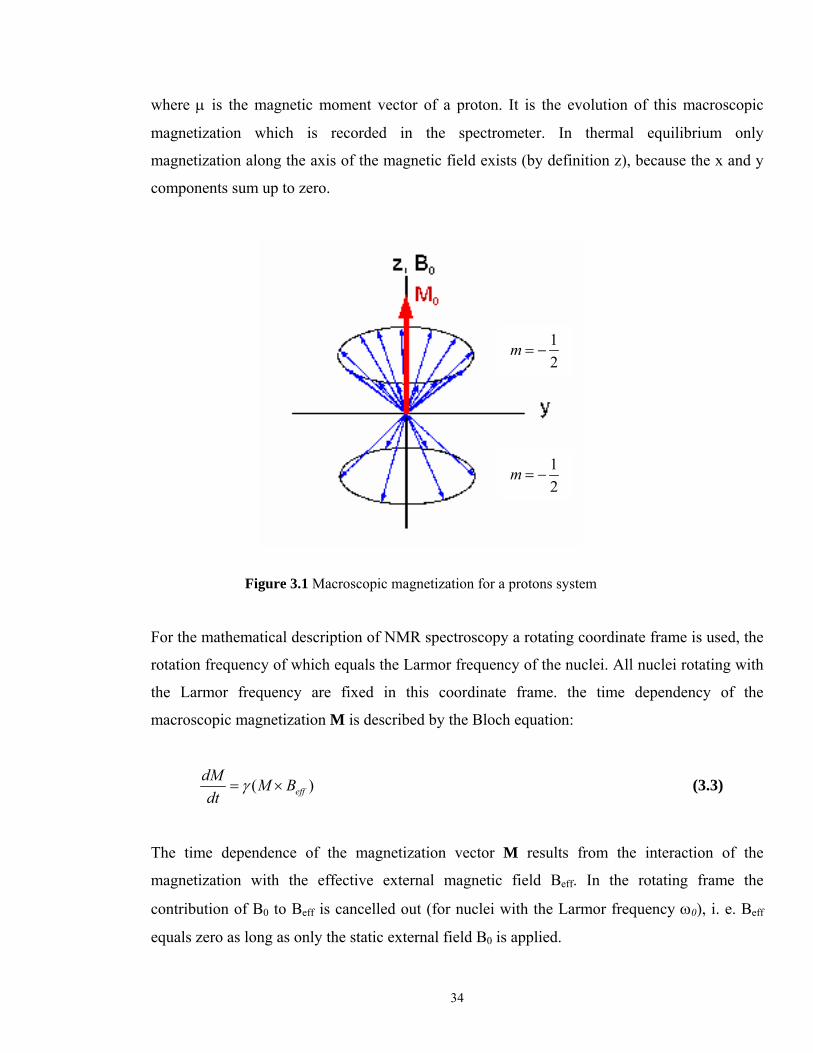
methods. However, we obtain a slight resultant magnetization in the positive z direction, see

Figure 3.1, after mathematically pairing the magnetic moments of the nuclei, up with down.

This magnetization is known as the bulk or macroscopic magnetization M and is defined as

follows

protons

M µ= ∑ (3.2)

34

where µ is the magnetic moment vector of a proton. It is the evolution of this macroscopic

magnetization which is recorded in the spectrometer. In thermal equilibrium only

magnetization along the axis of the magnetic field exists (by definition z), because the x and y

components sum up to zero.

Figure 3.1 Macroscopic magnetization for a protons system

For the mathematical description of NMR spectroscopy a rotating coordinate frame is used, the

rotation frequency of which equals the Larmor frequency of the nuclei. All nuclei rotating with

the Larmor frequency are fixed in this coordinate frame. the time dependency of the

macroscopic magnetization M is described by the Bloch equation:

( )effdM M Bdt

γ= × (3.3)

The time dependence of the magnetization vector M results from the interaction of the

magnetization with the effective external magnetic field Beff. In the rotating frame the

contribution of B0 to Beff is cancelled out (for nuclei with the Larmor frequency ω0), i. e. Beff

equals zero as long as only the static external field B0 is applied.

12

m = −

12

m = −

35

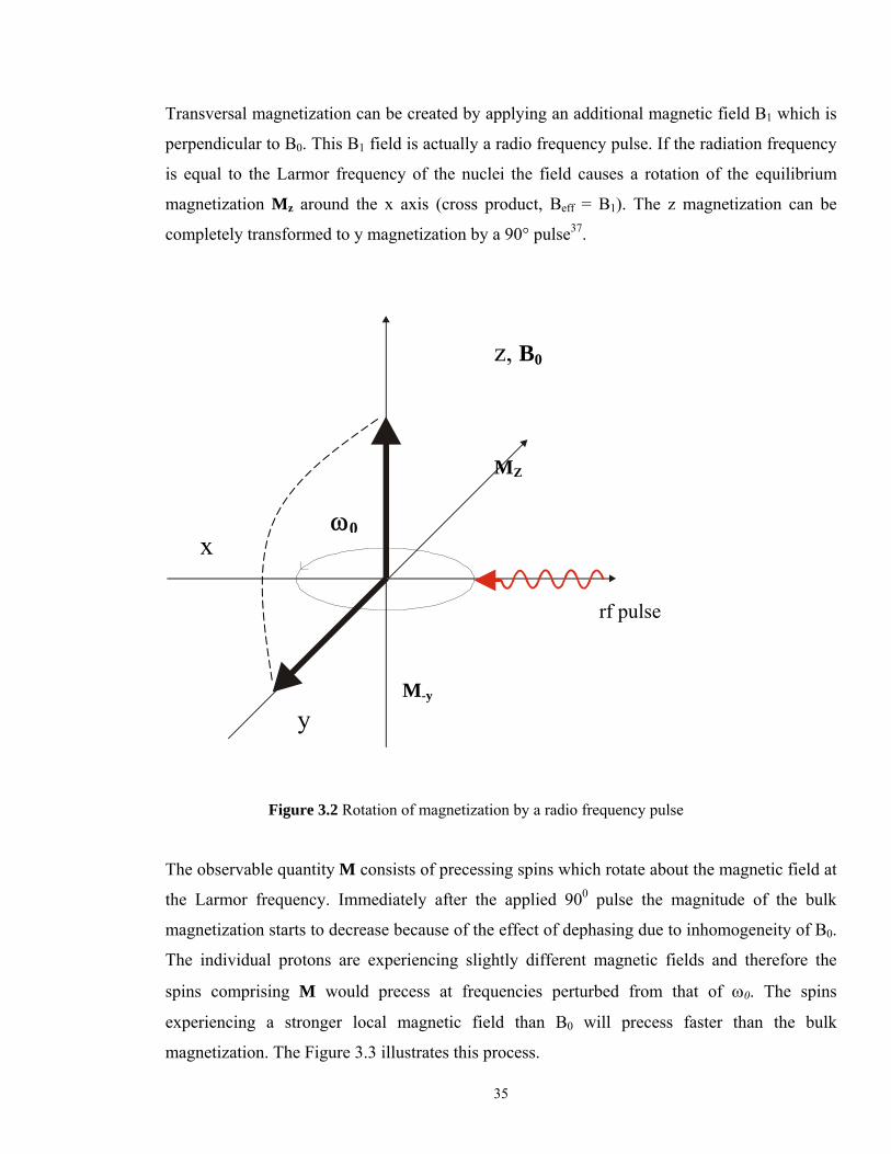
Transversal magnetization can be created by applying an additional magnetic field B1 which is

perpendicular to B0. This B1 field is actually a radio frequency pulse. If the radiation frequency

is equal to the Larmor frequency of the nuclei the field causes a rotation of the equilibrium

magnetization Mz around the x axis (cross product, Beff = B1). The z magnetization can be

completely transformed to y magnetization by a 90° pulse37.

Figure 3.2 Rotation of magnetization by a radio frequency pulse The observable quantity M consists of precessing spins which rotate about the magnetic field at

the Larmor frequency. Immediately after the applied 900 pulse the magnitude of the bulk

magnetization starts to decrease because of the effect of dephasing due to inhomogeneity of B0.

The individual protons are experiencing slightly different magnetic fields and therefore the

spins comprising M would precess at frequencies perturbed from that of ω0. The spins

experiencing a stronger local magnetic field than B0 will precess faster than the bulk

magnetization. The Figure 3.3 illustrates this process.

ω0

z, B0

rf pulse

y

x

MZ

M-y

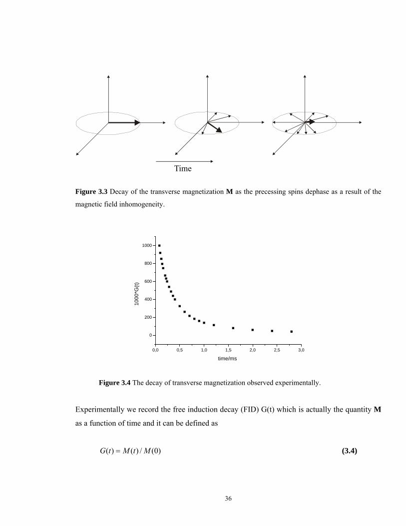
36

Time

Figure 3.3 Decay of the transverse magnetization M as the precessing spins dephase as a result of the

magnetic field inhomogeneity.

0,0 0,5 1,0 1,5 2,0 2,5 3,0

0

200

400

600

800

1000

1000

*G(t)

time/ms

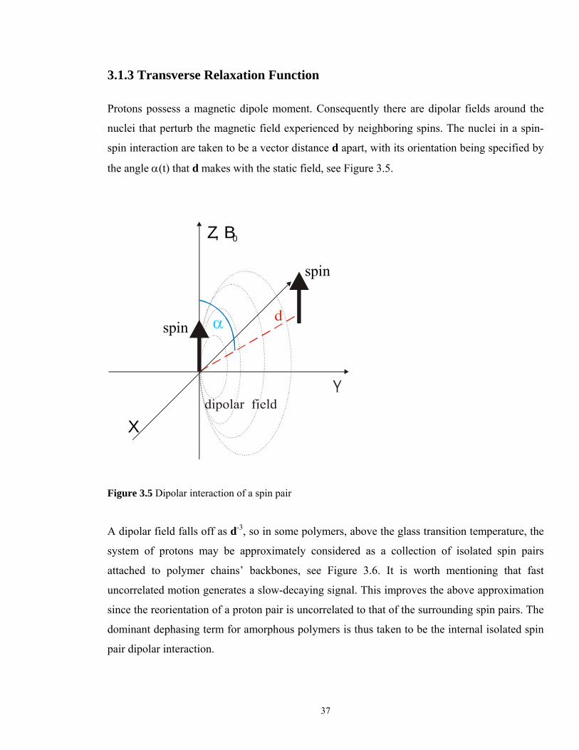
Figure 3.4 The decay of transverse magnetization observed experimentally.

Experimentally we record the free induction decay (FID) G(t) which is actually the quantity M

as a function of time and it can be defined as

)0(/)()( MtMtG = (3.4)

37

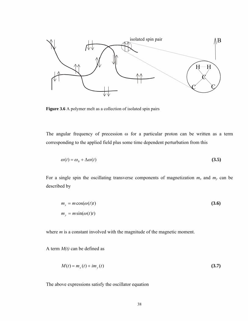
3.1.3 Transverse Relaxation Function

Protons possess a magnetic dipole moment. Consequently there are dipolar fields around the

nuclei that perturb the magnetic field experienced by neighboring spins. The nuclei in a spin-

spin interaction are taken to be a vector distance d apart, with its orientation being specified by

the angle α(t) that d makes with the static field, see Figure 3.5.

X

Z, B0

αspin

spin

Figure 3.5 Dipolar interaction of a spin pair

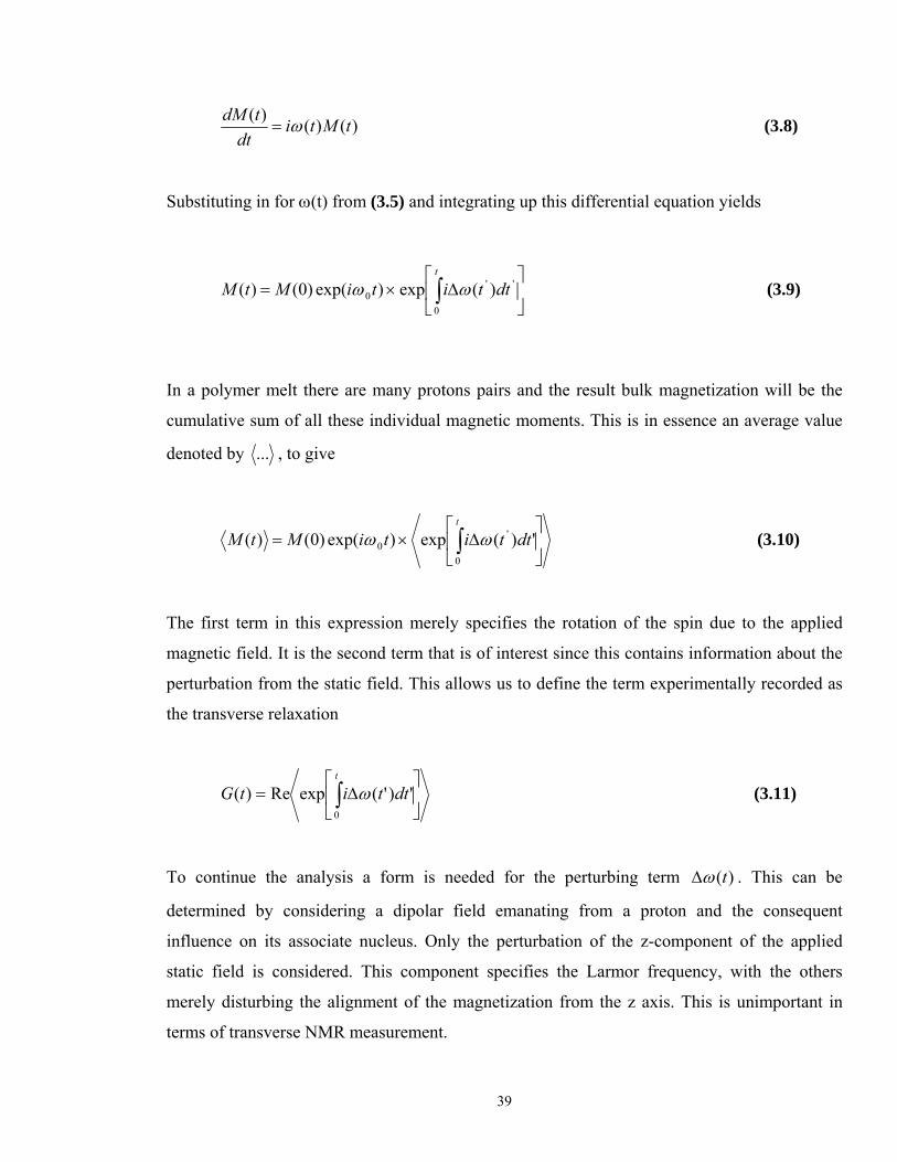
A dipolar field falls off as d-3, so in some polymers, above the glass transition temperature, the

system of protons may be approximately considered as a collection of isolated spin pairs

attached to polymer chains’ backbones, see Figure 3.6. It is worth mentioning that fast

uncorrelated motion generates a slow-decaying signal. This improves the above approximation

since the reorientation of a proton pair is uncorrelated to that of the surrounding spin pairs. The

dominant dephasing term for amorphous polymers is thus taken to be the internal isolated spin

pair dipolar interaction.

38

H H

CC C

isolated spin pair B

Figure 3.6 A polymer melt as a collection of isolated spin pairs

The angular frequency of precession ω for a particular proton can be written as a term

corresponding to the applied field plus some time dependent perturbation from this

)()( 0 tt ωωω ∆+= (3.5)

For a single spin the oscillating transverse components of magnetization mx and my can be

described by

))(cos( ttmmx ω= (3.6)

))(sin( ttmmy ω=

where m is a constant involved with the magnitude of the magnetic moment.

A term M(t) can be defined as

)()()( timtmtM yx += (3.7)

The above expressions satisfy the oscillator equation

39

)()()( tMtidt

tdM ω= (3.8)

Substituting in for ω(t) from (3.5) and integrating up this differential equation yields

⎥⎦

⎤⎢⎣

⎡∆×= ∫

t

dttitiMtM0

''0 )(exp)exp()0()( ωω (3.9)

In a polymer melt there are many protons pairs and the result bulk magnetization will be the

cumulative sum of all these individual magnetic moments. This is in essence an average value

denoted by ... , to give

⎥⎦

⎤⎢⎣

⎡∆×= ∫

t

dttitiMtM0

'0 ')(exp)exp()0()( ωω (3.10)

The first term in this expression merely specifies the rotation of the spin due to the applied

magnetic field. It is the second term that is of interest since this contains information about the

perturbation from the static field. This allows us to define the term experimentally recorded as

the transverse relaxation

⎥⎦

⎤⎢⎣

⎡∆= ∫

t

dttitG0

')'(expRe)( ω (3.11)

To continue the analysis a form is needed for the perturbing term )(tω∆ . This can be

determined by considering a dipolar field emanating from a proton and the consequent

influence on its associate nucleus. Only the perturbation of the z-component of the applied

static field is considered. This component specifies the Larmor frequency, with the others

merely disturbing the alignment of the magnetization from the z axis. This is unimportant in

terms of transverse NMR measurement.

40

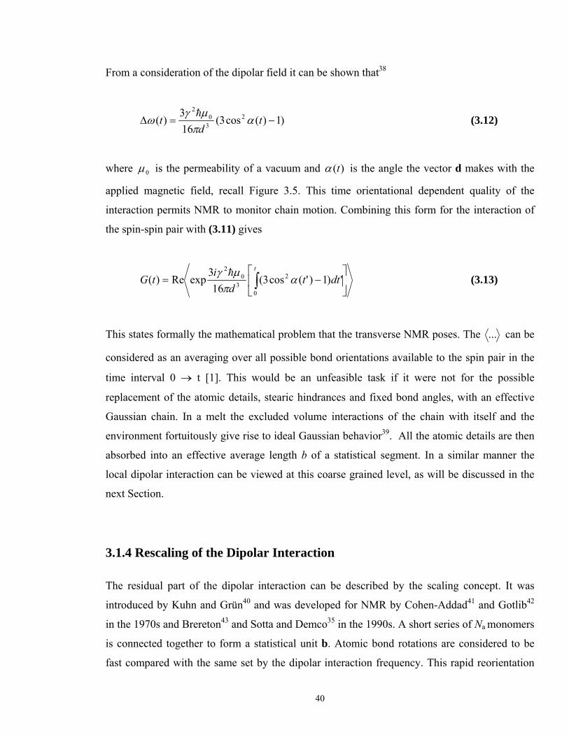
From a consideration of the dipolar field it can be shown that38

)1)(cos3(163

)( 230

2

−=∆ td

t απµγ

ωh

(3.12)

where 0µ is the permeability of a vacuum and )(tα is the angle the vector d makes with the

applied magnetic field, recall Figure 3.5. This time orientational dependent quality of the

interaction permits NMR to monitor chain motion. Combining this form for the interaction of

the spin-spin pair with (3.11) gives

⎥⎦

⎤⎢⎣

⎡−= ∫

t

dttd

itG

0

23

02

')1)'(cos3(16

3expRe)( α

πµγ h

(3.13)

This states formally the mathematical problem that the transverse NMR poses. The ... can be

considered as an averaging over all possible bond orientations available to the spin pair in the

time interval 0 → t [1]. This would be an unfeasible task if it were not for the possible

replacement of the atomic details, stearic hindrances and fixed bond angles, with an effective

Gaussian chain. In a melt the excluded volume interactions of the chain with itself and the

environment fortuitously give rise to ideal Gaussian behavior39. All the atomic details are then

absorbed into an effective average length b of a statistical segment. In a similar manner the

local dipolar interaction can be viewed at this coarse grained level, as will be discussed in the

next Section.

3.1.4 Rescaling of the Dipolar Interaction

The residual part of the dipolar interaction can be described by the scaling concept. It was

introduced by Kuhn and Grün40 and was developed for NMR by Cohen-Addad41 and Gotlib42

in the 1970s and Brereton43 and Sotta and Demco35 in the 1990s. A short series of Na monomers

is connected together to form a statistical unit b. Atomic bond rotations are considered to be

fast compared with the same set by the dipolar interaction frequency. This rapid reorientation

41

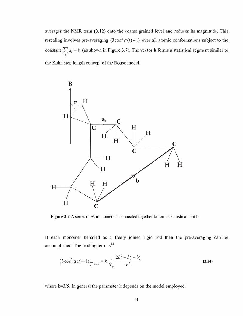
averages the NMR term (3.12) onto the coarse grained level and reduces its magnitude. This

rescaling involves pre-averaging )1)(cos3( 2 −tα over all atomic conformations subject to the

constant bai

i =∑ (as shown in Figure 3.7). The vector b forms a statistical segment similar to

the Kuhn step length concept of the Rouse model.

B

CC

CC

C

b

α

ai

Figure 3.7 A series of Na monomers is connected together to form a statistical unit b

If each monomer behaved as a freely joined rigid rod then the pre-averaging can be

accomplished. The leading term is44

2

2222 211)(cos3

bbbb

Nkt yxz

aba

ii

−−=

∑−

=α (3.14)

where k=3/5. In general the parameter k depends on the model employed.

42

The transverse relaxation (3.13) can now be rewritten using (3.14) as43

( ) ⎥⎦

⎤⎢⎣

⎡−−

∆= ∫

t

xyz dttbtbtbb

itG0

2222 ')'()'()'(2

23expRe)( (3.15)

where ∆ is the rescaled dipolar coupling constant

aNdk

30

2

8πµγ h

=∆ (3.16)

∆ is treated as an experimental parameter. For a proton pair with the distance apart

d measured in angstroms

134 )/(1059.1 −×=∆ sdNa

The description of the polymer molecule at a coarse grained level, by the chain vectors {b}, is

now assumed to obey Gaussian statistics. In this regime the Cartesian components are

independent and allows the problem to be further reduced to43

⎥⎦

⎤⎢⎣

⎡ ∆=∆ ∫

t

x dttbb

itg0

22 ')'(

23exp),( (3.17)

[ ]),(),(),2(Re)( tgtgtgtG ∆−∆−∆=

with the averaging now being taken over all possible conformations available to the sub-

molecule b in the time interval 0 → t.

The physics of the polymer melt, cross-links, entanglements and other chain interactions, is

introduced into the transverse decay through the averaging denoted by ... in (3.17). The type

of reorientation undergone by the probe molecule is indicative of its environment and can be

revealed through the shape of the transverse relaxation curve.

43

The problem (3.17) can be solved between two limits. Firstly fast dynamics where there is no

correlation between a bond vector at one time and a later moment. Secondly frozen dynamics

when the Gaussian bonds are essentially not re-orientating on the time scale of the NMR

experiment. These give two boundaries in which an NMR signal is expected to lie and indicates

the sensitivity of the decay curve to the NMR bond motion44.

The NMR signal varies from a simple single exponential to a complex algebraic decay as the

dynamics of the NMR molecule range from fast to slow. This gives a wide scope of possible

decays making NMR usefully sensitive to chain reorientation.

3.1.5 The Second Moments Approximation

The second moments approximation was proposed by Anderson and Weiss45 in 1953 and

Brereton46 discussed in 1991 its validity. Now it is possible to use this simplification within

certain known boundaries.

This method was an attempt to solve the problem (3.17) presented by the NMR experiment. It

made use of a well known statistics result for a random Gaussian variable X, which can be

stated as

( )⎥⎦⎤

⎢⎣⎡ −+= 22

21exp)exp( xXXX (3.31)

where ... indicates an average value found over a Gaussian distribution. In the transverse

relaxation problem (3.31) is compared with (3.17). From this likening the term X is given by

')'(23

0

22 dttb

biX

t

x∫∆

= (3.32)

The integral is replaced by a sum over discrete time and the dynamics are taken to be fast. Then

X becomes a summation of essentially independent random variables. This then produces the

required Gaussian statistics.

44

The term X is linear in ∆ and so will not survive the construction of G(t) from g(∆,t) see

(3.17). Applying (3.31) to the NMR problem and ignoring this linear term gives

( )⎥⎥⎦

⎤

⎢⎢⎣

⎡−⎟

⎠⎞

⎜⎝⎛ ∆−

=∆ ∫ ∫t t

xxxx dtdttbtbtbtbb

tg0 0

22222

2 "')"()'()"()'(23

21exp),( (3.33)

Since a Gaussian distribution is completely specified by its mean and variance the 4th order

correlation term presented above, )"()'( 22 tbtb xx , can usefully be rewritten from another

standard result

)"()'()"()'(2)"()'( 22222 tbtbtbtbtbtb xxxxxx +≡ (3.34)

to give

⎥⎥⎦

⎤

⎢⎢⎣

⎡⎟⎠⎞

⎜⎝⎛ ∆

−=∆ ∫ ∫t t

xx dtdttbtbb

tg0 0

22

2 "')"()'(23exp),( (3.35)

This result is the general starting point for a second moments approximation calculation. To

proceed a bond correlation function is needed and this can be that of single and multiple

relaxation times.

A bond relaxation function that bridges the two limits is that of a single exponential decay

⎟⎟⎠

⎞⎜⎜⎝

⎛ −=

1

2 "'exp

3)"()'(

τttbtbtb xx (3.36)

where τ1 is termed the correlation or relaxation time of the NMR active bond. It indicates the

rate of reorientation for the Gaussian link. A small τ1 implies rapid tumbling. A single

relaxation time is somewhat simplistic but it has the key features; at short times (t << τ1) the

bond appears frozen, and at long times (t >> τ1) the correlation tends to zero, i.e. the chain has

successfully completed many reorientations losing memory of its initial conformation.

45

The Rouse model (multiple relaxations) first appeared in 1953 in a paper by P. E. Rouse and is

a mechanical representation of the Gaussian chain47. The dynamics are governed by local

interactions along the chain and the physical constraint that a polymer cannot pass through

itself is ignored. It has been shown valid for low molecular weight polymer melts in rheological

experiments and more recently in NMR work48. The dynamics are then specified by a spectrum

of relaxation times49.

3.2 Different Methods of Crosslink Density Determination from Proton NMR Relaxation 3.2.1 Gotlib Model The Gotlib method for determining the mean molar mass between two cross-link points cM is

based, as in the case of other methods (i.e. Sotta, Litvinov and Brereton), on the fact that the

transverse NMR relaxation is sensitive to angular anisotropic segmental motion which is

spatially inhibited by chemical cross-links and topological hindrances. The persistence of

angular correlations on the time scale set by the residual dipolar interactions and the presence

of temporary or permanent constraints (entanglements or cross-links, respectively) leads to a

non-exponential decay of the transverse magnetization50. The shape of the line broadening

(“solid-like effect”) visualizes the dynamic influence of these constraints.

The residual part of the dipolar interaction is described by the scaling concept, the starting point

being the angular dependence of the dipolar interaction

)(cos)( 2 ααδω P⋅∆= (3.37)

where )8/( 3220 dhH πγµ=∆ is the coupling strength, h is the Planck constant, 0µ is the

magnetic moment and Hγ is the proton gyromagnetic ratio. )(cos2 αP represents the second

Legendre polynomial, and α is the angle between the interaction vector d, connecting the two

46

protons, and the static magnetic field B0. For an anisotropic rigid lattice of spin pairs the result

is 5/1)(cos 22 =αP , and the second moment 2

2 )(δω=rlM can be calculated as

222

22 20

9))(cos(49

∆=∆= αPM rl (3.38)

In the case of a very fast anisotropic motion (ν >>106 s-1) of the segment vector a in the

molecular system around the vector R the second moment can be reduced by pre-averaging to

the residual second moment M2Res of a slow and more isotropic motion (motional averaging).

Finally, the residual second moment of the dipolar interaction (general case) is given

2

2

22

2 51

49

⎟⎠⎞

⎜⎝⎛=⎟

⎠⎞

⎜⎝⎛∆=

nKM

nKM rlres (3.39)

where n is the number of statistical segments (Kuhn statistical segments) consisting in about 5

to 10 backbone bonds33 and K is a factor which depends on the geometry of the molecule.

The rapid anisotropic segmental motion of the network chains described by a number n of

freely rotating statistical segments leads to a nonzero average of the proton dipolar interaction

if the ends of this chain are fixed. The decay of the transverse proton NMR magnetization of

the network chain is described by

( )( ) ⎪⎭

⎪⎬⎫

⎪⎩

⎪⎨⎧

⎥⎦

⎤⎢⎣

⎡−+⎟⎟

⎠

⎞⎜⎜⎝

⎛−−−= 1expexp

02

22 ss

sres

N

N ttMTtA

MtM

τττ (3.40)

Here, A is the fraction of network chains in the system, T2 is the transversal relaxation time

related to the fast local motion and τs is the slow relaxation time for large scale rearrangements.

At this point is introduced42 a parameter to describe the anisotropy of the rapid motion. This is

defined as

47

2

2

2 ⎟⎠⎞

⎜⎝⎛==

nK

MMq rl

res

(3.41)

The factor K takes the value 3/5 in the case of a Gaussian chain and a direction of the dipolar

interaction vector parallel to the chain. In the case of a normal direction of the dipolar

interaction vector, like it is usually by C-H bonds of methylen or methyl groups, the factor K is

3/10 and 3/20, respectively.

The motion of free sol chains is assumed to be isotopic and yields to additionally purely

exponential decay37. Then, by assuming an anisotropic motion for the inter-cross-link chains

and the dangling free chain ends, the total NMR relaxation is described by 51, 34

( )( )

⎪⎭

⎪⎬⎫

⎪⎩

⎪⎨⎧−+

⎪⎭

⎪⎬⎫

⎪⎩

⎪⎨⎧

⎥⎦

⎤⎢⎣

⎡−+⎟⎟

⎠

⎞⎜⎜⎝

⎛−−−

+⎪⎭

⎪⎬⎫

⎪⎩

⎪⎨⎧

⎥⎦

⎤⎢⎣

⎡−+⎟⎟

⎠

⎞⎜⎜⎝

⎛−−−=

solsss

rl

sss

rl

N

N

TtCttMq

TtB

ttqMTtA

MtM

,22

'

2

22

2

exp1expexp

1expexp0

τττ

τττ

(3.42)

The fractions A, B and C represent the parts of magnetization of protons in inter-cross-link

chains, dangling ends and sol fraction, respectively. rlqM 2 represents the mean residual part of

the second moment of the dipolar interaction in relation to the physical and chemical

constrains. rlMq 2' is the same as before but much smaller and was introduced by Heuert et al.34

as a residual part of the second moment due to an assumed anisotropic motion of the dangling

chain ends.

The average molecular mass of inter-cross-link chains Sc nMM = can be determined. MS is the

molar mass of a statistical segment. Because of the influence of physical entanglements in real

networks, the value n that is obtained from equation (3.41) is not the true inter-cross-link

segmental number but an effective one. The influence of entanglements is taken into

consideration by correcting the value of q by a net value q0, which is obtained for the un-cross-

linked system. For the mean molar mass between two cross-links Mc it follows33, 52

48

sc Mqq

KM0−

= (3.43)

The experiments must be performed at a temperature well above glass transition temperature (T

= Tg + 120 K). Good correlation for many different rubbers was obtained between the Mc

values estimated from different methods for moderately cross-linked samples with Mc < 104

g/mol, while agreement between them was poor for loosely cross-linked samples with Mc > 104

g/mol50, 53. Parameters characterizing the network such as Mc, B, T2 and τs showed a similar

tendency as swelling and mechanical data50, 53, 54. The network parameters evaluated from the

different experimental techniques show fair agreement50.

3.2.2 Litvinov’s Method

Litvinov’s method for determining the mean molar mass of the network chains from proton

transversal relaxation in the vulcanized rubber is based also on Kuhn and Grün model of freely

joined chains. It is assumed that the network chain consists of Z statistical segments between

the network junctions42, 55. As in the case of other models, the T2 value is determined at a

temperature well above glass transition temperature, where a plateau region is detected.

For a Gaussian chain, in which the average, squared distance between network junctions is

much shorter than the contour chain length, the pT2 (transversal relaxation from the plateau

region) value is related to Z

rl

p

aTTZ

2

2= (3.44)

where a is the theory coefficient, which depends on the angle between the segment axis and the

internuclear vector for the nearest nuclear spins at the main chain. For polymers containing

aliphatic protons in the main chain, the coefficient a is close to 6.2 ± 0.755. The rlT2 value,

which is measured for swollen samples below glass transition temperature, is related to the

49

strength of intrachain proton-proton interaction in the rigid lattice56. The rlT2 value for a C2Cl4

swollen EPDM sample equals 10.4 ± 0.2 µs at 140 K57.

Using the number of backbone bonds in the statistical segment, ∞C , the molar mass of network

chain, wM is calculated

nMZCM uw /∞= (3.45)

where uM is the average molar mass per elementary chain unit for the copolymer chain and n

is the number of backbone bonds in an elementary chain unit. For the calculation of wM in the

case of EPDM the value of ∞C at 363 K is 6.62 and is considered for an alternating ethylene-

propylene copolymer58. It is assumed that the relative contribution of a network chain to the

total relaxation function for heterogeneous networks is proportional to the number of protons

attached to this chain. The cross-link density is defined by the value wfM/2 , where f is the

functionality of network junctions by which this chain is fixed.

The maximum, relative error of network density determination by Litvinov’s method is

estimated to be about 15-25%. This error is composed of absolute errors in the pT2 and rlT2 values and the inaccuracy of the coefficients a and ∞C 57.

3.3 Experimental detection of transverse NMR relaxation

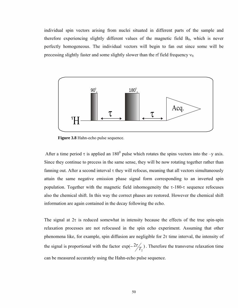
The spin echo phenomenon was accidentally discovered and named by Hahn59. The

corresponding pulse sequence (see Figure 3.8) measure the spin-spin relaxation time (T2) and

represents the most useful building block for eliminating B0 inhomogeneities.

At time zero a 900 pulse is applied along the positive x axis of the rotating frame, causing the

magnetization M to precess into the positive y axis. The magnetization is the vector sum of

50

individual spin vectors arising from nuclei situated in different parts of the sample and

therefore experiencing slightly different values of the magnetic field B0, which is never

perfectly homogeneous. The individual vectors will begin to fan out since some will be

precessing slightly faster and some slightly slower than the rf field frequency ν0.

HAcq.

900x 1800

y

τ τ

Figure 3.8 Hahn-echo pulse sequence.

After a time period τ is applied an 1800 pulse which rotates the spins vectors into the –y axis.

Since they continue to precess in the same sense, they will be now rotating together rather than

fanning out. After a second interval τ they will refocus, meaning that all vectors simultaneously

attain the same negative emission phase signal form corresponding to an inverted spin

population. Together with the magnetic field inhomogeneity the τ-180-τ sequence refocuses

also the chemical shift. In this way the correct phases are restored. However the chemical shift

information are again contained in the decay following the echo.

The signal at 2τ is reduced somewhat in intensity because the effects of the true spin-spin

relaxation processes are not refocused in the spin echo experiment. Assuming that other

phenomena like, for example, spin diffusion are negligible for 2τ time interval, the intensity of

the signal is proportional with the factor )2exp(2T

τ− . Therefore the transverse relaxation time

can be measured accurately using the Hahn-echo pulse sequence.

51

The phase cycling of the 1800 pulse in a spin echo experiment is called exorcycle. If the phase

of the 1800 pulse is varied through the sequence {x, y, -x, -y}, the magnetization refocuses

along the {y, -y, y, -y}. If the four signals are simply co-added, they would cancelled each

other, but if the receiver phase is adjusted in order to follow the refocused magnetization {y, -y,

y, -y} the signal will add up. In spectrometer encoding, the phase cycle would be written as:

• 0 1 2 3 (for the 1800 pulse)

• 0 2 0 2 (for the receiver).

For the present work all proton transversal relaxation time were carried out on a Varian

INOVA widebore spectrometer operating at 400 MHz for protons. The applied repetition time

of 3-4 s was longer than 5 T1, where T1 is the NMR spin-lattice relaxation time. Usually, 40

values of I(2τ) were measured in the time interval 2τ from 80µs to 120 ms, where I(2τ) is the

amplitude of an echo signal after the second pulse in the pulse sequence. The temperature for

all experiments was set to 80 0C.

3.4 Results and Discussions

3.4.1 Determination of the Network Density for EPDM Samples

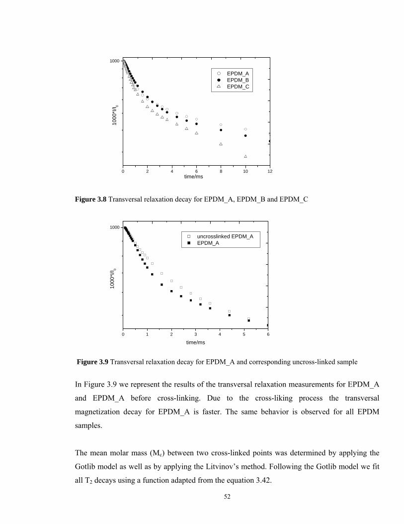
In order to determine the mean molar mass between two cross-linked points for the EPDM

samples, the proton transversal relaxation decay was recorded for each cross-linked sample as

well as for the corresponding uncross-linked EPDM. As expected, the EPDM_C shows the

fastest decay, indicating the highest amount of cross-links.

52

0 2 4 6 8 10 12

1000

1000

*I/I 0

time/ms

EPDM_A EPDM_B EPDM_C

Figure 3.8 Transversal relaxation decay for EPDM_A, EPDM_B and EPDM_C

0 1 2 3 4 5 6

1000

1000

*I/I 0

time/ms

uncrosslinked EPDM_A EPDM_A

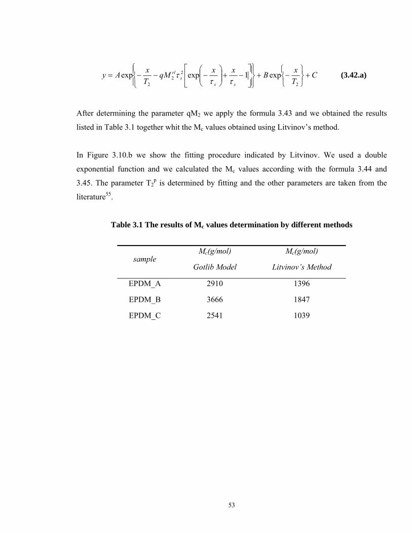
Figure 3.9 Transversal relaxation decay for EPDM_A and corresponding uncross-linked sample

In Figure 3.9 we represent the results of the transversal relaxation measurements for EPDM_A

and EPDM_A before cross-linking. Due to the cross-liking process the transversal

magnetization decay for EPDM_A is faster. The same behavior is observed for all EPDM

samples.

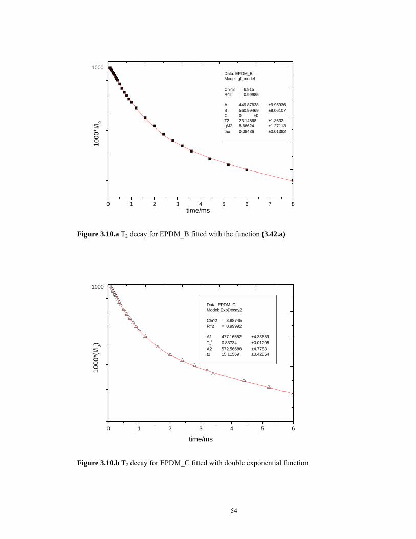
The mean molar mass (Mc) between two cross-linked points was determined by applying the

Gotlib model as well as by applying the Litvinov’s method. Following the Gotlib model we fit

all T2 decays using a function adapted from the equation 3.42.

53

CTxBxxqM

TxAy

sss

rl +⎭⎬⎫

⎩⎨⎧−+

⎪⎭

⎪⎬⎫

⎪⎩

⎪⎨⎧

⎥⎦

⎤⎢⎣

⎡−+⎟⎟

⎠

⎞⎜⎜⎝

⎛−−−=

2

22

2

exp1expexpττ

τ (3.42.a)

After determining the parameter qM2 we apply the formula 3.43 and we obtained the results

listed in Table 3.1 together whit the Mc values obtained using Litvinov’s method.

In Figure 3.10.b we show the fitting procedure indicated by Litvinov. We used a double

exponential function and we calculated the Mc values according with the formula 3.44 and

3.45. The parameter T2p is determined by fitting and the other parameters are taken from the

literature55.

Table 3.1 The results of Mc values determination by different methods

sample Mc(g/mol)

Gotlib Model

Mc(g/mol)

Litvinov’s Method

EPDM_A 2910 1396

EPDM_B 3666 1847

EPDM_C 2541 1039

54

0 1 2 3 4 5 6 7 8

1000Data: EPDM_BModel: gf_model Chi^2 = 6.915R^2 = 0.99985 A 449.87638 ±9.95936B 560.99469 ±9.06107C 0 ±0T2 23.14868 ±1.3632qM2 8.66624 ±1.27113tau 0.08436 ±0.01382

1000

*I/I 0

time/ms

Figure 3.10.a T2 decay for EPDM_B fitted with the function (3.42.a)

0 1 2 3 4 5 6

1000

Data: EPDM_CModel: ExpDecay2 Chi^2 = 3.88745R^2 = 0.99992 A1 477.16552 ±4.33659T2

p 0.83734 ±0.01205A2 572.56688 ±4.7783t2 15.11569 ±0.42854

1000

*(I/I

0)

time/ms

Figure 3.10.b T2 decay for EPDM_C fitted with double exponential function

55

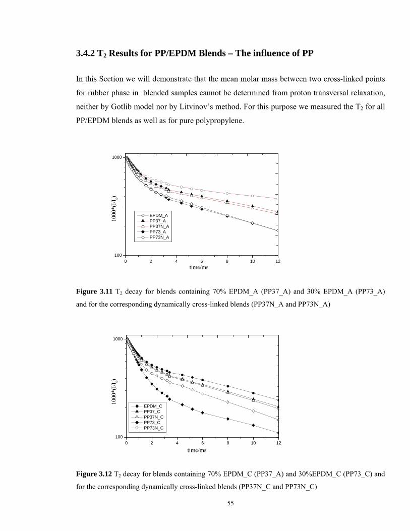
3.4.2 T2 Results for PP/EPDM Blends – The influence of PP

In this Section we will demonstrate that the mean molar mass between two cross-linked points

for rubber phase in blended samples cannot be determined from proton transversal relaxation,

neither by Gotlib model nor by Litvinov’s method. For this purpose we measured the T2 for all

PP/EPDM blends as well as for pure polypropylene.

0 2 4 6 8 10 12100

1000

EPDM_A PP37_A PP37N_A PP73_A PP73N_A

1000

*(I/I

0)

time/ms

Figure 3.11 T2 decay for blends containing 70% EPDM_A (PP37_A) and 30% EPDM_A (PP73_A)

and for the corresponding dynamically cross-linked blends (PP37N_A and PP73N_A)

0 2 4 6 8 10 12100

1000

EPDM_C PP37_C PP37N_C PP73_C PP73N_C

1000

*(I/I

0)

time/ms

Figure 3.12 T2 decay for blends containing 70% EPDM_C (PP37_A) and 30%EPDM_C (PP73_C) and

for the corresponding dynamically cross-linked blends (PP37N_C and PP73N_C)

56

Figures 3.11 and 3.12 show the proton transversal relaxation of different blends, including

dynamically cross-linked samples. The T2 decay is faster with the increase of polypropylene

content. The additionally cross-linked blend, PPN73_C, present a higher mobility (slower T2

decay) than the corresponding blend (PP73_C) obtained only by mechanically mixing the

rubber with polypropylene. This behaviour is due to the influence of the cross-linking agents

(Struktol) on polypropylene matrix.

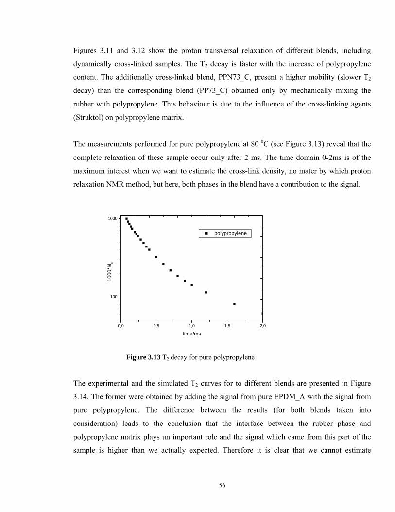
The measurements performed for pure polypropylene at 80 0C (see Figure 3.13) reveal that the

complete relaxation of these sample occur only after 2 ms. The time domain 0-2ms is of the

maximum interest when we want to estimate the cross-link density, no mater by which proton

relaxation NMR method, but here, both phases in the blend have a contribution to the signal.

0,0 0,5 1,0 1,5 2,0

100

1000

1000

*I/I 0

time/ms

polypropylene

Figure 3.13 T2 decay for pure polypropylene

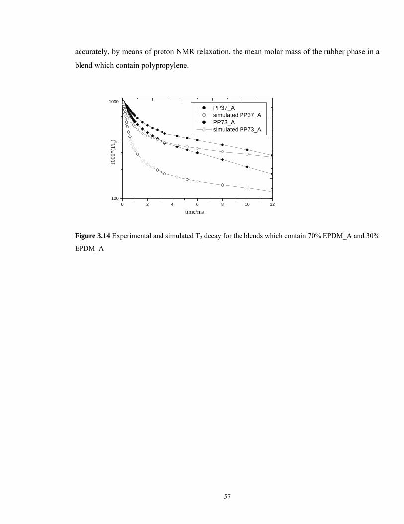
The experimental and the simulated T2 curves for to different blends are presented in Figure

3.14. The former were obtained by adding the signal from pure EPDM_A with the signal from

pure polypropylene. The difference between the results (for both blends taken into

consideration) leads to the conclusion that the interface between the rubber phase and

polypropylene matrix plays un important role and the signal which came from this part of the

sample is higher than we actually expected. Therefore it is clear that we cannot estimate

57

accurately, by means of proton NMR relaxation, the mean molar mass of the rubber phase in a

blend which contain polypropylene.

0 2 4 6 8 10 12100

1000 PP37_A simulated PP37_A PP73_A simulated PP73_A

1000

*(I/I

0)

time/ms

Figure 3.14 Experimental and simulated T2 decay for the blends which contain 70% EPDM_A and 30%

EPDM_A