Embed Size (px)
Citation preview

1
JAN. 30, 09 1
UP-SCALING OF SEBAL DERIVED 2
EVAPOTRANSPIRATION MAPS FROM LANDSAT (30m) 3
TO MODIS (250m) SCALE 4
5
Sung-ho Hong, Jan M.H. Hendrickx and Brian Borchers 6
New Mexico Tech, Socorro, NM 87801 7
8
9
ABSTRACT 10
11
Remotely sensed imagery of the Earth’s surface via satellite sensors provides information 12
to estimate the spatial distribution of evapotranspiration (ET). The spatial resolution of 13
ET predictions depends on the sensor type and varies from the 30 – 60 m Landsat scale to 14
the 250 – 1000 m MODIS scale. Therefore, for an accurate characterization of the 15
regional distribution of ET, scaling transfer between images of different resolutions is 16
important. Scaling transfer includes both up-scaling (aggregation) and down-scaling 17
(disaggregation). In this paper, we address the up-scaling problem. 18
19
The Surface Energy Balance Algorithm for Land (SEBAL) was used to derive ET maps 20
from Landsat 7 Enhanced Thematic Mapper Plus (ETM+) and Moderate Resolution 21
Imaging Spectroradiometer (MODIS) images. Landsat 7 bands have spatial resolutions of 22

2
30 to 60 m, while MODIS bands have resolutions of 250, 500 and 1000 m. Evaluations 23
were conducted for both “output” and “input” up-scaling procedures, with aggregation 24
accomplished by both simple averaging and nearest neighboring resampling techniques. 25
Output up-scaling consisted of first applying SEBAL and then aggregating the output 26
variable (daily ET). Input up-scaling consisted of aggregating 30 m Landsat pixels of the 27
input variable (radiance) to obtain pixels at 60, 120, 250, 500 and 1000 m before SEBAL 28
was applied. The objectives of this study were first to test the consistency of SEBAL 29
algorithm for Landsat and MODIS satellite images and second to investigate the effect of 30
the four different up-scaling processes on the spatial distribution of ET. 31
32
We conclude that good agreement exists between SEBAL estimated ET maps directly 33
derived from Landsat 7 and MODIS images. Among the four up-scaling methods 34
compared, the output simple averaging method produced aggregated data and aggregated 35
differences with the most statistically and spatially predictable behavior. The input 36
nearest neighbor method was the least predictable but was still acceptable. Overall, the 37
daily ET maps over the Middle Rio Grande Basin aggregated from Landsat images were 38
in good agreement with ET maps directly derived from MODIS images. 39
40
41
1. INTRODUCTION 42
43
Remote sensing data from satellite-based sensors have the potential to provide detailed 44
information on land surface properties and parameters at local to regional scales. Perhaps 45

3
one of the most important land surface parameters that can be derived from remote 46
sensing is actual ET. The spatio-temporal distribution of ET is needed for sustainable 47
management of water resources as well as for a better understanding of water exchange 48
processes between the land surface and the atmosphere. However, ground measurements 49
of ET over a range of space and time scales are very difficult to obtain due to the time 50
and cost involved. Remotely sensed imagery with numerous spatial and temporal 51
resolutions is therefore an ideal solution for determination of the spatio-temporal 52
distribution of ET. 53
54
Today, large amounts of remotely sensed data with variable spatial, temporal, and 55
spectral resolutions are available. A number of studies have attempted to estimate ET 56
from different satellite sensors, including the Land remote sensing satellite Enhanced 57
Thematic Mapper Plus (Landsat ETM+) (Bastiaanssen et al., 2005; Hendrickx and Hong, 58
2005; Allen et al., 2007; Hong, 2008), the Advanced Spaceborne Thermal Emission and 59
Reflection Radiometer (ASTER) (French et al., 2002), the Advanced Very High 60
Resolution Radiometer (AVHRR) (Seguin et al., 1991), the Moderate Resolution 61
Imaging Spectroradiometer (MODIS) (Nishida et al., 2003; Hong et al., 2005) and the 62
Geostationary Orbiting Environmental Satellite (GOES) (Mecikalski et al., 1999). 63
64
We employ the Surface Energy Balance Algorithm for Land (SEBAL) that is one of 65
several remote sensing algorithms used to extract information from raw satellite data. It 66
estimates various land surface parameters, including surface albedo, normalized 67
difference vegetation index (NDVI), surface temperature, and energy balance parameters 68

4
from the remotely sensed radiance values obtained from satellite sensors. Since satellite 69
sensors have different spatial, spectral and radiometric resolutions, the consistency of ET 70
estimates from different satellites by SEBAL needs to be certified. 71
72
The validation of products of remote sensing algorithms is dependent upon the spatial 73
resolution (Liang, 2004). Fine resolution products (< 100 m) such as Landsat can be 74
validated with ground measurements. However, validating coarse resolution products, 75
such as MODIS (1000 m in thermal band), using ground measurements is very difficult 76
because of the scale disparity between ground “point” measurements and the coarse 77
spatial resolution imagery. Therefore, for validation of MODIS products, the products of 78
high resolution remotely sensed imagery such as Landsat 7 (30 to 60 m resolution) need 79
to be first validated with ground point measurements. MODIS products can then be 80
compared against up-scaled (aggregated) Landsat product. A comparison of SEBAL ET 81
estimates against independent ground based measurements typically yields accuracies of 82
about 15% and 5% for, daily and seasonal evaporation estimates, respectively 83
(Bastiaanssen et al., 2005). In the southwestern USA, daily SEBAL ET estimates agreed 84
with ground observation with an accuracy of 10% (Hendrickx and Hong, 2005; Hong, 85
2008). Similar results have been reported by Morse et al. (2000) and Allen et al. (2007). 86
87
Many studies regarding the effect of up-scaling data sets have been reported (Mark and 88
Aronson, 1984; Nellis and Briggs, 1989; Turner et al., 1989; Lam and Quattrochi, 1992; 89
Stoms, 1992; Brown et al., 1993; Vieux, 1993; De Cola, 1994; Wolock and Price, 1994; 90
Zhang and Montgomery, 1994; Bian et al., 1999). During an aggregation process, the 91

5
raster spatial data are reduced to a smaller number of data pixels covering the same 92
spatial extent. It is generally recognized that data aggregation modifies the statistical and 93
spatial characteristics of the data (Bian et al., 1999). Since the total number of pixels is 94
reduced, the variance and frequency distribution of the sampled data may deviate from 95
the original data set and tends to reduce spatial autocorrelation at coarser resolutions 96
(Bian, 1997). Some studies have pointed out that data accuracy is enhanced significantly 97
by reduction of spatial resolution (Townshend et al., 1992; Dai and Khorram, 1998; Van 98
Rompaey et al., 1999; Carmel, 2004). Several studies have also argued that aggregation 99
to a coarser resolution reveals certain spatial patterns which are not shown until the data 100
are presented at a coarser scale (Zhang and Montgomery, 1994; Seyfried and Wilcox, 101
1995). On the other hand, the decrease in spatial resolution possibly results in a loss of 102
information that may be valuable for particular applications (Carmel et al., 2001). 103
104
The methodology for aggregating simple rectangular grid data is well developed (Bian, 105
1997; Bian et al., 1999; Mengelkamp et al., 2006). In this study, the simple averaging and 106
nearest neighbor resampling methods were selected for the data aggregation scheme, 107
since these methods have been the most popular and convenient to use (Atkinson, 1985; 108
Liang, 2004). The simple averaging method calculates the average value over an area of 109
interest to produce a new coarser resolution data set. Nearest neighbor sampling produces 110
a subset of the original data; the extremes and subtleties of the data values are therefore 111
preserved. 112
113

6
For the up-scaling scheme, numerous studies have used the assumption that surface 114
fluxes can be expressed as direct area averages of the surface fluxes (Shuttleworth, 1991; 115
Lhomme, 1992; Li and Avissar, 1994). Liang (2000) simply averaged the remotely 116
sensed reflectance values from 30 m to 1 km and explored the aggregation effect. He 117
concluded that the spectral reflectance was basically linear from 30 m resolution to 1000 118
m resolution. More recently, Mengelkamp et al (2006) mentioned that area averaged 119
small scale ET calculated from local measurements was in good agreement with the area 120
represented regional values. Nevertheless, few papers have examined the effect of 121
different up-scaling schemes on the relative accuracy of the aggregated data despite its 122
practical importance. A spatial resolution gap exists between the data requirements of 123
regional-scale models and the output data from remote sensing energy balance algorithms 124
such as SEBAL. For example, general global circulation models or regional weather 125
prediction models need input data with a spatial resolution of hundreds of kilometers 126
which is much larger than the spatial resolution of most satellite sensors (Liang, 2004). 127
Therefore, an up-scaling (data aggregation) procedure is needed to fill the scale gap 128
between satellite measurements and input requirements for large scale models. Increasing 129
spatial resolution by data aggregation has shown the potential to generate observed or 130
modeled surface flux estimates over a range of different spatial resolutions (Gupta et al., 131
1986; Lhomme, 1992; Ebleringer and Field, 1993). 132
133
In this study, high quality scenes of two different dates of Landsat 7 Enhanced Thematic 134
Mapper Plus (ETM+) and Moderate Resolution Imaging Spectroradiometer (MODIS) 135
imagery were selected and SEBAL was applied to estimate daily ET. Landsat scale pixels 136

7
(30 m) were aggregated to larger scale (60, 120, 250, 500 and 1000 m). The objectives of 137
this study were first to test the consistency of the SEBAL algorithm for Landsat 7 and 138
MODIS images, and second to investigate the effects of four different up-scaling 139
processes on the spatial distribution of ET, especially how the relative accuracy of ET 140
changes with different up-scaling processes. 141
142
143
2. METHOD AND MATERIALS 144
145
2.1. STUDY AREA AND SATELLITE IMAGERY 146
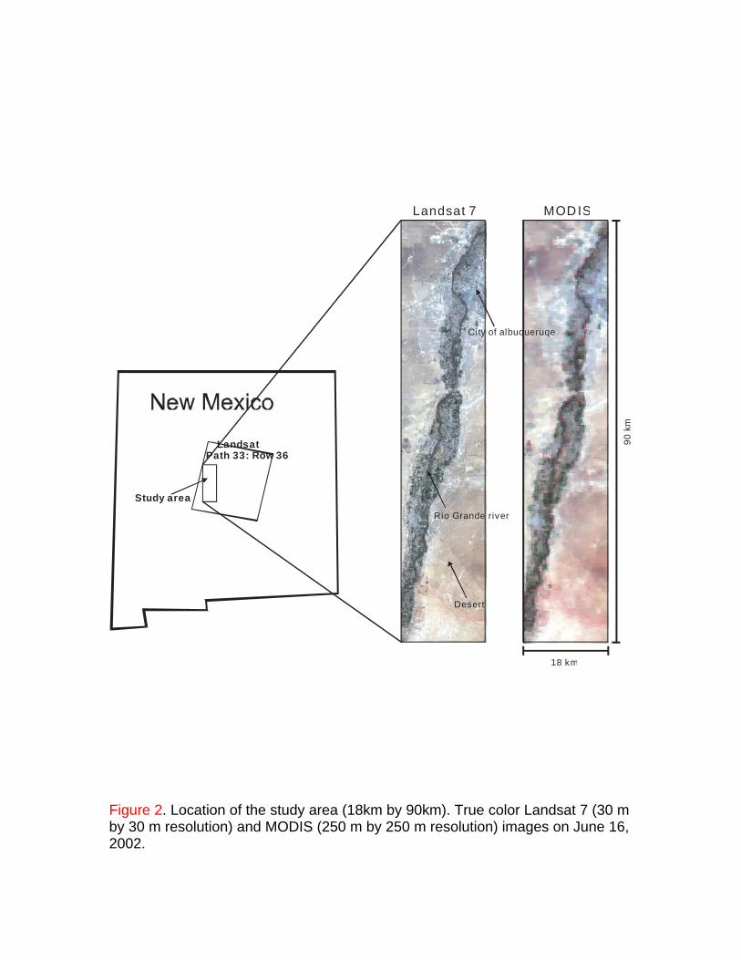
Landsat 7 and Terra MODIS images (Figure 1) on two different dates during the growing 147
season (September 14, 2000 and June 16, 2002) were used to examine the effect of 148
aggregation processes. On these two dates, high quality Landsat 7 and MODIS images 149
were available. The June 16 images are representative for conditions of full vegetative 150
cover at the height of the growing season, while the September 14 images represent 151
somewhat drier conditions towards the end of the growing season. Four satellite images 152
used in this study were georeferenced to match the spatial coordinates as closely as 153
possible. This was done by identifying the several accurate Ground Control Points (e.g. 154
road intersections and agricultural field boundaries) on the images and aligning them to 155
fit on between images. The image used in this study is the subset of the Middle Rio 156
Grande Basin that covers an area of 18 by 90 km. The Middle Rio Grande setting is 157
mainly composed of agricultural fields, riparian forests and surrounding desert areas 158
(Figure 1). 159

8
160
2.2. SURFACE ENERGY BALANCE ALGORITHM FOR LAND (SEBAL) 161
SEBAL is a physically based analytical image processing method that evaluates the 162
components of the energy balance and determines the ET rate as the residual. SEBAL is 163
based on the computation of energy balance parameters from multi spectral satellite data 164
(Bastiaanssen et al., 1998; Morse et al., 2000; Allen et al., 2007). To implement SEBAL, 165
images are needed with information on reflectance in the visible, near-infrared and mid-166
infrared bands, as well as emission in the thermal infrared band. To account for the 167
influence of topographical variations on the energy balance components, a digital 168
elevation model (DEM) with the same spatial resolution as the satellite imagery is also 169
required. The slope and aspect were calculated from DEM using models provided in 170
ERDAS IMAGINE software (ERDAS, 2002). 171
172
The energy balance equation is 173
174
λETHGRn (1) 175
176
where Rn is the net incoming radiation flux density (Wm-2), G is the ground heat flux 177
density (Wm-2), H is the sensible heat flux density (Wm-2), ET is the latent heat flux 178
density (Wm-2), and parameter is the latent heat of vaporization of water (Jkg-1). 179
180
The net radiation (Rn) was computed for each pixel from the radiation balance using 181
surface albedo obtained from short-wave radiation and using emissivity estimated from 182
9
the long-wave radiation (Allen et al., 1998; Bastiaanssen et al., 1998; Morse et al., 2000). 183
Soil heat flux (G) was estimated from net radiation together with other parameters such 184
as normalized difference vegetation index (NDVI), surface temperature and surface 185
albedo (Clothier et al., 1986; Choudhury et al., 1987; Daughtry et al., 1990; Bastiaanssen, 186
2000). Sensible heat flux (H) was calculated from wind speed, estimated surface 187
roughness for momentum transport, and air temperature differences between two heights 188
(0.1 and 2 m) using an iterative process based on the Monin-Obukhov similarity theory 189
(Brutsaert, 1982; Morse et al., 2000; Tasumi, 2003). 190
191
The spatial resolutions of the Landsat 7 bands are 30 and 60 m, compared with 250, 500 192
and 1000m for the MODIS bands (Table 1). Besides the difference in the spatial 193
resolution between Landsat 7 and MODIS, a difference in radiance measurements 194
between the two sensors is expected as a result of slightly different band widths for each 195
sensor. Table 1 also shows the spectral bands of Landsat 7 and MODIS in the visible, 196
near infrared and thermal infrared wavelength regions used for SEBAL application. 197
MODIS bands 1, 2, 3, 4, 6 and 7 are compatible with Landsat 7 bands 3, 4, 1, 2, 5 and 7, 198
respectively. The band widths of MODIS in the visible and near infrared, with the 199
exception of Band 3, are narrower than those of Landsat. This results in different 200
responses from the surface, which in turn may alter the computed surface albedo and 201
vegetation index. 202
203
2.2.1. Brightness temperature 204

10
The major difference in the ET derivation from Landsat and MODIS images was in the 205
surface temperature calculations. SEBAL used one thermal band for surface temperature 206
estimation for Landsat 7 data while two thermal bands were used with MODIS data. 207
208
The temperature detected by a thermal sensor is called the brightness temperature. 209
Radiance data from Landsat 7 and MODIS thermal infrared bands were first converted to 210
brightness temperatures with an inversion of Planck’s equation: 211
1ln12
ln 1
2
52
L
K
K
L
hck
hcTb (2) 212
Tb is the brightness temperature in Kelvin [K], c is the speed of light (2.998 x 10⁸) [ms-1], 213
h is the Planck's Constant (6.626 x 10⁻³⁴) [Js], k is the Boltzmann constant (1.3807 x 10⁻²³) 214
[JK-1], L is the spectral radiance [Wm-2m-1sr-1], is the band effective center 215
wavelength [m] and K1 and K2 are calibration coefficients [Wm-2sr-1m-1] (Table 2). 216
217
2.2.2. Surface temperature 218
For Landsat images the surface temperature (Ts) is estimated using Tb and 0 with the 219
following empirical relationship (Morse et al., 2000). 220
221
25.00
bs
TT (3) 222
223
where 0 = 1.009 + 0.47 ln(NDVI). 224
11
225
For MODIS images the split window technique is used. Split window algorithms take 226
advantage of the differential absorption in two close infrared bands to account for the 227
effects of absorption by atmospheric gases. Several split window algorithms are currently 228
available to derive surface temperature from brightness temperature when multiple 229
thermal bands are available. In this study, the algorithm developed by Price (1984) was 230
applied since Vazquez et al. (1997) determined that it performed better than other 231
algorithms. Ts is given by 232
233
75)1(48)(8.1 323131 TTTTs (4) 234
235
where T31 is the brightness temperature obtained from band31 [K], T32 is the brightness 236
temperature obtained from band 32 [K], = (31+ 32)/2, = 31 –32, 31 is the surface 237
emissivity in band 31 and 32 is the surface emissivity in band 32. 238
Cihlar et al. (1997) developed an algorithm to calculate the surface emissivity from 239
NDVI. 240
(NDVI)..εεΔε ln0134400101903231 (5) 241
where )ln(029.09897.031 NDVI . 242
2.2.3. Daily evapotranspiration 243
In SEBAL, daily ET was interpolated by assuming the instantaneous evaporative fraction 244
(EF) when the satellite was passing over is approximately equal to the daily mean value 245

12
(Shuttleworth et al., 1989; Brutsaert and Sugita, 1992; Crago, 1996; Farah et al., 2004; 246
Gentine et al., 2007). The soil heat flux is assumed to be zero on a daily basis (Kustas et 247
al., 1993). Based on the known value of the instantaneous EF, the daily-averaged net 248
radiation flux, and the soil heat flux over a daily period, daily ET (ET24) can be computed 249
by (Bastiaanssen et al., 1998): 250
251
)(86400 2424
24
GREFET n
(6) 252
253
where HEEEF , 86400 is a constant for time scale conversion, ET24 is daily 254
ET [mmd-1], Rn24 is daily-averaged net radiation [Wm-2] and G24 is daily-averaged soil 255
heat flux [Wm-2]. 256
257
2.3. UP-SCALING (AGGREGATION) PROCESS 258
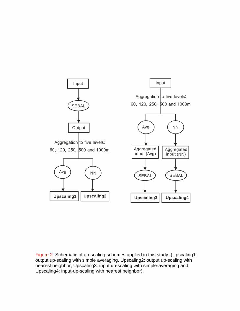
In the up-scaling process, two different procedures were evaluated. The first consisted of 259
applying SEBAL first and then aggregating the output variable (daily ET). The second 260
consisted of aggregating Landsat pixels of input variable (radiance) to obtain pixels at the 261
MODIS scale before SEBAL was applied (Figure 2). If the model is insensitive to an 262
input parameter, aggregating the value with increasing scale will have little influence on 263
model predictions. However, when the model does not operate linearly, the change in 264
data aggregation could increase or decrease model predictions (Quattrochi and Goodchild, 265
1997; French, 2001; Liang, 2004). 266
267

13
Aggregation imagery was obtained by simple averaging and by nearest neighbor 268
selection, and done with ERDAS IMAGINE (Leica Geosystems LLC). The simple 269
averaging resampling method calculated the arithmetic mean over an n by n window. 270
Since a pixel value of satellite imagery is considered to be the integrated value over the 271
corresponding area on the ground, simple averaging is considered appropriate for 272
aggregating remotely sensed images. The simple averaging method smoothes the original 273
data values and therefore produces a “tighter” histogram than the original data set. 274
Furthermore, aggregating a data set by simple averaging generally decreases the variance 275
and also increases the spatial autocorrelation (Anselin and Getis, 1993). 276
The nearest neighbor approach uses the value of the input pixel closest to the center of 277
the output pixel. To determine the nearest neighbor, the algorithm uses the inverse of the 278
transformation matrix to calculate the image file coordinates of the desired geographic 279
coordinate. The pixel value occupying the closest image file coordinate to the estimated 280
coordinate will be used for the output pixel value in the georeferenced image. Unlike 281
simple averaging, nearest neighbor is appropriate for thematic files having data file 282
values based on a qualitative system. One advantage of the nearest neighbor method is 283
that, unlike the simple averaging resampling method, its output values are original input 284
values. The other advantage is that it is easy to compute and therefore fastest to use. 285
However, the disadvantage is that nearest neighbor generates a choppy, "stair-stepped" 286
effect. The image tends to have a rough appearance relative to the original data (Cover 287
and Hart, 1967; Atkinson, 1985; Dodgson, 1997; Bian et al., 1999). 288
14
The aggregation was operated at six levels: 30, 60, 120, 250, 500 and 1000 m pixel sizes. 289
At each level, Landsat scale 30 by 30 m pixels were broken into 10 by 10 m pixels with 290
the same pixel values; the data were then aggregated directly from the 10 m resolution 291
instead of from a previous aggregation. This procedure made it easier to aggregate from 292
the Landsat 30 m pixel size to MODIS 250, 500 and 1000 m pixel sizes. 293
294
3. RESULTS AND DISCUSSION 295
296
3.1. SEBAL CONSISTENCY BETWEEN LANDSAT AND MODIS 297
The SEBAL algorithm was applied to both Landsat 7 and MODIS images acquired on 298
September 14, 2000 and June 16, 2002 and estimated their daily ET rates. In order to 299
check the consistency of SEBAL performance for the different satellite sensors, SEBAL 300
estimated ET from Landsat and MODIS images were compared each other. Spatial 301
distribution of ET maps for visual verification and histograms and basic statistics for 302
quantitative examination were selected. Two approaches were used to inspect the ET 303
estimation difference between two different satellite sensors: one is a difference image 304
(pixel-by-pixel difference between Landsat and MODIS estimates), while the other was a 305
relative difference image (absolute value of the pixel difference was divided by the 306
MODIS derived pixel value). Basic statistics of the difference and relative difference 307
images were also computed to quantify the discrepancy between Landsat and MODIS 308
estimates. 309
310
3.1.1 Comparison between Landsat (30m) and MODIS (250m) estimated ET 311

15
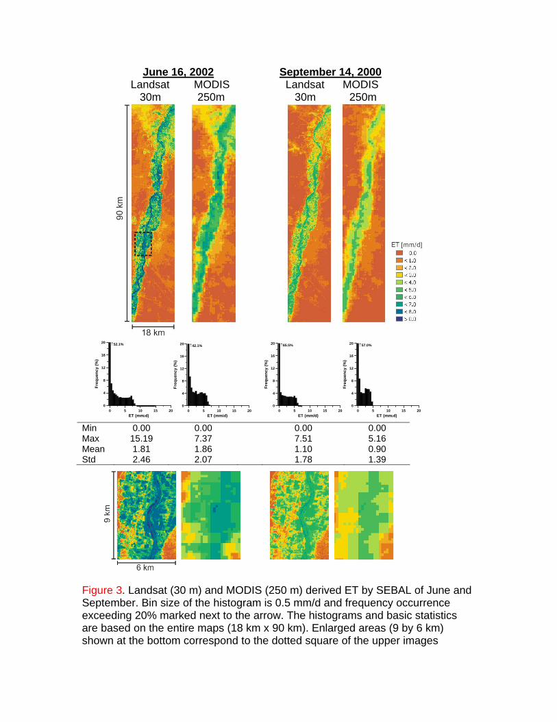
Figure 3 shows that the June image taken during the summer has significantly higher ET 312
rates than the September image taken in the early fall. All of the ET images clearly show 313
high ET rates in the irrigated fields and riparian areas along the Rio Grande Valley, while 314
low ET rates are shown in the surrounding desert areas and bare soils. The city of 315
Albuquerque has a somewhat higher ET rate than surrounding desert areas due to urban 316
and residential vegetations. 317
318
The disparate spatial resolutions of Landsat- and MODIS-based ET images result in some 319
differences in ET distribution, as may be expected. Many small areas (length scale on the 320
order of 10 to 100 m) with high ET rates along the river are captured well in the Landsat-321
based ET map with a spatial resolution of 30 m. These peak ET rates are averaged out, 322
however, on the MODIS derived ET map with a spatial resolution of 250 m. Figure 3 323
shows that MODIS derived ET distributions have a tighter and taller histogram and fewer 324
pixels have close to zero (0.0 to 0.5) ET than the histogram from Landsat imagery. In the 325
table of basic statistics in Figure 3, the ET map derived from the Landsat 7 image shows 326
a higher maximum and standard deviation than the one derived from the MODIS images. 327
However, the mean values of Landsat- and MODIS-based ET images are very similar. 328
The minimum value of ET in each image equals to zero. 329
330
Difference images between the Landsat-based ET at 30m resolution and MODIS-based 331
ET at 250m resolution show how these products are dissimilar to each other (Figure 4). 332
Each difference image was produced by subtracting MODIS-based ET from Landsat-333
based ET [ETLandsat – ETMODIS], with brown-colored pixels in the difference map in Figure 334
16
4 representing points where the MODIS-based ET is significantly higher than Landsat-335
based ET. Blue-colored pixels represent points where the ET from Landsat is 336
significantly higher than the ET from MODIS imagery. Areas with apparently high ET 337
differences (> +2.0 or < -2.0 mm/d) shown as brown or blue, are observed along the 338
boundary between Rio Grande River riparian areas and surrounding deserts. These high 339
differences are mostly due to (1) disagreement in image georeferencing between the 340
Landsat and MODIS imagery and (2) differences resulting from subtracting the ET value 341
of a large (250m) MODIS based pixel from that of a small (30m) Landsat based pixel. 342
343
It is not trivial to generate georeferenced imagery with error of less than one pixel 344
(Eugenio and Marqués, 2003). The georeferencing of two maps with spatial resolutions 345
differing an order of magnitude is especially difficult (Liang et al., 2002). One or two 346
pixels of georeferencing disagreement can cause abrupt ET changes at the boundaries 347
between riparian (high ET) and desert (low ET) areas. The effect of different pixel sizes 348
is clearly demonstrated with the brown and blue pixels located along the sudden 349
transition from riparian area to desert. The brown-colored pixels (ET difference < -2 350
mm/d) are located in the desert and result from subtracting a large MODIS pixel located 351
partially in the riparian area with relatively high ET from a small Landsat pixel located in 352
the desert with zero ET. The blue-colored pixels (ET difference > 2 mm/d) are located in 353
the riparian area and result from subtracting a large MODIS pixel located partially in the 354
desert from a riparian area located small Landsat pixel. 355
356

17
Basic statistics (mean and standard deviation) allow a quantitative means of comparison 357
and evaluation. Positive and negative differences due to georeferencing disagreement 358
between two images tend to cancel each other in these calculations since they occur in 359
opposite directions at both sides of the transgression from riparian to desert area. 360
Therefore the mean and standard deviation of each difference image were calculated 361
based on the “absolute” difference between Landsat- and MODIS-based ET images. For 362
both study dates, the mean and standard deviation of difference between the Landsat and 363
MODIS-based ET are within 1.0 mm/day. Basic statistics in Figure 4 show that the 364
September images have a slightly lower mean difference and standard deviation than the 365
June images. However, this does not imply that the September Landsat- and MODIS-366
based ET images agree better than June images. The difference in basic statistics is 367
caused by the smaller values of the mean and standard deviation of ET rates in the 368
September images. 369
370
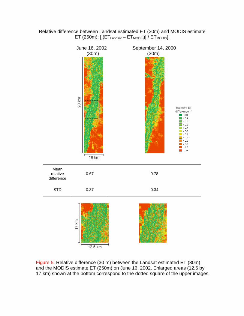
Relative difference images were produced as well by dividing the absolute difference 371
image by the MODIS derived ET image [|(ETLandsat – ETMODIS)| /ETMODIS] (Figure 5). The 372
relative difference value ranges from zero to infinity. The infinity values occur when the 373
MODIS-based ET is much smaller than the Landsat-based ET. The infinity values were 374
constrained to 1.0 and pixels having zero values either in the MODIS-based ET or in the 375
Landsat-based ET image are also assigned to 1.0 as relative difference. Most of the pixels 376
having 1.0 (red-colored) relative difference are located in the desert area. One interesting 377
point is that the quite a few pixels having 1.0 as relative difference are found along the 378
transition zone between riparian and desert areas. Those pixels result from 30 m Landsat 379

18
pixels having high ET inside 250 m coarse resolution of MODIS pixels having low ET 380
(Figure 5). 381
382
Figure 6 presents three dimensional graphs of the relationship between relative difference 383
and daily ET rate on both June and September images. Both graphs in Figure 6 show that 384
large relative difference predominantly occur in areas having low ET while areas having 385
ET such as greater than 3 mm/d exhibit relative differences of about less than 0.4. 386
However, there are some points having 1.0 relative difference with daily ET greater than 387
2.0 mm/d. These points are resulted from pixels having significant difference between 388
Landsat and MODIS derived ET and mainly due to georeferencing disagreement between 389
Landsat and MODIS satellite images. These questionable points are mostly located in the 390
boundary area between riparian and surrounding desert. 391
392
3.2. ANALYSIS OF UP-SCALING EFFECTS 393
The spatial distribution and its statistical features were evaluated and compared among 394
the four different up-scaling methods across the five aggregation levels. Output up-395
scaling aggregated the SEBAL estimated daily ET rates either with simple averaging or 396
the nearest neighbor resampling method. The resultant aggregated ET map may represent 397
the best estimate of ET at the coarser resolution, since the aggregated ET was derived 398
directly by aggregation of the fine resolution ET data. For input up-scaling, since the 399
radiometric observations (radiance) or SEBAL model inputs were aggregated, one 400
expects to retrieve the best estimate of a radiometric observation at the coarser 401

19
resolutions. These aggregated data were used as input to the SEBAL model and 402
calculated daily ET. 403
404
The different up-scaling methodologies were evaluated by: (1) spatial distribution of 405
aggregated imagery by four different schemes at each aggregation level to evaluate the 406
changes in spatial pattern after aggregation, and (2) histograms and basic statistics of the 407
aggregated data for different up-scaling schemes at all levels. The spatial details lost 408
during aggregation were considered to be the difference between original image and up-409
scaled image. In this study difference images were created by subtracting the up-scaled 410
pixels from the original pixels of the Landsat- or MODIS-based ET estimates. While 411
relative difference images were produced by dividing the absolute difference by the 412
original Landsat- and MODIS-based ET images. The statistical and spatial characteristics 413
of differences were evaluated by analyzing the spatial distribution of differences as well 414
as the mean and standard deviation of absolute differences. 415
416
3.2.1. Effect of aggregation 417
Spatial and statistical characteristics of up-scaled products from June and September 418
Landsat-based ET maps at 30m resolution to five aggregation levels are presented in 419
Figures 7 –10. Figure 7 presents ET maps from output up-scaling using simple averaging 420
resampling on June 16, 2002, at spatial resolutions of 60, 120, 250, 500 and 1000m. This 421
method produces the most statistically and spatially predictable behavior. The least 422
predictable – but still acceptable – behavior is produced by input up-scaling using nearest 423
neighbor resampling. An example for June 16, 2002 is presented in Figure 8. Figures 9 424

20
and 10 present the histograms and statistics for the different up-scaling methods on, 425
respectively, June 16, 2002 and September 14, 2000. Although spatial detail was lost 426
with the increase in pixel size, the overall spatial distribution of ET of each aggregated 427
map (for example Figures 7 and 8) was in agreement with the original ET maps in Figure 428
3. 429
430
All histograms of ET distribution (Figures 9 and 10) show the dominance of close to zero 431
ET values and this frequency decreases a few percent (3.4 to 1.3%) with pixel size only 432
when output up-scaling with simple averaging was applied. This feature might be 433
explained by the observation that desert areas along the riparian corridors are classified to 434
have zero ET in fine resolution of 30m. However, these desert areas are easily mixed 435
with riparian areas when applying simple averaging, while nearest neighbor resampling 436
schemes hardly affect the frequencies in the histogram since nearest neighbor produces a 437
subset of the original data. The 60 and 120m pixel sized histograms in Figures 9 – 10 438
exhibit an almost constant frequency occurrence of 2.0% for June imagery and 3.0% for 439
September imagery over ET rates ranging from 2.5 to 7.5 mm/d and from 1.0 to 5.0 440
mm/d, respectively. This constant frequency changes into a concave down shape as pixel 441
size is increased further with simple averaging resampling in both output and input up-442
scaling. That is, the frequency of pixels having 5 – 6 mm/d ET increases but the 443
frequency of pixels having 3 – 4 mm/d decreases with simple averaging is applied. Pixels 444
having 5 – 6 mm/d of ET in this study area are mainly surface water, agricultural fields 445
and riparian vegetation pixels located along the Rio Grande riparian corridor. There are 446
pixels having 3 – 4 mm/d of ET located inside of the riparian corridor as well as in the 447

21
transition zone between riparian and surrounding desert. These pixels are mostly located 448
along the transition zone between riparian areas and surrounding deserts areas and 449
adjacent to the Rio Grande River. These pixels have low ET, but when averaged with 450
adjacent higher ET pixels the contrast disappears. However, histograms from nearest 451
neighbor resampling stayed rather consistent in shape at each resolution. 452
453
The basic statistics and histograms also show the statistical changes through aggregation. 454
With either output up-scaling or input up-scaling, the mean values of the simple 455
averaging and nearest neighbor images remain essentially constant across all aggregation 456
levels in both days. However, ET maps derived using nearest neighbor show a more 457
“blocky” pattern than those derived using from simple averaging (for example Figures 7 458
and 8). This difference in spatial distribution is due to the fact that simple averaging 459
decreases the standard deviation with increasing pixel size, while the standard deviation 460
from nearest neighbor aggregation stays fairly constant across all aggregation levels. 461
462
The differences in aggregation procedures between simple averaging and nearest 463
neighbor cause the fundamental difference in statistics of the aggregated data. The simple 464
averaging method aggregates based on data values, and the resulting values are confined 465
to the mid range. However, the nearest neighbor resampling is based on location, its pixel 466
value varying with the location of central pixels in new coordinates as the pixel size 467
changes. Therefore, the aggregated results are a systematically sampled subset of the 468
original data, and their values are expected to be less confined. This explains the 469
somewhat larger data ranges for the nearest neighbor resampling method, but the mean of 470

22
the data does not change significantly. Many regional-scale hydrological process models 471
require input parameters over a large area. Direct area averaging technique has often 472
been used to generate the regional-scale model input parameters (Shuttleworth, 1991; 473
Chehbouni and Njoku, 1995; Croley et al., 2005; Maayar and Chen, 2006). For example, 474
direct averaged values of air temperature, precipitation, humidity, surface roughness 475
length and so on were used as input parameters in hydrologic models (Brown et al., 1993; 476
Maayar and Chen, 2006). However, the standard deviation of the data set decreases as the 477
aggregation level increases, therefore users need to check the sensitivity of the range of 478
the variable of the model prior to applying direct averaging for data aggregation. 479
480
In fact, the SEBAL algorithm is nonlinear; that is the mean aggregated ET (output up-481
scaled) at any given resolution does not equal the modeled ET value of an aggregated 482
input value (input up-scaled). However, as demonstrated by visual examination of the 483
spatial distribution of ET in Figures 7 10, the contrast as well as the basic patterns (high 484
and low values and their relative locations) of ET between output up-scaling and input 485
up-scaling show a slight disagreement. A slightly higher mean and standard deviation 486
was found in the results from input up-scaling with simple averaging than from output 487
up-scaling with simple averaging; however there is almost no difference between input 488
and output up-scaling when applying the nearest neighbor method. Overall, statistical and 489
spatial characteristics produced by input up-scaling show relatively good agreement with 490
those of the output up-scaling method. 491
492

23
3.2.2. Difference of aggregated data versus original Landsat (30m) and MODIS 493
(250m) estimated ET 494
First, aggregation difference was examined by comparing aggregated maps with the 495
original ET map at 30m resolution derived from Landsat imagery. Tables 3 and 4 present 496
the basic statistics of difference and relative difference against original Landsat derived 497
ET on June 16, 2002 and September 14, 2000 produced by four different up-scaling. The 498
mean values of absolute difference and relative difference range from 0.14 to 0.63 mm/d 499
and from 0.55 to 0.82, respectively. 500
The mean and standard deviation values of absolute difference from September image are 501
smaller than those from June image. The smaller mean difference and standard deviation 502
is explained by the smaller values of the ET rates in the September image. Mean values 503
of absolute difference from output up-scaled maps are similar with those from input up-504
scaled maps; however consistently higher standard deviations are found in input up-505
scaled maps (Tables 3 – 4). This result confirms that aggregated model output data 506
provide the best estimate of model output at the coarser resolution. 507
508
The mean and standard deviation of the absolute differences also increase with pixel size. 509
This is mainly due to the mixed pixel effect. Since aggregation tends to average out the 510
small surface features, the difference between aggregated imagery and the original fine 511
resolution imagery increases with aggregation levels. One interesting note is that the 512
mean of the relative difference increase with pixel size, however standard deviation 513
actually slightly decreases with pixel size. In this study relative difference is bounded to 514
be not greater than 1.0. Therefore, as mean values increase to approach 1.0, the standard 515

24
deviation of absolute difference actually decreases with increasing relative difference. 516
Based on the mean and standard deviation of the absolute difference and relative 517
difference, although the difference increases with aggregation levels, the ET of the 518
original images seems to be better preserved from the output up-scaling than input up-519
scaling. 520
521
Both of the 3D frequency plots in Figure 11 between up-scaled ET and its relative 522
difference against Landsat-based ET show patterns similar to those in Figure 6. That is, 523
relative difference decreases with ET. However, points having 1.0 relative difference 524
with daily ET greater than 1.0 mm/d are greatly diminished in Figure 11. In particular, 525
the top portion of Figure 11, which shows the relative difference between the output up-526
scaled ET and the ET obtained from simple averaging, shows very few of these 527
questionable points. In the bottom portion of Figure 11, which shows the relative 528
difference between the input up-scaled ET and the nearest neighbor up-scaled ET, there 529
are some points with a relative difference of 1.0, but there are far fewer such points than 530
in Figure 6. This indicates that there are fewer georeferencing disagreements between 531
Landsat-derived ET and output up-scaled ET than the one between Landsat and MODIS 532
images. 533
534
Next, we compare aggregation differences by comparing up-scaled maps at 250m 535
resolution with the original ET map from MODIS. This requires that we first examine 536
which aggregation scheme produces the best match with the original MODIS-based ET 537
and then check the quality of the different aggregation schemes. Landsat-based ET maps 538

25
at 30 m resolution were aggregated into 250 m resolution maps by applying the four 539
different aggregation schemes already presented in Figure 2. Table 5 show the basic 540
statistics of the absolute difference and relative difference of images from the four 541
different up-scaling schemes at 250m resolution compared with MODIS-based ET of 542
June and September. 543
544
The mean and standard deviation of absolute difference and relative difference from 545
output up-scaling with the simple averaging map are smaller than the one from input up-546
scaling (Table 5). Also the simple averaging method generates smaller absolute 547
difference and relative difference than the nearest neighboring method. This implies that 548
output up-scaling with simple averaging map has best agreement with MODIS derived 549
ET. No difference between output and input up-scaling is found from the nearest 550
neighbor aggregation method. As shown in the previous section, the maximum and 551
standard deviation of the ET maps produced by simple averaging are decreased as data 552
were aggregated to 250m resolution. However, the nearest neighbor aggregation method 553
generated images having a similar maximum and standard deviation to the original image 554
(Figures 9 10). This explains why the mean and standard deviation of absolute 555
difference between aggregated Landsat ET image using simple averaging and MODIS-556
based ET are smaller than from nearest neighbor (Table 5). 557
558
Although the difference increases with aggregation levels, the ET of 559
the original images seems to be better preserved with output up-scaling than 560
26
with input up-scaling. Out of the four different up-scaling procedures, output up-scaling 561
with simple averaging performs best. However, all four aggregation schemes are still 562
acceptable since the mean and standard deviation values of absolute difference are all less 563
than those from the original Landsat ET imagery in Figure 4. 564
565
3.3. COMPARISON OF SEBAL UNCERTAINTY WITH UP-SCALING EFFECTS 566
567
As mentioned in Section 1, it has been reported that SEBAL daily ET estimates agree 568
with ground observation with an accuracy of 10%.The great strength of the SEBAL is 569
due to its internal calibration procedure that eliminates most of the bias in latent heat flux 570
at the expense of increased bias in sensible heat flux (Allen et al., 2007; Hong, 2008). 571
572
In order to examine the difference among up-scaling schemes, the relative difference 573
between up-scaled ET images at 120 and 1000m resolutions are calculated and histogram 574
and descriptive statistics are shown in Figure 12. Relative difference is calculated 575
between Upscaling2, 3 or 4 against Upscaling1 (Figure 2) as [|(ET upscaling2, 3 or 4 – 576
ETupscaling1)| /ET upscaling1]. Up-scaling1 (output simple averaging) is taken as reference 577
since output simple averaging generates the best matched up-scaled map with respect to 578
the MODIS-derived ET map (Table 5). As shown in Figure 1, the study area includes 579
surrounding desert where soil moisture is little thus ET is very small. Since area having 580
very low ET can easily introduce very high relative difference and moreover it is difficult 581
to precisely estimate ET in desert area anyhow, the area having less than 1mm/day is 582
27
excluded in this analysis. The portion of area having less than 1mm/day covers about 583
50% of whole study area. 584
585
As shown in Figure 12, first, mean relative difference increases with pixel spatial 586
resolution, and second, relative difference between simple averaging and nearest 587
neighboring resampling (Upscaling1-Upscaling2 and Upscaling1-Upscaling4) has a lot 588
higher mean and standard deviation than the one between two simple averaging schemes 589
(Upscaling1-Upscaling3). This simply indicates that as pixel size increases, the difference 590
between simple averaging and nearest neighboring resampling increases. However, mean 591
relative difference between Upscaling1 and Upscaling3 (input simple averaging) in both 592
120m and 1000m resolution are all less than 10% which is smaller than the magnitude of 593
SEBAL uncertainty. A little difference between output and input up-scaling implies that 594
SEBAL is close to linearity model and that is due to its internal calibration procedure 595
(dT-Ts relationship). Another interesting point is that for the 1000m resolution histograms 596
of Upscaling1-Upscaling2 and Upscaling1-Upscaling3, considerable data points have 597
relative difference greater than 10% and especially lots of pixels (15% frequency) have 598
relative difference greater than 90%. Those areas having >90% relative difference are 599
mainly located along the boundary between riparian and desert areas. These pixels in the 600
boundary area are mixed with riparian (high ET) and desert (low ET), thus the difference 601
between up-scaled ET map by simple averaging and nearest neighbor resampling is 602
significant and causes very high relative difference. 603
604

28
Based on the result of relative difference analysis, the difference between simple 605
averaging and nearest neighbor is a lot bigger than the uncertainty of the SEBAL 606
procedure. Therefore, users have to aware of the difference and are careful to select 607
appropriate up-scaling scheme for their research. 608
609
610
4. CONCLUSIONS 611
612
Daily evapotranspiration rates were predicted using the SEBAL algorithm from Landsat 613
7 and MODIS imagery. The objectives of this study were to test the consistency of the 614
SEBAL algorithm for the different satellite sensors and to investigate the effect of 615
various proposed aggregation procedures. 616
617
Although ET maps derived from the Landsat 7 images showed higher maximum and 618
standard deviation values than those derived from the MODIS images, the mean values of 619
Landsat- and MODIS-based ET images were very similar. Discrepancy in direct pixel-620
by-pixel comparison between Landsat- and MODIS-based ET was due to mainly 621
georeferencing disagreement as well as the inherent differences in spatial, spectral and 622
radiometric resolutions between imagery from the different satellite sensors. 623
624
The output up-scaling scheme produced slightly better ET maps than the input up-scaling 625
scheme. Both simple averaging and nearest neighbor resampling methods can preserve 626
the mean values of the original images across aggregation levels. However, the simple 627

29
averaging resampling method resulted in decreasing standard deviation values as the 628
resolution coarsened, while the standard deviation did not change across aggregation 629
levels with the nearest neighbor resampling method. For difference analysis, large 630
relative differences predominantly occur in areas having low ET (desert and bare soil) 631
while areas having high ET (agricultural field and riparian vegetation) exhibit small 632
relative differences. Out of the four different up-scaling procedures proposed in this study, 633
output up-scaling with simple averaging performs best. However, other aggregation 634
schemes are still acceptable. 635
636
Results of the relative difference analysis among up-scaling schemes show that a little 637
difference between output and input up-scaling is found. However, there significant 638
difference exists between simple averaging and nearest neighbor and its difference is a lot 639
bigger than the uncertainty of the SEBAL procedure. 640
641
642
5. ACKNOWLEDGEMENT 643
644
The following sponsors have contributed to this study: U.S. Department of Agriculture, 645
CSREES grant No.: 2003-35102-13654 and NSF EPSCoR grant EPS-0132632. 646
647
6. REFERENCES 648
Allen, R.G., M. Tasumi, and R. Trezza. 2007. Satellite-based Energy Balance for 649 Mapping Evapotranspiration with Internalized Calibration (METRIC) – Model. 650 Journal of Irrigation and Drainage Engineering, ASCE 133:380-394. 651

30
Allen, R.G., L.S. Pereira, D. Raes, and M. Smith. 1998. Crop evapotranspiration. FAO 652 Irrigation and drainage paper 56, FAO. Rome. 653
Anselin, L., and A. Getis. 1993. Spatial statistical analysis and geographic information 654 systems Springer-Verlag, New York. 655
Atkinson, P.M. 1985. Preliminary Results of the Effect of Resampling on Thematic 656 Mapper Imagery. ACSM-ASPRS Fall Convention Technical Papers:929-936. 657
Bastiaanssen, W.G.M. 2000. SEBAL-based sensible and latent heat fluxes in the Irrigated 658 Gediz Basin, Turkey. Journal of Hydrology 229:87-100. 659
Bastiaanssen, W.G.M., M. Menenti, R.A. Feddes, and A.A.M. Holtslag. 1998. A remote 660 sensing surface energy balance algorithm for land (SEBAL). Part 1: Formulation. 661 Journal of Hydrology 212-213:198-212. 662
Bastiaanssen, W.G.M., E.J.M. Noordman, H. Pelgrum, G. Davids, B.P. Thoreson, and 663 R.G. Allen. 2005. SEBAL model with remotely sensed data to improve water-664 resources management under actual field conditions. Journal of Irrigation and 665 Drainage Engineering 131:85-93. 666
Bian, L. 1997. Multiscale nature of spatial data in scaling up environment models CRC 667 Press, Inc. 668
Bian, L., R. Butler, D.A. Quattrochi, and P.M. Atkinson. 1999. Comparing effects of 669 aggregation methods on statistical and spatial properties of simulated spatial data. 670 Photogrammetry and Remote Sensing 65:73-84. 671
Brown, D.G., L. Bian, and S.J. Walsh. 1993. Response of a distributed watershed erosion 672 model to variations in input data aggregation levels. Computers and Geosciences 673 19:499-509. 674
Brutsaert, W. 1982. Evaporation into the atmosphere D. Reidel Pub. Co., Dordrecht, The 675 Netherlands. 676
Brutsaert, W., and M. Sugita. 1992. Application of self-preservation in the diurnal 677 evolution of the surface energy budget to determine daily evaporation. Journal of 678 Geophysical Research 97:18,377-18,382. 679
Carmel, Y. 2004. Controlling data uncertainty via aggregation in remotely sensed data. 680 IEEE Transaction on Geoscience and Remote Sensing Letters 1:39-41. 681
Carmel, Y., J. Dean, and C.H. Flather. 2001. Combining location and classification error 682 sources of estimating multi-temporal database accuracy. Photogrammetric 683 Engineering and Remote Sensing 67:865-872. 684
Chehbouni, A., and E.G. Njoku. 1995. Approaches for averaging surface parameters and 685 fluxes over heterogeneous terrain. Journal of Climate 8:1386-1393. 686
Choudhury, B.J., S.B. Idso, and R.J. Reginato. 1987. Analysis of an empirical model for 687 soil heat flux under a growing wheat crop for estimating evaporation by an 688 infrared-temperature-based energy balance equation. Agriculture and Forest 689 Meteorology 39:283-297. 690
Cihlar, J., H. Ly, Z. Li, J. Chen, H. Pokrant, and F. Hung. 1997. Multi-temporal, Multi-691 channel AVHRR data sets for land biosphere studies – Artifacts and corrections. 692 Remote Sensing of Environment 60:35-57. 693
Clothier, B.E., K.L. Clawson, J. P.J. Pinter, M.S. Moran, R.J. Reginato, and R.D. Jackson. 694 1986. Estimation of soil heat flux from net radiation during growth of alfalfa. 695 Agricultural and Forest Meteorology 37:319-329,. 696
31
Cover, T., and P. Hart. 1967. Nearest neighbor pattern classification. IEEE Transactions 697 on Information Theory 13:21- 27. 698
Crago, R.D. 1996. Conservation and variability of the evaporative fraction during the 699 daytime. Journal of Hydrology 180:173-194. 700
Croley, I., T. E., C. He, and D.H. Lee. 2005. Distributed-Parameter Large Basin Runoff 701 Model. II: Application. Journal of Hydrologic Engineering 10:182-191 702
Dai, X.L., and S. Khorram. 1998. The effects of image misregistration on the accuracy of 703 remotely sensed change detection. IEEE Transaction on Geoscience and Remote 704 Sensing 36:1566-1577. 705
Daughtry, C.S., W.P. Kustas, M.S. Moran, R.D. Jackson, and J. Pinter. 1990. Spectral 706 estimates of net radiation and soil heat flux. Remote Sensing of Environment 707 32:111-124. 708
De Cola, L. 1994. Simulating and mapping spatial complexity using multi-scale 709 techniques. International Journal of Geographical Information Systems 8:411-427. 710
Dodgson, N.A. 1997. Quadratic interpolation for image resampling. IEEE Transactions 711 on Image Processing 6:1322-1326. 712
Ebleringer, J.R., and C.B. Field. 1993. Scaling Physiological Processes, Leaf to Globe 713 Academic Press, Inc., New York. 714
ERDAS. 2002. Field Guide 6th ed. Atlanta, Georgia, ERDAS Inc. 715 Eugenio, F., and F. Marqués. 2003. Automatic Satellite Image Georeferencing Using a 716
Contour-Matching Approach. IEEE Transactions on Geoscience and Remote 717 Sensing 41:2869-2880. 718
Farah, H.O., W.G.M. Bastiaanssen, and R.A. Feddes. 2004. Evaluation of the temporal 719 variability of the evaporative fraction in a tropical watershed. International 720 Journal of Applied Earth Observation and Geoinformation 5:129-140. 721
French, A.N. 2001. Scaling of surface energy fluxes using remotely sensed data. PhD 722 Thesis, University of Maryland, College Park. 723
French, A.N., T.J. Schmugge, and W.P. Kustas. 2002. Estimating evapotranspiration over 724 El Reno, Oklahoma with ASTER imagery. Agronomie 22:105-106. 725
Gentine, P., D. Entekhabi, A. Chehbouni, G. Boulet, and B. Duchemin. 2007. Analysis of 726 evaporative fraction diurnal behaviour. Agricultural and Forest Meteorology 727 143:13-29. 728
Gupta, V.K., I. Rodriguez-Iturbe, and E.F. Wood. 1986. Scale Problems in Hydrology D. 729 Reidel Publishing Company, Boston. 730
Hendrickx, J.M.H., and S.-H. Hong. 2005. Mapping sensible and latent heat fluxes in arid 731 areas using optical imagery. Proceedings of International Society for Optical 732 Engineering, SPIE 5811:138-146. 733
Hong, S.-H. 2008. Mapping regional distributions of energy balance components using 734 optical remotely sensed imagery. PhD. Dissertation. Dept. of Earth & 735 Environmental Science (Hydrology Program), New Mexico Institute of Mining 736 and Technology, Socorro, NM, USA. 737
Hong, S.-H., J.M.H. Hendrickx, and B. Borchers. 2005. Effect of scaling transfer 738 between evapotranspiration maps derived from LandSat 7 and MODIS images. 739 Proceedings of International Society for Optical Engineering, SPIE 5811:147-158. 740

32
Kustas, W.P., C.S.T. Daughtry, and P.J.V. Oevelen. 1993. Analytical treatment of the 741 relationships between soil heat flux/net radiation ratio and vegetation indices. 742 Remote Sensing and Environment 46:319-330. 743
Lam, N., and D.A. Quattrochi. 1992. On the issues of scale, resolution, and fractal 744 analysis in the mapping sciences. Professional Geographer 44:88-98. 745
Lhomme, J.-P. 1992. Energy balance of heterogeneous terrain: Averaging the controlling 746 parameters. Agricultural and Forest Meteorology 61:11-21. 747
Li, B., and R. Avissar. 1994. The impact of spatial variability of land-surface 748 characteristics on land-surface fluxes. Journal of Climate 7:527-537. 749
Liang, S. 2000. Numerical experiments on spatial scaling of land surface albedo and leaf. 750 area index. Remote Sensing Reviews 19:225–242. 751
Liang, S. 2004. Quantitative Remote Sensing of Land Surfaces John Wiley and Sons, Inc. 752 Liang, S., H. Fang, M. Chen, C.J. Shuey, C. Walthall, C. Daughtry, J. Morisette, C. 753
Schaaf, and A. Strahler. 2002. Validating MODIS land surface reflectance and 754 albedo products: methods and preliminary results. Remote Sensing of 755 Environment 83:149-162. 756
Maayar, M.E., and J.M. Chen. 2006. Spatial scaling of evapotranspiration as affected by 757 heterogeneities in vegetation, topography, and soil texture. Remote Sensing of 758 Environment 102:33-51. 759
Mark, D.M., and P.B. Aronson. 1984. Scale dependent fractal dimensions of topographic 760 surfaces: An empirical investigation with applications in geomorphology and 761 computer mapping. Mathmatical Geology 16:671-683. 762
Mecikalski, J.R., G.R. Diak, M.C. Anderson, and J.M. Norman. 1999. Estimating fluxes 763 on continental scales using remotely-sensed data in an atmospheric-land exchange 764 model. Journal of Applied Meteorology 38:1352-1369. 765
Mengelkamp, H.-T., F. Beyrich, G. Heinemann, F. Ament, J. Bange, F. Berger, J. 766 Bösenberg, T. Foken, B. Hennemuth, C. Heret, S. Huneke, K.-P. Johnsen, M. 767 Kerschgens, W. Kohsiek, J.-P. Leps, C. Liebethal, H. Lohse, M. Mauder, W. 768 Meijninger, S. Raasch, C. Simmer, T. Spieß, A. Tittebrand, J. Uhlenbrock, and P. 769 Zittel. 2006. Evaporation Over A Heterogeneous Land Surface. Bulletin of the 770 American Meteorological Society 87:775-786. 771
Morse, A., M. Tasumi, R.G. Allen, and W.J. Kramer. 2000. Application of the SEBAL 772 methodology for estimating consumptive use of water and streamflow depletion 773 in the Bear river basin of Idaho through remote sensing. Final report submitted to 774 the Raytheon Systems Company, Earth Observation System Data and Information 775 System Project, by Idaho Department of Water Resources and University of Idaho. 776
Nellis, M.D., and J.M. Briggs. 1989. The effect of spatial scale on Konza landscape 777 classification using textural analysis. Landscape Ecology 2:93-100. 778
Nishida, K., R.R. Nemani, S.W. Running, and J.M. Glassy. 2003. An operational remote 779 sensing algorithm of land surface evaporation. Journal of Geophysical Research 780 108 (D9):doi:10.1029/2002JD002062. 781
Price, J.C. 1984. Land surface temperature measurements from the split window channel 782 of the NOAA 7 Advanced Very High Resolution Radiometer. Journal of 783 Geophysical Research 89:7231-7237. 784
Quattrochi, D.A., and M.F. Goodchild. 1997. Scale, multiscaling, remote sensing, and 785 GIS Lewis Publishers, New York. 786
33
Seguin, B., J.-P. Lagouarde, and M. Saranc. 1991. The assessment of regional crop water 787 conditions from meteorological satellite thermal infrared data. Remote Sensing of 788 Environment 35:141-148. 789
Seyfried, M.S., and B.P. Wilcox. 1995. Scale and the nature of spatial variability: Field 790 examples having implications for hydrologic modeling. Water Resources 791 Research 31:173 - 184. 792
Shuttleworth, W.J. 1991. The modllion concept. Review of Geophysics 29:585-606. 793 Shuttleworth, W.J., R.J. Gurney, A.Y. Hsu, and J.P. Ormsby. 1989. The variation in 794
energy partition at surface flux sites. Proceedings of the IAHS Third International 795 Assembly, Baltimore, MD. 186:67-74. 796
Stoms, D. 1992. Effects of habitat map generalization in biodiversity assessment. 797 Photogrammetric Engineering and Remote Sensing 58:1587-1591. 798
Tasumi, M. 2003. Progress in operational estimation of regional evapotranspiration using 799 satellite imagery. Ph.D., University of Idaho, Moscow, Idaho. 800
Townshend, J.R.G., C.O. Justice, C. Gurney, and J. McManus. 1992. The impact of 801 misregistration on change detection. IEEE Transaction on Geoscience and 802 Remote Sensing 30:1054-1060. 803
Turner, M.G., R.V. O'Neil, R.H. Gardner, and B.T. Milne. 1989. Effects of changing 804 spatial scale on the analysis of landscape pattern. Landscape Ecology 3:153-162. 805
Van Rompaey, A.J.J., G. Govers, and M. Baudet. 1999. A strategy for controlling error of 806 distributed environmental models by aggregation. International Journal of 807 Geographical Information Science 13:577-590. 808
Vazquez, D.P., F.J. Olmo Reyes, and L.A. Arboledas. 1997. A comparative study of 809 algorithms for estimating land surface temperature from AVHRR data. Remote 810 Sensing of Environment 62:215-222. 811
Vieux, B.E. 1993. DEM Aggregation and smoothing effects on surface runoff modeling. 812 Journal of Computing in Civil Engineering 7:310-338. 813
Wolock, D.M., and C.V. Price. 1994. Effects of digital elevation model map scale and 814 data resolution on a topography-based watershed model. Water Resources 815 Research 40:3041-3052. 816
Zhang, W., and D.R. Montgomery. 1994. Digital elevation model grid size, landscape 817 representation, and hydrologic simulations. Water Resources Research 30:1019-818 1028. 819
820 821

Table 1. Band spatial resolutions (m] and wavelengths (μm) of Landsat 7 and MODIS sensors.
Band number
Sensors
1
2
3 4
5#
6
7
31
32
Pixel size [m]
30
30
30
30
30
60
30
NA*
NA*
Landsat 7
Band width [μm]
0.45
– 0.51
0.52
– 0.60
0.63
– 0.69
0.75
– 0.9
1.55
– 1.75
10.4
– 12.5
2.09
– 2.35
NA*
NA
Pixel size [m]
250
250
500
500
500
500
500
1000
1000
MODIS
Band width [μm]
0.62
– 0.67
0.84
– 0.87
0.46
– 0.48
0.54
– 0.56
1.23
– 1.25
1.63
– 1.65
2.11
– 2.15
10.8
– 11.3
11.8
– 12.3
#MODIS band5 is not used in this study because of streaking noise, *Not available

Table 2. Constants K1 and K2 [ Wm-2ster-1μm-1] for Landsat 7 ETM+ (NASA, 2002) and MODIS (http://modis.gsfc.nasa.gov/).
K1 K2
Landsat 7 666.09 1282.71
MODIS (band 31) 730.01 1305.84
MODIS (band 32) 474.99 1198.29

Table 3. Basic statistics of difference [mm/d] between up-scaled ET and original Landsat-based ET (30m). (note: statistics are calculated from absolute value of the difference)
June 16, 2002 September 14, 2000
Up-scaling approach
Up-scaling operation Mean
difference Standard deviation
Mean difference
Standard deviation
AVG_601 0.20 0.34 0.14 0.24
NN_602 0.18 0.30 0.14 0.28
AVG_120 0.30 0.48 0.17 0.27
NN_120 0.32 0.35 0.23 0.33
AVG_250 0.51 0.79 0.25 0.35
NN_250 0.32 0.38 0.23 0.35
AVG_500 0.54 0.81 0.27 0.36
NN_500 0.38 0.41 0.27 0.36
AVG_1000 0.63 0.90 0.30 0.38
Output
NN_1000 0.43 0.43 0.33 0.42
AVG_60 0.28 0.50 0.14 0.25
NN_60 0.18 0.31 0.15 0.28
AVG_120 0.29 0.51 0.16 0.28
NN_120 0.28 0.36 0.23 0.34
AVG_250 0.53 0.85 0.24 0.36
NN_250 0.32 0.38 0.23 0.35
AVG_500 0.54 0.87 0.25 0.37
NN_500 0.38 0.41 0.28 0.39
AVG_1000 0.62 0.95 0.28 0.39
Input
NN_1000 0.43 0.43 0.32 0.42 1Aggregated to 60m by simple averaging, 2 Aggregated to 60m by nearest neighbor

Table 4. Basic statistics of relative difference [-] between up-scaled ET and original Landsat-based ET (30m). (note: statistics are calculated from absolute value of the relative difference)
June 16, 2002 September 14, 2000
Up-scaling approach
Up-scaling operation Mean relative
difference Standard deviation
Mean relative difference
Standard deviation
AVG_601 0.55 0.44 0.68 0.42
NN_602 0.56 0.45 0.69 0.43
AVG_120 0.58 0.42 0.70 0.40
NN_120 0.60 0.42 0.73 0.40
AVG_250 0.64 0.40 0.74 0.37
NN_250 0.65 0.41 0.75 0.38
AVG_500 0.64 0.39 0.74 0.37
NN_500 0.69 0.38 0.78 0.35
AVG_1000 0.65 0.39 0.76 0.36
Output
NN_1000 0.72 0.37 0.82 0.32
AVG_60 0.60 0.44 0.70 0.41
NN_60 0.56 0.45 0.70 0.42
AVG_120 0.61 0.42 0.71 0.40
NN_120 0.62 0.42 0.73 0.39
AVG_250 0.66 0.40 0.76 0.37
NN_250 0.65 0.41 0.75 0.38
AVG_500 0.67 0.40 0.76 0.37
NN_500 0.69 0.39 0.78 0.35
AVG_1000 0.68 0.39 0.77 0.36
Input
NN_1000 0.73 0.36 0.82 0.32 1Aggregated to 60m by simple averaging, 2 Aggregated to 60m by nearest neighbor

Table 5. Basic statistics of difference [mm/d] and relative difference [-] of up-scaled ET against original MODIS-based ET (250m). (note: statistics are calculated from absolute value of the difference)
June 16, 2002 September 14, 2000
Up-scaling approach
Up-scaling operation Mean
difference Standard deviation
Mean difference
Standard deviation
AVG_2501 0.41 0.39 0.31 0.37 Output NN_2502 0.46 0.41 0.36 0.41
AVG_250 0.43 0.40 0.32 0.38 Input
NN_250 0.46 0.41 0.36 0.41
Mean relative difference
Standard deviation
Mean relative difference
Standard deviation
AVG_250 0.60 0.38 0.71 0.36 Output NN_250 0.67 0.37 0.78 0.34
AVG_250 0.65 0.38 0.75 0.36 Input
NN_250 0.67 0.37 0.78 0.34 1Aggregated to 250m by simple averaging, 2 Aggregated to 250m by nearest neighbor
LandsatPath 33: Row 36
Study area
Landsat 7 MODIS
Rio Grande river
Desert
City of albuqueruqe
18 km
90 k
m
Figure 2. Location of the study area (18km by 90km). True color Landsat 7 (30 m by 30 m resolution) and MODIS (250 m by 250 m resolution) images on June 16, 2002.
Output
Upscaling1 Upscaling2 Upscaling4Upscaling3
Aggregated input (Avg)
Aggregated input (NN)
Avg
Avg
SEBAL SEBAL
SEBAL
NN
NN
:, , , Aggregation to five levels
60 120 250 500 and 1000m
:, , , Aggregation to five levels
60 120 250 500 and 1000m
Input Input
Figure 2. Schematic of up-scaling schemes applied in this study. (Upscaling1: output up-scaling with simple averaging, Upscaling2: output up-scaling with nearest neighbor, Upscaling3: input up-scaling with simple-averaging and Upscaling4: input-up-scaling with nearest neighbor).
June 16, 2002 September 14, 2000 Landsat MODIS Landsat MODIS 30m 250m 30m 250m
0 5 10 15 20ET (mm/d)
0
4
8
12
16
20
Freq
uenc
y (%
)
↑52.1%
0 5 10 15 20ET (mm/d)
0
4
8
12
16
20
Freq
uenc
y (%
)
↑42.1%
0 5 10 15 20ET (mm/d)
0
4
8
12
16
20
Freq
uenc
y (%
)
↑65.5%
0 5 10 15 20ET (mm/d)
0
4
8
12
16
20Fr
eque
ncy
(%)↑57.0%
Min 0.00 0.00 0.00 0.00 Max 15.19 7.37 7.51 5.16 Mean 1.81 1.86 1.10 0.90 Std 2.46 2.07 1.78 1.39
Figure 3. Landsat (30 m) and MODIS (250 m) derived ET by SEBAL of June and September. Bin size of the histogram is 0.5 mm/d and frequency occurrence exceeding 20% marked next to the arrow. The histograms and basic statistics are based on the entire maps (18 km x 90 km). Enlarged areas (9 by 6 km) shown at the bottom correspond to the dotted square of the upper images

Difference map: [ETLandsat – ETMODIS]
June 16, 2002 September 14, 2000 (30m) (30m)
Mean absolute
difference 0.73 0.51
STD 0.92 0.72
Figure 4. ET difference map (30 m) between the Landsat estimated ET (30m) and the MODIS estimate ET (250m). (note: mean and standard deviation (STD) are calculated with the absolute difference). Enlarged areas (12.5 by 17 km) shown at the bottom correspond to the dotted square of the upper images.
Relative difference between Landsat estimated ET (30m) and MODIS estimate ET (250m): [|(ETLandsat – ETMODIS)| / ETMODIS]|
June 16, 2002 September 14, 2000
(30m) (30m)
Mean relative
difference 0.67 0.78
STD 0.37 0.34
Figure 5. Relative difference (30 m) between the Landsat estimated ET (30m) and the MODIS estimate ET (250m) on June 16, 2002. Enlarged areas (12.5 by 17 km) shown at the bottom correspond to the dotted square of the upper images.

Figure 6. 3D frequency plot of the relative difference between Landsat drived ET (30m) and MODIS derived ET (250m) against MODIS derived ET (250m) (top: June 16, 2002 and bottom: September 14, 2000).
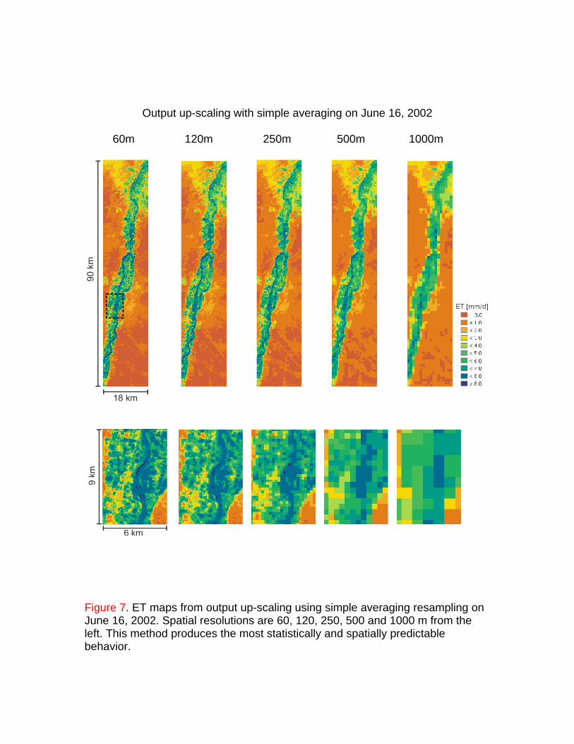
Output up-scaling with simple averaging on June 16, 2002 60m 120m 250m 500m 1000m
Figure 7. ET maps from output up-scaling using simple averaging resampling on June 16, 2002. Spatial resolutions are 60, 120, 250, 500 and 1000 m from the left. This method produces the most statistically and spatially predictable behavior.
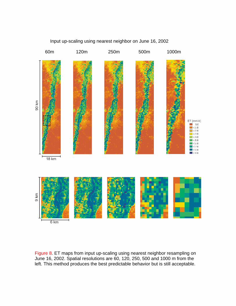
Input up-scaling using nearest neighbor on June 16, 2002 60m 120m 250m 500m 1000m
Figure 8. ET maps from input up-scaling using nearest neighbor resampling on June 16, 2002. Spatial resolutions are 60, 120, 250, 500 and 1000 m from the left. This method produces the best predictable behavior but is still acceptable.
Output up-scaling with simple averaging on June 16, 2002 60m 120m 250m 500m 1000m
0 5 10 15 20ET (mm/d)
0
4
8
12
16
20
Freq
uenc
y (%
)
↑51.4%
0 5 10 15 20ET (mm/d)
0
4
8
12
16
20
Freq
uenc
y (%
)
↑51.1%
0 5 10 15 20ET (mm/d)
0
4
8
12
16
20
Freq
uenc
y (%
)
↑50.8%
0 5 10 15 20ET (mm/d)
0
4
8
12
16
20
Freq
uenc
y (%
)
↑50.1%
0 5 10 15 20ET (mm/d)
0
4
8
12
16
20
Freq
uenc
y (%
)
↑48.0%
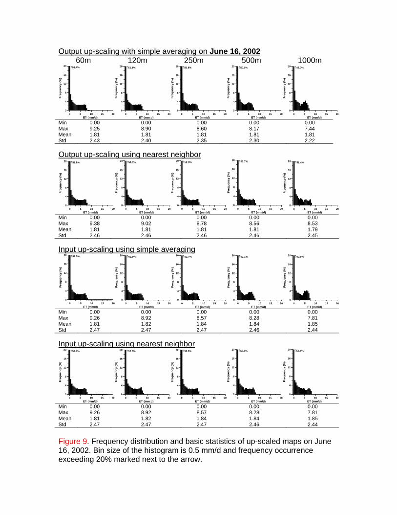
Min 0.00 0.00 0.00 0.00 0.00 Max 9.25 8.90 8.60 8.17 7.44 Mean 1.81 1.81 1.81 1.81 1.81 Std 2.43 2.40 2.35 2.30 2.22 Output up-scaling using nearest neighbor
0 5 10 15 20ET (mm/d)
0
4
8
12
16
20
Freq
uenc
y (%
)
↑51.8%
0 5 10 15 20ET (mm/d)
0
4
8
12
16
20
Freq
uenc
y (%
)
↑51.9%
0 5 10 15 20ET (mm/d)
0
4
8
12
16
20
Freq
uenc
y (%
)
↑52.0%
0 5 10 15 20ET (mm/d)
0
4
8
12
16
20
Freq
uenc
y (%
)
↑51.7%
0 5 10 15 20ET (mm/d)
0
4
8
12
16
20
Freq
uenc
y (%
)
↑51.4%
Min 0.00 0.00 0.00 0.00 0.00 Max 9.38 9.02 8.78 8.56 8.53 Mean 1.81 1.81 1.81 1.81 1.79 Std 2.46 2.46 2.46 2.46 2.45 Input up-scaling using simple averaging
0 5 10 15 20ET (mm/d)
0
4
8
12
16
20
Freq
uenc
y (%
)
↑52.5%
0 5 10 15 20ET (mm/d)
0
4
8
12
16
20
Freq
uenc
y (%
)
↑52.6%
0 5 10 15 20ET (mm/d)
0
4
8
12
16
20
Freq
uenc
y (%
)
↑52.7%
0 5 10 15 20ET (mm/d)
0
4
8
12
16
20
Freq
uenc
y (%
)
↑52.1%
0 5 10 15 20ET (mm/d)
0
4
8
12
16
20
Freq
uenc
y (%
)
↑50.9%
Min 0.00 0.00 0.00 0.00 0.00 Max 9.26 8.92 8.57 8.28 7.81 Mean 1.81 1.82 1.84 1.84 1.85 Std 2.47 2.47 2.47 2.46 2.44 Input up-scaling using nearest neighbor
0 5 10 15 20ET (mm/d)
0
4
8
12
16
20
Freq
uenc
y (%
)
↑52.4%
0 5 10 15 20ET (mm/d)
0
4
8
12
16
20
Freq
uenc
y (%
)
↑52.6%
0 5 10 15 20ET (mm/d)
0
4
8
12
16
20
Freq
uenc
y (%
)
↑52.3%
0 5 10 15 20ET (mm/d)
0
4
8
12
16
20
Freq
uenc
y (%
)
↑52.4%
0 5 10 15 20ET (mm/d)
0
4
8
12
16
20
Freq
uenc
y (%
)
↑52.4%
Min 0.00 0.00 0.00 0.00 0.00 Max 9.26 8.92 8.57 8.28 7.81 Mean 1.81 1.82 1.84 1.84 1.85 Std 2.47 2.47 2.47 2.46 2.44
Figure 9. Frequency distribution and basic statistics of up-scaled maps on June 16, 2002. Bin size of the histogram is 0.5 mm/d and frequency occurrence exceeding 20% marked next to the arrow.

Output up-scaling using simple averaging on September 14, 2000 60m 120m 250m 500m 1000m
0 5 10 15 20ET (mm/d)
0
4
8
12
16
20
Freq
uenc
y (%
)
↑65.2%
0 5 10 15 20ET (mm/d)
0
4
8
12
16
20
Freq
uenc
y (%
)
↑64.7%
0 5 10 15 20ET (mm/d)
0
4
8
12
16
20
Freq
uenc
y (%
)
↑64.6%
0 5 10 15 20ET (mm/d)
0
4
8
12
16
20
Freq
uenc
y (%
)
↑63.7%
0 5 10 15 20ET (mm/d)
0
4
8
12
16
20
Freq
uenc
y (%
)
↑62.2%
Min 0.00 0.00 0.00 0.00 0.00 Max 6.43 6.29 6.21 6.05 5.78 Mean 1.10 1.10 1.10 1.10 1.10 Std 1.76 1.74 1.71 1.66 1.60 Output up-scaling using nearest neighbor
0 5 10 15 20ET (mm/d)
0
4
8
12
16
20
Freq
uenc
y (%
)
↑65.6%
0 5 10 15 20ET (mm/d)
0
4
8
12
16
20
Freq
uenc
y (%
)
↑65.5%
0 5 10 15 20ET (mm/d)
0
4
8
12
16
20
Freq
uenc
y (%
)
↑65.6%
0 5 10 15 20ET (mm/d)
0
4
8
12
16
20
Freq
uenc
y (%
)
↑65.6%
0 5 10 15 20ET (mm/d)
0
4
8
12
16
20
Freq
uenc
y (%
)
↑65.2%
Min 0.00 0.00 0.00 0.00 0.00 Max 7.10 6.61 6.48 6.40 6.40 Mean 1.10 1.10 1.10 1.10 1.08 Std 1.78 1.78 1.78 1.78 1.75
Input up-scaling using simple averaging
0 5 10 15 20ET (mm/d)
0
4
8
12
16
20
Freq
uenc
y (%
)
↑65.7%
0 5 10 15 20ET (mm/d)
0
4
8
12
16
20
Freq
uenc
y (%
)
↑65.6%
0 5 10 15 20ET (mm/d)
0
4
8
12
16
20
Freq
uenc
y (%
)
↑65.4%
0 5 10 15 20ET (mm/d)
0
4
8
12
16
20
Freq
uenc
y (%
)
↑65.2%
0 5 10 15 20ET (mm/d)
0
4
8
12
16
20
Freq
uenc
y (%
)
↑64.4%
Min 0.00 0.00 0.00 0.00 0.00 Max 6.40 6.35 6.27 6.19 5.99 Mean 1.10 1.10 1.11 1.11 1.12 Std 1.78 1.77 1.76 1.75 1.71 Input up-scaling using nearest neighbor
0 5 10 15 20ET (mm/d)
0
4
8
12
16
20
Freq
uenc
y (%
)
↑65.6%
0 5 10 15 20ET (mm/d)
0
4
8
12
16
20
Freq
uenc
y (%
)
↑65.9%
0 5 10 15 20ET (mm/d)
0
4
8
12
16
20
Freq
uenc
y (%
)
↑65.7%
0 5 10 15 20ET (mm/d)
0
4
8
12
16
20
Freq
uenc
y (%
)
↑65.7%
0 5 10 15 20ET (mm/d)
0
4
8
12
16
20
Freq
uenc
y (%
)
↑65.7%
Min 0.00 0.00 0.00 0.00 0.00 Max 6.75 6.44 6.43 6.42 6.42 Mean 1.10 1.10 1.09 1.09 1.07 Std 1.78 1.78 1.78 1.78 1.75
Figure 10. Frequency distribution and basic statistics of up-scaled maps on September 14, 2000. Bin size of the histogram is 0.5 mm/d and frequency occurrence exceeding 20% marked next to the arrow.
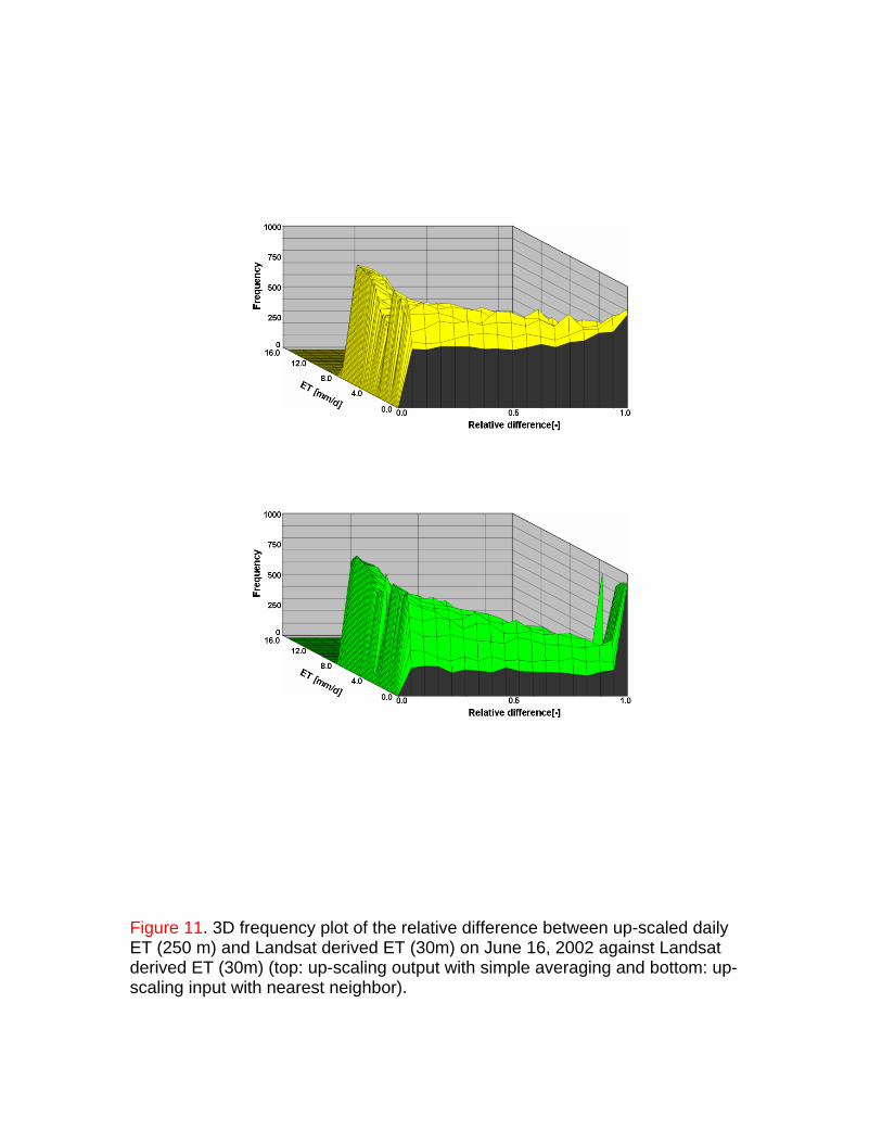
Figure 11. 3D frequency plot of the relative difference between up-scaled daily ET (250 m) and Landsat derived ET (30m) on June 16, 2002 against Landsat derived ET (30m) (top: up-scaling output with simple averaging and bottom: up-scaling input with nearest neighbor).

120 x 120 m2 pixel resolution Upscaling1 – Upscaling2 Upscaling1 – Upscaling3 Upscaling1 – Upscaling4
0 20 40 60 80 100Relative difference in ET (%)
0
5
10
15
20
25
30
Freq
uenc
y (%
)
43.4%
= 20.0= 22.3
0 20 40 60 80 100Relative difference in ET (%)
0
5
10
15
20
25
30
Freq
uenc
y (%
)
77.1%
= 7.7= 10.7
0 20 40 60 80 100Relative difference in ET (%)
0
5
10
15
20
25
30
Freq
uenc
y (%
)
50.3%
= 16.7= 19.4
1000 x 1000 m2 pixel resolution
Upscaling1 – Upscaling2 Upscaling1 – Upscaling3 Upscaling1 – Upscaling4
0 20 40 60 80 100Relative difference in ET (%)
0
5
10
15
20
25
30
Freq
uenc
y (%
)
= 41.6= 32.0
0 20 40 60 80 100Relative difference in ET (%)
0
5
10
15
20
25
30
Freq
uenc
y (%
)
69.6%
= 9.5= 8.8
0 20 40 60 80 100Relative difference in ET (%)
0
5
10
15
20
25
30
Freq
uenc
y (%
)
= 42.1= 32.3
Figure 12. Frequency of the relative difference among up-scaling schemes.