3 2013 Ahmad Erani Yustika, Susilo, Ghozali Maskie Local Government Expenditure, Economic Growth and Income Inequality in South Sulawesi Province 61-73 Journal of Applied Economics

1

VOL.1, ISSUE 3 – OCTOBER, 2013

2

Journal of Applied Economics and Business

VOL. 3, ISSUE 2 – JUNE, 2015

The Journal of Applied Economics and Business (JAEB – ISSN: 1857-8721) is an international

peer-reviewed, open-access academic journal that publishes original research articles. It

provides a forum for knowledge dissemination on broad spectrum of issues related to applied

economics and business. The journal pays particular attention on contributions of high-quality

and empirically oriented manuscripts supported by various quantitative and qualitative

research methodologies. Among theoretical and applicative contributions, it favors those

relevant to a broad international audience. Purely descriptive manuscripts, which do not

contribute to journal’s aims and objectives are not considered suitable.

JAEB provides a space for academics, researchers and professionals to share latest ideas. It

fosters exchange of attitudes and approaches towards range of important economic and

business topics. Articles published in the journal are clearly relevant to applied economics and

business theory and practice and identify both a compelling practical issue and a strong

theoretical framework for addressing it.

The journal provides immediate open-access to its content on the principle that makes

research freely available to public thus supporting global exchange of knowledge.

JAEB is abstracted and indexed in: DOAJ, EZB, ZDB, Open J-Gate, Google Scholar,

JournalITOCs, New Jour and UlrichsWeb.

Publisher

Education and Novel Technology Research Association

Web: www.aebjournal.org

E-mail: [email protected]

[email protected]

[email protected]

3

Editor-in-Chief

Noga Collins-Kreiner, Department of Geography and Environmental Studies, Center

for Tourism, Pilgrimage & Recreation Research, University of Haifa, Israel

Editorial board

Alexandr M. Karminsky, Faculty of Economics, Higher School of Economics, Russia

Anand Bethapudi, National Institute of Tourism and Hospitality Management, India

Bruno S. Sergi, Department of Economics, Statistics and Geopolitical Analysis of

Territories, University of Mesina, Italy

Dimitar Eftimoski, Department of Economics, Faculty of Administration and

Information Systems Management, St. Kliment Ohridski University, Macedonia

Evangelos Christou, Department of Tourism Management, Alexander Technological

Institute of Thessaloniki, Greece

Irena Ateljevic, Cultural Geography Landscape Center, Wageningen University,

Netherlands

Irena Nančovska Šerbec, Department of mathematics and computing, Faculty of

education, University of Ljubljana, Slovenia

Iskra Christova-Balkanska, Economic Research Institute, Bulgarian Academy of

Sciences, Bulgaria

Joanna Hernik, Faculty of Economics, West Pomeranian University of Technology,

Szczecin, Poland

Karsten Staehr, Tallin School of Economics and Business Administration, Tallin

University of Technology, Estonia

Ksenija Vodeb, Department of Sustainable Tourism Destination, Faculty of Tourism

Studies - TURISTICA, University of Primorska, Slovenia

Kaye Chon, School of Hotel and Tourism Management, the Hong Kong Polytechnic

University, China

Pèter Kovács, Faculty of Economics and Business Administration, University of

Szeged, Hungary

Ramona Rupeika-Apoga, Faculty of Economics and Management, University of

Latvia, Latvia

Renata Tomljenović, Institute for Tourism, Zagreb, Croatia

Valentin Munteanu, Faculty of Economics and Business administration, West

University of Timisoara, Romania

http://www.aebjournal.org/editorialteam.php
















4

Content

Andromahi Kufo

Albanian Banking System: Risk Behavior and Capital Requirements 5-16

Allen L. Webster

Testing the Relationship between Economic Freedom

and Income Inequality in the USA 17-38

Lavdrim Sahitaj, Olta Allmuça, Alba Allmuça Ramallari

Human Resources in the International Organization’s Context 39-48

Isaac Mokono Abuga, Michael Manyange Nyasimi

Effectiveness of Mobile Banking Services in

Selected Commercial Banks in Rwanda 49-60

Sabir, Ahmad Erani Yustika, Susilo, Ghozali Maskie

Local Government Expenditure, Economic Growth and

Income Inequality in South Sulawesi Province 61-73


5

ALBANIAN BANKING SYSTEM: RISK

BEHAVIOR AND CAPITAL

REQUIREMENTS

Andromahi Kufo

Faculty of Economics, University of New York, Tirana, Albania

[email protected]

Abstract

With almost 20 years history, the Albanian banking system struggles from one side to ensure the

economy safety and soundness and from the other side to comply with international requirements such

as Basel II. In this crossroad, we attempt to investigate the regulator’s effect on the monitoring and

supervising the banking system and the banks behavior towards these requirements. This article finds

a significant positive and simultaneous relationship between risk and capital for the Albanian banking

sector which relies on previous theoretical and empirical approaches.

Key words:

Risk behavior; Capital requirements; Banking system; Albania.

INTRODUCTION

Albanian banking system roots date just 20 years before in 1998, when the first private

banks started their activity in the local market economy, which had some years

changed from communism into the capitalistic system. The private banks started their

activity in a primitive market place, where the concepts of financial intermediation

and banking were almost unknown. Mostly foreign bank groups from Greece and

Italy started to open their branches in order to fulfill the foreign business’s needs, until

the privatization of the savings banks and commercial banks (two of the most

powerful state banks) from the well-known Austrian and Turkish groups created

leaders in the banking market place. Local banks started as well to perform activities

and here we are in 2015 with 16 banks working in Albania, under the regulation of the

central Bank of Albania.

It is understandable that such a flourish in the banking system would require at least

regulation and monitoring from the authorities, in order to keep the system and the

Andromahi Kufo

Albanian Banking System: Risk Behavior and Capital Requirements

6 JOURNAL OF APPLIED ECONOMICS AND BUSINESS, VOL. 3, ISSUE 2 -JUNE, 2015, PP. 5-16

economy safe. Bank of Albania had to deal with a lot of circumstances where fast and

relevant regulation had to be prepared and rule the banks so as to keep control and

ensure soundness. One of the oldest regulations of the Bank of Albania was that

referring to the capital requirement in 1999. Even though the urge to comply with

international requirements of Basel, not until the end of 2014, this regulation has been

reviewed and adopted some of the standards of Basel II. The challenge of the local

banking system in adopting these requirements is part of another research paper. This

paper will mainly concentrate on the banks behavior towards risk trying to identify

the relationship between risk and capital.

Using a data set of six years from the last quarter of 2008 until the last quarter of 2014,

this research proves the positive relationship between risk and capital, as defined also

in previous literature from a theoretical and practical prospective. The two stages least

square model adopted from Shrives and Dahl (1992) was used in this data to prove

that the behavior of Albanian banking sector towards risk is affected positively from

the requirements of capital that the authorities apply and on the other hand also the

capital changes are affected from the risk behavior that banks decide to follow. This

gives a strong ally on the authorities, which are actually doing a good job in the

monitoring and supervision of the banking system. It also supports the fact that the

regulator reacts promptly and seriously on the crisis matters, as well as on the

international developments of the banking system, even though the local system is

actually “protected” in terms of not being exposed to external crisis factors.

The paper follows with a review on different models that have tried to present the

relationship between risk and capital. It follows with the explanation of data and

methodology. Finally results and conclusions complete this attempt. It is of big

interest to review the behavior of banks in the following years, since more

requirements with the international standards will affect their capital requirements

and their activity.

LITERATURE REVIEW

As stated in earlier and recent literature the regulation of capital in banks is very

important. The reasons behind this importance rely upon certain arguments: the

systemic risk argument and the depositors’ representative argument. The capital

requirements are proved to be necessary in terms of controlling the risk appetite of the

banks, the banks solvency and the amount of deposits. The regulators have to find the

proper optimal solution between the risk of default and the deposits and they have to

represent the depositors’ inability to monitor the banks.

The literature has presented many theories regarding the way that capital and risk are

affecting each other, using different financial models. These financial models should

be discussed regarding the economic rationale of the relationship capital –risk,


7

whether this relationship has a positive or a negative sign and how this relationship

is influenced from the changes in regulatory framework.

The option pricing model adopted by earlier literature (Merton, 1977; Black et al, 1978;

Kareken & Wallace, 1978; Dothan & Williams, 1980; Marcus & Shaked, 1984; Diamond

& Dybvig, 1986; Benston et al, 1986) introduces the idea that the maximization of the

stockholders’ equity value implies maximization of the option value of the deposit

insurance increasing leverage and asset risk. This means that banks can increase their

deposit liability without paying for a default risk premium and the marginal effect

from this action increases as asset risk increases. At the same time, the marginal benefit

of the increasing asset risk increases as leverage increases (equity capital decreases).

Although the increases in leverage and risk are proved to be profitable, they imply

certain costs that do not permit an infinite increase. According to the banks’ behavior

dominance towards increasing insurance deposits or increasing risk appetite then we

would observe a negative relationship between capital and risk in the first case and a

positive relationship capital and risk in the second case.

Theories that imply a positive relationship between capital and risk due to a margin

in the combination of leverage and risk rely on the regulatory costs (Buser at al, 1981),

effects of minimum capital requirements (Merton, 1972; Kahane, 1977; Koehn &

Santomero, 1980; Kim & Santomero, 1988), bankruptcy cost avoidance (Orgler &

Taggart, 1983) and managerial risk aversion (Saunders at al, 1990).

Shrieves and Dahl (1991) have explained and reviewed the theory and through their

research they developed a model trying to explain and estimate the changes in the

relationship between capital and risk. Their results show that capital and risk are

simultaneously related and a bank tends to increase its asset risk in case of an increase

in capital imposed by regulators. This is more obvious in banks that have low level of

capital. The results are consistent with the leverage and risk related cost avoidance

and managerial risk aversion theories of capital structure and risk-taking behavior on

commercial banks. So the effectiveness of the capital standards is subject to the

reflection of true risk exposure of the banks.

Calem and Rob (1996) discuss the impact of the capital-based regulation on the bank

risk-taking behavior through a dynamic portfolio model using empirical data from

the US market from 1984-1993 with the aim of defining the capital regulations effects

on the risk of the institutions. Their results suggest of a relationship between risk and

capital, where increased capital requirements induce in greater risk-taking of well-

capitalized banks, whereas they also induce in increased risk of under-capitalized

banks, if the regulations are not stringent enough, consisting in some unintended

results.

Andromahi Kufo



Ediz et al, (1998) have studied the implication of capital requirements in the UK banks’

behavior and they prove that U.K. banks behavior is affected from capital requirement

over and above their own capital targets. In case an increase in the capital is required,

this is assured from the market other than from increasing assets.

Blum (1999) has introduced a new model for capital and risk taking into consideration

the dynamic banking environment. The main point of his study evaluates that under

binding regulatory requirements on capital an additional unit of equity tomorrow is

more valuable to the bank, so the only possibility to increase the equity tomorrow, is

to increase the risk today. This means that more stringent capital requirements today

will increase the bank’s risk.

In the research work of Rime (2000) through empirical evidence from Swiss banks

regarding capital requirements and bank’s behavior using a modified model from

Shrieves and Dahl (1991) it is found that banks close to regulatory minimum tend to

increase their ratio of capital to risk-weighted assets. Moreover the regulatory impact

is evident to the ratio of capital to asset, but not to the bank’s risk taking. Also he finds

a significant relation between changes in risk and changes in the ratio of capital to total

assets, but not a significant relation between changes in risk and changes in the ratio

of capital to risk-weighted assets.

Lindquist (2003) uses an empirical model to measure the effect of the buffer capital in

relation with credit risk in Norway bank. He divides the data into commercial and

savings banks for a period from 1995 until 2001 and tests the issues of buffer capital

being affected from credit risk, it acts as an insurance for not falling below minimum

capital requirements, it is used as a signal i.e. competition parameter, it depends on

economic growth and finally if as a measurement of supervision it really matters for

banks. The results for capital and credit risk show a negative relationship for saving

banks measured by the variance of profits of previous years considered as a “broad

risk measure”. This actually counter-argues previous results of literature, but it is

explained by the author as an attempt from banks to act in various ways towards risk.

Cuoco and Liu (2005) come with a different fully dynamic optimal portfolio model to

assess the relationship between capital requirements and VaR as determined by the

Internal Model Approach introduced in Basel II. The value at risk measure VaR which

defines the maximum losses of financial institutions varies according to the capital

requirements that the regulator imposes to the banks and is adjusted by re-balancing

the bank’s portfolio. This specific “re-balancing trading strategy” followed by banks

implies that VaR may be over or underreported according to the risk appetite banks

select for the specific time period. In general self-reported VaR defined by IMA

suggest that more stringent capital requirements induce a portfolio selection with

higher return assets, which also have higher risks in relation to the regulation weights

suggesting also a higher probability of default for those institutions.


9

Godlewksi (2006) investigated the effects of the regulatory framework in the banks

behavior in emerging markets and proved a significant relationship between them

that could even degenerate into excessive risk taking and increase in the banks’

probability of default. He notes though that the results need further investigation that

would include internal corporate governance factor and external ones concerning

market discipline.

A positive relationship between risk and capital has been also found by Altunbas et

al, (2007), when they examined the European banks on the behavior on the

relationship between the capital, risk and efficiency. Through empirical evidence from

1992 until 2000 on a sample of European banks the authors have not found a positive

relationship between risk and efficiency as proved empirical studies in the US, but

they have introduced a positive relationship between risk and capital in commercial

and savings banks and a negative one in co-operating banks.

A similar study on 263 Japanese co-operative banks regarding the relationship

between risk, capital and efficiency for the period 2003-2006 was performed by

Deelchand and Padgett (2009). Adopting the simultaneous equations of Shrieves and

Dahl etc. regarding capital, risk and efficiency the empirical data show an important

negative relationship between risk and capital as well as inefficient banks maintaining

more capital, which actually support the moral-hazard theory. The authors suggest

that more it is needed a closer monitoring from the supervisory authorities regarding

loan expansions, bank efficiency and capital adequacy requirements for Japanese

banks.

All the above literature represents the relationship between capital and risk under

different conditions, taking into account various factors and explaining based on

theories the impact of changes in the capital adequacy requirements to the bank’s

behavior towards risk.

As per Albanian banking sector, it lacks such studies in terms of identifying the banks’

behavior and the regulator’s influence. This is what we try to perform in this study:

discuss the relationship between capital requirements imposed by the Bank of Albania

and the behavior of Albanian banking sector towards risk for a six-years period

2008:Q4-2014:Q4.

HYPOTHESES, MODEL AND DATA

Based on the above empirical researches we state below the basic hypotheses tested in

this research:

Hypothesis 0: In a regulated environment capital and risk of banks are not

interrelated and affected by each other.

Andromahi Kufo



Hypothesis 1: In a regulated environment, where capital requirements increase, the

risk of the bank decreases due to the dominance of the deposit insurance subsidy,

which defines the marginal benefits and costs of asset risk and leverage. This

means that the capital will have a negative relationship with the risk.

Hypothesis 2: In a regulated environment where capital requirements increase,

compensation on the risk weighted assets of the bank will take place so as to

increase the ratio of capital to total assets in order to maintain their default

probability at an accepted level. This means that the capital will have a positive

relationship with the risk.

Hypothesis 4: In a regulated environment capital and risk are simultaneously

related with each other.

Model specifications

We are based on the simultaneous model initially described by Shrives and Dahl

(1991) and consequently by Rime (2001), as well as other authors described above. In

this equation the capital and risk are simultaneously affecting each other, which may

include as we mentioned above a negative or appositive relationship according to

different approaches.

The basic equations are presented below and carried out by two stage least squares

model (TSLS):

ΔCAP j,t = a0 +a1REGj,t-1 + a2ROAj,t +a3SIZE + a4 ΔRISK j,t - a5 CAPj, t-1 + εj,t ;

ΔRISK j,t = a0 +a1REGj,t-1 + a2LLossj,t +a3SIZE + a4 ΔCAP j,t - a5 RISKj, t-1 + νj,t ;

Due to the fact that ΔCAP j,t and ΔRISK j,t are simultaneously affecting each other, we

had to run the two stages least square model, where instrumental variables for a

regression at step one are defined and the predicted values saved from first step are

then used for the second regression at step two. Specifically, at the first step, we

regressed the independent variables needing instrumental variables on the

instrumental variables and other independent variables not needing instrumental

variables. Then, we saved the predicted values to form some new variables. At the

second step, we regressed the dependent variable on these new variables and other

independent variables not needing instrumental variables. The whole process was

performed in SPSS, where for each equation we selected the dependent variable then

selected the instrumental variables and the other independent variables not needing

instrumental variables and finally defined all independent variables (not

instrumental) as explanatory to the model.

The variables include the following:

ΔCAP j,t represents the change in capital. Considering the fact that banks may not be

able to adjust their desired capital ratio instantly, the variable is defined as the

difference between the capital of two consecutive quarters:


11

ΔCAP j,t = a(CAP j,t - CAP j,t-1) + E j,t

This is defined as a ratio of equity over total assets, where equity includes common

stocks, preferred stocks, capital surplus, undivided profits, capital reserves and

foreign currency translation adjustments. It is the dependent variable of the first

equation. We actually expect that capital will be positively affected by the risk banks

undertake.

ΔRISK j,t represents the change in risk level of the bank. Again considering the fact

that banks may not be able to adjust their desired risk ratio instantly, the variable is

defined as the difference between the risk of two consecutive quarters:

ΔRISK j,t = b (RISK j,t - RISK j,t-1) + Sj,t

Risk is defined as the ratio of risk –weighted assets over total assets. Risk-weighted

assets are defined according to the Bank of Albania regulation by imposing different

weights to certain categories. Risk is the dependent variable of the second equation

and we expect a positive relationship between risk and capital.

REGj,t-1 represents the binary variable for regulation changes affecting the bank’s

capital and risk. This is a dummy variable, which actually takes the value 0 to display

no changes in the regulatory framework and 1 otherwise. Even though the Bank of

Albania has not made any changes in the regulatory framework, it has imposed

different capital requirements for Greek banks operating in Albania in the last quarter

of 2011. This due to the increased risk of the Greek banking sector and the collapse in

2011 and the high probability of default these banks actually involved. So instead of a

capital requirement of 12% for the whole sector, Bank of Albania imposed a 15%

capital requirement for these banks. This actually leaded into an increased necessity

for capital from the Greek banks. We expect to have a positive relation between capital

and regulation and a negative relationship between risk and regulation.

ROAj,t represents the return on assets as a measure of profitability of the bank. It is

included in the capital equation and it is expected to have a positive relationship with

capital. Well-capitalized banks may use their profits to increase capital, rather than

requiring additional capital from their mother companies (this because issuing capital

in Albanian market is not applicable).

LLossj,t represents the current loan losses and is included in the risk equation. It is

measured as a ratio of the difference in the provisions over two consecutive periods

over total assets. New provisions are actually considered to represent the current loan

losses of the bank, which decrease the risk-weighted assets and as such affect the ratio

of risk-weighted assets to total assets. Consequently we expect a positive relation

between the loan losses and the risk of the bank.

Andromahi Kufo



SIZE is calculated as the natural logarithm of total assets as a measure to be included

in both capital and risk equation. This is based on the assumption that size may affect

target risk and capital because of its relation with diversification, investment

opportunities and access to equity capital.

Under the models represented above the bank independently chooses capital and risk,

as such both variables are included as independent variables to each of the equations.

Data

The sample used in this research includes the 16 banks of the local banking sector, for

a period of 2008Q4 until 2014Q4. The collection includes the basic reporting of banks

to the Bank of Albania according to local regulation on a quarterly basis. During this

period there were in total 352 observations for the first equation and 287 observations

for the second equation.

RESULTS AND DISCUSSION

From the results of the simultaneous equations run in the two stages least square

regression model, seem important; in the first equation the independent variable is

explained at a level of 50% by the dependent variables, while in the first equation the

independent variable is explained at a level of 30% as detected from the multiple R.

The R-square for the first equation makes the model more explanatory at a level of

25%. The reliability of the models though is significant according to the F-statistics and

its level of confidence 0.00 presented in the appendix, showing a linear relationship

between capital and risk simultaneously.

The first equation’s results show that the capital is dependent on the risk level that

banks undertake, having a positive relationship and t-value at a significance level of

less than 0.05, accepting our third and fourth hypothesis at the same level of

confidence. Capital and risk are positively related to each other for the Albanian

banking sector based on the theory of keeping its default probability at the same level.

As per other explanatory variables, regulation and return on assets have a positive

relationship in explaining capital changes, though not proved as significant from the

model. On the other hand size is negatively affecting capital, though without a

significant affection. None of the variables is highly correlated on a positive or

negative way with the other.

The second equation shows that risk is dependent on the capital level that a bank

retains. Their relationship once again is positive and the t-value at a significance level

of less than 0.05, accepting our third and fourth hypothesis at the same level of

confidence. Risk and capital are positively related to each other for the Albanian

banking based on the theory of keeping its default probability at the same level.

Regulation and size are negatively affecting the risk, although their coefficients do not

show any high significance. We have noted though that the explanatory variable of


13

losses has a significant positive relationship with the risk. We have defined this

variable as the difference of provisions of two consecutive years over total assets of

the bank. As we expected this relationship is actually proved significant through the

equation. This variable is also highly correlated with the change in capital at a

correlation coefficient level of 0.89, as well as with the risk at a correlation coefficient

level of 0.63, identifying the high importance effect and direct relationship that the

variable has with both capital and risk. This is also due to the method of defining the

regulatory capital and risk weighted assets according to the current regulation of the

Bank of Albania.

The actual model of this research proved the simultaneous relationship between risk

and capital and justified the acceptance of hypothesis 4 and the rejection of hypothesis

0. The relationship between risk and capital is simultaneously proved as significant

and positive, as such accepting hypothesis 3 and rejecting hypothesis 2.

The size effects even though negatively related with both risk and capital are proven

not to be significant in the bank’s behavior towards risk; this means that in the current

market banks are well-capitalized and just by being a larger bank does not justify

excessive risk. Bank’s efficiency in terms of profitability (ROA) does not affect the

capital that it retains. This is due initially to the fact that the regulatory capital is

defined according to specific weights and not using other methods implied in Basel II.

The provisions as a measure of banks’ losses are actually positively and significantly

related with the risk, showing once again how application of the provisions regulation

affects the regulatory capital and the risk simultaneously. The results of this specific

measurement though are controversial from the hypotheses we made for it.

Regulation on the other hand affects neither the capital nor the risk of the bank,

although it has a positive relationship with them. Even though there has been only a

change in the requirement of the regulatory capital in the last quarter of 2011 and only

for Greek banks, this did not affect our model. That actually guides to the conclusion

of having a well-capitalized banks, which can afford any regulatory pressure by not

actually affecting their capital and their behavior towards risk.

In general we can refer that our results were in consistency with two of our main

hypotheses at a confidence level higher than 99%. All results appear in the appendix.

CONCLUSION

Risk and capital have a positive significant and simultaneous relationship between

them for the Albanian banking system. Neither the profitability nor the size of a bank

affects its’ regulatory capital suggesting strong monitoring from the regulator. The

system is well supervised in such way that no undercapitalized banks are present in

the sector. The efficiency of the regulator is considered high, but also the compliance

Andromahi Kufo



of the active in the marketplace banks is considered on a high level. It is of major

interest to further research on the banks behavior towards risk in the following years,

when banks will have to comply with the new regulation, closed to the Basel

requirements.

REFERENCES

Altunbas, Y., Carbo, S., Gardener, E. P. M. & Molineux, P. (2007). Examining the

relationship between capital, risk and efficiency in European banking. European

Financial Management, 13(1), 49-70.

Bank of Albania. 2009-2014. Annual reports.

Benston, G. J., Eisenbeis, R. A., Horvitz, P. M., Kane, E. J. & Kaufman, G. G. (1986).

Perspectives on safe & sound banking. MIT Press, Cambridge, MA.

Black, F., Miller, M. H. & Posner, R. A. (1978). An approach to the regulation of bank

holding companies. Journal of Business 51, 379-412.

Blum, J. (1999). Do capital adequacy requirements reduce risks in banking?. Journal of

Banking and Finance, 23(5), 755-771.

Buser, S., Chen, A. & Kane, E. (1981). Federal deposit insurance, regulatory policy, and

optimal bank capital. Journal of Finance, 36, 51-60.

Calem, J. & Rob, R. (1996). The impact of capital-based regulation on bank risk taking.

Federal Reserve publications.

Cuoco, D. & Liu, H. (2006). An analysis of VaR-based capital requirements. Journal of

Financial Intermediation, 15, 362-394.

Deelchand, T. & C. Padgett. (2009). The relationship between risk, capital and

efficiency: evidence from Japanese cooperative banks, ICMA Centre Discussion Paper

in Finance, DP2009-12.

Diamond, D. W. & Dybvig, P.H. (1986). Banking theory, deposit insurance and bank

regulation. Journal of Business, 59, 55-67.

Dothan, U. & Williams, J. (1980). Banks, bankruptcy and public regulation. Journal of

Banking and Finance, 4, 655-688.

Ediz, T., Michael, I. & Perraudin, W. (1998). The impact of capital requirements on UK

bank behavior. FRBNY Economic Policy Review, 4(3), 15-22.

Godlewski, C. J. (2006). Regulatory and institutional determinants of credit risk taking

and a bank's default in emerging market economies: a two-step approach. Journal of

Emerging Market Finance, 5(2), 183-206.


15

Kahane, Y. (1977). Capital adequacy and the regulation of financial intermediaries.

Journal of Banking and Finance 1, 207-217.

Kareken, J. H. & Wallace, N. (1978). Deposit insurance and bank regulation: A partial

equilibrium exposition. Journal of Business 51, 413-438.

Kim, D. & Santomero, A. M. (1988). Risk in banking and capital regulation. Journal of

Finance, 43, 1219-1233.

Koehn, M. & Santomero, A. M. (1980). Regulation of bank capital and portfolio risk.

Journal of Finance, 35, 1235-1250.

Lindquist, K. (2003). Banks’ buffer capital: How important is risk?, Norges Bank

working papers, Department of Research.

Marcus, A. J. & Shaked, I. (1984). The valuation of FDIC deposit insurance using

option pricing estimates. Journal of Money, Credit, and Banking, 16, 446-460.

Merton, R. C. (1972). An analytic derivation of the efficient frontier. Journal of

Financial and Quantitative Analysis, 7, 1851-1872.

Merton, R. C. (1977). An analytic derivation of the cost of deposit insurance and loan

guarantees. Journal of Banking and Finance, 1, 3-11.

Orgler, Y. E. & Taggart, R. A. Jr. (1983). Implications of corporate capital structure

theory for banking institutions. Journal of Money, Credit, and Banking, 15, 212-221.

Rime, B. (2000). Capital requirements and bank behavior: empirical evidence for

Switzerland. Swiss National Bank, Banking Studies Section.

Saunders, A., Strock, E. & Travlos, N. G. (1990). Ownership structure, deregulation,

and bank risk taking. Journal of Finance, 45, 643-654.

Shrieves, R. E. & Dahl, D. (1991). The relationship between risk and capital in

commercial banks. Journal of Banking and Finance, 16(2), 439-457.

APPENDIX Two-stage Least Squares Analysis

Table 2. Model Summary

Equation 1

Multiple R .500

R Square .250

Adjusted R Square .236

Std. Error of the Estimate .009

Table 1. Model Description: MOD_5

Equation 1

ΔCAPjt Dependent

a1REGjt1 predictor & instrumental

a2ROAjt predictor & instrumental

a3SIZE predictor & instrumental

a5CAPjt1 predictor & instrumental

ΔRISKjt Predictor

a2LLossjt Instrumental

a5RISKjt1 instrumental

Andromahi Kufo



Table 5. Coefficient Correlations

a1REGjt1 a2ROAjt a3SIZE a5CAPjt1 ΔRISKjt

Equation 1 Correlations a1REGjt1 1.000 -.145 .134 -.041 .016

a2ROAjt -.145 1.000 -.184 .231 -.115

a3SIZE .134 -.184 1.000 .606 -.006

a5CAPjt1 -.041 .231 .606 1.000 .181

ΔRISKjt .016 -.115 -.006 .181 1.000

Table 10. Coefficient Correlations

ΔCAPjt a1REGjt1 a3SIZE a2LLossjt a5RISKjt1

Equation 1 Correlations ΔCAPjt 1.000 -.121 -.143 .896 .631

a1REGjt1 -.121 1.000 .119 -.096 -.088

a3SIZE -.143 .119 1.000 -.159 .442

a2LLossjt .896 -.096 -.159 1.000 .566

a5RISKjt1 .631 -.088 .442 .566 1.000

Table 3. ANOVA

Sum of

Squares df

Mean

Square F Sig.

Eq

uat

ion

1 Regression .007 5 .001 18.766 .000

Residual .022 282 .000

Total .029 287

Table 4. Coefficients

Unstandardized

Coefficients Beta t Sig.

Eq

uat

ion

1

(Constant) .000 .007 -.029 .977

a1REGjt1 .001 .002 .018 .619 .536

a2ROAjt .000 .000 .024 .713 .476

a3SIZE -3.591E-05 .001 -.003 -.065 .948

a5CAPjt1 -.006 .006 -.044 -1.030 .304

ΔRISKjt .068 .008 .660 8.315 .000

Table 6. Model Description: MOD_6

Type of Variable

Equation 1 ΔRISKjt dependent

ΔCAPjt predictor

a1REGjt1 predictor & instrumental

a3SIZE predictor & instrumental

a2LLossjt predictor & instrumental

a5RISKjt1 predictor & instrumental

a2ROAjt instrumental

a5CAPjt1 instrumental

Table 7. Model Summary

Equation 1 Multiple R .276

R Square .076

Adjusted R Square .060

Std. Error of the Estimate .223

Table 8. ANOVA

Sum of

Squares df

Mean

Square F Sig.

Eq

uat

ion

1 Regression 1.162 5 .232 4.657 .000

Residual 14.070 282 .050

Total 15.231 287

Table 9. Coefficients

Unstandardized

Coefficients Beta t Sig.

Eq

uat

ion

1

(Constant) .061 .165 .369 .713

ΔCAPjt 21.012 5.803 2.178 3.621 .000

a1REGjt1 -.021 .044 -.037 -.482 .630

a3SIZE -.007 .014 -.057 -.526 .599

a2LLossjt 7.279 3.418 .366 2.130 .034

a5RISKjt1 .022 .020 .150 1.098 .273


17

TESTING THE RELATIONSHIP

BETWEEN ECONOMIC FREEDOM AND

INCOME INEQUALITY IN THE USA

Allen L. Webster

Foster College of Business, Bradley University, Peoria, Illinois, USA

[email protected]

Abstract

The Gini coefficient is used to examine the impact of economic freedom on income inequality among

the 50 US states. The degree of economic freedom is provided by the Fraser Institute in Vancouver,

Canada. A fixed-effect model based on panel data from 2000-2013 is estimated to determine if

differences exist among the four census regions identified by the US Census Bureau. The findings

clearly suggest that those states characterized by higher levels of economic freedom exhibit greater

income equality. A Dickey-Fuller test for stationary revealed the need for first-differencing and a

Granger-causality test concluded that uni-directional causality existed between income distribution

and economic liberty.

Key words

Gini Coefficient; Economic Freedom; Income Distribution; Fixed-Effects Models; Granger Causality.

INTRODUCTION

Considerable attention has been devoted to the trend in income inequality in the

United States over the past several years. This concern has become a particularly

critical issue among economists, business leaders and even the concerned citizenry.

Political figures attempting to draw attention to their social conscience have also

attached themselves to this pressing socio-economic dilemma.

In his December 4, 2013 speech before the Center for American Progress, President

Obama praised the New Deal and the War on Poverty for building “the largest middle

class the world has ever known,” but regretfully alluded to the “dangerous and

growing inequality and lack of upward mobility that has jeopardized middle-class

America’s basic bargain – that if you work hard, you have a chance to get ahead”.

Although somewhat positive in nature, his address carried the message that progress

has stalled and income disparities have widened perceptively. Much of the available

Allen L. Webster Testing the Relationship between Economic Freedom and Income Inequality in the USA


data seem to support the President's contention. It is generally agreed that income

inequality has been on the rise in the United States since the late 1970s. Recent studies

have shown that income disparities began to increase in the U.S. economy in the early

1970s and continue today (Webster, 2014; Apergis, et al, 2011; Ram, 2012). Sommeiller

and Price (2014), for example, find that between 1979 and 2007, the top 1% income

earners took home over one-half (53.9%) of the total increase in US income. Over that

same period, the average income of the bottom 99% grew by only 18.9%.

This gap between the income classes has often been cited as a precursor for many

socio-economic ills ranging from poverty, impediment to economic growth, elevated

crime rates and general social disorder. Over the past several decades, after-tax

incomes for the top 1% of households grew 275%. This compares to an 18% rise of the

incomes of those in the bottom quintile. According to Piketty and Saez (2003), the top

“1%ers” took home a 95% gain in the first three years of the recovery following the

Great Recession. Furthermore, Piketty (2014) argues that the central contradiction of

capitalism is that it leads to the concentration of wealth in the hands of those who are

already rich. He denounces the evils of free markets and the inequities they produce.

Piketty (2014) is particularly loathsome of inherited wealth. He contends that it

generates slower economic growth and increases the ratio of capital to income which

further exacerbates the disparities in incomes.

A common measure of income inequality is the Gini coefficient developed by the

Italian economist and statistician Corrado Gini (1997). As an index of inequality, the

coefficient (or ratio) ranges between zero and 1.00. The lower the coefficient is, the

more equally incomes are dispersed throughout the economy. From all accounts, the

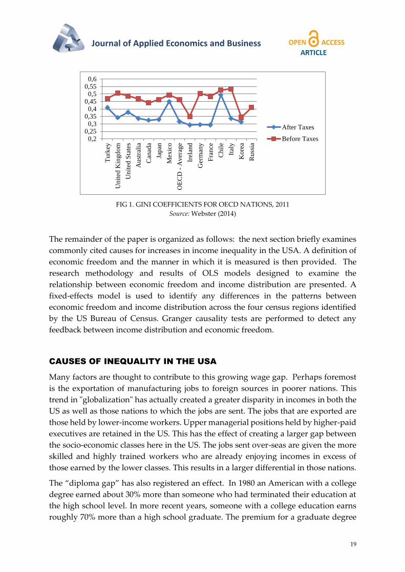
US does not compare favorably to many other nations. Figure 1 provides Gini

coefficients for some of the 34 nations that constitute the Organization for Economic

Cooperation and Development (OECD) (Webster, 2014). Russia, which is not a

member nation, is also included for comparison. The upper values represent the

coefficients before taxes and transfers while the lower values are the ratios after taxes

and transfers have reduced the degree of inequality. It can be seen that only Chile,

Turkey and Mexico report after-tax Ginis greater than the US. The after- tax Gini for

Russia is unavailable. The OECD averages of 0.316 and 0.463 are also included.

It is interesting to note the net changes in the degree of inequality after taxes and

transfers. For example, Canada’s Gini coefficient was reduced by over 0.10 through

public efforts to combat income inequality.

Clearly, France, Germany and Italy reduced their coefficients the most while Chile,

Ireland, Korea and Mexico had very little effect on the coefficients as a result of

transfers from the wealthy to the poor. The mean reduction was 0.1106 and the

median was 0.117. The less well of in Germany benefited the most as that nation’s Gini

coefficient dropped by 0.209 while that of Mexico fell the least by 0.018. The US

reduction was 0.108. The mean OECD decrease was 0.147.


19

FIG 1. GINI COEFFICIENTS FOR OECD NATIONS, 2011

Source: Webster (2014)

The remainder of the paper is organized as follows: the next section briefly examines

commonly cited causes for increases in income inequality in the USA. A definition of

economic freedom and the manner in which it is measured is then provided. The

research methodology and results of OLS models designed to examine the

relationship between economic freedom and income distribution are presented. A

fixed-effects model is used to identify any differences in the patterns between

economic freedom and income distribution across the four census regions identified

by the US Bureau of Census. Granger causality tests are performed to detect any

feedback between income distribution and economic freedom.

CAUSES OF INEQUALITY IN THE USA

Many factors are thought to contribute to this growing wage gap. Perhaps foremost

is the exportation of manufacturing jobs to foreign sources in poorer nations. This

trend in "globalization" has actually created a greater disparity in incomes in both the

US as well as those nations to which the jobs are sent. The jobs that are exported are

those held by lower-income workers. Upper managerial positions held by higher-paid

executives are retained in the US. This has the effect of creating a larger gap between

the socio-economic classes here in the US. The jobs sent over-seas are given the more

skilled and highly trained workers who are already enjoying incomes in excess of

those earned by the lower classes. This results in a larger differential in those nations.

The “diploma gap” has also registered an effect. In 1980 an American with a college

degree earned about 30% more than someone who had terminated their education at

the high school level. In more recent years, someone with a college education earns

roughly 70% more than a high school graduate. The premium for a graduate degree

0,20,25

0,30,35

0,40,45

0,50,55

0,6

Tu

rkey

Un

ited

Kin

gd

om

Un

ited

Sta

tes

Au

stra

lia

Can

ada

Jap

an

Mex

ico

OE

CD

- A

ver

age

Irel

and

Ger

man

y

Fra

nce

Chil

e

Ital

y

Ko

rea

Russ

ia

After Taxes

Before Taxes



has increased from roughly 50% in 1982 to well over 100% today in some instances

(Webster, 2014). Given the explosive rise in the cost of a college education, only those

in the more affluent classes can afford more extensive schooling. This has the effect of

widening still further any prevailing income differences.

The decline in the level of unionization across the United States has further magnified

the separation of the income classes. Evidence has shown (Western & Rosenfeld, 2011;

Card & Lemieux, 2004) that incomes are more evenly distributed in areas with higher

rates of unionization. In 1983, 20.1% of the labor force or 17.7 million workers were

union members. Today those figures stand at 11.3% and 14.5 million members. The

impact of such dynamics on the wage gap is evident when it is considered that in 2013

the median weekly earnings for union members was $950, while those who were not

union members had median weekly earnings of only $750 (US Department of Labor,

January 24, 2014). Further, as fewer union members occupy the work force the gap

must widen since the incomes of high-earning management do not depend on union

membership.

It is generally recognized that tax laws tend to favor the wealthy. Provisions that affect

stock options and capital gains permit the wealthy to shelter their incomes from the

tax man. Many argue this lessens the tax burden on the wealthy and has accelerated

the separation between the rich and the poor.

ECONOMIC FREEDOM

Although several other forces can be identified that affect income deviation, strong

indication persists that income dispersion is also influenced by the degree of economic

freedom prevailing in a political or geographical unit. Although no universally

accepted definition of economic freedom has been established, it generally refers to

the ability of economic participants to make decisions and take actions without

restraint from central forces. It is philosophically based on principles ranging from

pure laissez-faireism to that advocated by the classical libertarian. Emphasis is placed

on reliance on free markets, private property and individual choice.

Most studies rely on the index of economic freedom (EFI) developed by the Fraser

Institute in Vancouver, Canada. The Institute provides an annual cardinal measure of

the extent of economic freedom prevailing in all 50 U.S. states as well as all Canadian

providences. These data are provided in annual reports entitled the Economic Freedom

of North America. The Institute defines economic freedom as a condition in which

Individuals have economic freedom when (a) property they acquire… is

protected from physical invasion by others and (b) they are free to use, exchange

or give their property as long as their actions do not violate the identical rights

of others. Thus, an index of economic freedom should measure the extent to


21

which rightly acquired property is protected and individuals are engaged in

voluntary transactions.

The indices of economic freedom used by the Fraser Institute focus on six areas of

concern. Each area contains subcategories as shown in Table 1.

TABLE 1.THE AREAS AND COMPONENTS OF ECONOMIC FREEDOM OF NORTH AMERICA

INDEX

Area 1-Size of Government

1A-General Consumption Expenditures by Government as a Percentage of GDP

1B -Transfers and Subsidies as a Percentage of GDP1

1C-Social Security Payments as a Percentage of GDP

Area 2-Takings and Discriminatory Taxation

2A-Total Tax Revenue as a Percentage of GDP

2B-Top Marginal Income Tax Rate and the Income Threshold at Which It Applies

2C-Indirect Tax Revenues as a Percentage of GDP

2D-Sales Taxes Collected as a Percentage of GDP

Area 3-Regulation

3A-Labor Market Freedom

3B-Credit Market Regulation

3C-Business Regulations

Area 4-Legal System and Property rights

4A-Judicial Independence

4B-Impartial Courts

4C-Protection of Property Rights

4D-Military Interference in Rule of Law and Politics

Area 5-Sound Money

5A-Money Growth

5B-Standard Deviation of Inflation

5C-Inflation: Most Recent Year

5D-Freedom to Own Foreign-Currency Bank Accounts

Area 6-Freedom to Trade Internationally

Note: 1Gross state product (GSP) is used in each of these cases when comparing the 50 US states

Each of the areas and their subcategories are largely self-explanatory. However,

certain select entries may require further explanation. For example, "Takings and

Discretionary Taxation" simply refers to the revenue governments acquire through

direct taxation. Discretionary taxation applies only to those individuals engaging in a

particular activity. Sales taxes indicated in subcategory 2D refer only to transactions

involving taxable retail purchases.

The Institute notes that Areas Four, Five and Six pertain primarily to international

comparisons. Since this paper is designed to compare states within the US, only Areas

One, Two and Three are used in the analysis.



The index for each component and sub-component is based on a scale from 0 to 10,

with 10 indicating the highest degree of economic liberty. The overall index is then

compiled as an unweighted average of the three primary areas. A more complete

description of the items used to generate the indices can be obtained from any of the

annual reports provided by the Fraser Institute.

The indices published by the Institute measure economic freedom at two levels: the

sub-national and the all-government. The sub-national level refers to the provincial

and municipal governments in Canada and the state and local governments in the

United States. At the all-government level the impact of federal governments is

measured. All 50 states in the US and the 10 provinces in Canada are included in the

Institute’s reports. This paper relies only on data from the 50 US states.

A simple mathematical formula is used to mitigate subjective judgments and ordinal

rankings that do not permit mathematical manipulation or calculation. Instead, the

EFI is a relative valuation in which a cardinal measure comparing each individual

geographical region to a set standard is computed. It was constructed by the Institute

to represent the underlying distribution of all 10 of the sub-components in Areas 1, 2

and 3. Thus, this index is a relative ranking.

The index assigns a higher score when, for example, component 1A, General

Consumption Expenditures by Government as a Percentage of GDP, is smaller in one

state or province relative to another. The rating formula is consistent across time to

allow an examination of the evolution of economic freedom. In order to construct the

overall index without imposing subjective judgments about the relative importance of

the components, each area is equally weighted and each component within each area

is equally weighted. Thus, Areas 1, 2, and 3 are equally weighted, and each of the

components within each area is equally weighted. For example, the weight for Area 1

is 33.3%. Area 1 has three components, each of which received equal weight, or 11.1%,

in calculating the overall index.

Objective methods are used to calculate and weigh the components. For all

components, each observation is transformed into a number from zero to 10 using the

formula

[𝑉𝑚𝑎𝑥 − 𝑉𝑖

𝑉𝑚𝑎𝑥 − 𝑉𝑚𝑖𝑛] ∗ 10 (1)

where Vmax is the largest value found within a component, Vmin is the smallest, and Vi

is the observation to be transformed. For each component, the calculation includes all

data for all years to allow comparisons over time.

Over time, the US has displayed distinct trends in its measures of economic freedom.

As Figure 2 displays, near the turn of the century the US reached an index of 8.65 out

of 10. This represents the vertex of economic freedom in America. Since then the

extent of the nation’s commitment to free enterprise has been decreasing steadily.


23

The data also show that in all three areas seen in Table 1, the US has recorded

pronounced declines relative to other nations. This too is reflected in Figure 3. A

higher ranking indicates a lower degree of economic freedom relative to other nations.

The value for the year 2013 indicates that the U.S. ranked 19th in the world in terms of

the measure of economic freedom enjoyed by its residents. Inarguably, the US position

relative to other nations has shown a steady decline over the past 30 years. Much of

this decline is due not only to deterioration in US policies and practices, but stems also

from a relaxation in constraints placed on economic participants in other nations.

FIG 2. TREND IN ECONOMIC FREEDOM IN THE USA

Source: Fraser Institute (http://www.freetheworld.com/release.html, extracted August 10, 2014)

Traditionally, Hong Kong and Singapore have dominated the top two world-wide

positions in terms of promoting free enterprise. Australia, Switzerland, New Zealand

and Canada have gained significant prominence across the globe. Sweden and

Denmark have also reported impressive gains in economic freedom. Countries

experimenting with milder forms of socialism than they did in the past have also

gained ground relative to other nations. Estonia, Lithuania and the Czech Republic

are notable in that regard. These dynamics have relegated the US to a lesser position

world-wide in terms of its index vis-à-vis other nations.

FIG 3. US EFI RANKINGS COMPARED TO OTHER NATIONS

Source: Fraser Institute (http://www.freetheworld.com/release.html, extracted August 10, 2014)

7,2

7,4

7,6

7,8

8

8,2

8,4

8,6

8,8

1980 1985 1990 1995 2000 2005 2010 2014

3 3 34

5

8

15

19

0

5

10

15

20

1980 1985 1990 1995 2000 2005 2010 2011



Considerable work has been done in the past that compares nations around the globe

in regard to their relationships between income distribution and economic freedom

(Gwartney et al, 1996; Carter, 2006; Berggren, 1999; Scully, 2002; Cebula et al, 2013).

Similar work comparing U.S. states, however, is much less prevalent. Ashby and Sobel

(2008) offer an insightful discourse regarding the impact of economic freedom among

the 50 US states. They conclude that “…changes (emphasis added) in economic

freedom are associated with higher income and higher rates of income growth … and

with reductions in relative income inequality”. They further contend, however, that

the relationship between the prevailing level of economic freedom and income

inequality is statistically insignificant.

For the purpose of this paper, panel data were collected for all 50 states for the 14 years

from 2000 through 2013. They included the Gini coefficients maintained by the US

Bureau of Census and the EFI provided by the Fraser Institute. The control variables

included population figures, median income levels, gross state products measured in

millions of dollars, percentages of high school graduates and percentage of minorities

in each state. These factors were considered here because in many of the studies noted

above, they were shown to be statistically significant as explanatory variables of

income distribution. With the exception of measures for economic freedom, all were

taken from US Census Bureau data and were extracted in the summer of 2014.

Some of the relevant descriptive statistics are displayed in Table 2. The maximum Gini

coefficient of 0.499 in both 2000 and 2013 was held by the state of New York thereby

indicating the greatest degree of income inequality in both years. New York's Gini

coefficient changed over the course of those 14 years, but in 2013 settled at the same

ranking it was in the year 2000.

TABLE 2. BASIC DESCRIPTIVE STATISTICS

Variable Mean Median Standard Deviation Minimum Maximum

Gini 2013 0.452 0.453 0.0178 0.419 0.499

Gini 2000 0.446 0.445 0.0213 0.402 0.499

EFI 2013 6.560 6.600 0.547 5.400 7.800

EFI 2000 8.236 8.300 0.230 7.600 8.800

Change in Gini 0.006 0.008 0.008 -0.017 0.021

Change in EFI -1.670 -1.700 0.365 -2.500 -0.900

The minimum Gini coefficients in the years 2000 and 2013 of 0.402 and 0.419 occurred

in Alaska and Utah, respectively. Alaska had the greatest degree of income equality

in 2000. By 2013, Utah claimed that spot.

Delaware reported the highest degree of economic freedom in the year 2000 with an

EFI of 8.8 while West Virginia recorded the minimum Index of 7.6. West Virginia

retained that position in 2013 with the lowest measure of economic freedom at 5.4. In

2013 the highest degree of economic freedom prevailed in Mississippi with an index

of 7.8.


25

Changes in both the Gini ratio and the Economic Freedom Index over the 14 year

period are also recorded. The maximum change in economic freedom occurred in

New Mexico with a reduction of -2.5 while Wyoming reported the smallest change of

-0.90. All 50 states, without exception, recorded a reduction in the EFI. Recall, as the

index decreases, the measured degree of economic freedom decreases. Thus, in an

absolute sense, the extent of economic freedom as define and calculated by the Fraser

Institute has fallen.

The minimum and maximum changes in the Gini ratio were -0.017 reported by West

Virginia and a 0.021 attributed to Vermont. Keeping in mind that an increase in the

ratio indicates greater income inequality, Vermont is guilty of the largest rise in

income differences between the haves and the have-nots during that period.

Various studies (Gwartney, et al, 1996; Barro, 2000; Spindler, et al, 2008; Scully 2002)

based on a comparison of national economies around the globe have clearly concluded

that a positive relationship exists between economic freedom and income equality. As

the economic freedom index (EFI) as defined above increases, so does income equality

as measured by the Gini coefficient. Thus, the testable hypothesis that increases in

equality (decreases in the Gini) are associated with increases in economic freedom is

stated as

𝜕𝐺𝑖𝑛𝑖

𝜕𝐸𝐹𝐼< 0 (2)

While the studies just cited above affirms this assertion within entire nations, the

question remains as to whether that relationship holds internally among the 50 US

states. Ashby and Sobel (2008) concluded that the relationship between the prevailing

level of economic freedom and income inequality is statistically insignificant.

However, Bennett and Vedder (2013) content that an inverted U-shape can best be

used to describe the relationship between economic freedom and income inequality.

Increases in economic freedom initially result in a rising Gini coefficient. But once

some “tipping point” in the level if economic freedom is reached, the level of income

inequality begins to wane.

The remainder of the paper examines this relationship between economic freedom

and income distribution, both at specific points in time as well as the dynamics of the

relationship over time. Equation (2) serves as the testable hypothesis.

MODEL SPECIFICATIONS AND REGRESSION RESULTS

Initial model specifications regressed the Gini ratios from the year 2000 on potential

explanatory variables for the same year. In addition to the Economic Freedom Index,

control variables for states' population, gross state product measured in millions of



dollars, median income and the percentage of the population with a high school

degree were included. Only gross state product, median income and the percentage

of high school graduates proved statistically significant. The adjusted coefficient of

determination reported in at 57%.

In the interest of parsimony, the model was re-specified to include those three

variables along with the EFI. The results are displayed in Table 3. All four explanatory

variables proved statistically significant at acceptable alpha-values. The coefficients

are, of course, quite small since the response variable never exceeds 1.00. Of

considerable interest is the fact that the coefficient for the EFI reported to be negative.

This reveals that an increase in economic freedom is associated with a reduction in the

Gini ratio indicating a movement toward more income equality. Although EFI2000 was

only marginally significant at the 8.1% level, greater income equality is associated with

an elevated degree of economic freedom. These findings are in contrast to those

reported by Ashby and Sobel (2008).

Subsequently, a similar model was estimated using the more recent data from 2013

(Table 3). As in Ashby and Sobel (2008), the EFI reported as statistically insignificant.

These models offer ‘spot checks’ on the relationship between economic freedom and

income distribution at a specific point in time. A truer measure of the manner in which

changes in economic freedom might affect income distribution requires an analysis

over some time span. An accurate measure how the levels of economic autonomy

might restructure income dispersion is best reflected by an examination of the

movements in each factor over time.

In this effort, a model was specified in which the changes in the Gini coefficients over

the time period 2000 to 2013 are set as the response variable. The primary explanatory

variables include the initial Gini ratio in 2000, the initial EFI in 2000 and the change in

the Index over the time period in question. The control variables used in the models

above are retained and changes in those variables are added.

Table 3 reveals that the change in the EFI as well as its initial measure at the outset of

the time period in 2000 both proved highly significant. Moreover, both carry a

negative sign. This suggests that higher levels in the initial measure of economic

freedom as defined by the Fraser Institute and increases in that measure over time are

associated with a lower Gini coefficient. This reduction in the ratio evidences greater

income equality.

The negative correlation between the change in the Gini ratio and the initial EFI2000

indicates that states with greater degrees of economic freedom experienced less

change in the distribution of income. Higher levels of economic freedom tend to

stabilize the current distributional pattern of income. This is perhaps because states

that already enjoy a high degree of economic freedom find it more difficult to raise the

level of freedom even further.


27

The change in the Gini ratio was also negatively related to the change in the measure

of economic freedom. This is not to say that that an increase in the Index is associated

with decrease in the Gini ratio, but is instead related in a negative fashion to changes

in that measure. This might suggest that there prevails an inelastic association

between these two socio-economic measures. As the change in the Index becomes

greater, changes in the Gini ratio diminish.

TABLE 3. REGRESSION RESULTS WITH GINI AS THE RESPONSE VARIABLE

OLS Results With Gini2000 as Response Variable

Variable Coefficient Standard Error t-value p-value

Constant 0.70819 0.08426 8.40 0.000

EFI2000 -0.01832 0.01027 -1.78 0.081

GSP2000 0.5E-7 0.000 5.24 0.000

Median Income2000 -0.121E-5 0.000 -3.41 0.001

%HSED -0.00096 0.0002 3.89 0.000

Adjusted R2 56.7%

Standard Error 0.014

OLS Results With Gini2013 as Response Variable


Constant 0.55075 0.03322 16.58 0.000

EFI2013 -0.0048 0.00387 -1.25 0.217

GSP2013 0.000002 0.0000004 4.83 0.000

Median Income2013 -0.0000004 0.0000003 -1.33 0.189

%HSED2013 -0.00071 0.000323 -2.18 0.034

Adjusted R2 39.0%


OLS Results With Change in Gini2013-00 as Response Variable


Constant -0.063 0.0627 -1.00 0.3233

EFI2000 -0.0140 0.0058 -2.41 0.0206

ΔEFI2013-00 -0.0034 0.0010 -2.97 0.0050

GSP2000 0.0000 0.01E-7 0.720 0.0476

ΔGSP2013-00 -0.0000 0.02E-7 -1.130 0.2670

Median Income2000 0.028E-6 0.015E-5 1.860 0.0710

ΔMedian Income2013-00 0.04E-6 0.02E-5 0.210 0.8333

%HSED 0.07E-5 0.014E-2 0.470 0.6410

Δ%HSED2013-00 0.03E-4 0.018E-2 1.48 0.1470

Adjusted R2 55.6%


Perhaps prevailing institutional, political, economic and other social structures that

are already in place within a state promote income redistribution. These established

qualities already present merely continue the trend toward a redistribution that favors

the less fortunate but do so with a diminishing effect. Regardless of any cause-and-



effect, the empirical results clearly endorse the contention that elevated levels of

economic freedom are associated with greater income equality and that changes in

economic freedom correspond positively with changes in income equality.

MEASUREMENTS OF REGIONAL DIFFERENCES: A FIXED EFFECTS

MODEL

In a nation with over 317 million residents that covers nearly four million square miles

it would surprise no one to learn that different regions will vary noticeably in terms

of their socio-economic order. Median incomes, education levels, the industrial mix,

reliance on agriculture and a host of other idiosyncratic attributes all vary greatly

between and among geographical regions of the nation. It is therefore reasonable to

hypothesize that forces will interact differently across the nation producing

alternative results in social and economic outcomes. For that reason, it seems prudent

to test for regional differences in terms of the relationship between economic freedom

and its impact on income distribution.

In that effort, a fixed-effects model is estimated across the four geographical regions

identified by the US Census Bureau. These regions are the Northeast, Midwest, South

and West. The states that are included in each region are shown in Table 4. The fixed-

effects model allows for distinctions among different cross-sectional categorical units

such as, in our present case, geographical regions.

Fixed-effects models are well adapted to control for omitted variables that might be

correlated with regressors that are categorically-specific and time invariant. It is

therefore possible to capture the unadulterated impact of the EFI on income inequality

by incorporating as regressors only those variables that measure economic freedom.

The model used here identifies the Gini ratio of 2013 as the regressand and includes

only the Gini2000, the EFI from both 2000 and 2013, the change in the EFI over the time

period in question and, of course, the dummy variables for all four regions.

Fixed-effects models rely on within-categorical variation across time. Therefore, they

require measurable within-categorical variation of the explanatory variables. In

addition, accurate estimation also demands less within-categorical variations in the

measurement error of the regressand.

These conditions should cause no problems in the current analysis. Variations in the

levels of economic freedom have already been noted in that all 50 states reported

drops in their EFIs over the time span under survey. Furthermore, since the same

reliable source for the Gini ratio is used throughout the study, measurement error

among the states is likely held to a minimum.

The methodology used in fixed-effects models will detect and quantify regional

differences in terms of the interplay between economic freedom and income


29

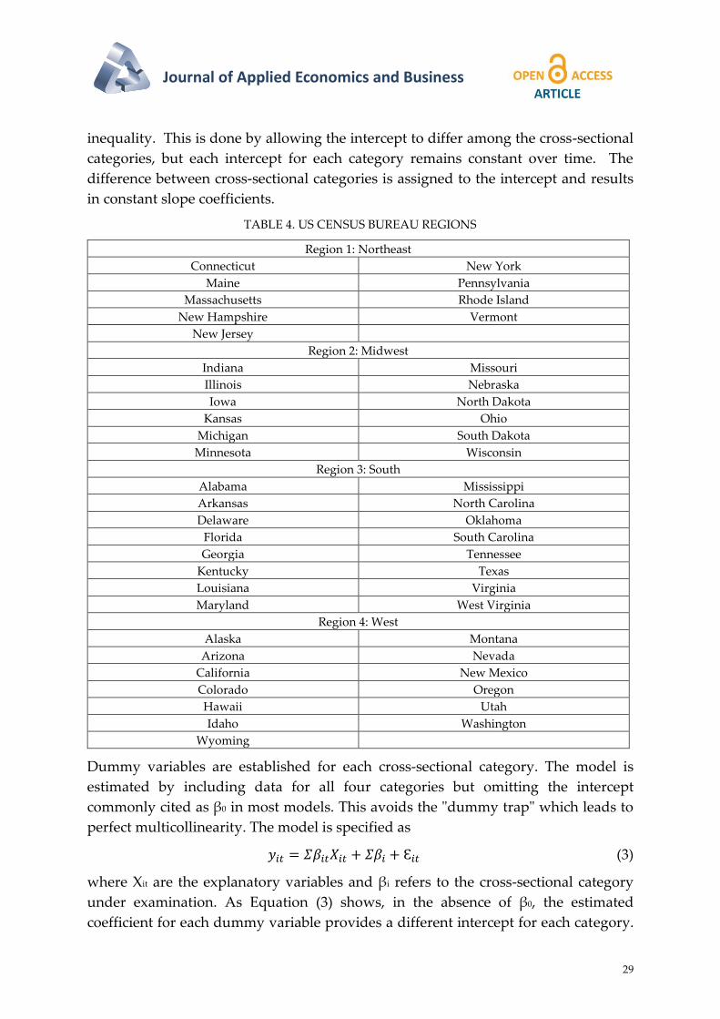
inequality. This is done by allowing the intercept to differ among the cross-sectional

categories, but each intercept for each category remains constant over time. The

difference between cross-sectional categories is assigned to the intercept and results

in constant slope coefficients.

TABLE 4. US CENSUS BUREAU REGIONS

Region 1: Northeast

Connecticut New York

Maine Pennsylvania

Massachusetts Rhode Island

New Hampshire Vermont

New Jersey

Region 2: Midwest

Indiana Missouri

Illinois Nebraska

Iowa North Dakota

Kansas Ohio

Michigan South Dakota

Minnesota Wisconsin

Region 3: South

Alabama Mississippi

Arkansas North Carolina

Delaware Oklahoma

Florida South Carolina

Georgia Tennessee

Kentucky Texas

Louisiana Virginia

Maryland West Virginia

Region 4: West

Alaska Montana

Arizona Nevada

California New Mexico

Colorado Oregon

Hawaii Utah

Idaho Washington

Wyoming

Dummy variables are established for each cross-sectional category. The model is

estimated by including data for all four categories but omitting the intercept

commonly cited as β0 in most models. This avoids the "dummy trap" which leads to

perfect multicollinearity. The model is specified as

𝑦𝑖𝑡 = 𝛴𝛽𝑖𝑡𝑋𝑖𝑡 + 𝛴𝛽𝑖 + Ɛ𝑖𝑡 (3)

where Xit are the explanatory variables and βi refers to the cross-sectional category

under examination. As Equation (3) shows, in the absence of β0, the estimated

coefficient for each dummy variable provides a different intercept for each category.



The resulting intercepts allow the model to reflect differences among the different

categories.

The fixed-effects model permits the distinct advantage of allowing all data to be used

in the regression rather than just those just pertaining to a specific category as is the

case with seemingly unrelated regression models (SUR). This permits a larger number

of degrees of freedom and is thus likely to be more accurate.

Further, the dummy coefficients for the SUR models can avoid multicollinearity by

excluding one of the dummy variables. The ensuing coefficients for the remaining

dummy variables represent the change in the intercept when the category is compared

to the omitted dummy variable. Since the purpose of this experiment is to capture

differences among four census bureau regions, it seems a fixed-effects model is more

appropriate. The intent of the fixed effects model is to determine if the intercepts are

the same for all four regions. If they are, a fixed-effects model is unnecessary. The

determination is based on a hypothesis test framed as

Ho: βNorth = βMidwest = βSouth = β West

Ha: Not all βi are Equal

The appropriate methodology requires an F-test containing values derived from the

results of two regression models: a restricted model and unrestricted model. The

restricted model does not include a dummy variable for region and contains the

constant term, β0. It is expressed as

𝑌 = 𝛽0 + 𝛴𝛽𝑖𝑡𝑋𝑖𝑡 + Ɛ𝑖𝑡 (4)

By excluding any reference to the different regions and including a single value for β0,

it restricts the four intercepts to equality. The unrestricted model is the fixed-effects

model seen as Equation (3). The F-test is calculated as

𝐹 =

𝑅𝑆𝑆𝑅 − 𝑅𝑆𝑆𝑈

𝑞𝑅𝑆𝑆𝑈

𝑛 − 𝑘 − 1

(5)

where RSSR is the residual sum of squares for the restricted model and RSSU is the

residual sum of squares for the unrestricted model. q is the number of restrictions

contained in the null hypothesis and equals the number of parametric coefficients set

equal to each other. n is the number of observations and k is the number of right-hand

side variables in the unrestricted model. Expressed in this manner, the F-statistic

measures any improvement in the fit offered by the unrestricted model over that

reported by the restricted form.

RSSR will always be more than RSSU because some of the variables in the restricted

model are constrained and cannot fit the data as well as the unconstrained model.

Furthermore, the unrestrained model contains more explanatory variables and will

offer a better fit. Consequently, the F-statistic is always positive.


31

In this present case, q is 4, n is 50 and k = 7. Computations produce an F-value of 3.41

and a p-value of 0.0167. The null hypothesis that the intercepts for all four regions are

equal is rejected at the 1.67% level of significance. Clearly, the nature of the

relationship between economic freedom and income distribution varies across state

boundaries in the US.

Given the cross-sectional nature of the data set, White’s test for heteroscedasticity

(1980) as modified in Webster (2013) was conducted. Unlike other tests for

heteroscedasticity, White's test as modified does not require that the variables

proportionally associated with the heteroscedastic variances be identified. Instead, all

right-hand side variables used in the fixed-effects specification, and several in their

modified forms, are used in the detection method. For example, if the initial regression

model carried k regressors, White’s test requires the application of Equation (6). The

squared residuals from the restricted model are used as the regressand. They are

regressed on a battery of potential explanatory variables.

𝑒2 = 𝛽𝑜 + 𝛽𝑖𝑋𝑖𝑡 + 𝛽𝑖𝑌𝑖𝑡 + ⋯ + 𝛽𝑖𝑘𝑖𝑡 + 𝛽𝑖𝑋𝑖𝑡2 + 𝛽𝑖𝑌𝑖𝑡

2

+ ⋯ + 𝛽𝑖𝑘𝑖𝑡2 + 𝛽𝑖𝑋𝑖𝑡𝑌𝑖𝑡 + 𝛽𝑖𝑋𝑖𝑡𝑘𝑖𝑡 + 𝛽𝑖𝑌𝑖𝑡𝑘𝑖𝑡 + 𝜛 (6)

Four explanatory variables are used in the restricted model: Gini2000, EFI2000, EFI2013 and

the change in the Gini ratio from 2000 to 2013. There are therefore 14 regressors in

Equation (6). Testing for heteroscedasticity via this method requires the computation

of nR2 where R2 is taken from Equation (6). This statistic fits a χ2 distribution that is

used to test the hypothesis that all βi in Equation (6) are zero. If the null hypothesis is

not rejected, it may be concluded that constant error variance prevails and the model

is not plagued by heteroscadasticity. The R2 from Equation (6) is 0.206. With n = 50,

nR2 = 10.32. Testing the hypothesis at the 5% level of significance, the critical χ.05,14 =

23.68. Since 10.32 < 23.68, the hypothesis of constant error variance is not rejected. It

would appear that the model does not suffer from heteroscadasticity. The Durbin-

Watson reported as 1.89 indicating no obstruction due to autocorrelation.

TABLE 5. FIXED-EFFECTS REGRESSION RESULTS; CHANGE IN GINI AS REGRESSAND

Results of the Fixed-Effects Model With Gini2013 as Response Variable


Gini2000 0.2079 0.0407 5.11 0.000

EFI2013 -0.0048 0.0026 -1.78 0.082

EFI2000 -0.0230 0.0062 -3.73 0.001

Change in EFI -0.0058 0.0012 -4.83 0.000

NORTHEAST -0.0557

MIDWEST -0.5599

SOUTH -0.6190

WEST -0.06190



The results shown in Table 5 are clear and unequivocal. The coefficient for EFI for 2013

is negative and significant. This reveals that states with greater economic freedom in

2013 are going to exhibit greater income equality. This negative correlation attests to

the impact economic freedom has on the distribution of income in any geographical

unit.

The same interpretation can be applied to the EFI for the year 2000. Here again we

find a significant, negative relationship. States displaying pronounced economic

freedom at the outset of the time period under examination will report less income

inequality later on. It may be concluded that economic freedom as provided by the

Fraser Institute promotes greater income equality as measured by the Gini coefficient.

The initial Gini ratio is highly significant and carries a positive sign. This indicates that

states exhibiting a high degree of income inequality in the year 2000 will continue to

experience this condition over time.

TESTS FOR CAUSALITY

A reasonable question focuses on any causal relationship that might exist between

income distribution and economic freedom. Therefore, a Granger causality test is

offered to test for directional causality between these two socio-economic variables.

This test is performed to determine if any past values of one variable may affect

present values of a second variable. That is, to address the question as to whether past

values of X serve as explanatory variables of Y. Y is then regressed on past (lagged)

values of itself as well as lagged values of X. The question as to how many lagged

values of each variable should be included in the model is paramount.

It is imperative that the data used in the analysis prove to be stationary and do not

exhibit a unit root. Initially, the test for a unit root is based on the Equation (7) such

that

𝑌𝑡 = 𝜌𝑌𝑡−1 + µ𝑡 (7)

where it is assumed -1 ≤ ρ ≤ +1 and µt is merely white noise. If ρ = 1, (7) is a

nonstationary random walk or stochastic process without drift and cannot be

effectively estimated.

It would seem reasonable to then simply test the null hypothesis that ρ =1 against the

alternative hypothesis that ρ < 1. This is written as a one-sided test because if ρ > 1,

the series is said to be explosive and thus difficult to model. Besides, explosive series

of this nature are quite uncommon using economic data due to the cyclical nature of

economic activity. If the null is not rejected the series carries a unit root and is

nonstationary. That is, if ρ = 1, it may be concluded that a unit root prevails and a

random walk model without drift results thereby evidencing a nonstationary

condition.


33

However, such a test is not possible since if a unit root exists the t-tests produce biased

results. Specifically, the t-values for the coefficient of Yt-1 do not follow an asymptotic

normal distribution even in the presence of large samples.

It is therefore necessary to find an alternative approach to test for unit root. Perhaps

the most common approach is that provided by Dickey-Fuller (1979). The Dickey-

Fuller test (DF) is applied by subtracting Yt-1 from both sides yielding Equation (8).

𝑌𝑡 − 𝑌𝑡−1 = 𝜌𝑌𝑡 − 𝑌𝑡−1 + µ𝑡

𝑌𝑡 − 𝑌𝑡−1 = (𝜌 − 1)𝑌𝑡−1 + µ𝑡 (8)

If Yt – Yt-1 is shown as ΔYt and δ is set equal to (ρ – 1), we have

ΔYt-1 = δYt-1 + µt (9)

The equivalent test then carries a null hypothesis of δ = 0 with the alternative stated

as δ < 0. Since δ = (ρ – 1), for ρ < 1 and avoid the unit root, δ must be less than zero. If

the null that δ = 0 is not rejected, ρ = 1 and nonstationarity in the series exists making

it difficult to conduct any causality test. The t-value used in this hypothesis test is then

compared not to the standard t-distribution, but that provided by Fuller (1976) used

exclusively for this particular test. Appling Equation (9) to both income inequality and

EFI failed to lead to a rejection of the null hypotheses. Thus, it is concluded both suffer

unit roots requiring corrective action.

The most common practice is to first-difference the series. Generally, the first

differences of time-series are stationary. To determine this, the first differences are

taken for both variables and then Equation (9) is applied to those first differences.

Both tests for income inequality and economic freedom suggest stationarity.

The Granger causality test can then be applied to these first differences. The complete

Granger test for Y and X, for example, involves the comparison of two regressions

models, the restricted model and the unrestricted model. To test whether X Granger-

causes Y, the restricted model is expressed as

𝛥𝑌𝑡 = 𝛼𝑡 + ∑ 𝛼𝑖𝑌𝑡−𝑖 + µ𝑡 (10)

𝑝

𝑖=1

This is referred to as the restricted model because it contains no reference to the X

variable. The coefficients for X are assumed restricted to zero and are therefore held

out of the model.

In the absence of more sophisticated computer software that will identify the optimum

number of lags, it is advisable to begin with a large number of lags and test for

significance in succession starting with the oldest values (largest lags).

The unrestricted model is



𝛥𝑌 = 𝜙𝑡 + ∑ 𝜙𝑖

𝑝

𝑖=1

𝑌𝑡−1 + ∑ 𝛽𝑖𝑋𝑡−𝑖 + 𝜈𝑡

𝑞

𝑖=0

(11)

Here the coefficients for X are not assumed to be zero. If that is so, then past values of

X Granger-cause changes in Y.

The null hypothesis is that past values of X do not Granger-cause changes in Y. The

null is expressed as Ho: βi = 0. If the null is not rejected, it may be concluded that X

does not Granger-cause changes in Y.

To test for causality from Y to X, Equations (10) and (11) are reversed setting X as the

dependent variable. The same hypothesis test is then performed on this second set of

equations.

Final determination is based on the standard Wald F-test that offers a comparison

between the restricted and unrestricted estimates as shown by Equation (12).

𝐹 =

𝑆𝑆𝐸𝑅 − 𝑆𝑆𝐸𝑈

𝑞𝑆𝑆𝐸𝑈

𝑛 − 𝑝 − 𝑞

(12)

where SSER and SSEU are the sums of the squared residuals for the restricted and the

unrestricted model, n is the number of observations, p and q are in the number of lags

in the dependent and independent variables, respectively. The result is compared to

a critical F-value with q and n-p-q degrees of freedom.

Four possible outcomes may result. It may be determined that Y Granger-causes X, X

Granger-causes Y, there is bilateral causation in that each Granger-causes the other or

the two variables may be independent in which neither Granger-causes the other.

After considerable tests to detect significance in lagged values based on the current

data set, it was determined that a lag order of three was appropriate for both variables

in both tests. A test was first conducted to determine if income inequality might

Granger-cause measured levels of economic liberty to vary. That is, the EFI was used

as the regressand for both the restricted and unrestricted models. An F-value of 1.14

was reported. This value is below any acceptable critical F-value for this test and

carried a p-value of 0.389. It may be concluded that the null hypothesis that income

distribution does not Granger-cause economic freedom cannot be rejected. It would

appear that there is no directional causality running from income inequality to the

freedom index. Past measures of income distribution do not offer any explanatory

value for changes in the levels of economic freedom.

Treating income inequality as the dependent variable and using the EFI as the

regressor yielded an F-value of 7.25. The associated p-value is 0.0114 allowing a

rejection of the null hypothesis that economic freedom does not Granger-cause

changes in income distribution. It may be concluded that past levels of economic


35

freedom Granger-cause changes in the degree of income distribution as measured by

the Gini coefficient. The significant coefficients for lagged values of the EFI all report

negative signs and thereby contend that prevailing measures of economic freedom

will in the near future lead to greater economic liberty within the populace.

CONCLUSION

The results presented here suggest that elevated measures of economic freedom are

associated with more equal distributions of income. This pattern holds true at specific

points in time as well as dynamics measured over the past decade. After controlling

for other factors, the Gini ratio for the year 2000 exhibits a negative relationship with

the EFI for the same year. Given that increases in the Gini coefficient evidence lower

levels of income equality, it may be concluded that in regions with greater measures

of economic freedom, a drop in the Gini suggests greater income equality. Incomes

become more evenly distributed in areas where economic participants are given

greater discretion in their activities in the prevailing economic markets.

These findings seem to run contrary to those reported by Ashby and Sobel (2008).

Their paper did not find that measures of economic freedom were negatively related

to increased levels of inequality. Perhaps this discord results from the different time

periods used in the two studies.

Virtually identical results were found when more recent measures were used in the

OLS models. Regressing the Gini coefficient from 2013 on the EFI for the same year

suggested again that economic freedom was associated with a more equitable

distribution of incomes across the states. These results also conflict with those

presented by Ashby and Sobel (2008) but tend to support the findings based on studies

comparing different nations around the globe as noted above.

With respect to an examination of the effect of changes in income dispersion over time,

we find much a greater degree of accord. This paper demonstrates that changes in the

levels of income equality are significantly associated with changes in the degree of

economic freedom. Specifically, the change in the Gini over the time span of 2000 to

2013 reported a negative relationship with both the EFI in 2000 as well as EFI2013.

Further, the change in that index over the same time period reported a negative

relationship with the change in the EFI. This reveals that greater equality can be

nurtured by efforts to foster enhanced economic freedom within the economic climate.

This conclusion does tend to correspond with that provided by Ashby and Sobel

(2008), as well as those presented by Berggren (1999) and Barro (2000).

The fixed-effects model clearly indicated the nature of the relationship between

economic freedom and income distribution varies across state boundaries in the US.



Differences among the four US Census Bureau regions in terms of the industrial mix,

general economic climate, public policies and the host of other socio-economic factors

might explain these differences. Further research should be conducted to determine

what attributes and qualities characteristic of the regions are most conducive to

promoting this relationship between economic freedom and a more equitable

distribution of income.

Certainly, before any firm theoretical foundations can be formulated, additional

research into the pressing issue is necessary. Despite the recognized trend in income

distribution in the US over the past several decades, it is only recently that concern

has been raised as to the consequences such patterned changes might have on our

social, economic and political fabric.

It seems self-evident that the current drift in the pattern of income distribution cannot

and should not be sustained. The consequences could lead to a regrettable outcome.

If effective public policy is to be enacted, a greater understanding of the interaction

and dynamics among the forces discussed in this paper is essential.

After correction for non-stationarity using the Dickey-Fuller test and applying first-

differencing, the Granger-causality procedure was applied to the data to detect the

whether there was any feedback between income measures and the existing degrees

of economic liberty as measured by the Economic Freedom Index. It was clearly

determined that while earlier measures of income distribution could did not appear

to Granger-cause and changes in economic freedom. However, such was not the case

for the opposing test. Past measures of the Economic Freedom Index proved to be high

significant as explanatory factors for changes in income distribution.

REFERENCES

Apergis, N., Dincer, O. & Payne, J. (2011). On the Dynamics of Poverty and Income

Inequality in US States. Journal of Economic Studies, 38, 132-143.

Barro, R. J. (2000). Inequality and Growth in a Panel of Countries. Journal of Economic

Growth, 5, 5-32.

Berggren, N. (1999). Economic Freedom and Equality: Friends or Foes?. Public Choice,

100, 203-223.

Card, D. & Lemieux, T. (2004). Unions and Wage Inequality. Journal of Labor

Research, 25(4), 519-559.

Cebula, R. J., Clark, J. R. & Mixon, F. G. Jr. (2013). The Impact of Economic Freedom

on Per Capita Real GNP: A Study of OECD Nations. Journal of Regional Analysis and

Policy, 43(1), 34-41.


37

Dickey, D. & Fuller, W.A. (1979). Distribution Of The Estimators For Autoregressive

Time Series With A Unit Root. Journal of the American Statistical Association, 74, 427-

431.

Fuller, W. A. (1976). Introduction to Statistical Time Series, New York: Wiley.

Gini, C. (1997). Concentration and dependency ratios. Rivista di Politica Economica,

87, 769-789.

Gwartney, J., Lawson, R. & Block, W. (1996). Economic Freedom of the World: 1975-

1995, Vancouver, Canada: Fraser Institute.

Piketty, T. (2014). Capital in the Twenty-First Century, The Belknap Press of Harvard

University: Cambridge, MA.

Piketty, T. & Saez, E. (2003). Income Inequality in the United States. Quarterly Journal

of Economics, 118(1), 1-39.

Ram, R. (2012). Social Capital and Income Inequality in the United States. Atlanta

Economic Journal, 41, 89-91.

Scully, G. (2002). Economic Freedom, Government Policy and the Trade-Off between

Equity and Economic Growth. Public Choice, 113, 77-96.

Sommeiller, E. & Price, M. (2014). The Increasingly Unequal States of America: Income

Inequality by State, 1917 To 2011, Economic Policy Institute, Report: Inequality and

Poverty.

Spindler, Z., X. de Vanssay & Hilderbrand, V. (2008). Using Economic Freedom

Indexes as Policy Indicators: An International Example. Public Organization Review,

8(3), 195-214.

US Department of Labor: Bureau of Labor Statistics (January 24, 2014), Union

Members Summary: Economic News Release; http://www.bls.gov/news.release/

union2.nr0.htm; (Extracted December 19, 2014).

Webster, A. (2014). An Examination of the Growing Level of Income Inequality.

American Journal of Economics and Business Administration, 6(1), 11-18.

Webster, A. (2013). The Relationship between Economic Freedom and Income

Equality in the United States. International Business and Economics Research Journal,

12(3), 469-475.

Webster, A. (2013). Introductory Regression Analysis: With Computer Applications

for Business and Economics, Routledge (237-238).

Western, B. & Rosenfeld, J. (2011). Unions, Norms, and the Rise in US: Wage

Inequality. American Sociological Review, 76(4), 513-537.



White, H. (1980). A Heteroscedasticy-Consistant Covariance Matrix Estimator and a

Direct Test for Heteroscadasticity. Econometrica, 48(4), 817-838.


39

HUMAN RESOURCES IN THE

INTERNATIONAL ORGANIZATION’S

CONTEXT


Abstract

Why do firms engage in international business? This happens for three main reasons: (i) To expand

their sales; (ii) To identify new resources; and (iii) To diversify the sale and supply resources.

Undoubtedly we are becoming further more convinced on the key role the human resources play in

any organization, especially in the international organization. If human resources require a

considerable attention in the firms operating within the country, it is rather easy to imagine the degree

of indispensable attention they need in the firms operating in a global context. In this context, the

company leaders are faced with the need to perform their work activity through the efforts of local

employees, foreign employees, agents and suppliers. By creating strategic alliances or international

joint ventures, the boundaries and organizational relationships (sub-contracted, part-time

employments) are prone to change, thus these circumstanced call to attention the regulation of the

workforce, aiming at achievement of the objectives in the global context. In order to obtain some

valuable conclusions concerning the human resource management, waging research and engaging in

the use of particular resources, becomes a necessary process to be undertaken. Moreover, as this topic

has been a vital issue, it has gained the attention of numerous researchers who have made hypotheses

or build models on human resources in the international organizations context. What has particularly

attracted my attention is the individual in itself, the manager working in an international organization,

the one transferred to work in a branch of an organization for a relatively long period. I was eager to

know his perspective on the experiences, how has his/her way of thinking changed, his/ her lifestyle;

would he/she be willing to go back to his workplace etc.? Another interesting issue is being able to

comprehend the organization’s perspective, the procedures applied to selects the appropriate

employees performing a specific job, how does the organization implements the human resource

planning, which is the recruitment strategy effectuated, who are the selected employees to be

transferred, what is the applied model in making the due selection?

Key words

Global context; Regulation; Transference; Human resource management; Diversification.


Human Resources in the International Organization’s Context


INDIVIDUAL CAREER IN THE INTERNATIONAL CONTEXT

The management career, particularly in these modern times stretches outside the

traditional environments. This has resulted due to the business globalization, which

in turn has brought about the need to attract and retain the most suitable employee in

relation to an organization’s culture. The transfer of career managers has increased

furthermore the analysis on this case. Various economists have spoken out different

arguments. They have tried to start the analysis within family grounds: how many

individuals have been transferred due to work-related reasons? What their reactions

were, concerning the workplace adjustment? Which were the problems encountered

and have they been of a transitory nature or not? The studies also bring help

concerning the career management in the international context. In this regard, it is

worth mentioning that all managers experience difficulties when transferred from one

working place to another due to the cultural variations (Birdseye & Hill, 1995).

This can be a cause of many reasons, such as:

1. At the first moment, the manager himself may have asked the transfer due to

qualification reasons, but the cultural differences have hindered him/her to

proceed further; and

2. Another reason might be the fact that he/she fails to accept the firm's strategy

in an international configuration. Probably the staff that he/she is supposed to

work with brings about difficulties; it might happen that the staff might not fit

in the international business policies presented by the newcomer.

Managers also need to adapt to the specific cultural requirements of the international

environments where they are supposed to work. This can also result a damaging

practice to them. Rationally, the human resource management is inevitably connected

to the organization’s development level. Therefore, for each and any single movement,

we must always bear in mind the dual relationship manager –company, and when it

comes to the manager, we shall consider his/her career. This is the only viable way to

create valuable models based on the management concepts. We confer to this because

the transfers from one country to another will instigate individual ideas to the

manager, making him/her prone to be selective with regard to one country compared

to another in order to increase his/her career chances. Thus he/she makes differences

depending on the environment judged as culturally fit, given the fact that companies

are always in search of the maximum adjustment basis, because they aspire their

ongoing development. In fact, the internationally operating organizations have not

granted the due significance to those managers intending to establish an international

career in their management practices. Normally such initiatives must be included in

an international career development program, at the moment when the appropriate

staff will be recruited.


41

In addition, there are other attention-seeking issues related to the international career

management, which could help in the strategic management of business enterprises,

improve the HRM practices in general and address the needs of career personnel

involved in the process. According to Sonnenfeld et al, (2006: 588) ‘The practice has

failed to correctly address the organization's requirements in the human resource

management’.

THE GLOBAL BUSINESS STRATEGIES LINKS TO THE RECRUITMENT

MODEL

The global management strategies in multinational companies vary greatly. The

processes, practices, systems and the developed structures to implement these

strategies will also vary. Developing global strategies can prove difficult, given the

conflicting or contradictory environments wherein the multinational company may

operate (MNC). Requirements often arise due to MNC's efforts to maximize their

capacity to respond to the needs in host countries (local reaction), trying to maintain

or keep under control world widely their corporation structure in order to establish a

global integration. In often-cases, branches may have more autonomy acting

independently and in order to respond to local requirements, remain less integrated

as an international organization (Prahalad & Doz, 1987 missing; Tung & Punnett,

1993). The above theory has not undergone much changes since 1970, however Adler

and Ghadar (1990) performed their duty in classifying MNC strategies on

management skills. Recently, these strategies are being reconceived in terms of MNC

life cycle in accordance with the product’s generation, sales and development stages,

under the symbol of Adler and Ghadar (1990), and Milliman et al, (1991). By applying

the life cycle model or the classification model, the strategies are certainly involved in

the global management and interoperability.

In the MNC’s management phases, of vital importance is the local responsibility. As a

result of study integration and accountability there are mentioned four strategies:

i. Ethnocentric

ii. Polycentric

iii. Local (region-centric)

iv. Geocentric

In general terms, these four stages in the Human Resources Management literature

correspond to internal, in terms related to the phase 1; the phase 2 and phase 3 relate

to International and Multinational dimensions and phase 4 is the Global stage.




Generally speaking, the ethnocentric strategy suggests that companies should

maximize control over branches, in order to have an integration of their own and

manage to minimize costs. In the polycentric and region-centric cases, local reaction

is far more present and sensitive and is noticeable even less integration within the

corporate. Geocentric strategy is the ideal and it tends to balance and responsiveness

of local and global integration simultaneously. If we will dare to trace the

phenomenon in basic hierarchical grounds, the geocentric strategy would prove a

good choice as it envelopes two theoretical ideals. The Polycentric and region-centric

strategies would rank as the second-best strategies because they remain more

concentrated in accomplishing the local perspectives. Meanwhile the ethnocentric

strategies, bearing the main focus in controlling, are either globally or locally

integrated. In general, as foreign branches mature, they become a more independent

source, regarding the strategic resources such as technology, capital, management, or

approaches to markets. If they seek dependence upon the mother-organization, on the

purpose of performing controls, then it’s indispensable for them to change the

autonomy terms, or to utilize alternative methods in order to promote their activity,

ranging from the interrelationship with the mother-company, to the world wide

operation. The rate at which MNCs aspire that their employees world widely share

their corporate culture and also socialize with the employees in the host country,

transmitting them the mother-corporation culture, will be evidenced via the processes

and the allocation of the socialization assigned resources. We may mention such

methods as, sending migrants abroad to spread the corporate culture, selecting

individuals that share the organization’s values, bringing the host country citizens in

the country of origin in order to gain know-how etc.

The ethnocentric practices on immigrants, as part of the mother branch personnel, will

be centered on their management and will be more focused on the controls and

decision making by the mother branch. This happens more when the branches are

managed from the center. Such practices are more common when the management is

waged by the center-organization. This ethnocentric approach is more usual at the

start of an enterprise and in case when special technical capacities are necessary when

they can be found in the local workforce. However, the international human resource

management is the responsible mechanism finding the suitable immigrants who will

prove successful abroad. Current literature suggests that there is an extremely high

turnover rate among the immigrants and that success on the abroad transference

requires a unique set of skills and capabilities above and beyond the usual technical

skills needed for the analogous position in the home-organization. The transference

costs are too high and moreover the respective laws applying are far astringent.

Consequently in often cases, accommodating their families depend on the help of the

mother-company. The ethnocentric multinational corporations expect their leaders

sent to foreign countries to transfer their culture and to demonstrate the most efficient

management practices of the multinational and/or international corporation. There


43

are other cases that the mother company sends individuals to foreign countries and

these individuals socialize with the host country employees far than usual. Thus, a

greater socialization is reached based on desire. The reason under this conclusion is

that, the structure of the host national company is not directly affected by the mother-

company.

Some data show that even when the mother company has sent staff in order to

transmit its culture to the branches, still the branch culture has prevailed over the

mother company. The polycentric and region-centric practices regarding the

international human resource management are based on the approach undertaken

into how to manage and administer the branches’ activity from the headquarters of

the mother-company. For those companies having branches in various host countries,

all the managerial phases are performed by the locals and rarely are noticed cases of

transferred personnel from the mother-company. In this case, the company cuts on

expenses, compared to the transference of staff from the mother-company. However,

the mother-company is willing and open to gain valuable global perspectives form the

abroad employees and it is also in the known that the employees not always can

socialize to the mother company culture. This can be accomplished either through

transference of this staff in the native country to gain experience, or via sending

representatives from the mother company to the country wherein the branch will be

settled. For this reason, being that the cultural alignment does not happen overnight,

the very career of the managers and employees of the company in the host country

cannot reach the highest level, therefore it’s harder for them to take over management

level posts in the mother-company. The polycentric companies experience a concern

regarding the common culture of the company’s management.

A similar management strategy to the polycentric approach is the geocentric one.

From this perspective, the employees of the host countries and the third countries can

be recruited and/or selected to work on a regional basis. The regions’ selections should

go in consistency to some indispensable elements as the natural border, such as the

European Economic Community or the Middle East. In the region-centric MNCs, the

communication systems and the very integration must be highly sophisticated on the

part of the mother-company, in order to maintain control over the regions in which it

operates. In the polycentric perspective, the career chances of the national staff of the

host country are higher to progress within the region, but it occurs that success can be

attained even with regard to the mother company. However, as happens in

organizations having a multitude of polycentric perspective, the local citizens are

given the opportunity to manage their own branches. The geocentric practices of HRM

and MNCs aim at an all-comprehensive integration of all their branches and a merge

of the world-wide cultures, thereof they need to adopt a geocentric strategy. MNCs




effectuate the adoption of this strategy in a worldwide scenario, intending to attract

the most qualified individuals working in various positions, irrespective of their

nationality. When talking about MNC's geocentric creations, we view the situation as

being the case of company’s integration in global terms, experiencing a cultural

unification of companies, but not necessarily dictated by the mother-company. There

are other cases of a more complex organization of the geocentric companies. In this

case the structure is substantially pivotal, as it requires an extensive communication

and integration of workers even across borders. In the case of geocentric MNCs, the

socialization of the organization’s values is employed as a strategy ruled by flexibility,

in order to accommodate as good as possible the needs of the daughter company, in

order to feel as comfortable as possible working in a country with a different culture

from their country of origin. Despite this fact there will always be cultural differences.

However, they will always attempt to acquire the values, attitudes, cultural norms of

the country where they are working. This is done through the contacts with the

mother-company and other foreign branches, the transfers and various visits to other

foreign countries in order to develop global links. Given that this strategy is carried

out through trainings organized in the mother company or in branches, it allows the

greatest amount of local trials and decentralization level, thus to maintain the overall

integration.

A considerable part of literature treats the socializing approaches or the strategic

socialization. To make employees feel good, transference bonuses are often provided,

as show ticket, different invitations, in order for them to adapt as easily as possible to

the new country. Frequently, decent living conditions are provided to their families.

If the transference is scheduled for a long time and the assignment is at a managerial

level, then better conditions are provided in order to facilitate transference adaptation

process. The adaptation processes are intended so that the employees may

acknowledge not only the culture of the MNC mother organization country, but also

the culture of the countries where MNC operates. The main objective is to somehow

neutralize national culture features and to attempt to comprise it in the MNC's culture.

This is the basic theory applied in strategic human resource management of MNC's.

Edstrom and Galbraith (1977), noted that the theoretical grounds of their studies

provide a framework for examination; afterwards we can move on to evaluating the

work validity of the international strategic management of human resources. In line

with what was discussed above, we may have a dual representation regarding the

decision to preserve culture. There may be cases of MNC who want to preserve the

mother-company culture, but also there may be cases of MNCs which select the

polycentric approach, that is to take into consideration the host countries’ culture.

Also, the geocentric operating companies are less concerned with the mother company

culture preservation, compared to the region-centric, the polycentric or the

ethnocentric. The ethnocentric companies recruit globally less foreign workers

compared to the region-centric and geocentric companies. Especially in geocentric


45

companies the global recruitment approaches are widely practiced. The ethnocentric

companies will retain less their selection standards worldwide compared to the

polycentric, region-centric and geocentric MNCs, due to the fact that they prefer to

make selection within the mother country. In the case of ethnocentric companies most

of the time they tend to contact with their employees, as they strive to settle closer

relationships compared to the region-centric and geocentric companies. Nevertheless,

these companies do have social policies used exclusively to improve the individual

performance. In the firms organization there are delineated a multitude of

international strategies, created to the sole aim of achieving the economic success.

From the human resources perspective, the geocentric MNC 's target is to attract the

most appropriate employees in order to choose among them the best and most

talented. This is vital in those cases where the position is of key importance. In these

cases not only the best applicant will be selected, but he/she will be gratified with all

the required conditions in order to result in the most productive. The affinity the

geocentric MNCs have to human resource structures is of more strategic nature, thus

it gives them significant competitive advantages. In addition, these employees will

gain global perspectives and international capacities, which will further strengthen

MNCs in all their activities.

An important issue for discussion is the MNC’s management of high level positions

strategy and its efficiency in a single line. Despite the good initiatives the big

companies may have in regulating their activities worldwide and the best recruitment

they can select, they are still faced with hurdles. Starting from the legal practices in

host countries, to the political and cultural differences, which in turn can cause

adjustment problems. Finding the appropriate solution is the responsibility of the

international human resources, which in an organized manner should develop

practices in conformity with the legal, political and cultural grounds, thus it is better

achieved the most appropriate adaptation. In this case even the employee is well

aware of where he/she is going, the surrounding environment expected to be found,

on the other hand the local employee is provided the due information on foreigners

arriving. In the same way the host employee is prepared, similarly the foreign

employee to be transferred gets prepared in order to acknowledge the culture, politics

and the legal regulations of the country, where the mother company operates.

The involvement of human resources in both preparatory stages will create the

opportunity that the international human resource management may function

effectively in a global context. Regarding the ways through which the company

recruits its employees, always in conformity with its strategies chosen to operate the

below recruitment approaches are recognized:

i. Geographical recruitment; and




ii. Internal versus external recruitment.

The target of the geographical recruitment in searching for potential candidates might

be extended in the global context if the company is following a geocentric strategy and

is looking for the best talents in an international context. International firms, in cases

of middle to low level management recruitment, decide to wage the recruitment

selection in the bulk of the host country applications. However MNCs as Merck, 3M

and IBM encourage the internal recruitment, following the Promotion Policy from

within the company in the mother-country, as well as in the host country.

This is done because some conspicuous advantages are noticed:

i. When using an effective human resources information system, the most suitable

candidates are more easily found saving time and cutting costs for research.

ii. Having such an efficient system, the possibility to increase the selection

decisions validity is undoubtedly increased and made highly ‘readable’.

iii. Promotion from within the company is an immediate indicator of the

considerable level of retention and productivity and the promoted employees will

view internal recruitment as a promise for career advancement within the

organization.

iv. A major advantage is the fact that the existing employees do not need training

because they know far better the operational policy and the company culture

compared to a newcomer.

Harvey and Novicevik (2001) added these advantages to the list:

i. Internal candidates are easier to persuade in taking an assignment abroad.

ii. Since the internal candidates are far more familiar with the company culture,

they know better the ways of internationalizing their careers.

iii. Internal candidates are more reliable in cases of expansion of control units,

regarding the global operations.

On the other hand the external recruitment brings about several advantages, amongst

which we can mention:

i. Brings in new ideas and new perspectives within the organization.

ii. Reduces the training costs when technically trained employees are recruited.

iii. Enables a greater, additional human resources work power, especially in

expansion periods without being forced to tantalize the current internal staff.

iv. Facilitates objectivity and flexibility to make critical decisions without

depending on previous experiences or past built relationships.


47

Despite the above mentioned advantages, there are considerable obstacles related to

external recruitment, starting from the newcomer costs, to the organization culture

adaptation.

CONCLUSIONS

The human resource recruitment process is simultaneously a vitally professional

depended process, and regionally bound. In order to wage the most appropriate

recruitment strategies, especially the companies operating in an international context

need to take care primarily of the mother-company needs and principles to be adhered

to, and secondly for the daughter-company success. The process is greatly aided by

the transference of the know-how from the mother-company to the respective

branches, and on the other hand by building capacity in the host country.

Various strategies are employed in attaining the objective, starting from the

ethnocentric to the polycentric, from the local (region-centric) to the geocentric, each

and every single of them bearing their pros and cons when it comes to their

application and a successful projection depends on the regional grounds, the

professional needs, the technical requirements etc.

Nevertheless is up to the MNCs capacity to decide upon ‘casting’ the appropriate

amount of responsibility to the daughter-company. As a result of study integration

and accountability there are mentioned four strategies (Ethnocentric, Polycentric,

Local (region-centric) and Geocentric).

In drawing comparisons the ethnocentric strategy suggests that maximum control

over branches is indispensable in order to create integration and minimize costs. The

polycentric and region-centric approaches admit that the local reaction is far more

present and noticeable. Meanwhile the geocentric strategy is the ideal combination

and it strives to simultaneously balance the local responsiveness to the global

integration.

REFERENCES

Birdseye, M. G. & Hill, J. S. (1995). Individual, Organizational; Work and Environmental

Influences on Expatriate Turnover Tendencies: An Empirical Study. Journal of International

Business Studies, 26(4), 507-529.

Prahalad, C. K. & Doz, Y. (1987). The Multinational Mission: Balancing Local Demands and

Global Vision. Free Press, New York.




Tung, R. L. & Punnett, B. J. (1993). The Relationship of Staffing Practices to Organizational

Level Measures of Performance, Personnel Psychology, 46, 27-48.

Adler, N. J. & Ghadar, F. (1990). Strategic Human Resource Management: A Global

Perspective. In: Pieper, R. (Ed.) Human Resource Management: An International Comparison,

235-260.

Edstrom, A. & Gialhraith, J. R. (1977). Transfer of Managers as a Co-ordination and Control

Strategy in Multinational Organizations. Administrative Science Quarterly, 22, 248-263.

Milliman, J., Von Glinow, M. A. & Nathan. M. (1991). Organizational life cycles and strategic

international human resource management in multinational companies: Implications for

Congruence Theory. Academy of Management Review, 16, 318-339.


49

EFFECTIVENESS OF MOBILE

BANKING SERVICES IN SELECTED

COMMERCIAL BANKS IN RWANDA

Isaac Mokono Abuga1*, Michael Nyasimi Manyange2

1Senior Lecturer, College of Economics and Management Science, Kampala International University,

Kampala

2Associate Dean, Faculty of Business and Management Science, Kampala International University

(Western Campus), Uganda

*[email protected]

Abstract

This study established the effectiveness of mobile banking services in selected commercial banks in

Rwanda. Descriptive design involving both qualitative and quantitative approaches was employed.

Sample size of 227 was computed from a total population of 524 employees from the selected banks

and the selection of respondents was done through systematic random sampling. The instruments of

data collection used in this study included both structured questionnaires and interview. In data

analysis, quantitative data was analyzed through frequencies and percentages for respondents’, mean

values were used to determine the effectiveness of mobile banking services in the selected commercial

banks. Difference in effectiveness of mobile banking services was determined through One-Way-

ANOVA. Research findings reveal that mobile banking services in the selected commercial banks

were generally effective. The most effective item under mobile banking services was noted in security

measures and privacy, followed by time management and convenience and the least effective was on

the financial risk measures. This study also found out that there were significant difference in the

effectiveness in mobile banking services among selected commercial banks. The bank with most

effective mobile money services was Banque Populaire du Rwanda, followed by the Kenya

Commercial Bank, next was Bank of Kigali, Equity Bank, and finally, ECOBANK. The study

concluded that the mobile banking services in the selected commercial banks are effective. It

recommended that the bank management should ensure that they continue strengthening issues

concerning security and privacy in mobile banking; put in place promotion and sensitization

programs for mobile banking services, as well as to adopt new and modern technology that meets the

demands of ever changing trends of mobile banking services.

Key words

Security Risk; Financial Risk; Commercial banks; Rwanda.

Isaac Mokono Abuga, Michael Manyange Nyasimi Effectiveness of Mobile Banking Services in Selected Commercial Banks in Rwanda


INTRODUCTION

The concept of business performance can be traced right from USA before 20th

century (Wright, 2002). However, during 20th Century, the scholar indicated that

many firms in USA and Europe took collecting data, both internal and external;

discerning patterns and meaning in the data (analyzing) and responding to the

resultant information as significant steps towards improving business performance.

Nevertheless, the challenge was that businesses sometimes took the trouble to

laboriously collect data from non-automated sources. As they lacked computing

resources to properly analyze the data, they often made commercial decisions

primarily on the basis of intuition.

Later on, the idea of employing automation to improve business performance

becomes the main focus throughout the world (Bodenhorn, 2000). According to him,

as businesses started automating more and more systems, more and more data

became available. However, collection often remained a challenge due to a lack of

infrastructure for data exchange or due to incompatibilities between systems.

Reports on the data gathered sometimes took months to generate. Such reports

allowed informed long-term strategic decision-making. However, short-term tactical

business decision-making often continued to rely on intuition.

In 1989, Howard Dresner, a research analyst at Gartner popularized "business

intelligence” (BI) as an umbrella term to describe a set of concepts and methods to

improve business decision-making by using fact-based support systems (Cowen,

2000). The author stated that performance management builds on a foundation of BI,

but marries it to the planning-and-control cycle of the enterprise with enterprise

planning, consolidation and modeling capabilities. Increasing standards,

automation, and technologies to boost business performance have led to vast

amounts of data becoming available and this later on led to the advent of mobile

banking as a way of offering better choices to clients and improving performance.

The first mobile banking and payment initiative was announced during 1999

(Polasik & Wisniewski, 2009). According to the scholars, the first major deployment

was made by a company called Paybox (largely supported financially by Deutsche

Bank). The company was founded by two young German’s (Mathias Entemann and

Eckart Ortwein) and successfully deployed the solution in Germany, Austria,

Sweden, Spain and the United Kingdom (UK). In 2003, more than a million people

were registered on Paybox and the company was rated by Gartner as the leader in

the field. Unfortunately Deutsche Bank withdraws their financial support and the

company had to reorganise quickly (Polasik & Wisniewski, 2009).

Another early starter and also identified as a leader in the field of mobile banking

was a Spanish initiative (backed by BBVA and Telephonica), called Mobi Pago

(Laukkanen & Lauronen, 2005). The authors indicated that the name was later

changed to Mobi Pay and all banks and mobile operators in Spain were invited to


51

join. The product was launched in 2003 and many retailers were acquired to accept

the special USD payment confirmation. Because of the complex shareholding and

the constant political challenges of the different owners, the product never fulfilled

the promise that it had. With no marketing support and no compelling reason for

adoption, this initiative is floundering at the moment.

Initiatives in Norway, Sweden and France never got traction. France Telecom

launched an ambitious product based on a special mobile phone with an integrated

card reader (Koenig-Lewis et al, 2010). According to the authors, the solution

worked well, but never became popular because of the unattractive, special phone

that participants needed in order to perform these payments. Since 2004, mobile

banking and payment industry has come of age. Successful deployments with

positive business cases and big strategic impact have been seen recently.

Mobile banking is being adopted all over the world in different ways (Eriksson &

Nilsson, 2007). The writers also noted that in developing countries, mobile banking

solutions have been deployed as a means of extending financial services to the

community previously known as the "unbanked" or "underbanked," which is

estimated to be as much as 50% of the world's adult population, according to

Financial Access' 2009 Report "Half the World is Unbanked" (Addison-Wesley et al,

2008). According to the authors, since these payment networks are often used for

micropayments, the use of mobile banking in developing countries has attracted

public and private funding by organizations such as the Bill and Melinda Gates

Foundation, USAID and MercyCorps.

In Africa, the history of mobile banking is of recent. In April 2007, following a

student software development project from Kenya, Safaricom launched a new

mobile phone based payment and money transfer service, known as M-Pesa (Mas &

Morawczynski, 2009). The service allows users to deposit money into an account

stored on their cell phones, to send balances using SMS technology to other users

(including sellers of goods and services), and to redeem deposits for regular money.

Users are charged a small fee for sending and withdrawing money using the service.

M-Pesa has spread quickly, and has become the most successful mobile phone based

financial service in the developing world (Githahu, 2012). The author noted that by

2012, a stock of about 17 million M-Pesa accounts had been registered in Kenya.

Later on, mobile banking was launched in Tanzania by Vodacom in 2008 but its

initial ability to attract customers fell short of expectations (Staff Writer, 2013).

According to the writer, in 2010, the International Finance Corporation released a

report which explored many of these issues in greater depth and analyzed the

strategic changes that Vodacom has implemented to improve their market position,

as a result, M-Pesa in Tanzania had five million subscribers by May, 2013. As the



stock of mobile banking has greatly risen, there seems to some evidence that this

type of banking has affected the performance of commercial banks and this is the

major subject of this study.

Mobile Banking refers to provision and availment of banking and financial services

with the help of mobile telecommunication devices (Lassar et al, 2005). The scope of

offered services may include facilities to conduct bank and stock market

transactions, to administer accounts and to access customized information. Similarly,

Zhou et al, (2010) defines mobile banking as a system that allows customers of a

financial institution to conduct a number of financial transactions through a mobile

device such as a mobile phone or personal digital assistant. In this regard, mobile

banking differs from mobile payments, which involve the use of a mobile device to

pay for goods or services at the point of sale or remotely, analogously to the use of a

debit or credit card to effect an EFTPOS payment.

The Theory of Perceived Risk (TPR) proposed by Raymond A. Bauer in 1960 is the

guiding principle guide for this study. This theory suggests that in the context of

consumer behavior, benefits are often accompanied by risks (Bauer, 1960). Perceived

risk (PR) in this theory is regarded as a barrier to the dissemination of new

innovations (Ostlund, 1974). Lee‘s (2009) results confirmed that PR had a stronger

affect on an individuals’ decision to use Individual Behavior (IB) in comparison to

the benefit factor. Six types of PR have been researched in the context of IB: security,

privacy, financial, social, time/convenience, and performance risk.

Since mobile banking is as an element of innovation and the six characteristics of

TPR such as security, privacy, financial, social, time/convenience, and performance

risk are both directly and indirectly related to business of performance, this theory

became relevant to this study.

In Rwanda, mobile banking was launched in 2010 by MTN Rwanda (Kantengwa,

2011). Two years after launch, the author stated that mobile banking had boasted

415,000 registered customers, and over 170,000 active customers. According to her,

as per now, many banks such as Banque Populaire du Rwanda, Bank of Kigali,

Equity Bank, Kenya Commercial Bank, ECOBANK, Fina Bank, Cogebanque and

URWEGO Opportunity Bank have all established mobile banking services for their

clients.

While the initial mobile banking offering focused on domestic money transfers,

Murgatroyd et al, 2012) indicated that mobile banking is now expanding and it is

imperative for stakeholders to understand the financial needs to its users. The

authors also pointed out that mobile banking services in Rwanda continue to rollout

cost-friendly products to provide better options for all. They further noted that the

users of mobile money in Rwanda are assured of security for their money on their

mobile phones even when they lose their phones, another move that is likely to help

market Mobile banking products in the country. The system ensures that only the


53

owner of the account has access to the wallet by ensuring that the correct PIN (a 4

digit secret code known only by the account holder) is put into the menu.

Recent studies by National Institute of Statistics of Rwanda (2013) on the use of

mobile banking in Rwanda showed that the country is still an early market for

mobile banking. Although mobile banking services in Rwanda seem to attract

mostly banked customers, its impact on the performance of many of the commercial

banks in the country has not recently been subjected to investigation. It is within this

background that this study examined the impact of mobile banking in selected

commercial banks in Rwanda. These selected commercial banks included Banque

Populaire du Rwanda, Bank of Kigali, Equity Bank, Kenya Commercial Bank and

ECOBANK. These banks were selected for this study because they are among the

first ones to that adopted mobile banking in Rwanda.

METHODOLOGY

In order to determine the effectiveness of mobile banking this study employed

descriptive survey design. According to the pilot study carried out, the five

commercial banks in Kigali City had a population of 524 and these were spread out

in their various branches in the City. This target population comprised of the staff or

employees and the managers of the banks. Bank employees and managers were

targeted in this study because they are knowledgeable about issues regarding mobile

banking in the last few years since mobile banking was introduced. The research

sample size was 227 respondents and this was determined from the total population

of 524 using the Slovene’s formula. Both questionnaires and interviews guides were

used in this study. The research used Statistical Package for Social Sciences (SPSS)

software package version 16 to analyze data. Effectiveness of mobile banking

services among the selected commercial banks was determined using mean values.

Data on the effectiveness of mobile banking services was determined and interpreted

as shown below.

Mean Range Response Mode Interpretation

3.26-4.00 Strongly Agree Very effective

2.51-3.25 Agree Effective

1.76-2.50 Disagree Ineffective

1.00-1.75 Strongly disagree Very Ineffective

As for the difference between effectiveness in mobile banking services among the

selected commercial banks in Kigali City, mean differences, F-ratios and significant

values at 0.05 were used. Qualitative analysis was based on the evidential reports

obtained from the top managers of the selected commercial banks in Kigali City.



Qualitative data analysis began with data organization. After data organization, data

was grouped in categories and this gave rise to creation of themes and patterns.

Lastly, data was described, explained more deeply and exhaustively using logical

process and conclusions as well as recommendations were also drawn.

RESULTS AND DISCUSSION

Effectiveness of mobile banking in the selected commercial banks in Kigali City was

determined using mean ranges.

TABLE 1. EFFECTIVENESS OF MOBILE BANKING SERVICES IN SELECTED COMMERCIAL

BANKS IN RWANDA

Mean Rank Interpretation

MOBILE BANKING

Security and Privacy Measures

Proper ways of verification of account are made before

withdrawal and deposits are made 2.98 1 Effective

The secret code or pin numbers are only known by the account

holder 2.89 2 Effective

Client’s money remains safe in case one loses his/her phone 2.80 3 Effective

Through mobile banking, cases of fraud and theft are reduced 2.77 4 Effective

Mean Average of Security and Privacy Measures 2.86 Effective

Financial Risk Measures

With the help of mobile banking, customers do not need to carry

huge sums of physical money 3.11 1 Effective

Cases of robbery have also been reduced through mobile banking

services 2.80 2 Effective

Errors causing financial loses can be rectified through mobile

banking services 2.64 3 Effective

Clients are also updated on financial risks involved in mobile

banking 2.31 4 Ineffective

Mean Average of Financial Risk Measures 2.72 Effective

Time/Convenience

Customers can also access banking services any where 2.91 1 Effective

Customers valuable time is save when accessing bank services

through mobile banking 2.87 2 Effective

Customers can access banking services anytime 2.84 3 Effective

With mobile banking, there are no cases of customers queuing at

bank 2.79 4 Effective

Clients can also access loan services if they have mobile money

accounts 2.77 5 Effective

Mean Average of Time/Convenience 2.84 Effective

Overall Mean Average 2.81 Effective


55

Mean ranges from 1.00-1.75 indicate that the mobile banking services in the selected

commercial banks in Kigali was generally very ineffective; mean ranges from 1.76-

2.50 show that the mobile banking services in the selected commercial banks in

Kigali City was generally ineffective, mean ranges from 2.51-3.25 indicate that the

mobile banking services in selected commercial banks in Kigali City was generally

effective, and lastly mean ranges from 3.26-4.00 portray that the mobile banking

services in selected commercial banks in Kigali were generally very effective. The

summary on this is established in Table 1.

Basing on the overall mean average of 2.81, it can be noted that the mobile banking

services in selected commercial banks in Kigali City are relatively effective.

Mobile banking services were most effectively rated in security and privacy

measures as its mean average values were the highest at 2.86 as compared to the rest

of the items. Security and privacy measures were generally high in the selected

commercial banks because proper ways of verification of account are made before

withdrawal and deposits are made (rated t the mean of 2.98), the secret code or pin

numbers are only known by the account holder (rated at the mean of 2.89); clients

money remains safe in case one loses his/her phone (rated at the mean of 2.80), and

lastly through mobile banking, cases of fraud and theft are reduced (rated at the

mean of 2.77).

After security and privacy measures, mobile banking services were noted to be more

effective in time management and convenience and this was evident in its mean

average of 2.84. Time management and convenience were noted to be more effective

in mobile banking services in the selected commercial banks in Kigali City because

customers can access banking services anywhere (rated at the mean of 2.91),

customers valuable time is saved when accessing bank services through mobile

banking (rated at the mean of 2.87), customers can access banking services anytime

(rated at the mean of 2.84), there are no cases of customers queuing at bank (rated at

the mean of 2.79), and lastly, clients can access loan services if they have mobile

money accounts (rated at the mean of 2.77).

Mobile banking services less effectively rated in financial risk measures as its’ mean

average stands 2.72 and one of its items was lowly rated. Respondents agreed that

with the help of mobile banking, customers do not need to carry huge sums of

physical money (rated at the mean of 3.11), they also agreed that cases of robbery

have also been reduced through mobile banking services (rated at the mean of 2.80),

they continued to agree that errors causing financial loses can be rectified through

mobile banking services (rated at the mean of 2.64). However, respondents disagreed

that clients are updated on financial risks involved in mobile banking (rated at the

mean of 2.31).



Before interviewing key informants about the effectiveness of mobile banking in

their banks, they were asked about when they established mobile banking services.

According to the information obtained the first two commercial banks that

established mobile banking were Banque Populaire du Rwanda (BPR) and Kenya

Commercial Bank (KCB) in 2010. These were followed by the Bank of Kigali (BK)

and Equity Bank in 2011, and the last bank to establish mobile banking was

ECOBANK as it started such services in 2012.

On why the banks started such services, informants mentioned the following reasons

and they arranged in their frequencies beginning with the most mentioned reason to

the least.

(i) To cope up with the current trends with banking business being influenced

by modern technology;

(ii) To tap clients who were who want to access banking services anywhere

and anytime;

(iii) To reduce cases of related to theft and fraud;

(iv) To reduce over queuing at the banks;

(v) To be competitive in banking sectors; and

(vi) To respondent to clients demand to mobile banking.

Some of the common services mentioned by those interviewed include alerts for

account balances, sent payments, direct deposits, and a myriad of account activity. In

some of the banks such as Banque Populaire du Rwanda (BPR) and Kenya

Commercial Bank, users are allowed to sign up for these alerts through their online

banking service for free. In most of the banks, text messaging may be used to

communicate with bank personnel in lieu of e-mail or sending a message through an

online web site's contact center. Further still, by texting certain codes or instructions,

bank customers may be able to send donations from their deposit accounts. These

donations are sent to charitable organizations or causes with which the bank has an

established partnership. Additionally, full account access is given from the site,

allowing users to monitor activity, request account transfers and make payments.

More typical services include account transfers, bill payments and activity

monitoring.

As one of the informants was quoted saying, “I use my phone for everything,

including banking. My phone is my lifeline for my business and family

communications as well. I have a business and have an application on my phone

where I can receive credit card payments from customers who have mobile banking

accounts. This is much cheaper than the traditional way of receiving credit card

payments.”

On the benefits of mobile banking, respondents said; mobile banking utilizes the

mobile connectivity of telecom operators and therefore does not require an internet

connection; with mobile banking, users of mobile phones can perform several


57

financial functions conveniently and securely from their mobile; you can check your

account balance, review recent transaction, transfer funds, pay bills, locate ATMs,

deposit cheques, manage investments, etc.; mobile banking is available round the

clock 24/7/365, it is easy and convenient and an ideal choice for accessing financial

services for most mobile phone owners in the rural areas; mobile banking is said to

be even more secure than online/internet banking.

Relating these findings with the ones with those of questionnaires, it can be seen that

the research findings through interview are somewhat consistent with the ones

indicated by those administered through questionnaires, thus mobile banking

services in the selected commercial banks are relative effective.

Difference in the Level of Effectiveness Mobile Banking in Selected Commercial

Banks in Kigali City

To establish whether there is significant difference in the effectiveness of mobile

banking among selected commercial banks in Kigali. Significant differences in these

items were determined by the use of both mean differences and F-test using One

Way-ANOVA. This finding was also used to test the research hypothesis on the no

significant difference in the effectiveness of mobile banking among selected

commercial banks in Kigali;

TABLE 2. DIFFERENCE IN THE EFFECTIVENESS OF MOBILE BANKING IN THE SELECTED

COMMERCIAL BANKS IN KIGALI

Variable Category of banks Mean F Sig. Interpretation Decision on

HO

Effectiveness

of Mobile

Banking

Banque Populaire du

Rwanda (BPR)

2.9641 1.762E 0.000 Significant

difference

Rejected

Kenya Commercial

Bank (KCB) 2.5561

Bank of Kigali (BK) 2.2456

EQUITY BANK 1.1838

ECOBANK 1.0521

Average Mean 2.06985

Table 2 indicates that there is significant difference in the effectiveness of mobile

banking services among the selected commercial banks in Kigali City. This

significant difference is indicated in the differences of mean values computed of

2.9641 for Bank Populaire Du Rwanda (BPR); 2.5561 for Kenya Commercial Bank

(KCB); 2.2456 for Bank of Kigali; 1.1838 for Equity Bank; and finally, 1.0521 for

ECOBANK and at the F ratio of 1.762E and significant value of 0.00. Thus, the

commercial bank with the most effective mobile banking services in Kigali is Bank

Populaire Du Rwanda (BPR) with the mean value of 2.9641 and the one with the



least effective mobile banking services is the ECOBANK with lowest mean value of

1.0521.

In this regarding, the findings therefore led to the rejection of null hypothesis 1(a)

stating that there is no significant difference in the effectiveness of mobile banking

services among the selected commercial banks in Kigali City.

According to majority of the key informants, there are indeed significant differences

in the effectiveness of mobile banking services among different commercial banks.

Number of mobile banking services offered by different banks explained the reason

as to why there are differences in the effectiveness of mobile money services among

banks. Though all the selected banks offer mobile banking services involving alerts

for account balances, sent payments, direct deposits, and a myriad of account

activity. Only users of Banque Populaire du Rwanda (BPR) and Kenya Commercial

Bank could sign up for these alerts through their online banking service for free and

four of that banks out of five could use text messaging to communicate with bank

personnel in lieu of e-mail or sending a message through an online web site's contact

center. Further still, only Bank of Kigali and Equity bank could use enable its clients

to send donations from their deposit accounts through certain codes. Only Banque

Populaire du Rwanda (BPR) allows users to monitor activity, request account

transfers and make payments. However, all the banks were able to offer typical

services including account transfers, bill payments and activity monitoring. These

services offered by the banks suggest there are differences in effectiveness of services

delivery.

CONCLUSIONS

Basing on the research findings established that the mobile banking services in

selected commercial banks in Kigali are effective though some improvements are

still needed in the service in some banks. The banks were generally most effective in

ensuring security measures and privacy in the services; ensuring time management

and convenience for their clients and putting in place financial risk measures. On

the difference in the level of effectiveness in mobile banking services and business

performance among the five selected commercial banks in Kigali, this study

concludes that there are significant differences in the effectiveness in mobile banking

services among selected commercial banks.

RECOMMENDATIONS

As this study proposes the following recommendations;

(i) The management of the banks should ensure that they continue strengthening

issues security and privacy of clients with mobile banking accounts such that

the number of clients accessing such services can increase and cases of frauds

and theft of clients’ money are minimized. This can be done through

developing a private code or software that cannot easily be hijacked easily. If


59

this can be done, more clients will shift to mobile banking services and the

banks will increase its profitability ratio, thus improving the business

performance of clients.

(ii) The management of the selected commercial banks should also try to adapt to

new and modern technology that meets the demands of ever changing trends

of mobile banking services. This can be done by consultation and engaging in

research. If this is done and customers are told about, the number of clients

using mobile banking services is likely to increase and the banks will also be

able to get more money for financial their investment programs or activities.

REFERENCES

Addison-Wesley, Gounaris, S. & Koritos, C. (2008). Investigating the drivers of

internet banking adoption decision. International Journal of Bank Marketing, 26(5),

282-304.

Bodenhorn, H. (2005). A History of Banking in Antebellum America: Financial

Markets and Economic Development in an Era of Nation-Building. New York:

Cambridge University Press.

Bauer, R. (1960). Consumer Behavior as Risk-Taking. In: R. S. Hancock

(Ed.), Dynamic Marketing for a Changing World (pp. 389-399), Chicago: American

Marketing Association.

Cowen, D. J. (2000). The Origins and Economic Impact of the First Bank of the

United States, 1791-1797. New York: Garland Publishing.

Eriksson, K. & Nilsson, D. (2007). Determinants of the continued use of self-service

technology: The case of Internet banking. Technovation, 27(4), 159-167.

Githahu, M. (2012). Kenya: Could Someone Please Start M-Pesa in South Africa". All

Africa. http;//allafrica.com/stories/2012209260410.html(11 June, 2014).

Kantengwa. A. (2011). Financial Cooperatives in Rwanda: Historical Background

and Regulation, Kigali, Rwanda.

Koenig-Lewis, N., Palmer, A. & Moll, A. (2010). Predicting young consumers‘ take

up of mobile banking services. International Journal of Bank Marketing, 28(5), 410-

432.

Lassar, W., Manolis, C. & Lassar, S. (2005). The relationship between consumer

innovativeness, personal characteristics & online banking adoption. International

Journal of Bank Marketing, 23(2), 176-99.

Laukkanen, T. & Lauronen, J. (2005). Consumer value creation in mobile banking

services. International Journal of Mobile Communications, 3(4), 325-338.

http://allafrica.com/stories/201109260410.html



Lee, M. (2009). Factors influencing the adoption of internet banking: An integration

of TAM & TPB with perceived risk & perceived benefit. Electronic Commerce

Research & Applications, 8(3), 130-141.

Mas, I. & Morawczynski, O. (2009). Designing Mobile Money Services Lessons from

M-PESA. Innovations, 4(2). http://www.howwemadeitinafrica.com/m-pesa-launched

-in-south-africa/341/

Murgatroyd. P., Dry, J., Power, T. & Postgate W. (2012). Rwanda Financial Sector

Development Program, First initiative, Kigali, Rwanda.

National Institute of Statistics of Rwanda. (2013). Rwanda Development Indicators-

2011, 2012, Rwanda University Press.

Ostlund, L. (1974). Perceived innovation attributes as predictors of innovativeness.

Journal of consumer research, 1(2), 23-29.

Polasik, M. & Wisniewski, T. (2009). Empirical Analysis of Internet Banking

Adoption in Poland. International Journal of Bank Marketing, (27)1, 32-52.

Staff Writer. (2013). M-PESA launched in South Africa. How We Made It in Africa.

http://www.howwemadeitinafrica.com/m-pesa-launched-in-south-africa/341/ (16

April, 2014).

Wright, R. E. (2001). Origins of Commercial Banking in America, 1750-1800. Lanham,

MD: Rowman & Littlefield.

Zhou, T., Lu, Y. & Wang, B. (2010). Integrating TTF and UTAUT to explain mobile

banking user adoption. Computers in Human Behavior, 26(4), 760-767.

http://www.howwemadeitinafrica.com/m-pesa-launched-in-south-africa/3611/


61

LOCAL GOVERNMENT EXPENDITURE,

ECONOMIC GROWTH AND INCOME

INEQUALITY IN SOUTH SULAWESI

PROVINCE

Sabir1*, Ahmad Erani Yustika2, Susilo3, Ghozali Maskie4

1Economics Department, Hasanuddin University, Indonesia

2,3,4Economics Department, Brawijaya University, Indonesia

*[email protected]

Abstract

This paper investigates the effect of local government expenditure on economic growth and the effects

of local government expenditure and economic growth on income inequality over the period (2008-

2013). We used cross-section and time series data (pooled data) in 24 regencies/ cities in South Sulawesi.

To achieve this, were used Simultaneous equations with recursive model. The results suggest that the

local government expenditure has a positive and significant effect on economic growth and income

inequality. While, economic growth has a negative and significant effect on income inequality.

Therefore, its recommended government should direct its expenditure toward the productive sectors

such as agricultural sector because this sector more absorbed than other sectors.

Key words

Local Government Expenditure; Economic Growth; Income Inequality; Recursive Model.

INTRODUCTION

Government expenditure is an important instrument for a government to control the

economy. Economists argued that increases in government expenditure be effective

instrument for increasing the economic growth. Therefore, government expenditure

in the form of capital expenditure can give positive contribution to economic growth.

Endogenous growth model (Barro, 1990), a productive Government expenditure will

affect the rate of long-term growth. Government expenditure in the form of capital

expenditures included the provision of infrastructure such as electricity,

transportation, education and health. For example, the government expenditure on

health and education raises the productivity of labor and increase the growth of

national output. However, some scholars did not support the statement that the

increase of government expenditure will create economic growth. They stated that the

Sabir, Ahmad Erani Yustika, Susilo, Ghozali Maskie Local Government Expenditure, Economic Growth and Income Inequality in South Sulawesi Province


increase on government expenditure will reduce the economic performance overall.

For instance, in the attempt to finance rising expenditure, government may increase

taxes. Higher income tax discourages individual from working for long hours or even

searching for jobs. This will then reduce income and aggregate demand. Thus the

government actions sometimes resulted in misallocation of resources and hinder the

growth of national output. In fact, studies by Barro (1991), and Engen and Skinner

(1992), suggested that large government expenditure have negative impact on

economic growth.

The relationship between government expenditure and economic growth continues to

results in the series of controversy among economic. Some authors argue that the

impact of government expenditure on economic growth is negative or no significant

(Loto, 2011; Ndjokou, 2013; Taban, 2010; Vu Le & Suruga, 2005). Others believe that

impact is positive and significant (Alexiou, 2009; Chude & Chude, 2013; Nasiru, 2012;

Okoro, 2013; Olulu et al, 2014).

Government expenditure is the means of government intervention in the economy

who are considered most effective. During this time, the effectiveness of government

expenditure was be measured by how much economic growth. Successfully

advisability of economic development of a region, can be seen from the level of the

community welfare marked by increasing consumption due to increased income.

Results of research and statistical data, shows that despite the economic growth

increased rapidly, but it still happens that high disparities.

In other cases, the discussion of inequality and economic growth issue continues and

the main consensus comes from the idea that the income distribution in a country is

traditionally assumed to shift from relative equality to inequality and back to greater

equality as the develop country. Therefore, inequality will rise as some people move

away from prevailing traditional activities, which yield a low marginal product, into

more productive venture, i.e. as well known Kuznets hypothesis (Kuznets, 1955).

Based on the problems above, the focus of this study is the effect of local government

expenditure in the form of capital expenditure to economic growth and income

inequality regency/city in South Sulawesi Province.

THEORETICAL AND EMPIRICAL REVIEW

Linkage between Government expenditure and Economic Growth

Economic theory has shown how government expenditure may either be beneficial or

detrimental for economic growth. In traditional Keynesian macroeconomics, many

kinds of public expenditure, can contribute positively to economic growth through

multiplier effects on aggregate demand. From the Keynesian thought, public

expenditure can contribute positively to economic growth. Hence, the increasing the


63

government consumption was likely leading to an increase in employment,

profitability and investment through multiplier effects on aggregate demand. As a

result, government expenditure augments the aggregate demand, which provokes an

increased output depending on expenditure multipliers (Chude & Chude, 2013).

From an empirical perspective of the evidence generated becomes more confusing as

a number of studies favor one or the other approach. The mains focus of this paper

will be briefly reviewed the existing empirical literature rather than explicate the

intricacies of theoretical issues. A number of studies have been focused on the relation

between government expenditure and economic growth in developed and developing

countries like Indonesia. The results varied from one study to another. Barro (1991) in

the cross section study of 98 countries for a period spanning from 1960 to 1985, used

average annual growth rates in real per capita GDP and the ratio of real government

consumption to concluded real GDP that the relation between economic growth and

government consumption was negative and significant. Additional evidence

suggested that growth rates were positively related to measures of political stability

and inversely related to a proxy for market distortions. Further estimates provided by

Engen and Skinner (1992) for 107 countries over the period 1970-1985, suggested that

the increasing a balanced-budget in government expenditure and taxation is predicted

to reduce output growth. The same thing, Taban (2010) examined government

expenditure and economic growth for the period 1987:Q1 to 2006:Q4 and applied

bounds testing approach and MWALD Granger causality test. The author found that

the share of government expenditure and share of investment to GDP are negative

impacts on economic growth in the long term.

Moreover, Ndjokou (2013) evaluated the link between fiscal policy and growth. For

this purpose, he evaluated the influence of the level of public expenditures and

revenues as well as the composition of the budget on economic growth. Relying on

data provided by African Development Indicators, our sample is taken of 9 countries

of the CFA Franc Zone over the period 1990-2010. By using focus on panel data

analysis use general least square (GLS) technique, his analysis leads to the following

the public expenditures significantly reduced growth.

The findings above, however, have been challenged by numerous other works.

Alexiou (2009), investigated the relationship between economic growth and

government expenditure in the South Eastern Europe. For the first time two different

panel data methodologies has been applied to seven transition economies in the South

Eastern Europe (SEE), generating significant results, which, if considered, may

enhance the economic performance of the countries in the region. More specifically,

the evidence generated indicate that four out of the five variables used in the

estimation i.e. government expenditure on capital formation, development assistance,



private investment and trade-openness all have positive and significant effect on

economic growth.

Vu Le and Suruga (2005) investigated the simultaneous impact of public expenditure

and foreign direct investment (FDI) on economic growth from a panel of 105

developing and developed countries for the period 1970 to 2001 and applied fixed

effects model and threshold regression techniques. Their main findings were

categorized into three: FDI, public capital and private investment play roles in

promoting economic growth. Secondly, public non-capital expenditure has a negative

impact on economic growth and finally, excessive spending in public capital

expenditure can hinder the beneficial effects of FDI.

The study by Loto (2011), investigate the growth effect of government expenditure on

economic growth in Nigeria over the period of 1980 to 2008, with a particular focus on

sectorial of expenditure. He investigates the growth effects of government

expenditure in Nigeria over the period of 1980 to 2008, with a particular focus on

sectorial expenditures. Five key sectors chosen were (security, health, education,

transportation, and communication and agriculture). The variables be tested for

Stationary-ties and Co-Integration analysis also the carried out using with the

Johansen Co-Integration technique, Error-Correction test also performed. The results

showed that in the short-run, expenditure on agriculture found negatively related to

economic growth. The impact of education though also negative was not significant.

The impact of expenditure on health also found positively related to economic growth.

Though expenditures on national security transportation and communication were

positive related to economic growth, the impacts were not statistically significant.

Moreover, Chude and Chude (2013), investigates the effects of public expenditure in

education on economic growth in Nigeria over a period from 1977 to 2012, with

particular focus on disaggregated and sectorial expenditures analysis. Government

expenditures are very crucial instruments for economic growth at the disposal of

policy makers in developing countries like Nigeria. The objective of this study is to

determine the effect of public expenditure on economic growth in Nigeria using Error

Correction Model (ECM). The study used Ex-post facto research design and applied

time series econometric technique to examine the long and short run effects of public

expenditure on economic growth in Nigeria. The results indicate that Total

Expenditure Education is highly and statistically significant and have positive

relationship on economic growth in Nigeria in the long run. The result has an

important implication in terms of policy and budget implementation in Nigerian.

Okoro (2013), using time series data of 32 years period (1980-2011), investigated the

impact of government expenditure on the Nigerian economic growth. Employing the

ordinary least square of multiple regression analysis to estimate the model specified.

Real Gross Domestic Product (RGDP) was adopted the dependent variable while

government capital expenditure (GCEXP) and government recurrent expenditure

(GREXP) represents the independent variables. With the application of Granger


65

Causality test, Johansen Co-integration Test and Error Correction Mechanism, the

result shows that there exists a long-run equilibrium relationship between

government expenditure and economic growth in Nigeria. The short-run dynamics

adjust to the long-run equilibrium at the rate of 60% per annum.

Nasiru (2012) investigates the relationship between government expenditure

(disaggregated into capital and recurrent) and economic growth in Nigeria over the

period (1961-2010). It employs the Bounds Test approach to co-integration based on

unrestricted Error Correction Model and Pair Wise Granger Causality tests. The

results from the Bounds Test indicate that there exists no long-run relationship

between government expenditure and economic growth in Nigeria only when real

GDP as dependent variable. In addition, the causality results reveal that government

capital expenditure granger causes economic growth. While, no causals relationship

was be observed between government recurrent expenditure and economic growth.

Another study by Olulu et al, (2014) investigates the empirical relationship between

government expenditure and economic growth in Nigeria. The ordinary least square

(OLS) was be applied to ascertain the short-run relationship between variables,

however, the Augmented Dickey Fuller (ADF) test, was used to examine long-run

relationship between variables in the equation. Government expenditures

disaggregated unto total expenditures, public debt expenditure, expenditure on

health and government expenditure on education. Results of the test show that there

is an inverse relationship between government expenditures on health and economic

growth; while government expenditure on education sector, is seen to be insufficient

to cater for the expending sector in Nigeria. It also discovered that government

expenditure in Nigeria could increase foreign and local investments.

Linkage between Economic Growth and Inequality

In recent decades, economists are very interested to see the relationship between

growth and inequality. However, there are different views on these linkages. Most

economists, views that the relationship between the two is a causal relationship

reciprocal: inequality affects o the growth and reversed the growth was also affects

inequality (Jha, 1999; Barro, 2000). Starting with the Galor and Zeira (1993), followed

by Alesina and Rodrik (1994), Perotti (1994), Persson and Tabellini (1994), Li and Zou

(1998), Forbes (2000), Arjona et al, (2001), Lundberg and Squire (2003), Helpman

(2004), Tachibanaki (2005), Sukiassyan (2007), Aghion and Howitt (1998), Huang et al,

(2009), further supports the view that inequality affects growth. The theoretical basis

is the income inequality will affect the amount of investment, both physical and

human, which will influence the rate of growth.

Despite the extensive existing literature in income inequality and economic growth,

there remains considerable disagreement on the effect of inequality on economic



growth. Existing literatures find either a positive or a negative relationship. There is a

voluminous theoretical literature on the impact of inequality on economic growth. In

according with the theoretical literature, the empirical literature also produces

ambiguous findings. For instance, Alesina and Rodrik (1994), Perotti (1994), Persson

and Tabellini (1994), Lundberg and Squire (2003); Helpman (2004), Tachibanaki

(2005), and Sukiassyan (2007) that is, the relationship between inequality and growth

results to be negative. However, the above findings have consensus opposite (Li &

Zou, 1998; Aghion & Howitt, 1998; Forbes, 2000; Arjona et al, 2001; Huang et al, 2009),

inequality stimulates economic growth.

Barro (2000) concludes that the effect of income inequality on economic growth is

different contingent on the state of economic development. Income inequality in poor

countries retards economic growth, but income inequality in rich countries

encourages economic growth. Using the panel data, Barro (2000), shows that the effect

of income inequality on economic growth was negative in countries with GDP per

capita below 2070, and is conversely positive in countries with GDP per capita over

2070. Examining the two pairs of samples mentioned above, if we regard South

American countries and Asian countries as examples of developing countries and the

France and United State as examples of developed countries, the case of these samples

is consistent with Barro (2000)'s conclusion. Moreover, Chan et al (2014) examines the

simultaneous evolution of income inequality and economic growth using the

provincial data from China. The VAR and system-GMM (ala Arellano–Bond)

statistical methods are employed. They find that inequality reduction from faster

provincial growth is statistically insignificant. But, high income inequality within the

province raises the provincial growth rate.

Another study by Risso and Carrera (2012), study the long-run relationship between

economic growth and income inequality in China during the pre-reform (1952-1978)

and post-reform (1979-2007) periods, it will be done via cointegration analysis. The

result show that significant and positive long-run relationship between inequality

and economic growth in both periods was found. Holzner (2011), analyses the joint

determinants of inequality and growth with a special emphasis on public spending

structures in transition. He find especially government expenditures on subsidies to

be negatively correlated with both inequality and growth, as more generally

government expenditures seem to act counter-cyclically and inequality reducing.

However, on the other hand economists most argued precisely the opposite. They

further believe that growth that creates inequality (Kuznets, 1955; Ravallion, 1995;

Deininger & Squire, 1998; Dollar & Kraay, 2002; Adams, 2003). Their theoretical

argument is the growth would lead to any community groups have benefited, but the

group that controls the factors of production and capital usually benefit relatively

larger than the other groups (workers).

Peters (2010) examined how sectoral growth in India affects inequality with an

extended analysis of the Social Accounting Matrix (SAM). The results show that only


67

agricultural growth reduces inequality, while growth in heavy manufacturing and

services sectors raises inequality. His study supports Ravallion and Datt (1996) show

that growth in the primary and tertiary sector reduced poverty, while growth in the

secondary sector did not. They relate this to growth of the capital-intensive production

in manufacturing, which was not beneficial to the poor. Similar conclusions was

drawn in Khan and Thorbecke (1989) and James and Khan (1997). Their study

confirmed that traditional labor-intensive technologies are more egalitarian than

modern capital-intensive technologies. The reason is the production under traditional

technology creates more employment, directly and indirectly, and more income for

rural households.

Acemoglu and Robinson (2002) found that growth may results in an “East Asian

Miracle” with high output and low inequality or with low output and high inequality.

Different findings Huang et al, (2009), investigated the long-run effect of growth

volatility on income inequality using a comprehensive panel of annual US state-level

data during 1945-2004. Using the pooled mean group (PMG) estimator, they find

evidence supporting the hypothesis that larger growth volatility positively and

significantly associated with higher income inequality.

Burtless (2003) compared economic growth and inequality between the US and other

G7 countries and found that the US has more economic growth and more inequality

than these countries. He attributed the US situation to less regulation in the market

place and less assistance to the needy.

METHODOLOGY AND DATA

This study was conducted to determine the relationship of local government

expenditure, economic growth and inequality by using panel data in 24 regencies /

cities in South Sulawesi Province during 2008-2013. To investigate that, the study uses

Simultaneous equations with recursive model (Gujarati, 2003). The general

specifications equation models used in this study are:

Y1 = β1 + β2X + μ1 (1)

Y2 = β3 + β4X + β5Y1 + μ2 (2)

Where, X is the government expenditure (GS), Y1 is the economic growth (EG) and Y2

is the income inequality (INEQUALITY). With, cov (μ1, μ2) = 0, that error to the same

period in different equations are uncorrelated (zero contemporaneous correlation).

To avoid differences in understanding the variables studied, the operational definition

of each variable in this study is as follows:

1. Local Government expenditure referred to in this research is the realization of

capital expenditure regencies and cities in South Sulawesi province. Capital



expenditure measured from ratio of capital expenditure to local government

expenditure.

2. Economic growth is the relative change in the real value of gross domestic product

by counties and cities within a given period. The magnitude of the economic

growth be expressed in terms of percent.

3. Income inequality is the gap of income per capita between regencies / cities were

be measured using Entropy Theil Index (Ying, 2000) as follows:

I(y) = ∑ (𝑦𝑗

𝑌⁄ ) 𝑥 𝐿𝑜𝑔 (

𝑦𝑗

𝑌𝑋𝑗

𝑋

⁄ ) (3)

Where:

I(y) = Entropy Theil Index

Yj = Income per capita of the regency/city j

Y = Income per capita Province

Xj = Total population of the regency/city j

X = Total Population Province

EMPICAL RESULT AND DISCUSSION

Refers to a system of equations and econometric estimation results in the Table 1. The

discussion in this study is divided into two parts: the effect of local government

expenditure on economic growth and the effect of local government expenditure and

economic growth on income inequality.

TABLE 1. RESULT OF RECURSIVE MODEL

Coefficient Std. Error t-Statistic Prob.

C(1) 6.699909 0.359805 18.62093 0.0000*

C(2) 0.024248 0.014236 1.703319 0.0496**

C(3) 17.10242 3.969957 4.307960 0.0000*

C(4) 0.468801 0.085527 5.481344 0.0000*

C(5) -1.867106 0.499091 -3.741014 0.0002*

Determinant residual covariance 142.1621

Equation: EG=C(1)+C(2)*GS

Equation: INEQUALITY=C(3)+C(4)*GS+C(5)*EG

Note: (*) are indicates 1% level of significant (0.001) (**) are indicates 5% level of significant (0.005)

The Effect of Local Government Expenditure on Economic Growth

The estimation results influence of local government expenditure on economic growth

as shown in Table 1, shows that local government expenditure has a positive and

significant effect on economic growth regencies / cities in South Sulawesi province.

This is shown by the local government expenditure estimated coefficient is 0.0242 and

statistically significant at the 5% level (probability 0.0496). This value indicated that


69

each increase in local government expenditure by 10% would increase economic

growth regencies / cities with 0.242% in South Sulawesi Province.

The estimation results of the influence of local government expenditure on economic

growth was shown in Table 1, show that local government expenditure has a positive

and significant effect on economic growth in the regencies / cities in the province of

South Sulawesi. This is shown by the coefficient estimates of local government

expenditure is 0.024 and significantly statistically significant at 5% level (probability

0.0496). This value implied that any increase in local government expenditure by 10%

would increase economic growth regencies/city by 0.24% in South Sulawesi Province.

These findings support the results of a study conducted by Vu Le and Suruga (2005),

Alexiou (2009), Chude and Chude (2013) who found that the increase in government

expenditure will boost economic growth. The findings fit the theory Keynesian, public

expenditure can contribute positively to economic growth. Hence, the increasing the

government consumption is likely to lead to an increase in employment, profitability

and investment through multiplier effects on aggregate demand. As a result,

government expenditure augments the aggregate demand, which provokes an

increased output depending on expenditure multipliers.

However, these results differ from the findings of Barro (1991), Engen and Skinner

(1992), Taban (2010) and Ndjokou (2013) which states that the government

expenditure has a negative impact on economic growth. While the results study by

Nasiru (2012) do not support them since he did not found correlation between

government expenditure and economic growth.

The Effect of Local Government Expenditure and Economic Growth

of Income Inequality

The estimation results of the influence of local government expenditure and economic

growth on income inequality was shown in Table 1. The estimation in Table 1 show

that local government expenditure has a positively and significant effect on inequality.

This was indicated by the regression coefficient of local government expenditure

amounting to 0.4688 with statistical significance at 1% level (probability 0.0000). This

value indicates that each 10% increase in local government expenditure will increase

4,688 % of income inequality. It was indicates that the regional development financed

from local government expenditure cannot be enjoyed by all segments of society. One

reason is the local governments tend to pursue economic growth without regard to

inequality, as an example of local government expenditure to support development

in the agricultural sector was still be relatively small compared to other sectors. While

the agricultural sector to absorb more labor compared to other sectors. Resulting in

income inequality occurred in people who live in towns and villages as well as those

working in the agricultural sector with other sectors.



While the estimation results influence of economic growth on income inequality

(Table 1), it shows that economic has negative and significant effect on income

inequality regencies / cities in South Sulawesi province. This is shown by the economic

growth estimated coefficient (-1.867) which is statistically significant at 1% level

(probability 0.0002). This value indicates that each increase in economic growth by 1%

would reduce income inequality regencies / cities with 1.867% in South Sulawesi

Province. This study supports the results of Peters (2010) who examined how the

growth affects income inequality and showed that only agricultural sector growth

reduces inequality. So did Ravallion and Datt (1996) showing that the growth in the

primary and tertiary sector reduced poverty. Given the economic structure of South

Sulawesi province is dominated by the agricultural sector with a 35.84% contribution

to Gross domestic regional product. So did the labor force in the province of South

Sulawesi more absorbed in the agricultural sector than in other sectors. Activities in

the agricultural sector more use of labor- intensive than capital intensive. Thus, the

results of this study are also in accordance with Khan and Thorbecke (1989) and James

and Khan (1997), confirms that traditional labor-intensive technologies are more

egalitarian than modern capital-intensive technologies. The reason is the production

under traditional technology creates more employment, directly and indirectly, and

more income for rural households. With increasing of production in the agricultural

sector will lead to increase of people's income, so the inequality will reduce.

CONCLUSION

In this paper, we examined the relationship between local government expenditure,

economic growth and income inequality. Existing literature results, both positive and

negative, are reported. There remains a disagreement on effect of local government

expenditure on economic growth and inequality and effect of the economic growth on

in economic growth.

The main results of this paper are the following:

(i) The local government expenditure has positive and significant effect on

economic growth regency/city in South Sulawesi Province. The findings

fit the theory Keynesian that public expenditure can contribute

positively to economic growth;

(ii) The local government expenditure effect on income inequality was

positive and significant; and

(iii) There is negative and significant effect of economic growth on income

inequality.

REFERENCES

Acemoglu, D. & Robinson, J. A. (2002). The political economy of the Kuznets Curve.

Review of Development Economics, 6(2), 183-203.


71

Adams, R. H. (2003). Economic growth, inequality, and poverty: Finding from a new

data set. Policy Research Working Paper 2972, World Bank, February.

Aghion, P. & Howitt, P. (1998). Endogenous Growth Theory, MIT Press, Cambridge.

Alesina, A, & Rodrik, D. (1994). Distributive politics and economic growth. Quarterly

Journal of Economics, 109, 465-490.

Alexiou, C. (2009). Government Expenditure and Economic Growth: Econometric

Evidence from South Eastern Europa (SSE). Journal of Economic and Social Research,

1(1), 1-16.

Arjona, R., Ladaique, M. & Pearson, M. (2001). Growth, Inequality and Social

Protection. OECD Labor Market and Social Policy Occasional Papers No, 51:80.

Barro, R. J. (1990). Government Expenditure in a Simple Model of Endogeneous

Growth. Journal of Political Economy, 98(5), 103-125.

Barro, R. J. (1991). Economic Growth in a Cross-Section of Countries. Quarterly

Journal of Economics, 104, 407-444.

Barro, R. J. (2000). Inequality and growth in a panel of countries. Journal of Economic

Growth, 5(1), 87-120.

Burtless, G. (2003). Has Widening Inequality Promoted or Retarded US Growth.

Canadian Public Policy, 185-201.

Chan, K. S., Zhou, X. & Pan, Z. (2014). The Growth and Inequality Nexus: The Case

China. International Review of Economics and Finance, 34, 230-236.

Chude, N. P. & Chude, D. (2013). Impact of Government Expenditure on Economic

Growth in Nigeria. International Journal of Business and Management Review, 1(4),

64-71.

Deininger, K. & Squire, L. (1998). New Ways of Looking at Old Issues: Inequality and

Growth. Journal of Development Economics, 57(2), 259-287.

Dollar, D. & Kraay, A. (2001). Trade, Growth, and Poverty. Policy Research Working

Paper, 2615, Word Bank.

Engen, E. M. & Skinner, J. (1992). Fiscal Policy and Economic Growth. NBER Working

Paper, 4223 Cambridge.

Forbes, K. J. (2000). A Reassessment of the Relationship between Inequality and

Growth. American Economic Review, 90(4), 869-887.

Galor, O. & Ziera, J. (1993). Income Distribution and Macroeconomics. Review of

Economic Studies, 60, 35-52.

Gujarati, D. N. (2003). Basic Econometrics. 4thEdition. New York: McGraw-Hill Higher

Education.



Helpman, E. (2004). The Mystery of Economic Growth. Belknap Harvard.

Holzner, M. (2011). Inequality, Growth and Public Spending in Central, East and

Southeast Europe. Working Paper, 221.

Huang, H., Lin, Y. & Yeh, C. (2009). Joint Determinations of Inequality and Growth.

Economics Letters, 103, 163-166.

James, J. & Khan, H. (1997). Technology Choice and income distribution. World

Development, 25(2), 153-165.

Jha, S. K. (1999). Fiscal Policy, Income Distribution and Growth. Economic and

Development Resources. Centre Report Series No. 67 ADB.

Khan, H. & Thorbecke, E. (1989). Macroeconomic Effects of Technology Choice.

Multiplier and Structural Path Analysis within a SAM Framework. Journal of Policy

Modeling, 11(1), 131-156.

Kuznets, S. (1955). Economic Growth and Income Inequality. American Economic

Review, 45(1), 1-28.

Li, H. & Zou, H. (1998). Income Inequality is not Harmful for Growth: Theory and

Evidence. Review of Development Economics, 2(3), 318-334.

Loto, M. A. (2011). Impact of Government Sectorial Expenditure on Economic Growth.

Journal of Economics and International Finance, 3(11), 645-652.

Lundberg, M. & Squire, L. (2003). The Simultaneous Evolution of Growth and

Inequality. The Economic Journal, 113, 326-344

Nasiru, I. (2012). Government Expenditure and Economic Growth in Nigeria:

Cointegration Analysis and Causality Testing. Academic Research International, 2(3),

718-723.

Ndjokou, M. M. (2013). Fiscal Policy and Growth: An Empirical Evaluation in CFA

Franc Zone. International Business Research, 6(7), 131-141.

Okoro, A. S. (2013). Government expenditure ad Economic Growth in Nigeria (1980-

2011). Singaporean Journal of Business Economics and Management Studies, 2(5), 81-

92.

Olulu, R. M., Erhietovwe, E. K. & Adrew, U. (2014). Government Expenditures and

Economic Growth: The Nigerian Experience. Mediterranean Journal of Social

Sciences, 5(10), 89-94.

Perotti, R. (1994). Income Distribution and Investment. European Economic Review,

38, 827-835.

Persson, T. & Tabellini, G. (1994). Is Inequality Harmful for Growth? American

Economic Review, 84, 600-621.

Peters, J. (2010). Growth and Inequality in India: Analysis of An Extended Social

Accounting Matrix. World Development, 38(3), 270–281.


73

Ravallion, M (1995). Growth and Poverty: Evidence for Developing Countries in the

1980s. Economics Letters, 48, 411-417.

Ravallion, M. & Datt, G. (1996). How Important to India’s Poor is The Sectoral

Composition of Economic Growth?. The World Bank Economic Review, 10(1), 1-25.

Risso, W. A. & Carrera, E. J. S. (2012). Inequality and Economic Growth in China.

Journal of Chinese and Foreign Trade Studies, 5(2), 80-90.

Sukiassyan, G. (2007). Inequality and Growth: What does The Transition Economy

Data Say?. Journal of Comparative Economics, 35(1), 35-56.

Taban, S. (2010). An Examination of Government Expenditure and Economic Growth

Nexus for Turkey Using Bound Test Approach. International Journal of Finance

Economic, 48, 184-193.

Tachibanaki, T. (2005). Confronting Income Inequality in Japan - a Comparative

Analysis of Causes, Consequences, and Reform. MIT Press.

Ying, L. G. (2000). China’s Changing Regional Disparities during the Reform Period.

Economic Geography, 24(7).

Vu Le, M. & Suruga, T. (2005). Foreign Direct Investment, Public Expenditure and

Economic Growth: The Empirical Evidence for The Period 1970-2001. Applied

Economic Letters, 12, 45-49.

Documents

3 2013 Ahmad Erani Yustika, Susilo, Ghozali Maskie Local Government Expenditure, Economic Growth and Income Inequality in South Sulawesi Province 61-73 Journal of Applied Economics