2. There are two fundamentally different approaches to this problem. One can try to fit a theoretical distribution, such as a GEV or a GP distribution, directly to just the extreme values, whose sample size is necessarily limited. This approach has its attractions, but doesn’t really get around the sampling issue.

Issues in Estimating the Probabilities of Extremes

OR : Can we be sure of the SHAPE of things to come ?

Prashant.D.Sardeshmukh@noaa.gov, Gil Compo, and Cécile Penland

CIRES Climate Diagnostics Center, University of Colorado and Physical Sciences Division/ESRL/NOAA

3 November 2010 Baltimore, MD

Introduction

1. Are century-long observational datasets (20 th Century Reanalysis; ACRE) and climate model simulations long enough to pin down the statistics of extreme events, and of changes in those statistics ? It is difficult to to do this directly using the necessarily small samples of extreme events in a decade or a century. This makes some form of modeling of the extreme-anomaly statistics a necessity.

3. Alternatively, one can try to fit a theoretical distribution to all values, not just the extreme values, and look at the tails of the PDF. If the PDF is Gaussian, then one need be concerned only with estimating the mean and the variance (the first two statistical moments), which are reasonably reliably estimated from century-long records.One could argue that this approach is preferable to the first approach, certainly from a sampling perspective.

4. The difficulty with the second approach is that many extreme events are associated with the the extremes of daily weather. The PDFs of daily anomalies are not Gaussian. They are often skewed and heavy tailed. This has enormous implications for extreme statistics. Our study is chiefly concerned with addressing this problem.

Skewness S = <x3>/σ3 and Kurtosis K = <x4>/σ4 - 3 of daily anomalies in winter

From Sardeshmukh and Sura (J.Clim 2009) and Sura and Sardeshmukh (J.Phys. Oceanogr. 2008)

300 mb Vorticity

Sea Surface Temperature

✕

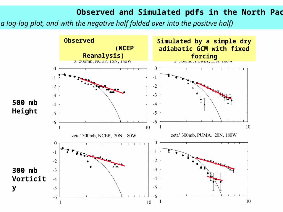
Observed and Simulated pdfs in the North Pacific

(On a log-log plot, and with the negative half folded over into the positive half)

500 mb Height

300 mbVorticity

Observed (NCEP Reanalysis)

Simulated by a simple dry adiabatic GCM with fixed forcing

Observed and Simulated pdfs in the North Pacific

(On a log-log plot, and with the negative half folded over into the positive half)

500 mb Height

300 mbVorticity

Observed (NCEP Reanalysis)

Simulated by a simple dry adiabatic GCM with fixed forcing

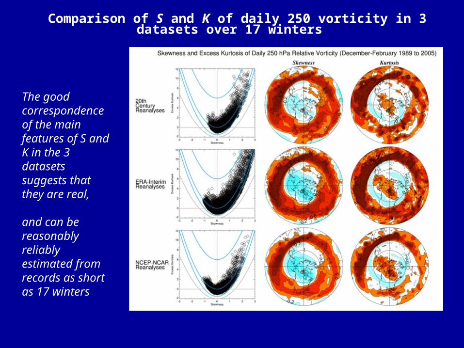
Comparison of S and K of daily 250 vorticity in 3 datasets over 17 winters

The good correspondence of the main features of S and K in the 3 datasets suggests that they are real,

and can be reasonably reliably estimated from records as short as 17 winters

S and K of daily anomalies computed over 115 winters (1891-2005) in the 20CR dataset

K-S plot Skewness S Kurtosis K

250 mb Vorticity

2m Air temperature

500 mbVertical Velocity (omega)

See Sardeshmukh and Sura (2009) for details

A generic “Stochastically Generated Skewed” (SGS) probability density function (PDF) suitable for describing non-Gaussian climate variability (Sardeshmukh and Sura J. Clim 2009)

λ > 0 b > 0

g > 0 or g < 0

E > 0

p(x) = 1N

(Ex+ g)2 + b2⎡⎣ ⎤⎦ − 1+

λE2

⎛⎝⎜

⎞⎠⎟ exp −

2λgE2b

arctanEx+ gb

⎛⎝⎜

⎞⎠⎟

⎡

⎣⎢

⎤

⎦⎥

If E → 0, then p(x) → a Gaussian PDF

Such a PDF has power-law tails, and its moments always satisfy K > (3/2) S2

Mean = < x > = 0 Lag Covariance = C(τ ) = σ 2 exp(−λτ )

Variance σ 2 = < x2 > = g2 + b2

2λ −E2 Power Spectrum = P(ω ) = 2σ 2λλ 2 +ω 2

Skewness S = < x3 >σ 3 =

2Egλ −E2( )σ

Kurtosis K = < x4 >σ 4 −3 =

32

λ −E2

λ −(3 / 2)E2

⎡

⎣⎢

⎤

⎦⎥ S

2 + 3E2

λ −(3 / 2)E2

⎡

⎣⎢

⎤

⎦⎥ ≥

32 S2

The parameters of this model (and of the PDF) can be estimated using the first four moments of x and its correlation scale. The model can then be run to generate Monte Carlo estimates of extreme statistics

dx

dt = − λ +

12E2⎛

⎝⎜⎞⎠⎟x + b η1 + (Ex+ g) η2 −

12Eg

If E → 0 , this is just the evolution equation for Gaussian "red noise"

This PDF arises naturally as the PDF of the simplest 1-D damped linear Markov process that is perturbed by Correlated Additive and Multiplicative white noise (“CAM noise”)

η1 and η2 are

Gaussian white noises

of unit amplitude.

Met. 101: The PDF of vertical velocity w strongly affects the PDF of precipitation

Mean Descent Mean Zero Mean Ascent

To a first approximation, the precipitation PDFhas the same shape as the shape of the w PDF for positive w

This is the basic reason why the PDFs of even seasonal mean precipitation are generally positively skewed, and are more skewed in drought-prone regions of mean descent

The shape of the w PDF strongly affects extreme precipitation risks

Sharply contrasting behavior of extreme w anomalies (and by implication, of extreme precipitation anomalies)

obtained in 107-day runs (equivalent to 105 100-day winters) of the Gaussian and non-Gaussian models

Blue curves: Time series of decadal maxima (i.e the largest daily anomaly in each decade = 1000 days = 10 100-day winters)

Orange curves: Time series of 99.5th decadal percentile (i.e. the 5th largest daily anomaly in each decade)

Non-Gaussian (S=1, K=5) Gaussian Gaussian (red) and non-Gaussian (black, S=1, K=5) PDFs with same mean and variance

PDFs of winter precipitation maxima, and their sampling uncertainties,

when the PDF of daily w is Gaussian or non-Gaussian

PDFs of daily w : Gaussian and non-Gaussian (S=1, K=5)

Thick curves: PDF of precipitation maxima in 105 winters when the daily w PDF is Gaussian or non-Gaussian (S=1, K=5)

Broad red and and grey bands : 90% sampling uncertainty if the PDF is estimated directly using the sample extreme values in 1000 100-winter segments of the 105-winter runs

Narrower dark grey band : 90% sampling uncertainty if the PDF is estimated indirectly using the sample S and K in 1000 100-winter segments of the 105-winter run

Summary

1. The PDFs of daily anomalies are significantly skewed and heavy-tailed. This fact has large implications both for the probabilities of extreme events and for estimations of those probabilities. Direct estimations, or estimations based on GEV distributions, become even more prone to sampling errors than in the Gaussian case.

2. We have demonstrated the relevance of a class of “stochastically generated skewed” (SGS) distributions for describing and investigating daily non-Gaussian atmospheric variability.

3. We have provided a physical basis for such SGS distributions as being distributions of simple damped linear Markov processes that are perturbed by Correlated Additive and Multiplicative white noise (“CAM noise”).

4. The parameters of the Markov model can be estimated from the first four statistical moments of a climate variable (mean, variance, skewness and kurtosis). The model can then be run to generate not only the appropriate SGS distribution, but also to estimate various sampling uncertainties in that distribution through extensive Monte Carlo integrations.

5. We have presented numerical evidence that the estimation of extreme-value distributions from century-long records of daily values can be more reliably accomplished indirectly using such a Markov model approach than through direct approaches.

PDFs of winter precipitation maxima, and their sampling uncertainties,

when the PDF of daily w is Gaussian or non-Gaussian

PDFs of daily w : Gaussian and non-Gaussian (S=1, K=5)

Thick curves: PDF of precipitation maxima in 105 winters when the daily w PDF is Gaussian or non-Gaussian (S=1, K=5)

Broad red and and grey bands : 90% sampling uncertainty if the PDF is estimated directly using the sample extreme values in 1000 100-winter segments of the 105-winter runs

Narrower dark grey band : 90% sampling uncertainty if the PDF is estimated indirectly using the sample S and K in 1000 100-winter segments of the 105-winter run

The SGS-distribution theory makes a simple prediction in this regard :

Under a climate shift , the PDF of retains the same general form

And if , then all increase,

and extreme risks become more extreme : even with respect to the shifted mean climate

Sardeshmukh, Compo, and Penland (2011)

x → X + x x

g + EX > g σ 2 , S2 , and K

Will extreme events become even more extreme if the mean climate shifts ?

Current Climate

g g2 +b2

E2

λ

+1−1

23

increases skewdecreases skew

Effect of a positive climate shift on PDF parameters

dx

dt = − λ +

12E2⎛

⎝⎜⎞⎠⎟x + b η1 + (Ex+ g) η2 −

12Eg

Shifted Climate

( X = 0.5 )

σ =1.1, S = 1.5, K = 7

σ =1, S = 1, K = 5

Chances in a decade : 1 10

Chances in a decade : 6 30