2장MATLAB 기초 - ::: AANCL - AeroAcoustics & Noise Control …aancl.snu.ac.kr/aancl/lecture/up_file/_1444008740_Matlab.pdf · 2017-06-16 · 2.1 MATLAB 환경 명령창-명령을입력하는창

2장 MATLAB 기초2장 MATLAB 기초

2.1 MATLAB 환경

2.2 배정

2.3 수학적 연산

2.4 내장함수의 사용

2 5 그래픽2.5 그래픽

2.6 다른 자원

2.1 MATLAB 환경경

명령창- 명령을 입력하는 창

그래프창>> (명령어 길잡이)>> 55 - 16

- 그래프를 나타내는 창

편집창

ans =39

>> ans + 11- M-파일을 편집하는 창

>> ans 11ans =

50

Applied Numerical MethodsApplied Numerical Methods

2.2 배정 (1/10)정

[스칼라]

>> a = 4

a =

4

>> A 6>> A = 6;

>> a =4, A=6; x= 1;

a =a

4

>> x

x =

1


2.2 배정 (2/10)정

[스칼라] 복소수

>> x = 2 + i*4

x =

2.0000 + 4.0000i

>> 2 j 4>> x = 2 + j*4

x =

2 0000 + 4 0000i2.0000 + 4.0000i


2.2 배정 (3/10)정

[스칼라] 포맷 형태

>> pi ans =

3.1416 >> format long (15자리 유효숫자) >> pi ans =

3.14159265358979 >> format short (소수점 이하4자리)>> pi ans =ans

3.1416


2.2 배정 (4/10)정

[배열, 벡터와 행렬]

>> a = [ 1 2 3 4 5]

a =

1 2 3 4 5

>> b = [2; 4; 6; 8; 10] 열벡터>> b = [2; 4; 6; 8; 10] 열벡터

b =

2

4

6

8

10


2.2 배정 (5/10)정


>> A = [1 2 3; 4, 5, 6; 7 8 9]

A =

1 2 3

4 5 64 5 6

7 8 9

>> who

Your variables are:

A a ans b x


2.2 배정 (6/10)정


>> whos

Name Size Bytes Class

A 3x3 72 double array

ba 1x5 40 double array

ans 1x1 8 double array

b 5 1 40 double arrab 5x1 40 double array

x 1x1 16 double array (complex)

Grand total is 21 elements using 176 bytesGrand total is 21 elements using 176 bytes


2.2 배정 (7/10)정


>> b(4) A =

ans =

8

>> A(2 3)

1 2 3

4 5 6

7 8 9

b =>> A(2,3)

ans =

6

2

4

6

8

>> E=zeros(2,3)

E =

10

0 0 0

0 0 0


2.2 배정 (8/10)정

[콜론 연산자]

>> t = 1:5

t =

1 2 3 4 5

>> 1 0 5 3>> t = 1:0.5:3

t =

1 0000 1 5000 2 0000 2 5000 3 00001.0000 1.5000 2.0000 2.5000 3.0000

>> t = 10: -1:5

t =

10 9 8 7 6 5


2.2 배정 (9/10)정

[콜론 연산자]

>> A(2,:)A =

ans =

4 5 6

>> t(2:4)

A =

1 2 3

4 5 6

7 8 9

t =>> t(2:4)

ans =

9 8 7

t =

10 9 8 7 6 5


2.2 배정 (10/10)정

[linspace와 logspace 함수 ]

>> linspace(0,1,6)

ans =

0 0.2000 0.4000 0.6000 0.8000 1.0000

>> logspace(-1,2,4)

ans =

0.1000 1.0000 10.0000 100.0000


2.3 수학적 연산 (1/7)

[계산순서]

지수계산 (^)

음부호 (-)음부호 (-)

곱셈과 나눗셈 (*, /)

왼쪽 나눗셈 (＼)

덧셈과 뺄셈 (+, -)


2.3 수학적 연산 (2/7)

>> 2*pi

ans =

6.2832

>> y=pi/4;

>> y^2 45>> y 2.45

ans =

0.5533

>> y=-4^2

y =

-16


2.3 수학적 연산 (3/7)

>> y=(-4)^2

y =

1616

>> x=2+4i

x =

2.0000 + 4.0000i

>> 3*x

ans =ans =

6.0000 +12.0000i

>> 1/x

ans =

0.1000 - 0.2000i


2.3 수학적 연산 (4/7)

>> x^2

ans = x =

2.0000 + 4.0000i

-12.0000 +16.0000i

>> x+y

ans =

y =

16

ans =

18.0000 + 4.0000i

>> a=[1 2 3];

>> b=[4 5 6]';

>> A=[1 2 3; 4 5 6; 7 8 9];


2.3 수학적 연산 (5/7)

>> a*A

ans =a =

1 2 3

30 36 42

>> A*b

ans =

b =

4

5

6ans =

32

77

A =

1 2 3

4 5 6

7 8 9

122

>> A*a

??? Error using ==> *

Inner matrix dimensions must agree.


2.3 수학적 연산 (6/7)

>> A*A

ans =A =

1 2 3

30 36 42

66 81 96

102 126 150

4 5 6

7 8 9

102 126 150

>> A/pi

ans =

0.3183 0.6366 0.9549

1.2732 1.5915 1.9099

2.2282 2.5465 2.8648


2.3 수학적 연산 (7/7)

>> A^2 행렬의 곱A =

1 2 3

ans =

30 36 42

66 81 96

4 5 6

7 8 9

66 81 96

102 126 150

>> A.^2 원소별 거듭제곱원 별 거듭제곱

ans =

1 4 9

16 25 36

49 64 81


2.4 내장함수의 사용 (1/9)장 용

Help 명령어를 사용하여 온라인 도움을 얻음

>> help log

Help 명령어를 사용하여 온라인 도움을 얻음

>> help log

LOG Natural logarithm.

LOG(X) is the natural logarithm of the elements of X.

Complex results are produced if X is not positive.

See also LOG2, LOG10, EXP, LOGM.

…



>> help elfun (모든 내장 함수를 볼 수 있음)

Elementary math functions.

Trigonometric.

sin Sinesin - Sine.

sinh - Hyperbolic sine.

asin - Inverse sine.

asinh - Inverse hyperbolic sine.

cos - Cosine.

…




Exponential.

exp - Exponential.

log Natural logarithmlog - Natural logarithm.

log10 - Common (base 10) logarithm.

…

sqrt - Square root.

…




Complex.

abs - Absolute value.

angle Phase angleangle - Phase angle.

complex - Construct complex data from real and imaginary parts.

…




Rounding and remainder.

fix - Round towards zero.

floor Round towards minus infinityfloor - Round towards minus infinity.

ceil - Round towards plus infinity.

round - Round towards nearest integer.g

mod - Modulus

(signed remainder after division).

rem - Remainder after division.

sign - Signum.



>> sin(pi/2)

ans =

11

>> exp(1)

ans =s

2.7183

>> abs(1+2i)

ans =

2.2361

>> fix(1 9) : FIX(X) rounds the elements of X to>> fix(1.9) : FIX(X) rounds the elements of X to

the nearest integers towards zero.

ans =


1


>> ceil(1.9)ans =

2

A =

1 2 32>> round(1.9)ans =

2

4 5 6

7 8 9

2>> rem(7,3) : remainder after divisionans =

11>> log(A)ans =

0 0 6931 1 09860 0.6931 1.09861.3863 1.6094 1.79181.9459 2.0794 2.1972



>> t=[0:2:20]'t =

022468810121414161820

( )>> length(t)ans =

11



>> g=9.81; m=68.1; cd=0.25;>> v=sqrt(g*m/cd)*tanh(sqrt(g*cd/m)*t)v =v

018.729233 111833.111842.076246.957549.421449.421450.617551.187151.456051.582351.6416


2.5 그래픽 (1/2)

그래프를 빠르고 편리하게 그릴 수 있음

>> plot(t,v)>> plot(t,v)

>> title('Plot of v versus t')

>> xlabel('Value of t')

>> ylabel('Value of v')

>> grid


2.5 그래픽 (2/2)

그래프를 빠르고 편리하게 그릴 수 있음

>> plot(t,v)>> plot(t,v)

>> title('Plot of v versus t')

>> xlabel('Value of t')

>> ylabel('Value of v')

>> grid

>> plot(t 'bo:')>> plot(t,v,'bo:')% blue dotted line

with circles on it (표 2.2 참조)


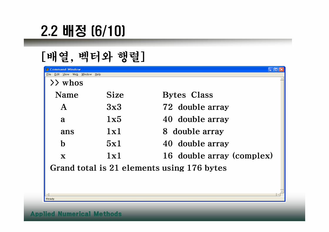
3장 MATLAB 프로그래밍3장 MATLAB 프로그래밍

3.1 M-파일

3 2 입력 출력3.2 입력-출력

3.3 구조 프로그래밍

3.4 내포화와 들여쓰기

3.5 M-파일로의 함수 전달

3.6 사례연구: 번지점프하는 사람의 속도

3장 MATLAB 프로그래밍장 밍

수학적 모델:

d 2vmcg

dtdv d−=

Euler법:

mdt

Euler법:

tddvvv i

ii Δ+=+1 dtii+1


3.1 M-파일 (1/5)

스크립트 파일- 일련의 MATLAB 명령어를 구성되어 저장된 M-파일이다.

%scriptdemo.m

g=9.81; m=68.1; cd=0.25; t=12;g 9.81; m 68.1; cd 0.25; t 12;

v=sqrt(g*m/cd)*tanh(sqrt(g*cd/m)*t)

>> scriptdemo

v =

50.6175


3.1 M-파일 (2/5)

함수 파일- function이라는 단어로 시작하는 M-파일이다.

function outvar = funcname(arglist)

%h l t%helpcomments

statements

outvar = value;여기서 outvar = 출력변수의 이름

funcname = 함수의 이름outvar value; funcname = 함수의 이름

arglist = 함수의 인수목록

helpcomments

= 사용자가 제공하는 함수에 관한 정보

statements

= value를 계산하여 그 값을

outvar에 배정하는 문장


예제 3.2 (1/3)

function v = freefallvel(t m cd)function v = freefallvel(t, m, cd)

%freefallvel: bungee velocity with second-order drag

%v=freefallvel(t,m,cd) computes the free-fall velocity

% of an object with second-order drag% of an object with second order drag

%input:

%t=time(s)

%m=mass(kg)%m mass(kg)

%cd=second order drag coefficient (kg/m)

%output:

%v=downward velocity (m/s)y ( / )

g=9.81; %accelearation of gravity

v=sqrt(g*m/cd)*tanh(sqrt(g*cd/m)*t);


예제 3.2 (2/3)

>> freefallvel(12, 68.1, 0.25)

…

>> freefallvel(12, 68.1, 0.25)

ans =

50.6175

>> freefallvel(8, 100, 0.25)

ans =

…

ans =

53.1878


예제 3.2 (3/3)

>> help freefallvel

freefallvel: bungee velocity with second-order drag

f f ll l(t d) t th f f ll l itv=freefallvel(t,m, cd) computes the free-fall velocity

of an object with second-order drag.

input:

…

d d l it ( / )v = downward velocity (m/s)


u1

슬라이드 7

u1 수정user, 12/3/2007

3.1 M-파일 (3/5)

- 함수 M-파일은 2개 이상의 결과를 반환할 수 있다.

예) 벡터의 평균과 표준편차의 계산예) 벡터의 평균과 표준편차의 계산

f ti [ td ] t t ( )function [mean, stdev] = stats(x)

n=length(x);

mean=sum(x)/n;

td t( (( ) ^2/( 1)))stdev=sqrt(sum((x-mean).^2/(n-1)));

>> y=[8 5 10 12 6 7.5 4];

>> [m,s] =stats (y)

m =m =

7.5000

S =

2 8137


2.8137

3.1 M-파일 (4/5)

부함수(subfunctions) - 함수가 다른 함수를 부를 수 있다. 이러한 함수는 M-파

일을 구분하여 작성할 수도 있고, 한 개의 M 파일에 포함시킬 수도 있다시킬 수도 있다.

function v= freefallsubfunc(t, m, cd)

v=vel(t, m, cd);

d

주함수

end

function v=vel(t, m, cd)

g=9.81;

( / d) h( ( d/ ) )부함수

v=sqrt(g*m/cd)*tanh(sqrt(g*cd/m)*t);

end

부함수


3.1 M-파일 (5/5)

>> freefallsubfunc (12, 68.1, 0.25)

ans =

50.6175

>> vel (12, 68.1, 0.25), ,

??? Undefined command/function ‘vel’.


3.2 입력-출력 (1/4)

input 함수- 사용자로 하여금 명령창에서 직접 입력하도록 한다.

m = input ('Mass (kg): ')

name = input ('Enter your name: ' 's')name input ( Enter your name: , s )

%문자열을 받는 경우


3.2 입력-출력 (2/4)

disp 함수- 어떤 값을 손쉽게 나타낸다.

disp(' ')

disp('Velocity (m/s): ')disp( Velocity (m/s): )

%문자열을 나타내는 경우


3.2 입력-출력 (3/4)

fprintf 함수- 정보를 표현할 때 추가적인 제어를 제공한다.

fprintf ('format', x, …)

%포맷코드와 제어코드를 넣어서 나타내는 경우%포맷코드와 제어코드를 넣어서 나타내는 경우

>> fprintf(‘The velocity is %8.4f m/s\n’ velocity)

The velocity is 50 6175 m/sThe velocity is 50.6175 m/s


3.2 입력-출력 (4/4)

포맷 코드 설 명

%d

%e

정수 포맷

e를 사용하는 과학 포맷

%E

%f

%

E를 사용하는 과학 포맷

소수 포맷

% 나 %f 중 간단한 포맷%g %e나 %f 중 간단한 포맷

제어 코드 설 명

₩n

₩t

새로운 줄로 시작

탭


예제 3.3 (1/3)

function freefalli

% freefalli: interactive bunge velocity

% f f lli i i i f h% freefalli interactive computation of the

% free-fall velocity of an object

% with second-order drag.g

g=9.81; % acceleration of gravity

m=input('Mass(kg):');

d i t('D ag C ffi i t(kg/ ):');cd=input('Drag Coefficient(kg/m):');


예제 3.3 (2/3)

t=input('Time(s):');

disp(' ')disp(' ')

disp('Velocity (m/s):')

disp(sqrt(g*m/cd)*tanh(sqrt(g*cd/m)*t))

minusvelocity= -sqrt(g*m/cd)* tanh(sqrt(g*cd/m)*t);

fprintf('The velocity is %8.4f m/s\n', minusvelocity)

i t ('E t : ' ' ');name = input ('Enter your name: ', 's');

disp('Your name is'); disp(name)


예제 3.3 (3/3)

명령창에서 다음과 같이 입력한다.

>> freefalli

Mass (kg): 68.1

Drag coefficient (kg/m): 0.25

Ti ( ) 12Time (s): 12

Velocity (m/s):

50.617550.6 75

The velocity is -50.6175 m/s

Enter your name: Kim

Your name is

Kim


3.3 구조 프로그래밍 (1/12)밍

명령을 연속적으로 수행하지 않는 것을

허용하는 구문

판정 ( 는 선택)- 판정 (또는 선택): 판정에 기초를 둔 흐름의 분기점이다.

- 루프 (또는 반복): 반복을 허용하는 흐름의 루프이다.

판정

[if 구조] if condition

statements

endend



function grader(grade)

if grade >= 60

disp('passing grade:')

>> grader(95.6)

passing grade:

95.6000disp( passing grade: )

disp(grade)

end

95.6000



[에러 함수]

error ( msg)

에러 함수

f ti f t t( ) >> errortest(10)function f = errortest(x)

if x==0,

error(' zero value encountered'),

d

>> errortest(10)

ans =

0.1000

>> errortest(0)end

f=1/x;

>> errortest(0)

??? Error using ==> errortest

zero value encountered


u2

슬라이드 20

u2 수정user, 12/3/2007


[논리조건][논리조건]

value1 relation value2

~ (Not) - 논리적 부정을 나타낼 때 사용한다.

& (And) - 두 식에서 논리적 곱을 나타낼 때 사용한다.

| (Or) - 두 식에서 논리적 합을 나타낼 때 사용한다.



<복잡한 논리식의 단계별 계산>


<복잡한 논리식의 단계별 계산>


[if … else 구조] [if … elseif 구조]

if condition if condition1

[if … else 구조] [if … elseif 구조]

statements1

else

statements2

statements1

elseif condition2

statements2statements2

end

statements2

…

else

statementselse

end


예제 3.4 (1/3)

……

풀이) 내장함수인 sign 함수의 기능을 알아보자.

>> sign(25.6)

ans =

1

>> sign(-0.776)

ans =ans =

-1

>> sign(0)

ans =

0


예제 3.4 (2/3)

function sgn = mysign(x)

% i ( ) t 1 1 d 0 f iti ti d% mysign(x) returns 1, -1, and 0 for positive, negative, and zero values, respectively.

%

if x > 0

sgn = 1;

elseif x < 0

sgn = -1;

else

sgn = 0;sgn 0;

end


예제 3.4 (3/3)

명령창에서 다음과 같이 확인할 수 있다.

>> mysign(25.6)ans =

1

>> mysign(-0.776)ans =

1-1

>> mysign(0)ansans =

0



루프

[for … end 구조]

for index = start:step:finish

statements

end


예제 3.5 (1/3)

풀이) factorial 함수와 같은 기능을 갖도록 for 루프를 사용하여풀이) factorial 함수와 같은 기능을 갖도록 for 루프를 사용하여

프로그램을 작성한다.

>> factorial(5)

ans =a s

120


예제 3.5 (2/3)

function fout = factor(n)

% computes the product of all integers from 1 to n.

%

x = 1;x 1;

for i=1:n

x = x * i;

end

fout = x;

endend


예제 3.5 (3/3)

명령창에서 다음과 같이 확인할 수 있다.

>> factor(5)

ans =

120



[벡터화]

i = 0;

for t = 0:0.02:5

[벡터화]

i = i + 1;

y(i) = cos(t);

end

t = 0:0.02:5;

( )y = cos(t);


u3

슬라이드 31

u3 수정user, 12/3/2007


[while 구조]

while condition

statements

endend


3.3 구조 프로그래밍 (10/12)밍

>> x = 8

x =x =

8

>> while x > 0

x = x - 3;

disp(x)

end

5

22

-1


3.3 구조 프로그래밍 (11/12)밍

[while … break 구조]

while (1)

[ 구 ]

statements

if condition, break, end

statementsstatements

end


3.3 구조 프로그래밍 (12/12)밍

>> 0 24>> x= 0.24x =

0.2400>> while(1)>> w e( )

x = x - 0.05if x<0, break, end %후기점검 루프

endx =

0.1900x =

0.14000.1400x =

0.0900x =

0 04000.0400x =

-0.0100


3.4 내포화와 들여쓰기

내포화- 다른 구조 안에 구조를 배치하는 것이다다른 구조 안에 구조를 배치하는 것이다.


예제 3.6 (1/3)

cbxaxxf ++= 2)(

bb 42±a

acbbx2

42 −±−=

a2


예제 3.6 (2/3)

function quadroots(a, b, c)

f d i i% quadroots : roots of a quadratic equation

% quadroots(a, b, c) : real and complex roots

% of quadratic equation% of quadratic equation

% input:

% a = second-order coefficient% a second order coefficient

% b = first-order coefficient

% c = zero-order coefficient

% output:

% r1: real part of first root


예제 3.6 (2/3)

% i1: imaginary part of first root

% r2: real part of second root

% i2: imaginary part of second root

if a == 0if a 0

%special cases

if b~= 0 %single root

/r1=-c/b

else %trivial root

error(' Trivial solution. Try again! ')y g

end


예제 3.6 (2/3)

else

%quadratic formula

d=b^2 – 4*a*c; %discriminant

if d>=0if d>=0

% real roots

r1 = (-b+sqrt(d))/(2*a)

r2 = (-b-sqrt(d))/(2*a)

else


예제 3.6 (2/3)

% l t%complex roots

r1 = -b/(2*a)

i1 = sqrt(abs(d))/(2*a)

r2=r1

i2=-i1

endend

end


예제 3.6 (3/3)

>> quadroots(1 1 1)>> quadroots(1,1,1)

r1 =

-0.5000

i1 =

0.8660

r2 =

-0.5000

i2 =i2 =

-0.8660


예제 3.6 (3/3)

>> quadroots(1 5 1)>> quadroots(1,5,1)

r1 =

-0.2087

r2 =

-4.7913

( )>> quadroots(0,0,0)

??? Error using ==> quadroots

Trivial solution Try again!Trivial solution. Try again!


3.5 M-파일로의 함수 전달 (1/7)

무명 함수- M-파일을 만들지 않고 간단한 함수를 생성할 수 있게 한다.

명령창에서 다음과 같은 구문을 사용한다.

fhandle = @(arglist) expression

>> outvar =feval('cos',pi/6)>> fl = @(x,y) x^2 + y^2;

>> fl (3 4)>> fl (3,4)

ans =

25


u8

슬라이드 44

u8 수정user, 12/4/2007


inline 함수- Matlab 7 이전에서 무명함수와 같은 역할 수행.

funcname = inline('expression',`'var1' , 'var2' ,…) u c a e e( e p ess o , va , va , )

( )>> f1 =inline('x^2 + y^2', 'x', 'y')

f1 =

inline function:inline function

f1(x,y) = x^2 + y^2

>> f1(3,4)

ans =

25



function 함수- 다른 함수에 작동하는 함수.

예 ) fplot (fun lims)예 ) fplot (fun, lims)

>> vel= @(t)…

sqrt(9.81*68.1/0.25)*

h( (9 81 0 25/68 1) )tanh(sqrt(9.81*0.25/68.1)*t);

>> fplot(vel, [0 12])


u9

슬라이드 46

u9 수정user, 12/4/2007

예제 3.7예제

( ) tanhd d

gm gmv t tC C

⎛ ⎞= ⎜ ⎟⎜ ⎟

⎝ ⎠d dC C⎝ ⎠

풀이) t=0에서 t=12까지의 범위에서 함수 값을 그래프로 그릴 수있다.있다.

>> t=linspace(0 12);>> t=linspace(0, 12);

>> v= sqrt(9.81*68.1/0.25)*tanh(sqrt(9.81*0.25/68.1)*t);

>> mean(v)

ans =

36.0870



function favg = funcavg(f, a, b, n)% input:% f = function to be evaluated% a= lower bound of rangeg% b= upper bound of range% n= number of intervals% output:% output% favg = average value of functionx = linspace(a,b,n);y=f(x);y=f(x);favg=mean(y);



>> vel= @(t)…

sqrt(9.81*68.1/0.25)*tanh(sqrt(9.81*0.25/68.1)*t);

>> funcavg(vel, 0, 12, 60)

ans =

36.0127

>> funcavg(@sin, 0, 2*pi, 180)

ans =ans

-6.3001e-017



매개변수의 전달- 매개변수에 새로운 값을 취할 때 편리함.

- function 함수의 마지막 입력인수에 varargin 추가함.수의 마지막 력 수에 g 추가

[ funcavg의 수정 ]

function favg = funcavg (f, a, b, n, varargin)

x = linspace(a b n);x linspace(a,b,n);

y = f(x, varargin{:});

favg = mean(y)



>> vel= @(t, m, cd) sqrt(9.81*m/cd)*tanh(sqrt(9.81*cd/m)*t);

>> funcavg(vel, 0, 12, 60, 68.1, 0.25) %m=68.1, cd=0.25

ans =

36 012736.0127

>> funcavg(vel, 0, 12, 60, 100, 0.28) %m=100, cd=0.28

ans =

38.9345


3.6 사례연구: 번지점프하는 사람의 속도 (1/4)

수학적 모델:

cdv 2vmc

gdtdv d−=

Euler법:Euler법:

tdv

vv iii Δ+=+1 dtii+1


3.6 MATLAB M-파일: 번지점프하는 사람의 속도 (2/4)

function vend = velocity1(dt, ti, tf, vi)

% velocity1: Euler solution for bungee velocity

% vend = velocity1(dt, ti, tf, vi)

% Euler method solution of bunge% s b g

% jumper velocity

% inputs:

% dt = time step (s)% dt = time step (s)

% ti = initial time (s)

% tf = final time (s)

% i i i i l l f d d i bl ( / )% vi = initial value of dependent variable (m/s)



% output:

% vend = velocity at tf (m/s)% vend = velocity at tf (m/s)

t = ti;

v = vi;

n = (tf - ti)/dt;

for i=1:n

dvdt= deriv(v);

v = v + dvdt *dt;

t = t + dt;

endend

vend = v;

end



function dv = deriv( v)( )

dv = 9.81 – (0.25 / 68.1)*v^2;

end



>> l it 1(0 5 0 12 0) 간격 번을 계산>> velocity1(0.5, 0, 12, 0) %0.5초 간격, 24번을 계산

ans =

50.9259

>> velocity1(0.01, 0, 12, 0) %0.01초 간격, 1,200번을 계산

ans =

50 623950.6239

>> velocity1(0.001, 0, 12, 0) %0.001초 간격, 12,000번을 계산

ans =

50.6181


Documents

2장MATLAB 기초 - ::: AANCL - AeroAcoustics & Noise Control …aancl.snu.ac.kr/aancl/lecture/up_file/_1444008740_Matlab.pdf · 2017-06-16 · 2.1 MATLAB 환경 명령창-명령을입력하는창