2D Projective Geometry

CS 600.361/600.461

Instructor: Greg Hager

(Adapted from slides by N. Padoy, S. Seitz, K. Grauman and others)

Outline •  Linear least squares •  2D affine alignment •  Image warping •  Perspective alignment •  Direct linear algorithm (DLT)

2

Reminders

Reminder – Corner detection/matching

€

M =∑IxIx IxIyIxIy IyIy

#

$ %

&

' (

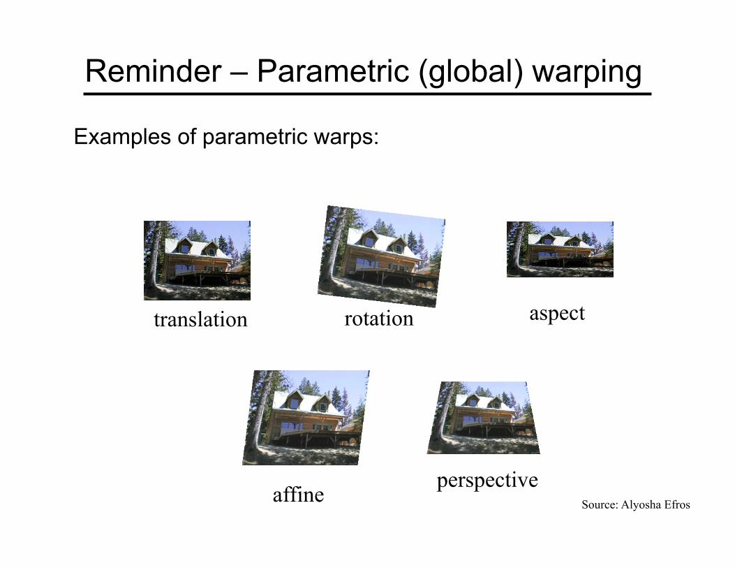
Reminder – Parametric (global) warping

Examples of parametric warps:

translation rotation aspect

affine perspective

Source: Alyosha Efros

Reminder – 2D Affine Transformations

Affine transformations are combinations of … •  Linear transformations, and •  Translations

Parallel lines remain parallel

⎥⎥⎥

⎦

⎤

⎢⎢⎢

⎣

⎡

⎥⎥⎥

⎦

⎤

⎢⎢⎢

⎣

⎡

=

⎥⎥⎥

⎦

⎤

⎢⎢⎢

⎣

⎡

wyx

fedcba

wyx

100'''

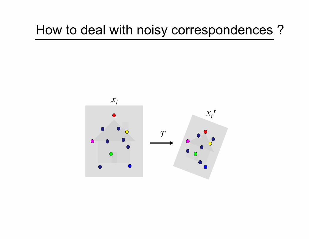
Reminder – Alignment problem

We have previously considered how to fit a model to image evidence •  e.g., a line to edge points

In alignment, we will fit the parameters of some transformation according to a set of matching feature pairs (“correspondences”).

T

xi

xi '

Reminder – Fitting an affine transformation

•  Assuming we know the correspondences, how do we get the transformation?

),( ii yx ʹ′ʹ′),( ii yx

⎥⎦

⎤⎢⎣

⎡+⎥⎦

⎤⎢⎣

⎡⎥⎦

⎤⎢⎣

⎡=⎥⎦

⎤⎢⎣

⎡ʹ′

ʹ′

2

1

43

21

ttyxmmmm

yx

i

i

i

i

Reminder – Fitting an affine transformation

⎥⎥⎥⎥

⎦

⎤

⎢⎢⎢⎢

⎣

⎡

ʹ′

ʹ′=

⎥⎥⎥⎥⎥⎥⎥⎥

⎦

⎤

⎢⎢⎢⎢⎢⎢⎢⎢

⎣

⎡

⎥⎥⎥⎥

⎦

⎤

⎢⎢⎢⎢

⎣

⎡

i

i

ii

ii

yx

ttmmmm

yxyx

2

1

4

3

2

1

10000100

•  Least square minimization:

2minBAx−

Reminder – Singular Value Decomposition

Given any m×n real matrix A, algorithm to find matrices U, V, and D such that

A = U D VT U is m×m and orthogonal D is m×n and diagonal V is n×n and orthogonal

€

A

"

#

$ $ $ $ $ $

%

&

' ' ' ' ' '

= U

"

#

$ $ $ $ $ $

%

&

' ' ' ' ' '

d1 0 00 00 0 dp0 0 00 0 0

"

#

$ $ $ $ $ $

%

&

' ' ' ' ' '

V

"

#

$ $ $

%

&

' ' '

T

€

d1 ≥ d2 ≥ ≥ dp ≥ 0 for p=min(m,n)

Linear least squares

(Board)

LLS - Method 1

Linear least-squares solution to an overdetermined full-rank set of linear equations

(Picture from Hartley’s book, appendix 5)

LLS – Method 2

(Picture from Hartley’s book, appendix 5)

Note: if A is not full rank, this is in general a different solution than the one from method 1

Linear least-squares solution to an overdetermined full-rank set of linear equations

Matlab: check the functions svd, pinv, mldivide

LLS – Method 3

Linear least-squares solution to a homogeneous system of linear equations

(Picture from Hartley’s book, appendix 5)

RANSAC for affine alignment

How to deal with noisy correspondences ?

xi

xi '

T

Reminder: RANSAC for line fitting

Repeat N times: •  Draw s points uniformly at random •  Fit line to these s points •  Find inliers to this line among the remaining points (i.e., points

whose distance from the line is less than t) •  If there are d or more inliers, accept the line and refit using all

inliers

Lana Lazebnik

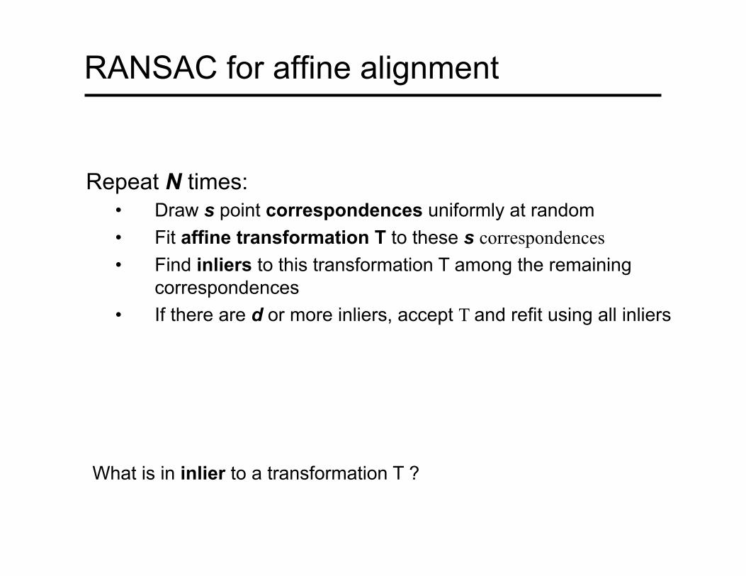
RANSAC for affine alignment

Repeat N times: •  Draw s point correspondences uniformly at random •  Fit affine transformation T to these s correspondences •  Find inliers to this transformation T among the remaining

correspondences •  If there are d or more inliers, accept T and refit using all inliers

What is in inlier to a transformation T ?

Inliers to a transformation T

•  Two of several possibilities •  Using asymmetric transfer error

(x,x’) such that ||x’-Tx|| below a threshold t •  Using symmetric transfer error

(x,x’) such that ||x’-Tx||+||x-inv(T)x’|| below t

T

T

RANSAC example: Translation

Putative matches

Source: Rick Szeliski

RANSAC example: Translation

Select one match, count inliers

RANSAC example: Translation

Select one match, count inliers

RANSAC example: Translation

Find “average” translation vector

Note

We are not fully done yet…

•  How do we correctly warp (or unwarp) an image, per pixel, knowing T ?

•  What about the case of 2D perspective transformations ?

T

Is this an affine transformation ?

Image warping

Image warping

Given a coordinate transform and a source image f(x,y), how do we compute a transformed image g(x’,y’) = f(T(x,y))?

x x’

T(x,y)

f(x,y) g(x’,y’)

y y’

Slide from Alyosha Efros, CMU

f(x,y) g(x’,y’)

Forward warping

Send each pixel f(x,y) to its corresponding location (x’,y’) = T(x,y) in the second image

x x’

T(x,y)

Q: what if pixel lands “between” two pixels?

y y’

Slide from Alyosha Efros, CMU

f(x,y) g(x’,y’)

Forward warping

Send each pixel f(x,y) to its corresponding location (x’,y’) = T(x,y) in the second image

x x’

T(x,y)

Q: what if pixel lands “between” two pixels?

y y’

A: distribute color among neighboring pixels (x’,y’) –  Known as “splatting”

Slide from Alyosha Efros, CMU

f(x,y) g(x’,y’) x y

Inverse warping

Get each pixel g(x’,y’) from its corresponding location (x,y) = T-1(x’,y’) in the first image

x x’

Q: what if pixel comes from “between” two pixels?

y’ T-1(x,y)

Slide from Alyosha Efros, CMU

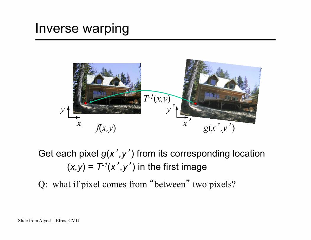
f(x,y) g(x’,y’) x y

Inverse warping

Get each pixel g(x’,y’) from its corresponding location (x,y) = T-1(x’,y’) in the first image

x x’

T-1(x,y)

Q: what if pixel comes from “between” two pixels?

y’

A: Interpolate color value from neighbors –  nearest neighbor, bilinear…

Slide from Alyosha Efros, CMU >> help interp2!

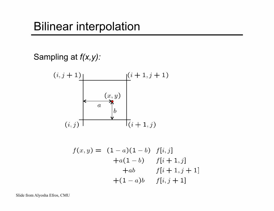
Bilinear interpolation

Sampling at f(x,y):

Slide from Alyosha Efros, CMU

2D projective geometry

Projective geometry

•  2D projective geometry •  Points on a plane (projective plane ) are represented in

homogeneous coordinates

•  Objective: study projective transformations and their invariants

•  Definition: a projective transformation h is an invertible mapping from to that preserves collinearity between points (x1, x2, x3 on same line => h(x1), h(x2),h(x3) on same line)

•  projective transformation = homography = collineation

P2

€

xyw

"

#

$ $ $

%

&

' ' '

P2 P2

Homography

Theorem A mapping if a projective transformation if and on if

there exists an invertible 3x3 matrix H such that for any point x represented in homogeneous coordinates, h(x)=Hx

⎥⎥

⎦

⎤

⎢⎢

⎣

⎡

⎥⎥

⎦

⎤

⎢⎢

⎣

⎡=

⎥⎥

⎦

⎤

⎢⎢

⎣

⎡

wyx

ihgfedcba

wyx

'''

h : P2 � P2

x’=h(x) x H

Note: equation is up to a scale factor

Reminder – 2D Affine Transformations

Affine transformations are combinations of … •  Linear transformations, and •  Translations

Parallel lines remain parallel

⎥⎥⎥

⎦

⎤

⎢⎢⎢

⎣

⎡

⎥⎥⎥

⎦

⎤

⎢⎢⎢

⎣

⎡

=

⎥⎥⎥

⎦

⎤

⎢⎢⎢

⎣

⎡

wyx

fedcba

wyx

100'''

2D Projective Transformations

Parallel lines do not necessarily remain parallel

⎥⎥

⎦

⎤

⎢⎢

⎣

⎡

⎥⎥

⎦

⎤

⎢⎢

⎣

⎡=

⎥⎥

⎦

⎤

⎢⎢

⎣

⎡

wyx

ihgfedcba

wyx

'''

Image warping with homographies

image plane in front image plane below black area where no pixel maps to

Source: Steve Seitz

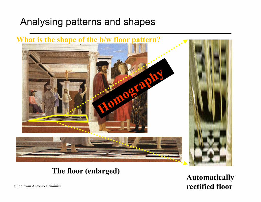
Analysing patterns and shapes

Automatically rectified floor

The floor (enlarged)

What is the shape of the b/w floor pattern?

Slide from Antonio Criminisi

From Martin Kemp The Science of Art (manual reconstruction)

Aut

omat

ic r

ectif

icat

ion

Analysing patterns and shapes

Slide from Antonio Criminisi

Automatically rectified floor

St. Lucy Altarpiece, D. Veneziano

Analysing patterns and shapes

What is the (complicated) shape of the floor pattern?

Slide from Criminisi

From Martin Kemp, The Science of Art (manual reconstruction)

Automatic rectification

Analysing patterns and shapes

Slide from Criminisi

Image rectification

p p’

How do we compute H ?

H

Solving for homographies

•  Up to scale. So, there are 8 degrees of freedom (DoF). •  Set up a system of linear equations:

Ah = 0 where vector of unknowns h = [h1,h2,h3,h4,h5,h6,h7,h8,h9]T

•  Need at least 8 eqs, but the more the better… •  Solve using least-squares

€

x'y'w'

"

#

$ $ $

%

&

' ' '

=

h1 h2 h3h4 h5 h6h7 h8 h9

"

#

$ $ $

%

&

' ' '

xyw

"

#

$ $ $

%

&

' ' '

p’ = Hp

(BOARD)

Summary: DLT algorithm

44

Objective Given n≥4 2D to 2D point correspondences {xi↔xi’}, determine the 2D homography matrix H such that xi’=Hxi

Algorithm (i)  For each correspondence xi ↔xi’ compute Ai. Usually only

two first rows needed. (ii)  Assemble n 2x9 matrices Ai into a single 2nx9 matrix A (iii)  Obtain SVD of A. Solution for h is last column of V (iv)  Determine H from h

€

0 0 0 −wi ' xi −wi ' yi −wi 'wi yi ' xi yi ' yi yi 'wi

wi ' xi wi ' yi wi 'wi 0 0 0 −xi ' xi −xi ' yi −xi 'wi

−yi ' xi −yi ' yi −yi 'wi xi ' xi xi ' yi xi 'wi 0 0 0

#

$

% % %

&

'

( ( (

€

Xi = xi yi wi[ ]T

€

Xi '= xi ' yi ' wi '[ ]T

Conclusion

•  Today •  Affine alignment •  RANSAC in presence of outliers •  Image warping •  Homography

•  Next time

•  More on homography estimation •  Mosaicing •  More projective geometry