290 IEEE TRANSACTIONS ON PATTERN ANALYSIS …jwp2128/Papers/BroderickMackeyetal2015.pdf · Combinatorial Clustering and the Beta Negative Binomial Process ... the NBP, and demonstrate

Combinatorial Clustering and the BetaNegative Binomial Process

Tamara Broderick, Lester Mackey, John Paisley, and Michael I. Jordan

Abstract—We develop a Bayesian nonparametric approach to a general family of latent class problems in which individuals can

belong simultaneously to multiple classes and where each class can be exhibited multiple times by an individual. We introduce a

combinatorial stochastic process known as the negative binomial process (NBP) as an infinite-dimensional prior appropriate for such

problems. We show that the NBP is conjugate to the beta process, and we characterize the posterior distribution under the beta-

negative binomial process (BNBP) and hierarchical models based on the BNBP (the HBNBP). We study the asymptotic properties of

the BNBP and develop a three-parameter extension of the BNBP that exhibits power-law behavior. We derive MCMC algorithms for

posterior inference under the HBNBP, and we present experiments using these algorithms in the domains of image segmentation,

object recognition, and document analysis.

Index Terms—Beta process, admixture, mixed membership, Bayesian, nonparametric, integer latent feature model

Ç

1 INTRODUCTION

IN traditional clustering problems the goal is to induce aset of latent classes and to assign each data point to one

and only one class. This problem has been approachedwithin a model-based framework via the use of finite mix-ture models, where the mixture components characterizethe distributions associated with the classes, and the mixingproportions capture the mutual exclusivity of the classes[10], [26]. In many domains in which the notion of latentclasses is natural, however, it is unrealistic to assign eachindividual to a single class. For example, in genetics, whileit may be reasonable to assume the existence of underlyingancestral populations that define distributions on observedalleles, each individual in an existing population is likely tobe a blend of the patterns associated with the ancestral pop-ulations. Such a genetic blend is known as an admixture [35].A significant literature on model-based approaches toadmixture has arisen in recent years [1], [7], [35], with appli-cations to a wide variety of domains in genetics and beyond,including document modeling and image analysis.1

Model-based approaches to admixture are generally builton the foundation of mixture modeling. The basic idea is to

treat each individual as a collection of data, with anexchangeability assumption imposed for the data within anindividual but not between individuals. For example, in thegenetics domain the intra-individual data might be a set ofgenetic markers, with marker probabilities varying acrossancestral populations. In the document domain the intra-individual data might be the set of words in a given docu-ment, with each document (the individual) obtained as ablend across a set of underlying “topics” that encode proba-bilities for the words. In the image domain, the intra-indi-vidual data might be visual characteristics like edges, hue,and location extracted from image patches. Each image isthen a blend of object classes (e.g., grass, sky, or car), eachdefining a distinct distribution over visual characteristics. Ingeneral, this blending is achieved by making use of theprobabilistic structure of a finite mixture but using a differ-ent sampling pattern. In particular, mixing proportions aretreated as random effects that are drawn once per individ-ual, and the data associated with that individual areobtained by repeated draws from a mixture model havingthat fixed set of mixing proportions. The overall model is ahierarchical model, in which mixture components areshared among individuals and mixing proportions aretreated as random effects.

Although the literature has focused on using finite mix-ture models in this context, there has also been a growingliterature on Bayesian nonparametric approaches to admix-ture models, notably the hierarchical Dirichlet process (HDP)[42], where the number of shared mixture components isinfinite. Our focus in the current paper is also on nonpara-metric methods, given the open-ended nature of the inferen-tial objects with which real-world admixture modeling isgenerally concerned.

Although viewing an admixture as a set of repeateddraws from a mixture model is natural in many situations,it is also natural to take a different perspective, akin tolatent trait modeling, in which the individual (e.g., a docu-ment or a genotype) is characterized by the set of “traits”

1. While we refer to such models generically as “admixture mod-els,” we note that they are also often referred to as topic models or mixedmembership models.

� T. Broderick and M.I. Jordan are with the Department of Statistics and theDepartment of Electrical Engineering and Computer Sciences, Universityof California, Berkeley, CA 94705.

� L. Mackey is with the Department of Statistics, Stanford University,Stanford, CA 94305.

� J. Paisley is with the Department of Electrical Engineering at ColumbiaUniversity, New York, NY 10027.

Manuscript received 15 Sept. 2012; revised 27 Nov. 2013; accepted 17 Feb.2014. Date of publication 17 Apr. 2014; date of current version 14 Jan. 2015Recommended for acceptance by R.P. Adams, E. Fox, E. Sudderth, and Y.W. Teh.For information on obtaining reprints of this article, please send e-mail to:[email protected], and reference the Digital Object Identifier below.Digital Object Identifier no. 10.1109/TPAMI.2014.2318721

290 IEEE TRANSACTIONS ON PATTERN ANALYSIS AND MACHINE INTELLIGENCE, VOL. 37, NO. 2, FEBRUARY 2015

0162-8828� 2014 IEEE. Personal use is permitted, but republication/redistribution requires IEEE permission.See http://www.ieee.org/publications_standards/publications/rights/index.html for more information.

or “features” that it possesses, and where there is noassumption of mutual exclusivity. Here the focus is on theindividual and not on the “data” associated with an indi-vidual. Indeed, under the exchangeability assumptionalluded to above it is natural to reduce the repeated drawsfrom a mixture model to the counts of the numbers oftimes that each mixture component is selected, and wemay wish to model these counts directly. We may furtherwish to consider hierarchical models in which there is alinkage among the counts for different individuals.

This idea has been made explicit in a recent line of workbased on the beta process. Originally developed for survivalanalysis, where an integrated form of the beta process wasused as a model for random hazard functions [16], morerecently it has been observed that the beta process also pro-vides a natural framework for latent feature modeling [44].In particular, as we discuss in detail in Section 2, a drawfrom the beta process yields an infinite collection of coin-tossing probabilities. Tossing these coins—a draw from aBernoulli process—one obtains a set of binary features thatcan be viewed as a description of an admixed individual. Akey advantage of this approach is the conjugacy betweenthe beta and Bernoulli processes: this property allows fortractable inference, despite the countable infinitude of coin-tossing probabilities. A limitation of this approach, how-ever, is its restriction to binary features; indeed, one of thevirtues of the mixture-model-based approach is that a givenmixture component can be selected more than once, withthe total number of selections being random.

We develop a model for admixture that meets all of thedesiderata outlined thus far. Unlike the Bernoulli processlikelihood, our featural model allows each feature to beexhibited any non-negative integer number of times by anindividual. Unlike admixture models based on the HDP,our model cohesively includes a random total number offeatures (e.g., words or traits) per individual (e.g., a docu-ment or genotype).

As inspiration, we note that in the setting of classical ran-dom variables, beta-Bernoulli conjugacy is not the onlyform of conjugacy involving the beta distribution—the neg-ative binomial distribution is also conjugate to the beta.Anticipating the value of conjugacy in the setting of non-parametric models, we define and develop a stochastic pro-cess analogue of the negative binomial distribution, whichwe refer to as the negative binomial process (NBP),2 and pro-vide a rigorous proof of its conjugacy to the beta process.We use this process as part of a new model—the hierarchicalbeta negative binomial process (HBNBP)—based on the NBPand the hierarchical beta process [44]. Our theoretical andexperimental development focus on the usefulness of theHBNBP in the admixture setting, where flexible modelingof feature totals can lead to improved inferential accuracy(see Fig. 3a and the surrounding discussion). However, theutility of the HBNBP is not limited to the admixture settingand should extend readily to the modeling of latent factorsand the identification of more general latent features. More-over, the negative binomial component of our model offers

additional flexibility in the form of a new parameterunavailable in either the Bernoulli or multinomial likeli-hoods traditionally explored in Bayesian nonparametrics.

The remainder of the paper is organized as follows. InSection 2 we present the framework of completely randommeasures (CRMs) that provides the formal underpinningsfor our work. We discuss the Bernoulli process, introducethe NBP, and demonstrate the conjugacy of both to the betaprocess in Section 3. Section 4 focuses on the problem ofmodeling admixture and on general hierarchical modelingbased on the negative binomial process. Sections 5 and 6 aredevoted to a study of the asymptotic behavior of the NBPwith a beta process prior, which we call the beta-negativebinomial process (BNBP). We describe algorithms for poste-rior inference in Section 7. Finally, we present experimentalresults. First, we use the BNBP to define a generative modelfor summaries of terrorist incidents with the goal of identi-fying the perpetrator of a given terrorist attack in Section 8.Second, we demonstrate the utility of a finite approximationto the BNBP in the domain of automatic image segmenta-tion in Section 9. Section 10 presents our conclusions.

2 COMPLETELY RANDOM MEASURES

In this section we review the notion of a completely randommeasure, a general construction that yields random meas-ures that are closely tied to classical constructions involvingsets of independent random variables. We present CRM-based constructions of several of the stochastic processesused in Bayesian nonparametrics, including the beta pro-cess, gamma process, and Dirichlet process (DP). In the fol-lowing section we build on the foundations presented hereto consider additional stochastic processes.

Consider a probability space ðC;F ;PÞ. A random measureis a random element m such that mðAÞ is a non-negative ran-dom variable for any A in the sigma algebra F . A completelyrandom measure m is a random measure such that, for anydisjoint, measurable sets A;A0 2 F , we have that mðAÞ andmðA0Þ are independent random variables [19]. Completelyrandom measures can be shown to be composed of at mostthree components:

1) A deterministic measure. For deterministic mdet, it istrivially the case that mdetðAÞ and mdetðA0Þ are inde-pendent for disjoint A;A0.

2) A set of fixed atoms. Let ðu1; . . . ; uLÞ 2 CL be a collec-tion of deterministic locations, and let ðh1; . . . ; hLÞ 2RL

þ be a collection of independent random weightsfor the atoms. The collection may be countablyinfinite, in which case we say L ¼ 1. Then letmfix ¼ PL

l¼1 hldul . The independence of the hl impliesthe complete randomness of the measure.

3) An ordinary component. Let nPP be a Poisson processintensity on the space C�Rþ. Let fðv1; �1Þ; ðv2;�2Þ; . . .g be a draw from the Poisson process withintensity nPP. Then the ordinary component is themeasure mord ¼

P1j¼1 �jdvj . Here, the complete ran-

domness follows from properties of the Poissonprocess.

One observation from this componentwise breakdown ofCRMs is that we can obtain a countably infinite collection ofrandom variables, the �j, from the Poisson process

2. Zhou et al. [53] have independently investigated negative bino-mial processes in the context of integer matrix factorization. We discusstheir concurrent contributions in more detail in Section 4.

BRODERICK ET AL.: COMBINATORIAL CLUSTERING AND THE BETA NEGATIVE BINOMIAL PROCESS 291

component if nPP has infinite total mass (but is still sigma-finite). Consider again the criterion that a CRM m yield inde-pendent random variables when applied to disjoint sets. Inlight of the observation about the collection f�jg, this crite-rion may now be seen as an extension of an independenceassumption in the case of a finite set of random variables.We cover specific examples next.

2.1 Beta Process

The beta process [16], [18], [44] is an example of a CRM. It hasthe following parameters: a mass parameter g > 0, a concen-tration parameter u > 0, a purely atomic measure Hfix ¼P

l rldul with grl 2 ð0; 1Þ for all l a.s., and a purely continu-ous probability measure Hord on C. Note that we haveexplicitly separated out the mass parameter g so that, e.g.,Hord is a probability measure; in [44], these two parametersare expressed as a single measure with total mass equal tog. Typically, though, the normalized measure Hord is usedseparately from the mass parameter g (as we will seebelow), so the notational separation is convenient. Often thefinal two measure parameters are abbreviated as their sum:H ¼ Hfix þHord.

Given these parameters, the beta process has the follow-ing description as a CRM:

1) The deterministic measure is uniformly zero.2) The fixed atoms have locations ðu1; . . . ; uLÞ 2 CL,

where L is potentially infinite though typically finite.Atom weight hl has distribution

hl �ind Beta ugrl; uð1� grlÞð Þ; (1)

where the rl parameters are the weights in thepurely atomic measureHfix.

3) The ordinary component has Poisson process inten-sityHord � n, where n is the measure

nðdbÞ ¼ gub�1ð1� bÞu�1 db; (2)

which is sigma-finite with finite mean. It follows thatthe number of atoms in this component will becountably infinite, but the atom weights will havefinite sum.

As in the original specification of Hjort [16] and Kim [18],Eq. (2) can be generalized by allowing u to depend on the Ccoordinate. The homogeneous intensity in Eq. (2) seems tobe used predominantly in practice [9], [44] though, and wefocus on it here for ease of exposition. Nonetheless, we notethat our results below extend easily to the non-homoge-neous case.

The CRM is the sum of its components. Therefore, wemay write a draw from the beta process as

B ¼X1k¼1

bkdck ,XLl¼1

hldul þX1j¼1

�jdvj ; (3)

with atom locations equal to the union of the fixed atom andordinary component atom locations fckgk ¼ fulgLl¼1[fvjg1j¼1. Notably, B is a.s. discrete. We denote a draw fromthe beta process as B � BPðu; g; HÞ. The provenance of thename “beta process” is now clear; each atom weight in thefixed atomic component is beta-distributed, and the Poisson

process intensity generating the ordinary component is thatof an improper beta distribution.

From the above description, the beta process provides aprior on a potentially infinite vector of weights, each inð0; 1Þ and each associated with a corresponding parameterc 2 C. The potential countable infinity comes from the Pois-son process component. The weights in ð0; 1Þ may be inter-preted as probabilities, though not as a distribution acrossthe indices as we note that they need not sum to one. Wewill see in Section 4 that the beta process is appropriate forfeature modeling [14], [44]. In this context, each atom,indexed by k, of B corresponds to a feature. The atomweights fbkg, which are each in ½0; 1� a.s., can be viewed asrepresenting the frequency with which each feature occursin the data set. The atom locations fckg represent parame-ters associated with the features that can be used in forminga likelihood.

In Section 5, we will show that an extension to the betaprocess called the three-parameter beta process has certaindesirable properties beyond the classic beta process, in par-ticular its ability to generate power-law behavior [2], [40],which roughly says that the number of features grows as apower of the number of data points. In the three-parametercase, we introduce a discount parameter a 2 ð0; 1Þ withu > �a and g > 0 such that:

1) There is again no deterministic component.2) The fixed atoms have locations ðu1; . . . ; uLÞ 2 CL,

with L potentially infinite but typically finite. Atomweight hl has distribution hl �ind Betaðugrl � a; uð1� grlÞ þ aÞ, where the rl parameters are theweights in the purely atomic measure Hfix and wenow have the constraints ugrl � a; uð1� grlÞ þa � 0.

3) The ordinary component has Poisson process inten-sityHord � n, where n is the measure:

nðdbÞ ¼ gGð1þ uÞ

Gð1� aÞGðu þ aÞ b�1�að1� bÞuþa�1 db:

Again, we focus on the homogeneous intensity n as in thebeta process case though it is straightforward to allow u todepend on coordinates inC.

In this case, we again have the full process draw B as inEq. (3), and we say B � 3BPða; u; g; HÞ.

2.2 Full Beta Process

The specification that the atom parameters in the beta pro-cess be of the form ugrl and uð1� grlÞ can be unnecessarilyconstraining; ugrl � a and uð1� grlÞ þ a are even moreunwieldy in the power-law case. Indeed, the classical betadistribution has two free parameters. Yet, in the beta pro-cess as described above, u and g are determined as part ofthe Poisson process intensity, so there is essentially one freeparameter for each of the beta-distributed weights associ-ated with the atoms (Eq. (1)). A related problematic issue isthat the beta process forces the two parameters in the betadistribution associated with each atom to sum to u, which isconstant across all of the atoms.

One way to remove these restrictions is to allow u ¼ uðcÞ,a function of the position c 2 C as mentioned above.


However, we demonstrate in Appendix A, which can befound on the Computer Society Digital Library at http://doi.ieeecomputersociety.org/10.1109/TPAMI.2014.2318721,that there are reasons to prefer a fixed concentration param-eter u for the ordinary component; there is a fundamentalrelation between this parameter and similar parameters inother common CRMs (e.g., the Dirichlet process, which wedescribe in Section 2.4). Moreover, the concern here isentirely centered on the behavior of the fixed atoms of theprocess, and letting u depend on c retains the unusual—from a classical parametric perspective—form of the betadistribution in Eq. (1). As an alternative, we provide a gen-eralization of the beta process that more closely aligns withthe classical perspective in which we allow two general betaparameters for each atom. As we will see, this generaliza-tion is natural, and indeed necessary, in consideringconjugacy.

We thus define the full beta process (FBP) as having thefollowing parameterization: a mass parameter g > 0, a con-centration parameter u > 0, a number of fixed atomsL 2 f0; 1; 2; . . .g [ f1g with locations ðu1; . . . ; uLÞ 2 CL,two sets of strictly positive atom weight parametersfrlgLl¼1 and fslgLl¼1, and a purely continuous measure Hord

on C. In this case, the atom weight parameters satisfy thesimple condition rl; sl > 0 for all l 2 f1; . . . ; Lg. This spec-ification is the same as the beta process specificationintroduced above with the sole exception of a more gen-eral parameterization for the fixed atoms. We obtain thefollowing CRM:

1) There is no deterministic measure.2) There are L fixed atoms with locations ðu1; . . . ; uLÞ 2

CL and corresponding weights hl �ind Betaðrl; slÞ:3) The ordinary component has Poisson process inten-

sity Hord � n, where n is the measure nðdbÞ ¼gub�1ð1� bÞu�1 db:

As discussed above, we favor the homogeneous intensityn in exposition but note the straightforward extension toallow u to depend onC location.

We denote this CRM by B � FBPðu; g;uu; rr; ss; HordÞ.

2.3 Gamma Process

While the beta process provides a countably infinite vectorof frequencies in ð0; 1� with associated parameters ck, it issometimes useful to have a countably infinite vector of posi-tive, real-valued quantities that can be used as rates ratherthan frequencies for features. We can obtain such a priorwith the gamma process [8], a CRM with the followingparameters: a concentration parameter u > 0, a scale parameterc > 0, a purely atomic measure Hfix ¼ P

l rldul with8l; rl > 0, and a purely continuous measure Hord with sup-port onC. Its description as a CRM is as follows [43]:

1) There is no deterministic measure.2) The fixed atoms have locations ðu1; . . . ; uLÞ 2 CL,

where L is potentially infinite but typically finite.Atom weight hl has distribution hl �ind Gammaðurl; cÞ;where we use the shape-inverse-scale parameteriza-tion of the gamma distribution and where the rlparameters are the weights in the purely atomicmeasureHfix.

3) The ordinary component has Poisson process inten-sityHord � n, where n is the measure:

nðd~gÞ ¼ u~g�1exp �c~gð Þ d~g: (4)

As in the case of the beta process, the gamma process can

be expressed as the sum of its components: ~G ¼ Pk ~gkdck ,PL

l¼1 hldul þP

j �jdvj : We denote this CRM as ~G � GP

ðu; c;HÞ, forH ¼ Hfix þHord.

2.4 Dirichlet Process

While the beta process has been used as a prior in featuralmodels, the Dirichlet process is the classic Bayesian non-parametric prior for clustering models [8], [24], [25], [28],[51]. The Dirichlet process itself is not a CRM; its atomweights, which represent cluster frequencies, must sum toone and are therefore correlated. But it can be obtained bynormalizing the gamma process [8].

In particular, using facts about the Poisson process[20], one can check that, when there are finitely manyfixed atoms, we have ~GðCÞ < 1 a.s.; that is, the totalmass of the gamma process is almost surely finite despitehaving infinitely many atoms from the ordinary compo-nent. Therefore, normalizing the process by dividing itsweights by its total mass is well-defined. We thus candefine a Dirichlet process as

G ¼Xk

gkdck , ~G= ~GðCÞ;

where ~G � GPðu; 1; HÞ, and where there are two parameters:a concentration parameter u and a base measure H with finitelymany fixed atoms. Note that while we have chosen the scaleparameter c ¼ 1 in this construction, the choice is in factarbitrary for c > 0 and does not affect the G distribution(Eq. (4.15) and p. 83 of Pitman [33]).

From this construction, we see immediately that theDirichlet process is almost surely atomic, a propertyinherited from the gamma process. Moreover, not onlyare the weights of the Dirichlet process all contained inð0; 1Þ but they further sum to one. Thus, the Dirichlet pro-cess may be seen as providing a probability distributionon a countable set. In particular, this countable set is oftenviewed as a countable number of clusters, with clusterparameters ck.

3 CONJUGACY AND COMBINATORIAL CLUSTERING

In Section 2, we introduced CRMs and showed how a num-ber of classical Bayesian nonparametric priors can bederived from CRMs. These priors provide infinite-dimen-sional vectors of real values, which can be interpreted asfeature frequencies, feature rates, or cluster frequencies. Toflesh out such interpretations we need to couple these real-valued processes with discrete-valued processes that cap-ture combinatorial structure. In particular, viewing theweights of the beta process as feature frequencies, it is natu-ral to consider binomial and negative binomial models thattransform these frequencies into binary values or nonnega-tive integer counts. In this section we describe stochastic


processes that achieve such transformations, again relyingon the CRM framework.

The use of a Bernoulli likelihood whose frequencyparameter is obtained from the weights of the beta processhas been explored in the context of survival models by Hjort[16] and Kim [18] and in the context of feature modeling byThibaux and Jordan [44]. After reviewing the latter con-struction, we discuss a similar construction based on thenegative binomial process. Moreover, recalling that Thibauxand Jordan [44], building on work of Hjort [16] and Kim[18], have shown that the Bernoulli likelihood is conjugateto the beta process, we demonstrate an analogous conjugacyresult for the negative binomial process.

3.1 Bernoulli Process

One way to make use of the beta process is to couple it to aBernoulli process [44]. The Bernoulli process, denotedBePð ~HÞ, has a single parameter, a base measure ~H; ~H is anydiscrete measure with atom weights in ð0; 1�. Although ourfocus will be on models in which ~H is a draw from a betaprocess, as a matter of the general definition of the Bernoulliprocess the base measure ~H need not be a CRM or even ran-dom—just as the Poisson distribution is defined relative to aparameter that may or may not be random in general butwhich is sometimes given a gamma distribution prior. Since~H is discrete by assumption, we may write

~H ¼X1k¼1

bkdck(5)

with bk 2 ð0; 1�. We say that the random measure I is drawnfrom a Bernoulli process, I � BePð ~HÞ, if I ¼ P1

k¼1 ikdck

with ik �ind BernðbkÞ for k ¼ 1; 2; . . .. That is, to form the Ber-noulli process, we simply make a Bernoulli random variabledraw for every one of the (potentially countable) atoms ofthe base measure. This definition of the Bernoulli processwas proposed by Thibaux and Jordan [44]; it differs from aprecursor introduced by Hjort [16] in the context of survivalanalysis.

One interpretation for this construction is that the atomsof the base measure ~H represent potential features of anindividual, with feature frequencies equal to the atomweights and feature characteristics defined by the atomlocations. The Bernoulli process draw can be viewed ascharacterizing the individual by the set of features that haveweights equal to one. Suppose ~H is derived from a Poissonprocess as the ordinary component of a completely randommeasure and has finite mass; then the number of featuresexhibited by the Bernoulli process, i.e., the total mass of theBernoulli process draw, is a.s. finite. Thus the Bernoulli pro-cess can be viewed as providing a Bayesian nonparametricmodel of sparse binary feature vectors.

Now suppose that the base measure parameter is a drawfrom a beta process with parameters u > 0, g > 0, and basemeasure H. That is, B � BPðu; g; HÞ and I � BePðBÞ. Werefer to the overall process as the beta-Bernoulli process(BBeP). Suppose that the beta process B has a finite numberof fixed atoms. Then we note that the finite mass of the ordi-nary component of B implies that I has support on a finite

set. That is, even though B has a countable infinity of atoms,I has only a finite number of atoms. This observation isimportant since, in any practical model, we will want anindividual to exhibit only finitely many features.

Hjort [16] and Kim [18] originally established that theposterior distribution of B under a constrained form of theBBeP was also a beta process with known parameters.Thibaux and Jordan [44] went on to extend this analysis tothe full BBeP. We cite the result by Thibaux and Jordan [44]here, using the completely random measure notation estab-lished above.

Theorem 1 (The Beta Process Prior Is Conjugate to the Ber-

noulli Process Likelihood). LetH be a measure with atomic

component Hfix ¼ PLl¼1 rldul and continuous component

Hord. Let u and g be strictly positive scalars. ConsiderN condi-

tionally-independent draws from the Bernoulli process: In ¼PLl¼1 ifix;n;ldul þ

PJj¼1 iord;n;jdvj �iid BePðBÞ; for n¼ 1; . . . ; N

with B � BPðu; g; HÞ. That is, the Bernoulli process draws

have J atoms that are not located at the atoms of Hfix. Then,

B j I1; . . . ; IN � BPðupost; gpost; HpostÞ with upost ¼ u þN ,

gpost ¼ g uuþN, and Hpost;ord ¼ Hord. Further, Hpost;fix ¼PL

l ¼ 1 rpost;ldul þ PJj ¼ 1 �post;jdvj ; where rpost;l ¼ rl þ

ðupostgpostÞ�1 PNn¼ 1 ifix;n;l and �post;j ¼ ðupostgpostÞ�1PN

n¼1 iord;n;j:

Note that the posterior beta-distributed fixed atoms arewell-defined since �post;j > 0 follows from

PNn¼1 iord;n;j > 0,

which holds by construction. As shown by Thibaux andJordan [44], if the underlying beta process is integrated outin the BBeP, we recover the Indian buffet process of Griffithsand Ghahramani [14].

Since the FBP and BP differ only in the fixed atoms,where conjugacy reduces to the finite-dimensional case,Theorem 1 immediately implies the following.

Corollary 2 (The FBP Prior is Conjugate to the Bernoulli

Process Likelihood). Assume the conditions of Theorem 1,

and consider N conditionally-independent Bernoulli process

draws: In ¼ PLl¼1 ifix;n;ldul þ

PJj¼1 iord;n;jdvj �iid BePðBÞ; for

n ¼ 1; . . . ; N with B � FBPðu; g;uu; rr; ss; HordÞ and frlgLl¼1

and fslgLl¼1 strictly positive scalars. Then, B j I1; . . . ;IN � FBPðupost; gpost;uupost; rrpost; sspost; Hpost;ordÞ, for upost ¼u þN , gpost ¼ g u

uþN,Hpost;ord ¼ Hord, and Lþ J fixed atoms,

fupost;l0 g ¼ fulgLl¼1 [ fvjgJj¼1: The rrpost and sspost parameters

satisfy rpost;l ¼ rl þPN

n¼1 ifix;n;l and spost;l ¼ sl þ N �PNn¼1 ifix;n;l for l 2 f1; . . . ; Lg and rpost;Lþj ¼

PNn¼1 iord;n;j

and spost;Lþj ¼ u þN �PNn¼1 iord;n;j for j 2 f1; . . . ; Jg.

The usefulness of the FBP becomes apparent in theposterior parameterization; the distributions associatedwith the fixed atoms more closely mirror the classicalparametric conjugacy between the Bernoulli distributionand the beta distribution. This is an issue of conve-nience in the case of the BBeP, but it is more significantin the case of the negative binomial process, as weshow in the following section, where conjugacy is pre-served only in the FBP case (and not for the traditional,more constrained BP).


3.2 Negative Binomial Process

The Bernoulli distribution is not the only distribution thatyields conjugacy when coupled to the beta distribution inthe classical parametric setting; conjugacy holds for the neg-ative binomial distribution as well. As we show in this sec-tion, this result can be extended to stochastic processes viathe CRM framework.

We define the negative binomial process as a CRM withtwo parameters: a shape parameter r > 0 and a discretebase measure ~H ¼ P

k bkdckwhose weights bk take values

in ð0; 1�. As in the case of the Bernoulli process, ~H need notbe random at this point. Since ~H is discrete, we again havea representation for ~H as in Eq. (5), and we say that therandom measure I is drawn from a negative binomial pro-cess, I � NBPðr; ~HÞ, if I ¼ P1

k¼1 ikdckwith ik �ind NBðr; bkÞ

for k ¼ 1; 2; . . . . That is, the negative binomial process isformed by simply making a single draw from a negativebinomial distribution at each of the (potentially countablyinfinite) atoms of ~H. This construction generalizes the geo-metric process studied by Thibaux [43].

As a Bernoulli process draw can be interpreted asassigning a set of features to a data point, so can weinterpret a draw from the negative binomial process asassigning a set of feature counts to a data point. In partic-ular, as for the Bernoulli process, we assume that eachdata point has its own draw from the negative binomialprocess. Every atom with strictly positive mass in thisdraw corresponds to a feature that is exhibited by thisdata point. Moreover, the size of the atom, which is apositive integer by construction, dictates how many timesthe feature is exhibited by the data point. For example, ifthe data point is a document, and each feature representsa particular word, then the negative binomial processdraw would tell us how many occurrences of each wordthere are in the document.

If the base measure for a negative binomial process is abeta process, we say that the combined process is a beta-negative binomial process. If the base measure is a three-parameter beta process, we say that the combined processis a three-parameter beta-negative binomial process (3BNBP).When either the BP or 3BP has a finite number of fixedatoms, the ordinary component of the BP or 3BP still hasan infinite number of atoms, but the number of atoms inthe negative binomial process is a.s. finite. We prove thisfact and more in Section 5.

We now suppose that the base measure for the nega-tive binomial process is a draw B from an FBP withparameters u > 0, g > 0; fulgLl¼1; frlgLl¼1; fslgLl¼1, and Hord.The overall specification is B � FBPðu; g;uu; rr; ss; HordÞ andI � NBPðr; BÞ. The following theorem characterizes theposterior distribution for this model. The proof is givenin Appendix E, available in the online supplementalmaterial.

Theorem 3 (The FBP Prior is Conjugate to the NegativeBinomial Process Likelihood). Let u and g be strictly posi-

tive scalars. Let ðu1; . . . ; uLÞ 2 CL. Let the members of frlgLl¼1

and fslgLl¼1 be strictly positive scalars. Let Hord be a continu-

ous measure on C. Consider the following model for N draws

from a negative binomial process: In ¼ PLl¼1 ifix;n;ldul þPJ

j¼1 iord;n;jdvj �iid NBPðBÞ; for n ¼ 1; . . . ; N with B � FBP

ðu; g;uu; rr; ss; HordÞ: That is, the negative binomial process

draws have J atoms that are not located at the atoms of

Hfix. Then, BjI1; . . . ; IN � FBPðupost; gpost;uupost; rrpost; sspost;

Hpost;ordÞ for upost ¼ u þNr, gpost ¼ g uuþNr ;Hpost;ord ¼ Hord,

and Lþ J fixed atoms, fupost;lg ¼ fulgLl¼1 [ fvjgJj¼1. The

rrpost and sspost parameters satisfy rpost;l ¼ rl þPN

n¼1 ifix;n;land spost;l ¼ sl þNr for l 2 f1; . . . ; Lg and rpost;Lþj ¼PN

n¼1 iord;n;j and spost;Lþj ¼ u þNr for j 2 f1; . . . ; Jg.For the posterior measure to be a BP, we must have

rpost;k þ spost;k ¼ upost for all k, but this equality can fail tohold even when the prior is a BP. For instance, wheneverthere are new fixed atom locations in the posterior relativeto the prior, this equality will fail. So the BP, by contrast tothe FBP, is not conjugate to the negative binomial processlikelihood.

4 MIXTURES AND ADMIXTURES

We now assemble the pieces that we have introduced andconsider Bayesian nonparametric models of admixture.Recall that the basic idea of an admixture is that an indi-vidual (e.g., an organism, a document, or an image) canbelong simultaneously to multiple classes. This can be rep-resented by associating a binary-valued vector with eachindividual; the vector has value one in components corre-sponding to classes to which the individual belongs andzero in components corresponding to classes to which theindividual does not belong. More generally, we wish toremove the restriction to binary values and consider a gen-eral notion of admixture in which an individual is repre-sented by a nonnegative, integer-valued vector. We referto such vectors as feature vectors, and view the componentsof such vectors as counts representing the number of timesthe corresponding feature is exhibited by a given individ-ual. For example, a document may exhibit a given wordzero or more times.

As we discussed in Section 1, the standard approach tomodeling an admixture is to assume that there is anexchangeable set of data associated with each individualand to assume that these data are drawn from a finite mix-ture model with individual-specific mixing proportions.There is another way to view this process, however, thatopens the door to a variety of extensions. Note that to drawa set of data from a mixture, we can first choose the numberof data points to be associated with each mixture compo-nent (a vector of counts) and then draw the data point val-ues independently from each selected mixture component.That is, we randomly draw nonnegative integers ik foreach mixture component (or cluster) k. Then, for each k andeach n ¼ 1; . . . ; ik, we draw a data point xk;n � F ðckÞ,where ck is the parameter associated with mixture compo-nent k. The overall collection of data for this individual isfxk;ngk;n, with N ¼ P

k ik total points. One way to generatedata according to this decomposition is to make use of theNBP. We draw I ¼ P

k ikdck� NBPðr; BÞ, where B is

drawn from a beta process, B � BPðu; g; HÞ. The overallmodel is a BNBP mixture model for the counts, coupled toa conditionally independent set of draws for the individu-al’s data points fxk;ngk;n.


An alternative approach in the same spirit is to make useof a gamma process (to obtain a set of rates) that is coupledto a Poisson likelihood process (PLP)3 to convert the ratesinto counts [45]. In particular, given a base measure~G ¼ P

k ~gkdck, let I � PLPð ~GÞ denote I ¼ P

k ikdck, with

ik � Poisð~gkÞ. We then consider a gamma Poisson likelihoodprocess (GPLP) as follows: ~G � GPðu; c;HÞ, I ¼ P

k ikdck�

PLPð ~GÞ, and xk;n � F ðckÞ; for n ¼ 1; . . . ; ik and each k.Both the BNBP approach and the GPLP approach deliver

a random measure, I ¼ Pk ikdck

, as a representation of anadmixed individual.4 While the atom locations, ðckÞ, are sub-sequently used to generate data points, the pattern of admix-ture inheres in the vector of weights ðikÞ. It is thus natural toview this vector as the representation of an admixed individ-ual. Indeed, in some problems such a weight vector mightitself be the observed data. In other problems, the weightsmay be used to generate data in some more complex waythat does not simply involve conditionally i.i.d. draws.

This perspective on admixture—focusing on the vector ofweights ðikÞ rather than the data associated with an individ-ual—is also natural when we consider multiple individuals.The main issue becomes that of linking these vectors amongmultiple individuals; this linking can readily be achieved inthe Bayesian formalism via a hierarchical model. In theremainder of this section we consider examples of suchhierarchies in the Bayesian nonparametric setting.

Let us first consider the standard approach to admixturein which an individual is represented by a set of draws froma mixture model. For each individual we need to draw a setof mixing proportions, and these mixing proportions need tobe coupled among the individuals. This can be achieved viaa prior known as the hierarchical Dirichlet process [42]:

G0 � DPðu;HÞ;Gd ¼

Xk

gd;kdck�ind DPðud;G0Þ; d ¼ 1; 2; . . . ;

where the index d ranges over the individuals. Note that theglobal measure G0 is a discrete random probability mea-sure, given that it is drawn from a Dirichlet process. Indrawing the individual-specific random measure Gd at thesecond level, we therefore resample from among the atomsof G0 and do so according to the weights of these atoms inG0. This shares atoms among the individuals and couplesthe individual-specific mixing proportions gd;k. We com-plete the model specification as follows:

zd;n �iid ðgd;kÞk for n ¼ 1; . . . ; Nd;

xd;n �ind F ðczd;nÞ;

which draws an index zd;n from the discrete distributionðgd;kÞk and then draws a data point xd;n from a distributionindexed by zd;n. For instance, ðgd;kÞ might represent topic

proportions in document d; czd;nmight represent a topic,

i.e., a distribution over words; and xd;n might represent thenth word in the dth document.

In the HDP, Nd is known for each d and is part of themodel specification. We propose to instead take the featuralapproach as follows; we draw an individual-specific set ofcounts from an appropriate stochastic process and then gen-erate the appropriate number of data points for each indi-vidual. Then the number of data points for each individualis itself a random variable and potentially coupled acrossindividuals. In particular, one might consider the followingconditional independence hierarchy involving the NBP:

B0 � BPðu; g; HÞ;Id ¼

Xk

id;kdck�ind NBPðrd; B0Þ; (6)

where we first draw a random measure B0 from the betaprocess and then draw multiple times from an NBP withbase measure given by B0.

Although this conditional independence hierarchy doescouple count vectors across multiple individuals, it uses asingle collection of mixing proportions, the atom weights ofB0, for all individuals. By contrast, the HDP draws individ-ual-specific mixing proportions from an underlying set ofpopulation-wide mixing proportions—and then convertsthese mixing proportions into counts. We can model indi-vidual-specific, but coupled, mixing proportions within anNBP-based framework by simply extending the hierarchyby one level:

B0 � BPðu; g; HÞ;Bd �ind BPðud; gd; B0=B0ðCÞÞ;Id ¼

Xk

id;kdck�ind NBPðrd; BdÞ:

(7)

Since B0 is almost surely an atomic measure, the atoms ofeach Bd will coincide with those of B0 almost surely. Theweights associated with these atoms can be viewed as indi-vidual-specific feature probability vectors. We refer to thisprior as the hierarchical beta-negative binomial process.

We also note that it is possible to consider additional lev-els of structure in which a population is decomposed intosubpopulations and further decomposed into subsubpopu-lations and so on, bottoming out in a set of individuals. Thistree structure can be captured by repeated draws from a setof beta processes at each level of the tree, conditioning onthe beta process at the next highest level of the tree. Hierar-chies of this form have previously been explored for beta-Bernoulli processes by Thibaux and Jordan [44].

Comparison with Zhou et al. [53]. Zhou et al. [53] haveindependently proposed a (non-hierarchical) beta-negativebinomial process prior

B0 ¼Xk

bkdrk;ck� BPðu; g; R�HÞ;

Id ¼Xk

id;kdckwhere id;k �ind NBðrk; bkÞ;

where R is a continuous finite measure over Rþ used toassociate a distinct failure parameter rk with each beta pro-cess atom. Note that each individual is restricted to use the

3. We use the terminology “Poisson likelihood process” to distin-guish a particular process with Poisson distributions affixed to eachatom of some base distribution from the more general Poisson pointprocess of Kingman [20].

4. We elaborate on the parallels and deep connections between theBNBP and GPLP in Appendix A, available in the online supplementalmaterial.


same failure parameters and the same beta process weightsunder this model. In contrast, our BNBP formulation (6)offers the flexibility of differentiating individuals by assign-ing each its own failure parameter rd. Our HBNBP formula-tion (7) further introduces heterogeneity in the individual-specific beta process weights by leveraging the hierarchicalbeta process. We will see that these modeling choices areparticularly well-suited for admixture modeling in the com-ing sections.

Zhou et al. [53] use their prior to develop a Poisson factoranalysis model for integer matrix factorization, while ourprimary motivation is mixture and admixture modeling.Our differing models and motivating applications have ledto different challenges and algorithms for posterior infer-ence. While Zhou et al. [53] develop an inexact inferencescheme based on a finite approximation to the beta process,we develop both an exact Markov chain Monte Carlo sam-pler and a finite approximation sampler for posterior infer-ence under the HBNBP (see Section 7). Finally, unlike Zhouet al. [53], we provide an extensive theoretical analysis ofour priors including a proof of the conjugacy of the full betaprocess and the NBP (given in Section 3) and an asymptoticanalysis of the BNBP (see Section 5).

5 ASYMPTOTICS

An important component of choosing a Bayesian prior isverifying that its behavior aligns with our beliefs about thebehavior of the data-generating mechanism. In models ofclustering, a particular measure of interest is the diversity—the dependence of the number of clusters on the number ofdata points. In speaking of the diversity, we typicallyassume a finite number of fixed atoms in a process derivedfrom a CRM, so that asymptotic behavior is dominated bythe ordinary component.

It has been observed in a variety of different contextsthat the number of clusters in a data set grows as apower law of the size of the data; that is, the number ofclusters is asymptotically proportional to the number ofdata points raised to some positive power [12]. Real-world examples of such behavior are provided by New-man [30] and Mitzenmacher [27].

The diversity has been characterized for the Dirichletprocess and a two-parameter extension to the Dirichlet pro-cess known as the Pitman-Yor process (PYP) [34], with extraparameter a 2 ð0; 1Þ and concentration parameter u > �a.We will see that while the number of clusters generatedaccording to a DP grows as a logarithm of the size of thedata, the number of clusters generated according to a PYPgrows as a power of the size of the data. Indeed, the popu-larity of the Pitman-Yor process—as an alternative prior tothe Dirichlet process in the clustering domain—can beattributed to this power-law growth [13], [39], [52]. In thissection, we derive analogous asymptotic results for theBNBP treated as a clustering model.

We first highlight a subtle difference between our modeland the Dirichlet process. For a Dirichlet process, the num-ber of data points N is known a priori and fixed. An advan-tage of our model is that it models the number of datapoints N as a random variable and therefore has potentiallymore predictive power in modeling multiple populations.

We note that a similar effect can be achieved for the Dirich-let process by using the gamma process for feature model-ing as described in Section 4 rather than normalizing awaythe mass that determines the number of observations. How-ever, there is no such unnormalized completely randommeasure for the PYP [34]. We thus treat N as fixed for theDP and PYP, in which case the number of clusters KðNÞ isa function of N . On the other hand, the number of datapoints NðrÞ depends on r in the case of the BNBP, and thenumber of clusters KðrÞ does as well. We also define KjðNÞto be the number of clusters with exactly j elements in thecase of the DP and PYP, and we defineKjðrÞ to be the num-ber of clusters with exactly j elements in the BNBP case.

For the DP and PYP, KðNÞ and KjðNÞ are random eventhough N is fixed, so it will be useful to also define theirexpectations:

FðNÞ , E½KðNÞ�; FjðNÞ , E½KjðNÞ�: (8)

In the BNBP and 3BNBP cases, all of KðrÞ, KjðrÞ, and NðrÞare random. So we further define

FðrÞ , E½KðrÞ�; FjðrÞ , E½KjðrÞ�; �ðrÞ , E½NðrÞ�: (9)

We summarize the results that we establish in thissection in Table 1, where we also include comparisons toexisting results for the DP and PYP.5 The full statements ofour results, from which the table is derived, can be found inAppendix C, available in the online supplemental material,and proofs are given in Appendix D, available in the onlinesupplemental material.

The table shows, for example, that for the DP, FðNÞ �u logðNÞ as N ! 1, and, for the BNBP, FjðrÞ � guj�1

as r ! 1 (i.e., constant in r). The result for the expectednumber of clusters for the DP can be found in Korwar andHollander [21]; results for the expected number of clustersfor both the DP and PYP can be found in Pitman [33],(Eq. (3.24) on p. 69 and Eq. (3.47) on p. 73). Note that in allcases the expected counts of clusters of size j are asymptoticexpansions in terms of r for fixed j and should not be inter-preted as asymptotic expansions in terms of j.

We conclude that, just as for the Dirichlet process, theBNBP can achieve both logarithmic cluster number growthin the basic model and power law cluster number growth inthe expanded, three-parameter model.

6 SIMULATION

Our theoretical results in Section 5 are supported by simula-tion results, summarized in Fig. 1; in particular, our simula-tion corroborated the existence of power laws in the three-parameter beta process case examined in Section 5. Thesimulation was performed as follows. For values of the neg-ative binomial parameter r evenly spaced between 1 and1,001, we generated beta process weights according to a

5. The reader interested in power laws may also note that the gener-alized gamma process is a completely random measure that, when nor-malized, provides a probability measure for clusters that hasasymptotic behavior similar to the PYP; in particular, the expectednumber of clusters grows almost surely as a power of the size of thedata [22].


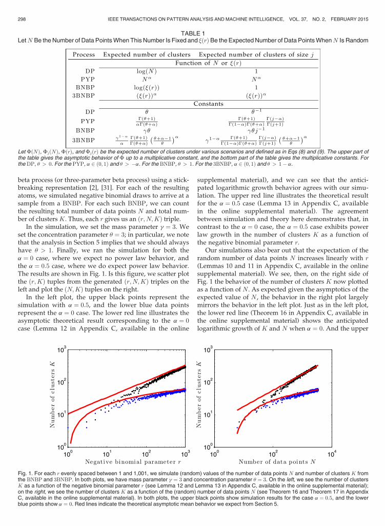
beta process (or three-parameter beta process) using a stick-breaking representation [2], [31]. For each of the resultingatoms, we simulated negative binomial draws to arrive at asample from a BNBP. For each such BNBP, we can countthe resulting total number of data points N and total num-ber of clustersK. Thus, each r gives us an ðr;N;KÞ triple.

In the simulation, we set the mass parameter g ¼ 3. Weset the concentration parameter u ¼ 3; in particular, we notethat the analysis in Section 5 implies that we should alwayshave u > 1. Finally, we ran the simulation for both thea ¼ 0 case, where we expect no power law behavior, andthe a ¼ 0:5 case, where we do expect power law behavior.The results are shown in Fig. 1. Is this figure, we scatter plotthe ðr;KÞ tuples from the generated ðr;N;KÞ triples on theleft and plot the ðN;KÞ tuples on the right.

In the left plot, the upper black points represent thesimulation with a ¼ 0:5, and the lower blue data pointsrepresent the a ¼ 0 case. The lower red line illustrates theasymptotic theoretical result corresponding to the a ¼ 0case (Lemma 12 in Appendix C, available in the online

supplemental material), and we can see that the antici-pated logarithmic growth behavior agrees with our simu-lation. The upper red line illustrates the theoretical resultfor the a ¼ 0:5 case (Lemma 13 in Appendix C, availablein the online supplemental material). The agreementbetween simulation and theory here demonstrates that, incontrast to the a ¼ 0 case, the a ¼ 0:5 case exhibits powerlaw growth in the number of clusters K as a function ofthe negative binomial parameter r.

Our simulations also bear out that the expectation of therandom number of data points N increases linearly with r(Lemmas 10 and 11 in Appendix C, available in the onlinesupplemental material). We see, then, on the right side ofFig. 1 the behavior of the number of clusters K now plottedas a function of N . As expected given the asymptotics of theexpected value of N , the behavior in the right plot largelymirrors the behavior in the left plot. Just as in the left plot,the lower red line (Theorem 16 in Appendix C, available inthe online supplemental material) shows the anticipatedlogarithmic growth of K and N when a ¼ 0. And the upper

TABLE 1LetN Be theNumber of Data PointsWhen This Number Is Fixed and �ðrÞBe the ExpectedNumber of Data PointsWhenN Is Random

Let FðNÞ, FjðNÞ, FðrÞ, and FjðrÞ be the expected number of clusters under various scenarios and defined as in Eqs (8) and (9). The upper part ofthe table gives the asymptotic behavior of F up to a multiplicative constant, and the bottom part of the table gives the multiplicative constants. Forthe DP, u > 0. For the PYP, a 2 ð0; 1Þ and u > �a. For the BNBP, u > 1. For the 3BNBP, a 2 ð0; 1Þ and u > 1� a.

Fig. 1. For each r evenly spaced between 1 and 1,001, we simulate (random) values of the number of data points N and number of clusters K fromthe BNBP and 3BNBP. In both plots, we have mass parameter g ¼ 3 and concentration parameter u ¼ 3. On the left, we see the number of clustersK as a function of the negative binomial parameter r (see Lemma 12 and Lemma 13 in Appendix C, available in the online supplemental material);on the right, we see the number of clusters K as a function of the (random) number of data points N (see Theorem 16 and Theorem 17 in AppendixC, available in the online supplemental material). In both plots, the upper black points show simulation results for the case a ¼ 0:5, and the lowerblue points show a ¼ 0. Red lines indicate the theoretical asymptotic mean behavior we expect from Section 5.


red line (Theorem 17 in Appendix C, available in the onlinesupplemental material) shows the anticipated power lawgrowth ofK andN when a ¼ 0:5.

We can see the parallels with the DP and PYP here. Clus-ters generated from the Dirichlet process (i.e., Pitman-Yorprocess with a ¼ 0) exhibit logarithmic growth of theexpected number of clustersK as the (deterministic) numberof data pointsN grows. And clusters generated from the Pit-man-Yor process with a 2 ð0; 1Þ exhibit power law behaviorin the expectation of K as a function of (fixed) N . So too dowe see that the BNBP, when applied to clustering problems,yields asymptotic growth similar to the DP and that the3BNBP yields asymptotic growth similar to thePYP.

7 POSTERIOR INFERENCE

In this section we present posterior inference algorithms forthe HBNBP. We focus on the setting in which, for each indi-vidual d, there is an associated exchangeable sequence ofobservations ðxd;nÞNd

n¼1. We seek to infer both the admixturecomponent responsible for each observation and the param-eter ck associated with each component. Hereafter, we letzd;n denote the unknown component index associated withxd;n, so that xd;n � F ðczd;n

Þ.Under the HBNBP admixture model introduced in

Section 4, the posterior over component indices andparameters has the form

pðzz�;�;cc� jxx�;�;QÞ / pðzz�;�;cc�;bb0;�;bb�;� jxx�;�;QÞ;where Q , ðF;H; g0; u0; gg �; uu�; rr�Þ is the collection of all fixedhyperparameters. As is the case with HDP admixtures [42]and earlier hierarchical beta process featural models [44],the posterior of the HBNBP admixture cannot be obtainedin analytical form due to complex couplings in the marginalpðxx�;� jQÞ. We therefore develop Gibbs sampling algorithms[11] to draw samples of the relevant latent variables fromtheir joint posterior.

A challenging aspect of inference in the nonparametricsetting is the countable infinitude of component parametersand the countably infinite support of the component indi-ces. We develop two sampling algorithms that cope withthis issue in different ways. In Section 7.1, we use slice sam-pling to control the number of components that need beconsidered on a given round of sampling and therebyderive an exact Gibbs sampler for posterior inference underthe HBNBP admixture model. In Section 7.2, we describe anefficient alternative sampler that makes use of a finiteapproximation to the beta process. Throughout we assumethat the base measure H is continuous. We note that neitherprocedure requires conjugacy between the base distributionH and the data-generating distribution F .

7.1 Exact Gibbs Slice Sampler

Slice sampling [6], [29] has been successfully employed inseveral Bayesian nonparametric contexts, including Dirich-let process mixture modeling [17], [32], [49] and beta pro-cess feature modeling [41]. The key to its success lies in theintroduction of one or more auxiliary variables that serve asadaptive truncation levels for an infinite sum representationof the stochastic process.

This adaptive truncation procedure proceeds as follows.For each observation associated with individual d, we intro-duce an auxiliary variable ud;n with conditional distribution

ud;n � Unifð0; zd;zd;nÞ;

where ðzd;kÞ1k¼1 is a fixed positive sequence with limk!1zd;k ¼ 0. To sample the component indices, we recall that anegative binomial draw id;k � NBðrd; bd;kÞ may be repre-sented as a gamma-Poisson mixture:

�d;k � Gamma rd;1� bd;kbd;k

� �;

id;k � Poisð�d;kÞ:We first sample �d;k from its full conditional. By gamma-Poisson conjugacy, this has the simple form

�d;k � Gamma rd þ id;k; 1=bd;k� �

:

We next note that, given ��d;� and the total number ofobservations associated with individual d, the cluster sizesid;k may be constructed by sampling each zd;n independentlyfrom ��d;�=

Pk �d;k and setting id;k ¼

Pn Iðzd;n ¼ kÞ. Hence,

conditioned on the number of data points Nd, the compo-nent parameters ck, the auxiliary variables �d;k, and theslice-sampling variable ud;n, we sample the index zd;n from adiscrete distribution with

Pðzd;n ¼ kÞ / F ðdxd;n jckÞIðud;n zd;kÞ

zd;k�d;k;

so that only the finite set of component indices fk : zd;k �ud;ng need be considered when sampling zd;n.

Let Kd , maxfk : 9n s.t. zd;k � ud;ng and K , maxdKd.Then, on a given round of sampling, we need only explicitlyrepresent �d;k and bd;k for k Kd and ck and b0;k for k K.The simple Gibbs conditionals for bd;k and ck can be foundin Appendix F.1, available in the online supplemental mate-rial. To sample the shared beta process weights b0;k, weleverage the size-biased construction of the beta processintroduced by Thibaux and Jordan [44]:

B0 ¼X1m¼0

XCm

i¼1

b0;m;idcm;i;� ;

where

Cm �ind Pois u0g0u0 þm

� �; b0;m;i �ind Betað1; u0 þmÞ;

and cm;i;� �iid H;

and we develop a Gibbs slice sampler for generating sam-ples from its posterior. The details are deferred to AppendixF.1, available in the online supplemental material.

7.2 Finite Approximation Gibbs Sampler

An alternative to the size-biased construction ofB0 is a finiteapproximation to the beta process with a fixed number ofcomponents,K:

b0;k �iid Betaðu0g0=K; u0ð1� g0=KÞÞ; ck �iid H;

k 2 f1; . . . ; Kg:(10)


It is known that, when H is continuous, the distribution ofPKk¼1 b0;kdck

converges to BPðu0; g0; HÞ as the number ofcomponents K ! 1 (see the proof of Theorem 3.1 by Hjort[16] with the choice A0ðtÞ ¼ g). Hence, we may leverage thebeta process approximation (10) to develop an approximateposterior sampler for the HBNBP admixture model with anapproximation level K that trades off between computa-tional efficiency and fidelity to the true posterior. We deferthe detailed conditionals of the resulting Gibbs sampler toAppendix F.3, available in the online supplemental mate-rial, and briefly compare the behavior of the finite and exactsamplers on a toy data set in Fig. 2. We note finally that thebeta process approximation in Eq. (10) also gives rise to anew finite admixture model that may be of interest in itsown right; we explore the utility of this HBNBP approxima-tion in Section 9.

8 DOCUMENT TOPIC MODELING

In the next two sections, we show how the HBNBP admix-ture model and its finite approximation can be used as prac-tical building blocks for more complex supervised andunsupervised inferential tasks.

We first consider the unsupervised task of document topicmodeling, in which each individual d is a document contain-ing Nd observations (words) and each word xd;n belongs toa vocabulary of size V . The topic modeling framework is aninstance of admixture modeling in which we assume thateach word of each document is generated from a latentadmixture component or topic, and our goal is to infer thetopic underlying each word.

In our experiments, we let Hord, the C dimension of theordinary component intensity measure, be a Dirichlet distri-bution with parameter h1 for h ¼ 0:1 and 1 a V -dimensionalvector of ones and let F ðckÞ be Multð1;ckÞ. We use the set-ting ðg0; u0; gd; udÞ ¼ ð3; 3; 1; 10Þ for the global and docu-ment-specific mass and concentration parameters and setthe document-specific negative binomial shape parameteraccording to the heuristic rd ¼ Ndðu0 � 1Þ=ðu0g0Þ. We arriveat this heuristic by matching Nd to its expectation under anon-hierarchical BNBPmodel and solving for rd:

E½Nd� ¼ rdE

"X1k¼1

bd;k=ð1� bd;kÞ#¼ g0u0=ðu0 � 1Þ:

When applying the exact Gibbs slice sampler, we let theslice sampling decay sequence follow the same patternacross all documents: zd;k ¼ 1:5�k.

8.1 Worldwide Incidents Tracking System

We report results on the Worldwide Incidents Tracking Sys-tem (WITS) data set.6 This data set consists of reports on79,754 terrorist attacks from the years 2004 through 2010.Each event contains a written summary of the incident, loca-tion information, victim statistics, and various binary fieldssuch as “assassination,” “IED,” and “suicide.” We trans-formed each incident into a text document by concatenatingthe summary and location fields and then adding furtherwords to account for other, categorical fields: e.g., an inci-dent with seven hostages would have the word “hostage”added to the document seven times. We used a vocabularysize of V ¼ 1;048words.

Perpetrator identification. Our experiment assesses theability of the HBNBP admixture model to discriminateamong incidents perpetrated by different organizations.We first grouped documents according to the organizationclaiming responsibility for the reported incident. We con-sidered 5,390 claimed documents in total distributedacross the 10 organizations listed in Table 2. We removedall organization identifiers from all documents and ran-domly set aside 10 percent of the documents in each groupas test data. Next, for each group, we trained an indepen-dent, organization-specific HBNBP model on the remain-ing documents in that group by drawing 10,000 MCMCsamples. We proceeded to classify each test document bymeasuring the likelihood of the document under eachtrained HBNBP model and assigning the label associatedwith the largest likelihood. The resulting confusion matrixacross the 10 candidate organizations is displayed inTable 3a. Results are reported for the exact Gibbs slice

Fig. 2. Number of admixture components used by the finite approximation sampler with K ¼ 100 (left) and the exact Gibbs slice sampler (right) oneach iteration of HBNBP admixture model posterior inference. We use a standard “toy bars” data set with 10 underlying admixture components (cf.[15]). We declare a component to be used by a sample if the sampled beta process weight, b0;k, exceeds a small threshold. Both the exact and thefinite approximation sampler find the correct underlying structure, while the finite sampler attempts to innovate more because of the larger number ofproposal components available to the data in each iteration.

6. https://wits.nctc.gov.


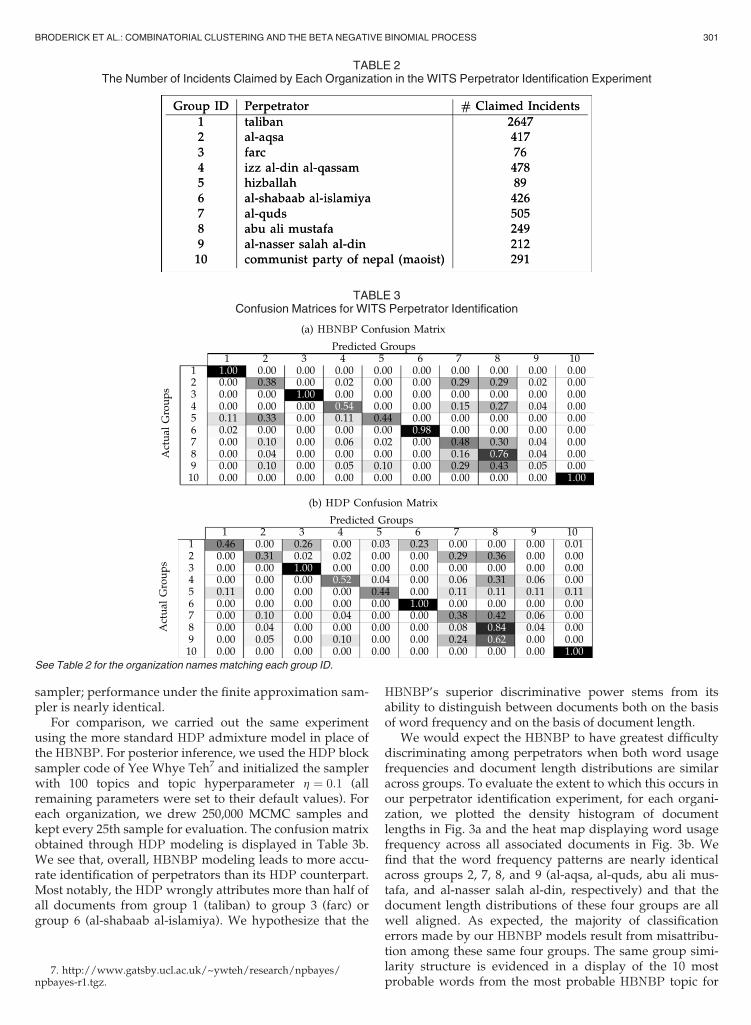
sampler; performance under the finite approximation sam-pler is nearly identical.

For comparison, we carried out the same experimentusing the more standard HDP admixture model in place ofthe HBNBP. For posterior inference, we used the HDP blocksampler code of Yee Whye Teh7 and initialized the samplerwith 100 topics and topic hyperparameter h ¼ 0:1 (allremaining parameters were set to their default values). Foreach organization, we drew 250,000 MCMC samples andkept every 25th sample for evaluation. The confusion matrixobtained through HDP modeling is displayed in Table 3b.We see that, overall, HBNBP modeling leads to more accu-rate identification of perpetrators than its HDP counterpart.Most notably, the HDP wrongly attributes more than half ofall documents from group 1 (taliban) to group 3 (farc) orgroup 6 (al-shabaab al-islamiya). We hypothesize that the

HBNBP’s superior discriminative power stems from itsability to distinguish between documents both on the basisof word frequency and on the basis of document length.

We would expect the HBNBP to have greatest difficultydiscriminating among perpetrators when both word usagefrequencies and document length distributions are similaracross groups. To evaluate the extent to which this occurs inour perpetrator identification experiment, for each organi-zation, we plotted the density histogram of documentlengths in Fig. 3a and the heat map displaying word usagefrequency across all associated documents in Fig. 3b. Wefind that the word frequency patterns are nearly identicalacross groups 2, 7, 8, and 9 (al-aqsa, al-quds, abu ali mus-tafa, and al-nasser salah al-din, respectively) and that thedocument length distributions of these four groups are allwell aligned. As expected, the majority of classificationerrors made by our HBNBP models result from misattribu-tion among these same four groups. The same group simi-larity structure is evidenced in a display of the 10 mostprobable words from the most probable HBNBP topic for

TABLE 2The Number of Incidents Claimed by Each Organization in the WITS Perpetrator Identification Experiment

TABLE 3Confusion Matrices for WITS Perpetrator Identification

See Table 2 for the organization names matching each group ID.

7. http://www.gatsby.ucl.ac.uk/~ywteh/research/npbayes/npbayes-r1.tgz.


each group, Table 4. There, we also find an intuitive sum-mary of the salient regional and methodological vocabularyassociated with each organization.

9 IMAGE SEGMENTATION AND OBJECT

RECOGNITION

Two problems of enduring interest in the computer visioncommunity are image segmentation, dividing an image intoits distinct, semantically meaningful regions, and object rec-ognition, labeling the regions of images according to theirsemantic object classes. Solutions to these problems are atthe core of applications such as content-based imageretrieval, video surveying, and object tracking. Here we will

take an admixture modeling approach to jointly recognizingand localizing objects within images [3], [37], [38], [48]. Eachindividual d is an image comprised of Nd image patches(observations), and each patch xxd;n is assumed to be gener-ated by an unknown object class (a latent component of theadmixture). Given a series of training images with imagepatches labeled, the problem of recognizing and localizingobjects in a new image reduces to inferring the latent classassociated with each new image patch. Since the number ofobject classes is typically known a priori, we will tackle thisinferential task with the finite approximation to the HBNBPadmixture model given in Section 7.2 and compare its per-formance with that of a more standard model of admixture,latent Dirichlet allocation (LDA) [1].

TABLE 4The 10 Most Probable Words from the Most Probable Topic in the Final MCMC Sample of Each

Group in the WITS Perpetrator Identification Experiment.

The topic probability is given in parentheses. See Table 2 for the organization names matching each group ID.

Fig. 3. Document length distributions and word frequencies for each organization in the WITS perpertrator identification experiment.


9.1 Representing an Image Patch

We will represent each image patch as a vector of visualdescriptors drawn from multiple modalities. Verbeek andTriggs [48] suggest three complementary modalities: tex-ture, hue, and location. Here, we introduce a fourth: oppo-nent angle. To describe hue, we use the robust huedescriptor of Van De Weijer and Schmid [47], which grantsinvariance to illuminant variations, lighting geometry, andspecularities. For texture description we use “dense SIFT”features [5], [23], histograms of oriented gradients com-puted not at local keypoints but rather at a single scale overeach patch. To describe coarse location, we cover eachimage with a regular c x c grid of cells (for a total ofV loc ¼ c2 cells) and assign each patch the index of the cover-ing cell. The opponent angle descriptor of Van De Weijerand Schmid [47] captures a second characterization ofimage patch color. These features are invariant to specular-ities, illuminant variations, and diffuse lighting conditions.

To build a discrete visual vocabulary from these rawdescriptors, we vector quantize the dense SIFT, hue, andopponent angle descriptors using k-means, producingV sift, V hue, and V opp clusters respectively. Finally, we formthe observation associated with a patch by concatenatingthe four modality components into a single vector,xxd;n ¼ ðxsift

d;n; xhued;n ; x

locd;n; x

oppd;n Þ. As in [48], we assume that the

descriptors from disparate modalities are conditionallyindependent given the latent object class of thepatch. Hence, we define our data generating distributionand our base distribution over parameters cck ¼ðcsift

k ;chuek ;cloc

k ;coppk Þ via

cmk �ind Dirichletðh1VmÞ for m 2 fsift; hue; loc; oppg

xmd;n j zd;n;cc� �ind Mult

�1;cm

zd;n

�form 2 fsift; hue; loc; oppg

for a hyperparameter h 2 R and 1Vm a V m-dimensional vec-tor of ones.

9.2 Experimental Setup

We use the Microsoft Research Cambridge pixel-wiselabeled image database v1 in our experiments.8 The data setconsists of 240 images, each of size 213 � 320 pixels. Eachimage has an associated pixel-wise ground truth labeling,

with each pixel labeled as belonging to one of 13 semanticclasses or to the void class. Pixels have a ground truth labelof void when they do not belong to any semantic class orwhen they lie on the boundaries between classes in animage. The data set provider notes that there are insuffi-ciently many instances of horse, mountain, sheep, or water tolearn these classes, so, as in Van De Weijer and Schmid [48],we treat these ground truth labels as void as well. Thus, ourgeneral task is to learn and segment the remaining ninesemantic object classes.

From each image, we extract 20 � 20 pixel patchesspaced at 10 pixel intervals across the image. We choose thevisual vocabulary sizes ðV sift; V hue; V loc; V oppÞ ¼ ð1000; 100;100; 100Þ and fix the hyperparameter h ¼ 0:1. As in Verbeekand Triggs [48], we assign each patch a ground truth labelzd;n representing the most frequent pixel label within thepatch. When performing posterior inference, we divide thedata set into training and test images. We allow the infer-ence algorithm to observe the labels of the training imagepatches, and we evaluate the algorithm’s ability to correctlyinfer the label associated with each test image patch.

Since the number of object classes is known a priori, weemploy the HBNBP finite approximation Gibbs sampler ofSection 7.2 to conduct posterior inference. We again use thehyperparameters ðg0; u0; gd; udÞ ¼ ð3; 3; 1; 10Þ for all docu-ments d and set rd according to the heuristic rd ¼Ndðu0 � 1Þ=ðu0g0Þ. We draw 10,000 samples and, for eachtest patch, predict the label with the highest posterior proba-bility across the samples. We compare HBNBP performancewith that of LDA using the standard variational inferencealgorithm of [1] and maximum a posteriori prediction ofpatch labels. For each model, we set K ¼ 10, allowing forthe nine semantic classes plus void, and, following Verbeekand Triggs [48], we ensure that the void class remainsgeneric by fixing cm

10 ¼ ð 1Vm ; � � � ; 1

VmÞ for each modalitym.

9.3 Results

Fig. 4 displays sample test image segmentations obtainedusing the HBNBP admixture model. Each pixel is given thepredicted label of its closest patch center. Test patch classifi-cation accuracies for the HBNBP admixture model andLDA are reported in Tables 5a and 5b respectively. Allresults are averaged over 20 randomly generated 90 percenttraining / 10 percent test divisions of the data set. The two

Fig. 4. MSRC-v1 test image segmentations inferred by the HBNBP admixture model (best viewed in color).

8. http://research.microsoft.com/vision/cambridge/recognition/.


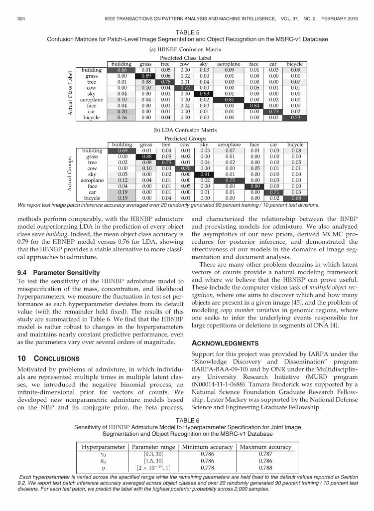
methods perform comparably, with the HBNBP admixturemodel outperforming LDA in the prediction of every objectclass save building. Indeed, the mean object class accuracy is0.79 for the HBNBP model versus 0.76 for LDA, showingthat the HBNBP provides a viable alternative to more classi-cal approaches to admixture.

9.4 Parameter Sensitivity

To test the sensitivity of the HBNBP admixture model tomisspecification of the mass, concentration, and likelihoodhyperparameters, we measure the fluctuation in test set per-formance as each hyperparameter deviates from its defaultvalue (with the remainder held fixed). The results of thisstudy are summarized in Table 6. We find that the HBNBPmodel is rather robust to changes in the hyperparametersand maintains nearly constant predictive performance, evenas the parameters vary over several orders of magnitude.

10 CONCLUSIONS

Motivated by problems of admixture, in which individu-als are represented multiple times in multiple latent clas-ses, we introduced the negative binomial process, aninfinite-dimensional prior for vectors of counts. Wedeveloped new nonparametric admixture models basedon the NBP and its conjugate prior, the beta process,

and characterized the relationship between the BNBPand preexisting models for admixture. We also analyzedthe asymptotics of our new priors, derived MCMC pro-cedures for posterior inference, and demonstrated theeffectiveness of our models in the domains of image seg-mentation and document analysis.

There are many other problem domains in which latentvectors of counts provide a natural modeling frameworkand where we believe that the HBNBP can prove useful.These include the computer vision task of multiple object rec-ognition, where one aims to discover which and how manyobjects are present in a given image [45], and the problem ofmodeling copy number variation in genomic regions, whereone seeks to infer the underlying events responsible forlarge repetitions or deletions in segments of DNA [4].

ACKNOWLEDGMENTS

Support for this project was provided by IARPA under the“Knowledge Discovery and Dissemination” program(IARPA-BAA-09-10) and by ONR under the Multidisciplin-ary University Research Initiative (MURI) program(N00014-11-1-0688). Tamara Broderick was supported by aNational Science Foundation Graduate Research Fellow-ship. Lester Mackey was supported by the National DefenseScience and Engineering Graduate Fellowship.

TABLE 5Confusion Matrices for Patch-Level Image Segmentation and Object Recognition on the MSRC-v1 Database

We report test image patch inference accuracy averaged over 20 randomly generated 90 percent training / 10 percent test divisions.

TABLE 6Sensitivity of HBNBP Admixture Model to Hyperparameter Specification for Joint Image

Segmentation and Object Recognition on the MSRC-v1 Database

Each hyperparameter is varied across the specified range while the remaining parameters are held fixed to the default values reported in Section9.2. We report test patch inference accuracy averaged across object classes and over 20 randomly generated 90 percent training / 10 percent testdivisions. For each test patch, we predict the label with the highest posterior probability across 2,000 samples.


REFERENCES

[1] D. M. Blei, A. Y. Ng, and M. I. Jordan, “Latent Dirichletallocation,” J. Mach. Learn. Res., vol. 3, pp. 993–1022, 2003.

[2] T. Broderick, M. I. Jordan, and J. Pitman, “Beta processes, stick-breaking, and power laws,” Bayesian Anal., vol. 7, pp. 439–476,2012.

[3] L. Cao and F.-F. Li, “Spatially coherent latent topic model for con-current segmentation and classification of objects and scenes,” inProc. IEEE Int. Conf. Comput. Vis., 2007, pp. 1–8.

[4] H. Chen, H. Xing, and N. R. Zhang, “Stochastic segmentationmodels for allele-specific copy number estimation with SNP-arraydata,” PLoS Comput. Biol., vol. 7, p. e1001060, 2011.

[5] N. Dalal and B. Triggs, “Histograms of oriented gradients forhuman detection,” in Proc. Conf. Comput. Vis. Pattern Recog., 2005,pp. 886–893.

[6] P. Damien, J. Wakefield, and S. Walker, “Gibbs sampling forBayesian non-conjugate and hierarchical models by using auxil-iary variables,” J. Roy. Statist. Soc. Series B, vol. 61, pp. 331–344,1999.

[7] E. A. Erosheva and S. E. Fienberg, “Bayesian mixed membershipmodels for soft clustering and classification,” in Classification–TheUbiquitous Challenge, NewYork,NY,USA: Springer, 2005, pp. 11–26.

[8] T. S. Ferguson, “A Bayesian analysis of some nonparametric prob-lems,” Ann. Statist., vol. 1, no. 2, pp. 209–230, 1973.

[9] E. Fox, E. Sudderth, M. Jordan, and A. Willsky, “Sharing featuresamong dynamical systems with beta processes,” Adv. Neural Inf.Process. Syst., vol. 22, pp. 549–557, 2009.

[10] C. Fraley and A. E. Raftery, “Model-based clustering, discriminantanalysis and density estimation,” J. Amer. Statis. Assoc., vol. 97,pp. 611–631, 2002.

[11] S. Geman and D. Geman, “Stochastic relaxation, Gibbs distribu-tions, and the Bayesian restoration of images,” IEEE Pattern Anal.Mach. Intell., vol. PAMI-6, no. 6, pp. 721–741, Nov. 1984.

[12] A. Gnedin, B. Hansen, and J. Pitman, “Notes on the occupancyproblem with infinitely many boxes: General asymptotics andpower laws,” Probability Surveys, vol. 4, pp. 146–171, 2007.

[13] S. Goldwater, T. Griffiths, andM. Johnson, “Interpolating betweentypes and tokens by estimating power-law generators,” in Proc.Adv. Neural Inf. Process. Syst. 18, 2006, vol. 18, pp. 459–466.

[14] T. Griffiths and Z. Ghahramani, “Infinite latent feature modelsand the Indian buffet process,” in Proc. Adv. Neural Inf. Process.Syst. 18, 2006, pp. 475–482.

[15] T. L. Griffiths and M. Steyvers, “Finding scientific topics,” in Proc.Nat. Academy Sci. USA, vol. 101, no. suppl. 1, pp. 5228–5235, Apr.2004.

[16] N. Hjort, “Nonparametric bayes estimators based on beta pro-cesses in models for life history data,” Ann. Statist., vol. 18, no. 3,pp. 1259–1294, 1990.

[17] M. Kalli, J. E. Griffin, and S. G. Walker, “Slice sampling mixturemodels,” Statist. Comput., vol. 21, pp. 93–105, Jan. 2011.

[18] Y. Kim, “Nonparametric Bayesian estimators for counting proc-esses,” Ann. Statist., vol. 27, no. 2, pp. 562–588, 1999.

[19] J. F. C. Kingman, “Completely random measures,” Pacific J. Math.,vol. 21, no. 1, pp. 59–78, 1967.

[20] J. F. C. Kingman, Poisson Processes. New York, NY, USA: OxfordUniv. Press, 1993.

[21] R. M. Korwar and M. Hollander, “Contributions to the theory ofDirichlet processes,” Ann. Probability, vol. 1, pp. 705–711, 1973.

[22] A. Lijoi, R. H. Mena, and I. Pr€unster, “Controlling the reinforce-ment in Bayesian non-parametric mixture models,” J. Roy. Statist.Soc.: Series B (Statist. Methodol.), vol. 69, no. 4, pp. 715–740, 2007.

[23] D. G. Lowe, “Distinctive image features from scale-invariant key-points,” Int. J. Comput. Vis., vol. 60, no. 2, pp. 91–110, 2004.

[24] S. N. MacEachern and P. M€uller, “Estimating mixture of Dirichletprocess models,” J. Comput. Graph. Statist., vol. 7, pp. 223–238,1998.

[25] J. W. McCloskey, “A model for the distribution of individuals byspecies in an environment,” Ph.D. dissertation, Department of Sta-tistics and Probability, Michigan State Univ., East Lansing, MI,USA, 1965.

[26] G. McLachlan and K. Basford, Mixture Models: Inference and Appli-cations to Clustering. New York, NY, USA: Dekker, 1988.

[27] M. Mitzenmacher, “A brief history of generative models forpower law and lognormal distributions,” Internet Math., vol. 1,no. 2, pp. 226–251, 2004.

[28] R. M. Neal, “Markov chain sampling methods for Dirichlet pro-cess mixture models,” J. Comput. Graph. Statist., vol. 9, no. 2,pp. 249–265, 2000.

[29] R. M. Neal, “Slice sampling,” Ann. Statist., vol. 31, no. 3, pp. 705–741, 2003.

[30] M. Newman, “Power laws, Pareto distributions and Zipf’s law,”Contemporary Phys., vol. 46, no. 5, pp. 323–351, 2005.

[31] J. Paisley, A. Zaas, C. W. Woods, G. S. Ginsburg, and L. Carin, “Astick-breaking construction of the beta process,” presented at theInt. Conf. Machine Learning, Haifa, Israel, 2010.

[32] O. Papaspiliopoulos, “A note on posterior sampling from Dirich-let mixture models,” Univ. Warwick, Centre Res. Statist. Meth-odol., Coventry, U.K., Tech. Rep. 8, 2008.

[33] J. Pitman, Combinatorial Stochastic Processes, series LectureNotes in Mathematics. Berlin, Germany: Springer-Verlag, 2006,vol. 1875.

[34] J. Pitman and M. Yor, “The two-parameter Poisson-Dirichlet dis-tribution derived from a stable subordinator,” Ann. Probability,vol. 25, pp. 855–900, 1997.

[35] J. K. Pritchard, M. Stephens, and P. Donnelly, “Inference of popu-lation structure using multilocus genotype data,” Genetics,vol. 155, no. 2, pp. 945–959, 2000.

[36] F. Qi, “Bounds for the ratio of two gamma functions,” J. Inequal-ities Appl., vol. 2010, p. 204, 2010.

[37] B. C. Russell, W. T. Freeman, A. A. Efros, J. Sivic, and A. Zis-serman, “Using multiple segmentations to discover objects andtheir extent in image collections,” in Proc. IEEE Comput. Soc.Conf. Comput. Vis. Pattern Recog., 2006, pp. 1605–1614.

[38] J. Sivic, B. Russell, A. Efros, A. Zisserman, and W. Freeman,“Discovering object categories in image collections,” MIT AI LabMemo, MIT, Cambridge, MA, USA, Tech. Rep. AIM-2005-005,2005..

[39] Y. W. Teh, “A hierarchical Bayesian language model based on pit-man-yor processes,” in Proc. 21st Int. Conf. Comput. Linguistics 44thAnnu. Meet. Assoc. Comput. Linguistics, 2006, pp. 985–992.

[40] Y. W. Teh and D. G€or€ur, “Indian buffet processes with power-lawbehavior,” in Proc. Adv. Neural Inf. Process. Syst. 22, 2009,pp. 1838–1846.

[41] Y. W. Teh, D. G€or€ur, and Z. Ghahramani, “Stick-breaking con-struction for the Indian buffet process,” in Proc. Int. Conf. Artif.Intell. Statist., 2007, vol. 11.

[42] Y. W. Teh, M. I. Jordan, M. J. Beal, and D. M. Blei, “HierarchicalDirichlet processes,” J. Amer. Statist. Assoc., vol. 101, no. 476,pp. 1566–1581, 2006.

[43] R. J. Thibaux, “Nonparametric Bayesian models for machinelearning,” Ph.D. dissertation, EECS Dept., Univ. California, Berke-ley, CA, USA, Oct. 2008.

[44] R. Thibaux and M. Jordan, “Hierarchical beta processes and theIndian buffet process,” in Proc. Int. Conf. Artif. Intell. Statist., 2007,vol. 11.

[45] M. Titsias, “The infinite gamma-Poisson feature model,” in Proc.Adv. Neural Inform. Process. Syst. 20, Cambridge, MA, USA: MITPress, 2008, pp. 1513–1520.

[46] F. G. Tricomi and A. Erd�elyi, “The asymptotic expansion of a ratioof gamma functions,” Pacific. J. Math., vol. 1, no. 1, pp. 133–142,1951.

[47] J. Van De Weijer and C. Schmid, “Coloring local feature extrac-tion,” in Proc. Eur. Conf. Comput. Vis., 2006, pp. 334–348.

[48] J. J. Verbeek and B. Triggs, “Region classification with Markovfield aspect models,” in Proc. IEEE Conf. Comput. Vis. PatternRecog., 2007, pp. 1–8.

[49] S. G. Walker, “Sampling the Dirichlet mixture model with slices,”Commun. Statist.–Simul. Comput., vol. 36, pp. 45–54, 2007.

[50] G. A. Watterson, “The sampling theory of selectively neutralalleles,” Adv. Appl. Probability, vol. 6, pp. 463–488, 1974.

[51] M. West, “Hyperparameter estimation in Dirichlet processmixture models,” Inst. Statist. Decision Sci. DiscussionPaper, Duke Univ., Durham, NC, USA , Tech. Rep. 92-A03,1992.

[52] F. Wood, C. Archambeau, J. Gasthaus, L. James, and Y. W. Teh, “Astochastic memoizer for sequence data,” in Proc. 26th Annu. Int.Conf. Mach. Learn., 2009, pp. 1129–1136.

[53] M. Zhou, L. Hannah, D. Dunson, and L. Carin, “Beta-negativebinomial process and Poisson factor analysis,” in Proc. Int. Conf.Artif. Intell. Statist., 2012, pp. 1462–1471.


Tamara Broderick received the AB degree inmathematics from Princeton University in 2007.On a Marshall Scholarship at the University ofCambridge, she received the master’s ofadvanced study for completion of Part III of theMathematical Tripos in 2008 and the MPhildegree by research in physics in 2009. She iscurrently working toward the PhD degree in sta-tistics from the University of California, Berkeley.Her research interests focus on developing andanalyzing models for unsupervised learning

using Bayesian nonparametrics.

Lester Mackey received the BSE degree in com-puter science from Princeton University, and theMA degree in statistics and PhD degree in com-puter science from the University of California,Berkeley. He was a Simons Math+X postdoctoralfellow at Stanford University and is currently anassistant professor of statistics at Stanford Uni-versity. His recent work focuses on the develop-ment and analysis of algorithms for ranking,matrix factorization, compressed sensing, andadmixture modeling.

John Paisley received the BSE degree in 2004,MS degree in 2007, and the PhD degree in 2010in electrical and computer engineering fromDuke University. He was then a postdoctoralresearcher in the Computer Science Departmentat Princeton University and in the Department ofEECS at UC Berkeley. He is currently an assis-tant professor in the Department of ElectricalEngineering at Columbia University. He works ondeveloping Bayesian models for machine learn-ing applications, particularly for dictionary learn-

ing and topic modeling.

Michael I. Jordan is the Pehong Chen distin-guished professor in the Department of ElectricalEngineering and Computer Science and theDepartment of Statistics at the University of Cali-fornia, Berkeley. His research in recent yearshas focused on Bayesian nonparametric analy-sis, probabilistic graphical models, spectral meth-ods, kernel machines and applications toproblems in statistical genetics, signal process-ing, computational biology, information retrievaland natural language processing. He is a mem-

ber of the National Academy of Sciences, a member of the NationalAcademy of Engineering and a member of the American Academy ofArts and Sciences. He is a Fellow of the American Association for theAdvancement of Science. He has been named a Neyman lecturer and aMedallion lecturer by the Institute of Mathematical Statistics. He is anelected member of the International Institute of Statistics. He is a fellowof the AAAI, ACM, ASA, CSS, IMS, IEEE, and SIAM.

" For more information on this or any other computing topic,please visit our Digital Library at www.computer.org/publications/dlib.


Documents

290 IEEE TRANSACTIONS ON PATTERN ANALYSIS …jwp2128/Papers/BroderickMackeyetal2015.pdf · Combinatorial Clustering and the Beta Negative Binomial Process ... the NBP, and demonstrate