Identifying subtle faults at or below thelimits of seismic resolution and predict-ing fractures associated with folds andflexures is one of the major objectives ofcareful seismic interpretation. With theadvent of common use of 3D seismic inthe late 1980s, first-derivative-based hori-zon dip magnitude and dip azimuth werefound to enhance faults that were other-wise difficult to see. More recently, sec-ond-derivative-based curvature mapshave carried this process a step further.Horizon-based curvature computation isnow available in the commercial work-station environment, putting these toolsin the hands of geoscientists who do nothave access to processing software anddo not have time or inclination to pro-gram.

Background. Seismic interpreters haveused attribute maps for fault interpreta-tion since the introduction of 3D seismicdata. As far back as 1991, Rijks andJaufred showed that dip magnitude anddip azimuth can illuminate subtle faultshaving a displacement significantly lessthan the size of a seismic wavelet. Coher-ence (Bahorich and Farmer, 1995) andSobel-filter-based edge detectors (Luo etal., 1996) measured lateral changes inseismic waveforms and amplitude. Morerecently, curvature attributes have beenfound to be useful in delineating faultsand predicting fracture orientation anddistribution (Roberts, 2001; Hakami etal., 2004). There are different curvaturemeasures that can be used, each havingits own characteristic property. Lisle(1994) discussed the correlation of Gaus-sian curvature to open fractures mea-sured on an outcrop. Hart (2002) showedthat strike curvature is highly correlatedto open fractures in northwestern New Mexico. In contrast,Stevenson (personal communication, 2006) found that thedip component of curvature is correlated to open fracturesin the Austin Chalk Formation of Central Texas.

Ericsson et al. (1988) demonstrated the relationshipbetween production and curvature. While direct predictionof open fractures using curvature requires a significantamount of calibration through the use of production, tracer,image log, or microseismic measurements, curvature imagesalso serve as a powerful aid to conventional structural andstratigraphic interpretation. Curvature is particularly use-ful in mapping faults that are smeared due to inaccuratemigration. Sigismondi and Soldo (2003) have used larger

analysis windows, thereby computing maximum curvatureat different scales to extract subtle features that are muchless obvious from the original time/structure map. Berg-bauer et al. (2003) also compute curvature at different wave-lengths by filtering the input horizon picks in kx-ky space.Al-Dossary and Marfurt (2006) extend this latter concept tovolumetric estimates of curvature by replacing the kx-ky fil-ter with a more tractable x-y convolutional operator.

While volumetric curvature has several significantadvances over horizon-based curvature, not least of whichis circumventing the need to pick regions through which nocontinuous surface exists, we understand that most inter-preters do not have access to such processing software and

Curvature attribute applications to 3D surface seismic dataSATINDER CHOPRA, Arcis Corporation, Calgary, CanadaKURT MARFURT, University of Houston, USA

INTERPRETER’S CORNERCoordinated by Rebecca B. Latimer

404 THE LEADING EDGE APRIL 2007

Figure 1. Impact of filters on a picked horizon. (a) Horizon picked on a 3D seismic volume fromAlberta. (b) Horizon in Figure 1a with one pass of a mean filter. (c) Horizon in 1a with onepass of a median filter (data courtesy of Arcis Corporation).

Figure 2. Impact of filters on the most-negative curvature computation. (center row) Most-negative curvature computed on the seismic horizon shown in Figure 1a. (top row) Most-negative curvature computed on the seismic horizon in Figure 1a with one, two, and threepasses of mean filter. (bottom row) Most-negative curvature computed on the seismic horizonin Figure 1a with one, two, and three passes of median filter (data courtesy of ArcisCorporation).

computer power. In this paper, we therefore attempt to dis-cuss how to use convenient filtering and display techniquesavailable on modern interpretation software to generatehorizon-based curvature estimates of similar quality to hori-zon slices through volumetric estimates.

We illustrate these workflows and discuss their usefulnessin terms of their applications to two 3D seismic volumes, onefrom Alberta and the other from British Columbia, Canada.

Definition and types of curvature. Curvature can be definedas the reciprocal of the radius of a circle that is tangent tothe given curve at a point. Thus curvature will be large fora curve that is “bent more” and will be zero for a straightline. Mathematically, curvature may simply be defined as asecond-order derivative of the curve. If the radii of the cir-cles at the point of contact on the curve are replaced by nor-mal vectors, it is possible to assign a sign to curvature fordifferent shapes, as was proposed by Roberts (2001).Diverging vectors on the curve are associated with anticlines,converging vectors with synclines, and parallel vectors withplanar surfaces (which have zero curvature).

The concept of curvature can be conveniently extendedto three-dimensional surfaces by considering such a surfacebeing intersected by a plane and describing a curve.Curvature can then be calculated at any point on this curve.If a surface is cut by planes that are orthogonal to it, the cur-vature measures are referred to as normal curvatures(Roberts, 2001). Of the family of curves formed this way,there exist just two curves perpendicular to each other—onerepresenting the maximum and the other the minimum cur-vature. Both, with their sign and magnitude, are useful, asfaults can be clearly seen on such displays.

Curvature computation in practice. For most interpretersoperating on a workstation, curvature is usually computedby fitting a quadratic surface z(x, y) of the form

z(x, y) = ax2 + cxy + by2 + dx + ey + f (1)

to an interpreted horizon using least-squares or some otherapproximation method. This yields the coefficients inEquation 1 from which other curvature measures can bederived, such as minimum and maximum curvatures, prin-cipal curvatures, most-positive, most-negative, dip curva-ture, strike curvature, curvedness, and shape index. Becausecurvature is a second derivative of the picked surface, itsapplication to interpreted horizons needs to be done care-fully in that it tends to exacerbate the finer detail and thenoise as well. Horizons picked on noisy surface seismic dataor data contaminated by mis-picks could lead to mislead-ing curvature measures. Consequently, it is advisable to runspatial filtering on horizon surfaces, taking care to removenoise while retaining geologic detail. Most commercial soft-ware provides a basic suite of spatial filters that could beused for this purpose including mean, median, directionalderivative, and sharpening.

The mean filter removes random noise and computes themean or average of the values that fall within the chosen aper-ture. The mean filter applied to an interpreted surfaceenhances long-wavelength and suppresses short-wavelengthcurvature components. Iterative application of a mean filterto a map (i.e., applying the filter successively) will enhancelonger and longer wavelength features. Conversely, if wesubtract this long-wavelength map from the original broad-band wavelength map and then compute curvature on theresidual, we obtain curvature images that enhance short-wavelength features.

The median filter also removes random noise but pre-serves edges, which in the case of a picked horizon willinclude discrete offsets, such as encountered at a fault. Themedian filter can also be applied iteratively, which willreduce random noise in each iteration but will not signifi-cantly increase the high frequency geologic component ofthe surface.

Derivative (sometimes called Sobel) filters increase thehigh-frequency content of the data, and are commonly com-puted using a 3 � 3 mask oriented in a particular directionas shown below:

N–S direction: E–W direction:+1 +2 +1 -1 0 +1

0 0 0 -2 0 +2-1 -2 +1 -1 0 +1

Because curvature is a second-derivative operationapplied to an interpreted surface, adding an additionalderivative only further exacerbates any noise problems.

The sharpening (also call Laplacian) filter computes thesecond derivative of the inline and crossline components ofdip and adds the results. Inspection of the formula pro-vided by Roberts will show that the sharpening filter isclosely related to the mean curvature, discussed below.

To illustrate these filters, we manually picked (line byline) a horizon surface that represents a limestone markerfrom a 3D volume from south central Alberta (Figure 1a).Care was taken to make certain there were no mis-picks. Wethen computed most-negative curvature of this surface with-out filtering (center panel of Figure 2). Note patches show-ing a discrete mesh of faults (white arrow). This horizon wassuccessively passed through a 3 � 3 mean filter (Figure 1b)and the most-negative curvature generated in each pass. Asseen in the upper panel of Figure 2, with each successivepass of the mean filter the background jitter is reduced andfocusing of events increases. The same process was repeatedwith a 3 � 3 median filter (Figure 1c), and the correspond-ing images are shown in the lower panel of Figure 2. As

APRIL 2007 THE LEADING EDGE 405

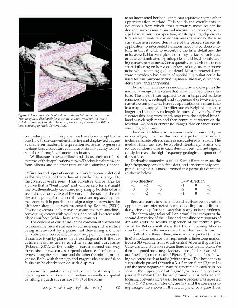
Figure 3. Coherence strat-cube shown intersected by a seismic inline(800 ms of data displayed) for a seismic volume from central–northBritish Columbia, Canada. The size of the survey displayed is 100 km2

(data courtesy of Arcis Corporation).

expected, the median filter smoothes random oscillations butpreserves the major edges in the horizon time/structuremap, resulting in crisper most-negative curvature displays.

Picking the horizon for accurate curvature computation.Blumentritt (2006) found that the quality of volumetric esti-mates of curvature (that precomputed dip and azimuth vol-umes using a finite vertical analysis window of say, +/- 10ms) could be approached better by picking the zero cross-ing. He explains this improvement in that noise added to theflat part of a peak or trough can significantly move theautopick. The same noise added to the much steeper zerocrossing has a much smaller effect. We recommend the fol-lowing workflow: (1) pick the data peak or trough as fits yourwell tie; (2) compute the quadrature of the seismic data; (3)snap the original picks to the zero crossing; (4) compute thecurvature from these snapped picks to the zero crossings.

Because the data at the peak or trough are nearly flat,

moving them slightly will not significantly impact the ampli-tude extractions.

Curvature attributes. In this section, we will discuss theapplication of various curvature attributes to three examples.

Example 1. Figure 3 shows a coherence strat-cube beingintersected by a seismic line from a 3D seismic volume fromcentral-north British Columbia, Canada. Astrat-cube is a sub-volume of seismic data or attributes that are either parallelto a picked horizon (commonly called a flattened subvolume)or interpolated at equal time increments between two non-parallel picked horizons.

A number of faults can be seen on the vertical seismicsection. The top of the coherence strat-cube was chosen tobe the base of Belloy Formation (Figure 4a). We illustratethe basic curvature attributes along the picked Belloy inFigures 4b–d:

Mean curvature is defined as the average of the minimum

406 THE LEADING EDGE APRIL 2007

Figure 4. (a) Horizon time surface. (b) Coherence. (c) Mean curvature. (d) Gaussian curvature. (e) Dip curvature. (f) Strike curvature. (g) Shapeindex. (h) Most-positive curvature. (i) Most-negative curvature. The size of the survey displayed is 100 km2. Approximately 800 ms of data aredisplayed on the vertical seismic section (data courtesy of Arcis Corporation).

and maximum curvature and usually dominated by maxi-mum curvature. Visually, it may not convey any additionalinformation but is useful as other attributes are derivedfrom it. Compared with coherence (Figure 4b), the sign ofmean curvature indicates the high and low shapes (Figure4c), giving a feel for the throw of the faults. Many like thefact that they can estimate fault throw by the change incolor pattern (e.g., Sigismundi and Soldo).

Gaussian curvature is defined as the product of the min-imum and maximum curvatures and gives a measure of dis-tortion of a surface. While this measure has been shown tobe correlated to fractures (Lisle, 1994), it does not show dis-crete faults in this example (Figure 4d) or in the examplepresented by Roberts (2001).

Dip curvature is the curvature extracted along the direc-tion of dip at each analysis point and measures the rate ofchange of dip in the maximum dip direction. As seen inFigure 4e, dip curvature clearly shows the throw and thedirection of the faults. Stevenson finds that dip curvature iscorrelated to open fractures in extensional terrains.

Strike curvature is the curvature extracted along a direc-tion perpendicular to the dip curvature (i.e., along strike ateach analysis point). In Figure 4f, notice how the strike cur-vature indicates patterns connecting high with lows on bothsides of the main fault. In a compressional terrain, Hart etal. (2002) predict that large values of strike curvature willbe correlated to open (versus closed) fractures. In a ten-sional terrain such as the Austin Chalk, others find that dipcurvature correlates with open fractures.

Shape index indicates the local shape of a surface withblue indicating a bowl, cyan a valley, green a saddle, yel-low a ridge, and red a dome (Figure 4g). This attribute is

APRIL 2007 THE LEADING EDGE 407

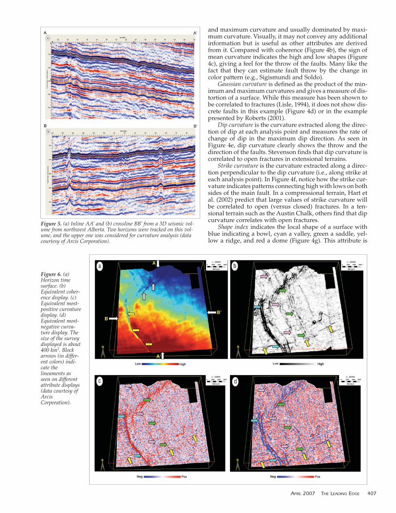
Figure 5. (a) Inline AA’ and (b) crossline BB’ from a 3D seismic vol-ume from northwest Alberta. Two horizons were tracked on this vol-ume, and the upper one was considered for curvature analysis (datacourtesy of Arcis Corporation).

Figure 6. (a)Horizon timesurface. (b)Equivalent coher-ence display. (c)Equivalent most-positive curvaturedisplay. (d)Equivalent most-negative curva-ture display. Thesize of the surveydisplayed is about400 km2. Blockarrows (in differ-ent colors) indi-cate thelineaments asseen on differentattribute displays(data courtesy ofArcisCorporation).

scale independent, meaning that gentle domes and strongdomes will have a similar appearance.

Most-positive curvature defines the curvature that has thegreatest positive value and will show anticlinal and domalfeatures. However, negative values of the most positive cur-vature indicate a bowl feature (Figure 4h).

Most-negative curvature defines the curvature that has thegreatest negative value and will in general highlight syncli-nal and bowl features. However, positive values of the most-negative curvature indicate a dome feature (Figure 4i).

Example 2. Figure 5a shows an inline and a crosslinefrom a 3D seismic volume acquired in northwest Albertafor which we have picked two horizons and generated hori-zon-based curvature attributes. The upper time surface cor-responding to the cyan horizon shown in Figure 5 is shownin Figure 6a and indicates two prominent fault trends, oneat the top trending northeast–southwest (gray arrows) and

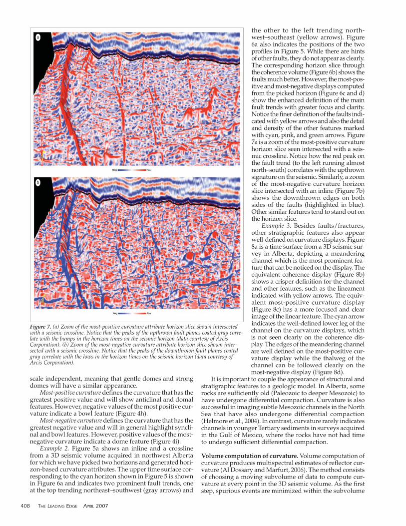
the other to the left trending north-west–southeast (yellow arrows). Figure6a also indicates the positions of the twoprofiles in Figure 5. While there are hintsof other faults, they do not appear as clearly.The corresponding horizon slice throughthe coherence volume (Figure 6b) shows thefaults much better. However, the most-pos-itive and most-negative displays computedfrom the picked horizon (Figure 6c and d)show the enhanced definition of the mainfault trends with greater focus and clarity.Notice the finer definition of the faults indi-cated with yellow arrows and also the detailand density of the other features markedwith cyan, pink, and green arrows. Figure7a is a zoom of the most-positive curvaturehorizon slice seen intersected with a seis-mic crossline. Notice how the red peak onthe fault trend (to the left running almostnorth–south) correlates with the upthrownsignature on the seismic. Similarly, a zoomof the most-negative curvature horizonslice intersected with an inline (Figure 7b)shows the downthrown edges on bothsides of the faults (highlighted in blue).Other similar features tend to stand out onthe horizon slice.

Example 3. Besides faults/fractures,other stratigraphic features also appearwell-defined on curvature displays. Figure8a is a time surface from a 3D seismic sur-vey in Alberta, depicting a meanderingchannel which is the most prominent fea-ture that can be noticed on the display. Theequivalent coherence display (Figure 8b)shows a crisper definition for the channeland other features, such as the lineamentindicated with yellow arrows. The equiv-alent most-positive curvature display(Figure 8c) has a more focused and clearimage of the linear feature. The cyan arrowindicates the well-defined lower leg of thechannel on the curvature displays, whichis not seen clearly on the coherence dis-play. The edges of the meandering channelare well defined on the most-positive cur-vature display while the thalweg of thechannel can be followed clearly on themost-negative display (Figure 8d).

It is important to couple the appearance of structural andstratigraphic features to a geologic model. In Alberta, somerocks are sufficiently old (Paleozoic to deeper Mesozoic) tohave undergone differential compaction. Curvature is alsosuccessful in imaging subtle Mesozoic channels in the NorthSea that have also undergone differential compaction(Helmore et al., 2004). In contrast, curvature rarely indicateschannels in younger Tertiary sediments in surveys acquiredin the Gulf of Mexico, where the rocks have not had timeto undergo sufficient differential compaction.

Volume computation of curvature. Volume computation ofcurvature produces multispectral estimates of reflector cur-vature (Al Dossary and Marfurt, 2006). The method consistsof choosing a moving subvolume of data to compute cur-vature at every point in the 3D seismic volume. As the firststep, spurious events are minimized within the subvolume

408 THE LEADING EDGE APRIL 2007

Figure 7. (a) Zoom of the most-positive curvature attribute horizon slice shown intersectedwith a seismic crossline. Notice that the peaks of the upthrown fault planes coated gray corre-late with the bumps in the horizon times on the seismic horizon (data courtesy of ArcisCorporation). (b) Zoom of the most-negative curvature attribute horizon slice shown inter-sected with a seismic crossline. Notice that the peaks of the downthrown fault planes coatedgray correlate with the lows in the horizon times on the seismic horizon (data courtesy ofArcis Corporation).

and dip components are computed. Next, fractional deriv-atives are computed within the subvolume to investigatemultiple wavelengths of curvature; short wavelengths cor-respond to intense, but highly localized fracture systems,and longer wavelengths to a wider and even distributionof fractures. Short-wavelength estimates of curvature couldincorporate dip information of 9–25 traces; the long-wave-length estimates of curvature could use dip information of400 or more traces. Fractional derivatives are thus appliedalong each time slice with dip components previously esti-mated at each seismic bin to yield estimates of curvature.

Volume curvature estimates eliminate interpretationproblems and allow us to extract curvature measures alonghorizons, thereby helping understand the subsurface fea-tures better.

Example 1. Figure 9a shows the strat-slice from the most-positive curvature volume 30 ms below the horizon in Figure4. The horizon at this level is not easy to track and so the

attribute volume helps in studying the fault patterns at thislevel. Similarly, the equivalent strat-slice extracted from themost-negative curvature volume is shown in Figure 9b.Notice, the fault pattern is somewhat different at this level,and these patterns can be studied carefully in the zone ofinterest.

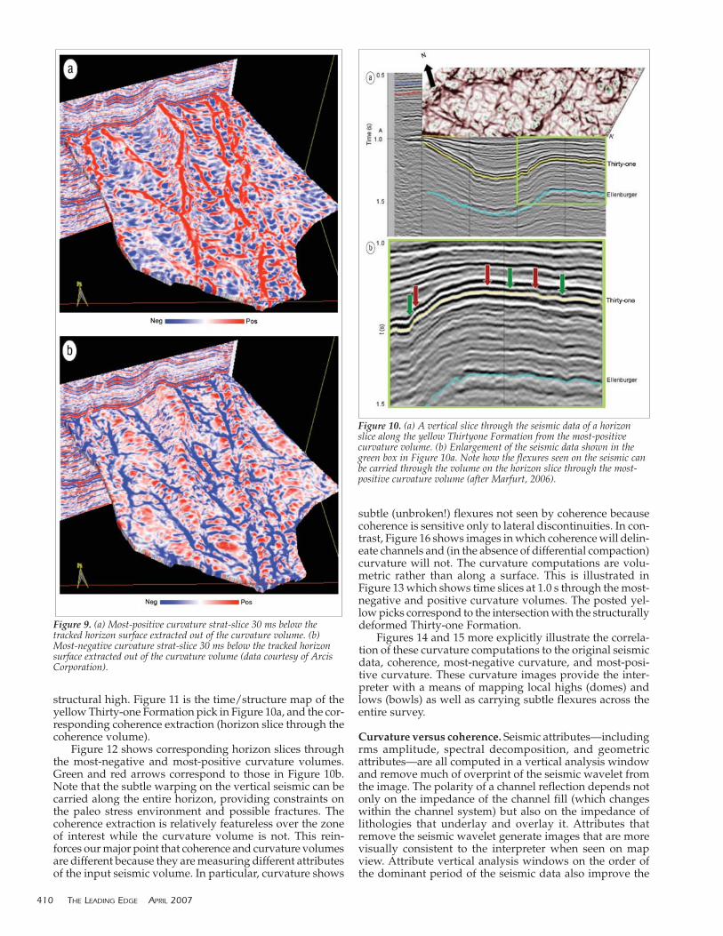
Example 2. This example is from a survey over the CentralBasin Platform of West Texas. The major production in thisarea is from the Devonian-age Thirty-one Formation, a chertdeposit carried from the shelf in the north by turbidity flowsinto this deeper part of basin. The reservoir is highly com-partmentalized and is enhanced by fractures. Figure 10a isan image of the most-positive curvature extracted along theyellow Thirty-one Formation horizon posted on the verti-cal slice through the seismic data. Figure 10b is an enlargedview of the seismic data corresponding to a producing partof the reservoir (green box in Figure 10a). Green arrows indi-cate synclinal and red arrows anticlinal features within this

APRIL 2007 THE LEADING EDGE 409

Figure 8. (a) Time surface. (b) Coherence. (c) Most-positive curvature. (d) Most-negative curvature. Curvature attributes indicate a better focus-ing of the base and edges of the channels and other features as compared with coherence. Yellow arrows indicate a linear feature on the coherence,but the same feature appears crisper on the most-positive curvature display. Cyan arrow indicates the well-defined lower leg of the channel on thecurvature displays, which is not seen clearly on the coherence display. The edges of the meandering channel are defined well throughout the most-positive curvature display and the base of channel can be followed clearly on the most-negative display (data courtesy of Arcis Corporation).

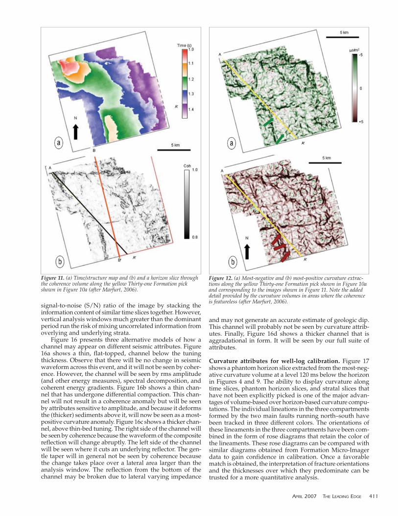
structural high. Figure 11 is the time/structure map of theyellow Thirty-one Formation pick in Figure 10a, and the cor-responding coherence extraction (horizon slice through thecoherence volume).

Figure 12 shows corresponding horizon slices throughthe most-negative and most-positive curvature volumes.Green and red arrows correspond to those in Figure 10b.Note that the subtle warping on the vertical seismic can becarried along the entire horizon, providing constraints onthe paleo stress environment and possible fractures. Thecoherence extraction is relatively featureless over the zoneof interest while the curvature volume is not. This rein-forces our major point that coherence and curvature volumesare different because they are measuring different attributesof the input seismic volume. In particular, curvature shows

subtle (unbroken!) flexures not seen by coherence becausecoherence is sensitive only to lateral discontinuities. In con-trast, Figure 16 shows images in which coherence will delin-eate channels and (in the absence of differential compaction)curvature will not. The curvature computations are volu-metric rather than along a surface. This is illustrated inFigure 13 which shows time slices at 1.0 s through the most-negative and positive curvature volumes. The posted yel-low picks correspond to the intersection with the structurallydeformed Thirty-one Formation.

Figures 14 and 15 more explicitly illustrate the correla-tion of these curvature computations to the original seismicdata, coherence, most-negative curvature, and most-posi-tive curvature. These curvature images provide the inter-preter with a means of mapping local highs (domes) andlows (bowls) as well as carrying subtle flexures across theentire survey.

Curvature versus coherence. Seismic attributes—includingrms amplitude, spectral decomposition, and geometricattributes—are all computed in a vertical analysis windowand remove much of overprint of the seismic wavelet fromthe image. The polarity of a channel reflection depends notonly on the impedance of the channel fill (which changeswithin the channel system) but also on the impedance oflithologies that underlay and overlay it. Attributes thatremove the seismic wavelet generate images that are morevisually consistent to the interpreter when seen on mapview. Attribute vertical analysis windows on the order ofthe dominant period of the seismic data also improve the

410 THE LEADING EDGE APRIL 2007

Figure 9. (a) Most-positive curvature strat-slice 30 ms below thetracked horizon surface extracted out of the curvature volume. (b)Most-negative curvature strat-slice 30 ms below the tracked horizonsurface extracted out of the curvature volume (data courtesy of ArcisCorporation).

Figure 10. (a) A vertical slice through the seismic data of a horizonslice along the yellow Thirtyone Formation from the most-positivecurvature volume. (b) Enlargement of the seismic data shown in thegreen box in Figure 10a. Note how the flexures seen on the seismic canbe carried through the volume on the horizon slice through the most-positive curvature volume (after Marfurt, 2006).

signal-to-noise (S/N) ratio of the image by stacking theinformation content of similar time slices together. However,vertical analysis windows much greater than the dominantperiod run the risk of mixing uncorrelated information fromoverlying and underlying strata.

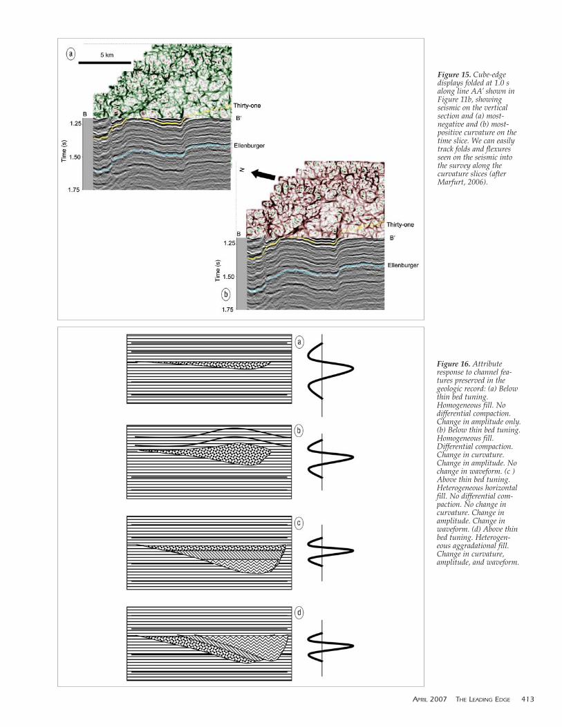
Figure 16 presents three alternative models of how achannel may appear on different seismic attributes. Figure16a shows a thin, flat-topped, channel below the tuningthickness. Observe that there will be no change in seismicwaveform across this event, and it will not be seen by coher-ence. However, the channel will be seen by rms amplitude(and other energy measures), spectral decomposition, andcoherent energy gradients. Figure 16b shows a thin chan-nel that has undergone differential compaction. This chan-nel will not result in a coherence anomaly but will be seenby attributes sensitive to amplitude, and because it deformsthe (thicker) sediments above it, will now be seen as a most-positive curvature anomaly. Figure 16c shows a thicker chan-nel, above thin-bed tuning. The right side of the channel willbe seen by coherence because the waveform of the compositereflection will change abruptly. The left side of the channelwill be seen where it cuts an underlying reflector. The gen-tle taper will in general not be seen by coherence becausethe change takes place over a lateral area larger than theanalysis window. The reflection from the bottom of thechannel may be broken due to lateral varying impedance

and may not generate an accurate estimate of geologic dip.This channel will probably not be seen by curvature attrib-utes. Finally, Figure 16d shows a thicker channel that isaggradational in form. It will be seen by our full suite ofattributes.

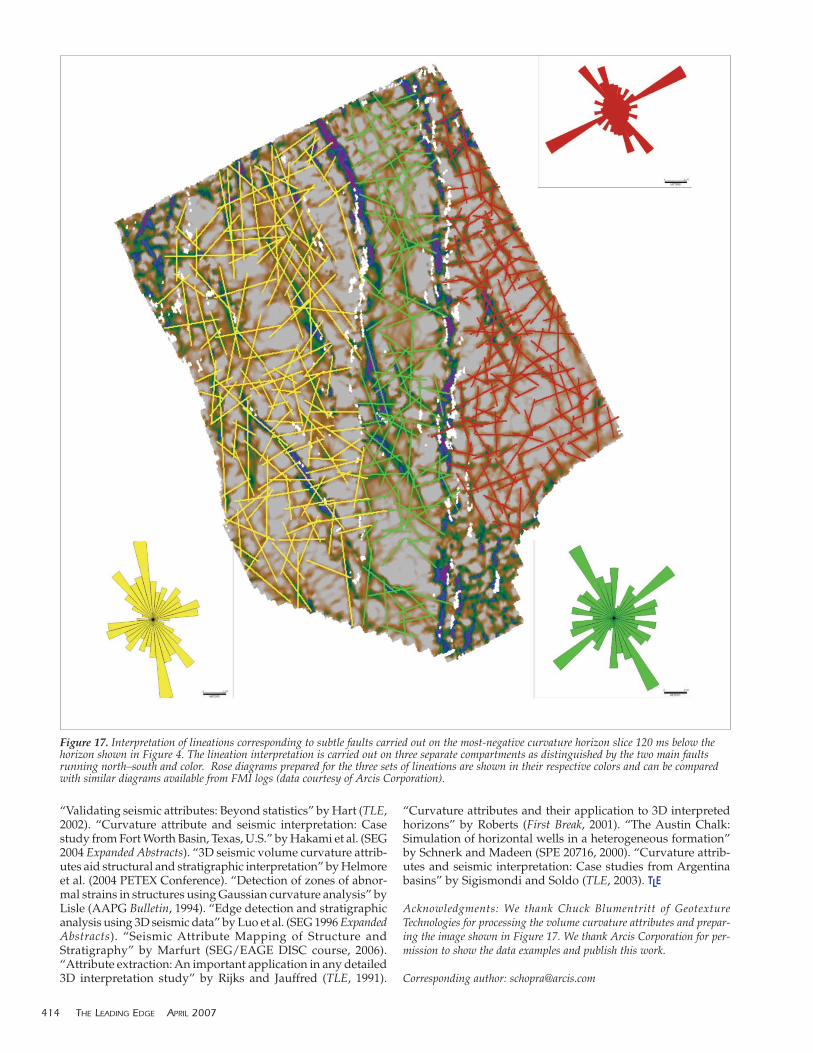
Curvature attributes for well-log calibration. Figure 17shows a phantom horizon slice extracted from the most-neg-ative curvature volume at a level 120 ms below the horizonin Figures 4 and 9. The ability to display curvature alongtime slices, phantom horizon slices, and stratal slices thathave not been explicitly picked is one of the major advan-tages of volume-based over horizon-based curvature compu-tations. The individual lineations in the three compartmentsformed by the two main faults running north–south havebeen tracked in three different colors. The orientations ofthese lineaments in the three compartments have been com-bined in the form of rose diagrams that retain the color ofthe lineaments. These rose diagrams can be compared withsimilar diagrams obtained from Formation Micro-Imagerdata to gain confidence in calibration. Once a favorablematch is obtained, the interpretation of fracture orientationsand the thicknesses over which they predominate can betrusted for a more quantitative analysis.

APRIL 2007 THE LEADING EDGE 411

Figure 11. (a) Time/structure map and (b) and a horizon slice throughthe coherence volume along the yellow Thirty-one Formation pickshown in Figure 10a (after Marfurt, 2006).

Figure 12. (a) Most-negative and (b) most-positive curvature extrac-tions along the yellow Thirty-one Formation pick shown in Figure 10aand corresponding to the images shown in Figure 11. Note the addeddetail provided by the curvature volumes in areas where the coherenceis featureless (after Marfurt, 2006).

Conclusions. Curvature attributes provide images of struc-ture and stratigraphy that complement those seen by thewell-accepted coherence algorithms. Being second-orderderivative measures of surfaces, they can be quite sensitiveto noise. Picks made on zero-crossings (on the quadratureof the data if appropriate) are in general less noisy than thosemade on peaks and troughs. Additional noise can be sup-pressed by iteratively running spatial filtering on horizonsurfaces. Mean filters seem to do a satisfactory job and helpenhance long-wavelength curvature features that may be dif-ficult to see on the picked horizon itself. Median filterssharpen discrete horizon discontinuities such as faults.

For the data sets under study, strike curvature, shapeindex, most-positive, and most-negative curvature offeredbetter interpretation of subtle fault detail than other attrib-utes. Volume curvature attributes provide valuable infor-mation on fracture orientation and density in zones whereseismic horizons are not trackable. The orientations of thefault/fracture lineations interpreted on curvature displayscan be combined in the form of rose diagrams, which in turncan be compared with similar diagrams obtained from FMIdata to gain confidence in calibration.

Suggested reading. “3D volumetric multispectral estimates ofreflector curvature and rotation” by Al-Dossary and Marfurt(GEOPHYSICS, 2006). “3D seismic coherency for faults and strati-graphic features” by Bahorich and Farmer (TLE, 1995).“Improving curvature analyses of deformed horizons usingscale-dependent filtering techniques” by Bergbauer et al. (AAPGBulletin, 2003). “Volume-based curvature analysis illuminatesfracture orientations” by Blumentritt (AAPG 2005 AnnualConvention). Seismic Attributes for Prospect Identification andReservoir Characterization by Chopra and Marfurt (SEG, in press).“Facies and curvature controlled 3D fracture models in aCretaceous carbonate reservoir, Arabian Gulf” by Ericsson etal. (in Faulting, Fault Sealing and Fluid Flow in HydrocarbonReservoirs, Geological Society Special Publication 147, 1988).

412 THE LEADING EDGE APRIL 2007

Figure 13. Time slice at 1.0 s through (a) most-negative and (b) most-positive curvature volumes. The yellow picks correspond to intersec-tions of the time slice with the Thirty-one Formation shown in Figure10a. Folds and flexures can be interpreted on these time slices prior topicking any horizons (after Marfurt, 2006).

Figure 14. Cube-edgedisplays folded at 1.0 salong line AA’ shown inFigure 11b, showing seis-mic on the vertical sectionand (a) seismic and (b)coherence on the time slice.The zone of intersection isrelatively featureless on thecoherence slice (afterMarfurt, 2006).

APRIL 2007 THE LEADING EDGE 413

Figure 15. Cube-edgedisplays folded at 1.0 salong line AA’ shown inFigure 11b, showingseismic on the verticalsection and (a) most-negative and (b) most-positive curvature on thetime slice. We can easilytrack folds and flexuresseen on the seismic intothe survey along thecurvature slices (afterMarfurt, 2006).

Figure 16. Attributeresponse to channel fea-tures preserved in thegeologic record: (a) Belowthin bed tuning.Homogeneous fill. Nodifferential compaction.Change in amplitude only.(b) Below thin bed tuning.Homogeneous fill.Differential compaction.Change in curvature.Change in amplitude. Nochange in waveform. (c )Above thin bed tuning.Heterogeneous horizontalfill. No differential com-paction. No change incurvature. Change inamplitude. Change inwaveform. (d) Above thinbed tuning. Heterogen-eous aggradational fill.Change in curvature,amplitude, and waveform.

“Validating seismic attributes: Beyond statistics” by Hart (TLE,2002). “Curvature attribute and seismic interpretation: Casestudy from Fort Worth Basin, Texas, U.S.” by Hakami et al. (SEG2004 Expanded Abstracts). “3D seismic volume curvature attrib-utes aid structural and stratigraphic interpretation” by Helmoreet al. (2004 PETEX Conference). “Detection of zones of abnor-mal strains in structures using Gaussian curvature analysis” byLisle (AAPG Bulletin, 1994). “Edge detection and stratigraphicanalysis using 3D seismic data” by Luo et al. (SEG 1996 ExpandedAbstracts). “Seismic Attribute Mapping of Structure andStratigraphy” by Marfurt (SEG/EAGE DISC course, 2006).“Attribute extraction: An important application in any detailed3D interpretation study” by Rijks and Jauffred (TLE, 1991).

“Curvature attributes and their application to 3D interpretedhorizons” by Roberts (First Break, 2001). “The Austin Chalk:Simulation of horizontal wells in a heterogeneous formation”by Schnerk and Madeen (SPE 20716, 2000). “Curvature attrib-utes and seismic interpretation: Case studies from Argentinabasins” by Sigismondi and Soldo (TLE, 2003). TLE

Acknowledgments: We thank Chuck Blumentritt of GeotextureTechnologies for processing the volume curvature attributes and prepar-ing the image shown in Figure 17. We thank Arcis Corporation for per-mission to show the data examples and publish this work.

Corresponding author: schopra@arcis.com

414 THE LEADING EDGE APRIL 2007

Figure 17. Interpretation of lineations corresponding to subtle faults carried out on the most-negative curvature horizon slice 120 ms below thehorizon shown in Figure 4. The lineation interpretation is carried out on three separate compartments as distinguished by the two main faultsrunning north–south and color. Rose diagrams prepared for the three sets of lineations are shown in their respective colors and can be comparedwith similar diagrams available from FMI logs (data courtesy of Arcis Corporation).