25/6/2006

Solving Multivariate Nonlinear Polynomial Systems

Massarwi Fady

Computer Aided Geometric Design (236716)

Spring 2006

25/6/2006

References "Computation of the solutions of nonlinear polynomial

systems", by E. C. Sherbrooke and N. M. patrikalakis. Computer Aided Geometric Design, Vol 10, No 5, pp 379-405, 1993

"Geometric Constraint Solver using Multivariate Rational Spline Functions", by G. Elber and M. S. Kim. The Sixth ACM/IEEE Symposium on Solid Modeling and Applications, Ann Arbor, Michigan, pp 1-10, June 2001.

"Subdivision methods for solving polynomial equations", by B. Mourrain and J. P. Pavone, Technical Report 5658, Inria, Sophia-Antipolis, 2005.

25/6/2006

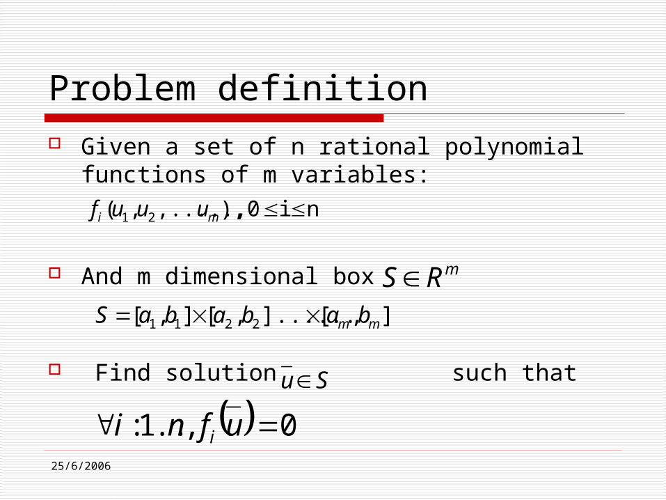
Problem definition Given a set of n rational polynomial

functions of m variables:

And m dimensional box

Find solution such that

ni0 ),,.....,,( 21 mi uuuf

Su

0,..1: ufni i

],[]......,[],[ 2211 mm bababaS

mRS

25/6/2006

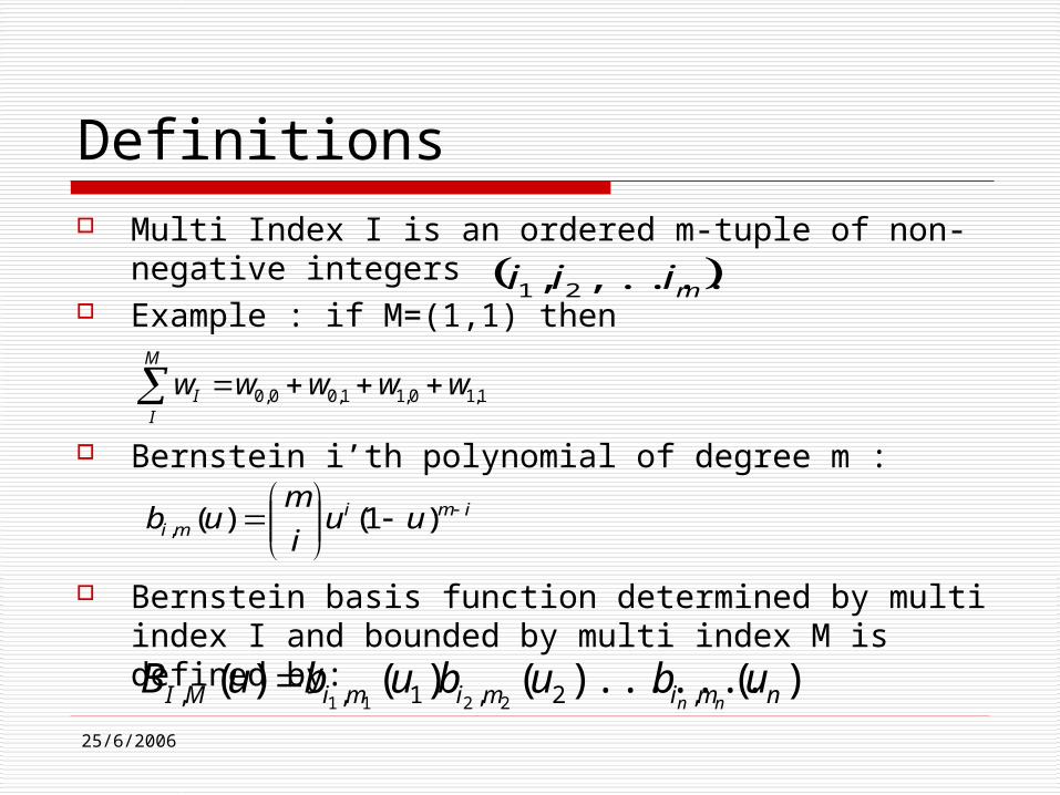
Definitions Multi Index I is an ordered m-tuple of non-negative

integers Example : if M=(1,1) then

Bernstein i’th polynomial of degree m :

Bernstein basis function determined by multi index I and bounded by multi index M is defined by:

miii ,....,, 21

1,10,11,00,0 wwwwwM

II

imimi uu

i

mub

)1()(,

)().......()()( ,2,1,, 2211 nmimimiMI ubububuBnn

25/6/2006

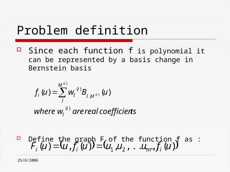
Problem definition Since each function f is polynomial it can be

represented by a basis change in Bernstein basis

Define the graph F of the function f as :

tscoefficien realarewwhere

uBwuf

iI

M

IMI

iIi

i

i

)()(

)(

,

)()(

)(

)(,,....,,)(,)( 21 ufuuuufuuF imii

25/6/2006

Problem definition Since

We can write

And write the graph F of each function as :

The set of V are the control points of F, this representation is much powerful and allows to use different properties of Bernstein basis ( like convex hull property )

u is a solution to the polynomial system if the point (u,0) contained in all the graphs Fi

m

imi xb

m

ix

0, )(

)(

)( )(,)(

k

k

M

IMIk

j

jj uB

m

iu

)()()(

2

2)(

1

1)(

,

)(

,,.....,,

)()( )(

)(

kIk

n

nkk

kI

MI

M

I

kIk

wm

i

m

i

m

ivwhere

uBvuF k

k

25/6/2006

Subdivision-based techniques Numerical methods to find areas (box) where a single

root ( solution ) could be found In each step, If the current box dimensions are larger

than some tolerance split it into two boxes and search in each of them recursively.

Advantages: Speed Stability Simple

Disadvantages: Designed for zero dimensional solution set -- No

guarantee that all the roots are found Doesn’t supply information on the root multiplicity

25/6/2006

Subdivision-based techniques We will review The following:

Subdivision while restricting the search domain PP ( projection polyhedron ) , LP (linear

programming ) - ( Sherbrooke & Patrikalakis) Subdivision with numerical improvements ( Elber

& Kim ) Usage examples

Further improvements ( Mourrain & Pavoni)

25/6/2006

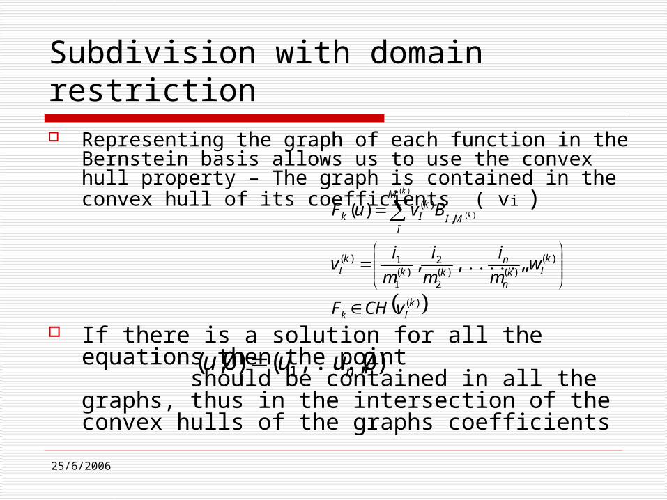
Subdivision with domain restriction Representing the graph of each function in the

Bernstein basis allows us to use the convex hull property – The graph is contained in the convex hull of its coefficients ( vi )

If there is a solution for all the equations then the point should be contained in all the graphs, thus in the intersection of the convex hulls of the graphs coefficients

)(

)()()(

2

2)(

1

1)(

,

)(

,,.....,,

)( )(

)(

kIk

kIk

n

nkk

kI

MI

M

I

kIk

vCHF

wm

i

m

i

m

iv

BvuF k

k

)0,,...,()0,( 1 nuuu

25/6/2006

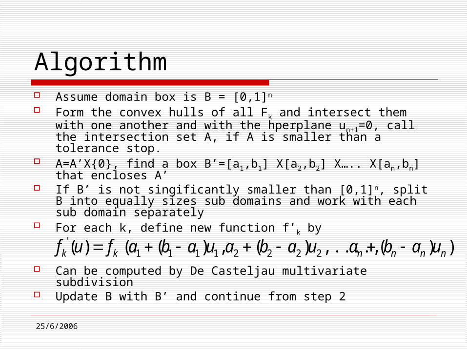
Algorithm Assume domain box is B = [0,1]n Form the convex hulls of all Fk and intersect them with

one another and with the hperplane un+1=0, call the intersection set A, if A is smaller than a tolerance stop.

A=A’X{0}, find a box B’=[a1,b1] X[a2,b2] X….. X[an,bn] that encloses A’

If B’ is not singificantly smaller than [0,1]n, split B into equally sizes sub domains and work with each sub domain separately

For each k, define new function f’k by

Can be computed by De Casteljau multivariate subdivision

Update B with B’ and continue from step 2

))(,....,)(,)(()( 22221111'

nnnnkk uabauabauabafuf

25/6/2006

Algorithm ( cont’d) Step 2 contains two heavy operations

Computing the convex hull in dimension n

Intersecting all the convex hulls

Actually what we need is the bounding box of the intersection of the convex hulls, this can be achieved in different simple way

25/6/2006

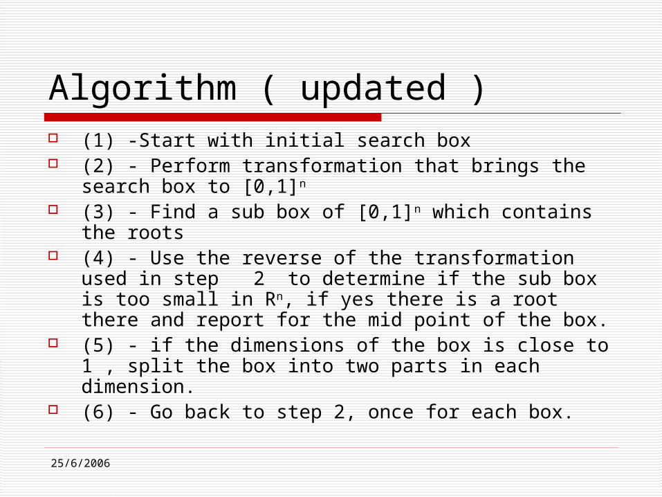
Algorithm ( updated ) (1) -Start with initial search box (2) - Perform transformation that brings the search

box to [0,1]n

(3) - Find a sub box of [0,1]n which contains the roots (4) - Use the reverse of the transformation used in

step 2 to determine if the sub box is too small in Rn, if yes there is a root there and report for the mid point of the box.

(5) - if the dimensions of the box is close to 1 , split the box into two parts in each dimension.

(6) - Go back to step 2, once for each box.

25/6/2006

Finding the Bounding Box of the intersection of the CHs Projected Polyhedron ( PP )

Find the width of the bounding box in each dimension by projecting it in that dimension

For dimension j: For each graph Fk project each of it’s control points u

to (uj,un+1) ( call it x-y plane ) Form the convex hull in 2d of the projected points Return as [aj,bj] the intersection of the convex hull

with the X axis in the projection plane ( between 0 and 1 for all the graphs ).

Finally the bounding box will be B = [a1,b1]X [a2,b2]X…… X[an,bn]

25/6/2006

Finding the Bounding Box of the intersection of the CHs

Linear Programming ( LP ) minimization function - If we look at the

i’th coordinate of the points lying in the feasible area , what is the smallest ( ai ), and what is the biggest ( bi )

Constrains – for each point x in the feasible area , it must satisfy xn+1 =0 For each k between 1 and n , x is contained

in the convex hull of Vk (the control points of Fk)

25/6/2006

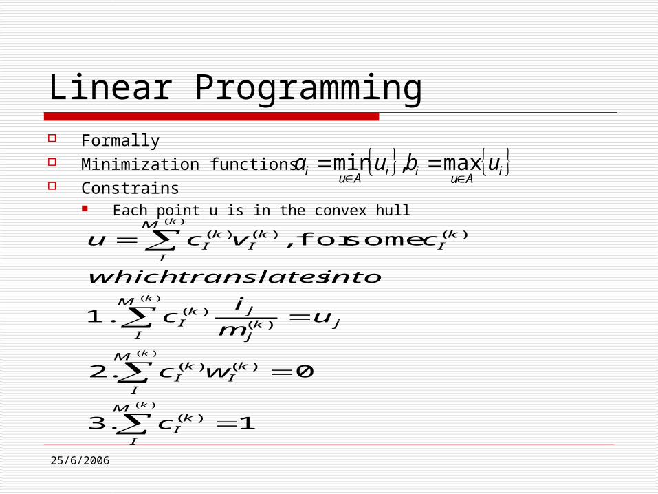
Linear Programming Formally Minimization functions: Constrains

Each point u is in the convex hull

iAu

iiAu

i ubua

max,min

)(

)(

)(

)(

1.3

0.2

. 1

somefor ,

)(

)()(

)()(

)()()(

k

k

k

k

M

I

kI

M

I

kI

kI

M

Ijk

j

jkI

kI

M

I

kI

kI

c

wc

um

ic

into translates which

cvcu

25/6/2006

Linear Programming The unknowns are the coefficients The number of the unknowns is

)(kIc

n

k

kn

kk mmm1

)()(2

)(1 )1()1)(1(

25/6/2006

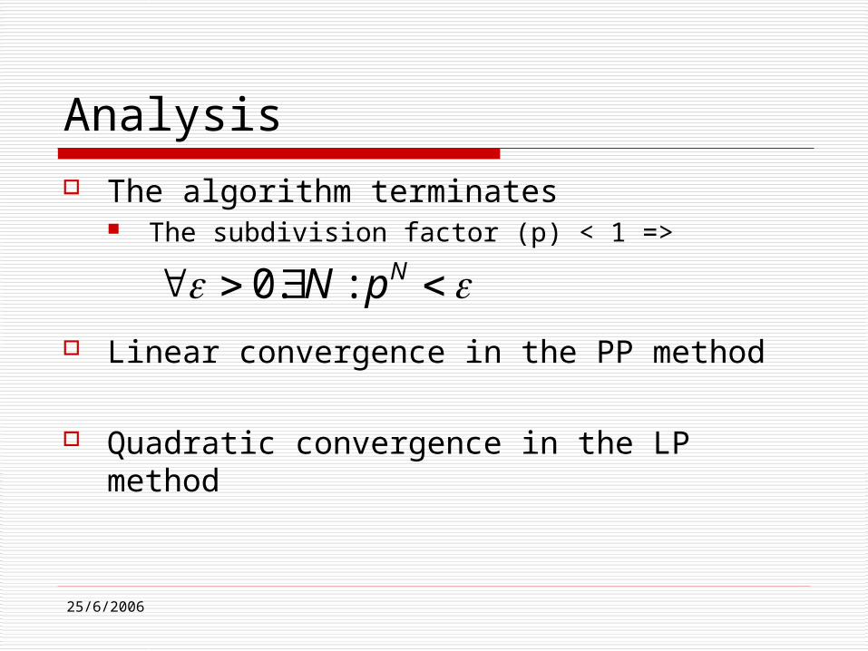
Analysis The algorithm terminates

The subdivision factor (p) < 1 =>

Linear convergence in the PP method

Quadratic convergence in the LP method

NpN :.0

25/6/2006

Linear convergence in the PP method

Given a box B=[a1,b1]x[a2,b2]x…x[an,bn] which contains one and only one simple root x0 of a system of polynomials f0,k:[0,1]nR where k ranges from 1 to n. let fk represent the subdivision of f0,k over B. Let the new box after executing one step of the PP method, denoted by B’=[a’1,b’1]x[a’2,b’2]x…x[a’n,b’n].Let j be an integer between 1 and n, and let

( the lengths of the j’th side ) then jjjj abab ''' and

)(' O

25/6/2006

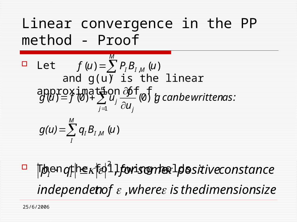
Linear convergence in the PP method - Proof

Let and g(u) is the linear approximation of f,

Then the following holds :

M

IMII uBPuf )()( ,

M

IMII

j

n

jj

uBqg(u)

: as writtenbe can g u

fufug

)(

),0()0()(

,

1

size dimension the is where of tindependen

constance positive somefor qp II

,

,2

25/6/2006

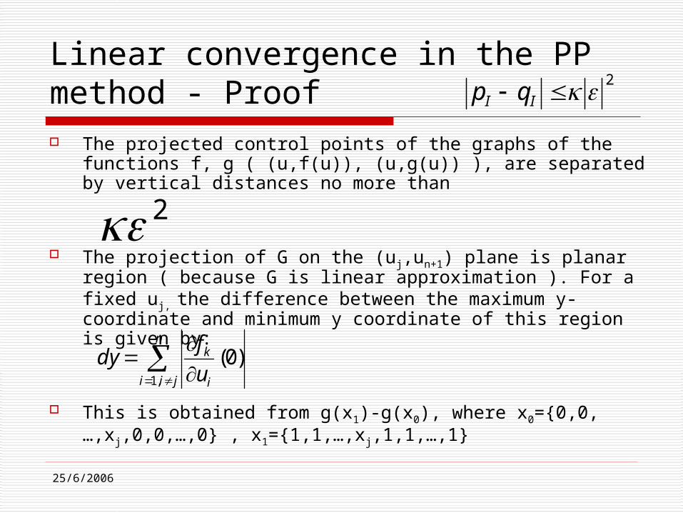
Linear convergence in the PP method - Proof The projected control points of the graphs of the functions

f, g ( (u,f(u)), (u,g(u)) ), are separated by vertical distances no more than

The projection of G on the (uj,un+1) plane is planar region ( because G is linear approximation ). For a fixed uj, the difference between the maximum y-coordinate and minimum y coordinate of this region is given by:

This is obtained from g(x1)-g(x0), where x0={0,0,…,xj,0,0,…,0} , x1={1,1,…,xj,1,1,…,1}

2

2 II qp

n

jii i

k

u

fdy

,1

)0(

25/6/2006

Linear convergence in the PP method - Proof

Then we can say that the whole projected control points of F are enclosed by two parallel lines that has a distance of from each other and slope of

Then if we look at the intersection of these two lines with the x axis ( between 0 and 1), the distance between the intersections ( which is translated to the box dimension later ) is :

)0(

2 2

juf

dydx

22dy)0(

ju

f

25/6/2006

Linear convergence in the PP method - Proof Since

But we do scaling to transform the box to Rn, by scaling by , and this is the new box we work with so the new box dimension is

)0(

2 2

juf

dydx

)1(

)(

),(

Odx

Ou

f

Ody

j

)(O

)()0()0( ,0

,1i

i

k

i

kn

jii i

k au

f

u

f and

u

fdy

25/6/2006

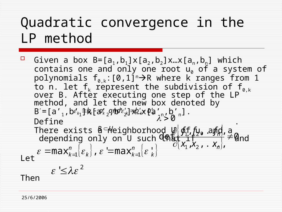
Quadratic convergence in the LP method Given a box B=[a1,b1]x[a2,b2]x…x[an,bn] which

contains one and only one root u0 of a system of polynomials f0,k:[0,1]nR where k ranges from 1 to n. let fk represent the subdivision of f0,k over B. After executing one step of the LP method, and let the new box denoted by B’=[a’1,b’1]x[a’2,b’2]x…x[a’n,b’n].Define . There exists a neighborhood U of u0 and a depending only on U such that if and

Let

Then

kkkkkk a'b'' and ab 0

UB 0

,...,,

,...,,det

21

21

n

n

xxx

fff

knkk

nk 'max',max 11

2'

25/6/2006

Quadratic convergence in the LP method-proof The linearization of the n fk is

Lets denote by p={p1,p2,…,pn,0} the intersection ( in Rn+1 ) of all gk (k=1..n) with xn+1=0 ( i.e g1=g2=…=gn=xn+1=0 ) ( such a point exists since the Jacobian matrix is not zero )

Pick a point q=(q0,q1,…,qn,0) that lies in the intersection of F1, F2,…, Fn with hyperplane xn+1=0

We know that Substitute (q0, q1,…, qn) for x, since all fk are zero there,

then

)0()0()(1

n

j j

kjkk x

fxfxg

nkk [0,1]x Oxgxf ),()()( 2

)()( 2Oxgk

25/6/2006

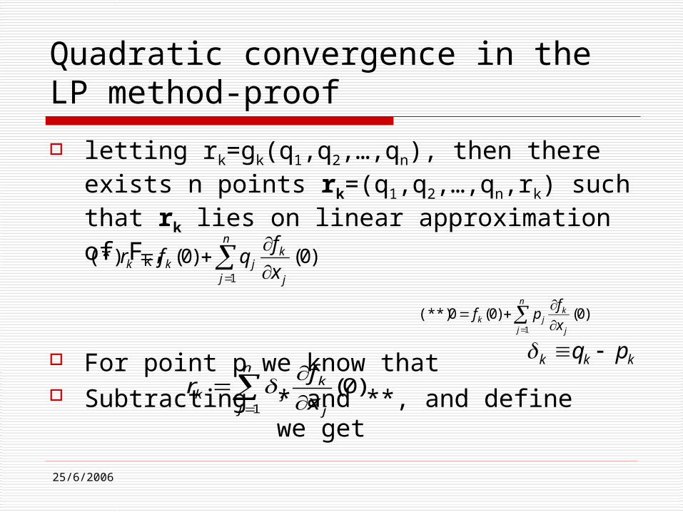
Quadratic convergence in the LP method-proof

letting rk=gk(q1,q2,…,qn), then there exists n points rk=(q1,q2,…,qn,rk) such that rk lies on linear approximation of Fk,

For point p we know that Subtracting * and **, and define

we get

n

j j

kjkk x

fqfr

1

)0()0( (*)

n

j j

kjk x

fpf

1

)0()0(0 (**)

kkk pq )0(

1

n

j j

kjk x

fr

25/6/2006

Quadratic convergence in the LP method-proof By Cramer’s rule we get ( assuming the

Jacobian matrix is non singular ) that where J is the Jacobian matrix , and Jk is the Jacobian matrix after exchanging k’th column with the column vector (r1,r2,…,rn)T

Since then and

since we get Then

J

J kk det

det

)(Ox

f

j

k )()det( nOJ

)( 2Ork )()det( 1 nk OJ

)( Ok

)0(1

n

j j

kjk x

fr

25/6/2006

Quadratic convergence in the LP method-proof q is chosen arbitrary and its distance from other

fixed point ( p ) is , then the distance between two points in the bounding box we want is also

Then the length of each side of the bounding box is also

The real size then ( in Rn ) is multiplied by factor of the bounding box ,then the dimensions of the new bounding box is

This hold for all K , then

)(O

)(O

)(O

)(O

)()()('' 2 OOOab kk

2'

25/6/2006

Subdivision with numerical improvements Subdivide the multivariate functions bounded within a

certain resolution Using the convex hull property if for a constrain Fi all

the control points have the same sign then it won’t have a roots.

For each cell with dimensions lower than the wanted resolution report for a root ( center of the cell )

Subdivision is terminated when it is known that there is an isolated root in the domain, in this case Newton-Raphson iterations is applied ( with quadratic convergence )

If the zero set has a dimension larger than 0, then fit a multivariate surface to the set of the discrete points found by means of least squares ( minimizing the L2 norm )

25/6/2006

Root Finding Algorithm

25/6/2006

Numerical improvement of the solution

for a given approximated solution u0 found , such that for each constrain Fi(u0)~0, using first order approximation, each graph Fi constrains the solution to be on the hyperplane which is defined in the point u0 as following : Consider the normal to the surface Fi(u) at the

point u0 :

Then the hyper plane at the point u0 is defined as

)(0 uPui

1,,...,,)(21

0m

iiii u

F

u

F

u

Fun

000 ),(),()(0 uunuunup iiui

25/6/2006

Numerical improvement of the solution

There are m such planes , and with the additional constraint that the component um+1=0, we end with n+1 linear equations( with m+1 variables)

If n=m then the system is full constrained and there is one solution

Otherwise if n < m a least square solution is found in an L2-norm ( finds the closest solution to u0 from the possible solutions set)

0)(0 upui

Uniqueness of a solution If it is known that there is a single solution

then it would be better to stop the subdivision and move to more efficient numerical procedure for root finding.

Definitions: Cone: normal cone of hypersurface Fi : set of all

possible normal vectors on Fi . Complementary (Tangent) cone:

2222cos,|),( vuvuuvC

niC

)90,(),(

0|ni

ni

ci

ni

ni

ni

ni

mci

vCC then vCC if

wu, that suchCuRwC

25/6/2006

Uniqueness of a solution Theorm:

Given m implicit hypersurfaces Fi(u)=0 . i=1,…m in Rm, there is at most one common solution if

Proof: Consider u0 (in Rm) is a common solution of the m

equations Fi(u)=0. Consider , from the relation we have

}0{1

ci

m

ic

)( 0uC ci

)(0)(| 0uCuFu cii

0011

)(0)(| uuCuFu ci

m

ii

m

i

25/6/2006

Examples Ray-Traps

Definition: Given a set of n planar curves, it’s ray-trap of length n is a set

of n points {Pi=Ci(ui)} such that a ray bouncing from Pi towards P(i+1)mod n will be reflected toward P(i+2)mod n

The incoming ray from Pi-1 and the outgoing ray towards Pi+1

should form an identical angle with the normal of Ci at Pi

This can be written as:

)(),()(

)()(

)(),()(

)()(

)(),()(

,,,

11

11

11

11

1

1

1

1

iiiiii

iiii

iiiiii

iiii

iiiiii

ii

iii

ii

iii

uxuyuN

as N take can we

uCuC

uNuCuC

uCuC

uNuCuC

orpp

Npp

pp

Npp

25/6/2006

Examples- ray-traps

25/6/2006

Examples Surface-Surface

Bisectors Let S1(u,v) and S2(u,v)

be two regular rational surfaces in R3 The points B=(x,y,z) on the bisector surface of S1 and S2

must satisfy the following constraints

,),(),,(),(),,(

.0),(

),,(

,0),(

),,(

,0),(

),,(

,0),(

),,(

2211

22

22

11

11

tsSBtsSBvuSBvuSB

dt

tsdStsSB

ds

tsdStsSB

dv

vudSvuSB

du

vudSvuSB

25/6/2006

Examples-Bisectors Let

Then we can choose and the problem is reduced to

v

vuS

u

vuSvun

),(),(),( 21

1

),(),( 11 vunvuSB

),(),(),,(),(),(

),(),(),,()),(),((2

,,,

0),(

,,,,

0),(

,,,,

21211

21121

2

2

tsSvuStsSvuSvun

tsSvuSvuntsSvuS

tsvu

where

t

tsStsvu

s

tsStsvu

25/6/2006

Examples-Bisectors

4 variables with 2 equations – under constrained problem

Can fit a bi-variate surface to discrete points sampled on the solution space.

25/6/2006

Examples-Bisectors

25/6/2006

Further improvements Preconditioning

Transformation of the system f=0 into equivalent system Mf=0 where M is nXn non singular matrix

global transformation Useful when two or more functions have closed

graphs on the domain, aims to increase the distance between them

The distance between two graphs is not trivial, so it is replaced by the distance between the vectors of the Bernstein basis coefficients

Local straightening: Interesting situation of reduction is when the

zero-set of the function fi are orthogonal to the xi direction

25/6/2006

Preconditioning-global transformation If then define the inner product between

functions

Let and let E be a matrix of unitary eigenvectors of Q. Then f’=Ef is a system of polynomials which are orthogonal for the inner product above.

Proof:

M

IMI

kIk uBbuf )()( ,

)(

M

I

jI

iIji bbff )()(,

njiji ffQ

,0

,

hpd) semiis Q ( Q of values eigen positive the are where

diagEQEEEffff

Qff

i

nTTTT

T

0

),...,,()')('( 21

25/6/2006

Preconditioning-global transformation

25/6/2006

Preconditioning- Local straightening

Local straightening

A better domain reduction can be done when the zero level of the functions fi are orthogonal to the xi axis.

This can be done by transforming the system f=0 in order to be closed to case (b). Transform locally the system into a system Jf-1(u0)f, where Jf is the Jacobian matrix of f at the point u0

njijif ufxuJ

,000 )()(

25/6/2006

Questions ???

Thanks

25/6/2006

Backup

25/6/2006

Improvements- Examples

25/6/2006

Further improvements - Reduction For a function f and j=1,…,n let

Then For any root u=(u1, u2 ,…, un) of the equation f(u)=0,

we have where t1/t2 is either a root of mj(f;uj)=0 or Mj(f;uj)=0 in [aj,bj]

or aj/bj if mj(f;uj)=0/ Mj(f;uj)=0 has no roots in [aj,bj] mj(f;uj)<=0<=Mj(f;uj)

j

j

j

jnkk

j

j

j

jnkk

d

ij

idiiijkdijj

d

ij

idiiijkdijj

uBbufM

uBbufm

0,...,,,0

0,...,,,0

)(max;

)(min;

21

21

);()();( jjjj ufMufufm

21 tut j

25/6/2006

Further improvements Reduction

Similar to the PP ( projected Polyhedron ) , reduce the domain of search

PP is based on the convex hull property The improvement consists in computing the

first/last root of the polynomial mj(fk,uj)/Mj(fk,uj) in the interval [aj,bj] and keep the intervals [t1,t2]

Analysis shows that with these improvements we get a quadratic convergence.