2.2 : 1/17

2.2 Common PDFs

•  uniform •  binomial •  Poisson •  normal (Gaussian) •  gamma •  analytical data

Uniform Density Function (1)

2.2 : 2/17

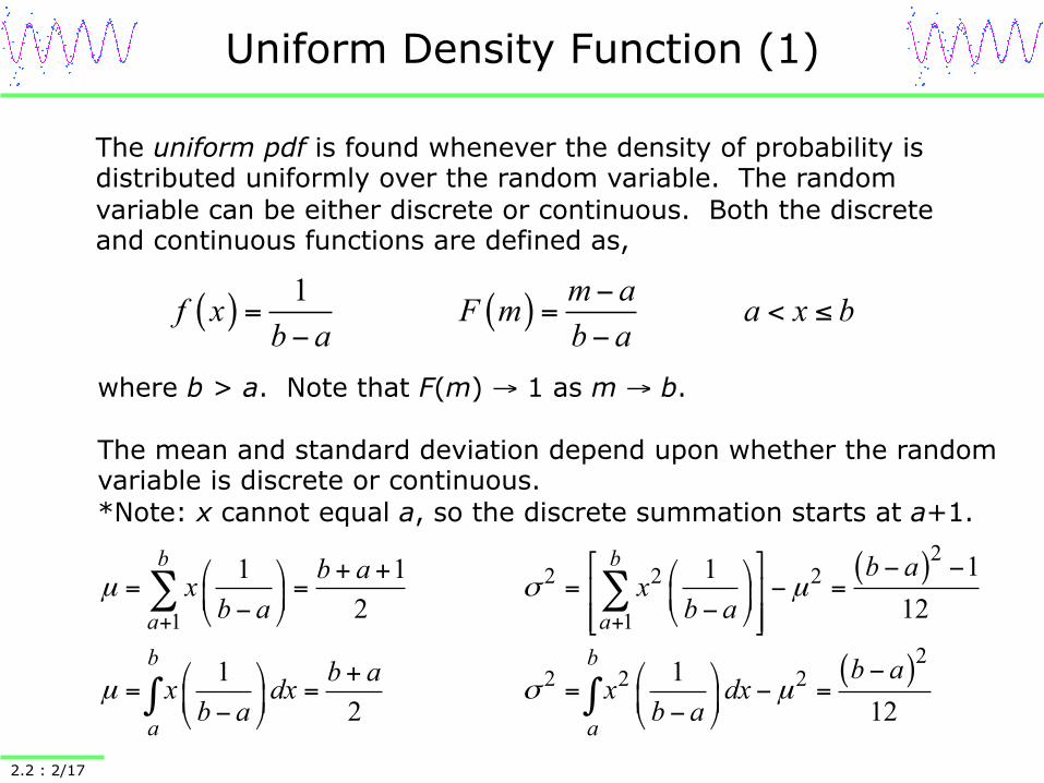
The uniform pdf is found whenever the density of probability is distributed uniformly over the random variable. The random variable can be either discrete or continuous. Both the discrete and continuous functions are defined as,

( ) ( )1 m af x F m a x bb a b a

−= = < ≤

− −

where b > a. Note that F(m) → 1 as m → b. The mean and standard deviation depend upon whether the random variable is discrete or continuous. *Note: x cannot equal a, so the discrete summation starts at a+1.

( )

( )

22 2 2

1 12

2 2 2

11 1 12 12

1 12 12

b b

a ab b

a a

b ab ax xb a b a

b ab ax dx x dxb a b a

µ σ µ

µ σ µ

+ +

⎡ ⎤ − −+ +⎛ ⎞ ⎛ ⎞= = = − =⎢ ⎥⎜ ⎟ ⎜ ⎟− −⎝ ⎠ ⎝ ⎠⎢ ⎥⎣ ⎦

−+⎛ ⎞ ⎛ ⎞= = = − =⎜ ⎟ ⎜ ⎟− −⎝ ⎠ ⎝ ⎠

∑ ∑

∫ ∫

Uniform Density Function (2)

2.2 : 3/17

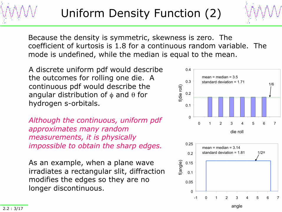
Because the density is symmetric, skewness is zero. The coefficient of kurtosis is 1.8 for a continuous random variable. The mode is undefined, while the median is equal to the mean.

0

0.1

0.2

0.3

0.4

0 1 2 3 4 5 6 7

die roll

f(die

roll)

mean = median = 3.5standard deviation = 1.71 1/6

0

0.05

0.1

0.15

0.2

0.25

-1 0 1 2 3 4 5 6 7

angle

f(ang

le)

mean = median = 3.14standard deviation = 1.81 1/2π

A discrete uniform pdf would describe the outcomes for rolling one die. A continuous pdf would describe the angular distribution of φ and θ for hydrogen s-orbitals. Although the continuous, uniform pdf approximates many random measurements, it is physically impossible to obtain the sharp edges. As an example, when a plane wave irradiates a rectangular slit, diffraction modifies the edges so they are no longer discontinuous.

Uniform Density Function (3)

2.2 : 4/17

A uniform random number generator is important because it is used to create random data following other pdfs. A uniform random number generator ranging from 0 to 1 can have edges with a slope of ±1015, which is a rather good approximation of infinity! In Mathcad there are two functions that generate uniformly distributed random numbers:

rnd(b) returns one continuous value over 0 ≤ x < b runif(N,a,b) returns an N-element vector of continuous values over a ≤ x < b

Example output of four sequentially generated values from rnd(1):

0.001268419437110 0.193323019891977 0.585006099194288 0.350308103486896

To simulate a die roll use, ceil(rnd(6)), where the ceiling function returns the next highest integer.

Binomial Density Function (1)

2.2 : 5/17

The binomial pdf is found whenever there are only two outcomes per experiment, and more than one experiment will be run. The two outcomes are called a success, S, or a failure, F. The resulting discrete random variable is the number of successes, x, for a given number of trials, n.

( )( )

( )( )0

! ! 0,1,2,! ! ! !

mx n x x n x

x

n nf x p q F m p q x nx n x x n x

− −

=

= = =− −∑ L

where p is the probability of a success and q = 1-p is the probability of a failure (many texts do not use q). The binomial theorem can be used to show that F(m) = 1 when m = n. The mean and the standard deviation are given by the following.

2np npq npqµ σ σ= = =

Since p and q are probabilities, they are unitless. The mean and standard deviation must have the same units as n. Since µ ∝ n and σ ∝ n1/2, x cannot have units.

Binomial Density Function (2)

2.2 : 6/17

Binomial skewness and kurtosis are given below. Skewness is positive for p < 0.5, zero when p = 0.5, and negative for p > 0.5.

( ) ( )23 4

23q p q p

npq nnpqα α

− −= = + −

Counter-current extraction follows the binomial pdf. A molecule partitioning into the mobile upper phase is a success, while partitioning into the stationary lower phase is a failure. Solutes with different values of p are distributed among the tubes differently.

freshupper

0 1 2 3

p p p p

q q q q

n = 1 n = 2 n = 3

Binomial Density Function (3)

2.2 : 7/17

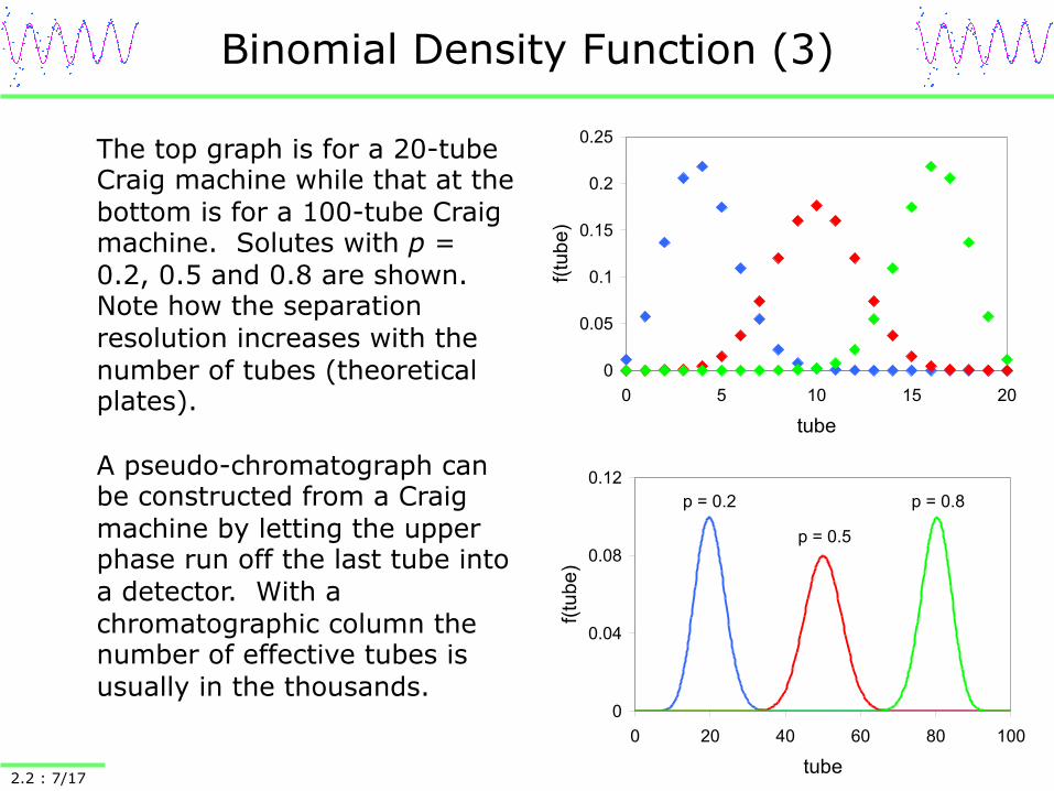
The top graph is for a 20-tube Craig machine while that at the bottom is for a 100-tube Craig machine. Solutes with p = 0.2, 0.5 and 0.8 are shown. Note how the separation resolution increases with the number of tubes (theoretical plates). A pseudo-chromatograph can be constructed from a Craig machine by letting the upper phase run off the last tube into a detector. With a chromatographic column the number of effective tubes is usually in the thousands.

0

0.05

0.1

0.15

0.2

0.25

0 5 10 15 20

tube

f(tube)

0

0.04

0.08

0.12

0 20 40 60 80 100

tube

f(tub

e)

p = 0.2

p = 0.5

p = 0.8

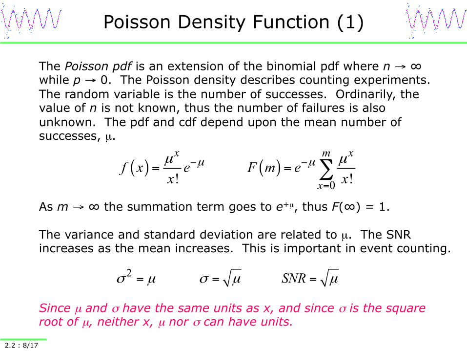
Poisson Density Function (1)

2.2 : 8/17

The Poisson pdf is an extension of the binomial pdf where n → ∞ while p → 0. The Poisson density describes counting experiments. The random variable is the number of successes. Ordinarily, the value of n is not known, thus the number of failures is also unknown. The pdf and cdf depend upon the mean number of successes, µ.

( ) ( )0! !

x xm

xf x e F m e

x xµ µµ µ− −

=

= = ∑

As m → ∞ the summation term goes to e+µ, thus F(∞) = 1. The variance and standard deviation are related to µ. The SNR increases as the mean increases. This is important in event counting.

2 SNRσ µ σ µ µ= = =

Since µ and σ have the same units as x, and since σ is the square root of µ, neither x, µ nor σ can have units.

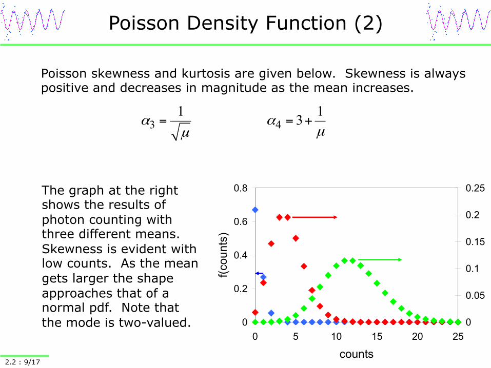
Poisson Density Function (2)

2.2 : 9/17

Poisson skewness and kurtosis are given below. Skewness is always positive and decreases in magnitude as the mean increases.

3 41 13α α

µµ= = +

The graph at the right shows the results of photon counting with three different means. Skewness is evident with low counts. As the mean gets larger the shape approaches that of a normal pdf. Note that the mode is two-valued. 0

0.2

0.4

0.6

0.8

0 5 10 15 20 25

counts

f(counts)

0

0.05

0.1

0.15

0.2

0.25

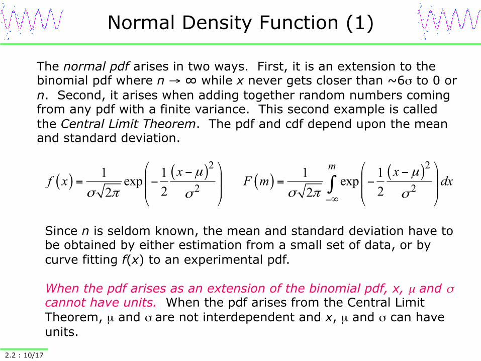
Normal Density Function (1)

2.2 : 10/17

The normal pdf arises in two ways. First, it is an extension to the binomial pdf where n → ∞ while x never gets closer than ~6σ to 0 or n. Second, it arises when adding together random numbers coming from any pdf with a finite variance. This second example is called the Central Limit Theorem. The pdf and cdf depend upon the mean and standard deviation.

( ) ( ) ( ) ( )2 2

2 21 1 1 1exp exp

2 22 2

mx xf x F m dx

µ µ

σ π σ πσ σ−∞

⎛ ⎞ ⎛ ⎞− −⎜ ⎟ ⎜ ⎟= − = −⎜ ⎟ ⎜ ⎟⎝ ⎠ ⎝ ⎠

∫

Since n is seldom known, the mean and standard deviation have to be obtained by either estimation from a small set of data, or by curve fitting f(x) to an experimental pdf. When the pdf arises as an extension of the binomial pdf, x, µ and σ cannot have units. When the pdf arises from the Central Limit Theorem, µ and σ are not interdependent and x, µ and σ can have units.

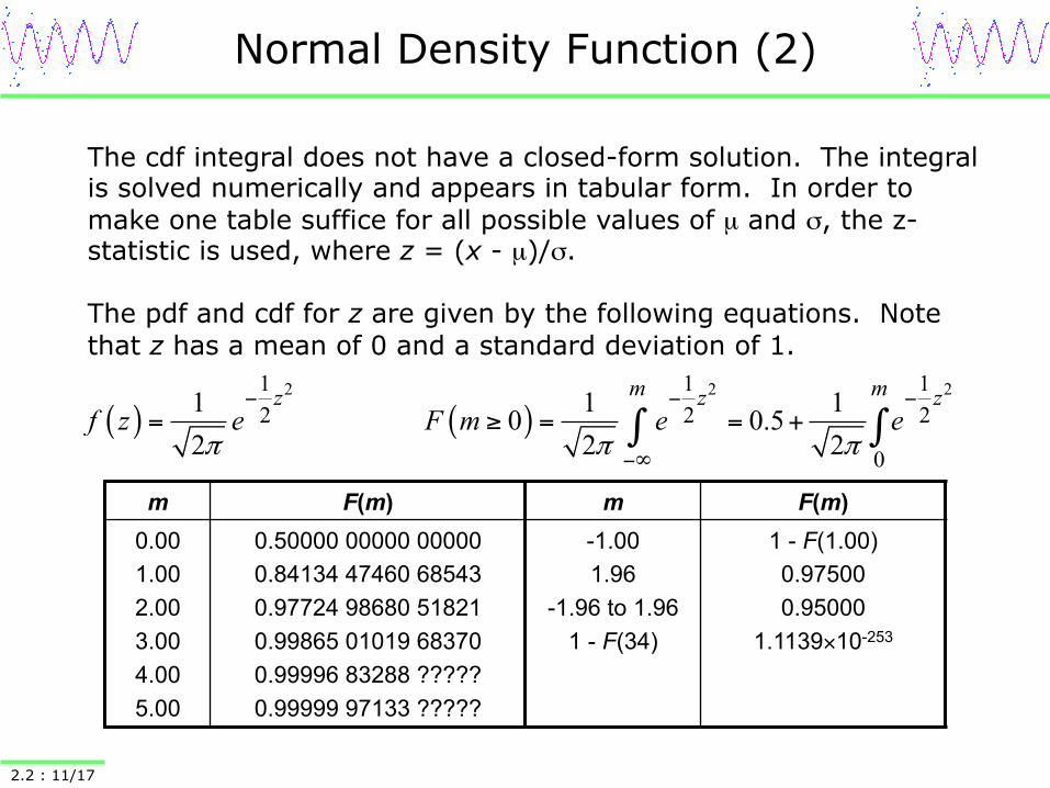
Normal Density Function (2)

2.2 : 11/17

The cdf integral does not have a closed-form solution. The integral is solved numerically and appears in tabular form. In order to make one table suffice for all possible values of µ and σ, the z-statistic is used, where z = (x - µ)/σ. The pdf and cdf for z are given by the following equations. Note that z has a mean of 0 and a standard deviation of 1.

( ) ( )2 2 21 1 1

2 2 2

0

1 1 10 0.52 2 2

m mz z zf z e F m e e

π π π

− − −

−∞

= ≥ = = +∫ ∫

m F(m) m F(m) 0.00 1.00 2.00 3.00 4.00 5.00

0.50000 00000 00000 0.84134 47460 68543 0.97724 98680 51821 0.99865 01019 68370 0.99996 83288 ????? 0.99999 97133 ?????

-1.00 1.96

-1.96 to 1.96 1 - F(34)

1 - F(1.00) 0.97500 0.95000

1.1139×10-253

Normal Density Function (3)

2.2 : 12/17

0

0.03

0.06

0.09

0 20 40 60 80 100

x

f(x)

Γ

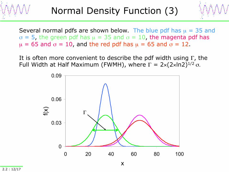
Several normal pdfs are shown below. The blue pdf has µ = 35 and σ = 5, the green pdf has µ = 35 and σ = 10, the magenta pdf has µ = 65 and σ = 10, and the red pdf has µ = 65 and σ = 12. It is often more convenient to describe the pdf width using Γ, the Full Width at Half Maximum (FWMH), where Γ = 2×(2×ln2)1/2 σ.

Gamma Density Function (1)

2.2 : 13/17

The continuous gamma density is usually associated with the square of normally distributed random variables and the sums of exponentially distributed random variables. The pdf depends upon an exponential constant, λ, and a power of the random variable, α, where α > 0 and λ > 0.

( )( )

1 xf x x eα

α λλα

− −=Γ

The gamma function (not density!), Γ(α), is obtained by numeric integration of the function at the right

( ) 1

0

xx e dxαα∞

− −Γ = ∫

It is possible to skip the numeric integration in many cases by knowing that Γ(1/2) = π1/2 and Γ(1) = 1, and using the recursive relationship, Γ(α+1) = αΓ(α) for α > 0. For positive integers this further reduces to Γ(α) = (α-1)!.

Gamma Density Function (2)

2.2 : 14/17

2 4 6 8 100

0.5

1

x0

f(x)

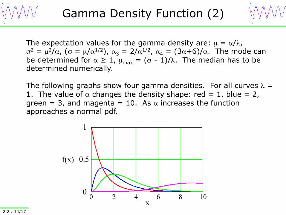
The expectation values for the gamma density are: µ = α/λ, σ2 = µ2/α, (σ = µ/α1/2), α3 = 2/α1/2, α4 = (3α+6)/α. The mode can be determined for α ≥ 1, µmax = (α - 1)/λ. The median has to be determined numerically. The following graphs show four gamma densities. For all curves λ = 1. The value of α changes the density shape: red = 1, blue = 2, green = 3, and magenta = 10. As α increases the function approaches a normal pdf.

Analytical Data as PDFs (1)

2.2: 15/17

Noise: It is commonly understood that noise on a measurement follows some specific pdf, which dictates SNE methods. Data: Many types of analytical procedures have outputs that are described by a pdf. This fact also affects SNE methods. Separations: The partitioning of molecules between two phases is determined by probability. Example - •  multiple extractions are used to separate an interference from the analyte •  goal #1 is to remove from the organic phase as many moles of analyte as possible •  goal #2 is to minimizing the number of moles of interferences removed •  this process is described by two cumulative distribution functions, one each for the analyte and interference

Analytical Data as PDFs (2)

2.2 : 16/17

If mass spectra are recorded at unit mass resolution, they can be described as discrete probability density functions. •  every time the analyte fragments, the specific bond being broken and the fragment picking up charge is determined by probability •  the parent population encompasses the range of physically possible masses •  the mass spectrum is obtained by performing a very large number of bond breaking and fragment forming events •  the more peaks occurring in a spectrum, the less probable it is to observe any one peak - thus the choice of ionization technique directly affects the sensitivity •  low resolution tandem mass spectrometry can be both sensitive and selective •  although mass spectrometry is untouchable for an ab initio identification at trace levels, the physics of ion production coupled with the fact that the data arise from a probability density function will prohibit much structural information at the single-molecule level

Analytical Data as PDFs (3)

2.2 : 17/17

A fluorescence spectrum is a continuous probability density function. In a double-monochrometer fluorimeter: •  emitted photons have random, but exact (Heisenberg-limited), wavelengths •  the spectrum is obtained by choosing the instrumental resolution, Δλ, and "binning" the emitted photons •  In a scanned instrument, one bin is used to collect data - the location of this bin is slowly moved across all wavelengths with the number of photons falling within the bin creating a pseudo-continuous spectrum. •  as Δλ is decreased, the resolution of the measurement is increased •  as Δλ is decreased fewer fluorescence photons will have the correct wavelength to pass through the monochromator to the detector, decreasing sensitivity •  Single-molecule detection has been achieved by measuring fluorescence. When using a single-channel detector, Δλ is made as large as possible to maximize the signal, reducing the selectivity. However, multi-channel detectors can recover some selectivity in single molecule spectroscopy.