Embed Size (px)
Citation preview

Page 1 of 13
10/19/2016
20XX-01-XXXX
The Effect of Swirl on the Flow Uniformity in Automotive Exhaust Catalysts
Author, co-author (Do NOT enter this information. It will be pulled from participant tab in
MyTechZone)
Affiliation (Do NOT enter this information. It will be pulled from participant tab in MyTechZone)
Abstract
In aftertreatment system design, flow uniformity is of paramount
importance as it affects aftertreatment device conversion efficiency
and durability. The major trend of downsizing engines using
turbochargers means the effect of the turbine residual swirl on the
flow needs to be considered. In this paper, this effect has been
investigated experimentally and numerically. A swirling flow rig
with a moving-block swirl generator was used to generate swirling
flow in a sudden expansion diffuser with a wash-coated diesel
oxidation catalyst (DOC) downstream. Hot-wire anemometry (HWA)
was used to measure the axial and tangential velocities of the swirling
flow upstream of the diffuser expansion and the axial velocity
downstream the monolith. With no swirl, the flow in the catalyst
monolith is highly non-uniform with maximum velocities near the
diffuser axis. At high swirl levels, the flow is also highly non-
uniform with the highest velocities near the diffuser wall. An
intermediate swirl level exists where the flow is most uniform. To
gain further insight into the mechanisms controlling flow
redistribution, numerical simulations have been performed using the
commercial CFD code STARCCM+. With no swirl, the central jet
transverses the diffuser, and a drastic flow redistribution takes place
near the monolith face due to its high resistance. Immediately
downstream of the sudden expansion, the flow separates from the
diffuser wall forming a separation zone around the central jet.
Increasing swirl reduces the size of this separation zone, and
eventually leads to the formation of the central recirculation zone
characteristic of high swirl flows. At intermediate swirl levels, the
size of the wall separation zone is reduced considerably, while the
axial adverse pressure gradient is insufficient to cause a central
recirculation. Such a flow regime occurs at relatively low swirl levels
(𝑆 ~ 0.23). This may have positive implications for aftertreatment
system design with low residual swirl levels from the turbine, which
might be tuned by adjusting the distance between the turbine and the
catalyst or employing guide vanes. The findings can be directly
transferred to other aftertreatment systems with a catalyst or
particulate filter. Moreover, swirling flows with an obstruction or a
high resistance device downstream (e.g. a heat exchanger or filter)
are present in many other applications such as cooling flows,
combustion and turbomachinery. Therefore the results are relevant to
a much wider research and industrial community.
Introduction
Catalytic converters are used in the automotive industry to comply
with increasingly stringent emissions regulations. Automotive
catalysts are monolith structures comprised of many parallel channels
of small hydraulic diameter ~ 1mm. Precious metals are applied to
the channel walls (as a thin washcoat) thus providing the high surface
area on which exhaust constituents can react. Optimum performance
requires that the residence time (or flow velocity) of the exhaust in
the monolith is the same for all channels. Indeed, the degree of flow
maldistribution across the monolith is often used as a criterion for
assessing the acceptability of a particular design.
The size of the monolith is largely dictated by engine capacity and
operating mode. Its length is normally kept as short as possible to
reduce pressure loss. A typical cylindrical monolith for a passenger
vehicle would have a diameter of around 100 mm and length around
150 mm. Space limitations often mean that short, wide-angled
diffusers are used to join the exhaust pipe to the front face of the
monolith. This results in flow separation within the diffuser and a
non-uniform flow distribution within the monolith.
Figure 1 shows a schematic of the flow field in an axisymmetric
catalyst assembly. Flow separates on entering the expander with the
resulting jet traversing the diffuser before rapidly spreading a short
distance upstream of the monolith. Part of the exhaust gas enters the
monolith channels, while some of it reverses to feed the large
recirculating vortices within the diffuser. The net result is that the
flow entering the monolith is maldistributed with the central channels
subject to higher velocity. Shorter residence time results in lower
conversion efficiency and can lead to high thermal loading and
premature deactivation [1]. Flow separation also produces higher
system pressure loss and increased fuel consumption [2].
Figure 1. Schematic of the flow field in a catalyst assembly.
To improve thermal efficiency and reduce carbon emissions,
automotive manufacturers are using downsized, turbo-charged
engines. This will have a knock-on effect on after-treatment systems
as the exhaust flow and temperature field will be modified by the
presence of the turbo-charger. In particular, the flow exiting the
turbocharger will have a significant swirl component depending on
engine operating conditions and turbocharger characteristics. The
brought to you by COREView metadata, citation and similar papers at core.ac.uk
provided by CURVE/open

Page 2 of 13
10/19/2016
effect of swirl on the flow field within the diffuser and the monolith
is largely unknown.
In simpler geometries, such as straight pipes and diffusers with no
flow restrictions downstream, the effect of swirl on the flow
distribution has been the subject of much fundamental and applied
research [3]-[10]. For wide-angle open diffusers, Okhio et al. [5]
have shown that increasing swirl number can suppress separation -
clearly of benefit for catalyst assemblies. However, high swirl can
lead to the development of very low pressures in the centre of the
vortex leading to flow reversal accompanied by a strong recirculating
zone within the diffuser and additional pressure loss [5]-[8]. Very
few studies exist of the effect of the downstream conditions on the
flow structure. These usually involve a flow constriction at a
considerable distance from the swirl generator which has been shown
to have a strong influence on the entire flow field [9]. In contrast, the
exhaust after-treatment assembly features a significant resistance,
namely the monolith, in close proximity to the diffuser outlet. The
authors are not aware of any flow studies which have been reported
for these situations. This paper presents an experimental and
numerical investigation of the flow distribution across an automotive
monolith as a function of swirl ratio and mass flow rate.
Experimental Study
Experimental setup
A schematic of the swirling flow rig is shown in Figure 2. The rig
features a swirl generator (2) - (4) placed upstream of an
axisymmetric catalyst assembly (6) - (7). The swirl generator is based
on the moving-block principle [12], a design that has been widely
used in gas turbine research. Its main advantage is its compactness
and the ability to easily adjust the swirl ratio.
Figure 2. Schematic of the swirling flow rig used in the study.
Air from a compressor is supplied to the test rig, with the flow rate
measured by a calibrated viscous flow meter (VFM) (1). Air enters
the plenum (2) before passing through a set of movable blocks that
can be positioned to generate varying levels of swirl by adjusting the
moveable plate (3). Air then enters the co-axial nozzle (4) and a
transparent annular extension piece (5). The transparent extension
piece (55 mm inner diameter with a 24 mm diameter annular insert)
provides access for the hot-wire anemometry (HWA) probe and a
thermocouple used for measurement of the axial and tangential
velocity components across the annulus. A sudden expansion diffuser
(6) connects the swirl generator assembly to the monolith (7) of
diameter, 𝐷 = 145.8 mm, followed by an outlet sleeve (8).
The sudden expansion diffuser ((6) in Figure 2) features inlet and
outlet diameters of 55 and 145.8 mm, respectively. A 50-mm-length,
55-mm-diameter inlet pipe connects the diffuser to the transparent
extension piece (5) of the swirl generator. The monolith was fitted
162 mm downstream from the expansion and is a cordierite, wash-
coated diesel oxidation catalyst (DOC) of 76.2-mm-length and 143.8-
mm-diameter with a nominal cell density of 400 cpsi.
Velocities across the annular transparent extension piece at the outlet
of the swirl generator as well as downstream of the monolith were
measured using a TSI IFA 300 constant temperature HWA system
with Dantec 55P11 single-normal (SN) HWA probes. Calibration of
the probes was performed using an automatic TSI 1129 calibration
rig with the probe stem and the hot wire both perpendicular to the
flow direction.
Velocity measurements across the annular transparent extension
piece were made with the HWA probe stem aligned with the y-axis
(Figure 3). Sampling of the analogue HWA signal was made at 200
Hz for a duration of 5 s. The probes are calibrated to measure the
velocity magnitude with the wire aligned perpendicular to the flow
direction. In the current configuration, the flow direction in the
annulus is not known a priori and varies with the probe y-position.
Therefore, a methodology has been developed in order to align the
probe with the mean flow vector at the various swirl intensities to
obtain the velocity magnitude.
To measure the flow profile in the annular section, the HWA probe
was traversed across the annulus radius at 1 mm intervals. At each
traversed position the probe was rotated around its axis and the signal
was recorded every 4° for 360° of total rotation. It was established
that a 4° rotation interval was sufficient to determine the flow
direction with required accuracy. The datum for the angular
positioning of the HWA probe can be chosen arbitrarily but has to be
set constant with respect to the rig geometry for all traversed
positions.
Figure 3. Schematic representation of HWA measurements made within the transparent annular extension.
A typical HWA response at one radial position is shown in Figure 4.
The least squares method is used to obtain the voltage maxima and
their angular positions. These correspond to the hot wire sensor being
perpendicular to the flow, therefore velocity magnitude and flow
direction can be obtained for each radial position inside the annulus.

Page 3 of 13
10/19/2016
Figure 4. HWA output with varying angular positioning of the probe within the annular transparent extension.
The datum point for the HWA sensor (when it is orthogonal to the x-
axis and lying in the xz-plane, see Figure 2) is determined by
adopting the above methodology for zero swirl flow. For non-zero
swirl flows, the angles obtained from the peaks of the HWA output
were subtracted from the datum angle, thus obtaining the actual flow
angle.
Positioning of the probe within the annular transparent extension was
accomplished through a custom-built probe positioning mechanism
(Figure 5). Radial positioning of the probe in the annular transparent
extension piece was achieved using combinations of 1- and 2-mm
aluminium spacers mounted along the probe support. Rotation of the
probe around its axis was achieved using a stepper motor-pulley
setup driven via an Arduino microcomputer interfaced to a custom-
built LabVIEW GUI.
Figure 5. HWA probe positioning mechanism for angular and radial traverse
of the HWA probe.
Velocity profiles downstream of the DOC were measured using a SN
HWA probe with the probe stem aligned parallel to the mean flow
direction. The probe was calibrated with the probe stem parallel to
the axis of the calibration nozzle, and the analogue HWA signal was
sampled at 1 kHz for a duration of 1 s. A two-axis programmable
traverse system was used to traverse the HWA probe along the two
diameters of the outlet sleeve (horizontal and vertical). Measurements
were made 30 mm downstream of the monolith outlet. At this
distance the jets exiting the monolith from adjacent channels will
have mixed sufficiently to provide smooth radial profiles at the rear
of the monolith.
Pressure tappings along the diffuser wall allowed measurement of the
wall pressure distribution using water manometers. More tappings
were used around the expansion point and just upstream of the DOC
where the highest pressure variation was expected to occur.
Two mass flow rates were considered, 63 and 100 g/s, which are
typical of 2.5-l engines operating at full load between 2500-4000 rpm
at 100% volumetric efficiency. The swirl intensity was varied by
adjusting the angle of the moveable plate of the swirl generator from
0° (no swirl) to 18° (high swirl).
Results
In order to characterise the level of swirl, a non-dimensional swirl
number, 𝑆, can be defined as
𝑆 =𝐺𝜃
𝐺𝑥𝑟0, (1)
where the swirl and axial momentum fluxes, 𝐺θ and 𝐺𝑥, are given by
𝐺θ = ∫ 𝜌𝑈𝑊𝑟𝑟𝑜
𝑟𝑖2𝜋𝑟𝑑𝑟 (2)
𝐺𝑥 = ∫ 𝜌𝑈2𝑟𝑜
𝑟𝑖2𝜋𝑟𝑑𝑟 (3)
In Eqs. (2) and (3), 𝜌 is the air density, 𝑈 is the axial velocity
component, 𝑊 is the tangential velocity component, and 𝑟 is the
radial distance from the centre of the annular cross-section of 𝑟𝑜 and
𝑟𝑖 outer and inner radii, respectively (Figure 3). The swirl number
values estimated from the velocity measurements at the exit from
swirl generator are shown in Table 1.
Figure 6 and Figure 7 show the axial and tangential velocity profiles
in the annulus upstream of the expansion, normalised using the mean
axial velocity. Here, the non-dimensionalised distance across the
annulus is defined as 𝑑 = (𝑟 − 𝑟𝑖) (𝑟𝑜 − 𝑟𝑖)⁄ .
The velocity profiles at zero swirl and 𝑆 = 0.23/0.26 are very similar
for both mass flow rates, with some variation near the walls. At the
higher swirl rates, the effects of swirl on the axial velocity profiles
becomes more apparent. Velocities closer to the annulus inner wall
are lower than those for no swirl and low swirl flow conditions. At
the highest swirl level considered a significant amount of flow is
directed towards the outer wall causing the axial velocities to peak at
around 𝑑 = 0.8 from the annulus inner wall.
The effect of swirl on the tangential velocity profiles is shown in
Figure 7. At low swirl levels, the tangential velocity increases
towards the outer wall of the annulus. As swirl is increased, the peak
in the tangential velocity profile gradually gets closer to the inner
wall of the annulus. At the highest swirl, where maximum velocities
appear 1/3 of the way from the annulus inner wall, a typical Rankine
vortex flow pattern is observed.
Changes in the mass flow rates do not appear to significantly affect
the flow pattern for any of the swirl levels considered.
In order to check the accuracy of the flow measurements in the
annulus, the air mass flow rate was calculated from the HWA axial
velocity measurements. A good agreement with the mass flow rate
measurements from the VFM was obtained, thus validating the
methodology (Table 2).
1.2
1.3
1.4
1.5
1.6
0 60 120 180 240 300 360
Volt
age
(V)
Angle of rotation of HWA probe (°)
HWA Voltage Least squares fit
Page 4 of 13
10/19/2016
Table 1. Estimated swirl number values
Swirl number, 𝑺
(experiments)
Swirl number,
𝑺 (simulation)
Swirl generator angle 63 g/s 100 g/s 63 g/s
4° (low swirl) 0.23 0.26 0.25
7° (intermediate swirl) 0.44 0.45 0.47
10° (intermediate swirl) 0.70 0.63 0.69
18° (high swirl) 1.65 1.63 1.42
Figure 6. Normalised axial velocity profiles across annulus of swirl
generator outlet. Filled and non-filled markers indicate measurements at 100
and 63 g/s, respectively.
Figure 7. Normalised tangential velocity profiles across the annulus of the swirl generator outlet.
Table 2 The difference between mass flow rate measurements from VFM
and calculated mass flow rates from HWA data. HWA1 refers to HWA measurements at the swirl generator exit, HWA2 refers to HWA
measurements downstream of the catalyst.
Swirl generator angle
Error (%)
calculated using
HWA1
Error (%)
calculated using
HWA2
63 g/s 100 g/s 63 g/s 100 g/s
0° (no swirl) -4.3 -6.4 -0.8 -4.6
4° (low swirl) -4.8 -10.1 0.5 -2.5
7° (intermediate swirl) -7.1 -11.2 -0.8 -1.2
10° (intermediate swirl) -8.2 -8.0 7.4 3.5
18° (high swirl) -8.8 -13.4 17.6 18.5
Figure 8 shows the velocity profiles measured along two diameters
and demonstrates the flow is approximately axisymmetric in the
monolith. As the flow was determined to be axisymmetric, the
averages of the two traverse directions are presented in Figure 8 for
all flow conditions.
With no swirl the velocity profiles exhibit a peak on the axis of the
DOC where the jet from the inlet pipe enters the monolith. However,
high resistance presented by the monolith causes the jet to spread
outwards towards the diffuser outer wall. This causes the pressure to
rise in the outermost regions of the diffuser wall forcing flow through
this region resulting in the secondary peaks in the velocity profile.
At low swirl (swirl generator angle of 4) the velocities are relatively
flat for both mass flow rates. Due to radial pressure gradients induced
by the swirling motion, more of the flow is directed towards the
diffuser wall, resulting in higher velocities in the outer region of
diffuser.
With further increase in swirl, the velocity magnitude near the wall
continues to rise. At the intermediate swirl level (swirl generator
angle of 7) the normalised axial velocity near the wall is almost
eight times higher than that in the centre. At the same time, an
adverse axial pressure gradient starts to develop near the axis of the
assembly causing a "dip" in the velocity profile.
At swirl generator angle of 10 and 18 the onset of reversed flow is
observed in the centre of the diffuser. Note that hot wire anemometry
only measures velocity magnitude, therefore the reverse flow appears
as another peak at the centre of the diffuser. This is the reason for
high mass flow rate calculation error (Table 2) for high swirl levels.
The direction of the flow for 10 and 18 swirl generator angles was
checked in a previous study using a shielded probe [13], and it was
confirmed that the velocities in the middle of the diffuser were indeed
negative.
The effect of the change in mass flow rate from 63 g/s to 100 g/s is
insignificant, and the flow structure is clearly dominated by swirl.
0.0
0.2
0.4
0.6
0.8
1.0
1.2
0.0 0.2 0.4 0.6 0.8 1.0
U/U
m
d
Mass flow 63 g/s, S = 0 Mass flow 100 g/s, S = 0
Mass flow 63 g/s, S = 0.23 Mass flow 100 g/s, S = 0.26
Mass flow 63 g/s, S = 0.44 Mass flow 100 g/s, S = 0.45
Mass flow 63 g/s, S = 0.70 Mass flow 100 g/s, S = 0.63
Mass flow 63 g/s, S = 1.65 Mass flow 100 g/s, S = 1.63
0.0
0.5
1.0
1.5
2.0
2.5
0 0.2 0.4 0.6 0.8 1
W/U
m
d
Mass flow 63 g/s, S = 0.23 Mass flow 100 g/s, S = 0.26
Mass flow 63 g/s, S = 0.44 Mass flow 100 g/s, S = 0.45
Mass flow 63 g/s, S = 0.70 Mass flow 100 g/s, S = 0.63
Mass flow 63 g/s, S = 1.65 Mass flow 100 g/s, S = 1.63

Page 5 of 13
10/19/2016
Figure 8. Normalised velocity profiles 30 mm downstream of the DOC
where D is the diameter of the outlet sleeve and r is the distance from the axis.
Since flow uniformity is an important factor in catalyst design, it is
instructive to introduce the flow maldistribution index, 𝑀, in the
monolith [2]:
𝑀 =(Peak velocity−Mean velocity)
Mean velocity (4)
In Eq. (4) the peak and mean velocities refer to the highest and
average velocity magnitudes, respectively, obtained from HWA
measurements across the outlet sleeve for any particular swirl
number.
Table 3 shows the maldistribution index for all experimental
conditions. Maldistribution is lowest at low swirl levels. For all swirl
levels, the maldistribution increases with flow rate, a characteristic
that has been reported previously in the literature [14, 15].
Another parameter used to assess flow uniformity is flow distribution
index/flow uniformity index [16] defined as
total
ii
AU
AUU
25.01
(5)
where �̅� is the mean velocity, 𝑈𝑖 are measured velocities, 𝐴𝑖 are
corresponding annular segment areas and 𝐴𝑡𝑜𝑡𝑎𝑙 is the total area of
the annulus cross-section. The value of 𝛾 = 1 corresponds to fully
uniform flow.
The flow uniformity index shown in Table 3 confirms the fact that
low swirl level (𝑆 0.23) provides most uniform flow.
Table 3. Maldistribution index at different flow conditions.
Swirl generator angle
Maldistribution
index, 𝑴
Flow uniformity
index,
63 g/s 100 g/s 63 g/s 100 g/s
0° (no swirl) 0.69 0.83 0.86 0.83
4° (low swirl) 0.40 0.48 0.96 0.94
7° (intermediate swirl) 0.76 1.02 0.91 0.88
10° (intermediate swirl) 1.13 1.29 0.87 0.85
18° (high swirl) 1.37 1.39 0.79 0.78
CFD Modelling
In order to gain insight into the flow structure within the diffuser
CFD simulations have been performed for a mass flow rate of 63 g/s.
Model setup
The commercial CFD code StarCCM+ was used to model the flow. It
is known that inlet conditions have a significant effect on the
simulation results [17]. Therefore the full assembly together with
swirl generator was considered. The geometry is shown in Figure 9.
It includes the swirl generator (2-4 in Figure 2), extension piece (5 in
Figure 2), diffuser (6 in Figure 2), monolith (7 in Figure 2) and the
outlet sleeve (8 in Figure 2). As the swirl generator has 8 identical
blocks spread azimuthally [10], a 45-degree wedge is used with
periodic boundaries on each side.
A polyhedral mesh was used in all calculations. Ten prism layers
were added at the walls, inlet and outlet boundaries in order to
capture high gradients normal to these surfaces. Turbulence was
modelled using the Reynolds-averaged Navier-Stokes (RANS) 𝑣2𝑓
model, which is known to perform well in separating flows [18]. A
two-layer low Reynolds number wall treatment was used with 𝑦+ < 5
in all simulations. A mesh independence study was performed for
each swirl levels, resulting in five grids comprising 2 - 2.1M cells
each. All simulations were performed using the SIMPLE algorithm.
The equations were discretised using a second-order upwind scheme.
Uniform velocity, 1% turbulence intensity and turbulent viscosity
ratio of 10 were specified at the swirl generator inlet. A constant
pressure condition (𝑝 = 0) was used at the outlet. Periodic boundaries
were specified at the side surfaces, and non-slip conditions were
applied at the walls.
The flow in the monolith was modelled using a porous medium
approach, where the monolith with parallel flow channels is modelled
as a porous medium that resists the flow. Thus individual channels
are not modelled which reduces meshing and computational time
[19]. The resistance coefficients were estimated from experimental
data obtained under cold flow conditions [13] using a correlation
uuuLp α/ . Here p is pressure drop, 𝑢 is superficial
velocity, L is the monolith length, = 684.37 kg/m3s and = 28.28
kg/m4 are viscous and inertial resistance coefficients, respectively.
The resistance coefficients (both viscous and inertial) in the y and z
directions were set to 105 to ensure that the flow in the monolith is
unidirectional.
Additional resistance is introduced in the monolith due to the oblique
entrance of the flow into the channels [20]. This was implemented in
the model as a momentum source term ∆𝑝𝑜𝑏𝑙𝑖𝑞𝑢𝑒 = ±𝜌𝑣2/2, where
𝜌 is the air density and 𝑣 is velocity tangential to the monolith front
face at a distance 1 mm from the front face of the monolith. The sign
is chosen so that the resultant force opposes the flow.
0.0
0.5
1.0
1.5
2.0
2.5
-0.5 -0.3 -0.1 0.1 0.3 0.5
U/U
m
r/D
Mass flow 63 g/s, S = 0 Mass flow 100 g/s, S = 0
Mass flow 63 g/s, S = 0.23 Mass flow 100 g/s, S = 0.26
Mass flow 63 g/s, S = 0.44 Mass flow 100 g/s, S = 0.45
Mass flow 63 g/s, S = 0.70 Mass flow 100 g/s, S = 0.63
Mass flow 63 g/s, S = 1.65 Mass flow 100 g/s, S = 1.63

Page 6 of 13
10/19/2016
(a)
(b)
(c) Figure 9. Geometry and mesh used in simulations: no swirl (a), 7° (b) and
18° (c) swirl generator angles.
Inlet conditions
Setting inlet conditions for swirling flows is a non-trivial task.
Previous research has shown that in many swirling flow
configurations the flow features are often closely coupled to and
affect the flow upstream [17]. Therefore, prescribing the flow
immediately upstream of the test section may cause unphysical flow
behaviour, and also result in suppressing some of the flow features.
This was observed in preliminary modelling in this study, and
including the whole swirl generator assembly has been used to
address this issue.
Comparison between simulation results and hot wire measurements at
the outlet of the swirl generator (Figure 10 and Figure 11) shows a
very good agreement in the axial velocities for all swirl levels.
Tangential velocity distribution is not predicted as well (Figure 11).
For the highest swirl (𝑆 = 1.65), simulation results show swirl levels
characteristic to solid body rotation, while the experimental
measurements have a swirling component maximum near the inner
wall of the annular section. This could be a deficiency in the
turbulence model which assumes isotropic turbulence even under
swirling conditions.
The values of swirl number are shown in Table 1 and are in
reasonable agreement with the experimental ones, apart from the
highest swirl case where the swirl level is underpredicted upstream of
the assembly as shown in Figure 11. The results show that CFD still
captures most of the important features of the flow, which will be
discussed below. Therefore, it can be argued that the level of swirl
upstream is more important than the exact swirl velocity profile.
As shown previously, for all swirl levels the flow in the diffuser,
monolith and outlet sleeve is nearly axisymmetric, therefore only one
azimuthal cross-section is considered. For convenience, the values of
swirl numbers calculated from the experiments will be used in
discussing both experimental and simulation results.
No swirl (𝑺 = 0)
The flow structure and pressure distribution in the diffuser for 𝑆 = 0
is shown in Figure 12. A small recirculation zone is formed behind
the solid insert in the swirl generator outlet. A large recirculation
zone is formed in the main body of the diffuser, away from the
central jet. This separation zone extends along the whole side wall of
the diffuser.
When the central annular jet reaches the monolith, high resistance of
the monolith channels causes the flow to slow down, and the jet
spreads towards the wall of the diffuser. Therefore there is dramatic
flow redistribution just upstream of the monolith. A high pressure
area is observed at the front face of the monolith where the flow
decelerates. When the diverted flow reaches the wall, the pressure
rises with some of the flow entering the monolith near the wall, and
the remainder feeding the diffuser vortex. This causes a secondary
axial velocity peak near the wall (Figure 13).
The pressure coefficient, 𝑐𝑝, is defined as
25.0 U
ppc p
, (6)
where 𝜌 is air density, p is wall static pressure at the measurement
location, p is the atmospheric pressure and U the average axial
velocity in the annular section.
Pressure along the wall of the diffuser (Figure 14) is nearly constant,
increasing just upstream of the monolith. A stagnation point is
present at the diffuser wall where the separation zone ends, and a
pressure maximum is observed. The trend in predicted pressure
matches well with experiment.

Page 7 of 13
10/19/2016
Figure 10. Normalised axial velocity: comparison between experiment and simulations for 63 g/s mass flow within the annulus.
Figure 11. Normalised tangential velocity: comparison between experiment
and simulations for 63 g/s mass flow within the annulus.
Figure 12. Pressure coefficient distribution, streamlines and normalised
velocity vectors, 𝑆 = 0. Velocity is normalised by mean inlet axial velocity.
Figure 13. Velocity distribution 30 mm downstream of the monolith
(normalised by the mean velocity in the same cross-section) for 𝑆 = 0 and 𝑆 = 0.23, 63 g/s.
Figure 14. Pressure coefficient along the diffuser wall for 𝑆 = 0, 63 g/s.
Figure 15. Pressure coefficient distribution, constrained streamlines and
normalised velocity vectors, 𝑆 = 0.23. Velocity is normalised by mean inlet axial velocity.
0.0
0.2
0.4
0.6
0.8
1.0
1.2
1.4
0.0 0.2 0.4 0.6 0.8 1.0
U/U
m
d
Experiment (S = 0) Simulation (S = 0)Experiment (S = 0.23) Simulation (S = 0.25)Experiment (S = 0.44) Simulation (S = 0.47)Experiment (S = 0.70) Simulation (S = 0.69)Experiment (S = 1.65) Simulation (S = 1.42)
0.0
0.5
1.0
1.5
2.0
2.5
0.0 0.2 0.4 0.6 0.8 1.0
W/U
m
d
Experiment (S = 0.23) Simulation (S = 0.25)
Experiment (S = 0.44) Simulation (S = 0.47)
Experiment (S = 0.70) Simulation (S = 0.69)
Experiment (S = 1.65) Simulation (S = 1.42)
0.0
0.5
1.0
1.5
2.0
2.5
0.0 0.1 0.2 0.3 0.4 0.5
U/U
m
r/D
Experiment (S = 0) Simulation (S = 0)
Experiment (S = 0.23) Simulation (S = 0.25)
0.0
0.1
0.2
0.3
0.4
0.5
-80 -40 0 40 80 120 160
Cp
Distance from expansion (mm)
Experiment (S = 0) Simulation (S = 0)

Page 8 of 13
10/19/2016
Figure 16. Pressure coefficient along the diffuser wall for 𝑆 = 0.23, 63 g/s.
The flow downstream of the monolith (Figure 13) is mostly
unidirectional with two velocity peaks: primary velocity peak in the
middle and secondary velocity peak near the walls. The model
underpredicts flow maldistribution in the monolith but captures the
trend reasonably well.
Low swirl (S = 0.23)
Introduction of a swirling velocity component causes an increase in
radial pressure gradients, and higher axial flow near the wall of the
diffuser as a result (Figure 13). The trade-off between the inertia and
centrifugal forces causes the nearly flat profile observed in the
experiments, with slight peaks near the wall. The simulation correctly
predicts the trend of the flow becoming more uniform with increasing
swirl level, however it still shows a degree of non-uniformity
throughout the cross-section. This may be caused by the slight
underprediction of the inlet swirl levels as shown in Figure 11.
Figure 15 shows that the separation zone downstream of the sudden
expansion still covers the whole diffuser wall. The pressure is
noticeably lower along the diffuser axis, and the separation zone
behind the annular insert becomes larger. The high pressure area at
the monolith front face, where the jet slows down, has moved further
towards the wall.
Pressure coefficient variation at the wall (Figure 16) also differs
considerably between CFD and experimental results. Much better
pressure recovery is observed in the experiment, without the steep
gradient near the monolith front face.
Intermediate swirl (𝑺 = 0.44)
At swirl levels higher than 0.23, further increase of the separation
zone size behind the annulus is predicted (Figure 17). In contrast, the
separation zone at the sudden expansion shrinks considerably, and a
pressure maximum at the wall marks the point of reattachment where
the swirling jet reaches the wall (Figure 18). The general pressure
distribution trend and the position of the reattachment point is
predicted reasonably well, however CFD results exhibit much more
pronounced pressure variation along the wall. In contrast to the low
swirl case, the adverse pressure gradient on the centre line is capable
of producing reverse flow.
Downstream of the catalyst, the velocity features a pronounced peak
near the wall characteristic to swirling flows (Figure 19).
Experimental and CFD results agree well, with CFD missing the
"flat" part of the velocity profile around 𝑟/𝐷 = 0.25 and
overpredicting the velocity magnitude in the centre.
Figure 17. Pressure coefficient distribution, constrained streamlines and
normalised velocity vectors, 𝑆 = 0.44. Velocity is normalised by mean inlet axial velocity.
Figure 18. Pressure coefficient along the diffuser wall for 𝑆 = 0.44, 63 g/s.
Figure 19. Velocity distribution 30 mm downstream of the monolith
(normalised by the mean velocity in the same cross-section) for 𝑆 = 0.44, 63 g/s.
Swirl levels (𝑺 = 0.70 and 𝑺 = 1.65)
Increasing swirl further results in the adverse pressure gradients near
the axis so high that the central recirculation zone now stretches all
the way through the catalyst (Figure 20, Figure 21). It causes reverse
flow near the axis of the monolith and further downstream. This is a
well-known feature of highly swirling flows, when high radial
pressure gradients induced by swirl result in adverse axial pressure
gradients along the axis of the assembly.
-0.1
0.0
0.1
0.2
0.3
0.4
0.5
0.6
0.7
0.8
-80 -40 0 40 80 120 160
Cp
Distance from expansion (mm)
Experiment (S = 0.23) Simulation (S = 0.25)
-0.1
0.0
0.1
0.2
0.3
0.4
0.5
0.6
0.7
0.8
-80 -40 0 40 80 120 160
Cp
Distance from expansion (mm)
Experiment (S = 0.44) Simulation (S = 0.47)
0.0
0.2
0.4
0.6
0.8
1.0
1.2
1.4
1.6
0.0 0.1 0.2 0.3 0.4 0.5
U/U
m
r/D
Experiment (S = 0.44) Simulation (S = 0.47)
Page 9 of 13
10/19/2016
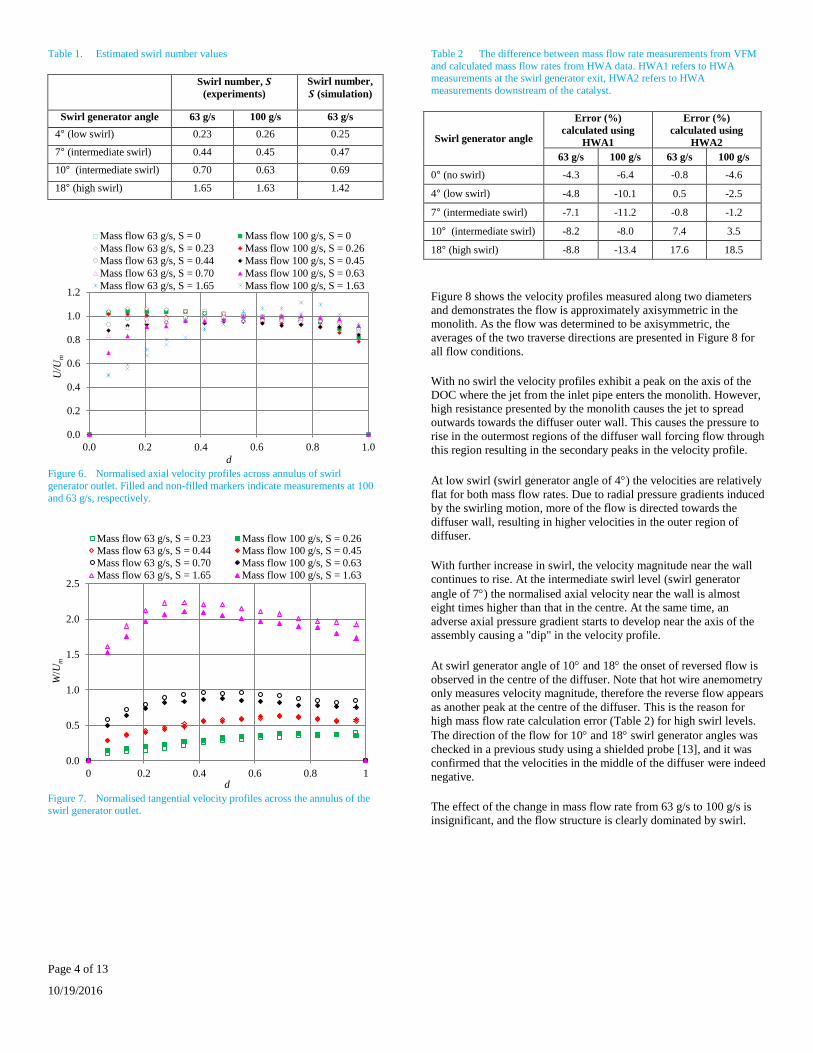
Thus, the axial velocity downstream of the monolith features a
maximum near the walls and reverse flow near the axis of the
assembly (Figure 22, Figure 23). Comparison with experimental
measurements shows a reasonable agreement with the hot wire
velocity measurements. Simulations underpredict velocity variation,
with velocity maxima and minima magnitudes lower than those
observed in experiments for the highest swirl level. The apparent
underprediction of the minimum velocity is due to the inability of
HWA to detect reverse flow. Hot-wire anemometry only measures
the magnitude of the velocity, thus the velocities are shown as
positive where reverse flow is observed near the axis of the assembly.
The separation zones in the diffuser corners shrink further so that the
(high-pressure) stagnation point where the jet meets the wall is
shifted toward the corner (Figure 24, Figure 25). It is expected that at
higher swirl levels the separation zones will disappear completely.
Figure 20. Pressure coefficient distribution, constrained streamlines and
normalised velocity vectors, 𝑆 = 0.7. Velocity is normalised by mean inlet axial velocity.
Figure 21. Pressure coefficient distribution, constrained streamlines and
normalised velocity vectors, 𝑆 = 1.65. Velocity is normalised by mean inlet
axial velocity.
Figure 22. Velocity distribution 30 mm downstream of the monolith
(normalised by the mean velocity in the same cross-section) for 𝑆 = 0.70, 63 g/s.
Figure 23. Velocity distribution 30 mm downstream of the monolith
(normalised by the mean velocity in the same cross-section) for 𝑆 = 1.65, 63 g/s.
Figure 24. Pressure coefficient along the diffuser wall for 𝑆 = 0.70, 63 g/s.
Figure 25. Pressure coefficient along the diffuser wall for 𝑆 = 1.65, 63 g/s.
Conclusion
The effect of swirl on flow uniformity in a catalyst has been
investigated experimentally and numerically. The results confirm that
an optimal swirl level exists where the flow in the catalyst is most
uniform with the maldistribution index of 0.4. This flow regime
occurs when the inertial force driving the central jet in the diffuser is
balanced by the centrifugal force forcing the flow to redistribute
towards the diffuser wall. It happens for relatively low swirl levels (𝑆
~ 0.23).
0.0
0.2
0.4
0.6
0.8
1.0
1.2
1.4
1.6
1.8
0.0 0.1 0.2 0.3 0.4 0.5
U/U
m
r/D
Experiment (S = 0.70) Simulation (S = 0.69)
0.0
0.5
1.0
1.5
2.0
2.5
0.0 0.1 0.2 0.3 0.4 0.5
U/U
m
r/D
Experiment (S = 1.65) Simulation (S = 1.42)
-0.2
0.0
0.2
0.4
0.6
0.8
1.0
1.2
1.4
-80 -40 0 40 80 120 160
Cp
Distance from expansion (mm)
Experiment (S = 0.70) Simulation (S = 0.69)
0.0
1.0
2.0
3.0
4.0
5.0
-80 -40 0 40 80 120 160
Cp
Distance from expansion (mm)
Experiment (S = 1.65) Simulation (S = 1.42)
Page 10 of 13
10/19/2016
CFD simulations demonstrate that a simple RANS-based
methodology is sufficient to get an insight into the main flow features
and mechanisms governing flow redistribution depending on swirl.
Velocity profiles downstream of the catalyst are predicted well, while
pressure variation at the diffuser wall is generally overpredicted. The
results also indicate that the most uniform flow regime is predicted to
occur at higher swirl levels, compared to experiment.
In general, a RANS-based CFD model has predicted the most
important flow features at lower and higher swirl levels reasonably
well. However, the model fails to correctly predict the flow regime
where the flow changes from a central jet dominated pattern to the
wall jet dominated pattern. This is attributed to the fact that the flow
distribution is very sensitive to the swirl levels upstream of the
assembly, and these are not predicted with sufficient accuracy by
RANS. Moreover, the delicate balance between the opposing forces
dominating the central jet and the wall jet regimes in the diffuser is
affected by the intrinsic anisotropy of the flow turbulence. Thus, the
isotropic 𝑣2𝑓 model is not suitable for exploring this flow regime.
Using anisotropic turbulence models, such as a Reynolds Stress
Turbulence model or the more complex Large Eddy Simulation
models are needed for improving flow predictions. This is subject of
ongoing work.
The findings can be used in the design of aftertreatment devices (e.g.
catalysts and filters), where swirl levels could be adjusted by
optimising the aftertreatment system geometry downstream of the
turbocharger.
References
1. Martin, A. P., Will, N. S., Bordet, A., Cornet, P. et al., "Effect of
Flow Distribution on Emissions Performance of Catalytic
Converters," SAE Technical Paper 980936, 1998, doi:
10.4271/980936.
2. Wendland, D. W., Sorrell, P. L. and Kreucher, J. E., "Sources of
Monolith Catalytic Converter Pressure Loss," SAE Technical
Paper 912372, 1991, doi: 10.4271/912372.
3. So, K. L., "Vortex Phenomena in a Conical Diffuser," AIAA J.
5(6):1062-1078, 1967, doi: 10.2514/3.4139.
4. Clausen, P. D., Koh, S. G. and Wood, D. H., "Measurements of a
Swirling Turbulent Boundary Layer Developing in a Conical
Diffuser," Exp Therm Fluid Sci. 6(1):39-48, 1993, doi:
10.1016/0894-1777(93)90039-L.
5. Okhio, C. B., Horton, H. P. and Langer, G., "Effects of Swirl on
Flow Separation and Performance of Wide Angle Diffusers," Int
J Heat Fluid Fl. 4(4):199-206, 1983, doi: 10.1016/0142-
727X(83)90039-5.
6. McDonald, A. T., Fox, R. W. and Van Dewoestine, R. V.,
"Effects of Swirling Inlet Flow on Pressure Recovery in Conical
Diffusers," AIAA J. 9(10):2014-2018, 1971, doi: 10.2514/3.6456.
7. Senoo, Y., Kawaguchi, N. and Nagata, T., "Swirl Flow in Conical
Diffusers," B JSME. 21(151):112-119, 1978, doi:
10.1299/jsme1958.21.112.
8. Ramji, S. A., Tarun, M., Bharath, R., Arumugam, A. S., et al., "A
Parametric Study on the Improvement of Pressure Recovery
Coefficient of a Conical Diffuser using Computation Fluid
Dynamics," in 2013 International Conference on Energy Efficient
Technologies for Sustainability (ICEETS), Nagercoil, 2013, doi:
10.1109/ICEETS.2013.6533388.
9. Escudier, M. P. and Keller, J. J., "Recirculation in Swirling Flow:
A Manifestation of Vortex Breakdown," AIAA J. 23(1):111-116,
1985, doi: 10.2514/3.8878.
10. Dellenback, P. A., Metzger, D. E. and Neitzel, G. P.,
"Measurements in Turbulent Swirling Flow through an Abrupt
Axisymmetric Expansion," AIAA J. 26(6):669-681, 1988, doi:
10.2514/3.9952.
11. Escudier, M. P., Bornstein, J. and Zehnder, N., "Observations and
LDA Measurements of Confined Turbulent Vortex Flow," J
Fluid Mech. 98(1):49-63, 1980, doi:
10.1017/S0022112080000031.
12. Leuckel, W., "Swirl Intensities, Swirl Types and Energy Losses
of Different Swirl Generating Devices," IFRF Doc No. G02/a/16,
1967.
13. Skusiewicz, P., "Effect of Swirl on the Flow Distribution across
Automotive Emissions After-treatment Devices", M.Sc. thesis,
Coventry University, 2012.
14. Wendland, D. W. and Matthes, W. R., "Visualization of
Automotive Catalytic Converter Internal Flows," SAE Technical
Paper 861554, 1986, doi: 10.4271/861554.
15. Ramadan, B. H., Lundberg, P. C. and Richmond, R. P.,
"Characterization of a Catalytic Converter Internal Flow," SAE
Technical Paper 2007-01-4024, 2007, doi: 10.4271/2007-01-
4024.
16. Munnannur, A., Cremeens, C. M. and Gerald Liu, Z.,
"Development of Flow Uniformity Indices forPerformance
Evaluation of Aftertreatment Systems," SAE Int. J. Engines. 4(1),
2011, doi: 10.4271/2011-01-1239.
17. Wegner, B., Maltsev, A., Schneider, C., Sadiki, A., et al.,
"Assessment of unsteady RANS in predicting swirl flow
instability based on LES and Experiments," Int. J. Heat Fluid Fl.
25(3):528–536, 2004, doi:.
10.1016/j.ijheatfluidflow.2004.02.019.
18. Iaccarino, G., "Predictions of a Turbulent Separated Flow Using
Commercial CFD Codes," J. Fluids Eng. 123(4):819-828, 2001,
doi: 10.1115/1.1400749.
19. Benjamin, S. F. and Roberts, C., "Three-dimensional modelling
of NOx and particulate traps using CFD: A porous medium
approach," Appl Math Model. 31(11):2446-2460, 2007, doi:
10.1016/j.apm.2006.10.015.

Page 11 of 13
10/19/2016
20. Quadri, S. S., Benjamin, S. F. and Roberts, C., "An Experimental
Investigation of Oblique Entry Pressure Losses in Automotive
Catalytic Converters," P I Mech Eng C-J Mec, 223(11): 2561-
2569, 2009, doi: 10.1243/09544062JMES1565.
Contact Information
Acknowledgments
We would like to acknowledge the support of our colleagues
Jonathan Saul, Lawrance King, Dr. Carol Roberts and Piotr
Skusiewicz.
Definitions/Abbreviations
CFD Computational fluid
dynamics
DOC Diesel oxidation catalyst
GUI Graphical user interface
HWA Hot-wire anemometry
RANS Reynolds-averaged Navier-
Stokes
SN Single-normal
Page 12 of 13
10/19/2016
Reply to reviewers
We would like to thank all reviewers for their constructive comments that helped improve the paper quality. In addition to the revisions listed below in response to the reviewers, a few minor amendments have been made to the paper. The abstract was slightly expanded to add some application context for more general readers (two sentences added at the beginning of the abstract and three sentences at the end) and figure legends have been amended for consistency.
Reviewer 1
The paper is well written and requires only minor editorial modification prior to publication:
(a) The variables in equations (2) and (3) are not clearly defined in the text, as was done for equation (6). This should be added
for clarity.
The variables in equations (2) and (3) have been added in the text on page 3 with supporting clarification provided by Figure 3.
(b) A brief discussion would be useful as to why the simulated swirl number for the 10 degree swirl angle is significantly different than the experimental values (relative to other angles) (Table 1)
We would like to thank the reviewer for pointing this out. The value in the table was a misprint. The correct value for simulations is 0.69 for 10 degree diffuser, which is in reasonable agreement with the experimental values. It has now been corrected.
(c) On page 5, in the left column in the 3rd from last paragraph, the word "the" should be included before "SIMPLE"
The word "the" has been added before the word "SIMPLE" on page 5, in the right column in the 4th from last paragraph.
Reviewer 2
Manuscript 17FFL-0049 "The Effect of Swirl on the Flow Uniformity in Automotive Exhaust Catalysts" presents a combined experimental and numerical study on an aftertreatment (AT) system that experiences flow with various levels of swirl. The topic is of relevance to AT community, and findings are applicable particularly for close-coupled systems. This work will be a welcome addition to AT literature, and it would have been interesting to compare the experimental data with simulations done using an anisotropic turbulence model , since it is well known that isotropic models have inadequancies in capturing swirling flows. This manuscript could
be accepted if the authors address the following comments through revisions to their manuscript or a well-reasoned rebuttal.
We agree with the reviewer that anisotropy plays a major role in swirling flows. As mentioned in the Conclusions, work is currently in progress to assess the potential of anisotropic RANS models (such as Reynolds Stress Model) and more complex models such as Detached Eddy Simulations and Large Eddy Simulations. This initial CFD study was performed to aid in the interpretation of the experimental data but also served to provide an assessment of the limitations of the isotropic models which are still the most feasible option for the industrial applications.
Major comments:
- Table 1 : For intermediate and high swirl, the Swirl numbers used in simulations differ relatively more from those measured in tests. Is this due to inadequate representation of flow features in geometry or experimental and numerical uncertainties? Why did not the authors attempt to match the measured swirl numbers ?
Q1 – We would like to thank the reviewer for pointing this out. One value in the table was misprinted. The correct value for simulations is 0.69 for 10 degree swirl generator angle, which is in reasonable agreement with the experimental values. It has now been corrected. For high swirl (18 degree swirl generator angle), the difference in the swirl numbers is indeed caused by the underprediction of swirl levels in the simulations.
Q2 – The predicted swirl level immediately upstream of the test section is not controlled directly and is the result of simulating the flow inside the swirl generator with the appropriate swirl generator angle. Therefore, it is difficult to match the swirl number exactly. However, another experimental/numerical study is ongoing which will demonstrate in detail how the flow and the swirl levels change with the swirl generator angle setting, and we are expecting to be able to match the swirl numbers and compare results between the experiments and the CFD predictions.

Page 13 of 13
10/19/2016
- Page 6 : authors state that "..The offset of pressure might be attributed to the prescription of the losses in the monolith." What does this mean ? How were the inertial and viscous coefficients derived (e.g., from cold flow tests)? How did the authors check if these coefficients are indeed correct for the catalyst used?
Q1 – The offset was caused by the fact that the porous and inertial resistance coefficients (page 5, column 2, paragraph 3) were estimated from the best fit line from the experimental data for a wide range of mass flow rates. Unfortunately, for lower superficial velocities used here the best fit line did not match the experimental data very well. To rectify this problem, we have now amended the best fit line to match the lower mass flow rate range better, and rerun the simulations. The pressure coefficients now agree with the experimental values much better. Other flow variables changed slightly too, and all corresponding figures have been amended (Figures 10 - 25).
Q2 – The resistance coefficients have been obtained from cold flow tests. This is now clarified on Page 5, column 2, second paragraph from last.
Q3 – The resistance coefficient testing in [13] has been performed on the same catalyst brick used for this study, and therefore should describe the resistance adequately. It has now been clarified in the text (Page 5, column 2, end of second to last paragraph).
- How was channel flow enforced in simulations? How high were the resistances used in non-axial directions compared to those used in axial (along the main flow) direction?
Q1 – The porous medium approach does not separate the flow into individual channels [19]. However, very high resistance values are used in the non-axial directions to ensure the flow is unidirectional. This approach has been used in many previous studies and has been shown to work well (see e.g. Porter, S., Saul, J., Aleksandrova, S., Medina, H. & Benjamin, S. (2016) Applied Mathematical Modelling 40, p. 8435-8445).
Q2 – The resistances (both viscous and inertial) in the directions tangential to the flow were set to 105, i.e. 3 orders of magnitude higher
than that in the axial direction. Higher resistances cause convergence problems, however it has been checked that the flow in the porous region is essentially one-directional.
Minor comments:
- Definitions of variables used in various equations have not been provided. Please add them.
Eqns. (1) to (3) – definitions of the variables 𝜌, 𝑈, 𝑊, 𝑟, 𝑟𝑜 and 𝑟𝑖 have been added and are complemented by Figure 3.
Eqn. (4) – definitions of the variables peak velocity and mean velocity have been added in the text on page 5
Eqn. (5) – definitions have been included in the text on page 5
Resistance coefficients (page 5) – definitions have been included in the text on page 5
∆𝑝𝑜𝑏𝑙𝑖𝑞𝑢𝑒 = ±𝜌𝑣2/2 – definition of 𝜌 has been added in the text on page 5
Eqn. (6) – definitions have been included on page 6
- Ref .13 does not include sufficient details on the referenced publication . Is this a thesis or an internal report?
Ref. 13 is a Master of Science thesis, the details of which have been updated in the References section