Embed Size (px)
DESCRIPTION
Â
Citation preview

TECHNICAL REPORT #4: CALIBRATION AND VALIDATION REPORT
NORTHEAST REGIONAL PLANNING MODEL: ACTIVITY BASED
V 1.0 2.12.2015
55 Railroad Row White River Junction, VT 05001
802.295.4999 www.rsginc.com
PREPARED FOR: NORTH FLORIDA TRANSPORTATION PLANNING ORGANIZATION

This Calibration and Validation Report was prepared by RSG in cooperation with HNTB Corporation and Arizona State University.
NORTHEAST REGIONAL PLANNING MODEL: ACTIVITY BASED
PREPARED FOR: NORTH FLORIDA TRANSPORTATION PLANNING ORGANIZATION
i
CONTENTS
COMMONLY USED ACRONYMS & ABBREVIATIONS ............................................................................. 1
GLOSSARY OF ACTIVITY-BASED MODELING TERMS .......................................................................... 2
SUMMARY OF FINDINGS ........................................................................................................................... 5
1.0 INTRODUCTION ............................................................................................................................... 6
1.1 | Historical Context .......................................................................................................................... 6
1.2 | Scope of Work Completed ............................................................................................................ 8
1.3 | Approach to Calibration ................................................................................................................. 8
2.0 MODEL SYSTEM COMPONENTS ................................................................................................ 10
2.1 | Data Preparation Steps ............................................................................................................... 11
2.2 | Primary Modeling Steps .............................................................................................................. 11
3.0 OVERVIEW OF DAYSIM MODEL SYSTEM .................................................................................. 14
4.0 DATA DEVELOPMENT AND INTEGRATION ............................................................................... 16
4.1 | Parcel Based Land Use Data ...................................................................................................... 16
4.2 | Regional Households and Employment ...................................................................................... 19
Households ........................................................................................................................................................................... 19
Employment .......................................................................................................................................................................... 21
4.3 | Network Models ........................................................................................................................... 23
4.4 | Market Segmentation and Auxiliary Demand .............................................................................. 23
4.5 | Truck and Port Models ................................................................................................................ 24
Trip-Based Commercial Vehicle Model (CVM) ..................................................................................................................... 24
ii February 12, 2015
Statewide Freight Model (SFM) Inputs ................................................................................................................................. 25
JAXPORT Model .................................................................................................................................................................. 25
4.6 | Urban Form and Accessibility Variables ...................................................................................... 27
5.0 POPULATION SYNTHESIS ........................................................................................................... 28
5.1 | Calibrating The Synthetic Population .......................................................................................... 28
5.2 | Permanent Residents Living in Households ............................................................................... 29
5.3 | Seasonal Residents Living in Households .................................................................................. 31
5.4 | Group Quarters Residents .......................................................................................................... 33
6.0 DAYSIM MODEL CALIBRATION .................................................................................................. 34
6.1 | Usual Location Choice Models .................................................................................................... 34
6.2 | Usual School Location Sub-Model .............................................................................................. 37
6.3 | Auto Ownership ........................................................................................................................... 37
6.4 | Day Pattern Models ..................................................................................................................... 41
Main-Pattern Model .............................................................................................................................................................. 41
Exact Number of Tours Model .............................................................................................................................................. 41
Number and Purpose of Work-Based Sub-Tours Model ...................................................................................................... 42
Number and Purpose of Intermediate Stops ........................................................................................................................ 42
Calibrating Day Pattern Models ............................................................................................................................................ 43
6.5 | Non-Mandatory Tour Destination Choice .................................................................................... 46
6.6 | Tour Mode Choice ....................................................................................................................... 58
6.7 | Time-of-Day Choice Model .......................................................................................................... 63
7.0 NETWORK MODEL VALIDATION ................................................................................................ 72
7.1 | Highway Assignment ................................................................................................................... 72
Volume-Over-Count Ratios and Deviations .......................................................................................................................... 73
Volume-Count Root Mean Square Error (RMSE) ................................................................................................................. 74
Volume-Count, By Time Period and Facility Type ................................................................................................................ 75
V/G, VMT-Count, VHT-Count Ratios by Facility and Area Types ......................................................................................... 77
Screenline, Cutline, and Cordon Comparisons ..................................................................................................................... 79
Vehicle Miles Traveled (VMT), Vehicle Hours of Travel (VHT) and Speeds ........................................................................ 84
7.2 | Auxiliary Demand ........................................................................................................................ 85
7.3 | Transit Assignment ...................................................................................................................... 86
8.0 COMPARATIVE EFFECTS OF 2010 AND 2040 DEMAND USING 2010 NETWORK ................. 89
iii
8.1 | Socioeconomic Changes By County ........................................................................................... 90
8.2 | Changes in Person Type Composition ........................................................................................ 92
8.3 | Changes in Tour and Trip Rates ................................................................................................. 92
8.4 | Changes in Destinations ............................................................................................................. 93
8.5 | Change in Mode Shares .............................................................................................................. 95
8.6 | Changes in Highway Assignment of By Facility Type, Area Type, Time Period and County ..... 96
8.7 | Screenline, Cutline and Cordon Volumes ................................................................................... 98
8.8 | Transit Assignment .................................................................................................................... 100
iv February 12, 2015
List of Figures
FIGURE 1: REGIONAL OVERVIEW OF NERPM-AB MODELING AREA ............................................................................................ 7 FIGURE 2: NERPM-AB V1.0 MODEL SYSTEM FUNCTIONAL RELATIONSHIPS ........................................................................... 10 FIGURE 3: MAIN PAGE OF CUBE CATALOG INTERFACE FOR NERPM-AB MODEL .................................................................. 13 FIGURE 4: STRUCTURE OF DAYSIM ................................................................................................................................................ 15 FIGURE 5: REGIONAL K-12 STUDENT ENROLLMENT LOCATIONS ............................................................................................. 17 FIGURE 6: REGIONAL COLLEGE AND UNIVERSITY ENROLLMENT LOCATIONS ...................................................................... 18 FIGURE 7: REGIONAL POPULATION LOCATIONS ......................................................................................................................... 20 FIGURE 8: REGIONAL EMPLOYMENT LOCATIONS ........................................................................................................................ 22 FIGURE 9: WORK TRIP DISTANCE DISTRIBUTION COMPARISON ............................................................................................... 35 FIGURE 10: ESCORT-TOUR LENGTH DISTRIBUTION, NHTS VS. DAYSIM ................................................................................... 48 FIGURE 11: PERSONAL BUSINESS TOUR LENGTH DISTRIBUTION, NHTS VS. DAYSIM ........................................................... 50 FIGURE 12: SHOPPING TOUR LENGTH DISTRIBUTION, NHTS VS. DAYSIM ............................................................................... 52 FIGURE 13: MEAL TOUR LENGTH DISTRIBUTION ......................................................................................................................... 54 FIGURE 14: SOCIAL AND RECREATIONAL TOUR LENGTH DISTRIBUTION, NHTS VS. DAYSIM .............................................. 56 FIGURE 15: TOUR MODE SHARES, NHTS VS. DAYSIM, ALL PURPOSES .................................................................................... 59 FIGURE 16: WORK TOUR MODE SHARES, NHTS VS. DAYSIM ..................................................................................................... 60 FIGURE 17: SCHOOL TOUR MODE SHARES, NHTS VS. DAYSIM ................................................................................................. 61 FIGURE 18: ESCORT TOUR MODE SHARES, NHTS VS. DAYSIM .................................................................................................. 62 FIGURE 19: OTHER NON-MANDATORY TOUR MODE SHARES, NHTS VS. DAYSIM .................................................................. 63 FIGURE 20: WORK TOUR ARRIVAL TIMES OF DAY ....................................................................................................................... 66 FIGURE 21: SCHOOL TOUR ARRIVAL TIMES OF DAY ................................................................................................................... 66 FIGURE 22: NON-MANDATORY TOUR ARRIVAL TIMES OF DAY .................................................................................................. 67 FIGURE 23: WORK-BASED SUB-TOUR ARRIVAL TIMES OF DAY ................................................................................................ 67 FIGURE 24: WORK-TOUR DEPART TIMES OF DAY ........................................................................................................................ 68 FIGURE 25: SCHOOL-TOUR DEPART TIMES OF DAY .................................................................................................................... 68 FIGURE 26: NON-MANDATORY-TOUR DEPARTURE TIMES OF DAY ........................................................................................... 69 FIGURE 27: WORK-BASED SUB-TOUR DEPARTURE TIMES OF DAY .......................................................................................... 69 FIGURE 28: WORK-ACTIVITIES DURATIONS .................................................................................................................................. 70 FIGURE 29: SCHOOL-ACTIVITIES DURATIONS .............................................................................................................................. 70 FIGURE 30: NON-MANDATORY-ACTIVITIES DURATIONS ............................................................................................................. 71 FIGURE 31: WORK-BASED-ACTIVITIES DURATIONS ..................................................................................................................... 71 FIGURE 32: NERPM MODEL REGION SCREENLINE, CUTLINE AND CORDONS ......................................................................... 80 FIGURE 33: NERPM MODEL REGION SCREENLINE, CUTLINE AND CORDONS (DUVAL INSET).............................................. 81 FIGURE 34: 2010 DAILY VOLUMES AND COUNTS AT SCREENLINE, CUTLINE AND CORDON LOCATIONS .......................... 82 FIGURE 35: TRANSIT LINE BOARDING COUNTS AND ASSIGNED VOLUMES ............................................................................ 87 FIGURE 36: CHANGES IN MODEL VOLUMES , 2010 TO 2040, AT SCREENLINE, CUTLINE AND CORDON LOCATIONS ....... 99 FIGURE 37: CHANGES IN DAILY TRANSIT ASSIGNED BOARDINGS, 2010 TO 2040, BY LINE ................................................ 100

v
List of Tables
TABLE 1: SUMMARY OF CRITICAL PARCEL ATTRIBUTES ........................................................................................................... 16 TABLE 2: NUMBER OF HOUSEHOLDS BY TYPE ............................................................................................................................ 19 TABLE 3: EMPLOYMENT DATA BY INDUSTRY TYPE AND SOURCE ........................................................................................... 21 TABLE 4: 2010 JAXPORT INPUT FILE .............................................................................................................................................. 26 TABLE 5: 2040 JAXPORT INPUT FILE .............................................................................................................................................. 26 TABLE 6: RESIDENT HOUSEHOLD-LEVEL MARGINAL CONTROL TOTALS VS. SYNTHESIZED HOUSEHOLDS .................... 30 TABLE 7: RESIDENT PERSON-LEVEL MARGINAL CONTROL TOTALS VS. SYNTHESIZED PERSONS ................................... 31 TABLE 8: SEASONAL HOUSEHOLD-LEVEL MARGINAL CONTROL TOTALS VS. SYNTHESIZED HOUSEHOLDS .................. 32 TABLE 9: SEASONAL PERSON-LEVEL MARGINAL CONTROL TOTALS VS. SYNTHESIZED PERSONS .................................. 33 TABLE 10: GROUP QUARTERS PERSON-LEVEL MARGINAL CONTROL TOTALS VS. SYNTHESIZED PERSONS ................. 33 TABLE 11: COMPARISON OF AVERAGE COMMUTE TRIP, BY WORKER TYPE .......................................................................... 35 TABLE 12: DISTRIBUTION OF ESTIMATED WORK COMMUTE FLOWS, BY COUNTY ................................................................ 36 TABLE 13: INTRA-COUNTY BIAS FACTOR ...................................................................................................................................... 36 TABLE 14: PERCENTAGE DIFFERENCE OF WORKER FLOWS BY COUNTY, MODEL VS. ACS ................................................ 37 TABLE 15: VEHICLE OWNERSHIP, BY COUNTY ............................................................................................................................. 38 TABLE 16: VEHICLE OWNERSHIP, BY INCOME GROUP ............................................................................................................... 39 TABLE 17: VEHICLE OWNERSHIP, BY NUMBER OF POTENTIAL DRIVERS IN HOUSEHOLD ................................................... 40 TABLE 18: TOURS, BY PURPOSE ..................................................................................................................................................... 43 TABLE 19: TOUR RATES, BY PURPOSE .......................................................................................................................................... 44 TABLE 20: EXACT NUMBER OF TOURS BY PURPOSE, GIVEN AT LEAST ONE IN DAY PATTERN .......................................... 44 TABLE 21: WORK-BASED SUB-TOURS CALIBRATION ................................................................................................................. 45 TABLE 22: NUMBER OF INTERMEDIATE STOPS, BY TOUR PURPOSE ....................................................................................... 46 TABLE 23: RIVER-CROSSING PENALTY .......................................................................................................................................... 47 TABLE 24: RIVER-CROSSING DISTRIBUTION, NHTS VS. MODEL ................................................................................................ 47 TABLE 25: COUNTY-TO-COUNTY ESCORT TOUR FLOW, NHTS VS. DAYSIM ............................................................................. 49 TABLE 26: COUNTY-TO-COUNTY PERSONAL BUSINESS TOUR FLOW, NHTS VS. DAYSIM .................................................... 51 TABLE 27: COUNTY-TO-COUNTY SHOPPING TOUR FLOW, NHTS VS. DAYSIM ......................................................................... 53 TABLE 28: COUNTY-TO-COUNTY MEAL TOUR FLOW, NHTS VS. DAYSIM ................................................................................. 55 TABLE 29: COUNTY-TO-COUNTY SOCIAL AND RECREATIONAL TOUR FLOW ......................................................................... 57 TABLE 30: DAILY COUNTS AND VOLUMES, BY COUNTY ............................................................................................................. 73 TABLE 31: VOLUME-COUNT DEVIATIONS BY COUNT VOLUME GROUP .................................................................................... 73 TABLE 32: PERCENT RMSE, BY VOLUME GROUP ......................................................................................................................... 74 TABLE 33: VOLUME-COUNT DEVIATION, BY FACILITY TYPE AND ASSIGNMENT PERIOD ...................................................... 76 TABLE 34: NUMBER OF COUNT LOCATIONS, BY FACILITY TYPE AND AREA TYPE ................................................................ 77 TABLE 35: VOLUME-OVER-COUNT, BY FACILITY TYPE AND AREA TYPE ................................................................................. 77 TABLE 36: VMT-OVER-COUNT, BY FACILITY TYPE AND AREA TYPE ......................................................................................... 78 TABLE 37: VHT-OVER-COUNT, BY FACILITY TYPE AND AREA TYPE ......................................................................................... 78 TABLE 38: AVERAGE OF THREE RATIOS, BY FACILITY TYPE AND AREA TYPE ...................................................................... 78 TABLE 39: 2010 DAILY VOLUME-COUNT DEVIATIONS, BY SCREENLINE, CUTLINE AND CORDON ....................................... 83 TABLE 40: AVERAGE VOLUME, VMT, VHT, BY FACILITY AND AREA TYPES ............................................................................. 84 TABLE 41: AVERAGE FREEFLOW AND CONGESTED SPEEDS, BY FACILITY AND AREA TYPES ........................................... 85

vi February 12, 2015
TABLE 42: EXTERNAL STATION COUNTS AND MODELED VOLUMES ........................................................................................ 86 TABLE 43: TRANSIT LINE BOARDING COUNTS AND ASSIGNED VOLUMES .............................................................................. 88 TABLE 44: NERPM-AB SUMMARY OF CHANGES, 2010 TO 2040 .................................................................................................. 90 TABLE 45: NERPM-AB POPULATION IN HOUSEHOLDS, 2010 TO 2040 ....................................................................................... 90 TABLE 46: NERPM-AB EMPLOYMENT, 2010 TO 2040 .................................................................................................................... 91 TABLE 47: NERPM-AB JOBS PER CAPITA, 2010 TO 2040 ............................................................................................................. 91 TABLE 48: NERPM-AB K-12 SCHOOL ENROLLMENT, 2010 TO 2040 ........................................................................................... 91 TABLE 49: NERPM-AB UNIVERSITY AND COLLEGE ENROLLMENT, 2010 TO 2040................................................................... 92 TABLE 50: NERPM-AB DISTRIBUTION OF PERSON TYPES IN SYNTHETIC POPULATION, 2010 TO 2040 .............................. 92 TABLE 51: NERPM-AB TOURS PER PERSON, BY PRIMARY PURPOSE, 2010 TO 2040 ............................................................. 93 TABLE 52: NERPM-AB TRIPS PER PERSON, BY DESTINATION ACTIVITY PURPOSE, 2010 TO 2040 ...................................... 93 TABLE 53: NERPM-AB DISTRIBUTIONS OF WORKER COMMUTE FLOWS BETWEEN COUNTIES, 2010-2040 ....................... 94 TABLE 54: NERPM-AB MEAN TRIP DISTANCES IN MILES, BY DESTINATION ACTIVITY PURPOSE, 2010 TO 2040 ............... 95 TABLE 55: NERPM-AB MEAN TRIP DURATIONS IN MINUTES, BY DESTINATION ACTIVITY PURPOSE, 2010 TO 2040 ......... 95 TABLE 56: NERPM-AB TOURS BY PRIMARY MODE, 2010 TO 2040 ............................................................................................. 96 TABLE 57: CHANGES IN HIGHWAY ASSIGNMENT VOLUMES BY FACILITY TYPE AND TIME PERIOD, 2010 TO 2040 .......... 96 TABLE 58: CHANGES IN HIGHWAY ASSIGNMENT VOLUMES BY AREA TYPE AND TIME PERIOD, 2010 TO 2040 ................ 97 TABLE 59: NERPM-AB MODELED DAILY HIGHWAY VOLUMES AT COUNT STATIONS, 2010 TO 2040.................................... 97

1
COMMONLY USED ACRONYMS & ABBREVIATIONS
ACRONYM DEFINITION
AADT Annual Average Daily Traffic
AASHTO American Association of State Highway and Transportation Officials
AB Activity-Based
ACS American Community Survey
ALOGIT Software for the estimation and analysis of generalized logit choice model
AT Area Type
FDOT Florida Department of Transportation
FSUTMS Florida Standard Urban Transportation Model Structure
FT Facility Type
GQ Group Quarters
HBW Home-Based Work
HH Household
MNL Multinomial Logit Model
NCHRP National Cooperative Highway Research Program
NERPM Northeast Regional Planning Model
NFTPO North Florida Transportation Planning Organization, also North Florida TPO
NHTS National Household Travel Survey
NL Number of Lanes
OD Origin-Destination
PUMS Public Use Microdata Sample
RMSE Root Mean Square Error
TEU Twenty-foot Equivalent Unit (freight cargo container)
TAZ Traffic Analysis Zone
V/C Volume-over-Capacity Ratio
V/G Volume-over-Count Ratio

V 1.0 Northeast Regional Planning Model: Activity Based Calibration and Model Validation Report
2 February 12, 2015
GLOSSARY OF ACTIVITY-BASED MODELING TERMS
TERM DEFINITION
Activity duration Difference between arrival time at the primary destination and departure time from the primary
destination
Anchor location Start /end location of a tour, typically home or usual workplace.
Arrival time choices Arrival time at a destination. Temporal resolution for arrival time choices varies from as coarse
as 1 hour or more to as detailed as 1 minute.
Auto/vehicle
ownership model
A model that is used to predict the number of autos/vehicles owner by a household
Day pattern The primary activity that governs how an individual’s day is planned. For example, an
individual who participates in work, shopping, and eat out activities has a work day pattern.
Departure time
choices
Departure time from a destination. Temporal resolution for departure time choices varies from
as coarse as 1 hour to as detailed as 1 minute.
Discretionary activity All activities that are not mandatory or maintenance. Examples include visiting friends and
relatives, shopping, eating out, and social and recreational activities.
Half tour Outbound (home/workplace to primary destination) or inbound (primary destination to
home/workplace) part of a tour.
Home-based tour A chain of trips where home is both the start and the end point.
Intermediate stop All stops in a tour except the anchor location (home or workplace) and the primary destination.
Location/Destination
choice models
A set of models that predict location of all destinations except home, usual workplace, and
usual school location.
Log-sums An accessibility measure. In a nested model structure, this is calculated as the natural
logarithm of the summation of the utilities of available alternatives of a lower-level model.
Long-term choice
models
Usual workplace, school location, and auto ownership models are collectively referred as long-
term choice models.
Maintenance activity Includes activities such as drop-off, pick-up, household maintenance, grocery shopping,
doctor’s visit and other personal businesses.

3
TERM DEFINITION
Mandatory activity Work and school/college/university.
Mandatory tour A tour for which the primary activity purpose is mandatory
Mobility models A set of medium term choice models that affect mobility, such as the decision to own a transit
pass, employer paid parking, whether a car is required for work, etc.
Non-mandatory
activity
All maintenance and discretionary activities
Non-mandatory tour A tour for which the primary activity purpose is non-mandatory
Primary activity on a
tour
The main activity on a tour as defined by its purpose. In survey data, the primary activity is
commonly identified using a hierarchy of mandatory and non-mandatory activities. Among
activities of the same type, the activity with the longest duration is used to select the primary
activity. In some cases, the activity furthest from home is used as a tie-breaker.
Primary destination
on a tour
The location of the primary activity on a tour.
Population synthesis
models
These models are used to generate representative populations in terms of individuals within
households and non-institutionalized group quarters of a study area.
Shadow pricing A set of zone-specific factors developed to balance the number of workers that the model
predicts will work in each zone with the employment available in that zone. Shadow pricing is a
means of doubly constraining the disaggregate work location choice model.
Sub-tour A tour where the primary destination of another tour is the anchor location.
Synthetic population Outputs from population synthesis models are referred to as synthetic population.
Time-of-day choice
model
Time‐of‐day choice models are used to predict start time, duration, and end time of an activity.
Tour A chain of trips beginning and ending at the same location, usually home or workplace.
Tour mode The mode used to arrive at the primary destination.
Trip mode The modes used to arrive at the intermediate stops. AB model structure ensures consistency
between tour and trip mode choices.
Usual school location A student’s school, college, or university location.

V 1.0 Northeast Regional Planning Model: Activity Based Calibration and Model Validation Report
4 February 12, 2015
TERM DEFINITION
Usual workplace A worker’s primary work location.
Work-based (sub-)
tour
A tour where work is the anchor location. For example, a sequence of trips between workplace
and lunch is described as a work-based tour or sub-tour.

5
SUMMARY OF FINDINGS
The Northeast Regional Planning Model: Activity-Based v1.0 (NERPM-AB) represents a new, sophisticated regional modeling tool with the potential to help the North Florida Transportation Planning Organization (North Florida TPO) and its regional partners develop more insightful analyses. Based on the DaySim activity-tour framework, NERPM-AB v.1.0 has a more complicated structure than a traditional trip-based model, has many more model components that need to be calibrated, and requires greater levels of data segmentation. This report discusses the steps taken to develop the model from the standpoint of calibration and validation, providing high-level descriptions of the how the DaySim model works. Interested readers should consult the DaySim user’s guide for more technical details on model structures, parameters and algorithms.
The key to validating a regional travel demand model is the availability and quality of the data used to calibrate it. NERPM-AB v.1.0 uses detailed land use data, at the parcel level, to provide greater spatial resolution. It models households and the persons within households in a disaggregate manner, providing sensitivity to changing demographics. Characteristics of the synthetic population, used in simulating regional travel, are controlled to Census-derived target distributions at the traffic analysis zone (TAZ) level, to a high degree of accuracy, along multiple household and person attribute dimensions.
The 2008-2009 National Household Transportation Survey (NHTS) Florida “add on” household survey data, covering the 6-county modeling region, proved adequate for calibrating an activity-based modeling system with parameters transferred from a comparable region’s modeling system, in this case Sacramento, California. The development team was careful in assessing where certain tour and trip purposes were not well represented and brought to bear other data sources, such as American Community Survey (ACS), Census Transportation Planning Package (CTPP) , local traffic counts, and reference documents, to correct for under-reporting and to strengthen the calibration. The product of these efforts is an activity-based demand modeling system that is consistent with the travel demand for the region as represented by the combined information provided by all of these sources. Individual model components are calibrated and consistent with valid, corresponding target distributions from the survey data.
The highway network for the NERPM-AB v.1.0 was examined and corrected to remove systematic errors. NERPM-AB v.1.0 includes enhanced highway assignment functionality, running four time period assignments to cover 24-hours. It also includes a speed-feedback loop that runs four global iterations, providing consistency between demand and supply. The highway validation tests featured in this report show excellent validation statistics across the range of Florida Department of Transportation (FDOT) validation standards for a planning model. The transit assignment also passed planning-level validation standards.
Finally, this report includes the results of a sensitivity test to determine whether NERPM-AB v.1.0 responds in reasonable and intuitive ways to a hypothetical large increase in demand. The 2040 demand was used in conjunction with the 2010 highway and transit networks. The model produced reasonable responses to not only the increase in demand, but also changing demographics in the region, such as smaller household sizes, proportionally fewer workers and more retirees. In addition, the model provided reasonable spatial responses to increased growth in St. Johns County and other outlying counties, demonstrating plausible shifts in commuting patterns, trip lengths and mode shares, and appropriate levels of highway congestion.

V 1.0 Northeast Regional Planning Model: Activity Based Calibration and Model Validation Report
6 February 12, 2015
1.0 INTRODUCTION
This document describes the calibration and validation of the first activity-based version of the regional planning model by North Florida TPO. NERPM-AB v.1.0 provides transportation systems analysis capabilities similar to and in place of the trip-based Northeast Regional Planning Model, the most recent version being NERPM v4.2.
NERPM-AB represents a shift towards a more disaggregate modeling approach in which the activity-travel patterns of individual households and persons are modeled at higher levels of demographic, spatial and temporal resolution than has been possible with trip-based modeling systems. DaySim links activities and trips through tours (trip chains), and links tours through day patterns. This equips North Florida TPO with the ability to respond to complex questions involving impacts of plans on specific demographic sub-groups and geographic units, consideration of different values of time for tolling analysis, and shifts in demand by time of day, all the while accounting for the linkages within a tour and across a day. NERPM-AB also uses parcel-level land use data as an input for the creation of accessibility-related variables, providing the potential to make better predictions of the impacts of large-scale land use changes, such as developments of regional impact.
1.1 | HISTORICAL CONTEXT
North Florida TPO timed the calibration and validation of NERPM-AB to support analysis needed for the “Path Forward 2040” Long-Range Transportation Plan (LRTP). NERPM-AB has its genesis in the Strategic Highway Research Program (SHRP) 2 C10A federal research study, sponsored by the Transportation Research Board (TRB), which used four counties in the Jacksonville metropolitan area as a case study for integrating activity-based demand models with dynamic network supply models. The SHRP 2 C10A model used a 2005 base year and covered four counties in the Jacksonville region: Clay, Duval, Nassau and St. Johns Counties. An extension to the SHRP 2 C10A grant provided the resources to update the model to a 2010 base year and to extend the geographic scope to six counties, adding Baker and Putnam Counties to the modeling area, as shown below in Figure 1.
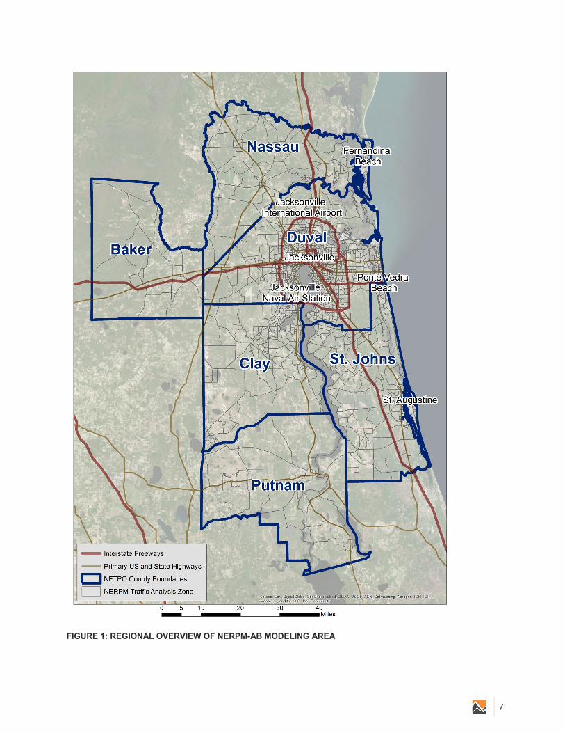
7
FIGURE 1: REGIONAL OVERVIEW OF NERPM-AB MODELING AREA

V 1.0 Northeast Regional Planning Model: Activity Based Calibration and Model Validation Report
8 February 12, 2015
The SHRP 2 C10A dynamic network modeling approach, however, proved to be challenging and was not ready for production use at the end of the C10 project. For this reason and for the sake of consistency with the Florida Standard Urban Transportation Model Structure (FSUTMS), the 2010 version of the model was integrated with the more conventional network assignment methods and auxiliary models used by North Florida TPO and other regional planning agencies in the United States. Work to calibrate and validate the new modeling system began prior to the LRTP process, with final validation completed during its early stages.
1.2 | SCOPE OF WORK COMPLETED
NERPM-AB is composed of many different model components. The work required to complete model system included developing:
a synthetic population of residents living in households and group quarters; employment by industry group; a parcel-based land use database; parameters for activity-based residential demand models, covering travel within the region; calibration target values for activity-based model components, using NHTS survey data, U.S. Census
ACS household travel characteristics, and CTPP; updated trip tables representing non-resident travel and resident travel with external trip ends
(external-external, external-internal, internal-external); updated truck-trip generation and distribution models from the Florida statewide model and from
Jacksonville Port facilities; updated special generators for Jacksonville International Airport and for the tourism district of St.
Augustine; updated highway network files, requiring recoding of some link attributes, removal of intersection
turning penalties, and speed-capacity tables; updated transit route files; new highway assignment procedures and skimming methods for four time periods (AM Peak, Midday,
PM Peak, and Evening off-peak), as well as summaries for full-day analysis; updated traffic count data; and new speed-feedback procedures and closure criteria.
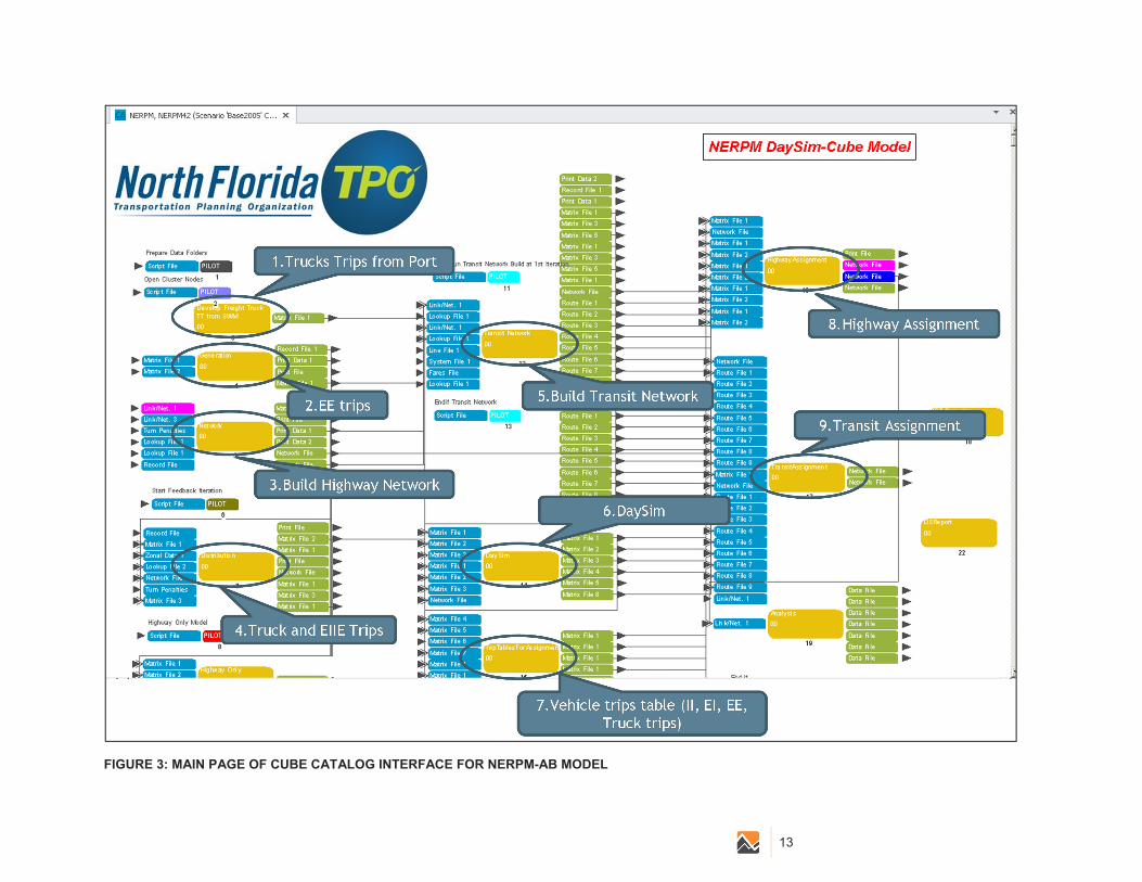
The model components listed above were integrated into a single package within the Citilabs® Cube travel demand modeling system, using the Cube Catalog graphic user interface (GUI) organizational format previously developed for NERPM trip-based models. A full description of each of these components is to be included in a NERPM-AB User’s Guide. Once all of the above components were in place, the work of calibrating and validating the NERPM-AB model began.
1.3 | APPROACH TO CALIBRATION
At the heart of the NERPM-AB system is DaySim, an integrated suite of complex models that, together, simulate the daily travel patterns of individuals residing in the North Florida TPO modeling region. This new, six-county 2010 regional activity-based model was calibrated to match regional target values, most of which were derived from the 2008–2009 NHTS add-on for the State of Florida. The original plan under SHRP 2 C10A was to estimate a new set of DaySim parameters, based on the Sacramento specification, but using the NHTS data using a pooled sample of Jacksonville and Tampa Bay regional households. The idea behind a

9
pooled sample was to provide a sufficient number of observations for model estimation; however, the SHRP 2 C10A study team deemed this approach infeasible after extensive attempts at estimating new parameters.1
The 2008–2009 NHTS Florida add-on survey captured responses from 1,335 households in the Jacksonville region and 2,517 households in the Tampa Bay region, and did not include separate records of household members younger than five years of age. Moreover, many of the household diary days in the Jacksonville and Tampa Bay samples were weekends, which could not be used for estimating models of daily patterns, tours or trips due to the weekday focus of the model specification, reducing the useable sample size to less than 1,000 households for the Jacksonville region. Further, the SHRP 2 C10A study team’s analysis of model estimation results revealed that prevailing travel patterns in the Jacksonville regional sample were actually more similar to those of Sacramento than to the Tampa regional sample, most likely due to the much higher proportion of retiree households in the Tampa region.
For these reasons, it was determined that a more behaviorally sound model would result from transferring the original set of Sacramento parameters and calibrating to target values specific to the six-county Jacksonville region, which was done. Described in more detail below, the NHTS sample for the Jacksonville region provided a sufficient number of observations from which to calibrate model parameters for the vast majority of DaySim model components; however, it was desirable to supplement the NHTS target values with other sources of validation data for some model components.
1 Gliebe J, Bradley M, Ferdous N, Outwater M, Lin H and Chen J. SHRP 2 C10A. Transfer of Activity-Based Model Parameters from Sacramento to Jacksonville and Tampa, Florida: Preliminary Draft. Final Report. Transportation Research Board. March 2014. (http://www.trb.org/Main/Blurbs/170748.aspx , last accessed June 29, 2014.)

V 1.0 Northeast Regional Planning Model: Activity Based Calibration and Model Validation Report
10 February 12, 2015
2.0 MODEL SYSTEM COMPONENTS
The NERPM-AB model is designed for regional-scale policy analyses and planning applications. This report provides a brief, non-mathematical description of each of the core activity-based model components of the NERPM-AB model to provide readers with an understanding of each model component and its purpose.
Figure 2, below, is a high-level representation of the major model system components and the general programmatic flow between them. Four preliminary data preparation steps are run separately from the main travel model. The main portion of the modeling runs within the Cube Voyager system. Figure 2 shows these steps in order of their functional relationships, which may different slightly from the actual order in which they are executed in the Cube system.
FIGURE 2: NERPM-AB V1.0 MODEL SYSTEM FUNCTIONAL RELATIONSHIPS

11
2.1 | DATA PREPARATION STEPS
NERPM-AB v.1.0 maintains 2,494 internal TAZs, which are the basis for modeling vehicular trip ends and for maintaining aggregate totals of housing units, household types, employment, school enrollment and hotels and motels.
An additional 28 external TAZs serve as gateways for external trip ends, but do not have any land use data associated with them.
There are 492,684 parcels in the 2010 base-year scenario of NERPM-AB v.1.0, each of which contains land use data on a particular property, such as development codes, number of housing units, and square-feet of leasable commercial floor area. Parcels nest within the internal TAZs and are used as the spatial units to which households, employment and school enrollment are allocated. Their role in the DaySim modeling system is for calculating short-distance trip lengths, transit walk access, and land use accessibility/attractiveness variables.
A synthetic population is generated using a program called PopGen (See Section 5.0 for details), which creates a database of households and persons within households representing the real-world population of the region. The distribution of households is controlled by TAZ, then allocated to land-use parcels within each TAZ where housing units are indicated.
Employment and school and college/university enrollment data are allocated to parcels to match known locations of existing land uses and are allocated to parcels with appropriate zoning and capacity for forecast-year development.
The all-streets network is a detailed GIS network, developed from NAVTEQ data. Land-use parcel and transit-stop locations are associated with the nearest node in the all-streets network to provide estimates of short (less than 3 miles) trip distances and walking distance to transit stops.
The enhanced all-streets network with transit stop locations is then combined with land-use parcel file, which also includes employment data by various industry types, to create a variety of urban form variables, called buffer variables, that measure the accessibility of parcels to households and employment. DaySim uses these variables in different parts of the activity-based demand model, most notably in the models that generate tours and intermediate stops on tours.
2.2 | PRIMARY MODELING STEPS
As show in Figure 2, the first primary modeling steps are the generation of skims and the distribution of some auxiliary demand. NERPM-AB runs a feedback loop that returns highway assignment skims for use in all demand-generating steps.
Within this feedback loop, are DaySim, a regional truck and freight model, and an external trips model. In addition, the model includes two special generators—Jacksonville International Airport and the historic City of Saint Augustine. DaySim accounts for all travel by residents of the North Florida TPO region for their travel within the region.
The truck and freight model includes all trips made for transportation of goods and services and includes a Jacksonville area Port Model. The external trips model includes both internal-external (trips made by region residents to points outside the region), external-internal (trips made by residents from outside the region to points within the region), and through trips. All of the mode components use the TAZ system and are adapted from previous NERPM trip-based models. Trips from all the sub-models are aggregated and factored to create trip tables, which are then assigned to the highway and transit networks.

V 1.0 Northeast Regional Planning Model: Activity Based Calibration and Model Validation Report
12 February 12, 2015
The model system runs network assignment for AM Peak, Midday Off-Peak, PM Peak and Evening Off-Peak periods. (See Section 4.0 for details.)
The feedback loop currently is configured to run four (4) global iterations to ensure good convergence for each network assignment period. Once convergence has been achieved and final highway assignment have been created, the model system exits the feedback loop, runs Peak and Off-Peak transit assignments, and produces a set of diagnostic reports and DaySim tabular output files.
A sample of the Cube catalog user interface is shown in Figure 3. DaySim is implemented as a standalone executable program within the Cube Catalog. All non-DaySim components are written in Cube scripts, such as trip aggregation methods, auxiliary demand models, highway and transit network-assignment models and skimming processes. These scripts were adapted from NERPM v4.2. Additional scripts for summarizing DaySim model outputs were written in the “R” open-source statistical programming language.2
2 R Development Core Team (2011). R: A language and environment for statistical computing. R Foundation for Statistical Computing, Vienna, Austria. ISBN 3-900051-07-0, URL http://www.R-project.org/.
13
FIGURE 3: MAIN PAGE OF CUBE CATALOG INTERFACE FOR NERPM-AB MODEL

V 1.0 Northeast Regional Planning Model: Activity Based Calibration and Model Validation Report
14 February 12, 2015
3.0 OVERVIEW OF DAYSIM MODEL SYSTEM
The DaySim model developed for North Florida TPO represents travel demand patterns for a “typical” weekday. The underlying assumption is that schools are in session and that it is not a holiday. Figure 4 depicts the structure of the DaySim model components used in the NERPM-AB model. It includes models at five different levels:
Long-term choices—the typical work and school locations and auto ownership. Person-day-level choices—the number of tours to make for each activity purpose, and the inclusion
of additional activities to be performed on those tours. Tour-level choices—the primary destination, main mode, destination, and arrival and departure
times for each tour. Half-tour-level choices—the number and purpose of any intermediate stops between the home
anchor point of the tour and the primary destination of the tour. Trip-level choices—the location of intermediate stops and the mode and departure time of each
trip.
In Figure 4, the white and gray arrows represent the flow of model application, from one module to the next. The colored arrows represent feedback paths in which the expected utility from downstream choices (log sums) influence the choices made upstream. Each choice is conditioned by the choices simulated “above” it, but is also influenced by “log sums” (expected utilities) of the possible choices “below” it (colored arrows). Log-sums, so named because they are calculated from the natural log of the sum of the denominator of a discrete choice model, represent the composite utility of a set of choices. In this way, the log sums calculated from a “downstream” choice model can be used as accessibility variables (travel times and costs) to influence the “upstream” choices that come before it. For example, log sums calculated from mode choice models are often used as variables in upstream destination choice models and, in this way, represent the attractiveness of available mode options for each destination being considered, without knowing which mode will be chosen. Log sums recur throughout the DaySim model system to ensure both upward and downward consistency.

15
FIGURE 4: STRUCTURE OF DAYSIM

V 1.0 Northeast Regional Planning Model: Activity Based Calibration and Model Validation Report
16 February 12, 2015
4.0 DATA DEVELOPMENT AND INTEGRATION
Integration of the activity-based modeling components with the supply-side and auxiliary demand model components involved several data preparation steps. An abbreviated summary of the major tasks follows.
4.1 | PARCEL BASED LAND USE DATA
The Sacramento version of DaySim was notable for, among other things, the first activity-based modeling system in the United States to use parcel-level land-use inputs. The primary benefit of this approach is greater spatial precision in terms of activity locations, pedestrian and bicycle travel time estimation, and walk access to transit. Although it would have been possible to transfer the Sacramento model to a system that used more aggregate spatial units, it was necessary to develop DaySim accessibility variables at the parcel level for the Jacksonville region.
North Florida TPO and the consultant team developed GIS-based point and polygon layers of land use for each of the counties in the model area. This process was the most time-consuming of the integration steps, primarily because staff for both agencies viewed this as the development of an operational regional modeling system and wanted to perform thorough reviews and quality assurance checking. This process involved reconciling logical inconsistencies between tax assessors’ records for housing units and commercial square footage, Census records for households, and establishment-level employment data purchased from a commercial vendor, InfoGroup. Although the Florida Department of Revenue has a set of consistent definitions for coding tax-assessor database entries, adherence to these standards was inconsistent between counties. In addition, there were, in some cases, multiple versions of the GIS layers, which varied in the extent to which polygon slivers had been cleaned and recoded based on previous work efforts.
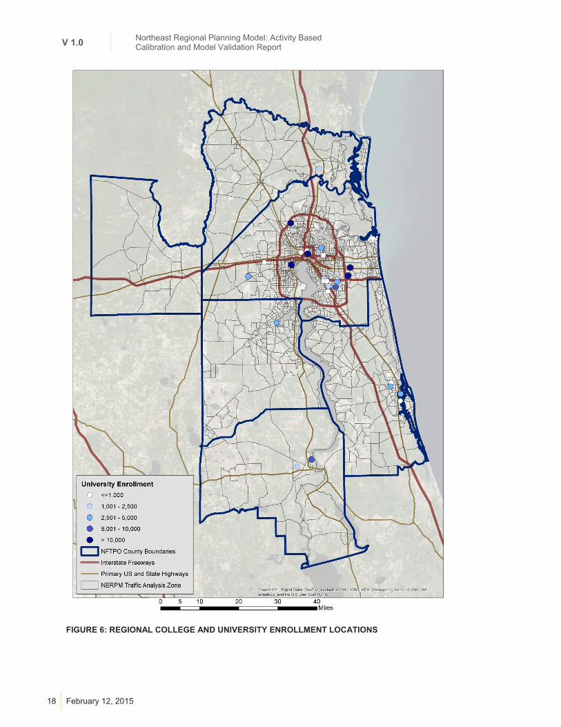
For the DaySim model, the critical parcel attribute fields were the number of single-, multi-family, and “other” housing units; number of paid parking spaces; and K-12 school enrollment and post-secondary (college/university) enrollment. A summary of these attribute quantities is shown below in Table 1 and in Figure 5 and Figure 6 for K-12 and college/university, respectively. Parking and enrollment data were added to the base parcel layer by agency staff and local consultants. As described below, households and employment were also assigned to parcels; however, the processes were more complicated due to the need to maintain regional control totals.
TABLE 1: SUMMARY OF CRITICAL PARCEL ATTRIBUTES
Parcel Attribute Quantities
Number of single-family housing units
405,574
Number of multi-family housing units
165,017
Number of other type housing units (retirement home, mobile-house, etc.)
65,155
Number of paid parking spaces
3,124
K-12 school enrollment
249,010
Post-secondary (college/university) enrollment
121,885

17
FIGURE 5: REGIONAL K-12 STUDENT ENROLLMENT LOCATIONS
V 1.0 Northeast Regional Planning Model: Activity Based Calibration and Model Validation Report
18 February 12, 2015
FIGURE 6: REGIONAL COLLEGE AND UNIVERSITY ENROLLMENT LOCATIONS

19
4.2 | REGIONAL HOUSEHOLDS AND EMPLOYMENT
To support the development of synthetic populations and to control the spatial distribution of regional employment, North Florida TPO developed regional control totals for households and employment.
HOUSEHOLDS
Regional household control totals were specified for multiple attributes and attribute levels, using the 2010 Census at the Block Group level. These control totals were then mapped to NERPM’s TAZ system for consistency with past practices and future forecasts. Control totals were developed for three separate population groups: permanent residents living in households, seasonal resident households, and group quarters residents. Table 2, below, shows the number of households by type in each region. North Florida TPO reviewed these data at the TAZ level and provided recommendations for minor adjustments, primarily to the locations of group quarters and seasonal populations, based on local knowledge. The consultant team used these regional control totals, along with household sample data from ACS PUMS, to produce synthetic 2010 populations for each region, using the open-source program, PopGen 1.1, simultaneously controlling both household- and person-attribute levels.
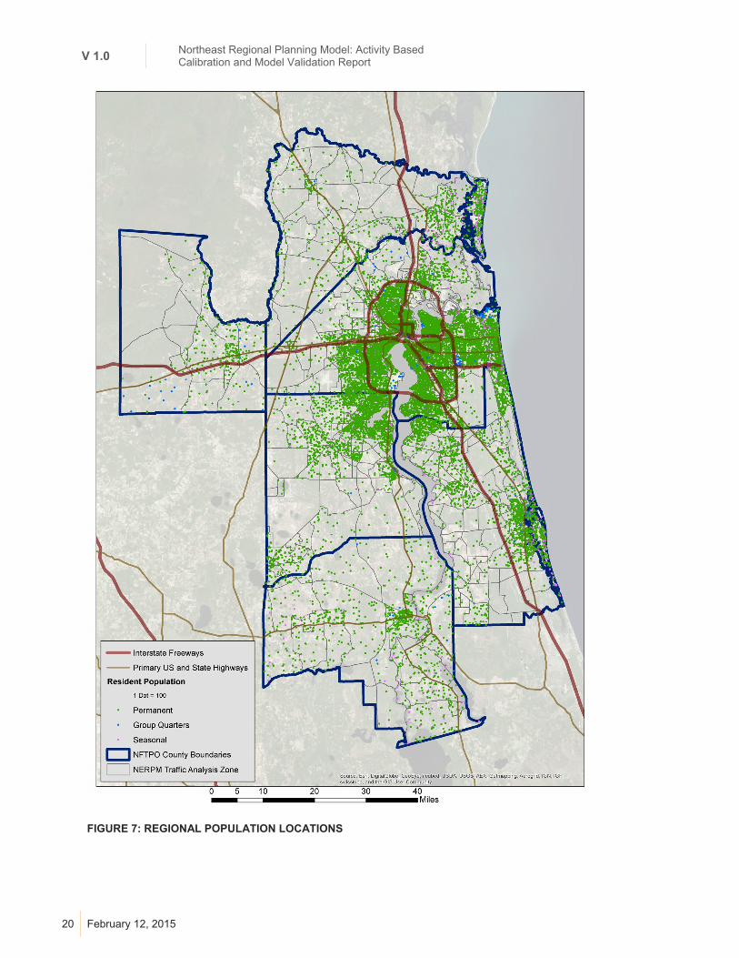
Once a set of synthetic households and persons were created at the TAZ level, the consultant team applied a utility program to allocate them to the parcel level, using the locations of housing units found in the parcel data. As shown below in Figure 7, permanent residents, the green dots on the map, are concentrated primarily within the urban core of the Jacksonville metro area and along the coastal communities, but smaller cities and towns show up in each of the outer counties. Group quarters residents, represented by blue dots, are concentrated in a handful of clusters within Duval County, with additional group quarters residents sprinkled throughout the other counties. Seasonal residents, represented by pink dots, are concentrated in the resort areas along the coast in St. John’s, Duval and Nassau Counties.
TABLE 2: NUMBER OF HOUSEHOLDS BY TYPE
Type Number
Permanent residents household 553,265
Group quarters 16,854
Seasonal residents household 28,328
V 1.0 Northeast Regional Planning Model: Activity Based Calibration and Model Validation Report
20 February 12, 2015
FIGURE 7: REGIONAL POPULATION LOCATIONS

21
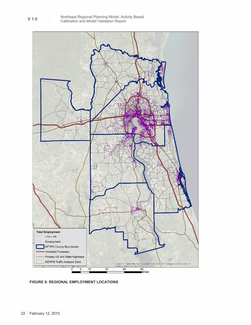
EMPLOYMENT
Due to differences in the ways that employment data are collected and classified by various sources, multiple sources of employment were used. North Florida TPO acquired 2010 establishment-level data from the commercial vendor, InfoGroup, and these data were then geocoded to individual parcel locations. North Florida TPO used regional employment control totals provided by the Florida Bureau of Economic and Business Research (BEBR). These corresponded roughly with the region-wide totals for InfoGroup, but varied by industry and county. Summaries of employment by industry from each source and the final employment numbers may be found in Table 3, below. The location of total employment across the region is shown below in Figure 8. This map clearly shows that the bulk of the region’s employment is concentrated in Duval County, with smaller employment clusters in surrounding counties. The concentration is employment along freeways and other major highway corridors is also quite evident in Figure 8.
TABLE 3: EMPLOYMENT DATA BY INDUSTRY TYPE AND SOURCE
Industry Title
Florida Bureau of Economic
and Business Research (BEBR)
2010 Quarterly Census of
Employment and Wages
(QCEW)
INFO Group
Final employment data used in
the model
Agriculture, Forestry, Fishing and Hunting 1,771 1,901 1,646 2,080
Mining 97 124 421 420
Utilities 788 3,427 1,935 1,937
Construction 28,199 27,815 54,486 51,998
Manufacturing 28,839 28,772 47,356 47,509
Wholesale Trade 23,346 23,168 27,729 26,443
Retail Trade 71,137 71,707 92,234 90,336
Transportation and Warehousing 24,919 30,172 27,065 27,083
Information 10,013 9,996 16,892 16,832
Finance and Insurance 45,324 45,172 45,485 46,078
Real Estate Rental and Leasing 8,797 8,618 18,455 16,952
Professional, Scientific, and Technical Services
32,531 33,256 37,163 35,687
Management of Companies and Enterprises 5,705 5,701 488 5,746
Administrative and Support and Waste Management and Remediation Services
41,940 42,088 25,722 40,938
Educational Services 8,854 40,922 44,031 43,066
Health Care and Social Assistance 75,649 77,662 77,199 76,661
Arts, Entertainment, and Recreation 8,770 9,549 8,448 9,299
Accommodation and Food Services 56,301 56,391 63,433 61,204
Other Services (except Public Administration)
17,274 16,862 34,002 31,374
Public Administration 0 33,967 69,396 60,337
Total 490,254 567,270 693,586 691,980
V 1.0 Northeast Regional Planning Model: Activity Based Calibration and Model Validation Report
22 February 12, 2015
FIGURE 8: REGIONAL EMPLOYMENT LOCATIONS

23
The consultant team developed a program to synthesize missing employment and randomly remove disaggregate employment records in places where county control totals for a particular industry segment were exceeded. Missing jobs by industry group were added to parcels with appropriate land-use designations, favoring locations where such jobs already existed, so that taken together they matched county-level control totals. Agency staff performed extensive reviews of these synthesized disaggregate job records and specified manual re-allocations, as necessary.
4.3 | NETWORK MODELS
Prior versions of the NERPM model had only a peak period and daily highway-network assignment periods. Consistency with the AB model design of DaySim necessitated the development of separate highway network assignment and skimming processes for four time-periods of the day:
AM Peak (6:00-8:59 a.m.); Midday Off Peak (9:00 a.m.-3:59 p.m.); PM Peak (4:00-6:59 p.m.); and Evening Off Peak (7:00 p.m.-5:59 a.m.).
These four time-period-based assignments are run individually, producing a loaded network for each period. At the end of the process, a new script is then run to combine all four time periods into a single Daily assignment output, representing a 24-hour travel period. Transit assignments use methods adapted from the NERPM v4.2 model. Two transit assignments are run: a Peak Period assignment based on AM Peak level of service conditions, and an Off-Peak assignment, based on Midday Off-peak based level of service conditions.
In addition, the consultant team modified the speed-feedback loop system, using skim-averaging methods, which improved convergence rates after integration with DaySim. The speed-feedback loop was modified to account for multiple (four) network-assignment time periods.
4.4 | MARKET SEGMENTATION AND AUXILIARY DEMAND
The NERPM-AB modeling system covers regional land-based travel, segmented by four primary markets:
Resident travel internal to the modeling region; Non-resident/visitor travel internal to the modeling region; Resident and non-resident/visitor travel involving trips passing through the region, but with at least
one end outside the region; and Freight and other commercial vehicle travel internal to the modeling region as well as truck travel with
at least one end outside the region;
The DaySim AB model covers all household resident travel within the region for the following market segments:
Permanent residents living in households; Permanent residents living in group quarters; and Seasonal residents living part of the year in the region, who are permanent residents of a different
region.
DaySim does not cover visitors to the region, such as tourists, business travelers and non-residents visiting family and friends. Nor does DaySim cover travel by persons who live external to the modeling area, but who
V 1.0 Northeast Regional Planning Model: Activity Based Calibration and Model Validation Report
24 February 12, 2015
may commute in and out of the region for work or school, or who come to the region for shopping, recreation or other personal business.
NERPM v4.2 used a list of special generators to supplement the usual productions and attractions; however, this included many sites that are considered to be covered by DaySim in NERPM-AB. Common special generators, such as hospitals, shopping malls and military installations are covered by the resident travel models listed above. Two special generators were retained in NERPM-AB: (1) Jacksonville International Airport (15,000 daily trip ends, derived from airline enplanements); and (2) St. Augustine’s historic center (2,288 daily trip ends, derived from hotel and motel rooms). Both of these special generators represent concentrations of intense visitor traffic, which are not covered by DaySim.
External trip ends are handled by processes retained from NERPM v4.2 for creating external-internal (EI), internal-external (IE), and external-external (EE) trip tables. IE/EI trips are intriguing because, in theory, they overlap with activities and travel generated by households through DaySim. For example, persons who live within a region, but who work or attend school outside of the region, have IE tour and trip patterns. In DaySim, a fixed portion of workers and students are assumed to have usual work or school locations outside of the study area. These IE work and school commutes are predicted, and the entire day pattern for these individuals is not used in subsequent model steps to create trip tables because it would duplicate the IE flows that already exist in the model. The portion of workers in each TAZ that work outside the region is derived from ACS journey-to-work data. Intuitively, persons who live near the edges of a study region are more likely to work outside of it than those who live closer to the center.
DaySim assumes that a portion of the jobs within the region will be filled by workers who live outside the region. To accommodate this market, EI work trips are fixed for workplace destinations, thereby reducing the availability of those jobs for workers living within the region. The usual workplace location choice is affected by DaySim’s shadow-pricing mechanism, which compares the total employment within each zone to the number of workplace locations predicted for each zone and adjusts the attractiveness of that zone through a series of iterations to balance job supply with worker demand. Trial-and-error revealed that a ten-iteration approach to shadow pricing for employment was sufficient to create a converged set of shadow-pricing factors.
4.5 | TRUCK AND PORT MODELS
NERPM-AB includes three separate types of data models that, together, represent regional truck traffic. NERPM-AB borrowed the methods, coded in Cube script, directly from NERPM v4.2. As described below, the consultants updated the input data for these three models.
TRIP-BASED COMMERCIAL VEHICLE MODEL (CVM)
NERPM v4.2 represents intra-regional short-haul goods and commercial service trips using trip generation and distribution rates adapted from the Quick Response Freight Model (QRFM), which forecasts truck trips based on TAZ-level employment and households. For NERPM-AB, the consultants did not modify this procedure in any way, retaining all trip-generation rates and trip-distribution friction factors developed for NERPM v4.2. The consultants did, however, update the socioeconomic data in the ZDATA file to reflect 2010 and 2040 employment and households—key inputs to the CVM.

25
STATEWIDE FREIGHT MODEL (SFM) INPUTS
Inter-regional truck movements are static inputs from the Florida Statewide Freight Model (SFM). NERPM v4.2 derives SFM trip tables from a sub-area extraction of the statewide model network. For NERPM-AB, the consultant team began with the 2005 and 2030 statewide truck trip tables and used simple linear interpolation to grow 2010 and 2040 trip tables on a cell-by-cell basis.
Upon reviewing these tables, the consultant team decided to revise the 2010 truck trip tables to use 2005 numbers to reflect the fact that the period between 2006 and 2010 was recessionary. The U.S. Bureau of Economic Analysis (BEA) showed zero growth in Florida’s gross domestic product (GDP) from 2006 to 2010. Moreover, AADT counts at the I-10 and I-95 external stations showed slight decreases in total traffic between 2005 and 2010. The consultants did not revise the 2040 trip table, assuming that the longer-term growth trend would continue on an upward trajectory, following to the 2005-2030 rate of change forecast by the SFM.
JAXPORT MODEL
Northeast Florida is a busy intermodal freight hub, with seaports at Jacksonville and Fernandina, marine terminals along the St. John’s River, and large freight railroad yards for CSX, Florida East Coast (FEC) and Norfolk-Southern (NS). The JAXPORT model represents intermodal movements between marine terminals, railroads and trucks at several important intermodal facilities. Table 4 below lists nine intermodal facilities, their TAZ locations, and fields representing model parameters, with values for the 2010 base year.
For the sake of completeness, the table includes the JAXPORT Cruise Facility; however, this terminal currently serves only passenger ships and therefore does not generate freight container trips.
Fields definitions are as follows.
TYPE – Terminal Type
1 = Port (marine) terminal
2 = Intermodal rail yard
TRIPENDS – Daily truck trip ends expected to enter and exit the terminal, measured in twenty-foot equivalent units (TEU), an industry standard, approximating cargo containers.
− Note that in Table 4 there are positive values only for the Type-1 port terminals. This is because the model assumes that the SFM determines the trip ends for the Type-2 rail yard terminals.
HWY_FRAC – Fraction of TEUs that enter and leave Type-1 port facilities by highway as a truck trip.
− A value less than 1.0 would indicate that some portion of TEUs are transferred directly between ship and rail and do not use the highway network; however, all of the entries in Table 4 are 1.0, as there was no information to assume otherwise. Type-2 intermodal rail yards do not use HWY_FRAC.
IM_FRAC – Proportion of TEUs allocated to Type-2 intermodal rail yards.

V 1.0 Northeast Regional Planning Model: Activity Based Calibration and Model Validation Report
26 February 12, 2015
− For Type-1 (port terminals), IM_FRAC represents the proportion of trip ends entering or leaving the port that come from or go to Type-2 intermodal rail yards. The port truck model allocates the remainder to other destinations within the region or to external stations.
− For Type-2 (intermodal rail yards), IM_FRAC represents the proportion of truck trips in the SFM tables that travel to and from external stations to each of the Type-2 facilities. The sum of the IM_FRAC for all Type-2 facilities must equal 1.0. For example, the entries in Table 4 imply that 50 percent of the EI/IE truck trips from the SFM will have one trip end at the CSX intermodal rail yard, while the remainder are split evenly between FEC and NS rail yards.
TABLE 4: 2010 JAXPORT INPUT FILE
INDEX NAME ZONE TRIPENDS HWY_FRAC IM_FRAC TYPE
1 CSX Intermodal 187 0 0.00 0.50 2
2 FEC Intermodal 268 0 0.00 0.25 2
3 NS Intermodal 333 0 0.00 0.25 2
4 JAXPORT Cruise 351 0 1.00 0.00 1
5 Fernandina 367 400 1.00 0.10 1
6 Blount Island 415 2,471 1.00 0.10 1
7 Dames Point 416 991 1.00 0.10 1
8 Talleyrand1 439 1,117 1.00 0.14 1
9 Talleyrand2 440 312 1.00 0.14 1
Total 5,291
TABLE 5: 2040 JAXPORT INPUT FILE
INDEX NAME ZONE TRIPENDS HWY_FRAC IM_FRAC TYPE
1 CSX Intermodal 187 0 0.00 0.54 2
2 FEC Intermodal 268 0 0.00 0.23 2
3 NS Intermodal 333 0 0.00 0.22 2
4 JAXPORT Cruise 351 0 1.00 0.00 1
5 Fernandina 367 1,220 1.00 0.10 1
6 Blount Island 415 6,341 1.00 0.12 1
7 ICTF 415 0 0.00 0.01 2
8 Dames Pt + 2nd term. 416 6,106 1.00 0.10 1
9 Talley Rand 1 439 1,301 1.00 0.00 1
10 Talley Rand 2 440 367 1.00 0.00 1
Total 15,335
Table 5 is the 2040 JAXPORT input file. This reflects the addition of two new facilities expected to be operating in 2040—a second terminal at Dames Point and the Intermodal Container Transfer Facility (ICTF)

27
at Blount Island. IM_FRAC values for 2040 reflect a future split among the Type-2 rail-yard facilities, based on assumed 2040 capacities, inclusive of these two new facilities. Total truck trip ends at the Type-1 port facilities reflect historical growth trends in port container traffic that are expected to result in a tripling of trip ends from 2010 to 2040. Allocation of trip ends between the Type-1 facilities is proportional to anticipated future capacities at each location.
4.6 | URBAN FORM AND ACCESSIBILITY VARIABLES
DaySim uses parcels as the main spatial unit; therefore, it is important to have measures of what lies on any particular parcel as well as what lies in the area immediately surrounding each parcel. These measures are created by defining a “buffer” area around each parcel and counting what lies inside the buffer. These variables can then be used in DaySim in a way similar to how zonal land-use and density variables are used in TAZ-based models, with the advantage that the buffer is defined in exactly the same way for each parcel. The buffer variables that DaySim uses include:
The number of households in the buffer; Employment (number of jobs) in the buffer in various employment sectors; Enrollment in schools in the buffer, segmented by grade schools and colleges; The number of spaces and average price of paid, off-street parking in the buffer; The number of transit stops within the buffer (segmented by mode, if relevant); The number of street intersections in the buffer, segmented by 1-node (dead-end or cul-de-sac), 3-
node (T-junction), and 4+node intersections; and The area within the buffer that is public, open space (parks, etc.).
A custom set of buffering programs create the buffering variables for each parcel. These programs combine the GIS parcel layer, complete with attributes listed above, along with the all-streets network, to calculate the variables. The buffering calculations require the input of an “all streets” network to count all local streets and intersections, not just the higher-level facilities used in the regional highway network model. North Florida TPO acquired a NAVTEQ network for this purpose.

V 1.0 Northeast Regional Planning Model: Activity Based Calibration and Model Validation Report
28 February 12, 2015
5.0 POPULATION SYNTHESIS
NERPM-AB is a microsimulation model that forecasts travel based on a disaggregate representation of individual travelers. It represents individual travelers and their households in the simulation through a synthetic population. The consultant team developed the synthetic population using the open-source program PopGen v.1.1, developed by Arizona State University’s Fulton School of Engineering.3 Attributes of the synthetic population were specified to provide the household and person variable inputs to DaySim. The consultant team calibrated the distributions of attributes of the synthetic households and persons to match those of the real-life population for the region, based on the 2010 U.S. Census and the American Community Survey (ACS) 2006-2010.
Three primary market segments comprise the synthetic population for the six-county modeling region:
Permanent residents living in households
− 553,265 households − 1,391,004 persons
Seasonal residents living in households
− 16,854 households − 34,675 persons
Permanent residents living in non-institutionalized group quarters (GQ)
− 28,328 persons
Figure 7, above, shows the locations of concentrations of each of these populations segments throughout the region. Permanent residents living in household comprise 96 percent of the synthetic population and 94 percent of synthetic households. For modeling purposes, GQ residents are treated as one-person households.
They represent households of persons who live part of the year in Northeast Florida, but who are permanent residents in another region and therefore do not show up in the Census totals for the six-county North Florida TPO modeling area. North Florida TPO identified the locations of households with seasonal residents in the coastal communities of St. Johns, Duval and Nassau Counties. Their inclusion allows NERPM-AB to represent peak seasonal demand conditions; however, it is possible to exclude the seasonal population to represent lower seasonal demand.
5.1 | CALIBRATING THE SYNTHETIC POPULATION
Creation of a synthetic population begins by supplying PopGen with marginal distributions for the household and person attributes of interest as well as a sample data set that represents how these same attributes are correlated within the population. As a simple example, two commonly used attributes are the distribution of households by their size (number of person: 1, 2, 3, 4, 5+) and the distribution of households by household income group, as typically found in the Census. For each attribute, the total number of households should equal the total for the region. A sample data set would represent actual households records, as typically found in the ACS Public Use Microdata Sample (PUMS). If household size and income were the only two attributes
3 http://urbanmodel.asu.edu/popgen.html
29
of interest, PopGen would generate synthetic household records such that the marginal control totals were met for both households by size bin and households by income bin, while using the correlation between size and income bins found in the sample data. The method for doing this involves iterative proportional fitting (IPF) in which the sample data is the seed matrix and the marginal control totals are target values. This method is similar to the “fratar” methods used in balancing trip tables.
The method used to develop the synthetic population for NERPM-AB is a bit more complicated, however, because it involves balancing to both household- and person-level attributes and control totals across more than two dimensions. In addition, the sample data also contains both household records and person records. When PopGen is run with both household- and person-level controls, it will attempt to satisfy all of the marginal control totals at both levels. With a larger set of attributes and both household- and person-level controls, it is typically not possible to match all of the marginal control totals. This is because the sample records may not include enough of the right combinations of household attributes, which is often the case with rare combination, such as households with more than seven persons. In addition, it is difficult to satisfy both household- and person-level control totals simultaneously, particularly when it comes to ages of householder and presence of children, as specified at the household level, and the number of persons by age group as specified at the person level. The user is able to specify whether PopGen will place more weight on matching the household-level control totals or more weight on the person-level control totals. Historically, transportation planning has focused on household units; therefore, the consultants prioritized fit to the household-level marginal distributions.
In terms of process, the consultants developed the marginal control totals using NERPM TAZs as the fundamental spatial unit for all-three market segments. The consultant team allocated marginal distributions from their original sources, Census blocks and ACS block groups for the permanent resident population to TAZs for both household and GQ residents. North Florida TPO reviewed and approved the final allocations after consultation with local planners.
For seasonal residents, North Florida TPO identified TAZs with known concentrations of resort condominium housing units. For each TAZ, North Florida TPO derived the percentage split between permanent and seasonal housing units through land use database review and communication with planners serving these communities. Marginal control totals for seasonal residents utilized a distribution of demographic attributes for seasonal households identified in the NHTS survey Florida add-on, using the sample for the entire state.
5.2 | PERMANENT RESIDENTS LIVING IN HOUSEHOLDS
Table 6 below lists the attributes of households used to define the permanent resident portion of the synthetic population. The table shows six attributes, stratified by bins. The sixth attribute in the table, the persons-by-workers joint variable represents combinations of household size and number of workers, which has been found to be a good predictor of the number of workers in the household.
The marginal distributions of households by age of householder, household size, dwelling unit type, and presence of children were derived from 2010 Census data at the block level. The marginal distributions of households by income and the joint distribution of households by size and number of workers were derived from ACS at the block-group level.

V 1.0 Northeast Regional Planning Model: Activity Based Calibration and Model Validation Report
30 February 12, 2015
The attributes of persons used to define the resident portion of the synthetic population are listed below in Table 7. Both gender and age marginal control totals were derived from the Census at the block level.
TABLE 6: RESIDENT HOUSEHOLD-LEVEL MARGINAL CONTROL TOTALS VS. SYNTHESIZED HOUSEHOLDS
Marginal Distribution Categories Control
Total Households
Synthesized Totals
% Difference
Householder age 1 Householder 15 to 24 years 27,330 27,023 -1.1% 2 Householder 25 to 54 years 308,550 309,302 0.2% 3 Householder 55 to 64 years 102,886 102,758 -0.1% 4 Householder 65 to 74 years 63,504 63,413 -0.1% 5 Householder 75 years-plus 50,995 50,769 -0.4% Total 553,265 553,265 0.0%
Household size 1 1-person HH 143,842 144,264 0.3% 2 2-person HH 189,340 189,794 0.2% 3 3-person HH 95,094 94,836 -0.3% 4 4-person HH 73,206 72,973 -0.3% 5 5-person HH 32,514 32,299 -0.7% 6 6-person HH 12,219 12,099 -1.0% 7 7 or more-person HH 7,050 7,000 -0.7% Total 553,265 553,265 0.0%
Household unit type 1 SFD 403,811 404,041 0.1% 2 MFD 149,454 149,224 -0.2% Total 553,265 553,265 0.0%
Presence of children 1 Yes 184,806 184,406 -0.2% 2 No 368,459 368,859 0.1% Total 553,265 553,265 0.0%
Family annual income 1 Less than $20,000 93,121 93,112 0.0% 2 $20,000 to $39,999 117,581 117,768 0.2% 3 $40,000 to $59,999 102,526 102,592 0.1% 4 $60,000 to $99,999 135,166 135,214 0.0% 5 $100,000 or more 104,871 104,579 -0.3% Total 553,265 553,265 0.0%
Persons by workers joint variable 1 1-persons, no worker 64,380 64,616 0.4% 2 1-persons, 1 worker 79,462 79,648 0.2% 3 2-persons, no workers 51,366 51,498 0.3% 4 2-persons, 1 worker 66,417 66,384 0.0% 5 2-persons, 2 workers 71,557 71,912 0.5% 6 3-persons, no worker 8,501 8,395 -1.2% 7 3-persons, 1 worker 35,668 35,544 -0.3% 8 3-persons, 2 workers 37,444 37,447 0.0% 9 3-persons, 3 workers 13,481 13,450 -0.2%
10 4 or more-persons, no workers 7,795 7,806 0.1% 11 4 or more-persons, 1 worker 43,047 42,902 -0.3% 12 4 or more-persons, 2 workers 51,501 51,403 -0.2% 13 4 or more-persons, 3 or more workers 22,646 22,260 -1.7% Total 553,265 553,265 0.0%
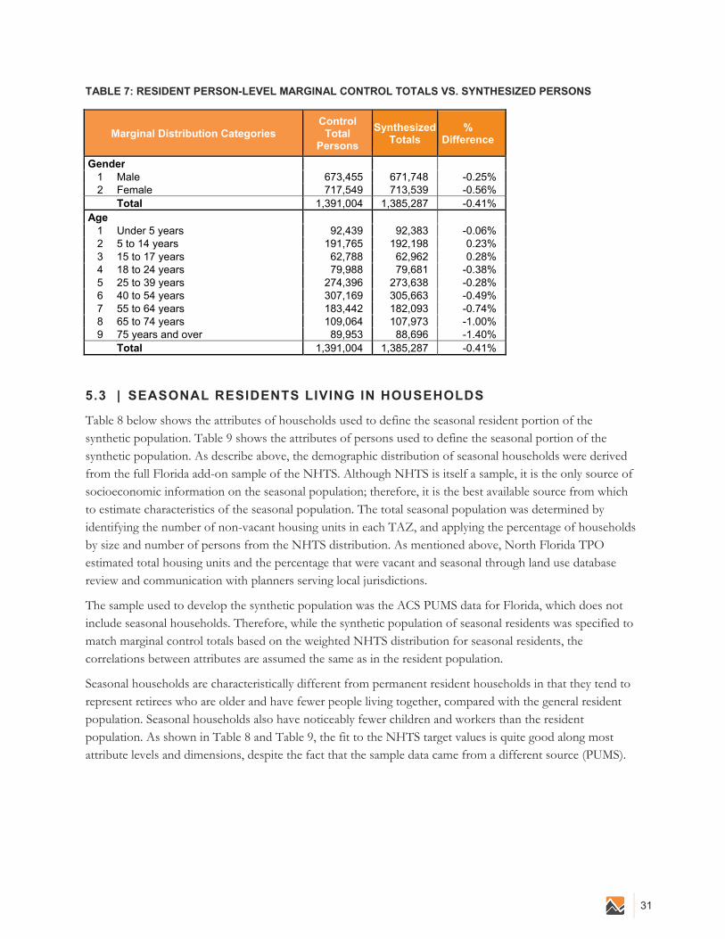
31
TABLE 7: RESIDENT PERSON-LEVEL MARGINAL CONTROL TOTALS VS. SYNTHESIZED PERSONS
Marginal Distribution Categories Control
Total Persons
SynthesizedTotals
% Difference
Gender 1 Male 673,455 671,748 -0.25% 2 Female 717,549 713,539 -0.56% Total 1,391,004 1,385,287 -0.41%
Age 1 Under 5 years 92,439 92,383 -0.06% 2 5 to 14 years 191,765 192,198 0.23% 3 15 to 17 years 62,788 62,962 0.28% 4 18 to 24 years 79,988 79,681 -0.38% 5 25 to 39 years 274,396 273,638 -0.28% 6 40 to 54 years 307,169 305,663 -0.49% 7 55 to 64 years 183,442 182,093 -0.74% 8 65 to 74 years 109,064 107,973 -1.00% 9 75 years and over 89,953 88,696 -1.40% Total 1,391,004 1,385,287 -0.41%
5.3 | SEASONAL RESIDENTS LIVING IN HOUSEHOLDS
Table 8 below shows the attributes of households used to define the seasonal resident portion of the synthetic population. Table 9 shows the attributes of persons used to define the seasonal portion of the synthetic population. As describe above, the demographic distribution of seasonal households were derived from the full Florida add-on sample of the NHTS. Although NHTS is itself a sample, it is the only source of socioeconomic information on the seasonal population; therefore, it is the best available source from which to estimate characteristics of the seasonal population. The total seasonal population was determined by identifying the number of non-vacant housing units in each TAZ, and applying the percentage of households by size and number of persons from the NHTS distribution. As mentioned above, North Florida TPO estimated total housing units and the percentage that were vacant and seasonal through land use database review and communication with planners serving local jurisdictions.
The sample used to develop the synthetic population was the ACS PUMS data for Florida, which does not include seasonal households. Therefore, while the synthetic population of seasonal residents was specified to match marginal control totals based on the weighted NHTS distribution for seasonal residents, the correlations between attributes are assumed the same as in the resident population.
Seasonal households are characteristically different from permanent resident households in that they tend to represent retirees who are older and have fewer people living together, compared with the general resident population. Seasonal households also have noticeably fewer children and workers than the resident population. As shown in Table 8 and Table 9, the fit to the NHTS target values is quite good along most attribute levels and dimensions, despite the fact that the sample data came from a different source (PUMS).

V 1.0 Northeast Regional Planning Model: Activity Based Calibration and Model Validation Report
32 February 12, 2015
TABLE 8: SEASONAL HOUSEHOLD-LEVEL MARGINAL CONTROL TOTALS VS. SYNTHESIZED HOUSEHOLDS
Marginal Distribution Categories Control
Total Households
Synthesized Totals
% Difference
Householder age 1 Householder 15 to 24 years 791 811 2.53% 2 Householder 25 to 54 years 1,819 1,717 -5.61% 3 Householder 55 to 64 years 3,604 3,647 1.19% 4 Householder 65 to 74 years 5,793 5,819 0.45% 5 Householder 75 years and over 4,847 4,860 0.27%
Total 16,854 16,854 0.00% Household size
1 1-person HH 3,675 3,688 0.35% 2 2-person HH 11,246 11,234 -0.11% 3 3-person HH 685 686 0.15% 4 4 or more-person HH 1,248 1,246 -0.16%
Total 16,854 16,854 0.00% Household unit type
1 SFD 11,707 11,701 -0.05% 2 MFD 5,147 5,153 0.12%
Total 16,854 16,854 0.00% Presence of household children
1 Yes 1,134 1,119 -1.32% 2 No 15,720 15,735 0.10%
Total 16,854 16,854 0.00% Family annual income
1 Less than $20,000 2,319 2,308 -0.47% 2 $20,000 to $39,999 4,828 4,848 0.41% 3 $40,000 to $59,999 2,461 2,455 -0.24% 4 $60,000 to $99,999 3,175 3,198 0.72% 5 $100,000 or more 4,071 4,045 -0.64%
Total 16,854 16,854 0.00% Persons by workers joint variable
1 1-persons, no worker 2,980 2,979 -0.03% 2 1-persons, 1 worker 695 695 0.00% 3 2-persons, no worker 9,156 9,138 -0.20% 4 2-persons, 1 worker 1,361 1,360 -0.07% 5 2-persons, 2 workers 729 729 0.00% 6 3-persons, no worker 37 38 2.70% 7 3-persons, 1 worker 416 420 0.96% 8 3-persons, 2 workers 232 233 0.43% 9 4 or more-persons, no worker 10 9 -10.00%
10 4 or more-persons, 1 worker 483 489 1.24% 11 4 or more-persons, 2 workers 17 16 -5.88% 12 4 or more-persons, 3 or more workers 738 748 1.36%
Total 16,854 16,854 0.00%

33
TABLE 9: SEASONAL PERSON-LEVEL MARGINAL CONTROL TOTALS VS. SYNTHESIZED PERSONS
Marginal Distribution Categories Control
Total Persons Synthesized
Totals % Difference
Gender 1 Male 16,670 17,125 2.73% 2 Female 18,005 17,438 -3.15%
Total 34,675 34,563 -0.32% Age
1 0 to 17 years 1,655 1,522 -8.04% 2 18 to 24 years 2,749 2,635 -4.15% 3 25 to 39 years 1,089 1,172 7.62% 4 40 to 54 years 4,355 4,352 -0.07% 5 55 to 64 years 6,235 6,285 0.80% 6 65 and 74 years 10,382 10,392 0.10% 7 75 years and over 8,210 8,205 -0.06%
Total 34,675 34,563 -0.32%
5.4 | GROUP QUARTERS RESIDENTS
Table 10 below shows the attributes of persons comprising the GQ portion of the synthetic population. This segment is the easiest to calibrate, because each GQ resident is modeled as a single-person household. There are only person-level controls, resulting in a near-perfect fit to the data, which were derived from Census blocks. Fewer age categories are used due to the relatively small sample size.
TABLE 10: GROUP QUARTERS PERSON-LEVEL MARGINAL CONTROL TOTALS VS. SYNTHESIZED PERSONS
Marginal Distribution Categories Control
Total Persons Synthesized
Totals % Difference
Gender 1 Male 12,925 12,927 0.0% 2 Female 15,403 15,401 0.0% Total 28,328 28,328 0.0%
Age 1 Under 18 years 655 655 0.0% 2 18 to 64 years 26,633 26,633 0.0% 3 65 years and over 1,040 1,040 0.0% Total 28,328 28,328 0.0%
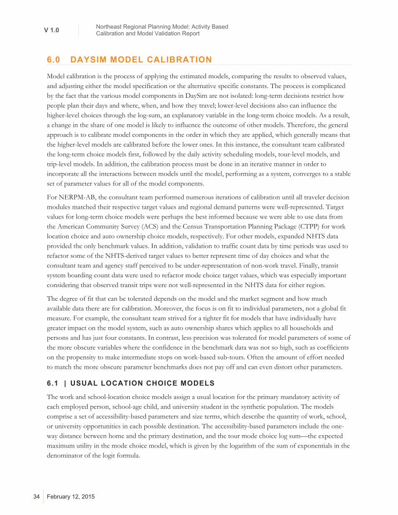
V 1.0 Northeast Regional Planning Model: Activity Based Calibration and Model Validation Report
34 February 12, 2015
6.0 DAYSIM MODEL CALIBRATION
Model calibration is the process of applying the estimated models, comparing the results to observed values, and adjusting either the model specification or the alternative specific constants. The process is complicated by the fact that the various model components in DaySim are not isolated: long-term decisions restrict how people plan their days and where, when, and how they travel; lower-level decisions also can influence the higher-level choices through the log-sum, an explanatory variable in the long-term choice models. As a result, a change in the share of one model is likely to influence the outcome of other models. Therefore, the general approach is to calibrate model components in the order in which they are applied, which generally means that the higher-level models are calibrated before the lower ones. In this instance, the consultant team calibrated the long-term choice models first, followed by the daily activity scheduling models, tour-level models, and trip-level models. In addition, the calibration process must be done in an iterative manner in order to incorporate all the interactions between models until the model, performing as a system, converges to a stable set of parameter values for all of the model components.
For NERPM-AB, the consultant team performed numerous iterations of calibration until all traveler decision modules matched their respective target values and regional demand patterns were well-represented. Target values for long-term choice models were perhaps the best informed because we were able to use data from the American Community Survey (ACS) and the Census Transportation Planning Package (CTPP) for work location choice and auto ownership choice models, respectively. For other models, expanded NHTS data provided the only benchmark values. In addition, validation to traffic count data by time periods was used to refactor some of the NHTS-derived target values to better represent time of day choices and what the consultant team and agency staff perceived to be under-representation of non-work travel. Finally, transit system boarding count data were used to refactor mode choice target values, which was especially important considering that observed transit trips were not well-represented in the NHTS data for either region.
The degree of fit that can be tolerated depends on the model and the market segment and how much available data there are for calibration. Moreover, the focus is on fit to individual parameters, not a global fit measure. For example, the consultant team strived for a tighter fit for models that have individually have greater impact on the model system, such as auto ownership shares which applies to all households and persons and has just four constants. In contrast, less precision was tolerated for model parameters of some of the more obscure variables where the confidence in the benchmark data was not so high, such as coefficients on the propensity to make intermediate stops on work-based sub-tours. Often the amount of effort needed to match the more obscure parameter benchmarks does not pay off and can even distort other parameters.
6.1 | USUAL LOCATION CHOICE MODELS
The work and school-location choice models assign a usual location for the primary mandatory activity of each employed person, school-age child, and university student in the synthetic population. The models comprise a set of accessibility-based parameters and size terms, which describe the quantity of work, school, or university opportunities in each possible destination. The accessibility-based parameters include the one-way distance between home and the primary destination, and the tour mode choice log sum—the expected maximum utility in the mode choice model, which is given by the logarithm of the sum of exponentials in the denominator of the logit formula.
35
The calibration of work location involved matching, by worker type, the observed origin-destination (OD) network distance frequency distributions from the 2010 NHTS. To achieve a good match, decision-makers’ disinclination toward distant locations was adjusted by changing the form of a piece-wise linear distance term in the utility function. Comparisons between observed and modeled OD distance frequency distributions for all work locations are shown in Figure 9.
FIGURE 9: WORK TRIP DISTANCE DISTRIBUTION COMPARISON
Table 11 below, shows the comparison of average commute trip distance, by worker type. Note that this is only for internal-internal commutes. Persons commuting into and out of the region for work are represented in the IE/EI trip tables. In addition to commute distance, county-to-county work flow is also calibrated against the American Community Survey (ACS) 2006–2010 five-year-average commute flow.
TABLE 11: COMPARISON OF AVERAGE COMMUTE TRIP, BY WORKER TYPE
WORKER TYPE NHTS (MILES) DAYSIM (MILES)
Full-Time Workers 12.94 13.83
Part-Time Workers 9.40 10.32
Student Workers 6.54 8.12
All Workers 12.01 12.91
The validation process found that the work-location choice model variables related to employment opportunities (attractors) and travel impedance did not explain all of the observed variation of work-location choice. This is a common phenomenon in all travel demand models; the consensus is that it represents an
0%
1%
2%
3%
4%
5%
6%
7%
8%
0 10 20 30 40 50 60 70 80 90
Miles
NHTS
DaySim

V 1.0 Northeast Regional Planning Model: Activity Based Calibration and Model Validation Report
36 February 12, 2015
orientation toward a local labor market. To address this, an intra-county bias factor was introduced to increase commute trips within the same county. Table 12 shows the distribution of county-to-county work commutes estimated by the model. Table 13 lists the intra-county bias factors for each county and their equivalent commute distance. For example, the intra-county bias factor in Baker County is 0.3, which suggests that Baker County residents would be willing to travel 0.07 miles farther to remain within the county than to commute out of Baker County to a location that might be closer. These are not strong bias factors, compared with other metropolitan areas, and in Putnam and St. John’s Counties no bias was detected. Table 14 shows the percentage difference of county-to-county worker flows of the calibrated model and the ACS 2006–2010 five-year average.
TABLE 12: DISTRIBUTION OF ESTIMATED WORK COMMUTE FLOWS, BY COUNTY
O/D Baker Clay Duval Nassau Putnam St. Johns Total Baker 55% 4% 39% 2% 0% 1% 100%
Clay 1% 49% 45% 1% 2% 3% 100%
Duval 0% 3% 92% 1% 0% 3% 100%
Nassau 1% 1% 42% 55% 0% 1% 100%
Putnam 0% 7% 6% 0% 80% 7% 100%
St. Johns 0% 4% 40% 0% 2% 54% 100%
Total 1% 9% 73% 4% 3% 9% 100%
TABLE 13: INTRA-COUNTY BIAS FACTOR
COUNTY INTRA-COUNTY BIAS FACTOR
EQUIVALENT ADDITIONAL COMMUTE
DISTANCE (MILES) Baker 0.30 0.07
Clay 0.65 0.15
Duval 0.25 0.06
Nassau 0.15 0.03
Putnam 0 N/A
St. Johns 0 N/A
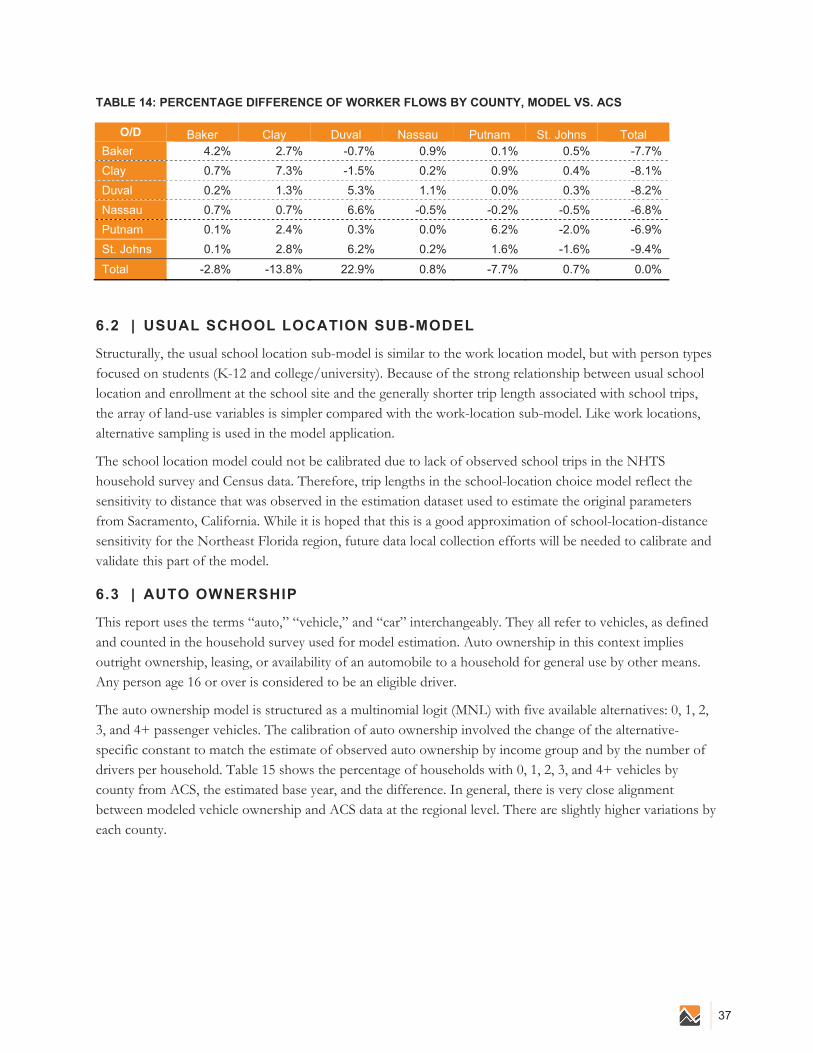
37
TABLE 14: PERCENTAGE DIFFERENCE OF WORKER FLOWS BY COUNTY, MODEL VS. ACS
O/D Baker Clay Duval Nassau Putnam St. Johns Total Baker 4.2% 2.7% -0.7% 0.9% 0.1% 0.5% -7.7%
Clay 0.7% 7.3% -1.5% 0.2% 0.9% 0.4% -8.1%
Duval 0.2% 1.3% 5.3% 1.1% 0.0% 0.3% -8.2%
Nassau 0.7% 0.7% 6.6% -0.5% -0.2% -0.5% -6.8%
Putnam 0.1% 2.4% 0.3% 0.0% 6.2% -2.0% -6.9%
St. Johns 0.1% 2.8% 6.2% 0.2% 1.6% -1.6% -9.4%
Total -2.8% -13.8% 22.9% 0.8% -7.7% 0.7% 0.0%
6.2 | USUAL SCHOOL LOCATION SUB-MODEL
Structurally, the usual school location sub-model is similar to the work location model, but with person types focused on students (K-12 and college/university). Because of the strong relationship between usual school location and enrollment at the school site and the generally shorter trip length associated with school trips, the array of land-use variables is simpler compared with the work-location sub-model. Like work locations, alternative sampling is used in the model application.
The school location model could not be calibrated due to lack of observed school trips in the NHTS household survey and Census data. Therefore, trip lengths in the school-location choice model reflect the sensitivity to distance that was observed in the estimation dataset used to estimate the original parameters from Sacramento, California. While it is hoped that this is a good approximation of school-location-distance sensitivity for the Northeast Florida region, future data local collection efforts will be needed to calibrate and validate this part of the model.
6.3 | AUTO OWNERSHIP
This report uses the terms “auto,” “vehicle,” and “car” interchangeably. They all refer to vehicles, as defined and counted in the household survey used for model estimation. Auto ownership in this context implies outright ownership, leasing, or availability of an automobile to a household for general use by other means. Any person age 16 or over is considered to be an eligible driver.
The auto ownership model is structured as a multinomial logit (MNL) with five available alternatives: 0, 1, 2, 3, and 4+ passenger vehicles. The calibration of auto ownership involved the change of the alternative-specific constant to match the estimate of observed auto ownership by income group and by the number of drivers per household. Table 15 shows the percentage of households with 0, 1, 2, 3, and 4+ vehicles by county from ACS, the estimated base year, and the difference. In general, there is very close alignment between modeled vehicle ownership and ACS data at the regional level. There are slightly higher variations by each county.

V 1.0 Northeast Regional Planning Model: Activity Based Calibration and Model Validation Report
38 February 12, 2015
TABLE 15: VEHICLE OWNERSHIP, BY COUNTY
ACS 2006–2010 FIVE-YEAR AVERAGE
COUNTY/CARS 0 1 2 3 4+ TOTAL
Baker 3% 33% 42% 16% 6% 100%
Clay 3% 27% 46% 18% 6% 100%
Duval 8% 38% 39% 11% 4% 100%
Nassau 5% 27% 42% 19% 7% 100%
Putnam 6% 39% 39% 12% 4% 100%
St. Johns 4% 31% 49% 12% 4% 100%
Region 6% 35% 41% 13% 4% 100%
ESTIMATED BASE–YEAR CONDITION
COUNTY/CARS 0 1 2 3 4+ TOTAL
Baker 4% 31% 45% 15% 6% 100%
Clay 3% 28% 46% 16% 6% 100%
Duval 8% 36% 39% 12% 4% 100%
Nassau 4% 31% 45% 14% 6% 100%
Putnam 5% 38% 41% 12% 5% 100%
St. Johns 4% 31% 46% 14% 5% 100%
Region 6% 34% 42% 13% 5% 100%
% DIFFERENCE
COUNTY/CARS 0 1 2 3 4+ TOTAL
Baker 0% -1% 2% -1% 0% 0%
Clay 1% 1% 1% -2% 0% 0%
Duval 0% -2% 0% 1% 1% 0%
Nassau -1% 4% 3% -5% -1% 0%
Putnam -1% -1% 1% 0% 1% 0%
St. Johns 0% 0% -3% 2% 0% 0%
Region 0% -1% 0% 0% 0% 0%
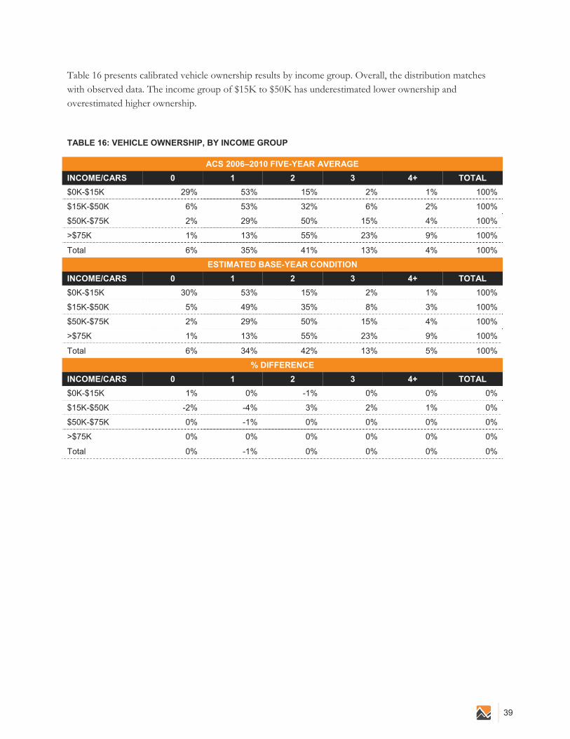
39
Table 16 presents calibrated vehicle ownership results by income group. Overall, the distribution matches with observed data. The income group of $15K to $50K has underestimated lower ownership and overestimated higher ownership.
TABLE 16: VEHICLE OWNERSHIP, BY INCOME GROUP
ACS 2006–2010 FIVE-YEAR AVERAGE
INCOME/CARS 0 1 2 3 4+ TOTAL
$0K-$15K 29% 53% 15% 2% 1% 100%
$15K-$50K 6% 53% 32% 6% 2% 100%
$50K-$75K 2% 29% 50% 15% 4% 100%
>$75K 1% 13% 55% 23% 9% 100%
Total 6% 35% 41% 13% 4% 100%
ESTIMATED BASE-YEAR CONDITION
INCOME/CARS 0 1 2 3 4+ TOTAL
$0K-$15K 30% 53% 15% 2% 1% 100%
$15K-$50K 5% 49% 35% 8% 3% 100%
$50K-$75K 2% 29% 50% 15% 4% 100%
>$75K 1% 13% 55% 23% 9% 100%
Total 6% 34% 42% 13% 5% 100%
% DIFFERENCE
INCOME/CARS 0 1 2 3 4+ TOTAL
$0K-$15K 1% 0% -1% 0% 0% 0%
$15K-$50K -2% -4% 3% 2% 1% 0%
$50K-$75K 0% -1% 0% 0% 0% 0%
>$75K 0% 0% 0% 0% 0% 0%
Total 0% -1% 0% 0% 0% 0%

V 1.0 Northeast Regional Planning Model: Activity Based Calibration and Model Validation Report
40 February 12, 2015
Table 17 presents calibrated vehicle ownership results by the number of potential drivers in each household. These results show a very close match between the estimated and observed shares of households in each category.
TABLE 17: VEHICLE OWNERSHIP, BY NUMBER OF POTENTIAL DRIVERS IN HOUSEHOLD
ACS 2006–2010 FIVE-YEAR AVERAGE
HH # OF POTENTIAL DRIVERS
0 1 2 3 4+ TOTAL
1 14% 71% 13% 1% 0% 100%
2 3% 19% 63% 12% 2% 100%
3 2% 13% 34% 40% 11% 100%
4+ 3% 7% 23% 28% 40% 100%
Total 6% 35% 41% 13% 4% 100%
ESTIMATED BASE-YEAR CONDITION
HH # OF POTENTIAL DRIVERS
0 1 2 3 4+ TOTAL
1 13% 72% 13% 1% 0% 100%
2 3% 19% 64% 12% 2% 100%
3 2% 13% 34% 40% 11% 100%
4+ 3% 7% 23% 28% 39% 100%
Total 6% 34% 42% 13% 5% 100%
% DIFFERENCE
HH # OF POTENTIAL DRIVERS
0 1 2 3 4+ TOTAL
1 0% 0% 0% 0% 0% 0%
2 0% 0% 0% 0% 0% 0%
3 0% 0% 1% 0% -1% 0%
4+ 0% 0% 0% 1% -1% 0%
Total 0% -1% 0% 0% 0% 0%

41
6.4 | DAY PATTERN MODELS
The Day Pattern models include two main models and two sub-models. The main models are:
1) main-pattern model; and
2) exact number of tours model.
The two sub-models are:
1) number and purpose of work-based sub-tours model; and
2) intermediate-stops model.
The two main models jointly predicted the number of home-based tours a person undertakes during a day for seven purposes, and the occurrence of additional stops during the day for the same seven purposes. The seven purposes are work, school, escort, personal business, shopping, meal, and social/recreational. The pattern choice is a function of many types of household and person characteristics, as well as land use and accessibility at the residence and, if relevant, the usual work location. The main pattern model predicts the occurrence of tours (0 or 1+) and extra stops (0 or 1+) for each purpose, and a simpler conditional model predicts the exact number of tours for each purpose.
MAIN-PATTERN MODEL
The “base alternative” in the main-pattern model is the “stay-at-home” alternative, where all 14 dependent variables are zero (no tours or stops are made). The main utility component for each purpose-specific tour or stop alternative is a vector of person-specific and household-specific characteristics and accessibility measures. Important behavioral traits of the main-pattern model include:
Many household and person variables have significant effects on the likelihood of participating in different types of activities in the day, and on whether those activities tend to be made on separate tours or as stops on complex tours.
The significant variables include employment status, student status, age group, income group, car availability, work-at-home dummy, gender, presence of children in different age groups, presence of other adults in the household, and family/non-family status.
For workers and students, the accessibility (mode-choice log sum) of predicted usual work and school locations is positively related to the likelihood of traveling to that activity on a given day.
For workers, the accessibility to retail and service locations on the way to and from work is positively related to the likelihood of making intermediate stops for various purposes.
EXACT NUMBER OF TOURS MODEL
A much simpler model specification was used to estimate models of the exact number of tours for any given purpose, conditional on making 1+ tours for that purpose. Compared to the main day-pattern model, the person and household variables have less influence, but the accessibility variables have relatively more influence. This result indicates that the small percentage of people who make multiple tours for any given purpose during a day tend to be those people who live in areas that best accommodate those tours. Other people will be more likely to participate in fewer activities and/or group their activities into fewer home-based tours.

V 1.0 Northeast Regional Planning Model: Activity Based Calibration and Model Validation Report
42 February 12, 2015
NUMBER AND PURPOSE OF WORK-BASED SUB-TOURS MODEL
For each home-based work tour predicted by the main pattern model and extra number of tours model, this model predicts the exact number and primary purpose of work-based sub-tours that originate from that tour. This model uses a stop/repeat structure, with eight possible alternatives: one (more) sub-tour for any of seven different activity purposes, or no (more) sub-tours—called the “quit” alternative. When the model is applied, the choice is repeated until the purpose of the third sub-tour or the quit alternative is chosen, whichever comes first. The model imposes a limit of three sub-tours because that is the maximum number observed from the estimation dataset.
For this model, the following activity schedule outcomes are known, including the:
Number and purpose of all home-based tours (from main pattern model and exact number of tours model);
Presence of stops and/or work-based sub-tours in the day pattern model, but not whether they are intermediate stops or sub-tours from the main pattern model. (In cases where the main pattern model determines that there are no stops or work-based sub-tours, then the work-based sub-tour model is not needed.); and
Purposes of stops and/or sub-tours (from main pattern model).
In a given choice case, a sub-tour purpose is available only if the pattern indicates that at least one intermediate stop or work-based sub-tour occurs for that purpose. In addition, education sub-tours are considered unavailable unless the person reported being a student.
NUMBER AND PURPOSE OF INTERMEDIATE STOPS
For each tour, once its destination, timing, and mode have been determined, the exact number of stops and their purposes is modeled for the half-tours leading to and from the tour destination. For each potential stop, the model predicts whether an intermediate stop occurs or not and, if so, its purpose. This repeats until the “quit” alternative is predicted, or five stops have been made, whichever occurs first. The five-stop limit arises because no half-tours in the estimation data have more than five intermediate stops. In model application, for the last modeled tour, the model is constrained to accomplish all intermediate stop activity purposes prescribed by the activity pattern model that have not yet been accomplished on other tours.
Intermediate stops are strongly conditioned by the outcome of the day activity pattern model, including the presence and purpose of tours and stops. Predicted characteristics of the tour and half-tour strongly affect the stop choices, including tour purpose and mode, type, timing, and time available for the half-tour. Outcomes of this model for higher-priority tours have significant effects. For example, once a stop purpose is determined the likelihood of another stop for that purpose drops considerably. Person type and presence of children each affect the likelihood and purpose of intermediate stops. Accessibility has a small, but measurable, effect related to the proximity of nearby activity opportunities, such as retail shopping. For auto-based modes, accessibility is measured by the aggregate intermediate stop log sum. For non-auto-based modes, stop tendency depends on street network connectivity and commercial employment density.

43
CALIBRATING DAY PATTERN MODELS
Calibration of the day pattern models involves adjustment of alternative-specific constants to match observed tour and trip rates. NHTS 2010 survey data was to be the basis for calibration target values; however, the consulting team found in this, and similar studies using the NHTS data sources, that reported non-work tour rates were much lower than expected. This initially resulted in unusually low network assignment results during off-peak times of day, compared with count data. Further, a comparison between NHTS non-work non-school tour rates and the AASHTO report, titled “Commuting in America 2013” estimated that commute trips constitute about 16% of total person trips, whereas commute trips comprised 24% of person trips reported in the NHTS household survey for the Jacksonville region.
To address the under-reporting issue, the NHTS-derived target values for non-work and non-school tour and trip purposes were inflated uniformly by 25%, a value that seemed to generate about the right level of total demand in network assignment when compared to highway and transit validation counts. In addition, the impact on the model was an increase in non-work and school tours and trips, such that work tours now comprise about 20% of all tour purposes and trips to work represent 16% of all out-of-home stops on a tour, which is consistent with the AASHTO report referenced above.
These “adjusted observed” tours and trips were used as the targets in the calibration process and are reflected in the day pattern tour and stop rates found in Table 18, which shows calibrated tours by purpose. These rates were applied to the main pattern model to increase the rate of making one or more tours of a particular type. Overall, the model generated 2% fewer tours than adjusted observed target values; however, the differences are surprisingly close given the uniform 25% adjustment.
TABLE 18: TOURS, BY PURPOSE
PURPOSE ADJUSTED
OBSERVED* MODELED DIFFERENCE % DIFFERENCE
Work 452,984 428,606 -24,378 -5%
School 208,032 210,342 2,310 1%
Escort 260,864 261,647 783 0%
Personal Bus. 246,416 258,598 12,182 5%
Shop 382,995 370,301 -12,694 -3%
Meal 135,888 128,881 -7,007 -5%
Soc./Rec. 462,915 432,182 -30,733 -7%
Work-Based 77,009 80,900 3,891 5%
Total 2,227,104 2,171,457 -55,647 -2%
* The observed tours from the NHTS survey data were inflated by 25% for non-work and non-school purposes to account for under-reporting of discretionary travel.

V 1.0 Northeast Regional Planning Model: Activity Based Calibration and Model Validation Report
44 February 12, 2015
TABLE 19: TOUR RATES, BY PURPOSE
PURPOSE ADJUSTED
OBSERVED* MODELED DIFFERENCE % DIFFERENCE
Work 0.34 0.32 -0.02 -5%
School 0.16 0.16 0.00 1%
Escort 0.20 0.20 0.00 0%
Personal Bus. 0.18 0.19 0.01 5%
Shop 0.29 0.28 -0.01 -3%
Meal 0.10 0.10 -0.01 -5%
Soc./Rec. 0.35 0.32 -0.02 -7%
Work-Based 0.06 0.06 0.00 5%
All Purposes 1.67 1.63 -0.04 -2%
* The observed tours from the NHTS survey data were inflated by 25% for non-work and non-school purposes to account for under-reporting of discretionary travel.
TABLE 20: EXACT NUMBER OF TOURS BY PURPOSE, GIVEN AT LEAST ONE IN DAY PATTERN
WORK OBSERVED MODELED DIFFERENCE
1 93.8% 93.6% -0.2%
2 6.1% 6.1% 0.0%
3+ 0.1% 0.3% 0.2%
SCHOOL OBSERVED MODELED DIFFERENCE
1 97.2% 95.2% -2.0%
2 2.8% 4.5% 1.7%
3+ 0.0% 0.4% 0.4%
ESCORT OBSERVED MODELED DIFFERENCE
1 65.5% 65.3% -0.2%
2 27.4% 29.1% 1.7%
3+ 7.2% 5.6% -1.5% PERSONAL BUSINESS
OBSERVED MODELED DIFFERENCE
1 90.4% 87.2% -3.3%
2 9.4% 11.4% 2.0%
3+ 0.2% 1.4% 1.2%
SHOP OBSERVED MODELED DIFFERENCE
1 90.9% 84.6% -6.3%
2 7.6% 13.5% 6.0%
3+ 1.6% 1.9% 0.3%
MEAL OBSERVED MODELED DIFFERENCE
1 96.4% 97.0% 0.6%
2 3.6% 3.0% -0.6%
3+ 0.0% 0.0% 0.0%
SOCIAL/REC OBSERVED MODELED DIFFERENCE
1 90.8% 91.7% 0.9%
2 8.0% 7.8% -0.2%
3+ 1.1% 0.5% -0.7%

45
For each person, if the main pattern model predicts at least one tour of a particular type, DaySim also predicts the exact number of tours made by a person in an average day. Table 20, below, shows the exact number of tours by purpose: 1 tour, 2 tours, or 3 and 3-plus tours. For all persons making work tours, 94% made one work tour, and about 6% made two work tours; few individuals make more than two work tours per day. In this instance, the model estimation closely matched observed data. For the school purpose, 97% of persons making school tours make one school tour per day, and 2.8% made more than one school tour. The model overestimated one-plus school tours by 1.7%.
For shopping tours, the model overestimated two-shopping tours by 2.4%. The model overestimated two and two-plus person business tours by 3.3%. For shopping tours, 90% of individuals only make one shopping tour in an average day, and this is the one tour purpose where DaySim is over-estimating the number. In addition, the majority of persons making meal tours make only one meal tour in an average day. For all purposes, the distribution of the exact number of tours differences are less than 5%, with the exception of shopping where the model over-predicts multi-stop tours by 6.3%.
For each work tour, DaySim also determines whether a work-based sub-tour is made or not. Table 21 shows the calibration of work-based sub-tours. For persons making work tours, 83% of individuals do not make sub-tours, and 17% of individuals make one or more than one sub-tours. In this instance also, the model results closely matched observed data.
TABLE 21: WORK-BASED SUB-TOURS CALIBRATION
WORK-BASED SUB-TOURS
OBSERVED MODELED DIFFERENCE
0 84.2% 81.8% -2.5%
1 15.2% 17.9% 2.7%
2 0.5% 0.3% -0.2%
3+ 0.0% 0.0% 0.0%
Total 100.0% 100.0% 0.0%
The day-pattern model also includes the number and purpose of intermediate stops. The model results also closely matched these observed data, with results detailed below in Table 22. Approximately 66% of tours do not include intermediate stops. Work and shopping tours are less likely to include intermediate stops, while school and escort tours are more likely to have intermediate stops. This suggests that people tend to conduct escort and school tours in concert with other activities in their daily schedule.

V 1.0 Northeast Regional Planning Model: Activity Based Calibration and Model Validation Report
46 February 12, 2015
TABLE 22: NUMBER OF INTERMEDIATE STOPS, BY TOUR PURPOSE
Observed
Stops Work School Escort Pers Bus Shop Meal SocRec Total
0 57.0% 65.3% 54.5% 66.9% 71.4% 74.4% 74.2% 65.8%
1 18.1% 22.1% 18.5% 17.7% 15.5% 18.0% 18.0% 18.1%
2 13.5% 4.5% 13.2% 9.1% 9.1% 5.3% 4.6% 8.9%
3 5.3% 5.9% 6.1% 4.6% 2.2% 0.5% 1.7% 3.8%
4 2.3% 1.6% 4.6% 1.0% 0.9% 1.2% 0.2% 1.6%
5 3.1% 0.6% 1.3% 0.6% 0.3% 0.3% 1.2% 1.3%
6+ 0.6% 0.0% 1.7% 0.0% 0.6% 0.3% 0.1% 0.5%
Model
Stops Work School Escort Pers Bus Shop Meal SocRec Total
0 48.1% 75.1% 53.5% 66.9% 62.8% 76.9% 76.7% 64.4%
1 24.4% 14.0% 24.3% 20.8% 23.3% 16.4% 15.7% 20.4%
2 14.0% 6.5% 12.2% 8.0% 9.3% 4.8% 5.2% 8.9%
3 7.1% 2.6% 5.6% 2.9% 3.0% 1.4% 1.7% 3.7%
4 3.4% 1.1% 2.6% 1.0% 1.1% 0.4% 0.6% 1.6%
5 1.7% 0.5% 1.1% 0.3% 0.4% 0.1% 0.2% 0.7%
6+ 1.3% 0.3% 0.8% 0.1% 0.1% 0.0% 0.1% 0.4%
% Difference
Stops Work School Escort Pers Bus Shop Meal SocRec Total
0 -8.9% 9.8% -1.0% 0.0% -8.5% 2.5% 2.5% -1.4%
1 6.3% -8.1% 5.8% 3.1% 7.8% -1.7% -2.3% 2.3%
2 0.5% 2.0% -1.0% -1.1% 0.2% -0.5% 0.5% 0.0%
3 1.8% -3.3% -0.5% -1.8% 0.8% 0.9% 0.0% -0.1%
4 1.1% -0.5% -2.1% -0.1% 0.1% -0.8% 0.3% -0.1%
5 -1.4% -0.2% -0.2% -0.3% 0.1% -0.2% -1.0% -0.7%
6+ 0.7% 0.3% -0.9% 0.1% -0.5% -0.3% 0.0% 0.0%
6.5 | NON-MANDATORY TOUR DESTINATION CHOICE
The non-mandatory tour destination choice model is a multinomial logit model that is used to choose the primary activity stop on a tour as a function of activity opportunities (represented by employment and/or households) and offset by travel impedance. Urban form accessibility variables also play a large role in the attractiveness of a destination.
The model calibration process revealed that the model overestimated the frequency of trips across the St. John’s River. This discrepancy was attributed to the geographic barrier effect of the river was not reflected in DaySim’s travel impedance factor. To address this issue, a river crossing penalty, by purpose, was introduced to reflect reluctance to cross a large river for non-mandatory purpose tours. Unlike intra-county bias factors, which encourage commuting within the same county, river-crossing penalties discourage travel across the river for particular purposes. Table 23 presents the river-crossing penalty value and equivalent-distance

47
penalty, by miles. For example, the calibrated river-crossing penalty suggests that crossing the river for an escort-activity purpose is equivalent to traveling an additional 0.89 miles. Table 24 displays the distribution of non-mandatory tour origins and destinations, by the east and west side of the river.
TABLE 23: RIVER-CROSSING PENALTY
PURPOSE RIVER-CROSSING
PENALTY
EQUIVALENT-DISTANCE PENALTY
(MILES)
Escort -0.8 0.89
Personal Business -0.8 0.74
Shop -0.8 0.96
Meal -0.8 0.56
Social/Recreational -0.8 0.61
TABLE 24: RIVER-CROSSING DISTRIBUTION, NHTS VS. MODEL
OBSERVED
WEST–WEST WEST–EAST EAST–WEST EAST–EAST TOTAL
Escort 46% 4% 2% 48% 100%
Person 41% 6% 3% 50% 100%
Shop 50% 2% 1% 47% 100%
Meal 44% 7% 1% 47% 100%
Social/Recreational 46% 5% 7% 42% 100%
ESTIMATED
WEST–WEST WEST–EAST EAST–WEST EAST–EAST TOTAL
Escort 50% 4% 4% 42% 100%
Person 49% 3% 3% 44% 100%
Shop 48% 5% 4% 43% 100%
Meal 49% 3% 2% 46% 100%
Social/Recreational 49% 3% 2% 46% 100%
% DIFFERENCE
WEST–WEST WEST–EAST EAST–WEST EAST–EAST TOTAL
Escort 4% 0% 2% -6% 0%
Person 8% -3% 0% -6% 0%
Shop -2% 3% 3% -4% 0%
Meal 4% -4% 1% -2% 0%
Social/Recreational 3% -2% -4% 4% 0%

V 1.0 Northeast Regional Planning Model: Activity Based Calibration and Model Validation Report
48 February 12, 2015
The calibration of the non-mandatory tour-choice model is intended to match general distribution of tour lengths found in the NHTS survey data. Here, tour-length refers to the one-way distance between the home anchor point and the location of the primary stop on the tour, which is identified by purpose in the figures and tables that follow.
FIGURE 10: ESCORT-TOUR LENGTH DISTRIBUTION, NHTS VS. DAYSIM
Figure 10 represents the calibrated escort-tour-length distribution compared to the NHTS. The observed average escort tour length is 5.46 miles, compared with the predicted average 5.69-mile escort-tour length.
Table 25 compares the distribution of county-to-county escort tours between the NHTS and DaySim predictions. Escort tours most often involves parents providing rides to children in the household and are closely associated with childrens’ school activities. For example, one household members trip to school is another household member’s escort trip. The NHTS data predicts a very strong intra-county pattern to escort trips. DaySim over-predicts inter-county escort trips, particularly to Duval County; however, the differences are relatively small.
0%
5%
10%
15%
20%
0 10 20 30 40 50 60Miles
NHTS
DaySim
NHTS: 5.46 miles DaySim: 5.69 miles

49
TABLE 25: COUNTY-TO-COUNTY ESCORT TOUR FLOW, NHTS VS. DAYSIM
NHTS
O/D BAKER CLAY DUVAL NASSAU PUTNAM ST.
JOHNS TOTAL
Baker 71% 0% 29% 0% 0% 0% 100%
Clay 0% 91% 5% 0% 3% 0% 100%
Duval 0% 2% 97% 0% 0% 1% 100%
Nassau 0% 0% 12% 88% 0% 0% 100%
Putnam 0% 0% 2% 0% 98% 0% 100%
St. Johns
0% 0% 15% 0% 0% 85% 100%
DAYSIM
O/D BAKER CLAY DUVAL NASSAU PUTNAM ST.
JOHNS TOTAL
Baker 80% 2% 18% 0% 0% 0% 100%
Clay 0% 82% 17% 0% 1% 0% 100%
Duval 0% 2% 96% 0% 0% 1% 100%
Nassau 0% 1% 22% 76% 0% 0% 100%
Putnam 0% 3% 1% 0% 96% 1% 100%
St. Johns
0% 1% 22% 0% 0% 77% 100%
% DIFFERENCE
O/D BAKER CLAY DUVAL NASSAU PUTNAM
ST. JOHNS
TOTAL
Baker 9% 2% -11% 0% 0% 0% 0%
Clay 0% -9% 11% 0% -3% 0% 0%
Duval 0% 1% -1% 0% 0% 0% 0%
Nassau 0% 1% 11% -12% 0% 0% 0%
Putnam 0% 3% -2% 0% -1% 1% 0%
St. Johns
0% 1% 7% 0% 0% -8% 0%
Figure 11 presents the calibrated personal business tour-length distribution compared to the NHTS. The average personal business tour length is 7.04 miles, according to the NHTS survey. DaySim predicted an average personal business tour length of 8.64 miles. Looking at the two distributions, the divergence would seem to be mainly for trips less than one mile, where the NHTS seems to indicate a much higher percentage. This is likely an artifact in the survey data coding that may not be realistic, as the shape of the DaySim distribution looks more plausible.
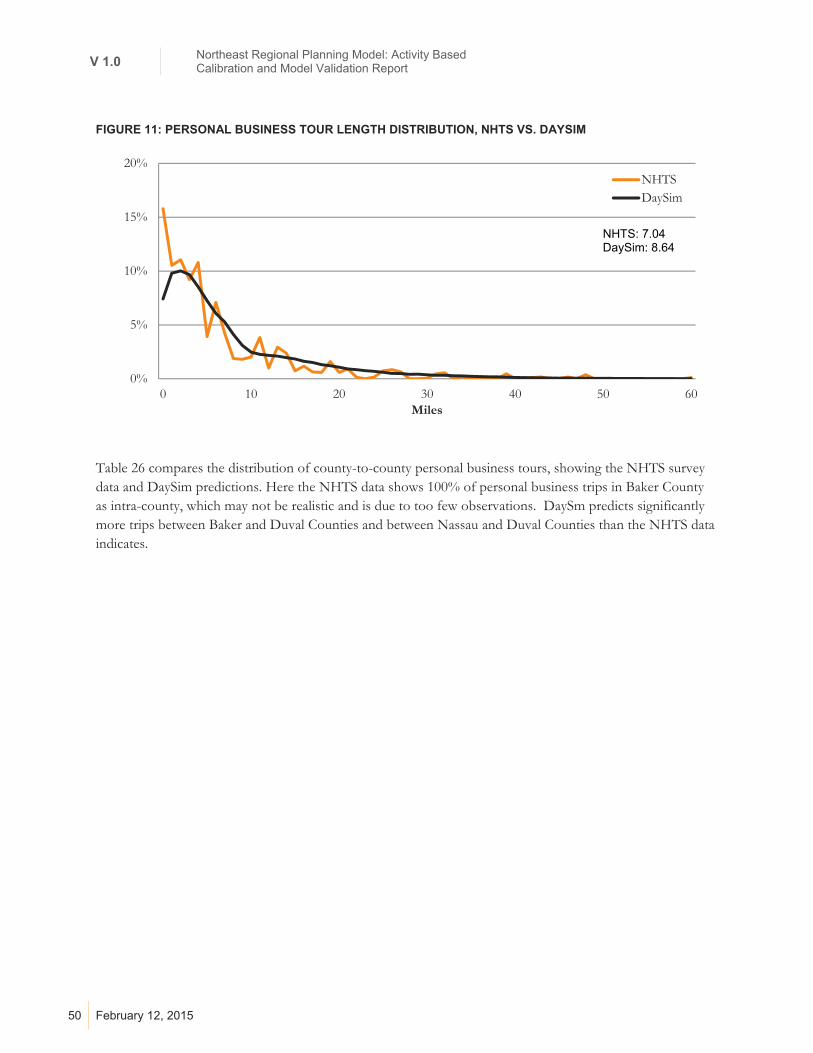
V 1.0 Northeast Regional Planning Model: Activity Based Calibration and Model Validation Report
50 February 12, 2015
FIGURE 11: PERSONAL BUSINESS TOUR LENGTH DISTRIBUTION, NHTS VS. DAYSIM
Table 26 compares the distribution of county-to-county personal business tours, showing the NHTS survey data and DaySim predictions. Here the NHTS data shows 100% of personal business trips in Baker County as intra-county, which may not be realistic and is due to too few observations. DaySm predicts significantly more trips between Baker and Duval Counties and between Nassau and Duval Counties than the NHTS data indicates.
0%
5%
10%
15%
20%
0 10 20 30 40 50 60Miles
NHTSDaySim
NHTS: 7.04 DaySim: 8.64

51
TABLE 26: COUNTY-TO-COUNTY PERSONAL BUSINESS TOUR FLOW, NHTS VS. DAYSIM
NHTS
O/D BAKER CLAY DUVAL NASSAU PUTNAM ST. JOHNS TOTAL
Baker 100% 0% 0% 0% 0% 0% 100%
Clay 0% 80% 20% 0% 0% 0% 100%
Duval 0% 1% 97% 0% 0% 2% 100%
Nassau 0% 0% 17% 83% 0% 0% 100%
Putnam 0% 0% 8% 0% 83% 9% 100%
St. Johns 0% 3% 18% 0% 0% 79% 100%
DAYSIM
O/D BAKER CLAY DUVAL NASSAU PUTNAM ST. JOHNS TOTAL
Baker 66% 4% 30% 0% 0% 0% 100%
Clay 0% 76% 22% 0% 1% 1% 100%
Duval 0% 3% 95% 0% 0% 1% 100%
Nassau 0% 2% 37% 61% 0% 0% 100%
Putnam 0% 5% 2% 0% 91% 2% 100%
St. Johns 0% 1% 27% 0% 0% 71% 100%
% DIFFERENCE
O/D BAKER CLAY DUVAL NASSAU PUTNAM ST. JOHNS TOTAL
Baker -34% 4% 30% 0% 0% 0% 0%
Clay 0% -4% 2% 0% 1% 1% 0%
Duval 0% 2% -2% 0% 0% -1% 0%
Nassau 0% 2% 20% -23% 0% 0% 0%
Putnam 0% 5% -7% 0% 8% -7% 0%
St. Johns 0% -2% 9% 0% 0% -7% 0%

V 1.0 Northeast Regional Planning Model: Activity Based Calibration and Model Validation Report
52 February 12, 2015
Figure 12 shows calibrated shopping tour length distribution compared to the NHTS. The average shopping tour length is 4.68 miles according to the NHTS survey, and DaySim predicted an average tour length of 4.59 miles.
FIGURE 12: SHOPPING TOUR LENGTH DISTRIBUTION, NHTS VS. DAYSIM
Table 27 compares the distribution of county-to-county tours reported by the NHTS and predicted by DaySim. There is a strong correspondence between the NHTS data and the modeled trip lengths, helped by a large number of observed shopping tours. Shopping tours for routine items, such as groceries, are often close to home, hence the larger proportion of intra-country tour destinations shown in the table.
0%
5%
10%
15%
20%
0 10 20 30 40 50 60Miles
NHTSDaySim
NHTS: 4.68
DaySim: 4.59

53
TABLE 27: COUNTY-TO-COUNTY SHOPPING TOUR FLOW, NHTS VS. DAYSIM
NHTS
O/D BAKER CLAY DUVAL NASSAU PUTNAM ST. JOHNS TOTAL
Baker 100% 0% 0% 0% 0% 0% 100%
Clay 0% 91% 9% 0% 0% 0% 100%
Duval 0% 3% 92% 4% 0% 0% 100%
Nassau 0% 2% 12% 85% 0% 0% 100%
Putnam 0% 0% 0% 0% 100% 0% 100%
St. Johns 0% 3% 17% 0% 0% 80% 100%
DAYSIM
O/D BAKER CLAY DUVAL NASSAU PUTNAM ST. JOHNS TOTAL
Baker 100% 0% 0% 0% 0% 0% 100%
Clay 0% 91% 8% 0% 0% 0% 100%
Duval 0% 2% 98% 0% 0% 0% 100%
Nassau 1% 0% 12% 87% 0% 0% 100%
Putnam 0% 5% 0% 0% 95% 0% 100%
St. Johns 0% 0% 16% 0% 0% 83% 100%
% DIFFERENCE
O/D BAKER CLAY DUVAL NASSAU PUTNAM ST. JOHNS TOTAL
Baker 0% 0% 0% 0% 0% 0% 0%
Clay 0% 1% -1% 0% 0% 0% 0%
Duval 0% -2% 5% -4% 0% 0% 0%
Nassau 1% -2% 0% 2% 0% 0% 0%
Putnam 0% 5% 0% 0% -5% 0% 0%
St. Johns 0% -2% -1% 0% 0% 3% 0%
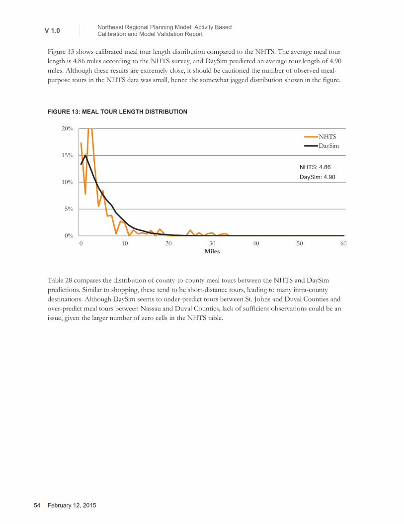
V 1.0 Northeast Regional Planning Model: Activity Based Calibration and Model Validation Report
54 February 12, 2015
Figure 13 shows calibrated meal tour length distribution compared to the NHTS. The average meal tour length is 4.86 miles according to the NHTS survey, and DaySim predicted an average tour length of 4.90 miles. Although these results are extremely close, it should be cautioned the number of observed meal-purpose tours in the NHTS data was small, hence the somewhat jagged distribution shown in the figure.
FIGURE 13: MEAL TOUR LENGTH DISTRIBUTION
Table 28 compares the distribution of county-to-county meal tours between the NHTS and DaySim predictions. Similar to shopping, these tend to be short-distance tours, leading to many intra-county destinations. Although DaySim seems to under-predict tours between St. Johns and Duval Counties and over-predict meal tours between Nassau and Duval Counties, lack of sufficient observations could be an issue, given the larger number of zero cells in the NHTS table.
0%
5%
10%
15%
20%
0 10 20 30 40 50 60Miles
NHTSDaySim
NHTS: 4.86
DaySim: 4.90

55
TABLE 28: COUNTY-TO-COUNTY MEAL TOUR FLOW, NHTS VS. DAYSIM
NHTS
O/D BAKER CLAY DUVAL NASSAU PUTNAM ST. JOHNS TOTAL
Baker 100% 0% 0% 0% 0% 0% 100%
Clay 0% 96% 4% 0% 0% 0% 100%
Duval 0% 1% 95% 0% 0% 4% 100%
Nassau 0% 0% 0% 100% 0% 0% 100%
Putnam 0% 6% 0% 0% 94% 0% 100%
St. Johns 0% 0% 37% 0% 5% 59% 100%
DAYSIM
O/D BAKER CLAY DUVAL NASSAU PUTNAM ST. JOHNS TOTAL
Baker 99% 0% 1% 0% 0% 0% 100%
Clay 0% 90% 10% 0% 0% 0% 100%
Duval 0% 2% 97% 0% 0% 1% 100%
Nassau 0% 0% 12% 88% 0% 0% 100%
Putnam 0% 4% 0% 0% 96% 0% 100%
St. Johns 0% 0% 14% 0% 0% 85% 100%
% DIFFERENCE
O/D BAKER CLAY DUVAL NASSAU PUTNAM ST. JOHNS TOTAL
Baker -1% 0% 1% 0% 0% 0% 0%
Clay 0% -6% 6% 0% 0% 0% 0%
Duval 0% 1% 2% 0% 0% -3% 0%
Nassau 0% 0% 12% -12% 0% 0% 0%
Putnam 0% -2% 0% 0% 2% 0% 0%
St. Johns 0% 0% -23% 0% -4% 27% 0%

V 1.0 Northeast Regional Planning Model: Activity Based Calibration and Model Validation Report
56 February 12, 2015
Figure 14 shows calibrated social and recreational tour length distribution compared to the NHTS. The average social and recreational tour length is 5.78 miles, according to the NHTS survey. DaySim predicted an average 5.04 miles of tour length. Despite these differences, the shapes of the two distributions track each other closely, thus DaySim provides a good approximation for to the more jagged NHTS distribution.
FIGURE 14: SOCIAL AND RECREATIONAL TOUR LENGTH DISTRIBUTION, NHTS VS. DAYSIM
Table 29 compares the distribution of county-to-county person tours between NHTS and DaySim predictions. One large error stands out—that the NHTS data predicts that half of the social and recreational tours originating in Baker County will be destined for Duval County. This proportion is quite large compared to the other counties, which tend to have a much higher proportion (90%) intra-county social/recreational tour destinations. Thus, this Baker County exception is likely the result of too few observations.
0%
5%
10%
15%
20%
0 10 20 30 40 50 60Miles
NHTSDaySim
NHTS: 5.78
DaySim: 5.04
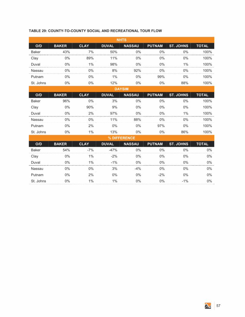
57
TABLE 29: COUNTY-TO-COUNTY SOCIAL AND RECREATIONAL TOUR FLOW
NHTS
O/D BAKER CLAY DUVAL NASSAU PUTNAM ST. JOHNS TOTAL
Baker 43% 7% 50% 0% 0% 0% 100%
Clay 0% 89% 11% 0% 0% 0% 100%
Duval 0% 1% 98% 0% 0% 1% 100%
Nassau 0% 0% 8% 92% 0% 0% 100%
Putnam 0% 0% 1% 0% 99% 0% 100%
St. Johns 0% 0% 12% 0% 0% 88% 100%
DAYSIM
O/D BAKER CLAY DUVAL NASSAU PUTNAM ST. JOHNS TOTAL
Baker 96% 0% 3% 0% 0% 0% 100%
Clay 0% 90% 9% 0% 0% 0% 100%
Duval 0% 2% 97% 0% 0% 1% 100%
Nassau 0% 0% 11% 88% 0% 0% 100%
Putnam 0% 2% 0% 0% 97% 0% 100%
St. Johns 0% 1% 13% 0% 0% 86% 100%
% DIFFERENCE
O/D BAKER CLAY DUVAL NASSAU PUTNAM ST. JOHNS TOTAL
Baker 54% -7% -47% 0% 0% 0% 0%
Clay 0% 1% -2% 0% 0% 0% 0%
Duval 0% 1% -1% 0% 0% 0% 0%
Nassau 0% 0% 3% -4% 0% 0% 0%
Putnam 0% 2% 0% 0% -2% 0% 0%
St. Johns 0% 1% 1% 0% 0% -1% 0%

V 1.0 Northeast Regional Planning Model: Activity Based Calibration and Model Validation Report
58 February 12, 2015
6.6 | TOUR MODE CHOICE
Tour main mode is the predominant mode chosen for making a given tour, based on the pseudo trip between the home end of the tour and the chosen primary activity destination. The actual mode chosen for each segment of the tour is modeled as “trip mode” at a lower level, but is strongly conditioned by the choice of a tour mode. The relationship between tour main mode and trip mode for trips within a single tour—and for a given person—is analogous to usual work and school location, and work and tour destination (i.e., the higher-level choice is highly determinative of the lower-level choice). The predominant mode chosen for a tour is the most likely mode for each segment within that tour.
The tour main mode sub-model is structured as a multinomial logit with the following eight mode options:
Drive-to-transit: Available only in the Home-based Work model, for tours with a valid drive to transit path in both the outbound and return observed tour.
Walk-to-transit: Available in all models except for Home-based Escort, for tours with a valid walk-to-transit path in both the outbound and return observed tour periods.
School bus: Available only in the Home-based School model, for all tours. Shared Ride (3 or more persons): Available in all models, for all tours. Shared Ride (2 persons): Available in all models, for all tours. Drive Alone: Available in all models except for Home-based Escort, for tours made by persons age
16+ in car-owning households. Bicycle: Available in all models except for Home-based Escort, for all tours with roundtrip road
distance of 30 miles or less. This was the threshold used when these models were estimated. The probability of the model predicting bicycle trips longer than 15 miles is extremely small.
Walk: Available in all models, for all tours with roundtrip road distance of 10 miles or less. This was the threshold used when these models were estimated. The probability of the model predicting bicycle trips longer than 3 miles is extremely small.
There are five tour mode choice sub-models:
1) work tour;
2) school tour;
3) escort tour;
4) other-non-mandatory tour; and
5) work-based sub-tours.
Tour mode choice models are calibrated for each sub-model.
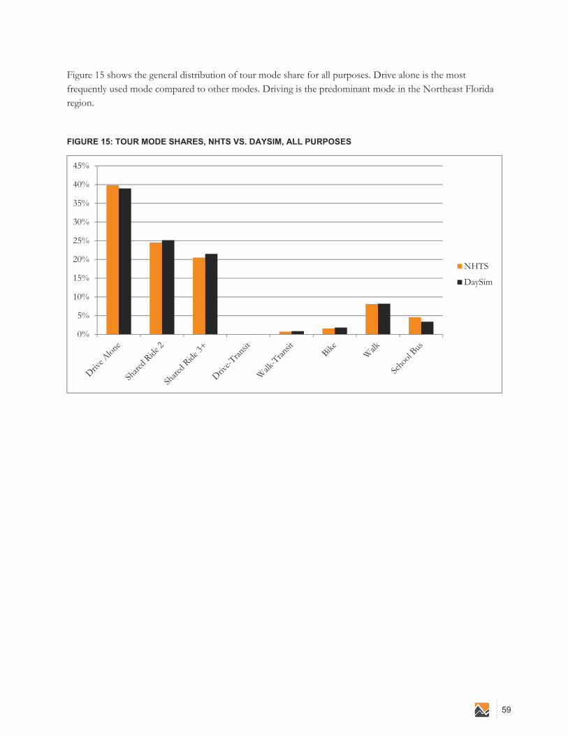
59
Figure 15 shows the general distribution of tour mode share for all purposes. Drive alone is the most frequently used mode compared to other modes. Driving is the predominant mode in the Northeast Florida region.
FIGURE 15: TOUR MODE SHARES, NHTS VS. DAYSIM, ALL PURPOSES
0%
5%
10%
15%
20%
25%
30%
35%
40%
45%
NHTS
DaySim

V 1.0 Northeast Regional Planning Model: Activity Based Calibration and Model Validation Report
60 February 12, 2015
Figure 16 shows the calibrated work tour mode results. The primary mode is drive alone, with over 70%. The majority of commuting trips are by driving. NHTS reported a small fraction of commuting trips by school bus. DaySim limited school bus mode for school tour only and therefore predicted no work tour modes by school bus.
FIGURE 16: WORK TOUR MODE SHARES, NHTS VS. DAYSIM
0%
10%
20%
30%
40%
50%
60%
70%
80%
NHTS
DaySim

61
Figure 17 shows the calibrated school tour mode results. Unlike the work tour mode, the primary mode in the school tour is school bus, followed by shared ride 3+.
FIGURE 17: SCHOOL TOUR MODE SHARES, NHTS VS. DAYSIM
0%
5%
10%
15%
20%
25%
30%
35%
40%
NHTS
DaySim

V 1.0 Northeast Regional Planning Model: Activity Based Calibration and Model Validation Report
62 February 12, 2015
Figure 18 shows the calibrated escort tour mode results. Due to the feature of escort tour, primary tour modes are Shared ride 2 or 3+. Note that the NHTS data included some escort tours that were coded as using drive alone, as well as bike, walk and school bus. DaySim does not allow drive alone or school bus on an escort tour.
FIGURE 18: ESCORT TOUR MODE SHARES, NHTS VS. DAYSIM
0%
10%
20%
30%
40%
50%
60%
NHTS
DaySim
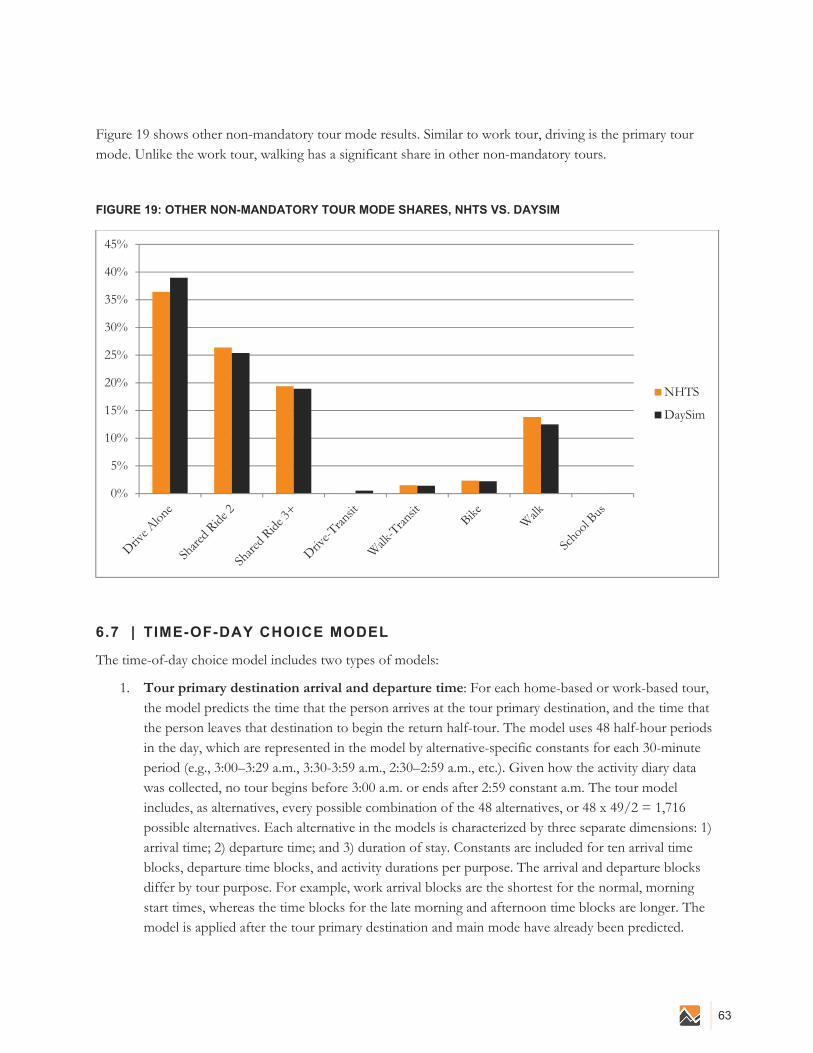
63
Figure 19 shows other non-mandatory tour mode results. Similar to work tour, driving is the primary tour mode. Unlike the work tour, walking has a significant share in other non-mandatory tours.
FIGURE 19: OTHER NON-MANDATORY TOUR MODE SHARES, NHTS VS. DAYSIM
6.7 | TIME-OF-DAY CHOICE MODEL
The time-of-day choice model includes two types of models:
1. Tour primary destination arrival and departure time: For each home-based or work-based tour, the model predicts the time that the person arrives at the tour primary destination, and the time that the person leaves that destination to begin the return half-tour. The model uses 48 half-hour periods in the day, which are represented in the model by alternative-specific constants for each 30-minute period (e.g., 3:00–3:29 a.m., 3:30-3:59 a.m., 2:30–2:59 a.m., etc.). Given how the activity diary data was collected, no tour begins before 3:00 a.m. or ends after 2:59 constant a.m. The tour model includes, as alternatives, every possible combination of the 48 alternatives, or 48 x 49/2 = 1,716 possible alternatives. Each alternative in the models is characterized by three separate dimensions: 1) arrival time; 2) departure time; and 3) duration of stay. Constants are included for ten arrival time blocks, departure time blocks, and activity durations per purpose. The arrival and departure blocks differ by tour purpose. For example, work arrival blocks are the shortest for the normal, morning start times, whereas the time blocks for the late morning and afternoon time blocks are longer. The model is applied after the tour primary destination and main mode have already been predicted.
0%
5%
10%
15%
20%
25%
30%
35%
40%
45%
NHTS
DaySim

V 1.0 Northeast Regional Planning Model: Activity Based Calibration and Model Validation Report
64 February 12, 2015
2. Intermediate stop arrival or departure time: For each intermediate stop made on any tour, this model predicts either the time that the person arrives at the stop location (on the first half tour), or the time that the person departs from the stop location (on the second half tour). On the second (return) half tour, the time that the person departs from the tour primary destination is known. Because the model is applied after the stop location and trip mode have been predicted, the travel time from the primary destination to the first intermediate stop is also known. As a result, the arrival time at the first intermediate stop is also known. So the model only needs to predict the departure time of the intermediate stop from among a maximum of 48 alternatives (the same 30-minute periods that are used in the tour models). This procedure is repeated for each intermediate stop on the half tour. On the first (outbound) half tour, the stops are simulated in reverse order from the primary destination back to the tour origin, so the departure time from each stop is known and the arrival time needs to be predicted.
In addition to the time-block constants, arrival and departure time choice models include other variables:
“Shift” Variables by Person Type: These variables effectively adjust the time block constants for arrival or duration by person type. For example, part-time workers and student workers tend to start work activities later than full-time workers; therefore, the shift constant for arrival time for part-time workers is positive, indicating later arrivals. Negative-sign shift coefficients arrive earlier, or participate in the activity for a shorter duration, than other person types; positive-sign shift coefficients arrive later or participate longer.
“Shift” Variables by Tour Complexity: Some shift variables account for complexity of tours, either by quantifying the numbers of stops for tours of different types, or the number of tours.
Income Variables: Lower-income workers tend to work for shorter durations, and higher-income workers tend to work longer hours.
Purpose-Specific Variables: Arrival and duration shift variables are included to differentiate each purpose, especially for the non-mandatory-purpose sub-model.
Time Pressure/Constraint Variables: Several variables were used to represent the constraints imposed on scheduling by inclusion of longer activities in a daily pattern, or by overall schedule complexity (e.g., number of tours and number of stops on tours).
Level of Service and Congestion Variables: Auto and transit travel time enters the model, along with the time spent in severe congestion. For purposes of the estimation, the marginal skims for the i-j TAZ interchange were used instead of surveyed information about the path taken for the trip.
Major effects captured in the models include:
Work Activities and Tours
Lower-income workers tend to have shorter-duration activities, and higher-income workers tend to have longer activities.
The more work-based sub-tours that are part of the tour, the longer the total duration of the work activity (including the sub-tour).
Workers making more intermediate stops to/from primary destination reduce the time spent at the primary activity.
Workers with 2+ tours to schedule will tend to try to leave a large consecutive block of time rather than two or more smaller blocks.

65
For both a.m. and p.m., workers tend to move the work activity earlier as the time in congested conditions increases.
School Activities and Tours
Many time pressure/constraint effects are similar to work activities and tours.
Non-Mandatory Activities and Tours
Relative to personal-business activities, people tend to arrive earlier for escort activities and later for shopping, meal, and social/recreation activities.
Escort and shopping activities also tend to be shorter in duration, while social/recreation activities tend to be longer.
Escort and shopping activities are likely to last less than one hour, and shopping and meal activities are likely to last 1-2 hours.
Shopping activities are unlikely to begin before 7:00 a.m. or end after 9:00 p.m. Meal activities are also unlikely to end after 9:00 p.m.
Escort activities are likely to end after 9:00 p.m. Time pressure/constraint effects are similar to those found for work and school tours. The main
difference is that the overall time pressure effect is stronger, but the other effects are weaker, and there is evidence that people will try to space tours more evenly during the day.
The p.m. peak was found to shift both earlier and later with high congestion.
Work-Based Activities and Tours
Escort, meal, and shopping activities tend to start later and be of shorter duration, relative to work-related activities on sub-tours.
Social/recreation activities also tend to start later, while personal business activities are also of shorter duration.
People try to leave consecutive windows both before and after the tour, meaning a tendency to “center” the sub-tour during the duration of the work activity.
Intermediate Stop Activities and Tours
Compared to work-related activities, stops for escort, shopping, meal, and personal business activities are of a shorter duration.
Escort, shopping, social/recreation, and personal business stops occur somewhat later in the day. These results are similar to those in the work- based sub-tour model.
Stops will tend to be shorter when there are more tours to be scheduled in the day, and also when are there more stops to be scheduled on the half tour. Figure 20 through Figure 23 show the distribution of observed arrival times at the tour primary destination, by tour purpose. School has the highest peak at 8:00 a.m. Work also has a peak at around 8:00 a.m. Non-mandatory activities are spread fairly evenly across the day. Most work-based tours begin near typical lunchtimes.
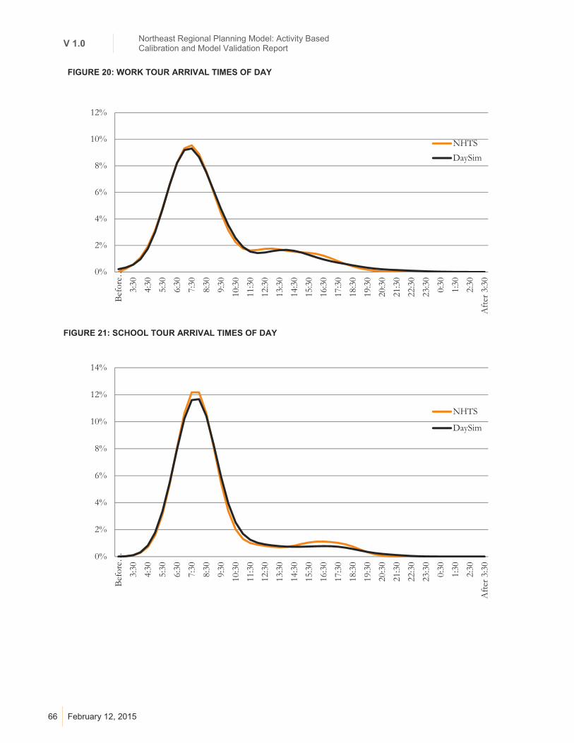
V 1.0 Northeast Regional Planning Model: Activity Based Calibration and Model Validation Report
66 February 12, 2015
FIGURE 20: WORK TOUR ARRIVAL TIMES OF DAY
FIGURE 21: SCHOOL TOUR ARRIVAL TIMES OF DAY
0%
2%
4%
6%
8%
10%
12%B
efor
e…
3:30
4:30
5:30
6:30
7:30
8:30
9:30
10:3
0
11:3
0
12:3
0
13:3
0
14:3
0
15:3
0
16:3
0
17:3
0
18:3
0
19:3
0
20:3
0
21:3
0
22:3
0
23:3
0
0:30
1:30
2:30
Aft
er 3
:30
NHTS
DaySim
0%
2%
4%
6%
8%
10%
12%
14%
Bef
ore…
3:30
4:30
5:30
6:30
7:30
8:30
9:30
10:3
0
11:3
0
12:3
0
13:3
0
14:3
0
15:3
0
16:3
0
17:3
0
18:3
0
19:3
0
20:3
0
21:3
0
22:3
0
23:3
0
0:30
1:30
2:30
Aft
er 3
:30
NHTS
DaySim

67
FIGURE 22: NON-MANDATORY TOUR ARRIVAL TIMES OF DAY
FIGURE 23: WORK-BASED SUB-TOUR ARRIVAL TIMES OF DAY
Figure 24 through Figure 27 show the distribution of departure times from tour primary activities. Note that non-mandatory and work-based sub-tours are similar for all purposes except work and school, indicating that
0.0%
0.5%
1.0%
1.5%
2.0%
2.5%
3.0%
3.5%
4.0%
4.5%B
efor
e…
3:30
4:30
5:30
6:30
7:30
8:30
9:30
10:3
0
11:3
0
12:3
0
13:3
0
14:3
0
15:3
0
16:3
0
17:3
0
18:3
0
19:3
0
20:3
0
21:3
0
22:3
0
23:3
0
0:30
1:30
2:30
Aft
er 3
:30
NHTS
DaySim
0%
2%
4%
6%
8%
10%
12%
14%
Bef
ore
3:00
am 3:30
4:30
5:30
6:30
7:30
8:30
9:30
10:3
0
11:3
0
12:3
0
13:3
0
14:3
0
15:3
0
16:3
0
17:3
0
18:3
0
19:3
0
20:3
0
21:3
0
22:3
0
23:3
0
0:30
1:30
2:30
Aft
er 3
:30
NHTS
DaySim

V 1.0 Northeast Regional Planning Model: Activity Based Calibration and Model Validation Report
68 February 12, 2015
those activities tend to be of a shorter duration, with similar start and end times. This is confirmed by Figure 28 through Figure 31, which show duration of stay at the tour destination. The work departure has peak at 5:00 p.m., and school departure has peak at 2:00 p.m. Non-mandatory activities are spread evenly across the afternoon. Most work-based tours end after lunch.
FIGURE 24: WORK-TOUR DEPART TIMES OF DAY
FIGURE 25: SCHOOL-TOUR DEPART TIMES OF DAY
0%
1%
2%
3%
4%
5%
6%
7%
8%
9%
10%
Bef
ore…
3:30
4:30
5:30
6:30
7:30
8:30
9:30
10:3
0
11:3
0
12:3
0
13:3
0
14:3
0
15:3
0
16:3
0
17:3
0
18:3
0
19:3
0
20:3
0
21:3
0
22:3
0
23:3
0
0:30
1:30
2:30
Aft
er 3
:30
NHTS
DaySim
0%
2%
4%
6%
8%
10%
12%
14%
Bef
ore…
3:30
4:30
5:30
6:30
7:30
8:30
9:30
10:3
0
11:3
0
12:3
0
13:3
0
14:3
0
15:3
0
16:3
0
17:3
0
18:3
0
19:3
0
20:3
0
21:3
0
22:3
0
23:3
0
0:30
1:30
2:30
Aft
er 3
:30
NHTS
DaySim

69
FIGURE 26: NON-MANDATORY-TOUR DEPARTURE TIMES OF DAY
FIGURE 27: WORK-BASED SUB-TOUR DEPARTURE TIMES OF DAY
Figure 28 through Figure 31 show the duration distribution for intermediate stops by activity purpose at the stop. In general, intermediate stops are of shorter duration than activities at primary destinations. This is partly by definition, since the rule for determining primary destination uses both activity purpose and duration. In general, work-related stops have the longest duration.
0.0%
0.5%
1.0%
1.5%
2.0%
2.5%
3.0%
3.5%
4.0%
4.5%B
efor
e…
3:30
4:30
5:30
6:30
7:30
8:30
9:30
10:3
0
11:3
0
12:3
0
13:3
0
14:3
0
15:3
0
16:3
0
17:3
0
18:3
0
19:3
0
20:3
0
21:3
0
22:3
0
23:3
0
0:30
1:30
2:30
Aft
er 3
:30
NHTS
DaySim
0%
2%
4%
6%
8%
10%
12%
Bef
ore
3:00
am 3:30
4:30
5:30
6:30
7:30
8:30
9:30
10:3
0
11:3
0
12:3
0
13:3
0
14:3
0
15:3
0
16:3
0
17:3
0
18:3
0
19:3
0
20:3
0
21:3
0
22:3
0
23:3
0
0:30
1:30
2:30
Aft
er 3
:30
NHTS
DaySim
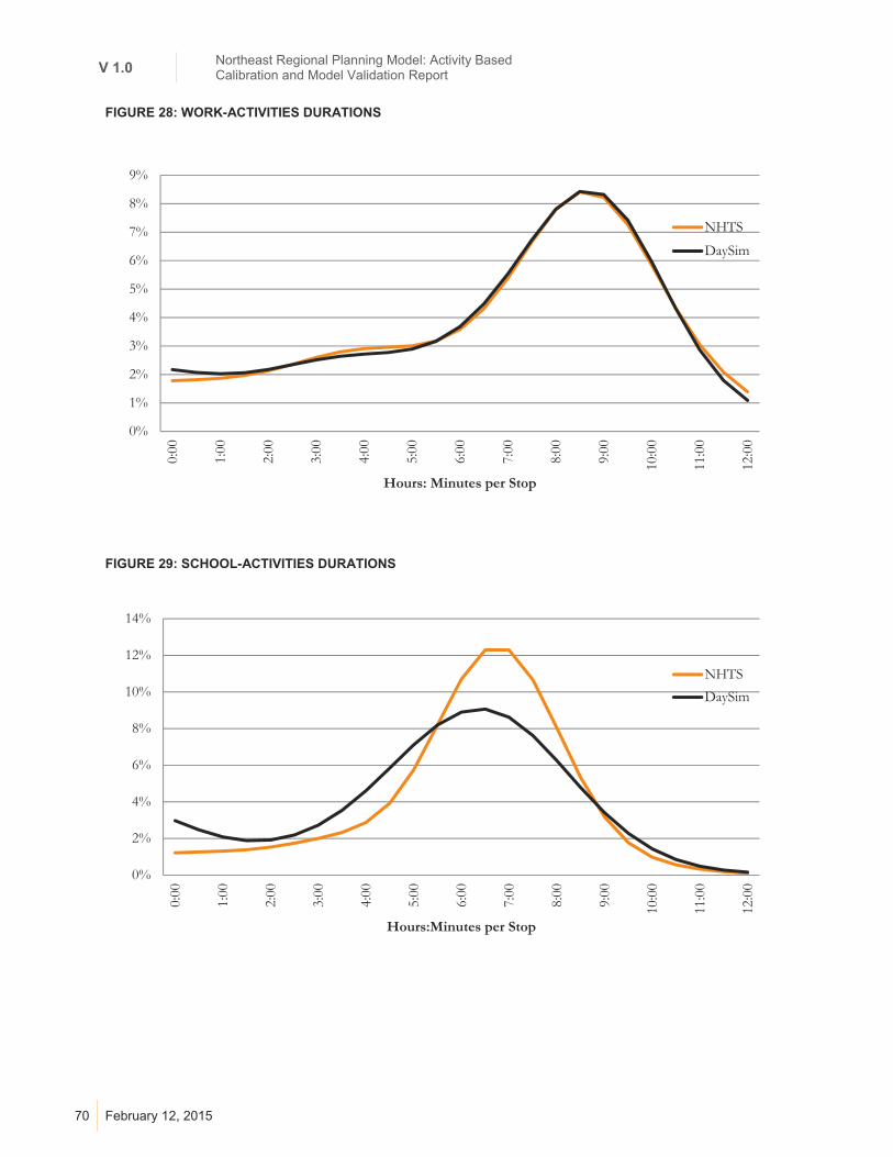
V 1.0 Northeast Regional Planning Model: Activity Based Calibration and Model Validation Report
70 February 12, 2015
FIGURE 28: WORK-ACTIVITIES DURATIONS
FIGURE 29: SCHOOL-ACTIVITIES DURATIONS
0%
1%
2%
3%
4%
5%
6%
7%
8%
9%0:
00
1:00
2:00
3:00
4:00
5:00
6:00
7:00
8:00
9:00
10:0
0
11:0
0
12:0
0
Hours: Minutes per Stop
NHTS
DaySim
0%
2%
4%
6%
8%
10%
12%
14%
0:00
1:00
2:00
3:00
4:00
5:00
6:00
7:00
8:00
9:00
10:0
0
11:0
0
12:0
0
Hours:Minutes per Stop
NHTS
DaySim
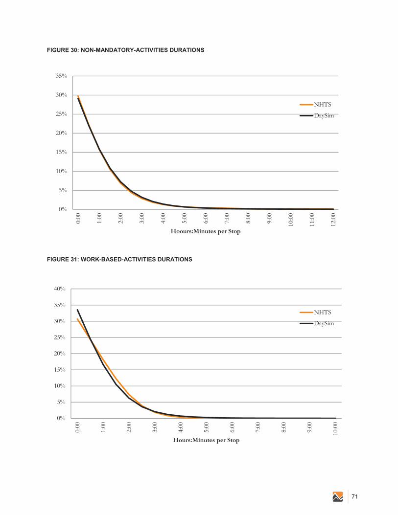
71
FIGURE 30: NON-MANDATORY-ACTIVITIES DURATIONS
FIGURE 31: WORK-BASED-ACTIVITIES DURATIONS
0%
5%
10%
15%
20%
25%
30%
35%0:
00
1:00
2:00
3:00
4:00
5:00
6:00
7:00
8:00
9:00
10:0
0
11:0
0
12:0
0
Hoours:Minutes per Stop
NHTS
DaySim
0%
5%
10%
15%
20%
25%
30%
35%
40%
0:00
1:00
2:00
3:00
4:00
5:00
6:00
7:00
8:00
9:00
10:0
0
Hours:Minutes per Stop
NHTS
DaySim

V 1.0 Northeast Regional Planning Model: Activity Based Calibration and Model Validation Report
72 February 12, 2015
7.0 NETWORK MODEL VALIDATION
7.1 | HIGHWAY ASSIGNMENT
For NERPM-AB, a number of coding changes were made to the existing NERPM v4.2 highway network to improve realism and the performance of the highway assignment model. Several ad hoc changes were made to correct miscoded attributes and to provide more realistic TAZ connectivity through the placement of connector links; however, three major efforts led to significant improvements in validation performance.
The most sweeping change was a network-wide re-calculation of link lengths, using ArcGIS, to measure distances more accurately. This was deemed necessary based on comparisons with GIS networks that showed significant discrepancies for certain facilities. Next was removal of ad hoc link speed penalties that were no longer necessary to compensate for inaccurate distances.
A river-crossing bias-parameter was added to the DaySim tour destination choice models for non-work and non-school purposes to improve cutline performance. As has been found in many other regions, travelers exhibit an aversion to major bridge crossings which is not adequately explained by differences in travel times and costs alone. If not accounted for, this can lead to over assignment of these facilities and incorrect OD patterns. This most notably affects trip purposes for discretionary purposes such as shopping, personal business, eating, social and recreation.
Speeds on surface arterials in Downtown Jacksonville were slowed to discourage unrealistic “cut through” movements, based on comparisons of routing using Google Maps ®. Links in the central business district (CBD) with coded Area Type 11 and arterial, collector and one-way facility types, were given free-flow speeds of 10 mph. This change reflects the fact that the CBD contains more closely spaced signalized intersections and slower corridor progression than other places in the region with the same area and facility type codes. The links had previously been coded with free-flow speeds of 25 and 35 mph and were not affected by any junction delay. Coded speeds for these same area and facility types were not changed outside of the Jacksonville CBD.
Free-flow speeds on freeways, Facility Types 11 and 12 in Area Types 2 and 3, fringe and residential, which had been coded with free-flow speeds of 75 mph, where reduced to 70 mph. This measure was taken to reduce system-wide over-assignment and is consistent with maximum, posted speed limits in these areas. Freeways free-flows speeds of 72.5 and 75 mph in rural area types were left unchanged.
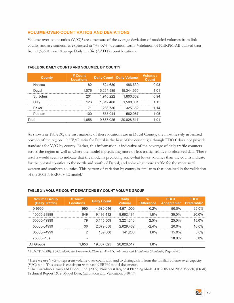
73
VOLUME-OVER-COUNT RATIOS AND DEVIATIONS
Volume-over-count ratios (V/G)4 are a measure of the average deviation of modeled volumes from link counts, and are sometimes expressed in “+/-X%” deviation form. Validation of NERPM-AB utilized data from 1,656 Annual Average Daily Traffic (AADT) count locations.
TABLE 30: DAILY COUNTS AND VOLUMES, BY COUNTY
County # Count
Locations Daily Count Daily Volume
Volume / Count
Nassau 82 524,630 486,630 0.93
Duval 1,076 15,264,985 15,344,965 1.01
St. Johns 201 1,910,222 1,800,302 0.94
Clay 126 1,312,408 1,508,001 1.15
Baker 71 286,736 325,652 1.14
Putnam 100 538,044 562,967 1.05
Total 1,656 19,837,025 20,028,517 1.01
As shown in Table 30, the vast majority of these locations are in Duval County, the most heavily urbanized portion of the region. The V/G ratio for Duval is the best of the counties; although FDOT does not provide standards for V/G by county. Rather, this information is indicative of the coverage of daily traffic counters across the region as well as where the model is predicting more or less traffic, relative to observed data. These results would seem to indicate that the model is predicting somewhat lower volumes than the counts indicate for the coastal counties to the north and south of Duval, and somewhat more traffic for the more rural western and southern counties. This pattern of variation by county is similar to that obtained in the validation of the 2005 NERPM v4.2 model.5
TABLE 31: VOLUME-COUNT DEVIATIONS BY COUNT VOLUME GROUP
Volume Group (Daily Traffic)
# Count Locations
Daily Count Daily
Volume %
Difference FDOT
Acceptable* FDOT
Preferable*
0-9999 990 4,980,046 4,971,009 -0.2% 50.0% 25.0%
10000-29999 549 9,493,412 9,662,494 1.8% 30.0% 20.0%
30000-49999 79 3,145,509 3,224,346 2.5% 25.0% 15.0%
50000-64999 36 2,079,058 2,029,462 -2.4% 20.0% 10.0%
65000-74999 2 139,000 141,206 1.6% 15.0% 5.0%
75000-Plus - 10.0% 5.0%
All Groups 1,656 19,837,025 20,028,517 1.0%
* FDOT (2008). FSUTMS-Cube Framework Phase II: Model Calibration and Validation Standards, Page 2-20. 4 Here we use V/G to represent volume-over-count ratio and to distinguish it from the familiar volume-over-capacity (V/C) ratio. This usage is consistent with past NERPM model documents. 5 The Corradino Group and PBS&J, Inc. (2009). Northeast Regional Planning Model 4.0: 2005 and 2035 Models, (Draft) Technical Report 1& 2, Model Data, Calibration and Validation, p.10-17.

V 1.0 Northeast Regional Planning Model: Activity Based Calibration and Model Validation Report
74 February 12, 2015
FDOT standards specify a maximum deviation of +/-5% or area-wide V/G. In addition, FDOT specifies highway validation standards by count-volume group, facility type and area type. As shown in Table 31, FDOT standards are stricture for larger-volume facilities. Taken together, these standards are easily met by the assignment.
VOLUME-COUNT ROOT MEAN SQUARE ERROR (RMSE)
A more informative way to validate an assignment by volume group is to use the root mean squared error (RMSE) calculation. RMSE is an average link error that accounts for variation from the target values, placing a larger weight on larger deviations. Whereas volume-over-count (or percentage difference) indicates the average direction of error, RMSE is indicative of error variance. Even if volume-over-counts are close to zero, there can still be large offsetting variations for individual observations. Thus, RMSE is an important measure of this variance, with less variance being better. Percent RMSE is calculated as follows:
%
∑
∑
where:
x = AADT counts
y = Assigned Volume, and
n = Number of Observations.
Table 32 shows Percent RMSE, by volume group. All of the volume groups meet FDOT’s acceptable standards. The two highest volume groups meet FDOT’s preferable standard, as does the area-wide calculation for Percent RMSE.
TABLE 32: PERCENT RMSE, BY VOLUME GROUP
Volume Group (Daily Traffic)
Daily Count
Daily Volume
Model %RMSE
FDOT Acceptable*
FDOT Preferable*
0-5000 1,570,750 1,599,967 59% 100% 45%
5000-9999 3,499,296 3,451,783 40% 45% 35%
10000-14999 3,068,826 3,115,444 32% 35% 27%
15000-19999 2,260,570 2,263,683 27% 30% 25%
20000-29999 4,074,016 4,202,626 20% 27% 15%
30000-49999 3,145,509 3,224,346 17% 25% 15%
50000-59999 1,225,100 1,206,998 7% 20% 10%
60000-Plus 992,958 963,670 9% 19% 10%
All Groups 19,837,025 20,028,517 30% 45% 35%
* FDOT (2008). FSUTMS-Cube Framework Phase II: Model Calibration and Validation Standards, Page 2-21.

75
VOLUME-COUNT, BY TIME PERIOD AND FACILITY TYPE
NERPM-AB is different from past NERPM models in that its validation is not based on just a single all-day assignment. NERPM-AB includes four time-period assignments:
AM Peak (6 a.m. to 9 a.m.) Midday Off-Peak (9 a.m. to 4 p.m.) PM Peak (4 p.m. to 8 p.m.) Night Off-Peak (8 p.m. to 9 a.m.)
Each period assignment runs separately and the results are summed to create a loaded network with daily volumes. As shown below in Table 33, across all time periods and for the entire day, the model slightly over-assigns freeways and slightly under-assigns divided and undivided arterials and collectors. One-way facilities, which include frontage roads, are more heavily under-assigned; however, these facilities carry a proportionally small share of regional traffic.
The two right-most columns in Table 33 show FDOT standards for acceptable and preferable maximum percentage deviations from counts. Note that FDOT developed these standards for assessing volume-over-count ratios using daily volumes and counts. Here, we extend their use to evaluate peak and off-peak assignments.
The full-day assignment meets FDOT’s stricter preferred standards for all of the facility types except one, “one-way facilities.” Each time period assignment also meets the preferable standards for all of the facility types other than one-way facilities, with the except of the PM Peak volumes for “freeways” which does meet the acceptable standard. Across the four time periods, NERPM-AB slightly over assigns in the AM and PM peak periods and slightly under-assigns in the Midday and Evening off-peak periods. In each period, the percentage deviation from counts is 3% or less.

V 1.0 Northeast Regional Planning Model: Activity Based Calibration and Model Validation Report
76 February 12, 2015
TABLE 33: VOLUME-COUNT DEVIATION, BY FACILITY TYPE AND ASSIGNMENT PERIOD
Full Day (24-hour) Counts Assignment % Difference Acceptable* Preferable* 01 Freeways and Expressways 7,158,835 7,461,745 4% 7% 6%
02 Divided Arterial 8,218,386 8,161,239 -1% 15% 10%
03 Undivided Arterial 1,992,344 1,927,783 -3% 15% 10%
04 Collectors 342,750 319,401 -7% 25% 20%
06 One-Way Facilities 296,300 210,726 -29% 25% 20%
07 Ramps** 1,828,410 1,947,624 7%
Daily Total 19,837,025 20,028,518 1%
AM Peak Counts Assignment % Difference Acceptable* Preferable* 01 Freeways and Expressways 945,986 977,080 3% 7% 6%
02 Divided Arterial 1,264,176 1,324,322 5% 15% 10%
03 Undivided Arterial 295,788 293,520 -1% 15% 10%
04 Collectors 44,372 39,495 -11% 25% 20%
06 One-Way Facilities 48,517 37,522 -23% 25% 20%
07 Ramps** 347,029 347,418 0%
AM Total 2,945,868 3,019,357 2%
Midday Off-peak Counts Assignment % Difference Acceptable* Preferable* 01 Freeways and Expressways 1,820,064 1,890,864 4% 7% 6%
02 Divided Arterial 3,042,464 2,933,109 -4% 15% 10%
03 Undivided Arterial 713,849 675,245 -5% 15% 10%
04 Collectors 95,819 85,021 -11% 25% 20%
06 One-Way Facilities 100,459 76,248 -24% 25% 20%
07 Ramps** 665,176 723,104 9%
MD Total 6,437,831 6,383,591 -1%
PM Peak Counts Assignment % Difference Acceptable* Preferable* 01 Freeways and Expressways 1,132,950 1,214,980 7% 7% 6%
02 Divided Arterial 1,716,104 1,722,185 0% 15% 10%
03 Undivided Arterial 404,632 402,066 -1% 15% 10%
04 Collectors 55,922 51,115 -9% 25% 20%
06 One-Way Facilities 58,354 46,202 -21% 25% 20%
07 Ramps** 411,080 435,315 6%
PM Total 3,779,042 3,871,863 3%
Evening Off-peak Counts Assignment % Difference Acceptable* Preferable* 01 Freeways and Expressways 1,113,731 1,120,092 1% 7% 6%
02 Divided Arterial 1,630,063 1,568,445 -4% 15% 10%
03 Undivided Arterial 370,449 345,077 -7% 15% 10%
04 Collectors 52,746 43,570 -17% 25% 20%
06 One-Way Facilities 57,870 38,066 -34% 25% 20%
07 Ramps** 381,921 403,900 6%
EV Total 3,606,780 3,519,150 -2%
* FDOT (2008). FSUTMS-Cube Framework Phase II: Model Calibration and Validation Standards, Page 2-19. ** Standards for ramp facilities are not given.

77
V/G, VMT-COUNT, VHT-COUNT RATIOS BY FACILITY AND AREA TYPES
The tables that follow provide different measures of fits to count based on link classification by facility type (FT) and area type (AT). For each category in the table, FDOT’s acceptable standard is a deviation of +/-25%, and the preferred standard is +/-15%. This may not be achievable, however, if the number of observations for certain combinations of FT and AT is small (e.g., < 30). Table 34 shows the number of count locations in each category.
TABLE 34: NUMBER OF COUNT LOCATIONS, BY FACILITY TYPE AND AREA TYPE
Number of Count Locations Area Types
Facility Types 1 CBD 2 Fringe 3 Residen. 4 OBD 5 Rural All Area
Types
1 Freeways and Expressways 6 55 124 14 14 213
2 Divided Arterial 26 163 281 102 52 624
3 Undivided Arterial 41 114 161 2 102 420
4 Collectors 7 13 59 2 6 87
6 One-Way Facilities 21 - - - - 21
7 Ramps 4 58 175 28 26 291
All Facility Types 105 403 800 148 200 1,656
Table 35 shows V/G ratios, Table 36 shows VMT-weighted ratios, and Table 37 shows-VHT-weighted ratios. Table 38 is a table that provides a simple average ratio of all three methods. The VMT- and VHT-weighted methods take into account link length and congested travel times, respectively, and thus are better indicators of the amount of travel implied by the highway assignment, relative to counts.
The assignment performs well on all three measures, particularly on the higher-order facility types (freeways and expressways and arterials). There are bigger discrepancies by area types, where the assignment seems to be under-predicting travel in the CBD and over-predicting travel in rural areas. The CBD issue is tricky because measures taken to discourage unrealistic cut-through movements and successfully match screen lines and cut lines (see Figure 34 below) also contribute to under-prediction of flows on Downtown arterials.
TABLE 35: VOLUME-OVER-COUNT, BY FACILITY TYPE AND AREA TYPE
Volume V/G Area Types
Facility Types 1 CBD 2 Fringe 3 Residen. 4 OBD 5 Rural All Area
Types
1 Freeways and Expressways 0.82 1.09 1.03 0.97 1.20 1.04
2 Divided Arterial 1.00 1.01 0.98 0.99 1.03 0.99
3 Undivided Arterial 0.75 0.90 0.97 0.34 1.25 0.97
4 Collectors 0.92 1.51 0.80 1.04 1.18 0.93
6 One-Way Facilities 0.71 0.71
7 Ramps 0.59 1.00 1.09 1.09 1.23 1.07
All Facility Types 0.81 1.03 1.01 0.99 1.16 1.01
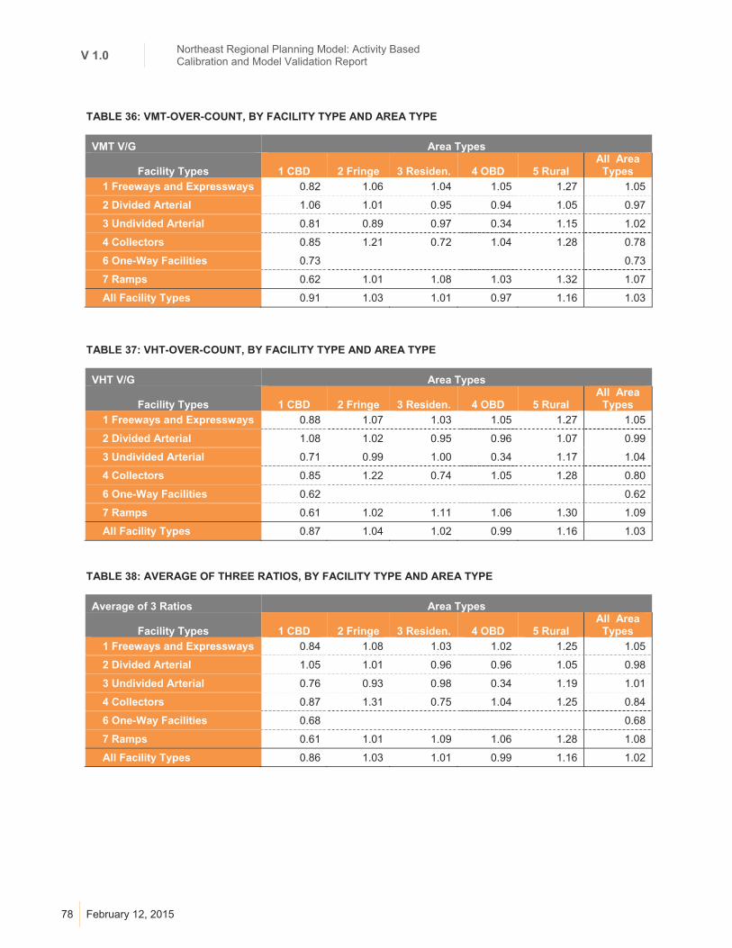
V 1.0 Northeast Regional Planning Model: Activity Based Calibration and Model Validation Report
78 February 12, 2015
TABLE 36: VMT-OVER-COUNT, BY FACILITY TYPE AND AREA TYPE
VMT V/G Area Types
Facility Types 1 CBD 2 Fringe 3 Residen. 4 OBD 5 Rural All Area
Types
1 Freeways and Expressways 0.82 1.06 1.04 1.05 1.27 1.05
2 Divided Arterial 1.06 1.01 0.95 0.94 1.05 0.97
3 Undivided Arterial 0.81 0.89 0.97 0.34 1.15 1.02
4 Collectors 0.85 1.21 0.72 1.04 1.28 0.78
6 One-Way Facilities 0.73 0.73
7 Ramps 0.62 1.01 1.08 1.03 1.32 1.07
All Facility Types 0.91 1.03 1.01 0.97 1.16 1.03
TABLE 37: VHT-OVER-COUNT, BY FACILITY TYPE AND AREA TYPE
VHT V/G Area Types
Facility Types 1 CBD 2 Fringe 3 Residen. 4 OBD 5 Rural All Area
Types
1 Freeways and Expressways 0.88 1.07 1.03 1.05 1.27 1.05
2 Divided Arterial 1.08 1.02 0.95 0.96 1.07 0.99
3 Undivided Arterial 0.71 0.99 1.00 0.34 1.17 1.04
4 Collectors 0.85 1.22 0.74 1.05 1.28 0.80
6 One-Way Facilities 0.62 0.62
7 Ramps 0.61 1.02 1.11 1.06 1.30 1.09
All Facility Types 0.87 1.04 1.02 0.99 1.16 1.03
TABLE 38: AVERAGE OF THREE RATIOS, BY FACILITY TYPE AND AREA TYPE
Average of 3 Ratios Area Types
Facility Types 1 CBD 2 Fringe 3 Residen. 4 OBD 5 Rural All Area
Types
1 Freeways and Expressways 0.84 1.08 1.03 1.02 1.25 1.05
2 Divided Arterial 1.05 1.01 0.96 0.96 1.05 0.98
3 Undivided Arterial 0.76 0.93 0.98 0.34 1.19 1.01
4 Collectors 0.87 1.31 0.75 1.04 1.25 0.84
6 One-Way Facilities 0.68 0.68
7 Ramps 0.61 1.01 1.09 1.06 1.28 1.08
All Facility Types 0.86 1.03 1.01 0.99 1.16 1.02

79
SCREENLINE, CUTLINE, AND CORDON COMPARISONS
NERPM model screenline, cutline and cordon locations are shown below in Figure 32 and Figure 33.6 Comparisons of 2010 AADT and modeled volumes at screenline, cutline, and cordon locations are shown below in Figure 34 and Table 39.
The right-most column of the table provides standards for the maximum percent deviation for daily counts from two different sources, the NCHRP 255 report7 and the FDOT validation standards manual8. The 2008 FSUTMS-Cube Framework Phase II standards are considerably more stringent than the NCHRP 255 standards, which were the benchmark values used to validate previous versions of NERPM.
As shown in Table 39, a majority (27 of 41) cutline and cordon locations meet the stricter FDOT standards, including important locations crossing the St. John’s River near downtown Jacksonville. Just six locations exceed the NCHRP 255 standards. The locations that deviate the most from the counts tend to be some of the more rural locations. None of the deviations is excessively large, but all are over-predicting rather than under-predicting. Only one location exceeds 50%, the relatively low-volume Cutline #27 (South Central Clay), which is over-predicted by 52%.
6 Source: The Corradino Group and PBS&J, Inc. (2009). Northeast Regional Planning Model 4.0: 2005 and 2035 Models, (Draft) Technical Report 1& 2, Model Data, Calibration and Validation, Pages 2-21 and 2-22. 7 Pedersen, N.J. and D.R. Samdahl (1982). National Cooperative Highway Research Program Report 255: Highway Traffic Data for Urbanized Area Project Planning and Design. Transportation Research Board, Page. 49. 8 FDOT (2008). FSUTMS-Cube Framework Phase II: Model Calibration and Validation Standards, Page 2-19.
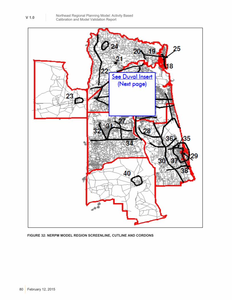
V 1.0 Northeast Regional Planning Model: Activity Based Calibration and Model Validation Report
80 February 12, 2015
FIGURE 32: NERPM MODEL REGION SCREENLINE, CUTLINE AND CORDONS

81
FIGURE 33: NERPM MODEL REGION SCREENLINE, CUTLINE AND CORDONS (DUVAL INSET)
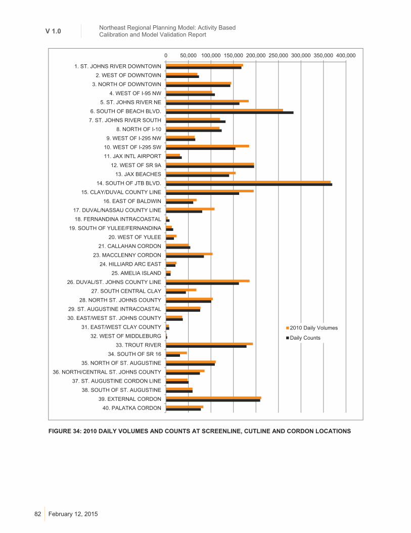
V 1.0 Northeast Regional Planning Model: Activity Based Calibration and Model Validation Report
82 February 12, 2015
FIGURE 34: 2010 DAILY VOLUMES AND COUNTS AT SCREENLINE, CUTLINE AND CORDON LOCATIONS
0 50,000 100,000 150,000 200,000 250,000 300,000 350,000 400,000
1. ST. JOHNS RIVER DOWNTOWN
2. WEST OF DOWNTOWN
3. NORTH OF DOWNTOWN
4. WEST OF I-95 NW
5. ST. JOHNS RIVER NE
6. SOUTH OF BEACH BLVD.
7. ST. JOHNS RIVER SOUTH
8. NORTH OF I-10
9. WEST OF I-295 NW
10. WEST OF I-295 SW
11. JAX INTL AIRPORT
12. WEST OF SR 9A
13. JAX BEACHES
14. SOUTH OF JTB BLVD.
15. CLAY/DUVAL COUNTY LINE
16. EAST OF BALDWIN
17. DUVAL/NASSAU COUNTY LINE
18. FERNANDINA INTRACOASTAL
19. SOUTH OF YULEE/FERNANDINA
20. WEST OF YULEE
21. CALLAHAN CORDON
23. MACCLENNY CORDON
24. HILLIARD ARC EAST
25. AMELIA ISLAND
26. DUVAL/ST. JOHNS COUNTY LINE
27. SOUTH CENTRAL CLAY
28. NORTH ST. JOHNS COUNTY
29. ST. AUGUSTINE INTRACOASTAL
30. EAST/WEST ST. JOHNS COUNTY
31. EAST/WEST CLAY COUNTY
32. WEST OF MIDDLEBURG
33. TROUT RIVER
34. SOUTH OF SR 16
35. NORTH OF ST. AUGUSTINE
36. NORTH/CENTRAL ST. JOHNS COUNTY
37. ST. AUGUSTINE CORDON LINE
38. SOUTH OF ST. AUGUSTINE
39. EXTERNAL CORDON
40. PALATKA CORDON
2010 Daily Volumes
Daily Counts

83
TABLE 39: 2010 DAILY VOLUME-COUNT DEVIATIONS, BY SCREENLINE, CUTLINE AND CORDON
No. Names 2010
AADT Daily
Volumes %
Deviation
NCHRP 255 Max. % Dev.*
FDOT Max. % Dev.**
1 St. Johns River Downtown (CL) 5 167,800 171,573 2.2% 19% 10%
2 West of Downtown (CL) 12 73,600 70,010 -4.9% 23% 10%
3 North of Downtown (CL) 6 143,100 145,370 1.6% 21% 10%
4 West of 1-95 NW (CL) 9 108,900 102,820 -5.6% 21% 10%
5 St. Johns River NE (CL) 6 163,402 183,986 12.6% 19% 10%
6 South of Beach Blvd. (SL) 20 283,500 260,197 -8.2% * 10%
7 St. Johns River South (CL) 3 132,500 120,284 -9.2% 22% 10%
8 North of 1-10 (CL) 13 124,000 119,103 -3.9% 22% 10%
9 West of 1-295 NW (CL) 10 65,300 63,999 -2.0% 25% 10%
10 West of 1-295 SW (CL) 10 154,500 184,968 19.7% 19% 10%
11 Jax lnt'l Airport (CL) 6 35,300 31,359 -11.2% 34% 15%
12 West of SR 9A (CL) 10 196,000 195,854 -0.1% 15% 10%
13 Jax Beaches (CL) 7 140,552 154,978 10.3% 20% 10%
14 South of JTB Blvd. (SL) 12 369,600 366,208 -0.9% * 10%
15 Clay/Duval County Line (SL) 8 162,700 195,113 19.9% 19% 10%
16 East of Baldwin (CL) 6 60,768 68,177 12.2% 31% 15%
17 Duval/Nassau County Line (SL) 8 80,760 108,176 33.9% 25% 10%
18 Fernandina Intracoastal (CL) 6 8,100 4,132 -49.0% 60% 20%
19 South of Yulee/Fernandina (CL) 4 16,200 13,165 -18.7% 53% 20%
20 West of Yulee (CL) 4 17,934 23,759 32.5% 50% 20%
21 Callahan Cordon (COR) 6 54,300 51,034 -6.0% 32% 15%
23 Macclenny Cordon, Baker County 84,500 103,766 22.8% 22% 10%
24 Hilliard Arc East (CUCOR) 7 21,200 23,520 10.9% 49% 20%
25 Amelia Island (CL) 2 10,500 10,942 4.2% 59% 20%
26 Duval/St. Johns County Line (CL) 6 162,272 185,940 14.6% 19% 10%
27 South Central Clay (CL) 7 44,468 67,746 52.3% 35% 15%
28 North St. Johns County (CUSL) 8 100,800 104,188 3.4% 23% 10%
29 St. Augustine Intracoastal (CL) 4 76,200 76,940 1.0% 28% 10%
30 East/West St. Johns County (CL) 9 37,600 36,400 -3.2% 29% 10%
31 East/West Clay County (CL) 7 7,400 6,821 -7.8% 53% 20%
32 West of Middleburg (CL) 3 2,900 2,201 -24.1% 65% 20%
33 Trout River (CL)_ 8 179,100 193,329 7.9% 17% 10%
34 South of SR 16 (CL) 5 31,300 46,797 49.5% 42% 20%
35 North of St. Augustine (CL) 7 108,700 110,821 2.0% 23% 10%
36 North/Central St. Johns Cnty (CL) 7 75,500 85,893 13.8% 26% 10%
37 St. Augustine Cordon Line (COR) 11 50,500 48,102 -4.7% 28% 10%
38 South of St. Augustine (CL) 6 59,300 59,220 -0.1% 32% 15%
39 External Cordon (SCUCOR) 35 209,422 211,858 1.2% 21% 1%
40 Palatka Cordon 77,700 83,280 7.2% 28% 10%
99 MISC. COUNTS (*) 15,938,847 15,936,495 0.0% * 5%
* NCHRP 255 guidelines graph showing “maximum desirable deviations” covers base-year counts less than 200,000.
** FDOT (2008). FSUTMS-Cube Framework Phase II: Model Calibration and Validation Standards, Page 2-19.
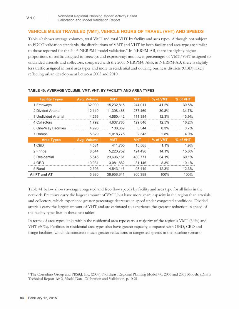
V 1.0 Northeast Regional Planning Model: Activity Based Calibration and Model Validation Report
84 February 12, 2015
VEHICLE MILES TRAVELED (VMT), VEHICLE HOURS OF TRAVEL (VHT) AND SPEEDS
Table 40 shows average volumes, total VMT and total VHT by facility and area types. Although not subject to FDOT validation standards, the distributions of VMT and VHT by both facility and area type are similar to those reported for the 2005 NERPM4 model validation.9 In NERPM-AB, there are slightly higher proportions of traffic assigned to freeways and expressways and lower percentages of VMT/VHT assigned to undivided arterials and collectors, compared with the 2005 NERPM4. Also, in NERPM-AB, there is slightly less traffic assigned in rural area types and more in residential and outlying business districts (OBD), likely reflecting urban development between 2005 and 2010.
TABLE 40: AVERAGE VOLUME, VMT, VHT, BY FACILITY AND AREA TYPES
Facility Types Avg. Volume VMT VHT % of VMT % of VHT
1 Freeways 32,999 15,232,815 244,011 41.2% 30.5%
2 Divided Arterial 12,149 11,398,466 277,469 30.8% 34.7%
3 Undivided Arterial 4,266 4,560,442 111,384 12.3% 13.9%
4 Collectors 1,792 4,637,783 129,846 12.5% 16.2%
6 One-Way Facilities 4,993 108,359 5,344 0.3% 0.7%
7 Ramps 5,329 1,018,775 2,343 2.8% 4.0%
Area Types Avg. Volume VMT VHT % of VMT % of VHT
1 CBD 4,531 411,700 15,565 1.1% 1.9%
2 Fringe 8,544 5,223,752 124,496 14.1% 15.6%
3 Residential 5,545 23,696,161 480,771 64.1% 60.1%
4 OBD 10,031 3,081,882 81,146 8.3% 10.1%
5 Rural 2,396 4,543,146 98,419 12.3% 12.3%
All FT and AT 5,930 36,956,641 800,398 100% 100%
Table 41 below shows average congested and free-flow speeds by facility and area type for all links in the network. Freeways carry the largest amount of VMT, but have more spare capacity in the region than arterials and collectors, which experience greater percentage decreases in speed under congested conditions. Divided arterials carry the largest amount of VHT and are estimated to experience the greatest reduction in speed of the facility types lists in these two tables.
In terms of area types, links within the residential area type carry a majority of the region’s VMT (64%) and VHT (60%). Facilities in residential area types also have greater capacity compared with OBD, CBD and fringe facilities, which demonstrate much greater reductions in congested speeds in the baseline scenario.
9 The Corradino Group and PBS&J, Inc. (2009). Northeast Regional Planning Model 4.0: 2005 and 2035 Models, (Draft) Technical Report 1& 2, Model Data, Calibration and Validation, p.10-21.

85
TABLE 41: AVERAGE FREEFLOW AND CONGESTED SPEEDS, BY FACILITY AND AREA TYPES
Facility Types Avg. Congested
Speed (mph) Avg. Freeflow Speed
(mph) % Change in Speed
1 Freeways 62.43 66.39 -6.0%
2 Divided Arterial 41.08 47.10 -12.8%
3 Undivided Arterial 40.94 44.58 -8.1%
4 Collectors 35.72 39.72 -10.1%
6 One-Way Facilities 20.28 21.19 -4.3%
7 Ramps 31.50 38.74 -18.7%
Area Types Avg. Congested
Speed (mph) Avg. Freeflow Speed
(mph) % Change in Speed
1 CBD 26.45 30.22 -12.5%
2 Fringe 41.96 48.17 -12.9%
3 Residential 49.29 53.66 -8.1%
4 OBD 37.98 47.00 -19.2%
5 Rural 46.16 49.00 -5.8%
All FT and AT 46.17 51.19 -9.8%
7.2 | AUXILIARY DEMAND
Daily EI/IE and EE trips tables were adjusted according to available counts at external stations, shown below in Table 42. The process started with the validated 2005 model EE and EI trip tables, which were factored to reflect the combined EE+EI trip ends at the external stations to make them equal to the 2010 counts at each location. The EE trip table was balanced to ensure symmetric flows.
Table 42 shows the assigned flows at each station, which are close to within +/-1% of at most of the count locations. The one noteworthy exception is at Station 2577 (I-95 South), which is off by -2%.
One reason for the difference from counts is the trip table creation process, whereby the daily EE and EI trips were allocated into vehicle classes and time periods, which resulted in some trips being gained or lost due to rounding. A second reason is that truck trips are generated and distributed by the regional truck model to reflect JAX Port (Jacksonville Port facilities) activities, the outcomes of which are not revealed until the truck trip distribution model is run. Many of these truck trips are destined to or originate at external stations. EI/IE trip table movements were adjusted to account for JAX Port trips based on a prior model run. JAX Port trips had the greatest effect on Stations 2550 and 2577 (I-95).

V 1.0 Northeast Regional Planning Model: Activity Based Calibration and Model Validation Report
86 February 12, 2015
TABLE 42: EXTERNAL STATION COUNTS AND MODELED VOLUMES
External Station ID Location
FDOT Daily 2-
Way Count
Model Daily 2-
Way Volume
Volume - Count
Percent Diff.
2550 I-95 North External 55,506 54,936 -570 -1.03%
2551 US 17 North External 3,400 3,396 -4 -0.13%
2552 US 1/SR 15 North External 8,896 8,893 -3 -0.03%
2553 CR 2 West External n/a 2,318 n/a 0.00%
2554 SR 121 North External 2,826 2,827 1 0.02%
2555 SR 2 North External-FL Grade 500 510 10 2.02%
2556 SR 2 West External n/a 811 n/a 0.00%
2557 CR 250 West External n/a 273 n/a 0.00%
2559 I-10 West External 20,476 20,368 -108 -0.53%
2560 US 90 West External 5,800 5,802 2 0.04%
2561 CR 231 South External n/a 299 n/a 0.00%
2563 SR 121 South External 3,700 3,702 2 0.05%
2564 US 301 South External 16,000 15,912 -88 -0.55%
2565 CR 225 West External 2,700 2,703 3 0.11%
2566 SR 16 West External 6,900 6,959 59 0.86%
2567 SR 230 West External 3,100 3,103 3 0.09%
2568 SR 100 North External 11,000 10,995 -5 -0.05%
2569 SR 26 West External 8,200 8,183 -17 -0.20%
2570 SR 20 West External 8,200 8,185 -15 -0.19%
2571 CR 21 South External n/a 798 n/a 0.00%
2572 CR 315 South External n/a 2,027 n/a 0.00%
2573 SR 19 South External 2,300 2,299 -1 -0.05%
2574 US 17 South External 4,500 4,496 -4 -0.08%
2575 SR 100 South External 3,500 3,499 -1 -0.03%
2576 US 1 South External 11,300 11,278 -22 -0.20%
2577 I-95 South External 45,500 44,465 -1,035 -2.28%
2578 SR A1A South External 4,000 3,997 -3 -0.07%
Totals for Stations with Counts 28,304 26,508 (1,796) -0.79%
7.3 | TRANSIT ASSIGNMENT
Figure 35 and Table 43 (below) show daily transit assignment results, by line. The total of assigned transit trips is 10% higher than boarding counts, which meets the FDOT acceptable and preferable validation standards for a regional planning model.
Individually most of the routes meet FDOT preferable validation standards, as shown in the right-most column of the table. The exceptions are routes SS50, TR1, TR3, WS52 and CT1, all of which are over-assigned. Of these, CT1 carries a large volume and may warrant further investigation. In addition, TR9 is vastly under-assigned, indicating a potential connectivity problem. A better fit to transit boardings would

87
require careful examination of walk-access connector links and/or adjustment to path-finding parameters as would be typical of a transit corridor study, an effort deemed to be beyond the scope of the LRTP.
FIGURE 35: TRANSIT LINE BOARDING COUNTS AND ASSIGNED VOLUMES
- 1,000 2,000 3,000 4,000 5,000 6,000
AR6
AR7
B7
B9
CT1
CT2
CT3
CT4
F1
K2
L7
L8
L9
M5
N6
NS19
P3
P4
R5
S1
SS 35
SS 50
SS6
SS8
TR 1
TR 3
TR10
TR9
U2
WS 2
WS12
WS52
WS6
WS7
X2
X4
Assigned Volumes
Daily Counts

V 1.0 Northeast Regional Planning Model: Activity Based Calibration and Model Validation Report
88 February 12, 2015
TABLE 43: TRANSIT LINE BOARDING COUNTS AND ASSIGNED VOLUMES
Route Name
Counts Assignment %
Difference FDOT
Acceptable FDOT
Preferable AR6 1,880 1,719 -9% +/-100% +/-65%
AR7 1,444 1,606 11% +/-100% +/-65%
B7 1,243 915 -26% +/-100% +/-65%
B9 756 1,275 69% +/-150% +/-100%
CT1 2,658 5,411 104% +/-65% +/-35%
CT2 1,047 577 -45% +/-100% +/-65%
CT3 1,009 238 -76% +/-100% +/-65%
CT4 2,789 2,621 -6% +/-65% +/-35%
F1 1,227 603 -51% +/-100% +/-65%
K2 2,501 3,050 22% +/-65% +/-35%
L7 2,368 3,050 29% +/-65% +/-35%
L8 2,606 3,698 42% +/-65% +/-35%
L9 947 713 -25% +/-150% +/-100%
M5 1,468 1,166 -21% +/-100% +/-65%
N6 769 818 6% +/-150% +/-100%
NS19 1,325 823 -38% +/-100% +/-65%
P3 743 751 1% +/-150% +/-100%
P4 2,071 2,286 10% +/-65% +/-35%
R5 1,201 917 -24% +/-100% +/-65%
S1 862 427 -50% +/-150% +/-100%
SS 35 70 124 77% +/-150% +/-100%
SS 50 21 97 362% +/-150% +/-100%
SS6 727 637 -12% +/-150% +/-100%
SS8 713 507 -29% +/-150% +/-100%
TR 1 406 1,658 308% +/-150% +/-100%
TR 3 495 1,476 198% +/-150% +/-100%
TR10 323 261 -19% +/-150% +/-100%
TR9 384 2 -99% +/-150% +/-100%
U2 705 657 -7% +/-150% +/-100%
WS 2 1,301 685 -47% +/-100% +/-65%
WS12 542 692 28% +/-150% +/-100%
WS52 78 253 224% +/-150% +/-100%
WS6 500 741 48% +/-150% +/-100%
WS7 747 445 -40% +/-150% +/-100%
X2 46 53 16% +/-150% +/-100%
X4 86 43 -50% +/-150% +/-100%
Total 24,005 26,030 8% +/-20% +/-10%
* FDOT (2008). FSUTMS-Cube Framework Phase II: Model Calibration and Validation Standards, Page 2-22.
89
8.0 COMPARATIVE EFFECTS OF 2010 AND 2040 DEMAND USING 2010 NETWORK
To test the behavior of NERPM-AB, the consultant team developed a scenario to test the impact of using 2040 socioeconomic data with the 2010 baseline network. The objective of this sensitivity tests was to look for logical behavioral responses under conditions in which the regional transportation system supply remains unchanged, while demand grows to fill the needs of an area population that is about 40% larger. This was not intended to be a realistic scenario, as it does not include any future investments infrastructure to support growth. Rather, it demonstrates that the activity-based demand portion of NERPM-AB responds appropriately to urban development, socioeconomic changes and the resulting congestion on the regional transportation system.
Of particular interest were changes to the following measures:
VMT and VHT Tour and trip rates Mean trip lengths Mode shares Highway volumes by facility and area type Time of day shifts Screenline, cutline and cordon volumes Transit boardings
The consultant team first developed TAZ-level control totals for 2040 households, employment, and school enrollment, an effort discussed in a separate technical memorandum (HNTB 2013).10 These TAZ-level data were used to create a 2040 marginal control totals from which a synthetic population was created using PopGen. The 2040 synthetic households, employment by industry group, and school enrollment totals by TAZ were subsequently allocated to the NERPM-AB land use parcel database. The entire model system was run with feedback to a convergent solution and key findings summarized.
Table 44, below, provides a summary of system-level changes between 2010 and 2040 scenarios. The total population for the region is estimated to grow by 41% and total employment by 39%. Consistent with demographic trends, average household size drops by 3% over this period. K-12 School enrollment is estimated to increase at a slightly higher rate, 44%, than the population, while university and college enrollment is expected to increase of just 20%.
The weekday VMT per household increases by a modest amount, 2%, while the VHT per household increases by 22%, indicating that households are traveling a little farther on average and doing so a little slower by spending much more time on the roadways. On a per person basis, this leads to VMT and VHT increase of 6% and 27%, respectively.
10 HNTB (2013). Path Forward 2040: Long Range Transportation Plan Draft Technical Memorandum #3, 2040 Socio Economic Data Forecasts.
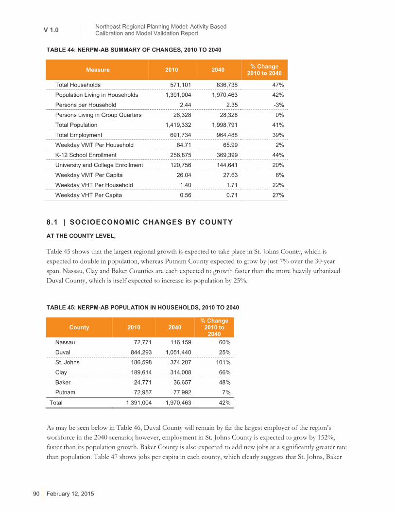
V 1.0 Northeast Regional Planning Model: Activity Based Calibration and Model Validation Report
90 February 12, 2015
TABLE 44: NERPM-AB SUMMARY OF CHANGES, 2010 TO 2040
Measure 2010 2040 % Change
2010 to 2040
Total Households 571,101 836,738 47%
Population Living in Households 1,391,004 1,970,463 42%
Persons per Household 2.44 2.35 -3%
Persons Living in Group Quarters 28,328 28,328 0%
Total Population 1,419,332 1,998,791 41%
Total Employment 691,734 964,488 39%
Weekday VMT Per Household 64.71 65.99 2%
K-12 School Enrollment 256,875 369,399 44%
University and College Enrollment 120,756 144,641 20%
Weekday VMT Per Capita 26.04 27.63 6%
Weekday VHT Per Household 1.40 1.71 22%
Weekday VHT Per Capita 0.56 0.71 27%
8.1 | SOCIOECONOMIC CHANGES BY COUNTY
AT THE COUNTY LEVEL,
Table 45 shows that the largest regional growth is expected to take place in St. Johns County, which is expected to double in population, whereas Putnam County expected to grow by just 7% over the 30-year span. Nassau, Clay and Baker Counties are each expected to growth faster than the more heavily urbanized Duval County, which is itself expected to increase its population by 25%.
TABLE 45: NERPM-AB POPULATION IN HOUSEHOLDS, 2010 TO 2040
County 2010 2040 % Change
2010 to 2040
Nassau 72,771 116,159 60%
Duval 844,293 1,051,440 25%
St. Johns 186,598 374,207 101%
Clay 189,614 314,008 66%
Baker 24,771 36,657 48%
Putnam 72,957 77,992 7%
Total 1,391,004 1,970,463 42%
As may be seen below in Table 46, Duval County will remain by far the largest employer of the region’s workforce in the 2040 scenario; however, employment in St. Johns County is expected to grow by 152%, faster than its population growth. Baker County is also expected to add new jobs at a significantly greater rate than population. Table 47 shows jobs per capita in each county, which clearly suggests that St. Johns, Baker

91
and, to a lesser extent, Putnam will become more mixed and less dependent on Duval County for jobs. In the case of St. Johns, it is expected to attract more workers from other counties. School enrollment figures by county, as shown in Table 48, are roughly proportional to population increases in each county. In contrast, college and university enrollment increases are spread somewhat uniformly across the five counties where campuses exist today, as shown in Table 49.
TABLE 46: NERPM-AB EMPLOYMENT, 2010 TO 2040
County 2010 2040 % Change
2010 to 2040
Nassau 24,126 39,586 64%
Duval 519,142 636,131 23%
St. Johns 61,714 155,427 152%
Clay 54,454 89,069 64%
Baker 7,396 13,860 87%
Putnam 25,148 30,415 21%
Total 691,980 964,488 39%
TABLE 47: NERPM-AB JOBS PER CAPITA, 2010 TO 2040
County 2010 2040 % Change
2010 to 2040
Nassau 0.33 0.34 3%
Duval 0.61 0.61 -2%
St. Johns 0.33 0.42 26%
Clay 0.29 0.28 -1%
Baker 0.30 0.38 27%
Putnam 0.34 0.39 13%
Total 0.50 0.49 -2%
TABLE 48: NERPM-AB K-12 SCHOOL ENROLLMENT, 2010 TO 2040
County 2010 2040 % Change
2010 to 2040
Nassau 12,101 18,973 57%
Duval 153,219 194,207 27%
St. Johns 33,647 73,468 118%
Clay 40,539 62,042 53%
Baker 5,228 7,613 46%
Putnam 12,141 13,096 8%
Total 256,875 369,399 44%
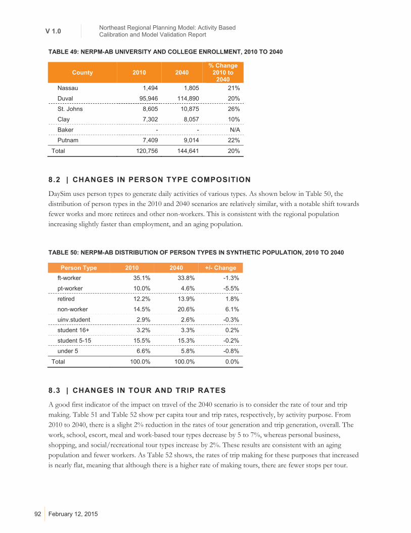
V 1.0 Northeast Regional Planning Model: Activity Based Calibration and Model Validation Report
92 February 12, 2015
TABLE 49: NERPM-AB UNIVERSITY AND COLLEGE ENROLLMENT, 2010 TO 2040
County 2010 2040 % Change
2010 to 2040
Nassau 1,494 1,805 21%
Duval 95,946 114,890 20%
St. Johns 8,605 10,875 26%
Clay 7,302 8,057 10%
Baker - - N/A
Putnam 7,409 9,014 22%
Total 120,756 144,641 20%
8.2 | CHANGES IN PERSON TYPE COMPOSITION
DaySim uses person types to generate daily activities of various types. As shown below in Table 50, the distribution of person types in the 2010 and 2040 scenarios are relatively similar, with a notable shift towards fewer works and more retirees and other non-workers. This is consistent with the regional population increasing slightly faster than employment, and an aging population.
TABLE 50: NERPM-AB DISTRIBUTION OF PERSON TYPES IN SYNTHETIC POPULATION, 2010 TO 2040
Person Type 2010 2040 +/- Change
ft-worker 35.1% 33.8% -1.3%
pt-worker 10.0% 4.6% -5.5%
retired 12.2% 13.9% 1.8%
non-worker 14.5% 20.6% 6.1%
uinv.student 2.9% 2.6% -0.3%
student 16+ 3.2% 3.3% 0.2%
student 5-15 15.5% 15.3% -0.2%
under 5 6.6% 5.8% -0.8%
Total 100.0% 100.0% 0.0%
8.3 | CHANGES IN TOUR AND TRIP RATES
A good first indicator of the impact on travel of the 2040 scenario is to consider the rate of tour and trip making. Table 51 and Table 52 show per capita tour and trip rates, respectively, by activity purpose. From 2010 to 2040, there is a slight 2% reduction in the rates of tour generation and trip generation, overall. The work, school, escort, meal and work-based tour types decrease by 5 to 7%, whereas personal business, shopping, and social/recreational tour types increase by 2%. These results are consistent with an aging population and fewer workers. As Table 52 shows, the rates of trip making for these purposes that increased is nearly flat, meaning that although there is a higher rate of making tours, there are fewer stops per tour.
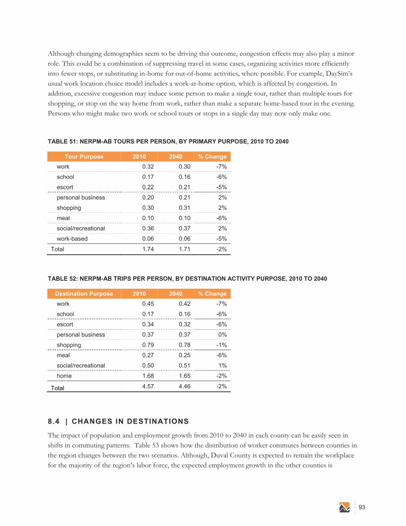
93
Although changing demographics seem to be driving this outcome, congestion effects may also play a minor role. This could be a combination of suppressing travel in some cases, organizing activities more efficiently into fewer stops, or substituting in-home for out-of-home activities, where possible. For example, DaySim’s usual work location choice model includes a work-at-home option, which is affected by congestion. In addition, excessive congestion may induce some person to make a single tour, rather than multiple tours for shopping, or stop on the way home from work, rather than make a separate home-based tour in the evening. Persons who might make two work or school tours or stops in a single day may now only make one.
TABLE 51: NERPM-AB TOURS PER PERSON, BY PRIMARY PURPOSE, 2010 TO 2040
Tour Purpose 2010 2040 % Change
work 0.32 0.30 -7%
school 0.17 0.16 -6%
escort 0.22 0.21 -5%
personal business 0.20 0.21 2%
shopping 0.30 0.31 2%
meal 0.10 0.10 -6%
social/recreational 0.36 0.37 2%
work-based 0.06 0.06 -5%
Total 1.74 1.71 -2%
TABLE 52: NERPM-AB TRIPS PER PERSON, BY DESTINATION ACTIVITY PURPOSE, 2010 TO 2040
Destination Purpose 2010 2040 % Change
work 0.45 0.42 -7%
school 0.17 0.16 -6%
escort 0.34 0.32 -6%
personal business 0.37 0.37 0%
shopping 0.79 0.78 -1%
meal 0.27 0.25 -6%
social/recreational 0.50 0.51 1%
home 1.68 1.65 -2%
Total 4.57 4.46 -2%
8.4 | CHANGES IN DESTINATIONS
The impact of population and employment growth from 2010 to 2040 in each county can be easily seen in shifts in commuting patterns. Table 53 shows how the distribution of worker commutes between counties in the region changes between the two scenarios. Although, Duval County is expected to remain the workplace for the majority of the region’s labor force, the expected employment growth in the other counties is
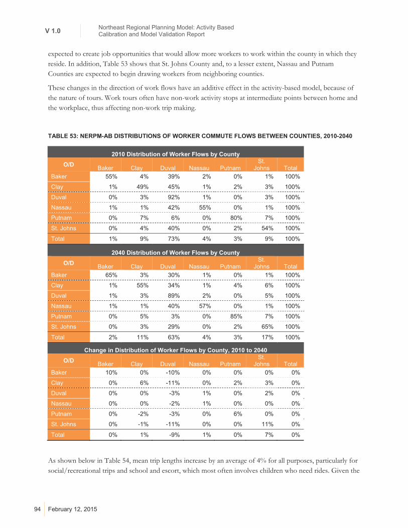
V 1.0 Northeast Regional Planning Model: Activity Based Calibration and Model Validation Report
94 February 12, 2015
expected to create job opportunities that would allow more workers to work within the county in which they reside. In addition, Table 53 shows that St. Johns County and, to a lesser extent, Nassau and Putnam Counties are expected to begin drawing workers from neighboring counties.
These changes in the direction of work flows have an additive effect in the activity-based model, because of the nature of tours. Work tours often have non-work activity stops at intermediate points between home and the workplace, thus affecting non-work trip making.
TABLE 53: NERPM-AB DISTRIBUTIONS OF WORKER COMMUTE FLOWS BETWEEN COUNTIES, 2010-2040
2010 Distribution of Worker Flows by County
O/D Baker Clay Duval Nassau Putnam
St. Johns Total
Baker 55% 4% 39% 2% 0% 1% 100%
Clay 1% 49% 45% 1% 2% 3% 100%
Duval 0% 3% 92% 1% 0% 3% 100%
Nassau 1% 1% 42% 55% 0% 1% 100%
Putnam 0% 7% 6% 0% 80% 7% 100%
St. Johns 0% 4% 40% 0% 2% 54% 100%
Total 1% 9% 73% 4% 3% 9% 100%
2040 Distribution of Worker Flows by County
O/D Baker Clay Duval Nassau Putnam
St. Johns Total
Baker 65% 3% 30% 1% 0% 1% 100%
Clay 1% 55% 34% 1% 4% 6% 100%
Duval 1% 3% 89% 2% 0% 5% 100%
Nassau 1% 1% 40% 57% 0% 1% 100%
Putnam 0% 5% 3% 0% 85% 7% 100%
St. Johns 0% 3% 29% 0% 2% 65% 100%
Total 2% 11% 63% 4% 3% 17% 100%
Change in Distribution of Worker Flows by County, 2010 to 2040
O/D Baker Clay Duval Nassau Putnam
St. Johns Total
Baker 10% 0% -10% 0% 0% 0% 0%
Clay 0% 6% -11% 0% 2% 3% 0%
Duval 0% 0% -3% 1% 0% 2% 0%
Nassau 0% 0% -2% 1% 0% 0% 0%
Putnam 0% -2% -3% 0% 6% 0% 0%
St. Johns 0% -1% -11% 0% 0% 11% 0%
Total 0% 1% -9% 1% 0% 7% 0%
As shown below in Table 54, mean trip lengths increase by an average of 4% for all purposes, particularly for social/recreational trips and school and escort, which most often involves children who need rides. Given the

95
anticipated higher growth in the less densely outer counties, compared with Duval County the increase in trip lengths is reasonable.
As shown in Table 55, mean trip durations increase by an average of 19% for all trip types, spread fairly uniformly across all purposes. That the increase in travel times is so much greater than the increase in trip lengths is due to network congestion effects. As stated above, there were no changes made to the 2010 highway or transit networks for the 2040 scenario; therefore, greater demand is being routed through the same supply, producing slower travel speeds.
TABLE 54: NERPM-AB MEAN TRIP DISTANCES IN MILES, BY DESTINATION ACTIVITY PURPOSE, 2010 TO 2040
Destination Purpose 2010 2040 % Change
work 10.02 10.29 3%
school 5.65 6.13 8%
escort 5.68 6.12 8%
personal business 6.93 7.08 2%
shopping 4.80 4.86 1%
meal 4.86 4.95 2%
social/recreational 5.24 5.87 12%
home 6.75 7.03 4%
TABLE 55: NERPM-AB MEAN TRIP DURATIONS IN MINUTES, BY DESTINATION ACTIVITY PURPOSE, 2010 TO 2040
Destination Purpose 2010 2040 % Change
work 14.10 15.93 13%
school 9.91 11.26 14%
escort 9.09 10.49 15%
personal business 11.18 13.26 19%
shopping 8.48 10.09 19%
meal 9.29 10.91 17%
social/recreational 12.30 14.94 21%
home 11.97 14.26 19%
8.5 | CHANGE IN MODE SHARES
As shown below in Table 56, despite a 40% increase in the number of tours, there was very little change in predicted mode shares, with one exception. The share of tours for which walking was the primary mode did increase significantly, taking a little bit of the market from the other modes, especially transit. Since no additional transit service is included in this 2040 scenario, persons living in households with fewer or no vehicles are more likely to choose nearer destinations and walk, compared with the 2010 scenario. This

V 1.0 Northeast Regional Planning Model: Activity Based Calibration and Model Validation Report
96 February 12, 2015
outcome is also made possible by increased employment in the outer counties. In the 2040 scenario, the proximity of new activity opportunities, such as shopping, restaurants, and services nearer to where residents live could make walking a more attractive option for some tours.
TABLE 56: NERPM-AB TOURS BY PRIMARY MODE, 2010 TO 2040
2010 2040
Tour Mode Tours Share Tours % Share Change in
Share
Drive Alone 848,955 36.43% 1,209,371 36.96% 0.5%
Shared Ride 2 599,373 25.72% 838,989 25.64% -0.1%
Shared Ride 3+ 548,315 23.53% 748,478 22.87% -0.7%
Park and Ride 472 0.02% 510 0.02% 0.0%
Kiss and Ride 961 0.04% 660 0.02% 0.0%
Walk-Transit 20,133 0.86% 20,894 0.64% -0.2%
Bike 42,771 1.84% 52,057 1.59% -0.2%
Walk 193,608 8.31% 296,795 9.07% 0.8%
School Bus 75,631 3.25% 104,506 3.19% -0.1%
Total 2,330,219 100.00% 3,272,260 100.00% 0.0%
8.6 | CHANGES IN HIGHWAY ASSIGNMENT OF BY FACILITY TYPE, AREA TYPE, TIME PERIOD AND COUNTY
Changes in assigned volumes are shown below in Table 57 and Table 58 for facility type and area type, respectively. Taken together, these tables suggest that undivided arterials would increase in volumes more than other facility types, and that rural, residential and CBD area types would be most affected. This likely to be consistent with the parts of the region that would experience the greatest growth in demand under the 2040 scenario.
TABLE 57: CHANGES IN HIGHWAY ASSIGNMENT VOLUMES BY FACILITY TYPE AND TIME PERIOD, 2010 TO 2040
Facility Type Daily AM Peak Midday
Off Peak PM Peak
Night Off Peak
1 Freeways & Exways 33% 28% 38% 26% 43% 2 Divided Arterial 36% 33% 36% 33% 40% 3 Undivided Arterial 55% 53% 55% 54% 58% 4 Collectors 32% 31% 37% 32% 40% 6 One-Way Facilities 31% 23% 30% 29% 29% 7 Ramps 28% 22% 31% 21% 34%
All Types 36% 32% 38% 32% 42%
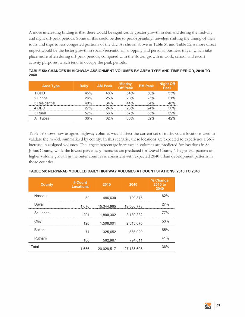
97
A more interesting finding is that there would be significantly greater growth in demand during the mid-day and night off-peak periods. Some of this could be due to peak-spreading, travelers shifting the timing of their tours and trips to less congested portions of the day. As shown above in Table 51 and Table 52, a more direct impact would be the faster growth in social/recreational, shopping and personal business travel, which take place more often during off-peak periods, compared with the slower growth in work, school and escort activity purposes, which tend to occupy the peak periods.
TABLE 58: CHANGES IN HIGHWAY ASSIGNMENT VOLUMES BY AREA TYPE AND TIME PERIOD, 2010 TO 2040
Area Type Daily AM Peak Midday
Off Peak PM Peak
Night Off Peak
1 CBD 45% 48% 54% 50% 53% 2 Fringe 26% 25% 28% 25% 31% 3 Residential 40% 34% 44% 34% 48% 4 OBD 27% 24% 28% 24% 30% 5 Rural 57% 56% 57% 55% 59%
All Types 36% 32% 38% 32% 42%
Table 59 shows how assigned highway volumes would affect the current set of traffic count locations used to validate the model, summarized by county. In this scenario, these locations are expected to experience a 36% increase in assigned volumes. The largest percentage increases in volumes are predicted for locations in St. Johns County, while the lowest percentage increases are predicted for Duval County. The general pattern of higher volume growth in the outer counties is consistent with expected 2040 urban development patterns in those counties.
TABLE 59: NERPM-AB MODELED DAILY HIGHWAY VOLUMES AT COUNT STATIONS, 2010 TO 2040
County # Count
Locations 2010 2040
% Change 2010 to
2040
Nassau
82
486,630
790,376 62%
Duval
1,076
15,344,965
19,560,778 27%
St. Johns
201
1,800,302
3,189,332 77%
Clay
126
1,508,001
2,313,670 53%
Baker
71
325,652
536,929 65%
Putnam
100
562,967
794,611 41%
Total
1,656
20,028,517
27,185,695 36%

V 1.0 Northeast Regional Planning Model: Activity Based Calibration and Model Validation Report
98 February 12, 2015
8.7 | SCREENLINE, CUTLINE AND CORDON VOLUMES
Changes to screenline, cutline and cordon volumes are shown below in Figure 36. Across the region, these volumes exhibit remarkably proportional growth. Locations that carried larger volumes in 2010 seem to grow proportionally in 2040. In the 2040 scenario, the fastest growing county is expected to be St. Johns. The chart show larger gains at locations that capture flows between St. John’s County and Duval County to the north: Locations 14 (JTB Boulevard), 26 (Duval/St. Johns County Line), 28 (North St. Johns), and 35 (St. Augustine cordon). In addition, Location 33 (Trout River), just to the north of Downtown Jacksonville, and Location 17 (Duval-Nassau County Line) show proportionally higher growth, suggesting greater traffic growth in the I-95 corridor towards Nassau County. External station cordons are also expected to grow at a high rate, although this growth is driven by projections applied to external trip tables, not by the activity-based demand model.

99
FIGURE 36: CHANGES IN MODEL VOLUMES , 2010 TO 2040, AT SCREENLINE, CUTLINE AND CORDON LOCATIONS
0 50,000 100,000150,000200,000250,000300,000350,000400,000450,000
1. ST. JOHNS RIVER DOWNTOWN
2. WEST OF DOWNTOWN
3. NORTH OF DOWNTOWN
4. WEST OF I-95 NW
5. ST. JOHNS RIVER NE
6. SOUTH OF BEACH BLVD.
7. ST. JOHNS RIVER SOUTH
8. NORTH OF I-10
9. WEST OF I-295 NW
10. WEST OF I-295 SW
11. JAX INTL AIRPORT
12. WEST OF SR 9A
13. JAX BEACHES
14. SOUTH OF JTB BLVD.
15. CLAY/DUVAL COUNTY LINE
16. EAST OF BALDWIN
17. DUVAL/NASSAU COUNTY LINE
18. FERNANDINA INTRACOASTAL
19. SOUTH OF YULEE/FERNANDINA
20. WEST OF YULEE
21. CALLAHAN CORDON
23. MACCLENNY CORDON
24. HILLIARD ARC EAST
25. AMELIA ISLAND
26. DUVAL/ST. JOHNS COUNTY LINE
27. SOUTH CENTRAL CLAY
28. NORTH ST. JOHNS COUNTY
29. ST. AUGUSTINE INTRACOASTAL
30. EAST/WEST ST. JOHNS COUNTY
31. EAST/WEST CLAY COUNTY
32. WEST OF MIDDLEBURG
33. TROUT RIVER
34. SOUTH OF SR 16
35. NORTH OF ST. AUGUSTINE
36. NORTH/CENTRAL ST. JOHNS COUNTY
37. ST. AUGUSTINE CORDON LINE
38. SOUTH OF ST. AUGUSTINE
39. EXTERNAL CORDON
40. PALATKA CORDON
2010 Daily Volumes
2040 Daily Volumes

V 1.0 Northeast Regional Planning Model: Activity Based Calibration and Model Validation Report
100 February 12, 2015
8.8 | TRANSIT ASSIGNMENT
The 2040 scenario added no additional transit capacity or service. As discussed, transit mode shares were essentially unchanged, thus the results shown below in Figure 37 are expected. There are slight increases and decreases in assigned boardings, but there is little change, indicating stability in the assignment process.
FIGURE 37: CHANGES IN DAILY TRANSIT ASSIGNED BOARDINGS, 2010 TO 2040, BY LINE
- 1,000 2,000 3,000 4,000 5,000 6,000
AR6
AR7
B7
B9
CT1
CT2
CT3
CT4
F1
K2
L7
L8
L9
M5
N6
NS19
P3
P4
R5
S1
SS 35
SS 50
SS6
SS8
TR 1
TR 3
TR10
TR9
U2
WS 2
WS12
WS52
WS6
WS7
X2
X4
2010 Assignment
2040 Assignment