1

2

SYLLABUS

UNIT-I

Introduction, Nature of RADAR, Maximum Unambiguous range, Radar Waveforms, Block

schematics of pulse radar and Operation, simple form of radar equation, RADAR frequencies,

Applications of RADARS. Related problems.

UNIT-II

Radar Equation: Prediction of Range Performance, Minimum Detectable Signal, Receiver

Noise and SNR, Integration of Radar Pulses, Radar Cross Section of Targets (simple Targets-

sphere,cone-sphere),Transmitter Power, PRF and Range Ambiguities, System Losses(qualitative

treatment),Related Problems .

UNIT-III

CW and Frequency Modulated Radar: Doppler Effect, CW Radar – Block Diagram, Isolation

between Transmitter and Receiver, Non-zero IF Receiver, Receiver bandwidth requirements,

Applications of CW radar.

UNIT-IV

FM-CW Radar, Range and Doppler measurement, Block Diagram and Characteristics

(Approaching/Receding targets), FM-CW Altimeter, Measurement errors, Multiple Frequency

CWRadar

UNIT-V

MTI and Pulse Doppler radar: Introduction, Principle, MTI Radar with - Power Amplifier

Transmitter and Power Oscillator Transmitter, Delay Line Cancellers – Filter Characteristics,

Blind Speeds, Double Cancellation, Staggered PRFs. Range Gated Doppler Filters. MTI Radar

Parameters, Limitations to MTI Performance, Non-coherent MTI, MTI versus Pulse Doppler

Radar

3

UNIT-VI

Tracking Radar: Tracking with Radar, Sequential Lobing, Conical Scan, Monopulse Radar –

Amplitude Comparison and Phase Comparison Monopulse. Low angle tracking, tracking in

range,acquisition,ComparisonofTrackers.

UNIT-VII

Detection of Radar Signals in Noise: Introduction, Matched filter receiver-Response

Characteristics and Derivation, Correlation Function and Cross-Correlation receiver, Efficiency

of Non-matched Filters, matched Filter with Non-white Noise.

UNIT-VIII

Radar Receivers: Noise Figure and Noise temperature, Displays-types, Duplexers-Branch type

and Balanced type, Circulators as Duplexers. Introduction to Phased Array Antennas-Basic

Concepts, Radiation Pattern, Beam Steering and Beam Width Changes, Series versus Parallel

Feeds, Applications, Advantages and Limitations.

4

UNIT-I

NATURE OF

RADAR

5

INTRODUCTION:

The name Radar stands for Radio Detection and Ranging

Radar is a remote sensing technique: Capable of gathering information about objects located at

remote distances from the sensing device.

Two distinguishing characteristics:

1. Employs EM waves that fall into the microwave portion of the electromagnetic spectrum

(1 mm < l < 75 cm)

2. Active technique: radiation is emitted by radar – radiation scattered by objects is detected

by radar.

6

Radar is an electromagnetic system for the detection and location of objects

(Radio Detection and Ranging). Radar operates by transmitting a particular type of waveform

and detecting the nature of the signals reflected back from objects.

Radar can not resolve detail or color as well as the human eye (an optical frequency

passive scatter meter).

Radar can see in conditions which do not permit the eye to see such as darkness, haze,

rain, smoke.

Radar can also measure the distances to objects. The elemental radar system consists of a

transmitter unit, an antenna for emitting electromagnetic radiation and receiving the echo, an

energy detecting receiver and a processor.

Receiver

Transmitter

Range

Velocity

Position

Type etc.,

Range

A portion of the transmitted signal is intercepted by a reflecting object (target) and is

reradiated in all directions. The antenna collects the returned energy in the backscatter direction

and delivers it to the receiver. The distance to the receiver is determined by measuring the time

taken for the electromagnetic signal to travel to the target and back. The direction of the target is

determined by the angle of arrival (AOA) of the reflected signal. Also if there is relative motion

between the radar and the target, there is a shift in frequency of the reflected signal (Doppler

7

Effect) which is a measure of the radial component of the relative velocity. This can be used to

distinguish between moving targets and stationary ones.

Radar was first developed to warn of the approach of hostile aircraft and for directing anti

aircraft weapons. Modern radars can provide AOA, Doppler, and MTI etc.

RADAR RANGE MEASUREMENT

Target

• Target range = ct

2

where c = speed of light

t = round trip time

8

The simplest radar waveform is a train of narrow (0.1μs to 10μs) rectangular pulses

modulating a sinusoidal carrier the distance to the target is determined from the time TR taken by

the pulse to travel to the target and return and from the knowledge that electromagnetic energy

travels at the speed of light.

Since radio waves travel at the speed of light (v = c = 300,000 km/sec)

Range = c×time/2

The range or distance, R = cTR/2

R (in km) = 0.15TR (μs) R (in nmi) = 0.081TR (μs)

NOTE:

1 nmi = 6076 feet =1852 meters.

1 Radar mile = 2000 yards = 6000 feet

Radar mile is commonly used unit of distance.

NOTE:

Electromagnetic energy travels through air at approximately the speed of light:-

1. 300,000 kilometers per second.

2. 186,000 statute miles per second.

3. 162,000 nautical miles per second.

Once the pulse is transmitted by the radar a sufficient length of time must elapse before

the next pulse to allow echoes from targets at the maximum range to be detected. Thus the

maximum rate at which pulses can be transmitted is determined by the maximum range at which

targets are expected. This rate is called the pulse repetition rate (PRF).

If the PRF is too high echo signals from some targets may arrive after the transmission of

the next pulse. This leads to ambiguous range measurements. Such pulses are called second time

around pulses.

The range beyond which second time around pulses occur is called the maximum

unambiguous range.

9

RUNAMBIG = c/2f P Where fP is the PRF in Hz.

More advanced signal waveforms then the above are often used, for example the carrier

maybe frequency modulated (FM or chirp) or phase modulated (pseudorandom bi phase) too

permit the echo signals to be compressed in time after reception. This achieves high range

resolution without the need for short pulses and hence allows the use of the higher energy of

longer pulses. This technique is called pulse compression. Also CW waveforms can be used by

taking advantage of the Doppler shift to separate the received echo from the transmitted signal.

Note: unmodulated CW waveforms do not permit the measurement of range.

What is done by Radar?

Radar can see the objects in

day or night

rain or shine

land or air

cloud or clutter

fog or frost

earth or planets

stationary or moving and

Good or bad weather.

In brief, Radar can see the objects hidden any where in the globe or planets except hidden behind

good conductors.

INFORMATION GIVEN BY THE RADAR:

Radar gives the following information:

The position of the object

The distance of objects from the location of radar

10

The size of the object

Whether the object is stationary or moving

Velocity of the object

Distinguish friendly and enemy aircrafts

The images of scenes at long range in good and adverse weather conditions

Target recognition

Weather target is moving towards the radar or moving away

The direction of movement of targets

Classification of materials

NATURE AND TYPES OF RADARS:

The common types of radars are:

Speed trap Radars

Missile traking Radars

Early warning Radars

Airport control Radars

Navigation Radars

Ground mapping Radars

Astronomy Radars

Weather forecast Radars

Gun fire control Radars

Remote sensing Radars

Tracking Radars

Search Rdars

IFF (Identification Friend or Foe)

Synthetic apearture Radars

Missile control Radars

MTI (Moving Target Indication) Radars

Navy Radars

Doppler Radars

11

Mesosphere, Stratosphere and Troposphere (MST) Radars

Over-The-Horizon (OTH) Radars

Monopulse Radars

Phased array Radars

Instrumentation Radars

Gun direction Radars

Airborne weather Radars

12

PULSE CHARACTERISTICS OF RADAR SYSTEMS:

There are different pulse characteristics and factors that govern them in a Radar system

Carrier

Pulse width

Pulse Repetition Frequency(PRF)

Unambiguous Range

NOTE: ECHO is a reflected EM wave from a target and it is received by a Radar receiver.

CARRIER: The carrier is used in a Radar system is an RF(radio frequency) signal with

microwave frequencies.

Carrier is usually modulated to allow the system to capture the required data.

In simple ranging Radars, the carrier will be pulse modulated but in continuous wave systems

such Doppler radar modulation is not required.

In pulse modulation, the carrier is simply switched ON & OFF in synchronization.

PULSE WIDTH: The pulse width of the transmitted signal determines the dead zone. When the

Radar transmitter is active, the receiver input is blanked to avoid the damage of amplifiers. For

example, a Radar echo will take approximately 10.8 µsec to return from 1 standard mile away

target.

PULSE REPETITION FREQUENCY (PRF): PRF is the number of pulses transmitted per

second. PRF is equal to the reciprocal of pulse repetition time (PRT). It is measured in Hertz

PRF = 1/PRT

Pulse Interval Time or Pulse Reset Time (PRT) is the time interval between two pulses. It is

expressed in milliseconds.

Pulse Reset Time = Pulse Repetition Time – Pulse Width

UNAMBIGUOUS RANGE: In simple systems, echoes from targets must be detected and

processed before the next transmitter pulse is generated if range ambiguity is to be avoided.

13

Range ambiguity occurs when the time taken for an echo to return from a target is greater than

the pulse repetition period (T).

Echoes that arrive after the transmission of the next pulse are called as second-time-around

echoes.

The range beyond which targets appear as second-time-around echoes is called as the Maximum

Unambiguous Range and is given by

RUNAMBIG = c/2fP

c = velocity of propagation Where, TP = fP

fP is the PRF(PULSE REPETITION FREQUENCY) in Hz

TYPES OF BASIC RADARS:

Monostatic and Bistatic

CW

FM-CW

Pulsed radar

14

Monostatic radar uses the same antenna for transmit and receive. Its typical geometry is shown in

the below fig.

Bistatic radars use transmitting and receiving antennas placed in different locations.

CW radars, in which the two antennas are used, are not considered to be bistatic radars as the

distance between the antennas is not considerable. The bistatic radar geometry is shown in below

fig.

15

RADAR WAVE FORMS:

The most common Radar waveform is a train of narrow, rectangular shape pulses modulating a

sine-wave carrier.

The figure shows a pulse waveform, which can be utilized by the typical Radar.

16

From the given Radar waveform:

Peak power pt = 1 Mwatt

Pulse Width τ = 1 µsec.

Pulse Repetition Period TP = 1 msec.

A maximum unambiguous range of 150 km was provided by the PRF fP = 1000 Hz.

RUNAMBIG = c/2fP ==> 150×103 = 3×10

8 / 2fP

==> fP = 1000 Hz.

Then, the average power Pavg of a repetitive pulse train wave form is given by Pavg = pt τ/TP ==>

Pavg = pt τ fP

In this case, Pavg = 1 Kwatt

For a Radar wave form, the ratio of the total time that the Radar is radiating to the total time it

could have radiated is known as duty cycle.

Duty Cycle = τ/TP = τ fP = Pavg /pt

Duty Cycle = τ/TP = 0.001

The energy of the pulse is given by, E = τ pt = 1 Joule.

The Radar waveform can be extended in space over a distance of 300 meters using a pulse width

of 1 µsec.

i.e., Distance = c τ = 300 m.

Half of the above distance (i.e. c τ/2) can be used to recognize the two equal targets which

are being resolved in range. In this case, a separation of 150m between two equal size targets can

be used to resolve them.

17

Name Symbol Units Typical values

Transmitted

Frequencyft MHz, G hz 1000-12500 Mhz

Wavelength l cm 3-10 cm

Pulse Duration t M sec 1 m sec

Pulse Length h m 150-300 m (h=ct)

Pulse Repetition

FrequencyPRF sec-1 1000 sec-1

Interpulse Period T Milli sec 1 milli sec

Peak Transmitted

PowerPt MW 1 MW

Average Power Pavg kW 1 kW (Pavg = Pt t PRF)

Received Power Pr mW 10-6 mW

The Radar Range Equation:

The radar range equation relates the range of the radar to the characteristics of the

transmitter, receiver, antenna, target and the environment.

It is used as a tool to help in specifying radar subsystem specifications in the design phase

of a program. If the transmitter delivers PT Watts into an isotropic antenna, then the power

density (w/m2) at a distance R from the radar is

Pt/4πR2

Here the 4πR2 represents the surface area of the sphere at distance R

Radars employ directional antennas to channel the radiated power Pt in a particular

direction. The gain G of an antenna is the measure of the increased power radiated in the

direction of the target, compared to the power that would have been radiated from an isotropic

antenna

18

∴ Power density from a directional antenna = PtG/4πR2

The target intercepts a portion of the incident power and redirects it in various directions.

The measure of the amount of incident power by the target and redirected back in the direction of

the radar is called the cross section σ.

Hence the Power density of the echo signals at the radar =

Note: the radar cross-section σ has the units of area. It can be thought of as the size of the target

as seen by the radar.

The receiving antenna effectively intercepts the power of the echo signal at the radar over

a certain area called the effective area Ae.

Since the power density (Watts/m2) is intercepted across an area Ae, the power delivered

to the receiver is

Pr = (PtGσAe) /(4πR2)2

==> R4 = (PtGσAe) /(4π)

2 Pr

R = [(PtGσAe) /(4π)2 Pr]

1/4

Now the maximum range Rmax is the distance beyond which the target cannot be detected

due to insufficient received power Pr, the minimum power which the receiver can detect is called

the minimum detectable signal Smin. Setting, Pr = Smin and rearranging the above equation gives

Note here that we have both the antenna gain on transmit and its effective area on receive. These

are related by:

As long as the radar uses the same antenna for transmission and reception we have

19

Example: Use the radar range equation to determine the required transmit power for the TRACS

radar given: Prmin =10-13

Watts, G=2000, λ=0.23m, PRF=524, σ=2.0 m2

Now,

From

= 3.1 MW

Note 1: these three forms of the equation for Rmax varywith different powers of λ. This results

from implicit assumptions about the independence of G or Ae from λ.

Note 2: the introduction of additional constraints (such as the requirement to scan a specific

volume of space in a given time) can yield other λ dependence.

Note 3: The observed maximum range is often much smaller than that predicted from the above

equation due to the exclusion of factors such as rainfall attenuation, clutter, noise figure etc.

RADAR BLOCK DIAGRAM AND OPERATION:

The Transmitter may be an oscillator (magnetron) that is pulsed on and off bya modulator to

generate the pulse train.

the magnetron is the most widely used oscillator

typical power required to detect a target at 200 NM is MW peak power and several kW

average power

typical pulse lengths are several μs

typical PRFs are several hundreds of pulses per second

20

The waveform travels to the antenna where it is radiated. The receiver must be protected

from damage resulting from the high power of the transmitter. This is done by the duplexer.

duplexer also channels the return echo signals to the receiver and not to the transmitter

duplexer consists of 2 gas discharge tubes called the TR (transmit/receive) and the and an

ATR (anti transmit/receive) cell

The TR protects the receiver during transmission and the ATR directs the echo to the

receiver during reception.

solid state ferrite circulators and receiver protectors with gas plasma (radioactive keep

alive) tubes are also used in duplexers

The receiver is usually a superheterodyne type. The LNA is not always desirable. Although it

provides better sensitivity, it reduces the dy namic range of operation of the mix er. A receiver

with just a mixer front end has greater dynamic range, is less susceptible to overload and is less

vulnerable to electronic interference.

The mixer and Local Oscillator (LO) convert the RF frequency to the IF frequency.

The IF is typically 300MHz, 140Mz, 60 MHz, 30 MHz with bandwidths of 1 MHz to 10

MHz.

21

The IF strip should be designed to give a matched filter output. This requires its H(f) to

maximize the signal to noise power ratio at the output.

This occurs if the |H(f)| (magnitude of the frequency response of the IF strip is equal to

the signal spectrum of the echo signal |S(f)|, and the ARG(H(f)) (phase of the frequency

response) is the negative of the ARG(S(f)).

i.e. H(f) and S(f) should be complex conjugates

For radar with rectangular pulses, a conventional IF filter characteristic approximates a

matched filter if its bandwidth B and the pulse width τ satisfy the relationship

22

The pulse modulation is extracted by the second detector and amplified by video amplifiers

to levels at which they can be displayed (or A to D’d to a digital processor). The display is

usually a CRT; timing signals are applied to the display to provide zero range information. Angle

information is supplied from the pointing direction of the antenna.

The most common type of CRT display is the plan position indicator (PPI) which maps

the location of the target in azimuth and range in polar coordinates

The PPI is intensitymodulated bythe amplitude of the receiver output and the CRT

electron beam sweeps outward from the centre corresponding to range.

Also the beam rotates in angle in synchronization with the antenna pointing angle.

A B scope display uses rectangular coordinates to display range vs angle i.e. the x axis is

angle and the y axis is range.

Since both the PPI and B scopes use intensity modulation the dynamic range is limited

An A scope plots target echo amplitude vs range on rectangular coordinates for some

fixed direction. It is used primarily for tracking radar applications than for surveillance

radar.

The simple diagram has left out many details such as

AFC to compensate the receiver automatically for changes in the transmitter

AGC

Circuits in the receiver to reduce interference from other radars

Rotary joints in the transmission lines to allow for movement of the antenna

MTI (moving target indicator) circuits to discriminate between moving targets and

unwanted stationary targets

Pulse compression to achieve the resolution benefits of a short pulse but with the energy

benefits of a long pulse.

Monopulse tracking circuits for sensing the angular location of a moving target and

allowing the antenna to lock on and track the target automatically

Monitoring devices to monitor transmitter pulse shape, power load and receiver

sensitivity

23

Built in test equipment (BITE) for locating equipment failures so that faulty circuits can

be replaced quickly

Instead of displaying the raw video output directly on the CRT, it might be digitized and

processed and then displayed. This consists of:

Quantizing the echo level at range-azimuth resolution cells

Adding (integrating) the echo level in each cell

Establishing a threshold level that permits only the strong outputs due to target echoes to

pass while rejecting noise

Maintaining the tracks (trajectories) of each target

Displaying the processed information

This process is called automatic tracking and detection (ATD) in surveillance radar

Antennas:

The most common form of radar antenna is a reflector with parabolic shape, fed from a

point source (horn) at its focus

The beam is scanned in space by mechanically pointing the antenna

Phased array antennas are sometimes used. Her the beam is scanned by varying the phase

of the array elements electrically

Radar Frequencies:

Most Radar operates between 220 MHz and 35 GHz.

Special purpose radars operate out side of this range.

Skywave HF-OTH (over the horizon) can operate as low as 4 MHz

Groundwave HF radars operate as low as 2 MHz

Millimeter radars operate up to 95 GHz

Laser radars (lidars) operate in IR and visible spectrum

24

The radar frequencyletter -band nomenclature is shown in the table. Note that the

frequencyassignment to the latter band radar (e.g. L band radar) is much smaller than the

complete range of frequencies assigned to the letter band

25

Applications of Radar

General

i. Ground-based radar is applied chiefly to the detection, location and tracking of aircraft of

space targets

ii. Shipborne radar is used as a navigation aid and safety device to locate buoys, shorelines

and other ships. It is also used to observe aircraft

iii. Airborne radar is used to detect other aircraft, ships and land vehicles. It is also used for

mapping of terrain and avoidance of thunderstorms and terrain.

iv. Spaceborne radar is used for the remote sensing of terrain and sea, and for

rendezvous/docking.

26

Major Applications

1. Air Traffic Control

Used to provide air traffic controllers with position and other information on

aircraft flying within their area of responsibility (airways and in the vicinity of

airports)

High resolution radar is used at large airports to monitor aircraft and ground

vehicles on the runways, taxiways and ramps.

GCA (ground controlled approach) or PAR (precision approach radar) provides

an operator with high accuracy aircraft position information in both the vertical

and horizontal. The operator uses this information to guide the aircraft to a

landing in bad weather.

MLS (microwave landing system) and ATC radar beacon systems are based on

radar technology

2. Air Navigation

Weather avoidance radar is used on aircraft to detect and display areas of heavy

precipitation and turbulence.

Terrain avoidance and terrain following radar (primarily military)

Radio altimeter (FM/CW or pulse)

Doppler navigator

Ground mapping radar of moderate resolution sometimes used for navigation

3. Ship Safety

These are one of the least expensive, most reliable and largest applications of

radar

Detecting other craft and buoys to avoid collision

Automatic detection and tracking equipment (also called plot extractors) are

available with these radars for collision avoidance

Shore based radars of moderate resolution are used from harbour surveillance and

as an aid to navigation

4. Space

Radars are used for rendezvous and docking and was used for landing on the

moon

27

Large ground based radars are used for detection and tracking of satellites

Satellite-borne radars are used for remote sensing (SAR, synthetic aperture radar)

5. Remote Sensing

Used for sensing geophysical objects (the environment)

Radar astronomy - to probe the moon and planets

Ionospheric sounder (used to determine the best frequency to use for HF

communications)

Earth resources monitoring radars measure and map sea conditions, water resources,

ice cover, agricultural land use, forest conditions, geological formations,

environmental pollution (Synthetic Aperture Radar, SAR and Side Looking Airborne

Radar SLAR)

6. Law Enforcement

Automobile speed radars

Intrusion alarm systems

7. Military

Surveillance

Navigation , Fire control and guidance of weapons

ADVANTAGES OF BASIC RADAR:

It acts as a powerful eye.

It can see through: fog, rain, snow, darkness, haze, clouds and any insulators.

It can find out the range, angular position, location and velocity of targets.

LIMITATIONS:

Radar can not recognize the color of the targets.

It can not resolve the targets at short distances like human eye.

It can not see targets placed behind the conducting sheets.

It can not see targets hidden in water at long ranges.

28

It is difficult to identify short range objects.

The duplexer in radar provides switching between the transmitter and receiver

alternatively when a common antenna is used for transmission and reception.

The switching time of duplexer is critical in the operation of radar and it affects the

minimum range. A reflected pulse is not received during

the transmit pulse

subsequent receiver recovery time

The reflected pulses from close targets are not detected as they return before the receiver

is connected to the antenna by the duplexer.

Other Forms of the Radar Equation:-

FIRST EQUATION:-

If the transmit and receive antennas are not the same and have

different gains, the radar equation will

where Gt is the gain of transmit antenna and Gr is the gain of receive antenna .

SECOND EQUATION:-

If the target ranges are different for transmit and

receive antennas. The equation will be :

. Where Rt

and Rr are ranges between the target and the transmit antenna and the target and the

receive antenna respectively .

THIRD EQUATION:-

The first radar equation we discussed was derived without incorporating

losses of energy which accompany transmission, reception, and the processing of

electromagnetic radiation. It is sufficient to incorporate all of these losses in one term and

write equation as follows :- Where L is the total loss term.

29

FOURTH EQUATION:-

If we know that the signal power equals the noise

power S/N = 1 the equation will be :

.Note that

all of

The terms appearing in the Ro equation, with the exception of the target cross section, are a

characteristic of the radar system.

Once a design is established, Ro can be determined for a given target

size. Using the value of Ro

from the fourth

equation in the

third equation

we get

. From this equation, it is noted that S/N is inversely

proportional to the fourth power of

Range, R.

Parameters Affecting the Radar Range Equation:-

The radar equation was derived in the previous section and is below for reference:-

The terms of this equation, which depend on the:-

1) Physical structure of antenna. 2) Radar transmitter.

3) Processing of received signal. 4) System losses.

5) Characteristics of the target.

Type of Transmission:-

Passive: - there is no transmission.

Active: - there is transmission.

30

RADAR PARAMETERS AND DEFINITIONS:

RADAR: Radio means Radio Detection and Ranging. It is a device useful for detecting and

ranging, tracking and searching. It is useful for remote sensing, weather forecasting, speed

traping, fire control and astronomical abbrivations.

Echo: Echo is a reflected electromagnetic wave from a target and it is received by radar

receiver. The echo signal power is captured by the effective area of the receiving space antenna.

Duplexer: It is a microwave switch which connects the transmitter and receiver to the antenna

alternatively. It protects the receiver from high power output of the transmitter. It allows the use

of the single antenna for both radar transmistion and reception. It balnks the receiver during the

transmitting period.

Antenna: It is a device which acts as atransducer between transmitter and free space and

between free space and receiver. It converts electromagnetic energy into electrical energy at

receiving side and converts the electrical energy into electromagnetic energy at the transmitting

side. Antenna is a source and a sensor of electromagnetic waves. It is also an impedence

matching device and a radiator of electromagnetic waves.

Transmitter: It conditions the signals interest and connects them to the antenna. The

transmitter generates high power RF energy. It consists of magnetron or klystron or travelling

wave tube or cross field amplifier.

Receiver: It receives the signals from the receiving antenna and connects them to display. The

receiver amplifies weak return pulses and separates noise and clutter.

Synchronizer: It synchronizes and coordinates the timing for range determination. It regulates

PRF and resets for each pulse. Synchronizer connects the signals simultaneously to transmitter

and display. It maintains timing of transmitted pulses. It ensures that all components and devices

operate in a fixed time relationship.

Display: It isa device to present the received information for the operator to interpet. It

provides visual presentation of echoes.

31

Bearing or Azimuth Angle: It is an angle measured from true north in a horizontal plane.

In other words, it is the antenna beams angle on the local horizontal plane from some reference.

The reference is usually true north.

Elevation Angle: It is an angle measured between the horizontal plane and line of sight. In other

words, it is an angle between the radar beam antenna axis and the local horizontal.

Resolution: It is the ability to separate and detect multiple targets or multiple features on the

same target. In other words, it is the ability of radar to distinguish targets that are very close in

either range or bearing. The targets can be resolved in four dimentions range, horizontal cross-

range, vertical cross-range and Doppler shift.

Range Resolution (RS): It is the ability of Radar to distinguish two or more targets at

different rangesbut at the same bearing. It has the units of distance.

RS = vo× (PM/2) in meters

Bearing Resolution: It is the ability of Radar to distinguish objects which are in different

bearing but at the same range. It is expressed in degress.

Range of Radar: It is the distance of object from the location of radar, R = voΔt/2

Where, vo = velocity of EM wave, Δt = The time taken to receiver echo from the object.

Rdar Pulse: It is a modulated radiated frequency carrier wave. The carrier frequency is the

transmitter oscillator frequency and it influences antenna size and beamwidth.

32

Cross-Range Resolution of Radar: It is the ability of Radar to distinguish multiple

targets at the same range. It has linear dimension perpendicular to the axis of the Radar antenna.

It is of two types:

Azimuth (Horizontal) cross-range

Elevation (Vertical) cross-range

Narrow beam of radar antennas resolve closed spaced targets. The cross-range resolution Δx is

given by, Δx = Rλ/Leff

Where R = Target range in meters

Leff = Effective length of the antenna in the direction of the beam width is estimated.

λ = Wavelength in meters

Doppler Resolution: It is the ability to distinguish targets at the same range, but moving at

different radial velocities. The Doppler resolution Δfd is given by, Δfd = 1/Td in Hz

Here Td = The look time in seconds.

The Doppler resolution is possible if Doppler frequencies differ by at least one cycle over the

time of observation. It depends on the time over which signal is gathered for processing.

Rdar Signal: Radar signal is an alternating electrical quantity which conveys information. It

can be voltage or current. The different types of radar signals are:

Echoes from desired targets

Echoes from undesired targets

Noise signals in the receiver

Jamming signals

Signals from hostile sources

Radar Beam: It is the main beam of radar antenna. It represents the variation of a field

strength or radiated power as a function of θ in free space.

33

ECM: ECM represents Electronic Counter Measure. It is also known as jamming. It is an

electronic technique which distrup radar or communication.

Radar Beam Width: It is the width of the main beam of radar antenna between two half

power points or between two first nulls. It is expressed in degrees.

Search Radar: These are used for searching the targets and they scan the beam a few times

per minute. These are used to detect targets and find their range, angular velocity and some times

velocity. The different types of search radars are:

Surface Search Radar

Air Search Radar

Two-dimentional Search Radar

Three-dimentional Search Radar

Pulse Width: It is the duration of the radar pulse. It is expressed in milli seconds. The pulse

width influences the total pulse energy. It determines minimum range and range resolution. In,

fact it represents the transmitter ‘ON’ time.

Pulse Interval Time or Pulse Reset Time (PRT): It is the time interval between two

pulses. It is expressed in milli seconds.

Pulse Reset Time (PRT) = Pulse Repetetion Time (PRT) – Pulse Width (PW)

Pulse Repetetion Frequency (PRF): It is the number of pulses transmitted per second. It

is equal to the reciprocal of pulse repetition time. It is measured in hertzs.

PRF = 1/PRT

Pulse Repetetion Time (PRT): It is the time interval between the start of one pulse and the

start of next pulse. It is the sum of pulse width and pulse reset time (PRT). In other words it is

the time. It is measured in microseconds.

PRT = PW+PRT

34

Duty Cycle (Dc): It is the ratio of average power to the peak power. It is also defined as the

produt of pulse width and PRF. It has no units.

Duty Cycle, Dc = PW×PRF = PW/PRT = Pavg/Ppeak

Average Power (Pavg): It is the average transmitted power over the pulse repetition period.

ppeak

pavg

Two-Dimentional Radars: These are the radars which determine:

Range

Bearing of targets

Three-Dimentional Radars: These are the radars which determine:

Altitude

Range

Bearing of object

Target resolution of Radar: It is the ability of Radar to distinguish targets that are very

close in either range or bearing.

Navigational Radars: They are similar to search radars. They basically transmit short waves

which can be refelected from earth, stones and other obstacles. These are either shipborne or

airborne.

Weather Radars: These are similar to search radars. They radiate EM waves with circular

polarization or horizontal or vertical polarization.

Radar Altimeter: It is radar which is used to determine the height of the aircraft from the

ground.

Air Traffic Control Radars: This consists of primary and secondry radars to control the

traffic in air.

35

Primary Radars: It is radar which receives all types of echoes including clouds and aircrafts.

It receives its own signals as echoes.

Secondary Radars: It transmits the pulses and receives digital data coming from aircraft

transponder. The data like altitude, call signs interms of codes are transmitted by the

transponders. In military applications, these transponders are used to establish flight identity etc.

Example of secondary radar is IFF radar.

Pulsed Radar: It is radar which transmits high power and frequency pulse. After transmitting

one pulse, it receives echoes and then transmits another pulse. It determines direction, distance

and altitude of an object.

CW Radar: It is radar which transmits high frequency signal continuously. The echo is a

received and processed.

Unmodulated CW Radar: It is radar in which the transmitted signal has constant

amplitude and frequency. It useful to measure velocity of the object but not the speed.

Modulated CW Radar: It is radar in which the transmitted signal has constant amplitude

with modulated frequency.

MTI Radar: It is pulsed radar which uses the Doppler frequency shift for discriminating

moving targets from fixed ones, appearing as clutter.

Local Oscillator: It is an oscillator which generates a frequency signal which is used to

convert the recived signal frequency into a fixed intermediate frequency.

Mixer: It is a unit which mixes or heterodynes the frequency of the received echo signal and

the frequency of local oscillator and then produces a signal of fixed frequency known as

intermediate frequency. This unit is useful to increase the signal-to-noise ratio.

Doppler Frequency: Is the change in the frequency of a signal that occurs when the source

and the observer are in relative motion, or when the signal is reflected by a moving object, there

is an increase in frequency as the source and the observer ( or the reflecting object ) approach,

and a decrease in frequency as they separate .

36

Doppler Effect: Doppler Effect is discovered by Doppler. It is a shift in frequency and the

wavelength of the wave as perceived by the source when the source or the target is in motion.

Astronomy Radar: It is radar which is used to probe the celestial objects.

OTH Radar: It represents Over-The-Horizon radar. It is radar which can look beyond the

radio horizon. It uses ground wave and sky wave propagation modes between 2MHz and

30MHz.

MST Radar: It represents Mesosphere, Stratosphere and Troposphere radar. Mesosphere

exists between 50km and 100km above the earth. Stratosphere exits between 10km and 50 km

above the earth. Troposphere exists between 0 and 10km above the earth. MST Radar is used to

observe wind velocity, turbulence etc.

PPI: It represents Plan position Indicator. It is a cicular display with an intensity modulated

map. It gives the location of a target in polar coordinates.

A-Scope: It is a radar display and represents an oscilloscope. Its horizontal coordinate

represents the range and its vertical coordinate represents the target echo amplitude. It is the most

popular radar display.

B-Scope: It is a radar display and it is an intensity modulated radar dislay. Its horizontal axis

represents azimuth angle and its vertical axis represents the range of the target. The lower edge

of the display represents the radar location.

Tracking Radar: It is radar which tracks the target and it is usually ground borne. It provides

range tracking and angle tracking. It follows the motion of a target in azimuth and elevation.

Monostatic Radar: It is radar which contains transmitter and receiver at the same location

with common antenna.

Bistatic Radar: Inthis radar transmitting and receiving antennas are located at different

locations. The receiver receives the signals both from the transmitter and the target.

37

Laser Radar: It is radar which uses laser beam instead of microwave beam. Its frequency of

operation is in between 30 THz and 300 THz.

Remote Sensing Radar: It provides the data about the remote places and uses the shaped

beam antenna. The angle subtended at the radar antenna is much smaller than the angular width

of the antenna beam.

Phased Array Radar: It is radar which uses phased array antenna in which the beam is

scanned by changing the phase distribution of array. It is possible to scan the beam with this

radar at a fraction of microseconds.

Clutter: The clutter is an unwanted echo from the objects other than the targets.

LIDAR: It represents Light Detection and Ranging.it is some times called as LADAR or Laser

Radar.

Pulse Doppler radar: It is radar that uses series of pulses to obtain velocity content.

Radar Signature: It is the identification of patterns in a target radar cross-section.

Range Tracking Radar: It is radar which tracks the targets in range.

TWS Radar: It represents Tract-While-Scan Radar. This radar scans and tracks the targets

simultaneously.

Blind Range: is a range corresponding to the time delay of an integral multiple of the inter

pulse period plus a time less than or equal to the transmitted pulse length. Radar usually cannot

detect targets at a blind range because of interference by subsequent transmitted pulses. The

problem of blind ranges can be solved or largely mitigated by employing multiple PRFs.

38

39

Radar Display:

A radar display is an electronic instrument for visual representation of radar data. Radar

displays can be classified from the standpoint of their functions, the physical principles of their

implementation, type of information displayed, and so forth. From the viewpoint of function,

they can be detection displays, measurement displays, or special displays. From the viewpoint of

number of displayed coordinates, they can be one dimensional (1D), two dimensional (2D), or

three dimensional (3D). An example of a 1D display is the range display (A-scope). Most widely

used are 2D displays, represented by the altitude range display (range-height indicator, or RHI),

azimuth elevation display (C-scope), azimuth range display (B-scope), elevation range display

(E-scope), and plan position indicator ( PPI ). These letter descriptions date back to World War

II, and many of them are obsolete. From the viewpoint of physical implementation, active and

passive displays are distinguished. The former are represented mainly by cathode ray tube (CRT)

displays and semiconductor displays. Passive displays can be of liquid crystal or ferroelectric

types. In most radar applications CRT displays remain the best choice because of their good

performance and low cost.

From the viewpoint of displayed information, displays can be classified as presenting radar

signal data, alpha numeric’s, or combined displays. These can be driven by analog data (analog

or raw video displays) or digital data (digital or synthetic video displays). Displays in modern

radar are typically synthetic video combined displays, often using the monitors of computer

based work stations.

40

Now we will discuss the classifications of radar display from this figure.

41

42

OBJECTIVE TYPE QUESTIONS

1. The Doppler shift Df is given by ________ [

]

a. 2Vr / k b. Vr / 2 k c. 2k / Vr d. k/ Vr

2. Magnetrons are commonly sued as radar transmitters because ________ [ ]

a. high power can be generated and transmitted to aerial directly from oscillator

b. it is easily cooled c. it is a cumbersome device d. it has least

distortion.

3. A simple CW radar does not give range information because _________ [ ]

a. it uses the principle of Doppler shift

b. continuous echo cannot be associated with any specific part of the transmitted wave

c. CW wave do not reflect from a target d. multi echoes distort the information

4. Increasing the pulse width in a pulse radar -__________ [ ]

a. increases resolution b. decreases resolution

c. has no effect on resolution d. increase the power gain

5. COHO in MTI radar operates ------- [ ]

a. at supply frequency b. at intermediate frequency

c. pulse repetition frequency d. station frequency.

6. A high noise figure in a receiver means _________ [ ]

a. poor minimum detectable signal b. good detectable signal

c. receiver bandwidth is reduced d. high power loss.

43

7. Which of the following will be the best scanning system for tracking after a target has been

acquired _______ [ ]

a. Conical b. Spiral c. Helical d. Nodding

8. A RADAR IS used for measuring the height of an aircraft is known as _________[ ]

a. radar altimeter b. radar elevator c. radar speedometer d. radar

latitude

9. VOR stands for __________ [ ]

a. VHF omni range b. visually operated radar

c. voltage output of regulator. d. visual optical radar

10. The COHO in MTI radar operates at the _______________ [ ]

a. received frequency b. pulse repetition frequency

c. transmitted frequency d. intermediate frequency.

11. Radar transmits pulsed electromagnetic energy because ________ [ ]

a. it is easy to measure the direction of the target.

b. it provides a very ready measure*ment of range

c. it is very easy to identify the targets d. it is easy to measure the velocity of target

12. A scope displays _____________ [ ]

a. neither target range nor position, but only target velocity.

b. the target position, but not range c. the target position and range

d. the target range but not position.

13. Which of the following is the remedy for blind speed problem ___________ [ ]

44

a. change in Doppler frequency b. use of MTI

c. use of Monopulse d. variation of PRF.

14. Which of the following statement is incorrect? Flat topped rectangular pulses must be

transmitted in radar to _______________ [ ]

a. allow accurate range measurements b. allow a good minimum range.

c. prevent frequency changes in the magnetron.

d. make the returned echoes easier to distinguish from noise.

15. In case the cross section of a target is changing, the tracking is generally done by [ ]

a. duplex switching b. duplex scanning c. mono pulse d. cw radar

16. Which of the following is the biggest disadvantage of the CW Doppler radar ? [ ]

a. it does not give the target velocity b. it does not give the target position

c. a transponder is required at the target d. it does not give the target range.

17. The sensitivity of a radar receiver is ultimately set by _______ [ ]

a. high S/N ratio b. lower limit of signal input

c. over all noise temperature d. higher figure of merit

18. A rectangular wave guide behaves like a _______ [ ]

a. band pass filter b. high pass filter

c. low pass filter d. m - derived filter

19. Non linearity in display sweep circuit results in __________ [ ]

a. accuracy in range b. deflection of focus

c. loss of time base trace. d. undamped indications

20. The function of the quartz delay line in a MTI radar is to __________ [ ]

a. help in subtracting a complete scan from the previous scan

45

b. match the phase of the Coho and the output oscillator.

c. match the phase of the Coho and the stalo

d. delay a sweep so that the next sweep can be subtracted from it,

Answers:

1.a 2.a 3.b 4.b 5.b 6.a 7.a 8.a 9.a 10.d

11.b 12.d 13.d 14.d 15.c 16.d 17.c 18.b 19.a 20.a

ESSAY TYPE QUESTIONS

1. Discuss the parameters on which maximum detectable range of a radar system depends.

2. What are the specific bands assigned by the ITU for the radar? What the corresponding

frequencies?

3. What are the different range frequencies that radar can operate and give their applications?

4. What are the basic functions of radar? In indicating the position of a target, what is the

difference between azimuth and elevation?

5. Derive fundamental radar range equation governed by minimum receivable echo power

smin.

6. Modify the range equation for an antenna with a transmitting gain G and operating at a

wavelength.

7. Draw the functional block diagram of simple pulse radar and explain the purpose and

functioning of each block in it.

8. List major applications of radar in civil and military systems.

46

9. With the help of a suitable block diagram explain the operation of a pulse radar

10. Explain how the Radar is used to measure the range of a target?

11. Draw the block diagram of the pulse radar and explain the function of each block

12. Explain how the Radar is used to measure the direction and position of target?

13. What are the peak power and duty cycle of a radar whose average transmitter power is

200W, pulse width of 1µs and a pulse repetition frequency of 1000Hz?

14. What is the different range of frequencies that radar can operate and give their

applications?

15. What are the basic functions of radar? In indicating the position of a target, what is the

difference between azimuth and elevation?

16. Determine the probability of detection of the Radar for a process of threshold

17. Draw the block diagram of Basic radar and explain how it works?

18. Write the simplifier version of radar range equation and explain how this equation does

not adequately describe the performance of practical radar?

19. Derive the simple form of the Radar equation.

20. Compute the maximum detectable range of a radar system specified below:

a. Operating wavelength = 3.2 cm

b. Peak pulse transmitted power = 500 kW.

c. Minimum detectable power = 10-3

W

d. Capture area of the antenna = 5 sq.m.

e. Radar cross-sectional area of the targe t = 20 sq.m.

47

UNIT-II

RADAR

EQUATION

48

The Radar Range Equation:

We know that,

All of the parameters are controllable by the radar designer except for the target cross

section σ.

In practice the simple range equation does not predict range performance accurately. The

actual range may be only half of that predicted.

This due, in part, to the failure to include various losses

It is also due to the statistical nature of several parameters such as Smin, σ, and

propagation losses

Because of the statistical nature of these parameters, the range is described by the

probability that the radar will detect a certain type of target at a certain distance.

Minimum detectable Signal:

The ability of the radar receiver to detect a weak echo is limited by the noise energy that

occupies the same spectrum as the signal

Detection is based on establishing a threshold level at the output of the receiver.

If the receiver output exceeds the threshold, a signal is assumed to be present

A sample detected envelope is show below, a large signal is detected at A. The threshold must be

adjusted so that weak signals are detected, but not so low that noise peaks cross the threshold and

give a false target.

The voltage envelope in the figure is usually from a matched filter receiver. A matched

filter maximizes the output peak signal to average noise power level.

49

Fig: Envelope of receiver output showing false alarms due to noise.

A matched filter has a frequency response which is proportional to the complex conjugate

of the signal spectrum. The output of a matched filter is the cross correlation between the

received waveform and the replica of the transmitted waveform. The shape of the input

waveform to the matched filter is not preserved.

In the figure, two signals are present at point B and C. The noise voltage at point B is

large enough so that the combined signal and noise cross the threshold. The presence of noise

sometimes enhances the detection of weak signals.

50

At point C the noise is not large enough and the signal is lost.

The selection of the proper threshold is a compromise which depends on how important it

is if a mistake is made by (1) failing to recognize a signal (probability of a miss) or by (2) falsely

indicating the presence of a signal (probability of a false alarm)

Note: threshold selection can be made byan operator viewing a CRT display. Here the threshold

is difficult to predict and may not remain fixed in time.

The SNR necessary to provide adequate detection must be determined before the

minimum detectable signal Smin can be computed.

Although detection decision is done at the video output, it is easier to consider

maximizing the SNR at the output of the IF strip (before detection). This is because the receiver

is linear up to this point.

It has been shown that maximizing SNR at the output of the IF is equivalent to

maximizing the video output.

False Alarm Rate

A false alarm is „an erroneous radar target detection decision caused by noise or other interfering

signals exceeding the detection threshold”. In general, it is an indication of the presence of a

radar target when there is no valid target. The False Alarm Rate (FAR) is calculated using the

following formula:

Figure 1: Different threshold levels

51

FAR =

false targets per PRT

……….. (1)

Number of rangecells

False alarms are generated when thermal noise exceeds a pre-set threshold level, by the presence

of spurious signals (either internal to the radar receiver or from sources external to the radar), or

by equipment malfunction. A false alarm may be manifested as a momentary blip on a cathode

ray tube (CRT) display, a digital signal processor output, an audio signal, or by all of these

means. If the detection threshold is set too high, there will be very few false alarms, but the

signal-to-noise ratio required will inhibit detection of valid targets. If the threshold is set too low,

the large number of false alarms will mask detection of valid targets.

a. Threshold is set too high: Probability of Detection = 20%

b. Threshold is set optimal: Probability of Detection = 80%

But one false alarm arises!

False alarm rate = 1 / 666 = 1,5 ·10-3

c. Threshold is set too low: a large number of false alarms arise!

d. Threshold is set variabel: constant false-alarm rate

Receiver Noise:

Noise is unwanted EM energy which interferes with the abilityof the receiver to detect

wanted signals. Noise may be generated in the receiver or may enter the receiver via the antenna.

One component of noise which is generated in the receiver is thermal (or Johnson) noise.

Noise power (Watts) = kTBn

Where k = Boltzmann’s constant =1.38 x 10-23

J/deg

T = degrees Kelvin and Bn = noise bandwidth

Note: Bn is not the 3 dB bandwidth but is given by:

52

Here f0 is the frequency of maximum response

i.e. Bn is the width of an ideal rectangular filter whose response has the same area as the

filter or amplifier in question.

Note: For many types of radar Bn is approximately equal to the 3 dB bandwidth (which is easier

to determine).

Note: A receiver with a reactive input (e.g. a parametric amplifier) need not have any ohmic loss

and hence all thermal noise is due to the antenna and transmission line preceding the antenna.

The noise power in a practical receiver is often greater than can be accounted for

bythermal noise. This additional noise is created by other mechanisms than thermal agitation.

The total noise can be considered to be equal to thermal noise power from an ideal receiver

multiplied by a factor called the noise figure Fn (sometimes NF)

= Noise out of a practical receiver/Noise out of an ideal receiver at T0

Here Ga is the gain of the receiver

Note: the receiver bandwidth Bn is that of the IF amplifier in most receivers.

Since,

We have,

Rearranging gives:

Now Smin is that value of Si corresponding to the minimum output SNR: (So/No) necessary for

detection. Hence

53

Substituting the above equation into the radar range equation, we get,

Probability Density Function (PDF):

Consider the variable x as representing a typical measured value of a random process

such as a noise voltage. Divide the continuous range of values of x into small equal segments of

length Δx, and count the number of times that x falls into each interval. The PDF p(x) is than

defined as:

Where N is the total number of values

The probability that a particular measured value lies within width dx centred at x is p(x)

dx, also the probability that a value lies between x1 and x2 is

Note: PDF is always positive by definition

The average value of a variable function Φ(x) of a random variable x is:

Hence the average value or mean of x is

54

Also the mean square value is

Where, m1 and m2 are called the first and second moments of the random variable x.

Note: If x represents current, then m1 is the DC component and m2 multiplied by the resistance

gives the mean power.

Variance is defined as,

Variance is also called the second central moment. If x represents current, μ2 multiplied

bythe resistance gives the mean power of the AC component. Standard deviation, σ is defined as

the square root of the variance. This is the RMS value of the AC component.

In RADAR systems, there are different types of PDF:

Uniform Probability Density Function

Gaussian (Normal) Probability Density Function

Rayleigh Probability Density Function

Exponential Probability Density Function

Uniform Probability Density Function:

The Uniform Probability Density Function is defined as,

Example of a uniform probability distribution is the phase of a random sine wave relative to a

particular origin of time.

The constant K is found from the following

55

Hence for the phase of a random sine wave

The average value for a uniform PDF

The mean squared value is

The variance is

The standard deviation is

Gaussian (Normal) PDF:

The Gaussian (Normal) Probability Density Function is defined as,

An example of normal PDF is thermal noise

We have for the Normal PDF

m1 = x0

m2 = x20 + σ

2

56

σ2 = m2 - m1

2

Central Limit Theorem:

The PDF of the sum of a large number of independent, identically distributed

randomquantities approaches the Normal PDF regardless of what the individual distribution

might be, provided that the contribution of anyone quantityis not comparable with the resultant

of all the others.

For the Normal distribution, no matter how large a value of x we may choose, there is

always a finite probability of finding a greater value.

Hence if noise at the input to a threshold detector is normally distributed there is always a

chance for a false alarm.

Rayleigh PDF:

57

Examples of a Rayleigh PDF are the envelope of noise output from a narrowband band

pass filter (IF filter in superheterodyne receiver), also the cross section fluctuations of certain

Here

Exponential PDF:

If x2 is replaced by w where w represents power. And <x

2>avg is replaced by w0 where w0

represents average power

Then

, for w ≥ 0

This is called the exponential PDF or the Rayleigh Power PDF

Here σ = w0

The Probability Distribution Function is defined as, P(x) = probability (X≤x)

In some cases the distribution function is easier to obtain from experiments.

58

Signal to Noise Ratio:

Here we will obtain the SNR at the output of the IF amplifier necessary to achieve a

specific probability of detection without exceeding a specified probability of false alarm.

The output SNR is then substituted into maximu radar range equation to obtain Smin, the

minimum detectable signal at the receiver input.

Here BV > BIF/2 in order to pass all video modulation.

The envelope detector may be either a square law or linear detector. The noise entering

the IF amplifier is Gaussian.

Here ψ0 is the variance, the mean value is zero.

When this Gaussian noise is passed through the narrow band IF strip, the PDF of the envelope of

the noise is Rayleigh PDF.

Here R is the amplitude of the envelope of the filter output.

Now the probability that the noise voltage envelope will exceed a voltage threshold VT

(false alarm) is:

59

The average time interval between crossings of the threshold by noise alone is the false

alarm time Tfa.

Here Tk is the time between crossings of the threshold by noise

when the slope of the crossing is Positive.

Now the false alarm probability Pfa is also given by the ratio of the time that the

envelope is above the threshold to the total time.

Where

Since the average duration of a noise pulse is approximatelythe reciprocal of the

bandwidth. From the above two palse alaram probabilities, the resultant equation we get,

60

Example: For BIF = 1 MHz and required false alarm rate of 15 minutes.

Note: the false alarm probabilities of practical radars are quite small. This is due to their narrow

bandwidth.

61

Note: False alarm time Tfa is very sensitive to variations in the threshold level VT due to the

exponential relationship.

Example: For BIF = 1 MHz we have the following:

Note: If the receiver is gated off for part of the time (e.g. during transmission interval) the Pfa

will be increased by the fraction of the time that the receiver is not on. This assumes that Tfa

remains constant. The effect is usually negligible.

We now consider a sine wave signal of amplitude A present along with the noise at the input to

the IF strip.

Here the output of the envelope detector has a Rice PDF which is given by:

Where I0(Z) is the modified Bessel function of zero order and argument Z

Now,

Note: when A = 0, the above equation reduces to the PDF from noise alone.

The probability of detection Pd is the probability that the envelope will exceed VT.

For the conditions RA/ψ0 >> 1 and A >> |R-A|

62

Note: 1. the area represents the probability of detection.

2. The area represents the probability of false alarm.

If Pfa is decreased by moving VT then Pd is also decreased.

The above Pd may be converted to power by replacing the signal-r.m.s.-noise-voltatge ratio.

The signal-r.m.s.-noise-voltatge ratio is given by

= [Signal amplitude/RMS noise voltage] = √2[RMS signal voltage/ RMS noise voltage]

= [Signal power/noise power]1/2

= (2S/N)1/2

The performance specification is Pfa and Pd and used to determine the S/N at the receiver

output and the Smin at the receiver input.

Note: This S/N is for a single radar pulse.

The above figure shows the probability of detection for a sine wave in noise as a function

of the signal-to-noise (power) ratio and the probability of false alaram.

63

Note: S/N required is high even for Pd = 0.5. This is due to the requirement for the Pfa to be

small. A change in S/N of 3.4 dB can change the Pd from 0.999 to 0.5. When a target cross

section fluctuates, the change in S/N is much greater than this S/N required for detection is not a

sensitive function of false alarm time.

64

Integration of Radar pulses:

The above figure applies for a single pulse only. However many pulses are usually returned from

any particular target and can be used to improve detection. The number of pulses nB as the

antenna scans is

Where θB = antenna beam width (deg) and fP = PRF (Hz)

= antenna scan rate (deg/sec)

ωm = antenna scan rate (rpm)

Example: For a ground based search radar having

θB = 1.5 ˚, fP = 300 Hz,

Determine the number of hits from a point target in each scan nB = 15

The process of summing radar echoes to improve detection is called integration.

All integration techniques employ a storage device

The simplest integration method is the CRT displaycombined with the integrating

properties of the eye and brain of the operator.

For electronic integration, the function can be accomplished in the receiver either before

the second detector (in the IF) or after the second detector (in the video).

Integration before detection is called predetection or coherent detection.

Integration after detection is called postdetection or noncoherent integration.

Predetection integration requires the phase of the echo signal to be preserved.

Postdetection integration can not preserve RF phase.

For predetection SNR integrated = n SNRi or (SNR)n=n(SNR)1

Where SNRi is the SNR for a single pulse and n is the number of pulses integrated.

65

For postdetection, the integrated SNR is less than the above since some of the energy is

converted to noise in the nonlinear second detector.

Postdetection integration, however, is easier to implement

Integration efficiency is defined as

---------- (1)

Where (S/N) 1 = value of SNR of a single pulse required to produce a given probability of

detection and

(S/N) n = value of SNR per pulse required to produce the same probability of detection. When n

pulses are integrated.

For postdetection integration, the integration improvement factor is Ii = n Ei(n)

For ideal postdetection, Ei(n) = 1 and hence the integration improvement factor is n

Examples of Ii are given in Fig from data by Marcum

Note that Ii is not sensitive to either Pd or Pfa.

We can also develop the integration loss as

This is shown in Fig.

The parameter nf in Fig. is called the false alarm number which is defined as the average number

of possible decisions between false alarms

nf = [no. of range intervals/pulse][no. of pulse periods/sec][false alarm rate]

= [TP/τ][fP][Tfa]

Here TP = PRI (pulse repetition interval) and fP = PRF

Thus nf = Tfa /τ = ≈ TfaB ≈ 1/Pfa

Note: for a radar with pulse width τ, there are B = 1/τ possible decisions per second on the

presence of a target

66

If n pulses are integrated before a target decision is made, then there is B/n possible

decisions/sea.

Hence the false alarm probability is n times as great.

Note: This does not mean that there will be more false alarms since it is the rate of detection-

decisions is reduced, not the average time between false alarms.

Hence Tfa is more meaningful than Pfa

Note: some authors use a false alarm number nf’ = nf/n

Caution should be used in computations for SNR as a function of Pfa and Pd

Fig. shows that for a few pulses integrated post detection, there is not much difference from a

perfect predetection integrator.

67

When there are many pulses integrated (small S/N per pulse) the difference is pronounced.

The radar equation with n pulses integrated is

Here (S/N)n is the SNR of one of n equal pulses that are integrated to produce the required Pd for

a specified Pfa.

Using equation 1 into above equation, we get,

68

Here (S/N)1 is found from Fig. and nEi(n) is found from Fig .

Some postdetection integrators use a weighting of the integrated pulses. These integrators

include the recirculating delay line, the LPF, the storage tube and some algorithms in digital

integration.

If an “exponential” weighting of the integrated pulses is used then the voltage out of the

integrator is

Here Vi is the voltage amplitude of the ith pulse and exp(-γ) is the attenuation per pulse.

For this weighting, an efficiencyf actor ρ can be calculated which is the ratio of the average S/N

for the exponential integrator to the average S/N for the uniform integrator:

Note: Maximum efficiency for a dumped integrator corresponds to γ =0

Maximum efficiency for a continuous integrator corresponds to nγ =1.257

Radar Cross Section of Targets:

Cross-section: The fictional area intercepting that amount of power which, when scattered

equally in all directions, produces an echo at the radar that is equal to that actually received.

69

Where R = range

Er= reflected field strength at radar

Ei = incident field strength at target

Note: for most targets such as aircraft. Ships and terrain, the σ does not bear a simple

relationship to the physical area.

EM scattered field: is the difference between the total field in the presence of an object

and the field that would exist if the object were absent. EM diffracted field: is the total field in

the presence of the object

Note: for radar backscatter, the two fields are the same (since the transmitted field has

disappeared by the time the received field appears).

The σ can be calculated using Maxwell’s equations onlyfor simple targets such as the sphere

(Fig.2.9).

When (the Rayleigh region), the scattering from a sphere can be used for

modelling raindrops. Since σ varies as λ-4

in the Rayleigh region, rain and clouds are invisible for

long wavelength Radars.

The usual radar targets are much larger than raindrops and hence the long λ operation

does not reduce the target σ.

When the σ approaches the optical cross section πa2

Note: in the Mie (resonance region) σ can actually be 5.6 dB greater than the optical value or 5.6

dB smaller.

Note: For a sphere the σ is not aspect sensitive as it is for all other objects, and hence can be

used fro calibrating a radar system.

Backscatter of a long thin rod (missile) is shown. Where the length is 39λ and the

diameter λ/4, the material is silver.

Here θ = 0˚ is the end on view and σ is small since the projected area is small.

70

However at near end on (θ ≈ 5˚) waves couple onto the rod, travel the length of the rod

and reflect from the discontinuity at the far end ⇒ large σ.

The Cone Sphere

71

Here the first derivatives of the cone and sphere contours are the same at the point of joining.

The nose-on σ is shown in Fig. 2.12

72

Note: Fig. 2.12. The σ for θ near 0˚ (-45˚ to +45˚) is quite low. This is because scattering occurs

from discontinuities. Here the discontinuities are small: the tip, the join and the base of the

sphere (which allows a creeping wave to travel around the sphere).

When the cone is viewed at perpendicular incidence (θ = 90 - α, where α is the cone half

angle) a large specular return is contained.

From the rear, the σ is approximately that of a sphere.

The nose on σ for f above the Rayleigh region and for a wide range of α, has a max of

0.4λ2 and a min of 0.01λ

2. This gives a very low backscatter (e.g. at λ = 3 cm, σ = 10-4

m2).

Example: σ at S band for 3 targets having the same projected area:

Corner reflector: 1000 m2, Sphere 1 m

2, Cone sphere 10-3 m

2

In practice, to achieve a low σ with a cone sphere, the tip must be sharp, the surface

smooth and no holes or protuberances allowed.

A comparison of nose-on σ for several cone shaped objects is given in figure 2.13

Note: the use of materials such as carbon fibre composites can further reduce σ.

Complex Targets.

The σ of complex targets (ships, aircraft, and terrain) is complicated functions of

frequencyand viewing angle.

The σ can be computed using GTD (Geometric Theory of Diffraction), measured

experimentally or found using scale models.

A complex target can be considered as being composed of a large number of independent

objects which scatter energy in all directions.

The relative phases and amplitudes of the echo signals from the individual scatterers

determine the total σ. If the separation between individual scatterers is large compared to λ the

phases will vary with the viewing angle and cause a scintillating echo.

73

An example of the variation of σ with aspect angle is shown in Fig. 2.16. The σ can

change by 15dB for an angular change of 0.33˚. Broadside gives the max σ since the projected

area is bigger and is relatively flat (The B-26 fuselage had a rectangular cross-section). This data

was obtained bymounting the actual aircraft on a turntable above ground and observing its σ with

a radar.

A more economical method is to construct scale models. An example of a model

measurement is given in Fig. 2.17 bythe dashed lines. The solid lines are the theoretical

(computed using GTD) data. The computed data is obtained bybreaking up the target into simple

geometrical shapes. And then computing the contributions of each (accounting for shadowing).

The most realistic method for obtaining σ data is to measure the actual target in flight.

The US Naval Research Lab has such a facility with L, S, C, and X band radars. The radar track

data establishes the aspect angle. Data is usually averaged over a 10˚ x 10˚ aspect angle interval.

A single value cross section is sometimes given for specific aircraft targets for use in the

range equation. This is sometimes an average value or sometimes a value which is exceeded 99%

of the time.

Note: even though single values are given there can be large variations in actual σ for any target

e.g. the AD 4B, a propeller driven aircraft has a σ of 20 m2 at L band but its σ at VHF is about

100 m2 This is because at VHF the dimensions of the scattering objects are comparable to λ and

produce a resonance effect.

For large ships, an average cross section taken from port, starboard and quarter aspects yields

Here σ is in m2

f is in MHz and D is ship displacement in kilotons

This equation applies only to grazing angles i.e. as seen from the same elevation.

Small boats 20 ft. to 30 ft. give σ(X band) approx 5 m2

40 ft. to 50 ft.

“ “ “ “ “ 10 m2 Automobiles give σ(X band) of approx 10 m

2 to 200 m

2

74

75

76

Examples of radar cross sections for various targets (in m2))

77

Human being gives σ as shown:

Cross-Section Fluctuations:

The echo from a target in motion is almost never constant. Variations are caused by

meteorological conditions, lobe structure of the antenna, equipment instability and the variation

in target cross section. Cross section of complex targets is sensitive to aspect.

One method of dealing with this is to select a lower bound of σ that is exceeded some

specified fraction of the time (0.95 or 0.99). This procedure results in conservative prediction of

range.

Alternatively, the PDF and the correlation properties with time may be used for a

particular tar get and type of trajectory. The PDF gives the probability of finding any value of σ

between the values of σ and σ + dσ. The correlation function gives the degree of correlation of σ

with time (i.e. number of pulses).

The power spectral density of σ is also important in tracking radars. It is not usually

practical to obtain experimental data for these functions. It is more economical to assess the

effects of fluctuating σ is to postulate a reasonable model for the fluctuations and to analyze it

mathematically.

Swerling has done this for the detection probabilities of 5 types of target.

Case 1

Echo pulses received from the target on any one scan are of constant envelope

throughout the entire scan, but are independent (uncorrelated) scan to scan.

This case ignores the effect of antenna beam shape the assumed PDF is:

78

Case 2

Echo pulses are independent from pulse to pulse instead of from scan to scan

Case 3

Same as case 1 except that the PDF is

Case 4

Same as case 2 except that the PDF is

Case 5

Nonfluctuating cross section

The PDF assumed in cases 1 and 2 applies to complex targets consisting of many

scatterers (in practice 4 or more). The PDF assumed in cases 3 and 4 applies to targets

represented byone large reflector with other small reflectors.

For all cases the value of σ to be substituted in the radar equation is σavg.

When detection probability is large, all 4 cases in which σ is not constant require greater

SNR than the constant σ case (case 5)

Note for Pd =0.95 we have

79

This increase in S/N corresponds to a reduction in range bya factor of 1.84. Hence if the

characteristics of the target are not properly taken into account, the actual performance of the

radar (for the same value of σave) will not measure up to the predicted performance.

Comparison of the five cases for a false alarm number nf = 108 is shown in Fig. 2.22

80

Also when Pd > 0.3, larger S/N is required when fluctuations are uncorrelated scan to

scan (cases 1 & 3) than when fluctuations are uncorrelated pulse to pulse.

This results since the larger the number of independent pulses integrated, the more likely

the fluctuations will average out ⇒ cases 2 & 4 will approach the nonfluctuating case.

Figures 2.23 and 2.24 may be used as corrections for probability of detection (Fig. 2.7)

Procedure:

1) Find S/N from Fig. 2.7 corresponding to desired Pd and Pfa

2) From Fig. 2.23 find correction factor for either cases 1 and 2 or cases 3 and 4 to be

applied to S/N found in Step 1. The resulting (S/N)1 is that which would applyif detection

were based on a single pulse

3) If n pulses are integrated, The integration improvement factor Ii(n) is found from Fig.

2.24. The parameters (S/N)1 and nEi(n)=Ii(n) are substituted into the radar equation 2.33

along with σave.

Note: in Fig. 2.24 the integration improvement factor Ii(n) is sometimes greater than n. Here the

S/N required fro n=1 is larger than for the nonfluctuating target. The S/N per pulse will always

be less than that of the ideal predetection integrator.

81

Note: data in Fig. 2.23 and 2.24 are essentially independent of the false alarm number

(106<nf<1010).

Note: the PDF s for cases 1 &2 and # & 4 of the Swerling fluctuations are special cases of the

Chisquare distribution of degree 2m (also called the Gamma distribution)

Note: For target cross section models, 2m is not required to be an integer. It maybe any positive

real number.

For cases 1 and 2, m=1

For cases 3 and 4, m=2

Note: For the Chi-square PDF

Note: as m increases, the fluctuations become more constrained. With m = ∞, we have the

nonfluctuating target.

The Chi-square distribution may not always fit observed data, but it is used for

convenience. It is described by two parameters σave and the number of degrees of freedom 2m.

Aircraft flying straight and level fit Chi-square distribution with m between 0.9 and 2,

and with σave varying 15 dB from min to max.

The parameters of the fitted distribution vary with aspect angle, type of aircraft and

frequency. The value of m is near unity for all aspect angles except broadside which give a

Rayleigh distribution with varying σave. It is found that σave has more effect on the calculation of

probabilityof detection than the value of m.

82

83

The Chi-square distribution also describes the cross section of shapes such as cylinders,

cylinders with fins (e.g. some satellites). Here m varies between 0.2 and 2 depending on the

aspect angle. The Rice distribution is a better description of the cross section fluctuations of a

target dominated by a single scatterer than the Chi-square distribution with m=2.

Here the Rice distribution is

Where s is the ratio of the cross section of the single dominant scatterer to the total cross section

of the smaller scatterers. I0 is a modified Bessel function of zero order

Note: when s=1 the results using the Rice distribution approximate the Chi-square with m=2, for

small probabilities of detection.

The Log Normal distribution has been suggested for describing the cross sections of some

satellites, ships, cylinders, plates, arrays

Where sd = standard deviation of and σm = median of σ.

Also the ratio of the mean to median value of σ is

Comparisons of several distributions models fro false alarm number nf = 106, with all pulses

during a scan correlated and pulses in successive scans independent, are shown in Fig. 2.25.

Note: The two extreme cases treated are for pulses correlated in any particular scan but with

scan-to-scan independence (slow fluctuations), and for complete independence (fast

fluctuations).

There could be partial correlation of pulses within a scan. The results for this case would fall

some where between the two cases.

84

Transmitter Power:

Pt in the radar equation is the peak power. This is not the instantaneous peak power of the

carrier sine wave. It is the power averaged over a carrier cycle which occurs at the maximum of a

pulse.

The average radar power, Pav is the average transmitter power over the PRI

Here τ = pulse width, Tp= PRI and fp = PRF

Now which defines the duty cycle

The typical duty cycle for surveillance radar is 0.001.

85

Thus the range equation in terms of average power is

Here (Bnτ) are grouped together since the product is usually of the order of unity for pulse radars.

If the transmitted waveform is not a rectangular pulse, we can express the range equation

in terms of energy.

Note: In this form Rmax does not depend explicitly on λ or fp

Pulse Repetition Frequency and Range Ambiguities:

PRF is determined primarily by the maximum range at which targets are expected.

Echoes received after an interval exceeding the PRI are called “multiple-time-around” echoes.

These can result in erroneous range measurements.

Consider three targets A, B and C. here A is within the maximum unambiguous range

Runambig, B is between Runambig and 2Runambig and C is between 2Runambig and 3Runambig.

One wayof distinguishing multiple times around targets is to operate with a carrying PRF.

The echo from an unambiguous target will appear at the same place on each sweep; however

echoes from multiple time around targets will spread out.

The number of separate PRFs will depend on the degree of multiple time targets. Second

time around targets need only 2 separate PRFs to be resolved.

Alternative methods to mark successive pulses to identify multiple times around targets

include changing amplitude, pulse width, frequenc y, phase or polarization from pulse to pulse.

These schemes are not very successful in practice.

86

One limitation is the foldover of nearby targets (e.g. nearby strong ground targets, clutter)

which can mask weak multiple time around targets. A second limitation is increased processing

requirement to resolve ambiguities.

The range ambiguity in multiple PRF radar can be convenientlydecoded byuse of the

Chinese remainder theorem.

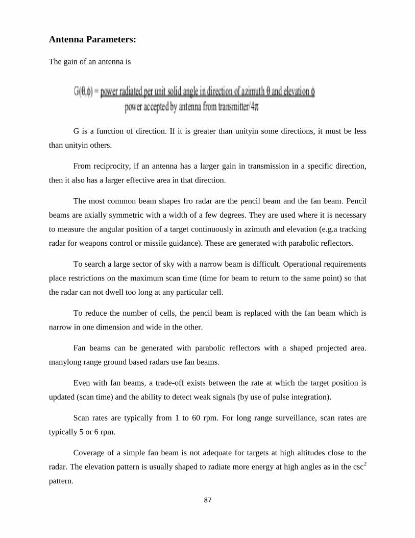
87

Antenna Parameters:

The gain of an antenna is

G is a function of direction. If it is greater than unityin some directions, it must be less

than unityin others.

From reciprocity, if an antenna has a larger gain in transmission in a specific direction,

then it also has a larger effective area in that direction.

The most common beam shapes fro radar are the pencil beam and the fan beam. Pencil

beams are axially symmetric with a width of a few degrees. They are used where it is necessary

to measure the angular position of a target continuously in azimuth and elevation (e.g.a tracking

radar for weapons control or missile guidance). These are generated with parabolic reflectors.

To search a large sector of sky with a narrow beam is difficult. Operational requirements

place restrictions on the maximum scan time (time for beam to return to the same point) so that

the radar can not dwell too long at any particular cell.

To reduce the number of cells, the pencil beam is replaced with the fan beam which is

narrow in one dimension and wide in the other.

Fan beams can be generated with parabolic reflectors with a shaped projected area.

manylong range ground based radars use fan beams.

Even with fan beams, a trade-off exists between the rate at which the target position is

updated (scan time) and the ability to detect weak signals (by use of pulse integration).

Scan rates are typically from 1 to 60 rpm. For long range surveillance, scan rates are

typically 5 or 6 rpm.

Coverage of a simple fan beam is not adequate for targets at high altitudes close to the

radar. The elevation pattern is usually shaped to radiate more energy at high angles as in the csc2

pattern.

88

Here φ0 and φm are the angular limits of the csc2φ fit

This pattern is used for airborne search radars observing ground targets as well as ground

based radars observing aircraft. For the airborne case φ is the depression angle. Ideally φm should

be 90˚ but it is always less. Csc2φ patterns can be generated bya distorted section of a parabola or

with special multiple horn feed on a true parabola, or with an array such as a slotted waveguide.

The csc2φ pattern gives constant echo power Pr independent of range for a target of

constant height, h and having a constant σ.

Substituting into the range equation (simple form)

Now for a constant height, h of a target, we have

Therefore Hence the echo signal is independent of range.

In practice Pr varies due to σ varying with viewing angle, the earth not being flat and non perfect

csc2φ patterns.

Note: the gain of csc2φ antennas for ground based radars is about 2 dB less than for a fan beam

having the same aperture.

The maximum gain of any antenna is related to its size by

Where ρ is the antenna efficiency which depends on the aperture illumination

This is controlled by the complexity of the feed design. Note: Aρ = Aeff

A typical reflector gives a beam width of where l is the dimension

89

System Losses:

Losses in the radar reduce the S/N at the receiver output. Losses which can be calculated

include the antenna beam shape loss, the collapsing loss and the plumbing loss. Losses which

cannot be calculated readily include those due to field degradation, operator fatigue and lack of

operator motivation.

Note: loss has a value greater than unity - Loss = [Gain]-1

1) Plumbing Loss

Loss in transmission lines between the transmitter and antenna and between

antenna and receiver.

Note from the Fig 2.28 that, at low frequencies, the transmission lines

introduce little loss. At high frequencies the attenuation is significant

Additional loss occurs at connectors (0.5 dB), bends (0.1dB) and at rotary joints

(0.4 dB)

Note: If a line is used for both transmission and reception, its loss is added twice.

The duplexer typically adds 1.5 dB insertion loss. In general, the greater the isolation

required, the greater the insertion loss.

90

2) Beam Shape Loss

The train of pulses returned from the target to a scanning radar are modulated in amplitude

by the shape of the antenna beam.

A beam shape loss accounts for the fact that the maximum gain is used in the radar equation

rather than a gain which changes from pulse to pulse. (This approach is approximate since it does

not address Pd for each pulse separately).

Let the one way power pattern be approximated by a Gaussian shape

Here θB is the half power beam width

nB is the number of pulses received within θB and if n is the number of pulses integrated, then

the beam shape loss (relative to a radar that integrated n pulses with equal gain) is

Example integrating 11 pulses gives L (beam shape) = 1.66 dB

Note: the beam shape loss above was for a beam shaped in one plane only (i.e. fan beam or

pencil beam where the target passes through the centre of the beam).

If the target passe through any other part of the beam the maximum signal will not

correspond to the signal from the beam centre.

When many pulses are integrated per beamwidth, the scanning loss is taken as 1.6 dB for

a fan beam scanning in one coordinate, and as 3.2 dB when two coordinate scanning is used.

When the antenna scans so rapidly that the gain on transmission is not the same as the

gain on reception, an additional “scanning loss” is added.

Additional loss for phased array search using a step scanning pencil beam since not all

regions of space are illuminated by the same value of antenna gain.

91

3) Limiting Loss

Limiting in radar can lower the Pd. This is not a desirable effect and is due to a limited

dynamic range. Limiting can be due to pulse compression processing and intensity modulation of

CRT (such as PPI).

Limiting results in a loss of onlya fraction of a dB for large numbers of pulses integrated

providing the limiting ratio (ratio of video limit level to RMS noise level) is greater than 2.

For small SNR in bandpass limiters, the reduction of SNR of a sine wave in narrowband

Gaussian noise is π/4 (approx 1 dB).

If the spectrum of the input noise is shaped correctly, this loss can be made ne gligible.

4) Collapsing Loss

If the radar integrates additional noise samples along with the wanted signal +noise pulses,

the added noise causes degradation called the collapsing g loss. This occurs on displays which

collapse range information (C scope which displays El vs Az).

In some 3D radars (range, Az, El) that displayoutputs at all Elevations on one PPI (range,

Az) display, the collapsing of the 3D information into 2 D display results in loss.

Can also occur when the output of a high resolution radar is displayed on a device which is of

coarser resolution than the radar.

Marcum has shown that for a square law detector, the integration of m noise pulses, along

with n signal + noise pulses with SNR per pulse (S/N)n, is equivalent to the integration of m+n

signal-to-noise pulses each with SNR of

The collapsing loss then is the ratio of the integration loss Li for m+n pulses to the

integration loss foe n pulses

92

Example: 10 signal pulses are integrated with 30 noise pulses Required Pd = 0.9, nf = 10

8

From Fig 2.8b. Li (40) = 3.5 dB, Li (10) = 1.7 dB

Therefore Li (m,n) = 1.8 dB

Collapsing loss for a linear detector can be much greater than for a square law detector.

Fig 2.29 shows the comparison of loss for each detector

5) Nonideal Equipment

Transmitter power - the power varies from tube to tube (for same type), and with age for a

specific tube. Power is also not uniform over the operating band. Hence Pt may be other than the

design value. To allow for this, a loss factor of about 2 dB can be used.

93

Receiver noise figure: the NF will vary over the band, hence if the best NF is used in the

radar equation, a loss factor must account for its poorer value elsewhere in the band.

Matched filter: if the receiver is not the exact matched filter fro the transmitted waveform, a

loss of SNR will occur (typically 1 dB).

Threshold level: due to the exponential relationship between Tfa and VT a slight change in

VT can cause significant change to Tfa hence, VT is set slightly higher than calculated to give

good Tfa in the event of circuit drifts. This is equivalent to a loss.

6) Operator Loss

A distracted, tired, overloaded, poorly trained operator will perform less efficiently. The

operator efficiency factor (empirical) is where Pd is the single scan probability of detection.

Note: operator loss is not relevant to systems where automatic detection is done

7) Field Degradation

When a radar is operated under field conditions, the performance deteriorates even more than

can be accounted for in the above losses.

Factors which cause field degradation are:

poor training

weak tubes

water in the transmission lines

incorrect mixer crystal current

deterioration in the receiver NF

poor TR tube recovery

loose cable connections

Radars should be designed with BIST (built - in system test) and BITE (built - in test

equipment) to aid in performance monitoring. A preventative maintenance plan should be used.

BITE parameters to be monitored are

Transmitted power Pt

94

NF of receiver

Transmitter pulse shape

Recovery time of TR tube

With no other information available, 3 dB is assumed for field degradation loss

8) Other Loss Factors

MTI radars introduce additional loss. The MTI discrimination technique results in complete

loss of sensitivity for certain target values (blind speeds).

In a radar with overlapping range gates, the gates may be wider than optimum for practical

reasons.

The additional noise introduced bynonoptimum gate width leads to degradation performance.

Straddling loss accounts for loss in SNR for targets not at the centre of a range gate, or at the

centre of a filter in a multiple bank processor

9) Propagation Effects

The radar equation assumes free space propagation. The earth’s surface and atmosphere have

a significant effect on radar performance.

The effects fall into three categories:

attenuation

refraction by the earth’s atmosphere

lobe structure caused by interference between the direct wave and the ground reflected

wave

For most microwave radars, attenuation through the normal atmosphere or through

precipitation is not significant. However reflection from rain (clutter) is a limiting factor in radar

performance in adverse weather.

The deceasing density of atmosphere with altitude results in bending (refraction) of the

electromagnetic wave. This normally increases the line of sight. the refraction can also be

95

accounted for by assuming the earth to have a larger radius than actual. A “typical” earth radius

is 4/3 actual radius.

At times atmospheric conditions create ducting (or super refraction) and increases the radar

range considerably. It is not necessarily desirable since it can not be counted on. Also it de

grades MTI performance by extending the range at which ground clutter is seen.

The presence of the earth also breaks the antenna elevation pattern into many lobes. this

arises since the direct and reflected waves interfere at the target either destructively or

constructively to produce nulls or lobes. This results in non uniform illumination.

Other Considerations:

The radar equation is now written.

Note: The following substitutions can be made:

Eτ = Pav/fp = Ptτ

N0 = N/B (power spectral density of noise)

Bτ ≈ 1 and T0Fn = Ts

Note: The above radar equation was derived for rectangular pulses but applies to other

waveforms provided that matched filter detection is used. The equation can be modified to

accommodate CW, FM-CW, pulse doppler MTI or tracking radar.

Radar Performance Figure - ratio of pulse power of Transmitter to Smin of receiver not

often used

Blip-Scan ratio - same as single scan Pd.

method used to check performance of ground-based radars

96

here an aircraft is flown on a radial course and for each scan of the antenna it is recorded

whether or not a target blip is detected. The ration of the number of scans the target was

seen at a particular range to the total number of scans is the blip scan ratio

head on and tail on aspects are easiest to provide.

Cumulative Probability of Detection:

If single scan probability of detection id Pd, the probability of detecting a target at least

once during N scans is the cumulative probability of detection

Pc = 1-(1-Pd)N

Note: the variation of Pd with range might have to be taken into account in computing Pc.

The variation with range based on the cumulative probability of detection can be the 3rd

power rather than the 4th

power which is based on a single scan probability. In practice Pc is not

easy to apply. Furthermore radar operators do not usually report a detection the first time it is

observed (which is required by the definition of Pc). Instead theyreport a detection based on

threshold crossing on two successive scans, or on two out of three scans.

For track while scan radars, the measure of performance might be the probabilityof

initiating a target track rather than just probability of detection.

Surveillance Radar Equation:

The radar equation which describes the performance of a radar which dwells on the target

for n pulses is sometimes called the searchlight range equation.

In a search or surveillance radar, the additional constraint that the radar must search a

specified volume of space in a specified time modifies the range equation significantly.

If Ω represents the angular region to be searched in scan time ts, then we have

Where t0 is the time on target = n/fp

Ω0 = solid angle beamwidth and Ω0 ≈ θAθE

97

Where θA is the Azimuth beamwidth And θE is the Elevation beamwidth

Also

With these substitutions the range equation becomes

This indicates that the important parameters for a search radar are the average power and

the antenna effective aperture.

Frequency does not appear explicitly, however low frequency is preferred since high

power and large aperture are easier to obtain at low frequencyand it is easier to build MTI

(moving target indicator) and weather has little effect on performance.

Note: the radar equation will be considerably different if clutter or external noise (jamming)

rather than receiver noise determine the background for the signal

Accuracy of the Radar Equation:

The predicted value of range from the range equation cannot be checked experimentally

with any accuracy. The safest means to achieve a specified range performance is to include a

safety factor. This is sometimes difficult to do in competitive bids but results in fine radars.

98

OBJECTIVE TYPE QUESTIONS

1. A high noise figure in a receiver means---------- [ ]

a. poor minimum detectable signal b. good detectable signal

c. receiver bandwidth is reduced d. high power loss.

2. Which of the following will be the best scanning system for tracking after a target has been

acquired.

a. conical b. spiral c. Helical d. Nodding

3. Which of the following noise figure. [ ]

a. (Si Ni) / (So No) b. (So No) / (Si Ni)

c. (So / No ) / sqrt. ( Si / Ni d. ( Si / Ni) / sqrt .(So / No

4. The average power of a pulsed radar transmitter is given by [ ]

a. The product of peak power of the pulse and the duty cycle

b. Peak power divided by the number of pulses repeated in one second.

c. Peak power divided by the duty cycle

d. Peak power divided by the duty cycle and pulse

5. Which of the following diode is used as detector in radar. [ ]

a. gunn diode b. schotky diode c. Impact diode d. varactor diode

6. In case the target cross section is changing the best system for accurate tracking is [ ]

a. monopulse b. lobe switching c. sequential lobing d. conical scanning.

7. In a radar in case the return echo arrives after the allocated pulse interval, then [ ]

a. it will not be received b. the receiver will get overloaded

99

c. it may interfere with the operation of the transmitter

d. the target will appear closer than it really.

8. PPI in a radar system stands for [ ]

a. plan position indicator b. pulse position indicator

c. plan position image d. prior position identification

9. Which of the following is unlikely to be used as a pulsed device [ ]

a. TWT b. BWO c. CFA d. Multicavity klystron

10. Radar detection is limited to line of sight because [ ]

a. curvature of the earth b. the waves are not reflected by the ionosphere

c. long wavelengths are used d. short wavelengths are used

11. Second time around echoes are caused by [ ]

a. Second time reflection from target

b. echoes returning from targets beyond the cathode ray tube range.

c. echoes that arrive after transmission of the next pulse.

d. extreme ends of bandwidth.

12. The resolution of pulsed radar can be improved by [ ]

a. increasing pulse width b. decreasing pulse width

c. increasing the pulse amplitude d. decreasing the pulse repetition frequency.

13. The most important application of monopulse antenna is in [ ]

a. determining the range of target b. tracking a target

c. identifying a target d. Isolating the track of target.

100

14. In case the antenna diameter in a radar system is increased to four times. The maximum

range will increase by [ ]

a. √2 times b. 2 times c. 4 times d. 8 times.

15. In case the ratio of the antenna diameter to the wavelength in a radar system is high, this is

likely not to result in [ ]

a. increased capture area b. good target discrimination

c. difficult target acquisition d. large maximum range

16. The term RADAR stands for [ ]

a. radio direction and reflection b. radio detection and ranging

c. radio waves dispatching and receiving d. random detection and re radiation.

17. The duty cycle in a pulsed radar transmitter cannot be increased beyond a point because it

a. affects the operating frequency

b. increase the average power of the transmitter tube.

c. does not detect weak signals

d. increase minor lobes

18. In case of radar receiver the IF bandwidth is inversely proportional to [ ]

a. pulse interval b. pulse repetition frequency

c. square root of the peak transmitted power d. pulse width.

19. The Doppler effect is used in [ ]

a. MTI b. CW c. FM d. Radar Altimeter

20. The gain of a radar transmitting antenna is [ ]

a. loss than that of radar receiving antenna

101

b. almost equal to that of radar receiving antenna

c. slightly higher than that of radar receiving antenna

d. much higher than that of radar receiving antenna.

Answers:

1.a 2.a 3.a 4.a 5.c 6.a 7.d 8.b 9.b 10.a

11.c 12.b 13.b 14.c 15.a 16.b 17.b 18.d 19.d 20.d

ESSAY TYPE QUESTIONS

1. Describe how threshold level for detection is decided in the presence of receiver noise for

a specified probability of occurrence of false alarms.

2. Describe the e ect of pulse repetition frequency on the estimated unambiguous range of

radar.

3. Obtain yhe SNR at the output of IF amplifier of radar receiver for a specified probability

of detection without exceeding a specified probability of false alarm.

4. Explain system losses will effect on the radar rangr?

5. Discuss about the factors that influence the prediction of radar range.

6. Define noise bandwidth of a radar receiver. How does it differ from 3 db band width?

Obtain the expression for minimum detectable signal in terms of noise bandwidth, noise

figure and other relavent parameters.

7. If the noise figure of a receiver is 2.5 db, what reduction (measured in dB) occurs in the

signal noise ratio at the output compared to the signal noise ratio at the input?

8. Describe the e ect of (in terms of wavelength of operation) size of a simple spherical target

on determination of radar cross section of the sphere.

9. What are multiple-time-around echoes? Explain the relation between unam-biguous range

estimation and multiple-time-around echoes.

10. Establish a relation between the probability of false alarm and detection threshold level of

102

a radar receiver in the presence of noise.

11. Estimate the radar cross-section of a spherical target if the wavelength of transmitting

signal with reference to the target size is in Rayleigh region.

12. Justify the requirement of integration of radar pulses to improve target detection process.

13. List all the possible losses in a radar system and discuss the possible causes of each of

them.

14. Discuss about the factors that in uence the prediction of Radar range.

15. De ne noise bandwidth of a radar receiver. How does it di er from 3-dB bandwidth?

Obtain the expression for minimum detectable signal in terms of noise bandwidth, noise

figure and other relevant parameters.

16. Explain the principle and process of binary moving window detector.

17. Obtain the SNR at the output of IF ampli er of Radar Receiver for a specified probability

of detection without exceeding a specified probability of false alarm.

18. Explain how system losses will a effect on the Radar Range?

19. Determine the probability of detection of the Radar for a process of threshold detection

with a graphic illustration.

20. Determine the Radar cross-section of a cone sphere.

103

UNIT-III

CW AND

FREQUENCY

MODULATED

RADAR

104

CW radar detects objects and measures velocity from Doppler shift.

CW radar sets transmit a high-frequency signal continuously.

It can not measure range.

It can be mono-static or bi-static.

Employs continual RADAR transmission

Separate transmit and receive antennas

Relies on the “DOPPLER SHIFT”

105

Pulse Transmission

Continuous Wave

106

PRINCIPLE OF DOPPLER EFFECT:

The radars radiate electromagnetic waves towards the targets for detection and also to

obtain details of the target.

When the target is stationary, the frequency of the received echoes is constant.

However, when the target is moving, the frequency of the received echoes is found to be

different from transmitted frequency.

If the target approaches the radar, the frequency is increased and if the target moves away

from the radar, the frequency is decreased.

That is, in the moving targets, there exists a frequency shift in the received echo signals.

The presence of frequency shift in the received echo signals in the radar due to moving

targets is known as Doppler Effect.

The frequency shift is known as Doppler frequency shift

Doppler Effect:

When there is a relative motion between Radar and target is based on recognizing the

change in the echo-signal frequency caused by the Doppler Effect.

If either obser or the source is in motion, then it results in a frequency shift, the resulatent

frequency shift is known as Doppler Effect.

When an observer moves relative to a source, there is an apparent shift in frequency is

known as Doppler frequency.

If distance between observer and the source is increasing, the frequency apparently

decreses, where as the frequency apprantly increases if the distance between the observer and the

source is decreasing is known as Doppler frequency.

If R is the distance from Radar to target, the total number of wavelengths λ contained in

the two-way path between the Radar and target is 2R/λ. i.e., the total number of wave lengths

=

.

Since one wavelength corresponds to an angular excursion of 2π radians, the total angular

excursion of φ made by the electromagnetic wave during its transit to and from the target is

radians. Therefore, φ = 2π×total number of wavelengths = 2π×

=

radians.

107

If the targe is in motion, distance R and phase φ are continually changing. Achange in φ

with respect to time is equal to a frequency. This is the Doppler angular frequency ωd and it is

given by ωd = 2πfd =

=

=

=

= 4πvr/λ

2πfd = 4πvr/λ

fd = 2vr/λ fd = 2vr/λ

Where fd = Doppler frequency shift in hertz

vr = relative velocity or radial velocity of target with respet Radar in knots.

= dR/dt

λ = wavelength in meters = c/f0

The distance R and wavelength λ are measured in same units.

The Doppler frequency shift is fd = 2vr/λ = 2vr/( c/f0)

fd = 2vrf0/c =

fd = 2vrf0/c

Where f0 = transmitted frequency

c = velocity of propagation = 3×108 m/sec.

If fd in Hz, vr in knots and λ in meters: fd = 1.03vr/λ fd = 1.03vr/λ

The relative velocity may be written vr = vcosθ

Where v is the target speed and θ is the angle made by the target trajectory and the line joining

Radar and target.

Therefore, fd = 2vcosθ/λ

When θ = 00, the Doppler frequency is maximum. The Doppler frequency is zero, when

the trajectory is perpendicular to the Radar line of sight (θ = 900).

CW RADAR:

A Simple CW Radar is shown in fig1 (a). The CW Radar consists of a transmitter,

detector, beat-frequency amplifier and indicator.

The transmitter transmits a continuous wave of frequency oscillation or oscillation of

frequency f0, which is radiated by the antenna. An amount of radiated energy is intercepted by

108

the target and some of this energy is scattered back in the direction of the Radar. This energy is

collected by the receving antenna.

f0

f0±fd f0±fd f0

fd fd

Fig 1(a): Simple CW Radar Block Diagram

Response

Frequency

Fib 1(b): Response characteristic of beat-frequency amplifier

If the target is in motion with a relative velocity vr to the Radar, then the received signal

will be shifted by an amount of ‘±fd’.

The plus sign associated with the Doppler frequency applies if the distance between

target and Radar is decreasing (closing target), i.e., when the received signal frequency is greater

than the transmitted signal frequency. The minus sign associated with the Doppler frequency

applies if the distance between target and Radar is increasing (receding target), i.e., when the

received signal frequency is less than the transmitted signal frequency.

CW

Transmitter

f0

Detector Or

Mixer

Beat Frequency Amplifier

Indicator

Detector

Or Mixer

Beat

Frequency

Amplifier

Indicator

109

The received echo signal at a frequency f0±fd enters the Radar via the antenna and is

heterodyne in the detector with a part of the transmitted signal f0 to produce a Doppler beat

frequency fd. The sign is lost in this process.

The purpose of Doppler amplifier is to eliminate the echos from stationary targets and to

amplify the Doppler echo signal to a level where it can be used to operate an indicating device. It

must have a frequency characteristic similar to that of fig1 (b).

The low frequency cut-off must be high enough to reject the dc component caused by

stationary targets. The upper cut-off frequency is selected to pass the higest Doppler frequency

expected. Finally, an indicator deviceis used, generally it consists of a pair of earphones or a

frequency meter.

Isolation between transmitter and receiver:

The main impotance of providing isolation between transmitter and receiver is to

eliminate the transmitter leakage signal.

Generally separate antennas are used for transmission and reception, so that there is no

chance of leakage entering the receiver. Even the isolation between transmitter and receiver is

possible using a single antenna as in CW Radar.

The noise that accompanies the transmitter leakage signal will determine the amount of

isolation needed in a long range CW Radar. For example, a 10 mwatt of leakage signal is

appeared at the receiver for a proper isolation between transmitter and receiver. The transmitter

noise must be atleast 110 dB beliw the transmitted carrier for a minimum detectable signal of 10-

13 watt.

The isolation between transmitter and receiver can be obtained with a single antenna (like

CW Radars) by using a hybrid junction, circulator, turnstile junction or with separate

polarizations. Even though the isolation achieved by hybrid junctions such as magic Tee, rat race

or directional coupler is 60 dB in extreme cases, the isolation in practical cases is limited 20 or

30 dB.

110

The limitation of 6dB on overall performance using junctions is going to waste half the

transmitted power and half the received power. Thus, hybrid junctions are applicable to short

range Radars. Similarly, ferrite isolaton devices and turnstile junctions are also limited to short

range Radar due to the difficulty in obtaining large isolations.

The large isolatons are obtained in CW tracker-illuminator using separate antennas for

transmission and reception. By the proper insertion of a controlled sample of the transmitted

signal directly into the receiver, additional isolation can be obtained. The part of transmitted

signal that leaks into the receiver can be cancelled by adjustin the phase and amplitude of the

“buck-off” signal. The arrangement introduces aditional 10dB isolation. But the phase and

amplitude of the leakage signal may vary as the antenna scans. Thus a dynamic canceller can be

used that senses the proper phase and amplitude of leakage signal for obtaining the additional

isolation. Thus, the above dynamic cancellation of leakage signal can exceed isolation to 30dB.

Intermediate-Frequency Receiver:

The receiver of the simple block diagram of CW Radar is in some respect analoguos to a

superheterodyne receiver. Receivers of this type are called homodyne receivers or

superheterodyne receivers with zero.

The function of the local oscillator is replaced by the leakage signal from the transmitter.

Such a receiver is simpler than one with a more conventional intermediate frequency since no IF

amplifier or local oscillaotor is requied. However, the simple receiver or zero IF receiver is not

as sensitive because of increased noise at lower intermediate frequency caused by flicker effect.

Flicker effect noise occurs in semiconductor devices such as diode detector and cathods

of vacuume tubes. The noise power produced by flicker effect varies as 1/fα, where α is

approximately unity.

The fig (2) shows a block diagram of CW Radar whose reciver operates with a non-zero

IF. In this case, separate antennas are shown for transmission and reception. Instead of the local

oscillator determined in the conventional superheterodyne receiver, the local oscillator or

reference signal is derived in this receiver from a part of transmitted signal mixed with a locally

111

generated signal of intermediate frequency fif to generate the two side bands f0+fif and f0-fif along

with f0 and higher harmonics.

f0

Transmitting Antenna

f0

fif

f0, f0+fif and f0-fif

Receiving Antenna f0+fif

fif±fd

f0±fd

fd

Fig (2): Block diagram of CW Doppler Radar with non-zero IF receiver, some times

called side-band superheterodyne.

From this signal one of the side band is selected by passing it through narrowband filter

as the reference signal.

The reference signal from the sideband filter is mixed with the signal from receiving

antenna to get the intermediate signal fif±fd which is amplified and then applied to the second

detector to get the Doppler echo signal fd.

CW

Transmitter

f0

Mixer

Side-band

Filter

Receiver

Mixer

Oscillator

fif

IF

Amplifier

Second

Detector

Doppler

Amplifier Indicator

112

The purpose of Doppler amplifier is to eliminate the echos from stationary targets and to

amplify the Doppler echo signal to a level where it can be used to operate an indicating device,

such as a pair of earphones or a frequency meter.

Comparision between zero and non-zero IF receivers:

1. Zero IF receiver is not as sensitive because of increased noise at lower intermediate

frequency caused by flicker effect.

2. The reduction in sensitivity has greater effect on the maximum efficiency with CW

Radar.

3. The improvement in receiver sensitivity with an non-zero IF receiver might be around

30 dB over the zero IF receiver.

Receiver Bandwidth:

The factors which tend to spread to the CW signal energy over a finite band of

frequencies are discussed in the following.

If the received waveform were a sine infinite duration, its frequency spectrum would be

a delta function and the receiver bandwidth would be infinitesimal. But a sine wave of infinite

duration and an infinitesimal bandwidth does not exist in nature. So, considering an echo signal

which a sine wave of finite duration rather than infinite duration. Then the spectrum of finite

duration sine wave is given by sin[π(f-f0)δ]/π(f-f0)

Where f0 = frequency of sine wave

δ = duration of sine wave

f = frequency variable over which is spectrum is plotted as shown in fig (3b).

The above characteristic is approximated by the practical receivers. In practical aspects,

the echo may not be a pure sine wave, so we need to broaden the bandwidth still further.

Assuming that for a CW Radar, the duration of the received signal is given by δ = θB/θ.S

113

i.e., time taken on target = δ = θB/θ.S

Where θB = antenna beamwidth in degrees and θ.S = antenna scaning rate in degrees/sec

Thus, the signal is of finite duration and bandwidth of the receiver must be of the order of

the reciprocal of the time on target θ.S/θB. For example, if the antenna beamwidth and antenna

scaning rate are 20 and 36

0/sec (6 rpm) respectively. Then the spread in the spectrum of the

received signal due to the finite time on the target is 18 Hz, which is independent of the

transmitted frequency.

In addition to the spread of the received signal spectrum caused by the finite time on the

target, the spectrum may be further widened, if the target cross section fluctuates.

Energy/Hz of bandwidth Energy/Hz of bandwidth

∆f=1/δ

f0 Frequency f0 Frequency

(a) Infinite duration (b) Finite duration

Fig(3): Frequency spectrum of CW oscillation

The echo signal from a propeller driven aircraft can also contain modulation component

at a frequency proportional to the propeller rotation.

The frequency range propeller modulation depends upon the shaft rotation speed and the

number of propeller blades. Propeller may cause an error in measurement of Doppler frequency.

This modulation may also be advantageous in the detection of propeller driven aircraft by

passing tangential trajectory even in the absence of Doppler frequency shift.

114

The modulation of echo signal is also resulted by rotating blades of a helicopter and the

compressor stages of a jet ebgine and which will degrade the performance of the CW Radar by

widening the soecrum.

A further widening of the received signal spectrum can occur, if the relative velocity of

the target is not constant. If ar is the acceleration of the target with respect to the Radar, the

signal will occupy a bandwidth: ∆fd = (2ar/λ) 1/2

If for example, ar is twicw the acceleration of gravity, the receiver bandwidth must be

approximately 20 Hz when Radars wavelength is 10cm.

Filter Bank in CW Radar receiver:

A relative wide band of frequencies called as bank of narrow band filters are used to

measure the frequency of echo signal. These are also used to improve the signal to noise ratio of

the receiver. The bandwidth of each individual filter is such that, it accepts the signal energy but

should be taken that it does not introduce more noise because of wide bandwidth.

The center frequencies of the filters are staggered to cover the entire range of Doppler

frequencies. If the filters are spaced with their halh power points overlapped, the maximum

reduction in signal to noise ratio of a signal which lies midway between adjacent channels

compared with the signal to noise ratio at midband is 3 dB. By using the large number of filters,

the maximum loss will be reduced but it increases the probability of false alaram. The fig 4(a)

shows the block diagram of IF Doppler filter bank.

A bank of narrow band filters may be used after the detector in the video of the simple

CW Radar, instead of in the IF. The improvement in signal to noise ratio with a video filter bank

is not as good as can be obtained with an IF filter bank, but the ability to measure the magnitude

of Doppler frequency is still preserved.

The sign of the Doppler shift is lost with a video filter bank and it can not be directly

determined whether the Doppler frequency corresponds to an approaching or to a receding target.

115

One advantages of the foldover in the vedio is that only half the numer of filters are required than

in the IF filter bank. The equivalent of a bank of continguous bandpass filters may also be

obtained by converting the analog IF or vedio signal to a set of sampled, quantized signals which

are processed with digital circuitry by means of the fast Fourier transform algorithm.

Fig 4(a): Block diagram of IF Doppler filter bank

Response

IF Bandwidth

f1 f2 f3 f4 fn Frequency

Fig 4(b): Frequency-Response characteristic of Doppler filter bamk

Filter No.1 Detector

Filter No.2

Detector

Filter No.3

Detector

Filter No.4

Detector

Filter No.n

Detector

IF amplifier Mixer

I

N

D

I

C

A

T

O

R

116

The complexity of the receiver is increased by the bank of overlapping Doppler filters whether in

IF or vedio. The bank of Doppler filters may be replaced by a narrowband tunable filter, when

the system requirements permit a time sharing of the Doppler frequency range.

Measurement of Doppler direction with CW Radar OR Sign of Radial

Velocity:

In some applications of CW Radar it is of interest to know whether the target is approaching or

recedind. This might be determined with separate filters located on either side of the intermediate

frequency.

If the echo signal frequency lies below the carrier, the target is receding. If the echo signal

frequency is greater than the carrier, the target is approaching, which is shown in fig (5).

Amplitude Amplitude Amplitude

fd fd

f0 Frequency f0 Frequency f0 Frequency

Fig(5): Spectra of received signal. (a) No Doppler shift, no relative target motion,

(b) Approching target and (c) Receding target

Although the Doppler frequency spectrum “folds over” in the vedio because of the action of the

detector, it is possible to determine its sign from a technique borrowed from single sideband

communications.

If the transmitter signal is given by Et = E0 cos (ω0t)

The echo signal from a moving target will be Er = k1E0 cos [(ω0±ωd)t+φ]

Where E0 = amplitude of transmitted signal

k1 = a constant determined from the Radar equation

ω0 = angular frequency of transmitter in rad/sec

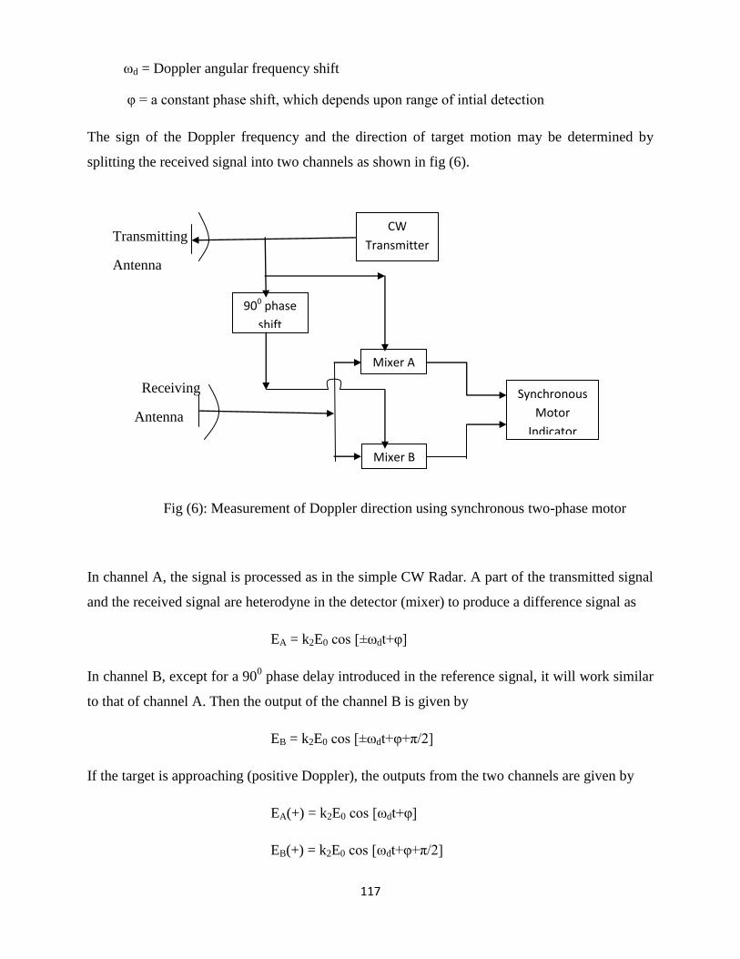
117

ωd = Doppler angular frequency shift

φ = a constant phase shift, which depends upon range of intial detection

The sign of the Doppler frequency and the direction of target motion may be determined by

splitting the received signal into two channels as shown in fig (6).

Transmitting

Antenna

Receiving

Antenna

Fig (6): Measurement of Doppler direction using synchronous two-phase motor

In channel A, the signal is processed as in the simple CW Radar. A part of the transmitted signal

and the received signal are heterodyne in the detector (mixer) to produce a difference signal as

EA = k2E0 cos [±ωdt+φ]

In channel B, except for a 900 phase delay introduced in the reference signal, it will work similar

to that of channel A. Then the output of the channel B is given by

EB = k2E0 cos [±ωdt+φ+π/2]

If the target is approaching (positive Doppler), the outputs from the two channels are given by

EA(+) = k2E0 cos [ωdt+φ]

EB(+) = k2E0 cos [ωdt+φ+π/2]

CW

Transmitter

900 phase

shift

Mixer A

Mixer B

Synchronous

Motor

Indicator

118

If the target is receding (negative Doppler), the outputs from the two channels are given by

EA(-) = k2E0 cos [-ωdt+φ] OR EA(-) = k2E0 cos [ωdt-φ]

EB(-) = k2E0 cos [-ωdt+φ+π/2] OR EB(-) = k2E0 cos [ωdt-φ-π/2]

The sign of Doppler frequency and the direction of target’s motion may be determined according

to whether the output of channel B leads or lags the output of channel A.

The approximation of two channel output to a synchronous two phase motor is one the method of

determining relative phase relationship between them. In which, the direction of the target motin

is indicated by the direction of motor rotation.

The relarive phase of the two channels can be sensed by other electronic methods instead of a

synchronous motor. Using this technique we can determine the velocity of theaircraft with

respect to the ground take-off and landing. Thus, in this way we can identify the Doppler

direction with respect to CW Radar.

CW Tracking Illiminator:

XTAL

X+D

X

X

XTAL

Pedestal Control

Fig (7): Block diagram of a CW tracking illuminator

Phase

Compensato

r

Servo

System

Scan

Detector

Speed Gate Doppler

Amplifier

Signal IF

Magnetron Klystron AFC

Reference IF

119

The figure shows the basic block diagram oc CW tracking illuminator. It is a tracking Radar as

well as illuminator. Since it must be able to follow the target as it travels through space. The

operation in presence of clutter is possible, due to the Doppler discrimination of continuous wave

Radar. In this type of Radar, the receiver in the missile receives the energy from the target and

this energy has been transmitted to the missile by an illuminator. The illuminator may be at the

launch platform. This CW illuminator has been used in many successful systems. Speed gate is a

wide band Doppler amplifier shown in fig (7), which is also referred as narrowband tracking

filter. The main function of this gate is to acquire the target and track, by changing Doppler

frequency shift.

Advantages of CW Doppler Radar:

1. CW Doppler Radars are not pulsed and simple to manufacture.

2. These Radars have no minimum or maximum range and maximize power on a target

because they are always broad casting.

3. These are having the ability to measure velocity with extreme accuracy by means of the

Doppler shift in the frequency echo.

4. The detected, reflected wave is shifted in frequency by an amount which is a function of

the relative velocity between the target and the transmitter receiver.

5. Range data are extracted from the change in Doppler frequency.

Disadvantages of CW Doppler Radar:

1. When a single antenna is used for both transmission and reception, it is difficult to protect

the receiver against the transmitter because in constant to pulse Radar, both are ON all

the time.

2. These are able to detect only moving targets, as stationary targets will not cause a

Doppler shift and the reflected signals will be filtered out.

3. CW Radars are not able to measure range, where range is normally measured by timing

the delay between a pulse being sent and received but as CW Radars are always

broadcasting; there is no delay to measure.

120

Applications of CW Doppler Radar:

1. Simple unmodulated CW Radar can be used to find the relative velocity of a moving

target without any physical constant with the target. For example: in police speed

monitors, in rate of climb-meter for vertical-take-off aircraft, measurement of turbine-

blade vibration, the peripheral speed of grinding wheels and the monitoring of vibrations

in the cables of suspension bridges.

2. CW radars are also used for the control of traffic lights, regulation of toll booths, vechical

counting.

3. In railways CW Radars can use as a speed meter to replace the conventional axle-driven

tachometer.

4. In measurement of rail roadfrieght car velocity during humping operations in marshalling

yards.

5. It can also be used as detection device to give track maintenance personnel advance

warning of approaching trains.

6. It is also employed for monitoring the docking speed of large ships.

Pulse Vs. Continuous Wave:

Pulse Echo Continuous Wave

1. Single Antenna

2. Gives Range, usually Alt. as well

3. Susceptible To Jamming

4. Physical Range Determined By PW and

PRF.

1. Requires 2 Antennae

2. Range or Alt. Info

3. High SNR

4. More Difficult to Jam But Easily

Deceived

5. Amp can be tuned to look for expected

frequencies

121

Unambiguous Range in CW Radar:

Consider a CW Radar with the folling waveform S(t) = A sin(2πf0t)

The received signal from moving target at range is Sr(t) = Ar sin(2πf0t-φ)

Where the phase φ = 2πf0T

But, R=cT/2

T=2R/c and λ=c/f0

Therefore, φ = 2πf0(2R/c) = 4πf0R/c= 4πR/λ

R = λφ/4π ------- (1)

Where, c is the velocity of propagation = 3×108 m/sec.

From the above equation we observe that, the maximum unamgiguious range occurs when φ is

maximum i.e., φ=2π. Therefore, even for relatively large Radar wavelength R is limited to

impractical small values.

Now consider a Radar with two CW signals denited by S1(t) and S2(t) respectively.

S1(t) = A1 sin(2πf1t) and S2(t) = A2 sin(2πf2t)

The received signal from moving target at range is S1r(t) = Ar1 sin(2πf1t-φ1)

S2r(t) = Ar2 sin(2πf2t-φ2)

Where φ1 = 2πf1(2R/c) = 4πf1R/c and φ2 = 2πf2(2R/c) = 4πf2R/c

After mixing the carrier frequency, the phase difference between the two received signals is

∆φ = φ2-φ1

∆φ = (4πf2R/c)-(4πf1R/c) = (4πR/c)( f2-f1)

∆φ = (4πR/c)(∆f) = 4πR∆f/c

After R is maximum when ∆φ = 2π

122

Therefore ∆φ = 4πR∆f/c => 2π = 4πR∆f/c

R = c/2∆f -----------(2)

Since, ∆f<<c, the range computed by eq(2) is such greater than that computed by eq(1).

Prob (1): For an ambiguious range of 81 nautical miles (1nmi=1852 meters) in a two

frequency CW Radar. Determine f2 and ∆f when f1=4.2 kHz.

Sol: Given that, unambiguious range R = 81 nmi

Runamb = 81×1852=150.012 km

The unambiguious range R = c/2∆f = 999.92 Hz

∆f = f2-f1

f2=∆f+f1=5.199 kHz

Prob (2): Determine the acceleration of a target if the received signal bandwidth is 40 Hz and

the operating wavelength is 9 cm.

Sol: Given that for a moving target

Received signal bandwidth ∆fd=40Hz

Operating wavelength = 9cm = 9×10-2

m

Acceleration of a target ar=?

We know that, ∆fd = (2ar/λ)1/2

ar=72 m/sec2

Prob (3): Determine the operating wavelength if the target is moving with acceleration as same

as acceleration of gravity and the received signal bandwidth is 50 Hz.

Sol: Given that, acceleration of a moving target ar=9.8 m/sec2 = acceleration of gravity

123

Received signal bandwidth ∆fd=50Hz

Operating frequency = ? and λ = c/f0

We know that, ∆fd = (2ar/λ)1/2

f0=38.27 Hz.

Prob (4): with atransmit (CW) frequency of 5GHz, calculate the Doppler frequency seen by

stationary Radar when the target radial velocity is 100km/hr.

Sol: f0=5GHz, vr=100km/hr = 100×5/18 m/sec = 27.778 m/sec.

The Doppler frequency, fd = 2vrf0/c = 925.93 Hz.

124

OBJECTIVE TYPE QUESTIONS

1. Stagger PRF is used to [ ]

a. shift the target velocities to which the MTI system is blind

b. improves the detection of a moving target against cluster background

c. increase the average power transmitted

d. increase the peak power transmitted.

2. COHO stands for [ ]

a. coherent output b. counter housed oscillator

c. coherent local oscillator d. carrier oscillater and harteley oscillater

3. If the peak transmitted power in a radar system in increased by a factor of 16, the maximum

range will be increased [ ]

a. 2 times b. 4 times c. 4 times d. 16 times

4. Which of the following statement is incorrect.The radar cross section of a target? [ ]

a. depends on the aspect of a target, if this is non spherical.

b. depends on the frequency used.

c. is equal to the actual cross sectional area for small targets

d. may be reduced by special coating of the target.

5. Which of the following statement is incorrect High PRF will [ ]

a. increase the maximum range

b. make target tracking easier to distinguish from noise

c. make the retured echoes easier to distinguish from noise

d. have no effect on the range resolution.

125

6. Side lobe of an antenna causes [ ]

a. reduction in gain of antenna b. reduction in beam width of antenna

c. ambiguity in direction finding d. increases directivity

7. A radar which is used for determining the velocity of the moving aircraft along with its

position and range is [ ]

a. moving target indicator b. radar speedometer

c. pulse radar d. radar range finder

8. Blind speed in MTI radar results in [ ]

a. restriction in speed of detectable targets b. blanking to PPI.

c. no change in phase detector output d. absorption of electromagnetic waves.

9. The quartz delay line in a MTI radar is used to [ ]

a. match the signal with echo b. substract a complete scan from previous scan

c. match the phase of COHO and STALO

d. Match the phase of COHO and output of oscillator

10. Which one of the following applications or advantages of radar beacons is false [ ]

a. navigation b. target identification

c. more accurate tracking of enemy target

d. very significant extension of the maximum range.

11. STALO stands for [ ]

a. standard local oscillator b. stable L-band output

c. stabilized local oscillator d. saturated and linear oscillator.

12. Large antenna is used in radar because it [ ]

126

a. gives higher gain b. gives lesser side lobes.

c. increases the bean width d. increases band width

13. The range of radar is [ ]

a. directly proportional to the gain of the radar antenna

b. directly proportional to the minimum detectable signal by the receiver

c. inversely proportional to the gain of the radar antenna

d. inver4sely proportional the transmitted power.

14. A biostatic radar has [ ]

a. one antenna for transmitting as well as for receiving

b. two antennas for receiving the signal. c. two antennas for transmitting signal

d. transmitting and receiving antennas

15. Blind speed causes target to appear [ ]

a. moving uniformly b. moving irregularly c. stationary d. intermittently

16. For precise target location and tracking retards operate in ` [ ]

a. s- band b. D- Band c. L- Band d. X - Band

17. The sensitivity of a radar receiver is ultimately set by [ ]

a. high S/N ratio b. lower limit of useful signal input

c. overall all noise temperature d. low S/N ratio

18. A radar system cannot be used [ ]

a. to detect moving objects b. to detect trajectory of moving objects

c. to detect aircraft d. to detect storms

19. Which of the following is essential for fast communication [ ]

127

a. Hgh S/N ratio b. High channel capacity

c. large bandwidth d. Higher directivity

20. The major advantage of pulsed radar CW radar is that [ ]

a. pulsed radar readily gives the range of target while CW radar cannot give range

information

b. pulsed radar can identify a target more easily than CW radar.

c. Pulses get reflected from the target more efficiently as compared to CW waves

d. Pulses have variation of magnitude and frequency both

Answers:

1.a 2.c 3.a 4.c 5.a 6.a 7.c 8.a 9.b 10.c

11.c 12.a 13.b 14.d 15.c 16.a 17.c 18.d 19.a 20.a

ESSAY TYPE QUESTIONS

1. With the help of a suitable block diagram, explain the operation of CW Doppler radar in a

sideband super heterodyne receiver.

2. Calculate the Doppler frequency of stationary CW radar transmitting at 6 MHz frequency

when a moving target approaches the radar with a radial velocity of 100 Km/Hour.

3. List the limitations of CW radar.

4. What is Doppler frequency shift? Establish a relation between Doppler frequency shift and

radial velocity of a moving target.

5. Explain how isolation between transmitter and receiver of a radar system can be achieved

128

if single antenna is used for transmission and reception.

6. What is Doppler frequency shift? Discuss the e ect of receiver bandwidth on the e ciency

of detection and performance of a CW Doppler radar.

7. With the help of a suitable block diagram, explain the operation of a CW tracking

illuminator application of a CW radar.

8. With the help of a suitable block diagram, explain the operation of a CW radar with non-

zero IF in the receiver.

9. Describe methods to achieve isolation between transmitter and receiver of a CW Doppler

radar if same antenna is to be used for transmission and reception

10. What is the beat frequency? How it is used in FMCW radar?

11. Explain how the multipath signals produce error in FM altimeter?

12. Explain how earphones are used as an indicator in CW Radar?

13. The transmitter power is 1 KW and safe value of power which might be applied to a

receiver is 10mW. Find the isolation between transmitter and receiver in dB. Suggest the

appropriate isolator.

14. Why the step error and quantization errors which occur in cycle counter are used for

frequency measurement in FMCW Radar?

15. What is the Doppler effect? What are some of the ways in which it manifests itself? What

are its radar applications?

16. Find the relation between bandwidth and the acceleration of the target with respect to

radar?

17. How to find the target speed from Doppler frequency?

18. Write the applications of CW Radar.

19. What are the factors that limit the amount of isolation between Transmitter and Receiver

of CW Radar?

20. Explain how earphones are used as an indicator in CW Radar?

21. The transmitter power is 1 KW and safe value of power which might be applied to a

receiver is 10mW. Find the isolation between transmitter and receiver in dB. Suggest the

appropiate isolator.

129

UNIT-IV

FM-CW

RADARR

130

Frequency-Modulated Continuous-Wave Radar:

CW radars have the disadvantage that they cannot measure distance, because it lacks the timing

mark necessary to allow the system to time accurately the transmit and receive cycle and convert

the measured round-trip-time into range. In order to correct for this problem, phase or frequency

shifting methods can be used. In the frequency shifting method, a signal that constantly changes

in frequency around a fixed reference is used to detect stationary objects and to measure the rage.

In such Frequency-Modulated Continuous Wave radars (FMCW), the frequency is generally

changed in a linear fashion, so that there is an up-and-down or a sawtooth-like alternation in

frequency. If the frequency is continually changed with time, the frequency of the echo signal

will differ from that transmitted and the difference Δf will be proportional to round trip time Δt

and so the range R of the target too. When a reflection is received, the frequencies can be

examined, and by comparing the received echo with the actual step of transmitted frequency, you

can do a range calculation similar to using pulses:

transmitted signal

received

echo signal

131

R = c0|Δt|/2= c0|Δf|/(2df/dt)

Where: c0 = speed of light = 3·108 m

/s

Δt = measured time-difference [s]

R = distance altimeter to terrain [m]

df/dt = transmitters frequency shift per unit time

Characteristic Feature of FMCW radar:

1. The distance measurement is done by comparing the actual frequency of the received

signal to a given reference (usually direct the transmitted signal)

2. The duration of the transmitted signal is much larger than the time required for measuring

the installed maximum range of the radar

Doppler direction in FMCW radar:

A block diagram illustrating the principle of the FM-CW radar is shown in Fig. A

portion of the transmitter signal acts as the reference signal required to produce the beat

frequency. It is introduced directly into the receiver via a cable or other direct connection. Ideally

the isolation between transmitting and receiving antennas is made sufficiently large so as to

reduce to a negligible level the transmitter leakage signal which arrives at the receiver via the

coupling between antennas. The beat frequency is amplified and limited to remove any

amplitude fluctuations. The frequency of the amplitude-limited beat note is measured with a

cycle-counting frequency meter calibrated in distance.

Fig: Block diagram of FM-CW radar

132

In the above, the target was assumed to be stationary. If this assumption is not applicable,

a Doppler frequency shift will be superimposed on the FM range beat note and an erroneous

range measurement results.

The Doppler frequency shift causes the frequency-time plot of the echo signal to be

shifted up or down (Fig. 4.1.2 (a)). On one portion of the frequency-modulation cycle the heat

frequency (Fig, 4.1.2 (b)) is increased by the Doppler shift, while on the other portion it is

decreased. If for example, the target is approaching the radar, the beat frequency fb(up) produced

during the increasing, or up, portion of the FM cycle will be the difference between the beat

frequency due to the range fr, and the doppler frequency shift fd. Similarly, on the decreasing

portion, the beat frequency, fb(down) is the sum of the two.

fb(up) = fr - fd and fb(down) = fr + fd

The range frequency fr, may be extracted by measuring the average beat frequency;

That is, fr = 1/2[fb(up) + fb(down)].

133

Fig: Frequency-time relation-ships in FM-CW radar when the fr + fd received signal is shifted

in frequency by the doppler effect (a) Transmitted (solid curve) and echo (dashed curve); (b) beat

frequency.

If fb(up) and fb(down) are measured separately, for example, by switching a frequency

counter every half modulation cycle, one-half the difference between the frequencies will yield

the doppler frequency. This assumes fr > fd.

If, on the other hand, fr < fd such as might occur with a high-speed target at short range,

the roles of the averaging and the difference-frequency measurements are reversed; the averaging

meter will measure Doppler velocity, and the difference meter, range. If it is not known that the

roles of the meters are reversed because of a change in the inequality sign between fr and fd an

incorrect interpretation of the measurements may result.

Derive an expression for range and Doppler measurement for FMCW radar:

In the frequency-modulated CW radar (abbreviated as FM-CW), the transmitter

frequency is changed as a function of time in a known manner. Assume that the transmitter

frequency increases linearly with time, as shown by the solid line in Fig (a).

If there is a reflecting object at a distance R, an echo signal will return after a time T =

2R/c. The dashed line in the figure represents the echo signal. If the echo signal is heterodyned

with a portion of the transmitter signal in a nonlinear element such as a diode, a beat note fb will

be produced.

If there is no Doppler frequency shift, the beat note (difference frequency) is a measure of

the target's range and fb = fr where fr is the beat frequency due only to the target's range. If the

rate of change of the carrier frequency is f0, the beat frequency is

fr = f0T = 2Rf0/c

In any practical CW radar, the frequency cannot be continually changed in one direction

only. Periodicity in the modulation is necessary, as in the triangular frequency-modulation

waveform shown in Fig(b).

The modulation need not necessarily be triangular; it can be sawtooth, sinusoidal, or

some other shape. The resulting beat frequency as a function of time is shown in Fig(c) for

triangular modulation. The beat note is of constant frequency except at the turn around region. If

the frequency is modulated at a rate fm over a range Δf, the beat frequency is

fr = 2*2Rfm/c = 4RfmΔf /c

134

Thus the measurement of the beat frequency determines the range R.

R = cfr/4fmΔf

Fig: Frequency-time relationships in FM-CW radar. Solid curve represents transmitted signal,

dashed curve represents echo. (a) Linear frequency modulation; (b) triangular frequency

modulation; (c) beat note of (b).

135

Principle of operation of FMCW Altimeter:

The FM-CW radar principle is used in the aircraft radio altimeter to measure height

above the surface of the earth. The large backscatter cross section and the relatively short ranges

required of altimeters permit low transmitter power and low antenna gain. Since the relative

motion between the aircraft and ground is small, the effect of the Doppler frequency shift may

usually be neglected.

The band from 4.2 to 4.4 G Hz is reserved for radio altimeters, although they have in the

past operated at UHF. The transmitter power is relatively low and can be obtained from a CW

magnetron, a backward-wave oscillator, or a reflex klystron, but these have been replaced by the

solid state transmitter.

The altimeter can employ a simple homodyne receiver, but for better sensitivity and

stability the superheterodyne is to be preferred whenever its more complex construction can be

tolerated.

A block diagram of the FM-CW radar with a sideband superheterodyne receiver shown in

Fig. A portion of the frequency-modulated transmitted signal is applied to a mixer along with the

oscillator signal. The selection of the local-oscillator freq uency is a bit different from that in the

usual superheterodyne receiver.

136

The local-oscillator frequency fIF should be the same as the intermediate frequency used

in the receiver, whereas in the conventional superheterodyne the LO frequency is of the same

order of magnitude as the RF signal.

The output of the mixer consists of the varying transmitter frequency fo(t) plus two

sideband frequencies, one on either side of fo(t) and separated from fo(t) by the local-oscillator

frequency fIF. The filter selects the lower sideband fo(t) - fIF and rejects the carrier and the upper

sideband.

The sideband that is passed by the filter is modulated in the same fashion as the

transmitted signal. The sideband filter must have sufficient bandwidth to pass the modulation,

but not the carrier or other sideband. The filtered sideband serves the function of the local

oscillator.

When an echo signal is present, the output of the receiver mixer is an IF signal of

frequency fIF + fb where fb is composed of the range frequency fr and the doppler velocity

frequency fd. The IF signals is amplified and applied to the balanced detector along with the

localoscillator signal fIF. The output of the detector contains the beat frequency (range frequency

and the Doppler velocity frequency), which is amplified to a level where it can actuate the

frequencymeasuring circuits.

In Fig. the output of the low-frequency amplifier is divided into two channels: one feeds

an average-frequency counter to determine range, the other feeds a switched frequency counter

to determine the doppler velocity (assuming fr > fd) Only the averaging frequency counter need

be used in an altimeter application, since the rate of change of altitude is usually small.

137

Fig: Block diagram of FM-CW radar using sideband superheterodyne receiver

EFFECT OF NOISE SIGNALS ON FM ALTIMETER:

The different noise signals occurring in a typical FM altimeter are:

Due to the mismatch in impedance a part transmitted signal gets reflected from the space

causing error in the altimeter.

The mismatch between the sideband filter and receiving gives rise to standing wave

pattern.

The leakage signal due to the transmitting and receiving antennas reach the receiver and

cause error..

The double bounce signal.

Hence the different noise signals accompanying the transmitted signal may reach the

receiver and effect its.

138

Advantages of FMCW altimeter over pulse based altimeter and compare

both?

What is the difference between altimeter and cabin altimeter: The main difference

between altimeter and cabin altimeter is the place where they take their pressure:

Altimeter takes the pressure from static ports, while cabin altimeter takes it's pressure

from the cabin.

Difference of radio altimeter to radar altimeter: They're both the same thing

What is an altimeter: The altimeter is basically a specialized pressure gauge. It measures

the pressure of the column of air above it. As the altitude varies, the air column height

varies, which registers on the altimeter.

Since the air pressure also varies with changes in the barometric pressure, altimeters must

have an adjustment to compensate for changes in local barometric pressure.

Sinusoidally modulated FM-CW radar:

The block diagram for sinusoidally modulated FM-CW radar extracting the third

harmonic is shown in fig.

The ability of the FM-CW radar to measure range provides an additional basis for

obtaining isolation. Echoes from short-range targets-including the leakage signal may be

attenuated relative to the desired target echo from longer ranges by properly processing the

difference frequency signal obtained by heterodyning the transmitted and received signals.

If the CW carrier is frequency-modulated by a sine wave, the difference frequency

obtained by heterodyning the returned signal with a portion of the transmitter signal may be

expanded in a trigonometric series whose terms are the harmonics of the modulating frequency

fm.

139

Fig: sinusoidally modulated FM-CW radar extracting the third harmonic.

Assume the form of the transmitted signal to be

Where,

fo = carrier frequency, fm = modulation frequency

Δf = frequency excursion (equal to twice the frequency derivation)

The difference frequency signal may be written as

Where J0, J1, J2, etc = Bessel functions of first kind and order 0, 1, 2, etc., respectively

D = (Δf/fm) sin (2πfmR0/c)

R0 = distance to target at time t = 0 (distance that would have been measured if target were

stationary)

c = velocity of propagation, fd = doppler frequency shift

vr = relative velocity of target with respect to radar

φ0 = phase shift approxirnately equal to angular distance 2π f0R0/c

140

φm = phase shift approxirnately equal to 2πfmR0/c

The difference-frequency signal consists of a doppler-frequency component of amplitude

Jo(D) and a series of cosine waves of frequency fm, 2fm, etc. Each of these harmonics of fm is

modulated by a doppler-frequency component with amplitude proportional to Jn(D). The product

of the doppler-frequency factor times the nth harmonic factor is equivalent to a suppressed-

carrier double-sideband modulation.

The above figure shows a plot of several of the Bessel functions. The argument D of the

Bessel function is proportional to range. The Jo amplitude applies maximu response to signals at

zero range in radar that extracts the d-c doppler-frequency component. This is the range at which

the leakage signal and its noise conlponents (including microphony and vibration) are found. At

greater ranges, where the target is expected, the effect of the Jo Bessel function is to reduce the

echo-signal amplitude in comparison with the echo at zero range (in addition to the normal range

attenuation). Therefore, if the Jo term were used, it would enhance the leakage signal and reduce

the target signal.

BANK OF NARROW BAND FILTERS IN FMCW RADAR:

The mixer output of FMCW Radar will contain more than one difference frequency, when more

than one target is present within the view of Radar. In a linear system, each target is associated

with a frequency component.

By measuring the individual frequency component, we can determine the range to each target

and the following equation is applied to each frequency component

141

i.e., fr = 4RfmΔf /c

The above frequency component must be separated from one another to measure the individual

frequencies. Thus, the requirement of a single frequency corresponding to a single target can be

accomplished and continuously observed by a bank of narrow band filters.

But for the following cases, the problem of resolving targets and measuring the range of each

becomes more complicated.

If the motion of the targets were to produce a Doppler frequency shift.

If the frequency modulation waveforms were non linear.

If the mixers were not operated in its linear region.

Multiple frequency CW radar:

The multiple frequency CW radar is used to measure the accurate range.

The transmitted waveform is assumed to consist of two continuous sine waves of

frequency f1 and f2 separated by an amount Δf. Let the amplitudes of all signals are equal to

unity. The voltage waveforms of the two components of the transmitted signal v1r and v2r, may

be written as

v1r = sin (2πf1t + φ1)

v2r = sin (2πf2t + φ2)

Where φ1 and φ2 are arbitrary (constant) phase angles.

The echo signal is shifted in frequency by the Doppler Effect. The form of the

dopplershifted signals at each of the two frequencies f1 and f2 may be written as

Where, Ro = range to target at a particular time t = t0 (range that would be measured if target

were not moving)

fd1 = Doppler frequency shift associated with frequency f1

fd2 = Doppler frequency shift associated with frequency f2

Since the two RF frequencies f1, and f2 are approximately the same the doppler frequency

shifts fd1 and fd2 are approximately equal to one another. Therefore, fd1 = fd2 = fd

142

The receiver separates the two components of the echo signal and heterodynes each

received signal component with the corresponding transmitted waveform and extracts the two

doppler-frequency components given below:

The phase difference between these two components is

Hence

A large difference in frequency between the two transmitted signals improves the

accuracy of the range measurement since large Δf means a proportionately large change in Δφfor

a given range. However, there is a limit to the value of Δf, since Δφ cannot be greater than 2π

radians if the range is to remain unambiguous. The maximum unambiguous range Runamb is

Runamb = c/2Δf

The two-frequency CW radar is essentially single target radar since only one phase

difference can be measured at a time. If more than one target is present, the echo signal becomes

complicated and the meaning of the phase measurement is doubtful.

Measurement Errors:

The absolute accuracy of radar altimeters is usually of more importance at low altitudes

than at high altitudes. Errors of a few meters might not be of significance when cruising at

altitudes of 10 km, but are important if the altimeter is part of a blind landing system.

The theoretical accuracy with which distance can be measured depends upon the

bandwidth of the transmitted signal and the ratio of signal energy to noise energy. In addition,

measurement accuracy might be limited by such practical restrictions as the accuracy of the

frequency-measuring device, the residual path-length error caused by the circuits and

transmission lines, errors caused by multiple reflections and transmitter leakage, and the

frequency error due to the turn-around of the frequency modulation.

143

A common form of frequency-measuring device is the cycle counter, which measures the

number of cycles or half cycles of the beat during the modulation period. The total cycle count is

a discrete- number since the counter is unable to measure fractions of a cycle. The discreteness

of the frequency measurement gives rise to an error called the fixed error, or step error. It has

also been called the quantization error, a more descriptive name. The average number of cycles

N of the beat frequency fb in one period of the modulation cycle fm is fb /fm , where the bar

over, denotes time average.

R = cN/4Δf

Where, R = range (altitude). m

c = velocity of propagation. m/s

Δf = frequency excursion. Hz

Since the output of the frequency counter N is an integer, the range will be an integral

multiple of c/4Δf and will give rise to a quantization error equal to

δR = c/4Δf

δR (m) = 75/Δf ( MHz)

Since the fixed error is due to the discrete nature of the frequency counter, its effects can

be reduced by wobbling the modulation frequency or the phase of the transmitter output.

Wobbling the transmitter phase results in a wobbling of the phase of the beat signal so that an

average reading of the cycle counter somewhere between N and N + 1 will be obtained on a

normal meter movement. In one altimeter, the modulation frequency was varied at a 10-Hz rate,

causing the phase shift of the beat signal to vary cyclically with time. The indicating system was

designed so that it did not respond to the l0-Hz modulation directly, but it caused the fixed error

to be averaged. Normal fluctuations in aircraft altitude due to uneven terrain, waves on the water,

or turbulent air can also average out the fixed error provided the time constant of the indicating

device is large compared with the time between fluctuations. Over smooth terrain, such as an

airport runway, the fixed error might not be averaged out.

Target motion can cause an error in range equal to vr T0, where vr, is the relative velocity

and To is the observation time. The residual path error is the error caused by delays in the

circuitry and transmission lines.

Multipath signals also produce error. Reflections from the landing gear can also cause errors.

The unwanted signals in FM altimeter:

144

The fig. shows some of the unwanted signals that might occur in the FM altimeter. The wanted

signals are shown by the solid line while unwanted signals are shown by the broken arrows.

The unwanted signals include:

1. The reflection of the transmitted signals at the antenna caused by impedance mismatch.

2. The standing-wave pattern on the cable feeding the reference signal to the receiver, due to

poor mixer match.

3. The leakage signal entering the receiver via coupling between transmitter and receiver

antennas. This can limit the ultimate receiver sensitivity, especially at high altitudes.

4. The interference due to power being reflected back to the transmitter, causing a change in the

impedance seen by the transmitter. This is usually important only at low altitudes. It can be

reduced by an attenuator introduced in the transmission line at low altitude or by a directional

coupler or an isolator.

5. The double-bounce signal.

Fig: unwanted signals in FM altimeter

OBJECTIVE TYPE QUESTIONS

145

1. Which of the following statement is incorrect? The Doppler Effect is used in [ ]

a. MTI system b. CW radar c. FM Radar d. moving target plotting on the PPI

2. A transponder comprises of [ ]

a. transmitter only b. receiver only

c. transmitter and receiver d. transmitter and receiver and antenna

3. If A be the capture area of receiving antenna of radar then the maximum range will be

Proportional to [ ]

a. A b. A 2 c. 1 / sqrt A d. sqrt A

4. For high power radars the peak power is limited by [ ]

a. breakdown of RF components b. increased complexity of transmitter circuitry

c. cost aspects d. max. band width

5. The maximum range of radar depends on [ ]

a. pulse frequency b. pulse duration c. pulse energy d. pulse interrals

6. The term rat race in radar is associated with [ ]

a. duplexer. b. receiver bandwidth c. modulator d. hybrid ring

7. Most of the aircraft surveillance radars operate in [ ]

a. L band b. c band c. s band d. x band.

8. The minimum range of detection by a pulse radar depends on [ ]

a. pulse width b. Average transmitter power

c. beam width of the antenna d. bandwidth of antenna

9. An MTI system eliminates permanent echoes while preserving echoes from a moving target

by

146

a. decreasing pulse width b. utilizing the Doppler effect

c. increasing peak transmitted power d. wide beam width

10. A CW radar cannot give information about [ ]

a. a range b. direction c. both range and direction

d. range, direction and past track

11. A target is moving with a velocity of 360km/hour radially towards the transmitting frequency

generator of 3 GHz will be [ ]

a. 300 KHz b. 1 KHz c. 1.5 KHz d. 2 KHz

12. A duplex is a device which [ ]

a. switches an antenna between transmitter and receiver by means of selective filters

b. switches an antenna between transmitter and receiver by means of gas

Switching tubes.

c. neither of the above two d. connect at a time to transmitter or receiver only

13. The minimum receivable signal in a radar receiver who’s IF bandwidth is 1.5 MHz and

which has a noise figure 9 dB will be [ ]

a. 4.16 X 10 -10

Watt b. 4.16 X 10 -12

Watt

c. 4.16 X 10-13 Watt d. 4.16 X 10 -14-

Watt

14. When p is the peak transmitted pulse power. The maximum range of the radar is proportional

to

a. P b. P1/2

c. P ¼

d. 1/ P 1/4

15. A RADAR SYSTEM OPERATES at 3 cm with a peak pulse power of 500KW. Its minimum

receivable power is 10 -3 W, The capture area of th antenna is 5 m2 and the radar crosssectional

area of the target is 20m 2 . the maximum range of the radar will be [ ]

a. 343 Km b. 44km c. 686 km d. 888 km

147

16. Which of the following is not a display method [ ]

a. PPI b. Computer feeding

c. Mono pulse conical scanning d. A scope

17. Which of the following is used for IFF [ ]

a. CW radar b. MTI c. Ordinary radar` d. Beacon

18. Which of the following statement about radar is valid [ ]

a. echoes from the target are random and noise impulses are repetitive

b. echoes and noise impulse both are random

c. echoes and noise pulses both are repetitive

d. echoes from target are repetitive and noise impulses are random

19. A radar consists of [ ]

a. display unit b. switching modulator c. varactor diode d. gunn diode

20. In radar as soon as the transmitted pulse terminates, the transmitter is disconnected from the

antenna by [ ]

a. Duplexer b. Mixer c. ART switches d. Detector

Answers:

1.d 2.d 3.d 4.c 5.c 6.a 7.a 8.a 9.a 10.a

11.d 12.b 13.d 14.c 15.c 16.c 17.d 18.d 19.a 20.a

ESSAY TYPE QUESTIONS

1. With the help of suitable block diagram, explain the operation of a FM-CW altimeter.

2. Discuss all the possible errors in the measurement accuracy of altitudes using a FM-CW

radar.

148

3. List out the possible errors for measurement of altitudes accurately using a FM-CW

altimeter.

4. Discuss the results of multiple frequency usage for operating FM-CW radar while

mentioning the limitations of multiple frequency usage in CW radars.

5. Range and Doppler measurement of a target using a FM-CW radar.

6. Unwanted signals and the measurement errors in FM altimeter.

7. With necessary mathematical expressions, describe range and Doppler measurement if the

transmitted signal of a CW radar is frequency modulated.

8. Describe the e ect of sinusoidal modulating signal in the place of rectangular pulses on the

performance of a radar.

9. Draw the block diagram of IF Doppler bank and explain the operation of it with the help

of frequency response of it.

10. What are the e ects which limit the amount of transmitter leakage power which can be

tolerated at the receiver?

11. Why is amplitude comparison mono pulse more likely to be preferred over the phase

comparison mono pulse and conical scan tracker over sequential lobbing, or lobe

switching, tracker? Explain.

12. Discuss in detail about the Amplitude fluctuations and how its effects are minimized

13. Explain Mono pulse tracking in two angle coordinates.

14. Draw the block diagram of sinusoidally modulated FMCW radar and explain the function

of each block.

15. What are the various unwanted signals which cause errors in FM altimeter?

16. Explain the two frequency CW technique for measuring the Radar range?

17. Explain the operation of the two frequency CW Radar.

18. How to select the difference between two transmitted signals of CW radar?

19. Why the step error and quantization errors which occur in cycle counter are used for

frequency measurement in FMCW Radar?

20. Draw the block diagram of sinu soidally modulated FMCW radar and explain the

function of each block.

149

150

UNIT-V

MTI AND PULSE

DOPPLER RADAR

151

MTI Radar means moving target indication radar. This is one form of pulsed radar. MTI

radar is characterized by its very low PRF and nence no range ambiguity in MTI Rdar. The

unambigues range is given by Runamb = vo/fp

Where vo = velocity of electromagnetic wave in free space

fp = pulse repetition frequency in Hz

Moving target indication is the process of rejecting fixed or slowly moving clutter while

passing echoes from targets moving at significant velocities.

Moving Target Indication (MTI) radar: A delay line canceller filter to isolate moving

targets from nonmoving background

i. Ambiguous velocity ii. Unambiguous range

Pulsed Doppler radar: Doppler data are extracted by the use of range gates and Doppler filters.

i. Unambiguous velocity ii. Unambiguous or ambiguous range

Types of MTI Radar:

1. Area MTI Radar

2. Coherent MTI Radar

3. Non-coherent MTI Radar

4. Airborne Moving Target Indicator (AMTI) Rdar

5. Digital MTI (DMTI) Radar.

INTRODUCTION:

The Doppler shift produced by a moving target may be used in pulse radar: (1) To

determine the relative velocity of the target or (2) To separate desired moving targets from

undesired stationary clutter.

The second application has been of greater importance.

The MTI radar usually operates with ambiguous Doppler measurements (blind speeds)

but with unambiguous range (no second time around echoes).

The pulse Doppler radar has a high enough PRF to operate with unambiguous Doppler,

but at the expense of range ambiguities.

152

MTI is a necessity in high quality air surveillance radars that operate in the presence of

clutter. MTI adds cost and complexity and digital signal processing.

Practical, economical MTI has been available only since the mid 1970s.

Operation: Simple CW radar is shown. In principle the CW radar can be converted into pulse

radar by providing a power amplifier and a modulator to turn the amplifier on and off.

Note: The main difference between this pulse radar and the one described previouslyis that some

portion of the CW power that generates the transmitted pulse is applied to the receiver as the

local oscillator.

This LO provides the coherent reference needed for Doppler frequency detection.

Coherent means that the phase of the transmitted signal is preserved in the reference signal.

Let the CW oscillator voltage be

Therefore the reference voltage is ………….(1)

The Doppler shifted echo voltage is ………….(2)

153

Here c = velocity of propagation and R0 = range of target

The reference and echo signal are mixed in the receiver and the difference extracted

………..(3)

Note: equations 2 and 3 represent carriers upon which the pulse modulation is imposed

Note: For stationary targets, fd = 0 therefore Vdiff will have a constant value some where between

-A4 and A4 including zero.

Examples of Vdiff are shown in figure 4.2

When fd > 1/τ the doppler can be discerned from the information in a single pulse (4.2 b)

When fd < 1/τ the pulses will be modulated an amplitude given by equation 3 (Fig 4.2.c)

In this second case, many pulses will be needed to extract the Doppler information.

The situation shown in Fig. 4.2 c is typical of aircraft detection radar. The situation shown in Fig.

4.2 b is typical of detection of missiles or satellites (i.e. high velocity). Doppler ambiguities can

occur in Fig. 4.2 c but not in 4.2 b.

154

Moving targets can be distinguished from stationary targets by observing the video on an

A scope (amplitude vs range). A single sweep might appear as in Fig. 4.3 a.

This also shows several fixed targets and 2 moving targets indicated by the two arrows.

From the single sweep it is impossible to distinguish moving targets from fixed targets.

Successive A scope sweeps (PRIs) are shown. Echoes from fixed targets are constant while

echoes from moving targets vary in amplitude at a rate corresponding to the Doppler shift.

Superposition of the sweeps shows the moving targets producing a butterfly effect.

Note: the video is bipolar. Fixed targets can give either a positive or a negative pulse

(corresponding to the previous comment on the value ranging from -A4 and A4.

The butterfly effect is not suitable for display on PPI. To extract Doppler information in a

form suitable for a PPI, one can use a delay line canceller.

155

The delay line canceller acts as a filter to eliminate DC. Fixed targets with unchanging

amplitudes pulse to pulse are cancelled. The amplitudes of the moving targets are not constant

pulse to pulse and subtraction results in an uncancelled residue. The rectifier provides the video

for the PPI.

A Diagram of an MTI employing an HPA (high power amplifier) is shown below. This

arrangement is called a MOPA (master oscillator, power amplifier). Here the coherent reference

is supplied by a coho (coherent oscillator). The coho is a stable oscillator whose frequency is the

same as the IF frequency in the receiver. The coho fc also mixes with the stalo (stable oscillator)

fl. The RF echo is heterodyned with fl to produce the IF.

After amplification at IF the received signal is phase detected with fc. (Note: the

heterodyne process is used to avoid 1/f noise) to give video proportional to the phase difference

between the two signals. The electronics excluding the high power amplifier are collectively

called the exciter-receiver.

Note: although the phase of the STALO influences the phase of the transmitted signal, any

STALO phase is cancelled on reception.

Again, the main feature of MTI is that the transmitted signal must be coherent (phase

referenced) with the downconverting oscillators in the receiver. The HPA maybe a Klystron, a

TWT (travelling wave tube), crossed field amplifier, triode, tetrode. Each has its advantages and

disadvantages.

Before the development of the Klystron amplifier, the only high power transmitter was

the magnetron oscillator. Here, the phase of the oscillator bears no relationship from pulse to

pulse. Hence the reference cannot be generated by a continuously operating oscillator. However

a coherent reference can be obtained by readjusting the phase of the coho at the beginning of

156

each sweep according to the phase of the transmitted power (sweep is the term for the period

between pulses).

Here a portion of the transmitted signal is mixed with the STALO to produce a phase

which is directly related to the phase of the transmitter. This IF pulse is applied to the coho and

causes the coho to lock in step with the phase of the IF reference pulse.

The phase of the coho is then related to the phase of the transmitted pulse and can be used

as the reference for echoes from that particular transmitted pulse. Upon the next transmitted

pulse, another IF locking pulse relocks the phase of the CW coho.

157

Advantages of MOPA (Master Oscillator Power Amplifier):

1. It can be easier to reach the desired performance i.e., in terms of line width, wavelength

tuning range, beam quality or pulse duration. This is because various performance aspects

are decoupled from the generation of high powers which gives the extra flexibility.

2. Low power seed laser can be modulated i.e., an optical modulator can be used between

seed laser and power amplifier.

3. The combination of an existing laser with an existing amplifier may be simpler than

developing a new laser with high output power.

4. Optical intensities are lower compared to intracavity intensities in an amplifier.

158

DISADVANTAGES OF MOPA:

1. The complexity of the setup is higher.

2. The wall-plug efficiency is often lower.

3. The resulting laser noise tends to be higher.

4. A MOPA can be sensitive to back reflections which are amplified again before entering

the master laser.

APPLICATIONS OF MOPA:

1. In pulsed laser sources it can be used as a reservoir of energy.

2. This can be used in the deformation of the temporal pulse shape.

DIFFERENCE BETWEEM PULSE DOPLER RADAR AND MTI RADAR:

1. Pulse doppler radar, in this the radar send the pulse train to detect the position of target

and MTI (moving target indicator) in which it detect the target which is moving but pulse

radar can detect the moving target but there is a disadvantage that the problem of blind

speed arises and pulse radar dosn't continuosly transmit the pulse after transmitting wait

for receiving in ths time it doesn't transmit any pulse.

2. Pulse doppler radar and MTI radar both are used to find the target range by using doppler

effect( doppler shift) .but MTI radar uses low PRF whereas pulse doppler uses high PRF.

3. The different between MTI radar and PD radar is a unique even though they all relay on

Doppler principle , but the MTI radar determine moving targets by detecting the phase

and amplitude of the received wave and compare it with saved replica of the original

transmitted wave but at opposite phase , so if the target are not moving then the phase and

amplitude of the 2 signals will match but at different value will result of canceling each

other, but if the 2 signals are not matched they will give positive or negative value and

that is indication of moving target.

159

4. Pulse Doppler radar has anther interest, it is interested in the changes happen to the

transmitted wave (DOPPLER SHIFT) either it will be compressed if the target moving

toward the radar

Example: received frequency may change from transmitted 6000MHz to 6010MHZ), or

may stretch if the target are going away from the radar ( the 6000MHz will be 5990MHz

5. The PD radar are not interested in the transmitted frequency any more after it has been

transmitted but it does set filters around it at the expected reflected frequency

Example:5970,5980,5990,6010,6020,6030. If there are moving targets then the filters

will receive power and that is an indication of presence of target.

Delay Line Cancellers:

The time domain delay-line canceller capability depends on the qualityof the medium

used as the delayline. The delay required is equal to the PRI and might be several milliseconds

(long!!!). This can not be achieved with electromagnetic transmission lines.

Converting the electromagnetic signal to an acoustic signal allows the design of

delaylines with reasonable physical length since the velocity of acoustic waves is approximately

10-5 that of electromagnetic waves.

The signal at the output of the acoustic delay device is then converted back to an

electromagnetic wave. Solid fused quartz using multiple internal reflections to obtain a compact

device was developed in the 1950’s. These analog delay lines have been replaced by digital delay

lines using A/D and digital processing.

The use of digital processing allows implementation of complex delay line cancellers

which were not practical with the analog methods.

Note: An advantage of the time domain delay line canceler as compared with the frequency

domain filter is that a single network operates at all ranges and does not need a separate filter for

each range resolution cell.

160

Filter Characteristics of a Delay Line Canceler:

The canceler acts as a filter to reject DC clutter but because of its periodic nature it also

rejects energy near the PRF and its harmonics. The video received from a target at range R0 is

The signal from the previous transmission which is delayed by a time T = PRI is

The output from the pulse canceler is

The frequency response of the single delay-line canceller is H(f) = 2k sin(πfdT).

The response of the single delay line canceller will be zero when the argument πfdT is 0, π, 2π…

etc.

Definitions:

1. Blind speed is defined as the radial velocity of the target at which the MTI response is

zero.

2. It is also defined as the radial velocity of the target which results in a phase difference of

exactly 2π radians between successive pulses.

3. Blind speed is defined as the radial velocity of the target at which no shift appears

making the target appearing stationary and echows from the targets are cancelled.

The speeds at which these occur are called the blind speed of the radar. These are

For λ in metres, fp in Hz and vn in knots we have the following: vn = nλfp/(1.02) ≈ nλfp

161

The first blind speeds in knots is given by vb1 = 0.97λfp = λfp

If the first blind speed is to be greater than the expected maximum radial speed, then λfp

must be large. Hence the MTI must operate at a long wavelength or high PRF or both. However

there are other constraints on λ and fp and blind speeds are not easily avoided.

There are four methods to reduce the effect of blind speeds by operating the radar at:

a. Long wavelength

b. High PRF

c. More than one PRF and

d. More than one wavelength.

The blind speed is dependent on the transmitted frequency and on the pulse repetition

frequency of the radar unit.

Example given: A radar unit works with the tx-frequency of 2.8 GHz and a puls repetition time of 1.5 ms. Under

these conditions the first blind speed has got the value:

vblind =

λ

=

c0

=

3·108

= 35,72 m

/s

c0 = speed of

light

2·Ts 2·f·Ts 2·2,8·109·1,5·10

-3

This speed of converted about 130 km/h and all integral multiples of this also well cause that the

target isn't visible in the range of the effectiveness of the MTI system.

Large λ has the disadvantage that antenna beamwidth is wider and is not satisfactory

where angular accuracy is important.

High fp reduces the unambiguous range.

Figure 4.8 shows the first blind speed v1 as a function of maximum unambiguous range

(Runambig = cT/2)

In practice MTI radars in L and S band are designed for the detection of aircraft and must

operate with blind speeds if they are to operate with unambiguous range. Systems which require

good MTI performance must operate with ambiguous range (pulse Doppler radar).

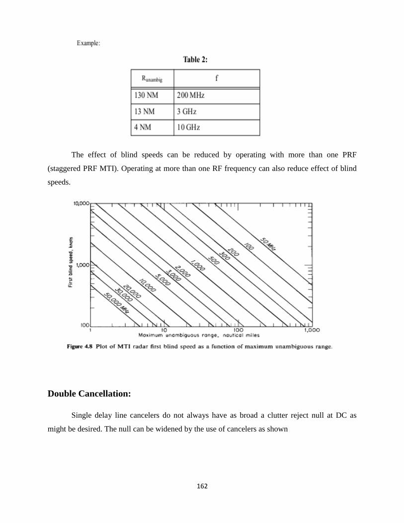
162

The effect of blind speeds can be reduced by operating with more than one PRF

(staggered PRF MTI). Operating at more than one RF frequency can also reduce effect of blind

speeds.

Double Cancellation:

Single delay line cancelers do not always have as broad a clutter reject null at DC as

might be desired. The null can be widened by the use of cancelers as shown

163

In Fig 4.9a, the output of the two single delay line cancellers in cascade is the square of that from

a single delay canceler.

The response of this double delay line canceler is shown in Fig. 4.10.The finite width of the

typical clutter spectrum is also shown to illustrate the additional cancellation offered.

The two delayline canceler of Fig. 4.9b has the same frequencyresponse characteristic as

the double delay line canceler.

Here the output of the adder is Where f(t) is the received video

signal

This arrangement is called a three pulse canceler.

164

Transversal Filters:

The 3 pulse filter of Fig. 4.9b is a transversal filter. The general form is shown below for

N pulses and N-1 delays. It is also called a feed-forward filter, a nonrecursive filter, a finite

memory filter and a tapped delay line filter. The weights for a transversal filter with n delay lines

that gives a sinn(πfdT) are the binomial coefficient with alternating sign

Note: a cascade configuration of three delay lines each connected as a single canceller is called a

triple canceler: but when connected as a transversal filter it is called a four pulse canceler.

165

The transversal filter with alternating binomial weights is closely related to the filter

which maximizes the average of the ratio

Where S/C is the signal to clutter ratio And Ic is the improvement factor for clutter

The average is over the range of Doppler frequencies. Ic is independent of target velocity

and depends onlyon the weights wi, the autocorrelation function (power spectral density) of the

clutter, and the number of pulses.

For the two pulse canceler (single delay line), the optimum weights based on the above

criterion are the same as the binomial weights when the clutter is Gaussian.

For the three pulse canceler, the difference between filter with optimal weights and one

with binomial weights is less than 2 dB.

The difference is small for higher order cancelers also.

For anyorder canceler, the difference between optimum weights and binomial weights is

small over a wide range of clutter spectral widths.

Similarlythe use of a criterion which maximizes the clutter attenuation (Cin/Cout) is also

well approximated by a transversal filter with binomial weights with alternating signs, when the

166

clutter spectrum can be represented by a Gaussian function whose spectral width is small

compared to the PRF. The transversal filter with binomial weights also approximates the filter

which maximizes the Pd for a target at midband Doppler frequency or its harmonics.

The disadvantage is due to notches at DC, the PRF and harmonics of PRF increasing in

width as the number of delay lines increases. The added delay lines reduce the clutter but also

reduce the number of moving targets because of the reduced pass band. For targets uniformly

distributed across the Doppler frequency:

We have for the criterion that -10dB response of the filter is the threshold for detection,

the following table:

Although these filters are optimum for Ic theyare not necessarilybest. They are onlybest

under a given set of assumptions. It would seem that the MTI filter should be shaped to reject the

clutter at DC and around the PRF, but have a flat response over the region where no clutter is

expected.

The transversal filter can be designed to achieve this desirable filter response but needs a

large number of delay lines. This sets a restriction on the radar’s PRF, beamwidth, antenna

rotation rate and dwell time.

Fig 4.12 shows the amplitude response of a 3 pulse canceler with sin2 πfdT(1), a 5 pulse

“optimum” canceler which maximizes Ic (2) and a 15 pulse Chebyshev filter (3). Even a 5 pulse

Chebyshev design gives a significantly wider bandwidth than the 5 pulse optimum design.

Note: the Chebyshev design has a lower Ic but is worthwhile if the clutter spectrum is narrow.

167

When there are onlya few pulses available for processing, there is little that can be done

to control the filter shape. Hence for 3 or 4 pulse cancelers it is best to use the classical sin2 or

sin4 response of the binomial cancelers.

Shaping the Frequency Response:

Non recursive filters employ only feedforward loops. These yield zeroes for synthesizing

the frequency response. If feedback loops are used, each delay line can provide one pole as well

as one zero. The canonical form is shown below:

When feedback loops are used the filter is called recursive. Can synthesize in principle

almost any frequency response using z transform techniques. Canonical configuration is not

always desirable due to delay tolerances.

It has been shown that the canonical configuration can be broken into cascaded sections

with no section having more than two delay elements. This synthesis technique applies to

Chebyshev, Butterworth, Bessel and elliptical filter design.

The recursive delay line filters offer steady state response that is superior to that of

nonrecursive filters. However they have poor transient response due to the feedback loops.

168

The presence of large clutter returns can effectively appear as a large step input which

leads to severe ringing in the filter output which can mask the target signal until the transient

response dies out. In surveillance radar, the number of pulses from anytar get is limited. Hence

the MTI filter is almost always in a transient state for most recursive filters.

A filter with steep frequency response skirts might allow 15 - 30 pulses to be generated at

the filter output due to feedback. This could make the system unusable in situations with large

discrete clutter, or with interference or jamming from other radars. Poor transient response is also

undesirable in radars with step scan phased array, since the e xtra pulses might have to be gated

out after the beam has been moved.

For step scan radars the undesirable transient effects can be overcome by using the initial

return from each new beam position to apply initial conditions to the MTI filter. These initial

conditions are the steady state values that would appear in the filter after an infinitely long

sequence. This effectively suppresses the transient response. An alternative to the recursive filter

is to use multiple PRFs.

169

Multiple (Staggered) PRFs:

Multiple PRFs reduce the effect of blind speeds and also allow a sharper low frequency

cutoff. The blind speeds of two independent radars will be different if their PRFs are different.

This same result can be achieved with one radar which shares its PRFs between 2 or more

values.

PRF can be switched every other scan, every time the antenna is scanned half a beam

width or pulse to pulse (staggered PRF). Fig. 4.16 shows the composite response of MTI with

two separate PRFs with a ratio of 5:4

Note: The first blind speed of the composite is greatly increased (i.e. at fd = 4/T1 = 5/T2). But

regions of low sensitivity appear.

The closer the ratio T1: T2 approaches unity, the greater the frequenc y of the first blind speed,

and the deeper he first null in the vicinity of fd - 1/T1. The null depth can be reduced and the first

blind speed increased by operating with more than 2 PRFs.

Fig 4.17 shows a five pulse stagger (4 periods) response with periods in the ratio 25:30:27:31

Here the first blind speed is 28.25 times that of a constant PRF with the same average period.

If the periods of the staggered pulses have the relationships

Where n1, n2,.....nN are integers

And if vB is the first blind speed of a nonstaggered pulse with period equal to the average period

Then the first blind speed v1 is

Weighting can also be applied to received pulses of a staggered PRF. Fig. 4.18 dashed

curve shows the response of a 5 pulse canceler with fixed PRF and using weights of 7/8;1;-3 3/4;

1 7/8. The solid curve is for a staggered PRF with the same weights but with 4 interpulse periods

of -15%, -5%, 5%, 15%.

170

171

172

Note that the response at the first blind speed is down only 6.6dB. The disadvantage of

staggered PRF is its inabilityto cancel second time around clutter echoes. Such clutter does not

appear at the same range from pulse to pulse and produces uncancelled residue.

Second time around clutter can be removed by the use of constant PRF providing there is

pulse to pulse coherence (i.e. power amplifier form of MTI). Constant PRF might be employed

only over angular sectors where second time around clutter is expected, or by changing the PRF

each time the antenna scans half a beamwidth, or by changing the PRF each scan period.

Range Gated Doppler Filters:

It is possible to use frequency domain band pass filters in MTI radar to sort the Doppler

frequency shifted targets. A narrow band filter with a pass band designed to pass the Doppler

components of a moving target will ring when excited by a short radar pulse.

The narrow band filters means the input pulse since the impulse response is the reciprocal

of the filter bandwidth. This smearing destroys the range resolution.

If there is more than one target in the smeared region they can not be resolved. Even for

one target, noise from other range cells will interfere (collapsing loss) resulting in reduction in

sensitivity. The loss of range information and collapsing loss can be eliminated by quantizing the

range into small intervals (range gating). The width of the range gate is usually of the order of

the pulse width. The range resolution is established by range gating. Once the return is quantized,

the output from each gate is applied to a narrow band filter since the pulse shape need no linger

be preserved for range resolution. Collapsing loss does not take place since noise from other

range intervals is excluded.

The output of the phase detector is sampled sequentially by range gates. The range gate

acts as a switch which opens and closes at the proper time. Gates are activated once each PRI.

The output from a stationary target is s series of pulses of constant amplitude. An echo from a

moving target produces pulses which vary in amplitude according to the Doppler frequency.

The output from the range gates is stretched in boxcar generators (or sample and hold

circuits). This helps the filtering and detection process by emphasizing the fundamental of the

173

modulation frequency and eliminating harmonics of the PRF. Clutter rejection filter is a band

pass filter whose bandwidth depends on the clutter spectrum.

The full wave rectifier then converts the bipolar video to unipolar form. An integrator

acts as a low pass filter. The signal is then applied to the threshold detector circuit.

Following threshold detection the outputs from each range channel must be properly

combined for display on the PPI etc.

The band pass filter can be designed with a variable low frequency cutoff that can be

varied to conform to prevailing clutter conditions (i.e. adaptive).

For example, a wide notch at DC is needed to remove echoes from birds but mayalso

remove some desired targets. Since the appearance of birds varies with time of day and season

the adaptive notch width might be important.

MTI using range gates is more complex than MTI with single delay line canceler. MTI

using range gates improves performance and allows flexibility of range gates and filter

bandwidth.

174

Difference between MTI Radar and CW Radar:

CW Radar MTI Radar

1. Using this radar, we can not measure range

of a target.

1. Using this radar, we can measure range of a

target.

2. This radar can not have blind speeds and

phases.

2. This radar has blind speeds and phases.

3. It is difficult to avoid transmitter to receiver

feed-through.

3. It is easy to avoid transmitter to receiver

feed-through.

4. This radar has little inability to distinguish

between approaching and receiding target.

4. This radar not only distinguishes the

approaching and receiding target but also track

them.

Differences between blind speeds and blind phases:

Blind speeds Blind phases

1.The relative velocities of the target at which

MTI response is zero are called as blind speeds

and are given by

vn is the nth

blind speed

1. The blind phases are due to the presence of

sampling pulses at the same point in the

Doppler cycle at each sampling instant.

2. Due to the presence of blind speeds within a

Doppler frequency band, the capability of radar

may be reduced.

2. When the Doppler frequency is half of the

PRF, blind phases with single has serious

problem, due to which complete signal is lost.

3. By operating with more than one PRF or

operating at more than one RF frequency we

can reduce blind speeds.

3. By using quadrature, we can eliminate the

blind phases.

4. Effect is more in MTI Radars. 4. Effect is more in MTI Radars.

175

Advantages of Time domain Delay-line Canceller over Conventional

Frequency Domain Filter:

1. The delay-line canceller has been widely used in MTI Radar, in order to separating moving

targets from stationary clutter ehile the filter configuration in conventional frequency

domain filter is more complex.

2. The delay-line canceller rejects the DC component of clutter.

3. In time domain delay-line canceller, a single network operates at all frequency ranges, it

does not require a separate fiter for each frequency range.

4. The gain through the delay-line canceller is unity.

5. Delay-line cancellers are used in digital signal processing through which great stability is

achieved.

6. The delay-line canceller serves as an important tool for a MTI designer.

7. The time domain delay-line canceller provides a time delay equal to the pulse repetition

period.

8. The digital processing technology using the delay line cancellers made an introduction of

digital devices for computing the Fourier transform.

Digital Signal Processing:

Allows multiple delay line cancelers with tailored frequency response to be achieved. Is

more dependable, requires less adjustment than analog cancelers, does not vary with temperature

etc. Most advantages of digital MTI result from the use of digital storage in the place of analog

delay lines. Here the IF signals is split into I and Q channels. The outputs of the two phase

detectors are 90˚ out of phase.

The quadrature channel eliminates the effects of blind phases. Note that this is seldom

done in analog delay line cancelers due to the complexity involved with additional analog delay

lines. The baseband bipolar video is sampled at a rate to obtain one or more samples per range

resolution cell. The A/D output is stored in the memory for one PRI and then subtracted from the

words from the next sweep. The I and Q outputs are combined as either

176

. The combined output is then converted to an analog signal with D/A for

display.

Note: more complex filtering schemes are normally implemented.

The memory can be RAM or a shift register. A/D must operate at high speeds to preserve

the information content, and also have sufficient number of bits to quantize the signal to preserve

precision. The number of bits determines the maximum improvement factor for the MTI radar.

The A/D converter must cover the peak excursion of the phase detector output. To ensure this, a

limiter may be necessary. The quantization noise introduced by the A/D imposes a limit to the

improvement factor of

Where 2N - 1 is the number of discrete intervals. This is approximately 6dB / bit

Example: A 9 bit A/D has 511 levels. Thus the maximum resolution is 1 out of 511

177

= 54 dB

Note: IQN = 52.9 which is close

Blind phase - this is different from blind speed. Blind speed occurs when pulse sampling occurs

at the same point on the Doppler cycle at each sampling instant (Fig 4.22a).

Fig. 4.22b shows the I channel with the pulse train such that the signals are of the same

amplitude and with spacing such that when pulse a1 is subtracted from pulse a2 the result is zero.

However a residue is produced when a2 is subtracted from a3, but not when a3 is subtracted from

a4.

Note: The pulse pairs that were lost in the I channel are recovered in the Q channel and vice

versa.

The combination of I and Q channels results in a uniform signal with no loss. An extreme

case, resulting in the complete loss of signal, occurs, with only one channel when the Doppler

frequency is half of the PRF and the phase between the two is such that the echo pulses lie on the

zeroes of the Doppler signal. However if the Q channel is added the all of the echo pulses occur

at the peaks of the Doppler signal. Other phase relationships also give loss with single channel

MTI.

178

Advantages of digital processing over analog delay lines:

1) Greater stability

2) Greater repeatability

3) Greater precision

4) Greater reliability

5) No special temperature control required

6) Greater dynamic range (i.e. no spurious response)

7) Avoids restriction that PRI and delay time must be equal

8) Different PRI can be used (without switching delay lines of various lengths in and out)

9) Greater freedom in selection of amplitude weighting for shaping filters

10) Allows easy implementation of I and Q channels (eliminates blind phases)

Digital Filter Banks and the FFT:

A transversal filter with N outputs (N-1 delays) can be made to form a bank of N

contiguous filters covering the spectrum of 0 to PRF. Consider the transversal filter of Fig. 4.11

to have N-1 delays each with a delay of T = 1/fp. Let the weights at the outputs be

Where i = 1,2,... N represents the ith tap And k = an index from 1 to N-1

Each k value corresponds to a different set of N weights and to a different doppler

frequency response. The N filters generated by the index k constitute the filter bank. The impulse

response of the transversal filter with the above weights is:

The Fourier transform yields the frequency response

The magnitude of the frequency response yields the amplitude characteristic

179

Note that the peak response occurs when the denominator is zero i.e.

π(fT-k/N)= 0,π,2π ....

for k=0, the peak response occurs at f= 0,1/T,2/T etc.

This is a filter centred at DC, the PRF and harmonics of the PRF. This filter has no clutter

rejection capability, b ut it is useful fro pro viding a map of clutter.

The first null occurs when the numerator is 0

For k=0 this is f= 1/NT

The bandwidth between nulls is then 2/NT and the half power bandwidth is: BW(3dB) ≈ 0.9/NT

When k=1, the peak response occurs at f = 1/NT, 1/T + 1/NT....

Hence each k defines a separate filter response, each with a bandwidth between nulls of 2/NT.

180

Since each filter occupies the 1/N bandwidth of a delayline canceler, its SNR will be

greater than the delay line canceler. Also the dividing of the band by N filters allows a measure

of the Doppler frequency to be made. If moving clutter (birds, weather) appears, the threshold of

each filter maybe adjusted individuallyto adapt to the clutter in it. This selectivity allows clutter

to be removed which would be passed by a delay line canceler. The first sidelobe level is at -

13dBc for the filters with the above weights. This can be reduced at the expense of wider

bandwidth by adjusting the weights (windowing).

Two forms of windows are the Hamming and the Hanning.

It is not always convenient to display outputs of all of the Doppler filters. One approach

is to connect filter outputs to a “greatest of” circuit, so that only one output is obtained (Note: the

filter at DC would be excluded).

The improvement factor for each of the 8 filters of a 8 filter bank is shown in Fig. 4.24 as

a function of the standard deviation of the clutter spectrum, for a spectrum represented as a

Gaussian function. For comparison, the improvement factor for an N pulse canceler is shown in

Fig. 4.25

Note: the improvement factor for a two pulse canceler is almost as good as that of the 8 pulse

Doppler filter bank. However, maximizing the improvement factor is not the onlycriterion for

judging the effectiveness of MTI Doppler processes. If a 2 or 3 pulse canceler is cascaded with a

Doppler filter bank, better clutter rejection is obtained.

Fig. 4.26 gives Ic for a 3 pulse canceler cascaded with an 8 pulse filter bank. The upper

figure assumes uniform amplitude weights (-13.2 dB sidelobes) and the lower figure gives the

results for Chebyshev weights (-25 dB sidelobes). It is found that doubling the number of pulses

in the filter bank to 16 does not offer significant improvement (i.e. increased pulses ⇒ increase

in bandwidth as well as decreased sidelobes. If the sidelobes of the individual filters in the filter

bank can be made low, the inclusion of the delay line canceler ahead of it might not be

necessary.

181

Other MTI Delay Lines:

Solid crystal has been mentioned previously.

Electrostatic storage tube

Here the signals are stored on a mesh similar to that of a TV camera. The first sweep

reads the signal on the storage tube. the next sweep written on the same space and

generates the difference between the two. Two tubes are required; one to write and store

the new sweep, the other to subtract the new sweep from the old. The electrostatic storage

tube can be used with different PRFs.

The charge transfer device (CTD) is a sampled data, analog shift register which can be used

as a delayline, transversal filter and recursive filter.

There are two types of CTD:

The bucket brigade device (BBD) with capacitive storage elements separated byswitches.

Here the data is transferred through the BBD at a rate determined bythe rate at which the

Switches are operated. The delay time is determined by the number of stages and the

switching (or clock) speed.

Charge coupled devices (CCDs) are similar except that charge packets are transferred to

adjacent potential wells by a clocked potential gradient

Notes: The sampling frequency must give one or two samples per resolution cell. No A/D or

D/A required as for digital systems.

MTI cancelling can be done at IF. Here no blind phases occur. Finally the video can FM

modulate a carrier f or acoustic delay. This avoids problems of amplitude stability of acoustic

delay lines.

182

183

184

Example of an MTI Radar Processor:

The moving target detector (MTD) was developed byLincoln Labs for the FAA’s airport

surveillance radars (ASR). The ASR is medium range (60 NM) radar located at most US

airports. It has 2.7 to 2.9 GHz RF, 1μs pulse width, 1.4 ˚ azimuth beamwidth, antenna rotation

rate of 12.5 to 15 RPM PRF from 700 to 1200 Hz and average power from 400 to 600 W.

The MTD processor is based on digital technology. Uses a 3 pulse canceler followed by

an 8 pulse FFT Doppler filter bank with weighting to reduce sidelobes. The total system has

alternating PRFs to eliminate blind speeds, adaptive thresholds and a clutter map used for

detecting targets with zero radial speed.

The measured Ic of the MTD on the ASR was 45 dB (20 dB better than with a

conventional 3 pulse MTI processor). The MTD also achieves a narrower notch at zero velocity

blind speeds. The processor is preceded by a large dynamic range receiver to avoid reduction in

Ic caused by limiting.

The IF is applied to I & Q detectors and the video is A/Dd with 10 bit resolution. The

range totalling 47.5 NM is divided into 1/16 NM intervals and the azimuth into 0.75 ˚ intervals.

In each 0.75˚ interval (≈ 1/2 beamwidth) 10 pulses are transmitted at constant PRF.

On receive the 10 pulses are processed by the delay line canceller and Doppler filter bank

which forms 8 Doppler filters. Hence the radar output is divided into 2,920,000

range/azimuth/doppler cells. Each cell has its own adaptive threshold. In the alternate 0.75˚

azimuth intervals another 10 pulses are transmitted at a different PRF. Changing PRF every 10

pulses eliminates second time around clutter. The MTD processor is shown in Fig. 4.27. The 3

pulse canceler ahead of the filter bank eliminates stationary clutter ahead of the filter bank and

reduces the dynamic range required of the Doppler filter bank.

Since the first two pulses of a three pulse canceler are useless, only the last 8 of the 10

pulses are passed to the filter bank (implemented using the FFT).

Following the filter bank, weighting is applied in the frequencydomain to reduce the filter

sidelobes. This is necessary since the frequency spectrum of rain and wind blown clutter requires

sidelobes lower than the -13.2 dB available from uniformly weighted samples.

185

The magnitude operation forms

Separate thresholds are applied to each filter. For non zero velocityresolution cells the

thresholds are established byscanning the detected outputs of the same velocityfilter in 16 range

cells, eight on either side of the cell of interest. Hence each filter output is averaged over one

mile in range to get the mean level of non zero velocityclutter.

The filter thresholds are determined by multiplying the mean levels by a constant to

achieve the desired Pfa. This adaptive threshold on each doppler filter at each range cell provides

a constant false alarm rate (CFAR) and results in subclutter visibility (for different radial

velocities of aircraft and weather). A digital clutter map establishes the thresholds for zero

velocity cells. The map is implemented with one word for each of the 365000 range/azimuth

cells. The purpose of the zero velocity filters is to recover the clutter signal and use it to establish

a threshold for targets with zero radial velocity.

In each cell of the ground clutter map is stored the average value of the output of the zero

velocityfilter for the past 8 scans (32 seconds) On each scan 1/8 of the output is added to 7/8 of

the value stored in the map. The map is built up recursively requiring 10 to 20 scans to establish

steady state clutter values.

186

The values in the map are multiplied by a constant to establish a threshold for zero

velocity targets. This allows elimination of usual MTI blind speed at zero relative velocity for

targets with large cross section. The MTD filters are shown in Fig. 4.28.

Here the filters 3 through 7 establish the threshold from the mean signal in 16 range cells.

Filter 1 establishes the threshold from the clutter map. Filters 2 and 8 adjacent to the zero

velocity filter establish the threshold from the larger of the mean signal over 16 range cells and

the clutter map.

Fig 4.28 also shows the advantage of using 2 PRFs to detect targets in rain. As shown, the

PRFs are 20% different. Typical rain storm spectrum is shown o the bottom and has about 25 to

30 knots width centred any where from - 60 to +60 knots.

An aircraft return is also shown at the right of the figure and is shown as occupying filters

6 and 7 on PRF-1 and filters 7 and 8 on PRF-2 (the difference is due to frequency foldover).

With PRF-2 the aircraft velocity is competing with the rain clutter, but at PRF-1 it is clear of

187

clutter. Hence by using 2 PRFs alternating every 10 pulses, aircraft targets will appear in at least

one filter free of rain (except when the aircraft’s radial velocity is that of the rain).

Interference from other radars may appear as one large return among the ten returns

processed. The MTD has an interference eliminator which compares the magnitude of each of

the ten pulses against the average magnitude of the ten pulses. If anypulse is greater than 5 times

the average, all information from that range/azimuth cell is discarded. The output of the MTD is

a hit report containing azimuth, range, amplitude, filter number and PRF.

On one scan, a large aircraft might be reported from more than one doppler filter, from

several coherent processing intervals and from adjacent range cells. Up to 20 hit reports might be

generated from a single large target.

A post processor groups together all reports which appear to originate from the same

target and interpolates to find the best azimuth, range, and amplitude and radar velocity. Target

amplitude and Doppler are used to eliminate small cross section and low speed angle echoes

before targets are delivered to the automatic tracking circuits.Tracking circuits eliminate false hit

reports which do not form logical tracks. The output of the automatic tracker is what is displayed

on the PPI.

Since the MTD processor eliminates large amounts of clutter and has a low false

detection rate, its output can be remoted via narrow bandwidth telephone.

Limitations of MTI Performance:

Improvement in signal to clutter is affected by factors other than the Doppler spectrum.

Instabilities in the transmitter and receiver, physical motion of the clutter, finite time on target

and receiver limiting all affect Ic.

Definitions:

1) MTI Improvement Factor I: The signal to clutter ratio at the output of the MTI

system divided by the signal to clutter ratio at the input, averaged over all of the target radial

velocities of interest.

188

2) Subclutter Visibility (SCV): The ratio by which the target echo may be weaker

than the coincident clutter echo power and still be detected with specified Pd and Pfa. All

target radial velocities are assumed equally likely

Note: A typical value is 30 dB

Note: Two radars with the same subclutter visibility might not have the same ability to detect

targets in clutter if the resolution cell of one is greater and accepts more clutter echo power

3) Clutter Visibility Factor Voc: The signal to clutter ratio after cancellation (or

Doppler processing) that provides the stated Pd and Pfa.

4) Clutter Attenuation CA: the ratio of the clutter power at the canceler input

to the clutter residue at the output, normalized (divided by) to the attenuation of a single

pulse passing through the unprocessed channel of the canceler

5) Cancellation Ratio: The ratio of canceler voltage amplification fro fixed target

echoes received with a fixed antenna, to the gain for a single pulse passing through the

unprocessed channel of the canceler.

Note:

Note: When the MTI is limited by noise like system instabilities, Voc should be chosen as the

SNR for range equation calculations.

Note: when the MTI is limited by antenna scanning fluctuations, let Voc = 6dB for a single

pulse.

Note: Once again, I is the preferred measure of MTI performance but does not account for

possible poor performance at certain velocities

6) Interclutter Visibility: The ability of the MTI to detect moving targets in

clear resolution cells between patches of strong clutter. Resolution cells can be range,

azimuth or Doppler.

Note: the higher the radar resolution, the better the interclutter visibility. A medium resolution

radar with 2μs pulse width and 1.5 ˚ beamwidth has sufficient resolution to achieve a 20 dB

advantage over low resolution radars

189

7) Equipment Instabilities: The apparent frequency spectrum from perfectly

stationary clutter can be broadened (and hence will degrade the MTI improvement factor)

due to the following:

Pulse to pulse changes in amplitude

Pulse to pulse changes in frequency

Pulse to pulse changes in phase

Timing jitter on transient pulse

Variations in time delay through the delay lines

Changes in pulse width

Changes in coho or stalo between time of transmit and time of receive

8) Consider the effect of phase variations

Let the echo from a stationary clutter on pulse 1 and pulse 2 be

Where Δφ is the change in oscillator phase between the two

pulses

9) On subtraction

Hence the limitation on the improvement factor due to oscillator instability is

Note: To achieve I > 40 dB requires Δφ < 0.01 rad from pulse to pulse!. This applies to the coho

locking or the phase change introduced by the HPA.

The limits to I imposed by pulse to pulse instability are:

190

Note: the digital processor does not experience degradation due to timing jitter of the transmit

pulse if the clock controlling the processor timing is started from the detected RF envelope of the

transmitted pulse.

10) Internal Fluctuation of Clutter: Absolutely stationary clutter - buildings,

water towers, mountains, bare hills

Dynamic clutter - trees, vegetation, sea, rain, chaff

Can limit the performance of MTI

Most fluctuating clutter targets can be represented by a model consisting of many

independent scatterers located in the resolution cell.

Any motion of the scatterers relative to the radar results in a different vector sum from

pulse to pulse. Fig. 4.29 shows the power spectral density of clutter for a 1 GHz carrier.

191

Experimentally measured spectra of clutter can be approximated by

Where W(f) = clutter power spectrum

g(f) = Fourier transform of the clutter waveform

f0 = radar carrier frequency and a = a parameter (given by Fig 4.29)

This equation can be rewritten as:

Where σc is the RMS clutter frequency spread in Hz

or as

Where σv is the clutter velocity spread in m/s

Note:

192

The improvement factor can be written as

Where CA = Ci/C0 - clutter attenuation averaged over all doppler frequencies

For a single delay line canceler

Where H(f) is the frequency response of the canceler

For a single delay line canceler, h(f) = 1- exp(-j2πfT)

= 2jsin(πfT) exp(-jπfT)

Therefore,

Assuming σc << 1/T yields,

If the exponential is small, we can use the first two terms of its series expansion

193

Now the average gain (S0/Si)avg for the single delay line canceler is 2

Hence,

Similarly for a double canceler, whose average gain is 6,

A plot of above equation is shown in Fig 4.30 with fpλ as a parameter. Several representative

examples of clutter are indicated at particular values of σv.

Note: σv (spectral spread in velocity) is with respect to the mean velocity which for ground

clutter is zero.

Rain, sea echo and chaff have non zero mean velocity which must be accounted for

Note: the frequency dependence of equations 25 and 26 for the clutter spectrum can not be

extended over too great a frequencyrange since no account is taken of variation of cross section

of individual scatterers as a function of frequency.

For example the leaves and branches of trees have considerably different reflecting

properties at Ka band where their dimensions are comparable to λ, than at UHF frequencies.

The general form for an N pulse canceler with Nl = N-1 delay lines is

194

Antenna Scanning Modulation:

A scanning antenna observes a target for time t0

Where nB is the number of hits received

The received pulse train of finite duration t0 has a frequency spectrum which is

proportional to. Hence even if the clutter were perfectly stationary, the clutter spectrum would

have a finite width due to the finite time on target.

If the clutter spectrum is too wide due to too short an observation interval, the

improvement factor will be affected. This limitation is called scanning fluctuation or scanning

modulation.

To find the limitation on Ic we first find the clutter attenuation CA

195

Here WS(f) describes the spectrum produced by the finite time on

target and H(f) is the MTI processor frequency response.

If the antenna main beam is approximated bya Gaussian shape, the spectrum will also be

Gaussian. Hence the results previously derived for a Gaussian clutter spectrum can be applied.

Thus equations I1c and I2c apply for the antenna scanning fluctuations with the correct

interpretation of σc (the RMS spread of the spectrum about the mean).

Here the voltage waveform for the clutter is modulated bythe antenna power pattern (equal to the

two way field strength pattern), as it is rotated

Now, Where θ and θB are in degrees

Therefore

Where Sa(t) is the modulation of the received signal due to the

antenna pattern and is the scan rate in ˚/s.

The spectrum is found by taking the Fourier transform

Since this is a Gaussian function we must have

196

Hence,

Note: This is for the voltage spectrum

For the power spectrum we have,

Hence the σs due to the antenna scanning is

Substituting this for σc , we get,

Note: the stepped scan antenna also is limited in MTI performance by the finite time on target.

The time waveform is rectangular which gives a different improvement factor.

197

Limiting in MTI Radar:

A limiter is used just before the MTI processor to prevent the residue from large clutter

echoes from saturating the display. Ideally an MTI radar should reduce clutter to a level

comparable to noise. However, when I is not great enough, the clutter residue will appear on the

displayand prevent the detection of aircraft whose radar cross section is larger than the clutter

residue. This condition can be prevented bysetting the limit L relative to the noise N equal to the

MTI improvement factor I.

If the limit le vel is set too high, clutter residue obscures part of the display. If the limit is

set too lo w, there may be a black hole effect. The limiter provides a CFAR (Constant False

Alarm Rate). A nonlinear limiter however causes the spectrum of strong clutter to spread into

the canceler pass band and results in the generation of additional residue which degrades the

MTI performance.

Figure 4.32 plots I for 2 pulse and 3 pulse cancelers with various levels of limiting. The

abscissa applies to Gaussian clutter spectrum generated by clutter motion (σv) or by antenna

scanning modulation (nB). Here C/L is the ratio of RMS clutter power to the IF limit level.

Note: The loss of I increases with the complexity of the canceler. Limiting in a 3 pulse canceler

will cause a 15 to 25 dB reduction in performance. A 4 pulse canceler with limiting is only 2 dB

better than a 3 pulse canceler. Hence adding complexity is not justified in a limiting environment

Limiting is not needed if processor I is large enough to reduce the largest clutter to the

noise level (typically requires I ≈ 60 dB). This is difficult to achieve since it requires the receiver

to have a linear dynamic range of at least 60 dB, the A/D must have at least 11 bits, the

equipment must be stable, the processor must be designed for I = 60 dB and the number of pulses

processed must be sufficient to reduce the antenna scanning modulation.

198

199

Tracking with Surveillance Radar:

The track of a target can be determined with surveillance radar from the coordinates of

the target measured from scan to scan. The quality of such a track depends on the time between

observations, the location accuracy of each observation and the number of extraneous targets

present in the vicinity of the tracked target.

A surveillance radar which develops tracks on targets it has detected is called a “track

while scan” (TWS) radar. Tracks can be obtained by having an operator mark the location of a

target on the face of the PPI with a grease pencil on each scan.

A single operator however can not handle more than about 6 target tracks when the radar

has a twelve second scan rate. Also an operator’s effectiveness in detecting new targets decreases

rapidly after 1/2 hour of operation. These problems are avoided by automating the target

detection and tracking process. This is called automatic detection and tracking (ADT)

The ADT performs the following functions:

Target detection

Track initiation

Track association

Track update

Track smoothing

Track termination

The automatic detection quantizes the range into intervals equal to the range resolution.

At each range interval the detector integrates n pulses (n is the expected number of hits expected

from the target due to the antenna scan rate). The integrated pulses are compared with the

threshold to determine the presence or absence of a target.

An example is the “moving window detector” which examines continuouslythe last n

samples within each quantized range and announces the presence of a target if m out of n of

these samples crosses a preset threshold. By locating the centre of the n pulses, an estimate of the

target’s angular direction can be obtained. This is called “beam splitting”.

200

If there is only one target present within the radar’s coverage, then the detection on two

scans is all that is required to establish a tar get track and estimate its’ v elocity. However there

are usuallyother targets plus clutter echoes and hence three or more detections are necessary to

establish a track reliably without the generation of false tracks.

A computer can recognize and reject false tracks, however too many false tracks can

overload a computer. Hence the radar using ADT should exclude unwanted signals from clutter

and interference. A good ADT system therefore requires a good MTI and a good CFAR receiver.

A clutter map generated by the radar is sometimes used to reduce the load on the tracking

computer by blanking the clutter areas and removing detections associated with large point

clutter sources not rejected by the MTI. Slowly moving echoes that are not of interest can also be

removed by the clutter map.

The availability of distinctive target characteristics such as altitude might prove of help

when performing track association. When a new detection is received, an attempt is made to

associate it with existing tracks. This is aided byestablishing for each track a small search region

(gate) within which a new detection is predicted based on the estimate of the target speed and

direction. It is desired to make the gate as small as possible to avoid having more than one echo

fall within it when traffic density is high, or when two tracks are close. However a large gate is

required if the tracker is to follow target maneuvres. Hence more than one gate size may be used.

The size of the gate depends on the accuracy of the track. When a target does not appear

in the small gate, a larger gate could be used. The size of the second gate would depend on the

maximum acceleration expected of the target. On the basis of past detections, the track while

scan radar must make smoothed estimates of the target position and velocity as well as the

predicted position and velocity.

One method of computing this information is the α−β tracker (also called the g-h tracker).

Here the present smoothed target position and velocivty are computed using

Where xpn = the predicted position of the target at the nth scan

xn = the measured position at the nth scan

201

α = the position smoothing parameter

β = the velocity smoothing parameter

Ts = the time between observations

The predicted position at the n+1 scan is

When acceleration is important, a third equation can be added to describe an α−β−γ

tracker where γ is the acceleration smoothing parameter.

If α = β = 0 then the tracker uses no current data, only smoothed data.

If α = β = 1 then no smoothing is included at all

The α−β filter is designed to minimize the mean square error in the smoothed (filtered)

position and velocity assuming small velocity changes between observations. To minimize the

output noise variance at steady state and the transient response to a maneuvering target modeled

by a ramp function the α−β coefficients are related by

The choice of α between 0 and 1 depends on the system application and in particular on

the tracking bandwidth.

A compromise must be made between good smoothing (narrow bandwidth) and rapid

response to maneuver (wide bandwidth).

A criterion for selecting the α,β coefficients is based on the best linear track fitted to the

radar data in the least squares sense. This gives values

Where n = the number of scans or target observations

202

A standard α − β tracker does not handle the maneuvering target. An adaptive α − β

tracker is one which varies the two smoothing parameters to achieve a variable bandwidth so as

to be able to follow maneuvres.

The value of α can be set by observing the measurement error xn - xpn. At the start of the

tracking, the bandwidth is set to be wide and is narrowed down if the target moves in a straight

line. As the target maneuvres, the bandwidth is widened to keep the tracking error small.

A Kalman filter is similar to an adaptive α − β tracker except that it inherently provides

for dynamical targets. Here a model for the measurement error has to be assumed, as well a

model of the target trajectoryand the disturbance of the trajectory.

Disturbances might be due to neglect of higher order derivatives in the model of the

dynamics, random motions due to atmospheric turbulence, and target maneuvres.

Kalman filters can use a wide varietyof models for measurement noise and

trajectorydisturbance, however these are usually assumed to be white noise with zero mean.

A maneuvering target does not always fit this model since it produces correlated

observations. Proper inclusion of realistic dynamical models increases the complexity of the

calculations.

The Kalman filter is sophisticated but costly to implement. Its chief advantage over the

classical α − β tracker is its inherent ability to account for maneuvre statistics. If Kalman filters

were restricted to modelling the target trajectoryas a straight line and if the measurement noise

and trajectory disturbance noise were modeled as white Gaussian noise with zero mean, then the

Kalman filter equations reduce to α − β tracker equations, with the α and β computed

sequentially by the Kalman filter procedure.

The classical α − β is easy to implement. To handle maneuvering targets, some means

maybe included to detect maneuvres and to change the values of α and β. The data rate might

also be increased during target maneuvres in some radar systems. As means for choosing α and β

become more sophisticated, the optimal α − β tracker becomes equivalent to a Kalman filter even

for a target trajectory with error. Here the computation of α and β require a knowledge of the

statistics of the measurement errors and the prediction errors, and are determined in a recursive

203

manner in that theydepend on previous estimates of the mean square error in the smoothed

position and velocity.

Note: The concept of the α − β tracker or the Kalman filter apply also to a continuous single

target tracker where the error signal is processed digitally. The equations describing the α − β

tracker are equivalent to a Type II servo system

Of the track while scan radar does not receive target information on a particular scan, the

smoothing and predicting operations can be continued by accounting for the missing data. When

data to update a track is missing for a sufficient number of consecutive scans, the track is

terminated.

Example: if the criterion for establishing a track is 3 target reports, 5 consecutive misses is

suitable for termination.

ADT effectively reduces the bandwidth in the radar output allowing the data to be

transmitted to a remote site via narrow band phone lines. This allows the outputs from several

radars to be communicated to a central control point economically.

The adaptive thresholding of the automatic detector can cause worsening of the range

resolution. It would seem that two targets might be resolved if their separation is about 0.8 pulse

width. However with automatic detection, the probabilityof resolving targets in range onlye

xceeds 0.9 if theyare separated by 2.5 pulse widths.

To achieve this resolution, a log video receiver should be used and the threshold should

be proportioned to the smaller of the two means calculated from a number of reference cells on

either side of the test cell. This resolution limit assumes that the shape of the return pulse is not

known. (If it were, it would be possible to resolve targets within one pulse width).

When more than one radar are covering the same volume of space, it is sometimes

desirable to combine their outputs to form a single track file (Automatic Detection and Integrated

Tracking, ADIT). ADIT has the advantage of a greater data rate than a single radar and reduces

the likelihood of a loss of target detections caused by antenna lobing, fading, interference and

clutter. The integrated processing allows a favourable weighting of better data and lesser

weighting of the poorer data.

204

OBJECTIVE TYPE QUESTIONS

1. Radar range primarily depends upon [ ]

a. peak transmitted power b. average transmitted power

c. independent of transmitted power d. resolution of radar

2. In radar system which of the following is used for transmitter output tubes [ ]

a. parameter amplifier b. RC coupled amplifier

c. klystron only d. magnetron or travelling wave tube

3. A radar is to have maximum range of 60km. The maximum allowable pulse repetition

frequency for unambiguous reception should be [ ]

a. 25 pps b. 250 pps c. 2500 pps d. 25,000 pps

4. An MTI radar operates at 10 GHz with PRF of 3000pps. The lowest blind speed will be

90km/hr

a. 40 km/hr b. 66 km./hr c. 81 km/hr d. 162 km/hr

5. In which of the following case the lowest blind speed will be 90 km/hr [ ]

a. frequency 1 GHz an PRF 300 pps b. frequency 3 GHz and PRF 500 pps

c. frequency 5 GHz and PRF 700 pps d. frequency 7 GHz and PRF 1000 pps

6. If a given maximum range of radar is to be doubled, all other factors remaining constant the

peak power must be increased [ ]

a. four fold b. eight fold c. sixteen fold d. thirty fold

7. The maximum range of a radar depends on all of the following except [ ]

a. peak transmitted pulse power b. direction of movement of target

c. target area d. capture are

8. The antenna used for radar is [09M03] [ ]

205

a. paraboloidal antenna b. isotropic radiator

c. resonant antenna d. whip antenna

9. Noise figure of radar receiver is 12 dB and its bandwidth is 2.5 MHz. the value of

Pmin for this radar will be [ ]

a. 1.59 X 10 -9

watt b. 1.59 X 10-13

watt c. 1.59 X 10-15

watt d. 1.59 X 10-17

watt

10. IN radar system the lobe switching technique is used to [09S01] [ ]

a. scan the area b. move antenna in the direction fo the object

c. locate the target accurately d. move the weapon in the required direction

11. Radar display is [ ]

a. A scope display `b. PPI c. MTI d. CRO

12. The minimum receivable signal in radar receiver which has an IF bandwidth of 1.5

MHz and is 9 dB noise figure will be [ ]

a. 4.17 X 10 -10 watt b. 4.17 X 10 -12 watt

c. 4.17 X 10-14 watt d. 4.17 X 10-16 watt

13. The advance and retard switches for the bearing circuit are needed due to [ ]

a. the gate generators being unstable b. scanner and deflection coil misalignment

c. in accuracies in the power supply d. failure of the switch circuits

14. When real transmitted power on a radar system, is increased by a factor of 16,. The

maximum range will be increased by a factor of [ ]

a. 2 b. 4 c. 8 d. 16

15. The signal arriving from the transmitter to the display unit is the [ ]

a. trigger b. echoes c. heading marker d.bearing information

206

16. The delay unit section of the VRM/ delay unit can be used to [ ]

a. extend the range of radar` b. reduce radar interference

c. expand an area for examination

d. extend the range of radar and expand an area for examination

17. The trigger circuit [ ]

a. is a switch connecting high voltage through to magnetron

b. is a master timing device of the radar

c. is microwave frequency oscillator

d. receives bearing information from the scanner.]

18. An AFC system produces a control voltage to control the --- frequency [ ]

a. Magnetrons b. Local oscillator’s

c. PRF oscillator’s d. Tabulator

19. The local oscillator’s frequency is [ ]

a. 60 MHz above the echo frequency b. 60 MHz below the echo frequency

c. 30 MHz above the echo frequency d. 30 MHz below the echo frequency

20Sea clutter returns occur [10M05] [ ]

a. due to reflections from rain clouds b. at short ranges

c. due to land reflections d. due to satellite reflections

Answers:

1.a 2.d 3.c 4.d 5.b 6.c 7.b 8.a 9.b 10.c

11.a 12.c 13.b 14.a 15.a 16.d 17.b 18.b 19.b 20.b

207

ESSAY TYPE QUESTIONS

1. What is a delay line canceller? Illustrate the concept of blind speeds based on the frequency

response of a single delay line canceller.

2. Discuss the factors limiting the performance of an MTI system.

3. What are blind speeds? Suggest a method to reduce the effect of blind speeds for

unambiguous detection of a moving target.

4. Calculate the lowest blind speed of an MTI system operating at 3.6 cm wave length and

transmitting at a pulse repetition time of 330 µS.

5. Explore the possibility of broadening the clutter rejection null using a second dlay line

canceller in the MTI radar system.

6. Describe automatic tracking of a target through range gating technique for unambiguous

detection of a moving target.

7. Calculate the lowest blind speed of an MTI system operating at 4.2 cm wave length and

transmitting at a pulse repetition time of 286 µS.

8. Explore the possibility of broadening the clutter rejection null using a second delay line

canceller in the MTI radar system.

9. With the help of necessary blo ck diagram explain the operation of an MTI radar system

with a power amplifier in the transmitter.

10. Compare and contrast the situations with a power amplifier and a power oscillator in the

transmitter of an MTI system

11. Describe the method of staggering pulse repetition frequency to reduce the effect of blind

speeds in an MTI system.

12. Explain the following limitations of MTI radar.

(a) Equipment instabilities.

(b) Scanning modulation.

(c) Internal fluctuation of clutter.

208

13. MTI radar is operated at 9GHz with a PRF of 3000 pps. Calculate the first two lowest

blind speeds for this radar. Derive the formula used.

14. Discuss the liminations of non-cohorent MTI Radar systems.

15. Write the description of Range gate Doppler filters.

16. Explain the operation of MTI radar with 2 pulse repetition frequencies.

17. Explain the function of time domain filter with an example.

18. MTI radar operates at 10GHz with a PRF of 300 pps. Calculate the lowest blind speed?

209

UNIT-VI

TRACKING

RADAR

210

Explain tracking principles:

A tracking-radar system

(1) Measures the coordinates of a target and

(2) Provides data which may be used to determine the target path and to predict its future

position.

All or only part of the available radar data-range, elevation angle, azimuth angle, and

Doppler frequency shift may be used in predicting future position; that is, radar might track in

range, in angle, in doppler, or with any combination. Almost any radar can be considered

tracking radar provided its output information is processed properly. But, in general, it is the

method by which angle tracking is accomplished that distinguishes what is normal normally

considered tracking radar from any other radar. It is also necessary to distinguish between

continuous tracking radar and a track-while-scan (TWS) radar.

The continuous tracking radar supplies continuous tracking data on a particular target,

while the track-while-scan supplies sampled data on one or more targets. In general, the

continuous tracking radar and the TWS radar employ different types of equipment.

The antenna beam in the continuous tracking radar is positioned in angle by a

servomechanism actuated by an error signal. The various methods for generating the error signal

may be classified as sequential lobing, conical scan, and simultaneous lobing or monopulse. The

range and Doppler frequency shift can also be continuously tracked, if desired, by a servocontrol

loop actuated by an error signal generated in the radar receiver.

Explain sequential lobing:

The antenna pattern commonly employed with tracking radars is the symmetrical pencil

beam in which the elevation and azimuth beamwidths are approximately equal. However, a

simple pencil-beam antenna is not suitable for tracking radars unless means are provided for

determining the magnitude and direction of the target's angular position with respect to some

reference direction, usually the axis of the antenna. The difference between the target position

and the reference direction is the angular error. The tracking radar attempts to position the

antenna to make the angular error zero. When the angular error is zero, the target is located along

the reference direction.

One method of obtaining the direction and the magnitude of the angular error in one

coordinate is by alternately switching the antenna beam between two positions (Fig.). This is

211

called lobe switching, sequential switching, or sequential lobing. Fig (a) is a polar representation

of the antenna beam (minus the sidelobes) in the two switched positions. A plot in rectangular

coordinates is shown in Fig (b), and the error signal obtained from a target not on the switching

axis (reference direction) is shown in Fig (c).

The difference in amplitude between the voltages obtained in the two switched positions

is a measure of the angular displacement of the target from the switching axis. The sign of the

difference determines the direction the antenna must be moved in order to align the switching

axis with the direction of the target. When the voltages in the two switched positions are equal,

the target is on axis and, its position may be determined from the axis direction.

Fig: Lobe-switching antenna patterns and error signal (one dimension). (a) Polar representation

of switched antenna patterns (b) rectangular representation (c) error signal.

Two additional switching positions are needed to obtain the angular error in the

orthogonal coordinate. Thus a two-dimensional sequentially lobing radar might consist of a

cluster of four feed horns illuminating a single antenna, arranged so that the right-left, up-down

212

sectors are covered by successive antenna positions. Both transmission and reception are

accomplished at each position. A cluster of five feeds might also be employed, with the central

feed used for transmission while the outer four feeds are used for receiving. High-power RF

switches are not needed since only the receiving beams, and not the transmitting beam, are

stepped in this five-feed arrangement.

One of the limitations of a simple unswitched nonscanning pencil-beam antenna is that

the angle accuracy can be no better than the size of the antenna beamwidth. An important feature

of sequential lobing (as well as the other tracking techniques to be discussed) is that the

targetposition accuracy can be far better than that given by the antenna beamwidth. The accuracy

depends on how well equality of the signals in the switched positions can be determined. The

fundamental limitation to accuracy is system noise caused either by mechanical or electrical

fluctuations.

Sequential lobing, or lobe switching, was one of the first tracking-radar techniques to be

employed. Early applications were in airborne-interception radar, where it provided directional

information for homing on a target, and in ground-based antiaircraft fire-control radars. It is not

used as often in modern tracking-radar applications.

Explain conical scanning method:

The logical extension of the sequential lobing technique is to rotate continuously an

offset antenna beam rather than discontinuously step the beam between four discrete positions.

This is known as conical scanning (Fig). The angle between the axis of rotation (which is

usually, but not always, the axis of the antenna reflector) and the axis of the antenna beam is

called the squint angle.

Consider a target at position A. The echo signal will be modulated at a frequency equal to

the rotation frequency of the beam. The amplitude of the echo-signal modulation will depend

upon the shape of the antenna pattern, the squint angle and the angle between the target line of

sight and the rotation axis. The phase of the modulation depends on the angle between the target

and the rotation axis. The conical scan modulation is extracted from the echo signal and applied

to a servo-control system which continually positions the antenna on the target. When the

antenna is on target, as in B of Fig, the line of sight to the target and the rotation axis coincide,

and the conical-scan modulation is zero.

213

Fig: Conical-scan tracking

A block diagram of the angle-tracking portion of typical conical-scan tracking radar is shown in

Fig. The antenna is mounted so that it can be positioned in both azimuth and elevation by

separate motors, which might be either electric- or hydraulic-driven. The antenna beam is offset

by tilting either the feed or the reflector with respect to one another.

Fig: Block diagram of conical-scan tracking radar

One of the simplest conical-scan antennas is a parabola with an offset rear feed rotated

about the axis of the reflector. If the feed maintains the plane of polarization fixed as it rotates, it

is called a nutating feed. A rotating feed causes the polarization to rotate. The latter type of feed

requires a rotary joint. The nutating feed requires a flexible joint. If the antenna is small, it may

214

be easier to rotate the dish, which is offset, rather than the feed, thus avoiding the problem of a

rotary or flexible RF joint in the feed.

A typical conical-scan rotation speed might be 30 r/s. The same motor that provides the

conical-scan rotation of the antenna beam also drives a two phase reference generator with two

outputs 90° apart in phase. These two outputs serve as a reference to extract the elevation and

azimuth errors. The received echo signal is fed to the receiver from the antenna via two rotary

joints (not shown in the block diagram). One rotary joint permits motion in azimuth, the other, in

elevation.

The receiver is a conventional superheterodyne except for features peculiar to the conical

scan tracking radar. One feature not found in other radar receivers is a means of extracting the

conical-scan modulation, or error signal. This is accomplished after the second detector in the

video portion of the receiver.

The error signal is compared with the elevation and azimuth reference signals in the

angle-error detectors, which are phase-sensitive detectors. A phasesensitive detector is a

nonlinear device in which the input signal (in this case the angle-error signal) is mixed with the

reference signal. The input and reference signals are of the same frequency. The output d-c

voltage reverses polarity as the phase of the input signal changes through 180°.

The magnitude of the d-c output from the angle-error detector is proportional to the error,

and the sign (polarity) is an indication of the direction of the error. The angle-errordetector

outputs are amplified and drive the antenna elevation and azimuth servo motors.

The angular position of the target may be determined from the elevation and azimuth o

the antenna axis. The position can be read out by means of standard angle transducers such as

synchros, potentiometers, or analog-to-digital-data converters.

Explain the block diagram of the AGC portion of tracking radar receiver:

The echo-signal amplitude at the tracking-radar receiver will not be constant but will vary

with time. The three major causes of variation in amplitude are (1) the inverse-fourth-power

relationship between the echo signal and range, (2) the conical- scan modulation (angle-error

signal), and (3) amplitude fluctuations in the target cross section.

The function of the automatic gain control (AGC) is to maintain the d-c level of the

receiver output constant and to smooth or eliminate as much of the noise like amplitude

215

fluctuations as possible without disturbing the extraction of the desired error signal at the

conical-scan frequency.

One of the purposes of AGC in any receiver is to prevent saturation by large signals. The

scanning modulation and the error signal would he lost if the receiver were to saturate. In the

conical-scan tracking radar an AGC that maintains the d-c level constant results in an error signal

that is a true indication of the angular pointing error. The d-c level of the receiver must be

maintained constant if the angular error is to be linearly related to the angle-error signal voltage.

An example of the AGC portion of a tracking-radar receiver is shown in Fig. 6.4. A

portion of the video-amplifier output is passed through a low-pass or smoothing filter and fed

back to control the gain of the IF amplifier. The larger the video output, the larger will be the

feedback signal and the greater will be the gain reduction.

The filter in the AGC loop should pass all frequencies from direct current to just below

the conical-scan-modulation frequency. The loop gain of the AGC filter measured at the conical-

scan frequency should be low so that the error signal will not be affected by AGC action.

Fig: Block diagram of the AGC portion of a tracking-radar receiver

The output of the feedback loop will be zero unless the feedback voltage exceeds a

prespecified minimum value Vc. In the block diagram the feedback voltage and the voltage Vc

are compared in the d-c amplifier. If the feedback voltage exceeds Vc, the AGC is operative,

while if it is less, there is no AGC action. The voltage Vc is called the delay voltage. The purpose

of the delay voltage is to provide a reference for the constant output signal and permit receiver

gain for weak signals. If the delay voltage were zero, any output which might appear from the

receiver would be due to the failure of the AGC circuit to regulate completely.

In many applications of AGC the delay voltage is actually zero. This is called undelayed

AGC. In such cases the AGC can still perform satisfactorily since the loop gain is usually low for

216

small signals. Thus the AGC will not regulate weak signals. The effect is similar to having a

delay voltage, but the performance will not be as good.

Explain the Block diagram of amplitude-comparison monopulse radar for

single angular coordinate and explain its operation:

The amplitude-comparison monopulse employs two overlapping antenna patterns (Fig

(a)) to obtain the angular error in one coordinate. The two overlapping antenna beams may be

generated with a single reflector or with a lens antenna illuminated by two adjacent feeds. (A

cluster of four feeds may be used if both elevation- and azimuth-error signals are wanted.) The

sum of the two antenna patterns of Fig (a) is shown in Fig (b), and the difference in Fig (c). The

sum patterns are used for transmission, while both the sum pattern and the difference pattern are

used on reception.

The signal received with the difference pattern provides the magnitude of the angle error.

The sum signal provides the range measurement and is also used as a reference to extract the

sign of the error signal. Signals received from the sum and the difference patterns are amplified

separately and combined in a phase-sensitive detector to produce the error-signal characteristic

shown in Fig (d).

A block diagram of the amplitude-comparison-monopulse tracking radar for a single

angular coordinate is shown in Fig. The two adjacent antenna feeds are connected to the two

arms of a hybrid junction such as a magic T, a rat race, or a short-slot coupler. The sum and

difference signals appear at the two other arms of the hybrid. On reception, the outputs of the

sum arm and the difference arm are each heterodyned to an intermediate frequency and amplified

as in any superheterodyne receiver.

The transmitter is connected to the sum arm. Range information is also extracted from the

sum channel. A duplexer is included in the sum arm for the protection of the receiver. The output

of the phase-sensitive detector is an error signal whose magnitude is proportional to the angular

error and whose sign is proportional to the direction.

The output of the monopulse radar is used to perform automatic tracking. The angular

error signal actuates a servo-control system to position the antenna, and the range output from

the sum channel feeds into an automatic-range-tracking unit.

217

Fig: Monopulse antenna patterns and error signal

Fig: Block diagram of amplitude-comparison monopulse radar

The sign of the difference signal (and the direction of the angular error) is determined by

comparing the phase of the difference signal with the phase of the sum signal. If the sum signal

in the IF portion of the receiver were As cos ωIF t, the difference signal would be either -Ad cos (

ωIFt) or – Ad cos (ωIFt) (As > 0, Ad >0), depending on which side of center is the target. Since Ad

218

cos (ωIFt) = – Ad cos [ωIF(t + π)], the sign of the difference signal may be measured by

determining whether the difference signal is in phase with the sum or 1800 out of phase.

Explain the Block diagram of amplitude-comparison monopulse radar for

extracting error signals in both elevation and azimuth:

A block diagram of monopulse radar with provision for extracting error signals in both

elevation and azimuth is shown in Fig. The cluster of four feeds generates four partially

overlapping antenna beams. The feeds might be used with a parabolic reflector, Cassegrain

antenna, or a lens. All four feeds generate the sum pattern. The difference pattern in one plane is

formed by taking the sum of two adjacent feeds and subtracting this from the sum of the other

two adjacent feeds. The difference pattern in the orthogonal plane is obtained by adding the

differences of the orthogonal adjacent pairs. A total of four hybrid junctions generate the sum

channel, the azimuth difference channel, and the elevation difference channel. Three separate

mixers and IF amplifiers are shown, one for each channel. All three mixers operate from a single

local oscillator in order to maintain the phase relationships between the three channels. Two

phase-sensitive detectors extract the angle-error information, one for azimuth, the other for

elevation. Range information is extracted from the output of the sum channel after amplitude

detection.

Since a phase comparison is made between the output of the sum channel and each of the

difference channels, it is important that the phase shifts introduced by each of the channels be

almost identical. The phase difference between channels must be maintained to within 25° or

better for reasonably proper performance. The gains of the channels also must not differ by more

than specified amounts.

The purpose in using one- or two-channel monopulse receivers is to ease the problem

associated with maintaining identical phase and amplitude balance among the three channels of

the conventional receiver. Two-channel monopulse receivers have also been used by combining

the sum and the two difference signals in a manner such that they can be again resolved into

three components after amplification.

The approximately "ideal" feed-illuminations for a monopulse radar is shown in Fig. This

has been approximated in some precision tracking radars by a five-horn feed consisting of one

horn generating the sum pattern surrounded by four horns generating the difference patterns.

219

Fig: Block diagram of two-coordinate (azimuth and elevation) amplitude-comparison monopulse

tracking radar

Fig: approximately ideal feed-aperture illumination for monopulse sum and difference channels

Explain Phase-comparison monopulse tracking radar technique:

The measurement of angle of arrival by comparison of the phase relationships in the

signals from the separated antennas of a radio interferometer has been widely used by the radio

astronomers for precise measurements of the positions of radio stars. The interferometer as used

by the radio astronomer is a passive instrument, the source of energy being radiated by the target

itself. Tracking radar which operates with phase information is similar to an active interferometer

and might be called an interfero meter radar. It has also been called Simultaneous phase

comparison radar, or phase-comparison monopulse.

In Fig. two antennas are shown separated by a distance d. The distance to the target is R

and is assumed large compared with the antenna separation d. The line of sight to the target

220

makes an angle θ to the perpendicular bisector of the line joining the two antennas. The distance

from antenna 1 to the target is

R1 = R+(dsinθ)/2

And the distance from antenna 2 to the target is

R2 = R–(dsinθ)/2

The phase difference between the echo signals in the two antennas is approximately

Δφ = 2πd sinθ/λ

For small angles where sin θ = 0, the phase difference is a linear function of the angular error and

may be used to position the antenna via a servo-control loop.

Fig: Wavefront phase relationships in phase- comparison monopulse radar

In the early versions of the phase-comparison monopulse radar, the angular error was

determined by measuring the phase difference between the outputs of receivers connected to

each antenna.

The output from one of the antennas was used for transmission and for providing the

range information. With such an arrangement it was difficult to obtain the desired aperture

illuminations and to maintain a stable boresight. A more satisfactory method of operation is to

form the sum and difference patterns in the RF and to process the signals as in conventional

amplitude-comparison monopulse radar.

221

Explain how tracking in range is achieved using split range gates:

The technique for automatically tracking in range is based on the split range gate. Two

range gates are generated as shown in Fig. One is the early gate, and the other is the late gate.

The echo pulse is shown in Fig., the relative position of the gates at a particular instant in Fig.,

and the error signal in Fig. The portion of the signal energy contained in the early gate is less

than that in the late gate. If the outputs of the two gates are subtracted, an error signal will result

which may be used to reposition the center of the gates. The magnitude of the error signal is a

measure of the difference between the center of the pulse and the center of the gates. The sign of

the error signal determines the direction in which the gates must be repositioned by a feedback-

control system. When the error signal is zero the range gates are centered on the pulse.

The range gating necessary to perform automatic tracking offers several advantages as by

products. It isolates one target excluding targets at other ranges. This permits the boxcar

generator to be employed. Also range gating improves the signal-to-noise ratio since it eliminates

the noise from the other range intervals. Hence the width of the gate should be sufficiently

narrow to minimize extraneous noise. On the other hand, it must not be so narrow that an

appreciable fraction of the signal energy is excluded. A reasonable compromise is to make the

gate width of the order of the pulse width.

Fig: Split-range-gate tracking (a) Echo pulse; (h) early-late range gates; (c) difference signal

between early and late range gates.

222

A target of finite length can cause noise in range-tracking circuits in an analogous manner

to angle-fluctuation noise (glint) in the angle-tracking circuits. Range-tracking noise depends or

the length of the target and its shape. It has been reported that the rms value of the range noise is

approximately 0.8 of the target length when tracking is accomplished with a video split-range-

gate error detector.

What are the various methods of acquisition before tracking a target with

Radar?

A tracking radar must first find and acquire its target before it can operate as a tracker.

Therefore it is usually necessary for the radar to scan an angular sector in which the presence of

the target is suspected. Most tracking radars employ a narrow pencil-beam antenna. Examples of

the common types of scanning patterns employed with pencil-beam antennas are illustrated in

Fig.

In the helical scan, the antenna is continuously rotated in azimuth while it is

simultaneously raised or lowered in elevation. It traces a helix in space. Helical scanning was

employed for the search mode of the SCR-584 fire-control radar, developed during World War II

for the aiming of antiaircraft-gun batteries. The SCR-584 antenna was .rotated at the rate of 6

rpm and covered a 20" elevation angle in 1 min.

The Palmer scan derives its name from the familiar penmanship exercises of grammar

school days. It consists of a rapid circular scan (conical scan) about the axis of the antenna,

combined with a linear movement of the axis of rotation. When the axis of rotation is held

stationary, the Palmer scan reduces to the conical scan. Because of this property, the Palmer scan

is sometimes used with conical-scan tracking radars which must operate with a search as well as

a track mode since the same mechanisms used to produce conical scanning can also be used for

Palmer scanning.

Some conical-scan tracking radars increase the squint angle during search in order to

reduce the time required to scan a given volume. The conical scan of the SCR-584 was operated

during the search mode and was actually a Palmer scan in a helix. In general, conical scan is

performed during the search mode of most tracking radars.

The Palmer scan is suited to a search area which is larger in one dimension than another.

The spiral scan covers an angular search volume with circular symmetry. Both the spiral scan

and the Palmer scan suffer from the disadvantage that all parts of the scan volume do not receive

223

the same energy unless the scanning speed is varied during the scan cycle. As a consequence, the

number of hits returned from a target when searching with a constant scanning rate depends upon

the position of the target within the search area.

The raster, or TV, scan, unlike the Palmer or the spiral scan, paints the search area in a

uniform manner. The raster scan is a simple and convenient means for searching a limited sector,

rectangular in shape. Similar to the raster scan is the nodding scan produced by oscillating the

antenna beam rapidly in elevation and slowly in azimuth. Although it may be employed to cover

a limited sector-as does the raster scan-nodding scan may also be used to obtain hemispherical

coverage, that is, elevation angle extending to 900 and the azimuth scan angle to 3600.

Fig: Examples of acquisition search patterns. (a) Trace of helical scanning beam; (b) Palmer

scan; (c) spiral scan; (d) raster, or TV, scan; (e) nodding scan.

The helical scan and the nodding scan can both be used to obtain hemispheric coverage

with a pencil beam. The nodding scan is also used with height-finding radars. The Palmer, spiral,

and raster scans are employed in fire-control tracking radars to assist in the acquisition of the

target when the search sector is of limited extent.

Explain in detail about the limitations to tracking accuracy:

Main limitations to tracking accuracy of radar are,

1. Amplitude fluctuations.

2. Angle fluctuations.

3. Receiver and servo noise

224

Amplitude fluctuations:

A complex target such as an aircraft or a ship may be considered as a number of

independent scattering elements. The echo signal can be represented as the vector addition of the

contributions from the individual scatterers. If the target aspect changes with respect to the radar-

as might occur because of motion of the target, or turbulence in the case of aircraft targets-the

relative phase and amplitude relationships of the contributions from the individual scatterers also

change. Consequently, the vector sum, and therefore the amplitude change with changing target

aspect.

Amplitude fluctuations of the echo signal are important in the design of the lobeswitching

radar and the conical-scan radar but are of little consequence to the monopulse tracker. Both the

conical-scan tracker and the lobe-switching tracker require a finite time to obtain a measurement

of the angle error.

To reduce the effect of amplitude noise on tracking, the conical-scan frequency should be

chosen to correspond to a low value of amplitude noise. If considerable amplitude fluctuation

noise were to appear at the conical-scan or lobe-switching frequencies, it could not be readily

eliminated with filters or AGC. A typical scan frequency might be of the order of 30 Hz. Higher

frequencies might also be used since target amplitude noise generally decreases with increasing

frequency.

It has been found experimentally that the tracking accuracy of radars operating with pulse

repetition frequencies from 1000 to 4000 Hz and a lobing or scan rate one-quarter of the prf are

not limited by echo amplitude fluctuations.

Angle fluctuations:

Changes in the target aspect with respect to the radar can cause the apparent center of

radar reflections to wander from one point to another. (The apparent center of radar reflection is

the direction of the antenna when the error signal is zero.) In general, the apparent center of

reflection might not correspond to the target center.

The random wandering of the apparent radar reflecting center gives rise to noisy or

jittered angle tracking. This form of tracking noise is called angle noise, angle scintillations,

angle fluctuations, or target glint. The angular fluctuations produced by small targets at long

range may be of little consequence in most instances. However, at short range or with relatively

large targets (as might be seen by a radar seeker on a homing missile), angular fluctuations may

225

be the chief factor limiting tracking accuracy. Angle fluctuations affect all tracking radars

whether conical-scan, sequential lobing, or monopulse.

Receiver and servo noise:

Another limitation on tracking accuracy is the receiver noise power. The accuracy of the

angle measurement is inversely proportional to the square root of the signal-to-noise power ratio.

Since the signal-to-noise ratio is proportional to 1/R4 (from the radar equation), the angular error

due to receiver noise is proportional to the square of the target distance. Servo noise is the

hunting action of the tracking servomechanism which results from backlash and compliance in

the gears, shafts, and structures of the mount. The magnitude of servo noise is essentially

independent of the target echo and will therefore be independent of range.

Explain low angle tracking:

Radar that tracks a target at a low elevation angle, near the surface of the earth, can

receive two echo signals from the target, Fig. 6.11. One signal is reflected directly from the

target, and the ther arrives via the earth's surface. The direct and the surface-reflected signals

combine at the radar to yield angle measurement that differs from the true measurement that

would have been made with a single target in the absence of surface reflections. The result is an

error in the measurement of elevation. The surface-reflected signal may be thought of as

originating from the image of the target mirrored by the earth's surface. Thus, the effect on

tracking is similar to the two-target model used to describe glint. The surface-reflected signal is

sometimes called a multipath signal.

Fig: Low-angle tracking

The surface-reflected signal travels a longer path than the direct signal so that it may be

possible in some cases to separate the two in time (range). Tracking on the direct signal avoids

the angle errors introduced by the multipath. The range-resolution required to separate the direct

from the ground-reflected signal is

226

Where,

ha = radar antenna height,

ht = target height,

R = range to the target.

For a radar height of 30 m, a target height of 100 m and a range of 10 km, the

rangeresolution must be 0.6 m, corresponding to a pulse width of 4 ns. This is a much shorter

pulse than is commonly employed in radar. Although the required range-resolutions for

groundbased radar are achievable in principle, it is usually not applicable in practice. The use of

frequency diversity can also reduce the multipath tracking error.

227

OBJECTIVE TYPE QUESTIONS

1. One method commonly employed to extract Doppler information in a form suitable for

display on the PPI scope is with a [ ]

a. Power Amplifier b. A-Scope display

c. Delay line canceller d. Coherent oscillator

2. The characteristic feature of coherent MIT Radar is that the [ ]

a. Transmitted signal must be out of phase with reference signal in receiver

b. The transmitted signal must be equal in the magnitude with reference signal

c. The transmitted signal must be coherent with the reference signal in the receiver

d. Transmitted signal must not be equal to reference signal in the receiver

3. In the following which are produce, with time a butterfly effect on the 'A' scope [ ]

a. Fixed Targets b. PPI scope c. Moving Targets d.Phase Detector

4. The stalo, coho and the mixer in which they are combined plus any low-level amplification are

called the [ ]

a. Transmitter-Oscillator b. Transmitter-Exciter

c. Receiver-Amplifier d.Receiver-exciter

5. The Doppler frequency shift produced by a moving target may be used in pulse radar to

a. Combine moving targets from desired stationery objects

b. Determine the relative velocity of a target

c. Separate desired moving targets from desired stationery objects

d. Determine the displacement of a target

6. To operate with unambiguous Doppler pulse repetition frequency is usually [ ]

228

a. Low b. Very low c. High d. Very High

7. MTI stands for [ ]

a. Moving Transmitter Indicator b. Moving target interval

c. Moving target indication d. Modulation Transmitting Interval

8. Echoes from fixed targets [ ]

a. Vary in amplitude b. Vary in frequency

c. Vary in pulse interval d. Remains constant

9. The limitation of pulse MTI radar which do not occur with cw radar [ ]

a. Blind speeds b. Delay lines

c. Requires more operating powers d. Requires complex circuitry

10. The presence of blind speeds within the Doppler frequency band reduces the [ ]

a. Output of the radar b. Detection capabilities of the radar

c. Unambiguous range d. Ambiguous range

11. The capability of delay line canceller depends on the [ ]

a. Quality of signal b. Pulse Interval

c. Quality of the medium used as the delay line. d. Delay time of the delay line

12. The output of the MTI receiver phase detector be quantized into a sequence of digital words

by Using [ ]

a. Digital quantizer b. Digital Phase detector

c. Digital delay lines d. Digital filter

13. A transmitter which consists of a stable low power oscillator followed by a power amplifier

is called

a. POMA b. MOPA c. MTI Radar d. CW radar

229

14. A simple MTI delay line canceller is an example of a [ ]

a. Frequency domain filters b. High pass filter

c. Active filter d. Time domain filter

15. The delay line must introduce a time delay equal to the [ ]

a. Time interval b. Pulse repetition interval c. Pulse width d. Phase shift

16. The delay line canceller [ ]

a. Rejects the ac component of clutter b. Rejects the dc component of clutter

c. Allows the ac as well as dc d. It rejects all components

17. In pulse MTI radar, Doppler is measured by [ ]

a. Continuous signals b. discrete samples c. Constant period d.Constant

amplitude

18. The output of the two single delay line cancellers in cascade is the [ ]

a. Double of that from a single canceller b. U times that from a single

canceller

c. Square of that from a single canceller d. Same as that from a single

canceller

19. To operate MTI radar with high pulse repetition frequencies [ ]

a. λ fp must be small b. λ fp must be unity c. λ fp must be zero d. λ fp must be large

20. If the first blind speed were 600 knots, the maximum unambiguous range would be ----- at a

frequency of 300MHz [ ]

a. 140 nautical miles b. 600 knots c. 140 knots d. 130 nautical miles

230

Answers:

1.c 2.d 3.c 4.d 5.b 6.c 7.c 8.d 9.a 10.b

11.c 12.c 13.b 14.d 15.b 16.b 17.b 18.c 19.d 20.d

ESSAY TYPE QUESTIONS

1. Discuss the e ect of surface quality and reaction characteristics of a target on the angular

tracking accuracy of a tracking radar.

2. Describe the phase comparison mono pulse tracking technique in a radar system

with the help of necessary block diagram.

3. With the help of a suitable block diagram, Sequential lobing type of tracking technique in

a tracking radar system.

4. Compare and contrast conical scan and sequential lobing type tracking techniques

5. Describe the pro cess of acquiring a moving target prior to tracking it along with the

patterns used for acquisition.

6. Describe automatic tracking of a target through range gating technique.

7. Describe sequential lobing type of error signal generation to track a target automatically.

8. List the merits and demerits of monopulse tracker over conical scan type tracker.

9. Draw the block diagram of an amplitude comparison monopulse tracking radar in azimuth

and elevation directions. Explain the functioning of this two dimensional tracking radar.

10. Write the simpli er version of radar range equation and explain how this equation does

not adequately describe the performance of practical radar?

11. What are the speci c bands assigned by the ITU for the Radar? What the corresponding

frequencies?

12. A low power, short range radar is solid-state throughout, including a low-noise RF ampli

er which gives it an overall noise gure of 4.77dB. If the antenna diameter is 1m, the IF

231

bandwidth is 500kHz, the operating frequency is 8GHz and the radar set is supposed to

be capable of detecting targets of 5m2 cross sectional area at a maximum distance of 12

km, what must be the peak transmitted pulse power?

13. The average false alarm time is a more signi cant parameter than the false-alarm

probability. Give the reasons.

14. Why post detection integration is not as e cient as pre-detection integration of radar

pulses?

15. Draw and explain block diagram of Conical-scan tracking radar.

16. Why does a tracking radar have poor accuracy at low elevation angles? Explain

17. Draw and explain the following with respect to Tracking in range:

i. Echo pulse

ii. Early-late range gates

iii. Difference signal between early and late range gates.

18. Limitation of automatic detection and tracking.

19. Explain the block diagram of amplitude comparison mono pulse for extracting error

signals in both elevation and azimuth.

20. With diagrams explain Split-range-gate tracking.

232

UNIT-VII

DETECTION OF RADAR

SIGNALS IN NOISE

233

Matched-Filter Receiver:

A network whose frequency-response function maximizes the output peak-signal-to-

mean-noise (power) ratio is called a matched filter. This criterion, or its equivalent, is used for

the design of almost all radar receivers.

The frequency-response function, denoted H(f), expresses the relative amplitude and

phase of the output of a network with respect to the input when the input is a pure sinusoid. The

magnitude ׀H(f)׀ of the frequency-response function is the receiver amplitude passband

characteristic.

If the bandwidth of the receiver passband is wide compared with that occupied by the

signal energy, extraneous noise is introduced by the excess bandwidth which lowers the output

signal-to-noise ratio. On the other hand, if the receiver bandwidth is narrower than the bandwidth

occupied by the signal, the noise energy is reduced along with a considerable part of the signal

energy.

The net result is again a lowered signal-to-noise ratio. Thus there is an optimum

bandwidth at which the signal-to-noise ratio is a maximum. This is well known to the radar

receiver designer.

The rule of thumb quoted in pulse radar practice is that the receiver bandwidth B should

be approximately equal to the reciprocal of the pulse width τ. This is a reasonable approximation

for pulse radars with conventional superheterodyne receivers. It is not generally valid for other

waveforms, however, and is mentioned to illustrate in a qualitative manner the effect of the

receiver characteristic on signal-to-noise ratio.

The exact specification of the optimum receiver characteristic involves the frequency-

response function and the shape of the received waveform.

The receiver frequency-response function, is assumed to apply from the antenna

terminals to the output of the IF amplifier. (The second detector and video portion of the well-

designed radar superheterodyne receiver will have negligible effect on the output signal-to-noise

ratio if the receiver is designed as a matched filter.) Narrow banding is most conveniently

accomplished in the IF.

The bandwidths of the RF and mixer stages of the normal superheterodyne receiver are

usually large compared with the IF bandwidth. Therefore the frequency-response function of the

portion of the receiver included between the antenna terminals to the output of the IF amplifier is

taken to be that of the IF amplifier alone. Thus we need only obtain the frequency-response

234

function that maximizes the signal-to-noise ratio at the output of the IF. The IF amplifier may be

considered as a filter with gain. The response of this filter as a function of frequency is the

property of interest. For a received waveform s(t) with a given ratio of signal energy E to noise

energy No (or noise power per hertz of bandwidth), North showed that the frequency-response

function of the linear, time-invariant filter which maximizes the output peak-signal-to-mean-

noise (power) ratio for a fixed input signal-tonoise (energy) ratio is

The noise that accompanies the signal is assumed to be stationary and to have a uniform

spectrum (white noise). It need not be gaussian. The filter whose frequency-response function is

given by Eq. above has been called the North filter, the conjugate filter, or more usually the

matched filter. It has also been called the Fourier transform criterion. It should not be confused

with the circuit-theory concept of impedance matching, which maximizes the power transfer

rather than the signal-to-noise ratio.

The frequency-response function of the matched filter is the conjugate of the spectrum of

the received waveform except for the phase shift exp (- j2Πft1). This phase shift varies uniformly

with frequency. Its effect is to cause a constant time delay. A time delay is necessary in the

specification of the filter for reasons of physical realizability since there can be no output from

the filter until the signal is applied.

The frequency spectrum of the received signal may be written as an amplitude spectrum

and a phase spectrum exp [- jφs (f )]. The matched- filter frequency-response function ) ׀S(f)׀

may similarly be written in terms of its amplitude and phase spectra ׀H(f)׀ and exp [-jφm(f)].

Ignoring the constant Ga, Eq. above for the matched filter may then be written as

235

Thus the amplitude spectrum of the matched filter is the same as the amplitude spectrum

of the signal, but the phase spectrum of the matched filter is the negative of the phase spectrum

of the signal plus a phase shift proportional to frequency.

The matched filter may also be specified by its impulse response h(t), which is the

inverse Fourier transform of the frequency-response function.

Physically, the impulse response is the output of the filter as a function of time when the input is

an impulse (delta function).

A rather interesting result is that the impulse response of the matched filter is the image

of the received waveform; that is, it is the same as the received signal run backward in time

starting from the fixed time t1. Figure 1 shows a received waveform s(t) and the impulse

response h(t) of its matched filter. The impulse response of the filter, if it is to be realizable, is

not defined for t< 0. (One cannot have any response before the impulse is applied.) Therefore we

must always have t < t1. This is equivalent to the condition placed on the transfer function H(f)

that there be a phase shift exp (-j2Πft1). However, for the sake of convenience, the impulse

response of the matched filter is sometimes written simply as s(- t).

Derivation of the matched-filter characteristic:

The frequency-response function of the matched filter has been derived by a number of

authors using either the calculus of variations or the Schwartz inequality. We shall derive the

matched-filter frequency-response function using the Schwartz inequality.

We wish to show that the frequency-response function of the linear, time-invariant filter

which maximizes the output peak-signal-to-mean-noise ratio is

236

When the input noise is stationary and white (uniform spectral density). The ratio we

wish to maximize is

Fig.1 (a) Received waveform s(t); (b) impulse response h(t) of the matched filter.

Where ׀so(t)׀max = maximum value of output signal voltage and N = mean noise power

at receiver output. The ratio Rf is not quite the same as the signal-to-noise ratio which has been

considered in the radar equation. The output voltage of a filter with frequency-response function

H(f) is

Where S(f) is the Fourier transform of the input (received) signal. The mean output noise power

is

Where No is the input noise power per unit bandwidth. The factor appears before the

integral because the limits extend from - ∞ to +∞, whereas No is defined as the noise power per

237

cycle of bandwidth over positive values only. Assuming that the maximum value of ׀so(t)2׀

occurs at time t = t1, the ratio Rf becomes

Schwartz's inequality states that if P and Q are two complex functions, then

The equality sign applies when P = kQ, where k is a constant. Letting

We get, on applying the Schwartz inequality to the numerator of Eq. earlier, we get

The frequency-response function which maximizes the peak-signal-to-mean-noise ratio

Rf may be obtained by noting that the equality sign in Eq. applies when P = kQ, or

Where the constant k has been set equal to 1/Ga.

Relation between the matched filter characteristics and correlation function:

238

The matched filter and the correlation function. The output of the matched filter is not a

replica of the input signal. However, from the point of view of detecting signals in noise,

preserving the shape of the signal is of no importance. If it is necessary to preserve the shape of

the input pulse rather than maximize the output signal-to-noise ratio, some other criterion must

be employed.

The output of the matched filter may be shown to be proportional to the input signal

cross-correlated with a replica of the transmitted signal, except for the time delay t1. The

crosscorrelation function R(t) of two signals y(λ) and s(λ), each of finite duration, is defined as

The output yo(t) of a filter with impulse response h(t) when the input is yin(t) = s(t) + n(t) is

If the filter is a matched filter, then h(λ) = s(t1 - λ) and Eq. above becomes

Thus the matched filter forms the cross correlation between the received signal corrupted

by noise and a replica of the transmitted signal. The replica of the transmitted signal is "built in"

to the matched filter via the frequency-response function. If the input signal yin (t) were the same

as the signal s(t) for which the matched filter was designed (that is, the noise is assumed

negligible), the output would be the autocorrelation function. The autocorrelation function of a

rectangular pulse of width τ is a triangle whose base is of width 2τ.

Efficiency of non-matched filters:

In practice the matched filter cannot always be obtained exactly. It is appropriate,

therefore, to examine the efficiency of non matched filters compared with the ideal matched

filter. The measure of efficiency is taken as the peak signal-to-noise ratio from the non matched

filter divided by the peak signal-to-noise ratio (2E/No) from the matched filter. Figure. Plots the

efficiency for a single-tuned (RLC) resonant filter and a rectangular-shaped filter of half-power

bandwidth Bτ when the input is a rectangular pulse of width τ. The maximum efficiency of the

239

single-tuned filter occurs for Bτ ≈ 0.4. The corresponding loss in signal-to-noise ratio is 0.88 dB

as compared with a matched filter.

Table lists the values of Bτ which maximize the signal-to-noise ratio (SNR) for various

combinations of filters and pulse shapes. It can be seen that the loss in SNR incurred by use of

these non-matched filters is small.

Fig: Efficiency, relative to a matched filter, of a single-tuned resonant filter and a rectangular

shaped filter, when the input signal is a rectangular pulse of width τ. B = filter bandwidth.

Table: Efficiency of nonmatched filters compared with the matched filter

240

Matched filter with nonwhite noise:

In the derivation of the matched-filter characteristic, the spectrum of the noise

accompanying the signal was assumed to be white; that is, it was independent of frequency. If

this assumption were not true, the filter which maximizes the output signal-to-noise ratio would

not be the same as the matched filter. It has been shown that if the input power spectrum of the

interfering noise is given by [Ni(f)]2, the frequency-response function of the filter which

maximizes the output signal-to-noise ratio is

When the noise is nonwhite, the filter which maximizes the output signal-to-noise ratio is called

the NWN (nonwhite noise) matched filter. For white noise [Ni(f)]2 = constant and the NWN

matched-filler frequency-response function of Eq. above reduces to that of Eq. discussed earlier

in white noise. Equation above can be written as

This indicates that the NWN matched filter can be considered as the cascade of two filters. The

first filter, with frequency-response function l/Ni (f), acts to make the noise spectrum uniform, or

white. It is sometimes called the whitening filter. The second is the matched filter when the input

is white noise and a signal whose spectrum is S(f )/Ni(f ).

Correlation Detection:

Equation above describes the output of the matched filter as the cross correlation between the

input signal and a delayed replica of the transmitted signal. This implies that the matched-filter

receiver can be replaced by a cross-correlation receiver that performs the same mathematical

operation as shown in Fig.5. The input signal y (t) is multiplied by a delayed replica of the

transmitted signal s(t - Tr), and the product is passed through a low-pass filter to perform the

integration. The cross-correlation receiver of Fig.5 tests for the presence of a target at only a

single time delay Tr. Targets at other time delays, or ranges, might be found by varying Tr.

However, this requires a longer search time. The search time can be reduced by adding parallel

241

channels, each containing a delay line corresponding to a particular value of Tr, as well as a

multiplier and low-pass filter. In some applications it may be possible to record the signal on

some storage medium, and at a higher playback speed perform the search sequentially with

different values of Tr. That is, the playback speed is increased in proportion to the number of

time-delay intervals Tr that are to be tested.

Since the cross-correlation receiver and the matched-filter receiver are equivalent

mathematically, the choice as to which one to use in a particular radar application is determined

by which is more practical to implement. The matched-filter receiver, or an approximation, has

been generally preferred in the vast majority of applications.

Fig: Block diagram of a cross-correlation receiver.

242

243

OBJECTIVE TYPE QUESTIONS

1. The maximum unambiguous range [ ]

a. Runamb = cτ/2 b. Runamb = (cτ) c. Runamb = cτ/4 d. Runamb = (cτ/2)

2. To operate MTI radar at low frequencies [ ]

a. λ fp must be small b. λ fp must be zero

c. λ fp must be large d. λ fp must be unity

3. The effect of blind speed can be significantly reduced in [ ]

a. Pulse MTI radar b. Delay line canceller

c. Staggered - prf MTI d. Pulse canceller

4. The blind speeds are present in pulse radar because [ ]

a. Doppler is measured by discrete samples at the prf

b. Doppler is measured by continuous signal c. Doppler is assumed to be zero

d. Doppler frequency remains constant

5. If the first blind speed is to be greater than the maximum radial velocity expected from the

target, The product λ fp must be [ ]

a. Small b. Zero c. Large d. Infinity

6. The clutter-rejection notches may be widened by passing the output of the delay line canceller

through a [ ]

a. Coho b. Stalo c. Second delay line canceller d.Pulse canceller

7. The frequency response of double delay line canceller is [ ]

a. 4 Sin πfd1T b. 4 π Sin πfd1T c. 4 Sin2 πfd1T d. (2 π Sin πfd1T) 2

8. MTI radar primarily designed for the detection of aircraft must usually operate with [ ]

a. Unambiguous Doppler b. Unambiguous blind speed

c. Ambiguous Doppler d. Ambiguous range

244

9. The blind speeds of two independent radars operating at the same frequency will be different

if Their [ ]

a. Amplitudes are different b. Blind speeds are different

c. Pulse repetition frequencies are different d. Pulse intervals are different

10. A disadvantage of the staggered prf is its inability to [ ]

a. Cancel second-time around echoes b. Cancel second-time around clutter echoes

c. Provide variable prf d. Provide pulse to pulse incoherence

11. Second-time around clutter echoes can be removed by use of a [ ]

a. Stalo b. Coho c. Constant prf d. Delay

canceller

12. The loss of range information and the collapsing loss may be eliminated by [ ]

a. Sampling the range b. Shaping the range

c. Quantizing the range d. Keeping constant range

13. Range gating is a process of [ ]

a. Sampling the range into various samples b.Quantizing the range into small intervals

c. Getting constant range d. Removing the range intervals

14. When the switching is pulse to pulse. It is known as a [ ]

a. Delay canceller b. Staggered prf c. MTI radar d. Pulse radar

15. Pulse to pulse coherence is provided by use of [ ]

a. Stalo b. Coho c. Constant prf d. Delay canceller

16. The output of the range gates is stretched in a circuit called [ ]

a. Clutter rejection filter b. Clutters filter c. Box car generator d. Sampler

17. The clutter rejection filter is a [ ]

245

a. Band stop filter b. Band pass filter c. Low pass filter d. High pass filter

18. The bandwidth of clutter rejection filter depends upon the extent of the [ ]

a. Spectrum b. Expected clutter spectrum

c. Filter characteristic d. Clutter characteristic

19. By quantizing the range [05D01] [ ]

a. Loss of range Information is eliminated b. Loss of range information is increased

c. Range becomes constant d. Range becomes sampled

20. Clutter visibility factor provides [ ]

a. Attenuation b. Probabilies of detection and false alarm

c. Cancellation ratio d. Decrease in clutter residue

Answers:

1.a 2.c 3.c 4.a 5.c 6.c 7.c 8.c 9.c 10.b

11.c 12.c 13.b 14.b 15.c 16.c 17.b 18.b 19.a 20b

ESSAY TYPE QUESTIONS

1. Explain the principle behind the operation of duplexers and receiver protectors.

2. Explain how a circulator can be utilized for a radar receiver protection.

3. Define noise figure and noise temperature of a receiver system.

4. Derive the impulse response of a matched filter that is commonly used in a a radar system.

5. Describe the principle behind the operation of a phased array antenna in a radar system.

6. Substantiate the requirement of duplexers in e cient radar systems. Describe the operation

of branch and balanced type duplexers with necessary diagrams.

246

7. Describe any two types of duplexers used in radar receivers.

8. Define noise figure and equivalent noise temperature of a radar receiver.

9. A radar receiver is connected to a 50 ohm resistance antenna that has an equivalent noise

resistance of 30 ohms. Calculate the noise figure of the receiver and the equivalent noise

temperature of the receiver.

10. Discuss in detail about Matched-filter Receiver with necessary expressions.

11. Explain the function of time domain filter with an example.

12. An MTI radar operates at 10GHz with a PRF of 300 pps. Calculate the lowest blind

speed?

13. Derive the impulse response of a matched filter that is commonly used in a radar

receiver.

14. Explain how a threshold level is selected in threshold detection?

15. How to find the number of pulses that returned from a point target as the radar antenna

scans through its beam width?

16. Why most of the radar receivers are considered as envelop detectors while calculating the

SNR?

17. Discuss the relation between the matched filter characteristics and correlation detection

18. What is the difference between matched filter and non-matched filter?

19. Discuss the efficiency of non matched filters.

UNIT VIII

247

RADAR

RECEIVERS

248