Design for Six Sigma ed applicazioni Minitab in FIMEElica Motors

Milano – 17 Maggio 2017

Leonardo Vitaletti – R&D Manager Fans & Motors

2

Elica Corporation

Today N#1 Player

Worldwide in Hoods

2016 Turnover

439.3 € M

3,600 Employees

3

19 MlnHoods + Motors

Cooking Net Sales:Own Brand 44%

Client Brand 56 %2’ & 3’ Player produce

respectively 30% & 60% less than Elica

4Elica Corporation Industrial Sites: 8

Unique world wide player

5

Refrigeration: BLDC Motors Heating: Gas Blowers

Appliances: Induction Fans

and MotorsVentilation: Induction Fans

and Motors

FIME Motor Business

6

Esempio di applicazione dell’approccio Six Sigma su un progetto

7

DEFINE

MEASURE

ANALYZE

IMPROVE / DESIGN

CONTROL / VERIFY

ANALISI DEL VALORE

DOE

R&R

PPAP

CONTROL PLAN

ANALISI DI PROCESSO

CONFRONTO TECNOLOGIE DI STAMPAGGIO

OBIETTIVI DA PROJECT CHARTER

CONFRONTO TECNOLOGIE DI STAMPAGGIO

Approccio progettuale

8

DEFINE

MEASURE

ANALYZE

IMPROVE / DESIGN

CONTROL / VERIFY

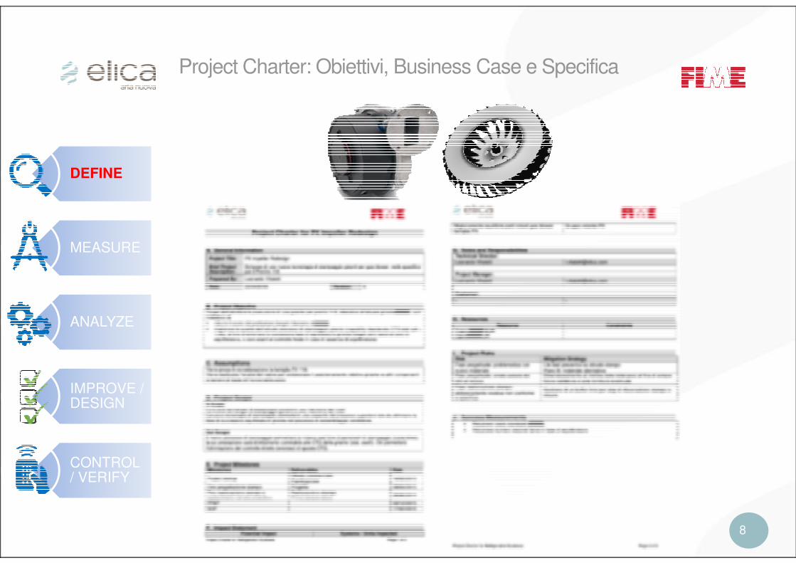
Project Charter: Obiettivi, Business Case e Specifica

10

DEFINE

MEASURE

ANALYZE

IMPROVE / DESIGN

CONTROL / VERIFY

Tecnologia e specifiche tecniche

Squilibrio statico max

Diametro mozzo

Oscillazione

11

DEFINE

MEASURE

ANALYZE

IMPROVE / DESIGN

CONTROL / VERIFY

Casi in esame

12

DEFINE

MEASURE

ANALYZE

IMPROVE / DESIGN

CONTROL / VERIFY

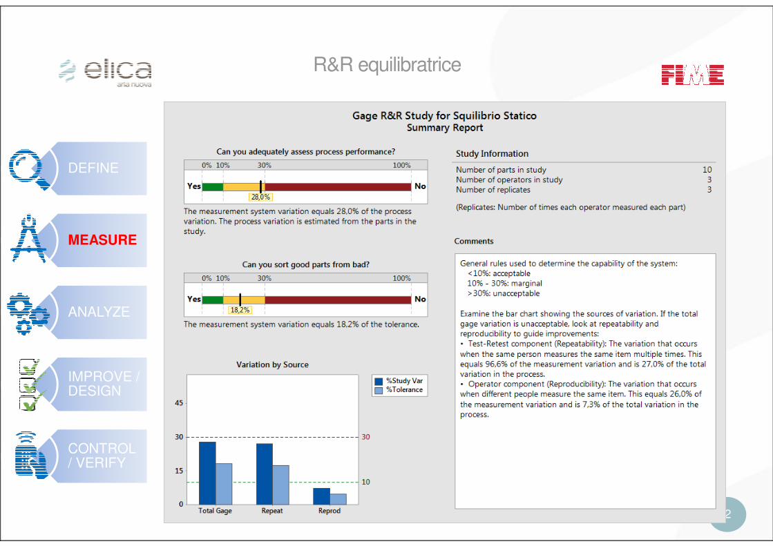
R&R equilibratrice

13

DEFINE

MEASURE

ANALYZE

IMPROVE / DESIGN

CONTROL / VERIFY

Analisi di del processo si stampaggioConfronto tra le tecnologie (1)

S.G. S.G.

H.I. H.I.

1,27

0,83

14

DEFINE

MEASURE

ANALYZE

IMPROVE / DESIGN

CONTROL / VERIFY

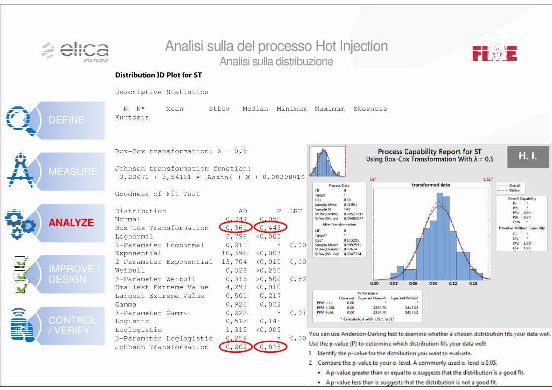
Distribution ID Plot for ST

Descriptive Statistics

N N* Mean StDev Median Minimum Maximum Skewness

Kurtosis

Box-Cox transformation: λ = 0,5

Johnson transformation function:

-3,23071 + 3,54161 × Asinh( ( X + 0,00308819 ) / 0,0123969 )

Goodness of Fit Test

Distribution AD P LRT P

Normal 0,749 0,050

Box-Cox Transformation 0,361 0,443

Lognormal 2,796 <0,005

3-Parameter Lognormal 0,211 * 0,000

Exponential 16,396 <0,003

2-Parameter Exponential 13,704 <0,010 0,000

Weibull 0,328 >0,250

3-Parameter Weibull 0,315 >0,500 0,822

Smallest Extreme Value 4,299 <0,010

Largest Extreme Value 0,501 0,217

Gamma 0,920 0,022

3-Parameter Gamma 0,222 * 0,010

Logistic 0,518 0,148

Loglogistic 1,315 <0,005

3-Parameter Loglogistic 0,259 * 0,000

Johnson Transformation 0,202 0,878

H. I.

Analisi sulla del processo Hot InjectionAnalisi sulla distribuzione

15

DEFINE

MEASURE

ANALYZE

IMPROVE / DESIGN

CONTROL / VERIFY

7654321

N Lotto

Interval Plot of ST vs N Lotto95% CI for the Mean

standard deviations are used to calculate the intervals.

H. I.

H. I.

Analisi sulla del processo Hot InjectionANOVA

16

DEFINE

MEASURE

ANALYZE

IMPROVE / DESIGN

CONTROL / VERIFY

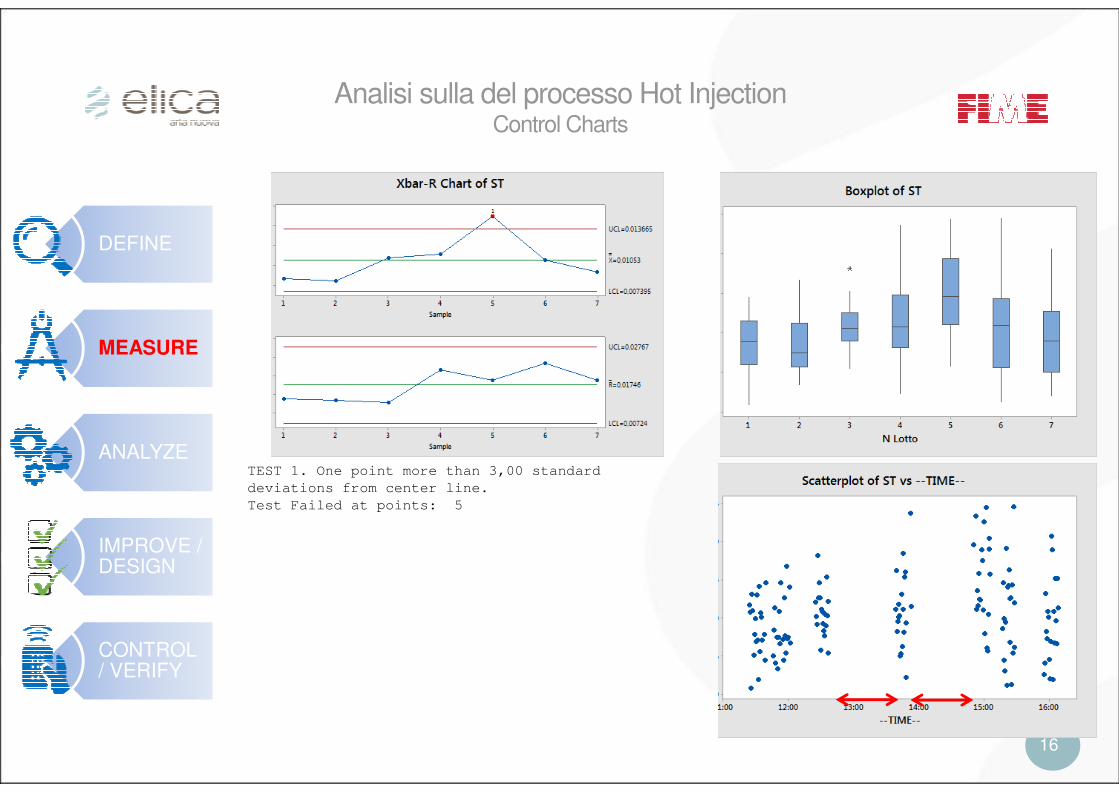
Analisi sulla del processo Hot InjectionControl Charts

TEST 1. One point more than 3,00 standard

deviations from center line.

Test Failed at points: 5

17

DEFINE

MEASURE

ANALYZE

IMPROVE / DESIGN

CONTROL / VERIFY

Analisi sulla del processo Hot InjectionIpotesi sulla variabilità tra lotti

Flu

idit

à(p

rop

orz

ion

ale

a 1

/vis

cosi

tà;

mis

ura

ta in

mm

di s

corr

ime

nto

de

l m

ate

ria

le s

u u

na

spir

ale

)Umidità relativa [%]

Fluidità vs Umidità relativa

18

DEFINE

MEASURE

ANALYZE

IMPROVE / DESIGN

CONTROL / VERIFY

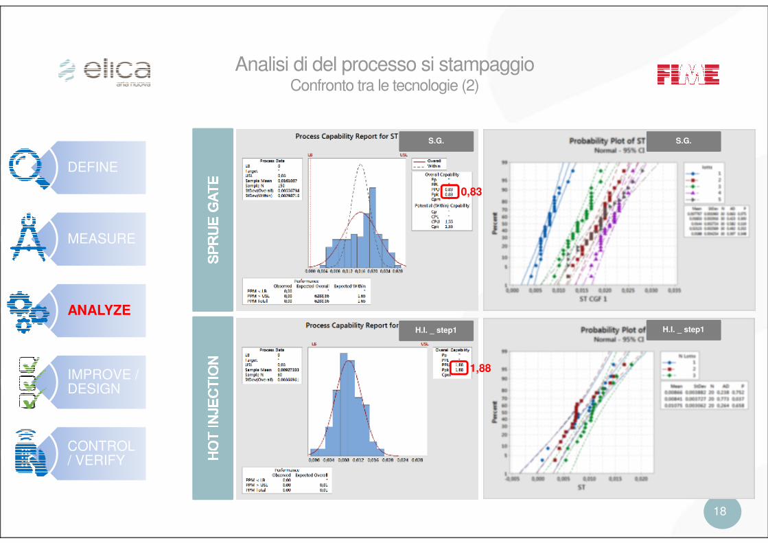
Analisi di del processo si stampaggioConfronto tra le tecnologie (2)

S.G. S.G.

H.I. H.I.

1,27

0,83

1,88

H.I. _ step1 H.I. _ step1

19

DEFINE

MEASURE

ANALYZE

IMPROVE / DESIGN

CONTROL / VERIFY

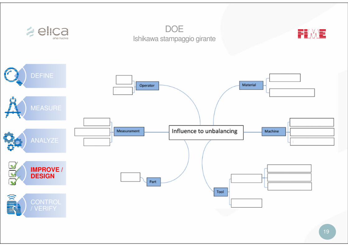
DOEIshikawa stampaggio girante

20

DEFINE

MEASURE

ANALYZE

IMPROVE / DESIGN

CONTROL / VERIFY

DOE Schema funzionale stampaggio girante

T Pc Pm

Parametri di controllo (input e noise)

x1 x2 xn

Parametri intermedi di funzionamento

X1 X2 Xn

Prestazione finale da ottimizzare

Y1 Y2 Yn

t

t_Tmax

Pmax

Squilibrio ST Peso

H. I. P

RO

CE

SS

Oscillazione

Tmax

T_Pmax

T_amb: costante

Materia Prima: singolo batchTempo di essiccamento

v

FULL FACTORIAL PLAN – 5 factors

MEAN & VARIABILITY ANALYSIS – 5 trials per factor

21

DEFINE

MEASURE

ANALYZE

IMPROVE / DESIGN

CONTROL / VERIFY

DOEAnalisi Correlazione parametri intermedi di funzionamento

Correlation: Stat; Oscill.; Weight; Tm; t_Tm; Pm; t_Pm

Stat Oscill. Weight Tmax t_Tmax Pmax

Oscill. 0,128

0,125

Weight -0,769 -0,125

0,000 0,133

Tmax -0,064 -0,289 0,243

0,424 0,000 0,002

t_Tmax -0,349 0,070 0,396 -0,070

0,000 0,400 0,000 0,380

Pmax -0,742 -0,400 0,859 0,299 0,297

0,000 0,000 0,000 0,000 0,000

T_Pmax 0,191 0,093 -0,178 -0,170 0,733 -0,178

0,016 0,264 0,024 0,032 0,000 0,024

Cell Contents: Pearson correlation

P-Value

22

DEFINE

MEASURE

ANALYZE

IMPROVE / DESIGN

CONTROL / VERIFY

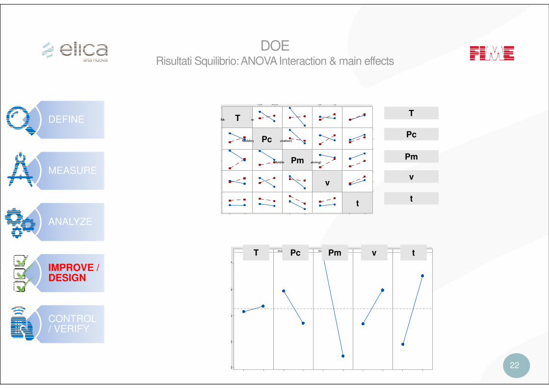
DOERisultati Squilibrio: ANOVA Interaction & main effects

3010

1150950 7030

300270 1050500

Molding Temperature

Molding pressure (commutation)

Molding pressure (maintaining)

Injction speed

Cooling time

7

6

5

4

3

Molding Temperature Molding pressure (commutation) Molding pressure (maintaining) Injction speed Cooling time

T

Pc

Pm

t

v

T Pc Pm tv

T

Pc

Pm

t

v

23

DEFINE

MEASURE

ANALYZE

IMPROVE / DESIGN

CONTROL / VERIFY

DOEFactorial Design Analisi

DOE STAT - 5 TERM

Model Summary

S R-sq R-sq(adj) R-sq(pred)

0,0052046 54,88% 49,24% 40,91%

DOE OSCILL - 5 TERM

Model Summary

S R-sq R-sq(adj) R-sq(pred)

0,0312392 89,54% 87,95% 86,00%

DOE WEIGHT - 5 TERM

Model Summary

S R-sq R-sq(adj) R-sq(pred)

0,166853 97,97% 97,64% 97,26%

Term

ABCD

ABDE

ABCDE

AD

ACDE

BDE

AB

E

ACE

BD

ABC

D

BC

C

AC

76543210

A Molding Temperature

B Molding pressure (commutation)

C Molding pressure (maintaining)

D Injction speed

E Cooling time

Factor Name

Standardized Effect

1,448

Pareto Chart of the Standardized Effects(response is Stat; α = 0,15)

0,010,00-0,01

99,9

99

90

50

10

1

0,1

Residual

Pe

rce

nt

0,0300,0250,0200,0150,010

0,010

0,005

0,000

-0,005

-0,010

Fitted Value

Re

sid

ua

l

0,0080,0040,000-0,004-0,008-0,012

20

15

10

5

0

Residual

Fre

qu

en

cy

160

150

140

130

120

110

1009080706050403020101

0,010

0,005

0,000

-0,005

-0,010

Observation Order

Re

sid

ua

l

Normal Probability Plot Versus Fits

Histogram Versus Order

Residual Plots for Stat

A: T

B: Pc

C: Pm

E: t

D: v

24

DEFINE

MEASURE

ANALYZE

IMPROVE / DESIGN

CONTROL / VERIFY

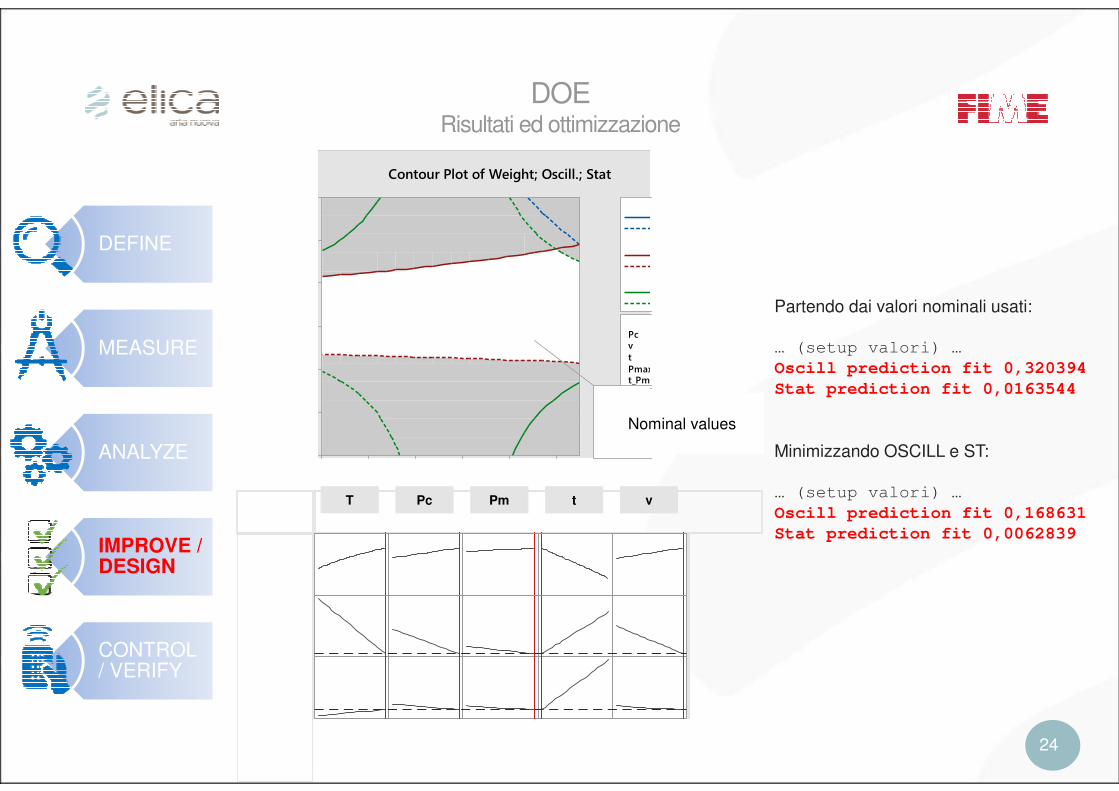
DOERisultati ed ottimizzazione

Partendo dai valori nominali usati:

… (setup valori) …

Oscill prediction fit 0,320394

Stat prediction fit 0,0163544

Minimizzando OSCILL e ST:

… (setup valori) …

Oscill prediction fit 0,168631

Stat prediction fit 0,0062839

Pcv

t

Pmaxt_Pma

1000900800700600500

Contour Plot of Weight; Oscill.; Stat

Molding

Molding

Weight =

Oscill. =

Stat = 0,

Nominal values

PRESS Max = 325,7 time PRESS Max = 3,777

T Pc Pm t v

25

DEFINE

MEASURE

ANALYZE

IMPROVE / DESIGN

CONTROL / VERIFY

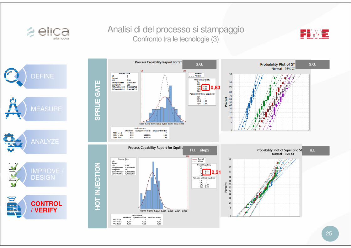
Analisi di del processo si stampaggioConfronto tra le tecnologie (3)

S.G. S.G.

H.I. H.I.

1,27

0,83

1,88

H.I. _ step1

0,0280,0240,0200,0160,0120,0080,004

LSL *Target *USL 0,03Sample Mean 0,00939111Sample N 90StDev(Overall) 0,00310992StDev(Within) 0,00311867

Process Data

Pp *PPL *PPU 2,21Ppk 2,21Cpm *

Cp *CPL *CPU 2,20Cpk 2,20

Potential (Within) Capability

Overall Capability

PPM < LSL * * *PPM > USL 0,00 0,00 0,00PPM Total 0,00 0,00 0,00

Observed Expected Overall Expected WithinPerformance

USL

OverallWithin

Process Capability Report for Squilibrio Statico

0,0200,0150,0100,0050,000

99

95

90

80

70

60

50

40

30

20

10

5

1

Pe

rce

nt

Probability Plot of Squilibrio StNormal - 95% CI

2,21

H.I. _ step2

26

DEFINE

MEASURE

ANALYZE

IMPROVE / DESIGN

CONTROL / VERIFY

Analisi sulla Variabilità

ation) Molding pressure (maintaining) Injction speed Cooling time

1150

950

1150

950

1050

500

1050

500

1050

500

1050

500

70

30

70

30

70

30

30

70

30

70

30

70

30

30

30

3010

3010

3010

30

3010

3010

10

3010

3010

3010

30

3010

3010

0,60,50,40,30,20,10,0

P-Value 0,997

P-Value 0,859

Multiple Comparisons

Levene’s Test

ding Temperature; Molding pressure (commutation); Molding pressure (maiMultiple comparison intervals for the standard deviation, α = 0,05

If intervals do not overlap, the corresponding stdevs are significantly different.

ation) Molding pressure (maintaining) Injction speed Cooling time

1150

950

1150

950

1050

500

1050

500

1050

500

1050

500

70

30

70

30

70

30

70

30

70

30

70

30

70

30

30

30103010

30103010

3010301030103010

30103010

30103010

303010

3010

2,01,51,00,50,0

P-Value 0,000

P-Value 0,344

Multiple Comparisons

Levene’s Test

lding Temperature; Molding pressure (commutation); Molding pressure (maMultiple comparison intervals for the standard deviation, α = 0,05

If intervals do not overlap, the corresponding stdevs are significantly different.

e

0000

0000

00000000

0000

0000

00000

0,040,030,020,010,00

P-Value 0,095

P-Value 0,820

Multiple Comparisons

Levene’s Test

commutation); Molding pressure (mainor the standard deviation, α = 0,05

ignificantly different.

Pc Pm v t

Squilibrio STOscillazione

Peso

27

DEFINE

MEASURE

ANALYZE

IMPROVE / DESIGN

CONTROL / VERIFY

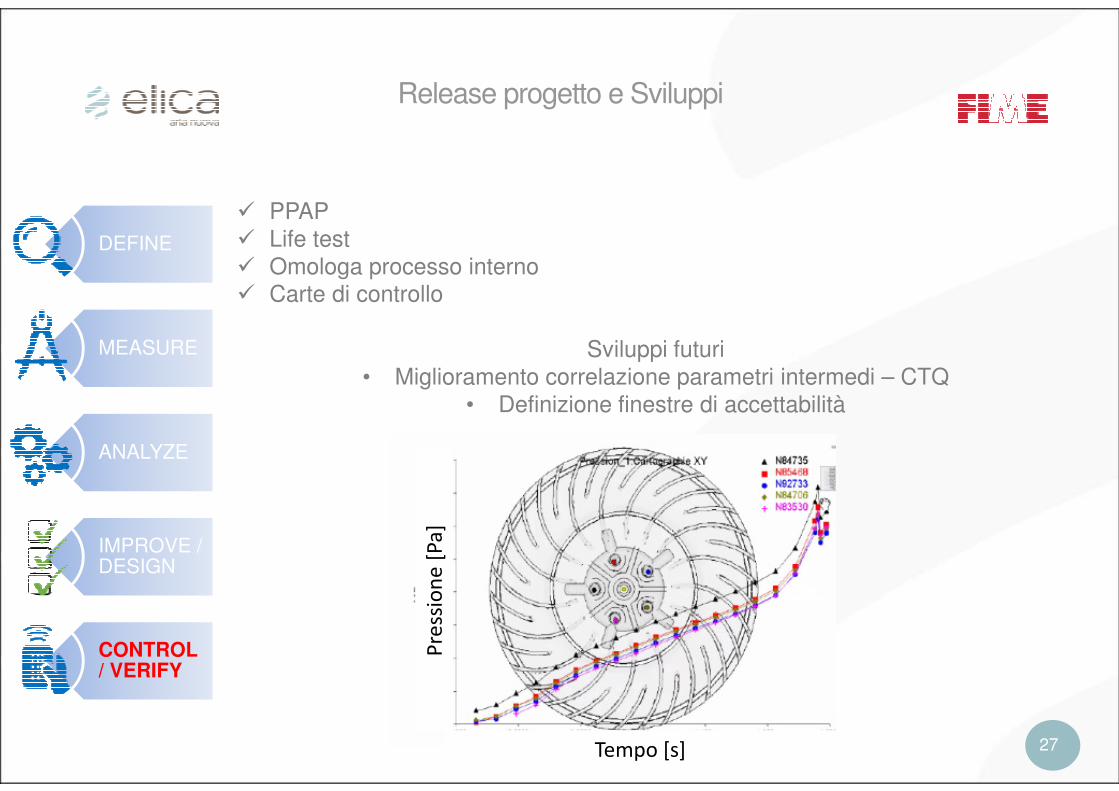
Release progetto e Sviluppi

� PPAP

� Life test

� Omologa processo interno� Carte di controllo

Sviluppi futuri

• Miglioramento correlazione parametri intermedi – CTQ

• Definizione finestre di accettabilità

Pre

ssio

ne

[P

a]

Tempo [s]

28

The future belongsto those who believe in the beauty of their dreams

Eleanor Roosevelt

Thank You

Leonardo Vitaletti – R&D Manager Fans & Motors