Explicit Feature Mapping via Multi-Layer Perceptron and its Application to Mine-Like Objects Detection

Hang Shao and Nathalie Japkowicz

School of Electrical Engineering and Computer Science, University of Ottawa,

Ottawa, Canada hshao068@uottawa.ca, nat@eecs.uottawa.ca

Abstract—In this paper, a novel learning method is introduced that borrows simultaneously from the principles of kernel methods and multi-layer perceptron. Specifically, the method implements the feature mapping idea of kernel methods into a multi-layer perceptron. Unlike in kernel learning where the feature space is usually invisible and inaccessible, the multi-layer perceptron based mapping is explicit. Therefore, the proposed model can be learned directly in feature space. Together with the inherent sparse representation, the proposed approach will thus be much faster and easier to train even in the event of a large network size. The proposed approach is applied in the context of an Autonomous Underwater Vehicle Mine-Like Objects detection task. The results show that the proposed approach is able to improve upon the generalization performance of neural network based methods. Its prediction results are also close to or better than those obtained by kernel machines. Its learning and classification speed is shown to far surpass those of kernel machines. These results are confirmed on a number of experiments involving benchmarking UCI domains.

Keywords— Machine learning; Feature mapping; Neural networks; Kernel learning; Target detection.

I. INTRODUCTION Kernel machines represent a large family of machine

learning methods that has been successfully applied to a wide variety of pattern recognition problems [1]. The non-linear kernel machines usually proceed via two steps. The first step projects the data from the input space to another feature space. The second step learns a model in this new feature space using certain optimization techniques. In this fashion, the nonlinear hyper-surface in the original input space, or decision boundary in classification, can be approximated by a linear hyper-plane in another feature space, usually with a higher dimensionality. In most cases, the feature mapping has to be non-linear in order to perform the non-linear to linear transformation.

Even though the feature space is visible for some kernels, for instance the linear kernel, the kernel machines can process without having access to the feature space. In this way, the curse of dimensionality can be avoided by transferring the feature space computation back to the original input space, making it possible to work with a feature space having a considerable high dimensionality. In kernel machines, the feature mapping is usually implicit. Therefore, kernel machines work without knowing the higher dimensional feature space.

The training process of the kernel machine is to solve for the coefficients associated with the some training points (known as support points in SVMs), based on which the decision boundary is truly built [2]. Since the kernel feature space can be invisible, in the training stage, the higher dimensional computation has to be realized by pair-wise evaluation of the kernel function on the N training data points, where N is the number of training instances. Consequently, an N square sized kernel matrix, also known as Gram matrix is built. The training process can be slow or even virtually impossible if learning is conducted on a large scale dataset where N becomes very large. Unfortunately in many real life applications, it is necessary to deal with the cases where the number of training samples is very large. Therefore, a lot of work has focused on how to speed up kernel learning, especially on the large scale datasets.

When making predictions, the testing data is classified in the same feature space where the decision boundary is learned. As a result of kernel feature mapping, a part of the training data points need to be kept to mathematically express the decision boundary. For non-sparse kernel machines, such as LS-SVMs, the whole dataset has to be stored. Apart from the training points, the same amount of coefficients associated with the support points has to be solved and stored as well. When a new testing point comes, the classification process will compare it with such points via the kernel function and then evaluated with the corresponding coefficients For non-sparse kernel machines, such operation is conducted between the testing point and every training point one by one. Altogether, this makes for a slow classification process.

However, it is important to note that kernel methods are not the only way to perform feature mapping. In certain cases, we might benefit from making the feature mapping explicit where the feature space become visible and accessible. Therefore, directly solving the classifier in such a feature space becomes computationally feasible and, sometimes, even more efficient. Furthermore, since prediction is performed in the same visible space, no training data has to be kept for the testing stage. This work will show how to properly perform explicit feature mapping via building Multi-Layer Perceptron (MLP). Some inherent property of MLP feature mapping is property discussed and addressed in this work. A robust maximum margin classifier is built in the feature space with a high efficiency and competitive generalization performance.

2014 International Joint Conference on Neural Networks (IJCNN) July 6-11, 2014, Beijing, China

978-1-4799-1484-5/14/$31.00 ©2014 IEEE 1055

II. RELATED WORK Due to the slow speed of kernel learning on large scale datasets, previous research resorted to better or more efficient optimization techniques, such as decomposition methods, to solve kernel machines [3-5]. Another approach is to use data dependent low-rank approximation to reduce the size of kernel matrix [6, 7]. This way, the feature mapping can be regarded as explicit. When making the feature mapping explicit, no decomposition techniques are needed. The projection coefficients can be directly copied from the subset of the original training data. The subset selection can be either conducted by certain optimization criteria [8] or simply by sampling [9].

Vedaldi et al. [10] have also discussed the limitation of non-linear kernel mapping on large scale datasets. Explicit feature mapping is used in order to approximate a family of addictive kernels, such as the intersection kernels and χ2 kernels. A closed-form expression of the mapping function is derived for such kernels. The analysis of the approximation error is also presented.

Some random mapping methods can be viewed as another kind of explicit feature mapping. In such methods, the feature projection is random. Rahimi et al. [11] proposed to use Fourier and Binning features to transform the data to a low dimensional random feature space. A regression model is built after the random feature mapping is completed.

Two neural network based methods, Extreme Learning Machine (ELM) [12] and Echo State Networks (ESN) [13] are also examples of random feature mapping learning. The mapping in such random methods will be independent of the data. Both methods contain a random reservoir which consists of many hidden neurons, and the only trainable part is the weights in the linear output layer. ELM is often used in static problems. However, as a recurrent neural network, ESN is often applied to solve dynamic problems. The neurons inside the ESN reservoir are sparsely connected. If the sparsity of the internal connection is reduced to 0 and all the feedback weights are removed, ESN will share the same network architecture as ELM. It is worth mentioning that ELM is proven to be a universal approximator with random hidden layer.

It worth mentioning that the combination of MLP and margin maximization is not new. There are also similar works using MLP and max margin classifier (like SVMs) in joint. An example of such work can be found in digit recognition [14]. MLP is first used to classify the digits, then SVMs is trained on the classification outputs produced by the MLP. In this approach, both the MLP and SVM are used as classifiers and SVM is used to distinguish the results of the MLP, which is much different from the proposed approach. In another MLP-SVM classifier [15], the model training is also divided into two stage. Firstly, the MLP is trained to minimized the relative entropy between the output distribution and the true label distribution. Secondly, SVMs is trained on the outputs of MLP. The first stage MLP training is independent of the SVM. Moreover, either from the objective function or the optimization method, the proposed approach is different from such works. More importantly, the norm of MLP weights will be addressed in the proposed approach.

III. THE PROPOSED APPROACH As mentioned above, some neural network based methods

can be viewed as a good case of explicit feature mapping. Therefore, we can perform the mapping via building such networks. In this work, we will show how to implement explicit mapping via building one of the most widely applied neural networks, the MLP. The feature space will be defined by the parameters and activation function of the MLP hidden layer(s).

However, the proposed approach does not belong to the family of random mapping networks such as ELM or ESN. The proposed approach will not use random and data-independent feature mapping. A relationship between the training points and the mapping parameters will be built, as we will later see the impact of such parameters on the final learning model.

Furthermore, it is worth mentioning that unlike some of the related works, from the starting point, we are not using explicit feature mapping to approximate any kernels, nor is it any kind of speed-up version of kernel learning, since no kernel will be used in the proposed approach at all. The proposed method in this work is neural network based and it will show how to properly implement the explicit feature mapping via building MLP. We are not approximating any kernels, so the MLP-based explicit feature mapping enjoys more flexibility. MLP is picked in this work because the architecture of MLP is well-known and straightforward, making the proposed model easy to understand. However, the explicit feature mapping idea is not limited to MLP cases.

In this research, we will focus on binary classification problems, but it can be easily extended to multi-class or one class classifications. It is worth pointing out that the explicit feature mapping is also ready and easy to be applied to most of the learning tasks where kernel learning is valid, such as regression analysis and Principal Component Analysis (PCA), etc.

While implementing the explicit feature mapping via building MLP, we cannot ignore certain properties of MLP. The generalization ability of MLP is closely related to the norm of the weights. The main parameters in MLP are its weights. Thus, it will be beneficial to take into account the impact of the weights on the final network. Moreover, the dimensionality of the feature space is expected to be large. As a result, another property of the MLP used in this work is that it has a large hidden layer, which differs from the traditional MLP. The proposed method will seek to produce a maximum margin classifier, which maximizes the separation space between the positive class and the negative class. Furthermore, a sparse and robust solution will be obtained. The decision boundary will only be built on a part of the training points, which will speed up the training process. The sigmoid neurons, the most common neuron in the MLP will be used in the hidden layer. We will begin by building MLP with single hidden layer, and the proposed approach will be extended to deep networks with ease where multiple hidden layers are included in the architecture.

1056

A. Explicit feature mapping via Multi-Layer Perceptron For simplicity, we can begin with the case of MLP with

single hidden layer. Given N training instances (xi, ti), xi∈RM, ti∈{-1, 1}, (i=1,2,…, N), where xi are the attributes, M is the number of attributes and ti is the class label, using a linear output layer, the output yj of a MLP with L hidden nodes is

1

( , ), 1, 2, ..., (1)L

j i i ji

y w g j N=

= =∑ a x

The input weights connected to the ith hidden neuron are ai (the hidden bias can be included in the input weights), wi is the output weights and g(a, x) is the hidden layer activation function, which is set to be the sigmoid function in this study. The definition of sigmoid is

T

1( , ) (2)

1 exp( )g =

+ −a x

a x

Similarly to SVMs, the objective function is defined to penalize the wrongly classified points and those lying inside the separating margin. Weight decay is applied as a form of regularization.

2 2

1 21 1 1 1

1min ( , ) [ ( ) ] .

2

( ) 1 , 1, 2, ..., (3)

N L L M

i i iji i i j

i i i

L E w a const

subject to t y i N

ξ λ λ

ξ= = = =

= + + +

= − =

∑ ∑ ∑∑w a

x

where λ1 and λ2 are the regularization parameters, M is the number of input neurons w=[w1,w2,…,wL]T. As we can see, the proposed approach has included both the training error and the norm of weights in the objective function. Minimizing the weights w is equivalent to maximizing the separating margin between the positive and negative class in the hidden layer feature space, and the proposed approach will result in a maximum margin classifier.

The input weights aij will directly impact on the nonlinearity of the hidden layer feature mapping, which will be discussed later. Considering the large noise of the data in our application domain, the error function is chosen to be a robust one-side Huber function [16] defined as

20.5 ,

2( ) 0.5 , 0

0 , 0

(4)

u u u

E u

ξ ξ

ξ ξ ξ

ξ

− >

= ≤ ≤

<

⎧⎪⎪⎨⎪⎪⎩

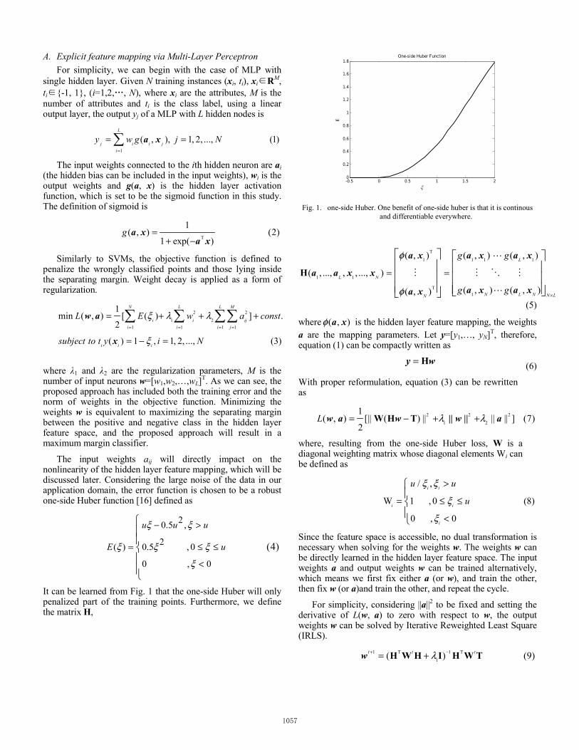
It can be learned from Fig. 1 that the one-side Huber will only penalized part of the training points. Furthermore, we define the matrix H,

-0.5 0 0.5 1 1.5 20

0.2

0.4

0.6

0.8

1

1.2

1.4

1.6

1.8

ξ

E

One-side Huber Function

Fig. 1. one-side Huber. One benefit of one-side huber is that it is continous and differentiable everywhere.

T

1 1 1 1

1 1

T1

( , ) ( , ) ( , )

( , ..., , , ..., )

( , ) ( , )( , )

L

L N

N L N N LN

g g

g g×

= =

⎡ ⎤ ⎡ ⎤⎢ ⎥ ⎢ ⎥⎢ ⎥ ⎢ ⎥⎢ ⎥ ⎢ ⎥⎣ ⎦⎣ ⎦

H

a x a x a x

a a x x

a x a xa x

φ

φ (5)

where ( , )a xφ is the hidden layer feature mapping, the weights a are the mapping parameters. Let y=[y1,…, yN]T, therefore, equation (1) can be compactly written as

= Hy w (6)

With proper reformulation, equation (3) can be rewritten as

2 2 2

1 2

1( , ) [|| ( ) || || || ] (7)

2L λ λ= − + +W H Tw a w || w || a

where, resulting from the one-side Huber loss, W is a diagonal weighting matrix whose diagonal elements Wi can be defined as

/ ,

W 1 , 0 (8)

0 , 0

i i

i i

i

u u

u

ξ ξ

ξ

ξ

>

= ≤ ≤

<

⎧⎪⎨⎪⎩

Since the feature space is accessible, no dual transformation is necessary when solving for the weights w. The weights w can be directly learned in the hidden layer feature space. The input weights a and output weights w can be trained alternatively, which means we first fix either a (or w), and train the other, then fix w (or a)and train the other, and repeat the cycle.

For simplicity, considering ||a||2 to be fixed and setting the derivative of L(w, a) to zero with respect to w, the output weights w can be solved by Iterative Reweighted Least Square (IRLS).

1 T 1 T

1( ) (9)t t tλ+ −= +H W H I H W Tw

1057

As previously stated, we do not want to use random feature mapping, so the mapping parameters aij need to be trained. There are many valid methods to train such parameters. In this work, we pick one of the most well-known methods, error backpropagation (BP) [17]. The only difference is that since the error function is not quadratic anymore and aij is included in the objective function, the delta term of the output layer has to be weighted according to (8) before backpropagated. Also the aij have to be decayed according to their regularization parameter λ2. The rest deriving process and learning formulas will remain the same to traditional error backpropagation.

B. Insight into the impact of the norm of weights The property of the MLP-based explicit feature mapping is

directly related to the norm of MLP weights. It has been pointed out that when reaching small training errors, MLP with a smaller norm of weights is more likely to generalize well [18]. In this case, if the norm of input weights is large, the sigmoid function in the hidden layer will be saturated, and it will produce an output either too close to 0 or 1. Any variation in the input data will be magnified by the weights and cause the output hidden neurons to alternate between 0 and 1, leading to a great variation in the output. Such network is very likely to memorize and overfit, as any source of noise and error will be heavily magnified.

In this work, a large MLP is built to implement the explicit feature mapping. As a result of the learning ability of such large network, it is easy to reach small training error after a very few cycles of weights training. At this point, keep tuning the input weights to minimize the training error is not necessary because of the danger of overfitting. We keep the input weights small at the moment and directly compute w via (9), so the learning speed of the proposed approach can be very fast.

From another perspective, the impact of a is more obvious in regression problems. Given a testing point x*, with the same feature mapping defined by (5), the predicted output can be written as

* T *( , )y = w a xφ (10) Solving w with ridge regression, equation (10) can be rewritten as

* * T T 1 *

11 1

( , ) ( ) ( , ) ( , ) (11)N N

i i i ii i

y t k tλ −

= =

+ =∑ ∑H H I= a x a x x xφ φ

where * T T 1

1( , ) ( ) ( , )i itλ −+H H Ia x a xφ φ is known as the equivalent kernel [19]. It is interesting to find from (11) that the predictive output y* is in fact a linear combination of ti, the labels of the training instances. The shape of k(x*, xi) will be largely affected by the norm of the input weights a, which will further support the previous discussion and cast light on why networks with large weights are more likely to overfit. The behaviour of the network is very similar to k-Nearest Neighbour (k-NN).

-5 -4 -3 -2 -1 0 1 2 3 4 50

0.1

0.2

0.3

0.4

0.5

0.6

0.7

0.8

0.9

1Sigmoid

Fig. 2. The working region of the sigmoid is shown by the red dashed lines. The sigmoid will be close to a linear function that could be approximated by the blue line if its input is close to 0. More non-linearity and complexity is gained if the sigmoid works in a wider region.

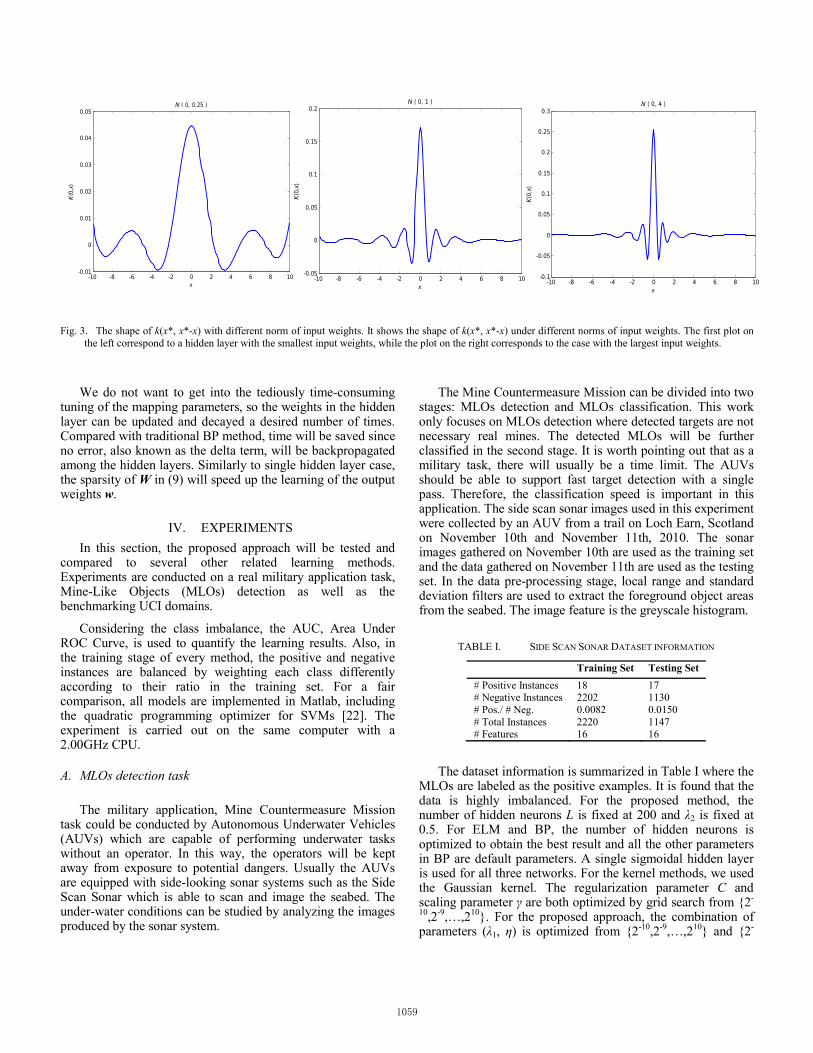
As shown in the left plot in Fig. 3, when the norm of the input weights is small, the smooth k(x*, x*-x) will result in a flexible network that could take into account more distant data points. The predicted output is a weighted average of a lot of nearby training points, which is similar to a large k in k-NN. When the norm of the input weights increases, the k(x*, x*-x) becomes more peaked and localized, as illustrated by the right plot. In such cases, the predicted output will largely weigh only a few data points that are closest to the testing sample x*, which is more likely to lead to overfitting. The network will converge to 1-Nearest-Neighbour if ||a|| is sufficiently large. The role of a here is similar to that of the smoothing parameter used in Parzen’s probability density function estimation, which serve as a trade-off between the bias and variance of the estimator.

It is worth mentioning that the above discussion as well as such a property is only limited to sigmoidal hidden layers. When using other hidden neurons, this property may not hold anymore.

C. Extension to deep architecture

As mentioned before, we can also easily extend the proposed approach to a deep architecture with multiple layers. In deep learning methods [20, 21], the Restricted Boltzmann Machine or auto-encoders can be trained at each layer on unlabelled dataset, and the final layer is tuned in a supervised way, such as logistic regression or softmax regression, on labeled dataset.

Similarly, we can also stack additional feedforward layers one at a time onto the previously trained architecture to form a deep network. However, currently we work on labeled datasets, the hidden layer of the proposed approach is trained in a supervised way. Similarly to other deep learning methods, the output of the previously trained layer is regarded as new input data for the next additional layer, so the learning consists, in fact, of repeating the training procedure of the single hidden layer case as described in section A. At this point, the proposed approach is the same as that of the other deep learning methods.

1058

-10 -8 -6 -4 -2 0 2 4 6 8 10-0.01

0

0.01

0.02

0.03

0.04

0.05

x

K(0

,x)

N ( 0, 0.25 )

-10 -8 -6 -4 -2 0 2 4 6 8 10-0.05

0

0.05

0.1

0.15

0.2

x

K(0

,x)

N ( 0, 1 )

-10 -8 -6 -4 -2 0 2 4 6 8 10-0.1

-0.05

0

0.05

0.1

0.15

0.2

0.25

0.3

x

K(0

,x)

N ( 0, 4 )

Fig. 3. The shape of k(x*, x*-x) with different norm of input weights. It shows the shape of k(x*, x*-x) under different norms of input weights. The first plot on the left correspond to a hidden layer with the smallest input weights, while the plot on the right corresponds to the case with the largest input weights.

We do not want to get into the tediously time-consuming tuning of the mapping parameters, so the weights in the hidden layer can be updated and decayed a desired number of times. Compared with traditional BP method, time will be saved since no error, also known as the delta term, will be backpropagated among the hidden layers. Similarly to single hidden layer case, the sparsity of W in (9) will speed up the learning of the output weights w.

IV. EXPERIMENTS In this section, the proposed approach will be tested and

compared to several other related learning methods. Experiments are conducted on a real military application task, Mine-Like Objects (MLOs) detection as well as the benchmarking UCI domains.

Considering the class imbalance, the AUC, Area Under ROC Curve, is used to quantify the learning results. Also, in the training stage of every method, the positive and negative instances are balanced by weighting each class differently according to their ratio in the training set. For a fair comparison, all models are implemented in Matlab, including the quadratic programming optimizer for SVMs [22]. The experiment is carried out on the same computer with a 2.00GHz CPU.

A. MLOs detection task

The military application, Mine Countermeasure Mission task could be conducted by Autonomous Underwater Vehicles (AUVs) which are capable of performing underwater tasks without an operator. In this way, the operators will be kept away from exposure to potential dangers. Usually the AUVs are equipped with side-looking sonar systems such as the Side Scan Sonar which is able to scan and image the seabed. The under-water conditions can be studied by analyzing the images produced by the sonar system.

The Mine Countermeasure Mission can be divided into two stages: MLOs detection and MLOs classification. This work only focuses on MLOs detection where detected targets are not necessary real mines. The detected MLOs will be further classified in the second stage. It is worth pointing out that as a military task, there will usually be a time limit. The AUVs should be able to support fast target detection with a single pass. Therefore, the classification speed is important in this application. The side scan sonar images used in this experiment were collected by an AUV from a trail on Loch Earn, Scotland on November 10th and November 11th, 2010. The sonar images gathered on November 10th are used as the training set and the data gathered on November 11th are used as the testing set. In the data pre-processing stage, local range and standard deviation filters are used to extract the foreground object areas from the seabed. The image feature is the greyscale histogram.

TABLE I. SIDE SCAN SONAR DATASET INFORMATION

Training Set Testing Set # Positive Instances 18 17 # Negative Instances 2202 1130 # Pos./ # Neg. 0.0082 0.0150 # Total Instances 2220 1147 # Features 16 16

The dataset information is summarized in Table I where the MLOs are labeled as the positive examples. It is found that the data is highly imbalanced. For the proposed method, the number of hidden neurons L is fixed at 200 and λ2 is fixed at 0.5. For ELM and BP, the number of hidden neurons is optimized to obtain the best result and all the other parameters in BP are default parameters. A single sigmoidal hidden layer is used for all three networks. For the kernel methods, we used the Gaussian kernel. The regularization parameter C and scaling parameter γ are both optimized by grid search from {2-

10,2-9,…,210}. For the proposed approach, the combination of parameters (λ1, η) is optimized from {2-10,2-9,…,210} and {2-

1059

10,2-9,…,20}, where η is the learning rate used to update the mapping parameters aij.

Table II shows the comparison of the results on the testing data. The True Positive Rate (TPR) and False Positive Rate (FPR) are also given for reference. Table III shows the model parameters as well as the training and classification times (LR in the tables is short for Logistic Regression). From the result tables we can see that LR it has the lowest AUC. It is the only classifier that directly solves the problem in the original input space. The proposed approach is able to beat all other neural network based models in prediction performance. The proposed approach can produce a prediction result close to or even better than the results obtained by kernel methods. It is found that the LS-SVMs has the highest AUC, but unfortunately as a non-sparse kernel machine, all the training points will become support vectors, which will limit its detection speed when trained with large scale dataset as previously discussed.

TABLE II. COMPARISON OF PERFORMANCE ON SIDE SCAN SONAR DATA

Method Function TPR FPR AUC SVMs Gaussian 0.8824 0.0442 0.9865 LS-SVMs Gaussian 0.9412 0.0540 0.9885 Kernel LR Gaussian 0.9412 0.0416 0.9858 BP Sigmoid 0.9353 0.3145 0.9231 ELM Sigmoid 0.9059 0.0686 0.9747 LR \ 0.4117 0.1876 0.7989 Proposed Approach Sigmoid 0.9177 0.0443 0.9871

TABLE III. MODEL PARAMETERS AND COMPARISON OF TIME ON SIDE SCAN SONAR DATA

Method pameters sparsity (%)

training time(s)

classification time(s)

SVMs C=2-5,γ=24 27.8 94.17 0.9063 LS-SVMs C=22, γ=22 100 13.07 2.1719 Kernel LR C=2-6,γ=20 100 33.37 2.2031 BP L=20 \ 9.173 0.0313 ELM L=40 \ 0.090 <0.01 LR C=2-2 \ 2.093 <0.01 Proposed Approach

λ1=2-8, η=2-7

48.6 1.123 0.0391

In terms of training and classification times, the proposed method largely outperformed all kernel methods. Moreover, for the proposed approach, the classification speed is directly related to the number of hidden neurons L in the network, which is independent of the size of training set. Therefore, the proposed approach enjoys more flexibility. Its classification speed can be manually adjusted by properly setting the value of L.

B. UCI domains

The proposed approach is a general method, so it can also be applied to many other domains. In this section, the performance of the proposed approach is tested on UCI domains [23]. As no real time classification is required on the UCI domains, we do not record the classification time in this section. The details of the UCI datasets are listed in Table IV. As mentioned before, only binary classification is considered

in this work. Some of the listed datasets were originally used for multiple classifications, so for such datasets multiple classes are merged into two classes.

Before training, all attributes are normalized into the interval [-1, 1]. The proposed approach is compared to two classic neural network and kernel methods, BP and SVMs. The result of another neural network based on random feature mapping methods, ELM is also given. A grid search is conducted to optimize the parameters of SVMs (C and γ, both within{2-10,2-9,…,210}) and the proposed approach (λ1 and η). For single hidden layer case, λ1 and η are optimized within {2-

10,2-9,…,210} and {2-10,2-9,…,20}. For multi-layer case, they are optimized within {2-10,2-9,…,210} and {2-20,2-15,…,20}. The number of hidden nodes L used for the proposed approach is set to a large number, without much careful optimization. Other experiment settings remain the same to the previous section for the side scan sonar data.

TABLE IV. UCI DATASETS INFORMATION

Dataset

Attributes # pos. Instance

# neg. Instance

# pos./ # neg. real integer

WDBC 0 9 239 444 0.5283 CMC 0 9 629 844 0.7453 CTG 0 20 1655 471 3.514 Diabetes 2 6 268 500 0.538 Glass 9 0 68 146 0.4658 Haber 0 3 225 81 2.778 Image 6 3 1320 990 1.333 Iono 2 2 225 126 1.786 Irish 0 5 175 325 0.5385 Liver 1 5 145 200 0.725 Sat 0 36 918 1082 0.8484 Spam 55 2 1813 2788 0.6503 Wine 11 2 107 71 1.507

TABLE V. COMPARISON OF TRAINING TIME(S) ON UCI DOMAINS

Dataset BP ELM SVMs Proposed Approach Single Multiple

WDBC (Dev.)

1.077 (0.2027)

0.0031 (0.0066)

3.895 (0.6330)

0.2437 (0.0322)

0.2978 (0.0241)

CMC (Dev.)

1.411 (0.3213)

0.1078 (0.0172)

61.24 (2.361)

1.3843 (0.0670)

4.010 (0.1973)

CTG (Dev.)

23.01 (6.127)

0.7437 (0.0692)

85.30 (5.427)

4.0125 (0.5266)

5.572 (0.4654)

Diabetes (Dev.)

0.9078 (0.1830)

0.0047 (0.0075)

8.0922 (1.3124)

0.8409 (0.0656)

2.216 (0.1624)

Glass (Dev.)

0.7813 (0.0979)

0.0019 (0.0060)

0.9687 (0.1462)

0.1562 (0.0165)

0.1828 (0.0232)

Haber (Dev.)

0.675 (0.1296)

0.0016 (0.0007)

2.300 (0.3075)

0.0688 (0.0489)

0.0703 (0.0168)

Image (Dev.)

14.948 (3.558)

0.900 (0.0391)

32.20 (3.096)

1.9860 (0.2907)

2.8381 (0.1959)

Iono. (Dev.)

2.255 (1.190)

0.0172 (0.0049)

3.155 (0.4969)

0.1640 (0.0184)

0.2322 (0.0204)

Irish (Dev.)

0.9989 (0.5665)

0.0031 (0.0066)

9.414 (0.8928)

0.2750 (0.0296)

0.3038 (0.0308)

Liver (Dev.)

0.9934 (0.1409)

0.0051 (0.0080)

2.6406 (0.3212)

0.0913 (0.0179)

0.2456 (0.0251)

Sat (Dev.)

56.68 (4.765)

0.5549 (0.0482)

32.91 (3.247)

0.8037 (0.0515)

3.621 (0.1896)

Spam (Dev.)

111.5 (48.82)

1.973 (0.0347)

461.2 (6.073)

11.05 (1.711)

11.58 (1.179)

Wine (Dev.)

1.313 (0.5420)

0.0034 (0.0065)

0.8953 (0.1409)

0.0336 (0.0186)

0.0625 (0.0071)

1060

TABLE VI. COMPARISON OF MODEL PARAMETERS ON UCI DOMAINS

Dataset BP ELM

SVMs Proposed Approach single multiple

L L C, γ, SVs L, λ1 ,η L1,L2,L3, λ1 ,η WDBC 15 15 2-2,2-8,289 200,24,2-8 20, 200,\,2-1,2-5 CMC 5 60 26,2-4,912 300,20,2-7 40, 500,\,2-2,2-10 CTG 30 150 29,2-2,625 400,2-8,2-9 150, 500,\,2-10,2-20 Diabetes 5 15 23,2-5,415 300,20,2-4 20,100,500,2-1,2-15 Glass 15 10 2-1,24,159 100,24,2-3 10,50,200,2-8,2-10 Haber 5 15 26,2-1,187 100,2-4,2-6 10,100,\,2-10,2-10 Image 20 160 26, 20,257 300,2-10,2-10 150,200,300,2-12,2-20 Iono 10 60 26, 21,248 200,21,2-5 60,100,200,2-2,2-10 Irish 10 15 2-1,26,412 200,2-7,2-1 15,50,200,2-8,2-10 Liver 30 20 210,2-4,204 100,2-6,2-9 20,200,\,2-10,2-10 Sat 35 120 23,2-4,307 200,2-2,2-5 100,500,\,2-1,2-10 Spam 15 150 26,2-1,766 500,2-10,2-10 200,500,\.2-5,2-20 Wine 30 20 2-10,2-4,160 100,2-2,2-10 50,150,\,2-3,2-10

TABLE VII. COMPARISON OF PERFORMANCE (AUC) ON UCI DOMAINS

Dataset BP

ELM

SVMs Proposed Approach single multiple

WDBC (Dev.)

0.9880 (0.0129)

0.9937 (0.0049)

0.9953 (0.0048)

0.9956 (0.0047)

0.9956 (0.0053)

CMC (Dev.)

0.7331 (0.0379)

0.7177 (0.0403)

0.7474 (0.0365)

0.7394 (0.0423)

0.7409 (0.0377)

CTG (Dev.)

0.9109 (0.0295)

0.8898 (0.0241)

0.9351 (0.0192)

0.9295 (0.0185)

0.9407 (0.0213)

Diabetes (Dev.)

0.8106 (0.0650)

0.8308 (0.0427)

0.8359 (0.0406)

0.8367 (0.0496)

0.8366 (0.0562)

Glass (Dev.)

0.8062 (0.1275)

0.8321 (0.1097)

0.8907 (0.0821)

0.8426 (0.1098)

0.8567 (0.1033)

Haber (Dev.)

0.6352 (0.1223)

0.6986 (0.1097)

0.7020 (0.0984)

0.7171 (0.1117)

0.7072 (0.1146)

Image (Dev.)

0.9941 (0.0038)

0.9903 (0.0070)

0.9944 (0.0042)

0.9955 (0.0046)

0.9942 (0.0042)

Iono (Dev.)

0.9307 (0.0514)

0.9381 (0.0418)

0.9799 (0.0221)

0.9670 (0.0329)

0.9683 (0.0382)

Irish (Dev.)

0.9256 (0.0401)

0.9206 (0.0265)

0.9620 (0.0171)

0.9246 (0.0444)

0.9261 (0.0319)

Liver (Dev.)

0.7316 (0.0926)

0.7480 (0.0713)

0.7667 (0.0899)

0.7751 (0.0731)

0.7621 (0.0779)

Sat (Dev.)

0.9838 (0.0122)

0.9803 (0.0090)

0.9864 (0.0069)

0.9842 (0.0070)

0.9885 (0.0061)

Spam (Dev.)

0.9682 (0.0089)

0.9566 (0.0093)

0.9762 (0.0065)

0.9702 (0.0086)

0.9738 (0.0071)

Wine (Dev.)

0.9833 (0.0526)

0.9954 (0.0089)

0.9969 (0.0045)

0.9977 (0.0036)

0.9974 (0.0061)

The results shown are from an experiment of 5×10-fold

cross-validation. Both the average results and the standard deviation (shown in italics in brackets) are recorded. The parameters of each model are given in Table VI. For the proposed approach, both cases with single hidden layer (penultimate column in Table V, Table VI, and Table VII) and multiple hidden layers (last column in Table V, Table VI, and Table VII) are listed. In Table VI, parameters L1, L2, L3 (roughly optimized) indicate the number of neurons in the first, second, third hidden layer counted from the input side. In order to evaluate the results listed in Table VII, statistical tests are performed. To compare multiple algorithms on multiple domains, we chose Friedman’s test and post-hoc (Nemenyi’s) test [24].

First, the Friedman’s test returns a χF2 value of 37.46 and p-

value of 1.45×10-7<0.01. Therefore, the H0 hypothesis that all

the classifiers have similar performance to each other on the datasets is rejected at significance level 0.01.

Furthermore, Nemenyi’s test is conducted. The critical value of qα is 2.83 for α=0.05 and df=48. The result shows that the q statistics between the proposed approach with single hidden layer, and BP and ELM, are both 3.7210 and it is 0.3721 when compared to SVMs. With multiple hidden layers, the q statistics between the proposed approach and BP and ELM are both 3.9691 and it is 0.1240 with SVMs. Therefore, from the result of Friedman’s test and Nemenyi’s test, we can conclude that on the UCI benchmarking datasets, at the significant level of 0.05, the proposed approach, with either single hidden layer or multiple hidden layers outperformed both BP and ELM and tied with SVMs.

We also see that the proposed approach is easy to train. In terms of training times, from the results listed in Table V, we can see that ELM is able to dominate on all datasets. This is because ELM uses random feature mapping and the whole learning process is only a one step calculation of the output layer. The proposed approach will be much faster than that of kernel based methods. Furthermore, even using a much larger network, the proposed approach is able to learn faster than BP on all the datasets with one hidden layer. With multiple layers, it is still faster than BP on most of the datasets.

V. CONCLUSION AND FUTURE WORK

This work proposed a learning model that implements explicit feature mapping via building MLP. It is able to improve the prediction performance of neural network based methods. From our previous discussion in section 3.2, we found that the norm of the mapping parameters, which affects the working region of the sigmoid function, will control the non-linearity of the feature mapping, so it cannot be a random number independent of the training data. It is reasonable and beneficial to look at such parameters when building the network. The proposed approach is able to produce a satisfying generalization result as long as such parameters are properly addressed. Benefiting from no tedious hidden layer training, the learning speed of the proposed approach is very fast.

Moreover, compared to kernel machines, the proposed approach will produce a generalization performance close to that of kernel machines, with much improvement in the learning speed even using a very large network. On the Side Scan Sonar dataset, where it is of great practical importance, the classification speed will also be largely improved. The improvement in training and classification speed is the result of explicit feature mapping which enables the direct feature space computation.

Currently the network architecture of MLP is manually decided. One possible future research avenue could be how to learn the architecture, such as the number of layers and neurons in each layer, directly from the input pattern. Moreover, it is possible to implement the explicit feature mapping via constructing other non-sigmoidal layer(s) or other non-feedforward network architectures. It would be interesting to see how the network parameters would affect the final model. It would also be worth discussing how to properly learn the

1061

mapping parameters in such cases. Another possible future direction could be to apply the explicit MLP feature mapping to other tasks such as one class learning and PCA, etc..

ACKNOWLEDGMENT We would like to thank Dr. Alex Bourque and Dr. Bao

Nguyen, research scientists at Defence Research and Development Canada, who work with us on a research project and provide us the MLOs data.

REFERENCE [1] J. Shawe-Taylor and N. Cristianini, Kernel Methods for Pattern Analysis.

Cambridge University Press, 2004. [2] C. Cortes and V. Vapnik, “Support-vector networks,” Machine learning,

Vol. 20, 1995, pp. 273-297. [3] E. Osuna, R. Freund and F. Girosi, “Training support vector machines:

an application to face detection”, Computer Vision and Pattern Recognition, Proceedings, IEEE Computer Society Conference on, 1997, pp. 130-136.

[4] T Joachims, “Making large scale support vector machine learning practical,” Advances in kernel methods, MIT press, 1999, pp.169-184.

[5] J.C. Platt, “Fast training of support vector machines using sequential minimal optimization,” Advances in kernel methods, MIT press, 1999, pp.185-208.

[6] Y-J Lee and O. L. Mangasarian, “RSVM: Reduced support vector machines,” SIAM International Conference on Data Mining, 2001.

[7] S. Fine and K. Scheinberg, “Efficient SVM training using low-rank kernel representations,” Journal of Machine Learning Research, Vol. 2, 2001, pp.243-264.

[8] A.J. Smola and B. Scholkopf, “Sparse greedy matrix approximation for machine learning,“ Proceedings of the 17th International Conference on Machine Learning. (ICML) , 2000.

[9] D. Achlioptas, F. McSherry and B. Scholkopf, “Sampling Techniques for Kernel Methods,” In: Advances in Neural Information Processing Systems. MIT Press, 2002.

[10] A. Vedaldi and A. Zisserman, “Efficient Additive Kernels via Explicit Feature Maps,” IEEE Trans. Pattern Anal. Mach. Intell. 34(3), 2012, pp. 480-492.

[11] A. Rahimi and B. Recht, “Random Features for Large-Scale Kernel Machines,“ In: Neural Information Processing Systems (NIPS), 2007, pp. 1177-1184.

[12] G.B. Huang and Q.Y Zhu, C.K. Siew, “Extreme learning machine: theory and applications,” Neurocomputing, Vol. 70, 2006, pp. 489-501

[13] H. Jaeger, “The" echo state" approach to analysing and training recurrent neural networks-with an erratum note,” Technical Report GMD Report 148, German National Research Center for Information Technology, 2001.

[14] A. Bellili, M. Gilloux and P. Gallinari, “An Hybrid MLP-SVM Handwritten Digit Recognizer,” In Proceedings of the Sixth International Conference on Document Analysis and Recognition (IDCAR 01), Washington, DC, USA, 2001, pp. 28-32.

[15] X. Li, J. Bilmes and J. Malkin, “Maximum Margin Learning and Adaptation of MLP Classifers,” In European Conf. on Speech Communication and Technology (Eurospeech), Lisbon, Portugal, September 2005.

[16] P.J. Huber, Robust Statistics,John Wiley & Sons, Inc., NJ. ,1981. [17] D.E. Rumelhart, G.E. Hinton and R.J. Williams, “Learning

representations by back-propagating errors”. Nature, Vol. 323,1986, pp. 533-536.

[18] P.L. Bartlett, “The sample complexity of pattern classification with neural networks: the size of the weights is more important than the size of the network,” Information Theory, IEEE Transactions on. Vol. 44, 1998, pp. 525-536.

[19] C.M. Bishop, Pattern Recognition and Machine Learning, Springer, 2006.

[20] G. Hinton, S. Osindero, and Y-W. The, “A fast learning algorithm for deep belief nets,” Neural Computation, 18(7), 2006, pp. 1527-1554.

[21] G. Hinton and R. Salakhutdinov, “Reducing the dimensionality of data with neural networks, “ Science, 313(5786), 2006, pp. 504 – 507.

[22] S. Canu, Y. Grandvalet, V. Guigue and A. Rakotomamonjy, SVM and Kernel Methods Matlab Toolbox Perception Systèmes et Information, INSA de Rouen, Rouen, France, 2005.

[23] A. Frank, A. Asuncion, UCI Machine Learning Repository. http://archive.ics.uci.edu/ml, 2010.

[24] N. Japkowicz and M. Shah, Evaluating Learning Algorithms: A Classification Perspective. Cambridge University Press, 2011.

1062