Page 1

Ü The preference towards cash flow now rather than later comes from: Ü Ability to invest and earn interest on current income Ü Uncertainty about the future Ü Inbuilt human preference for consumption now versus later

Ü A “discount rate” is used to describe our time preference towards income

Ü The higher the discount rate, the higher our preference towards income now versus income later

The time value of money derives from the premise that cash flow today is worth more than the same cash flow in the future

Time Value of Money

Page 2

Timing Drives Decisions

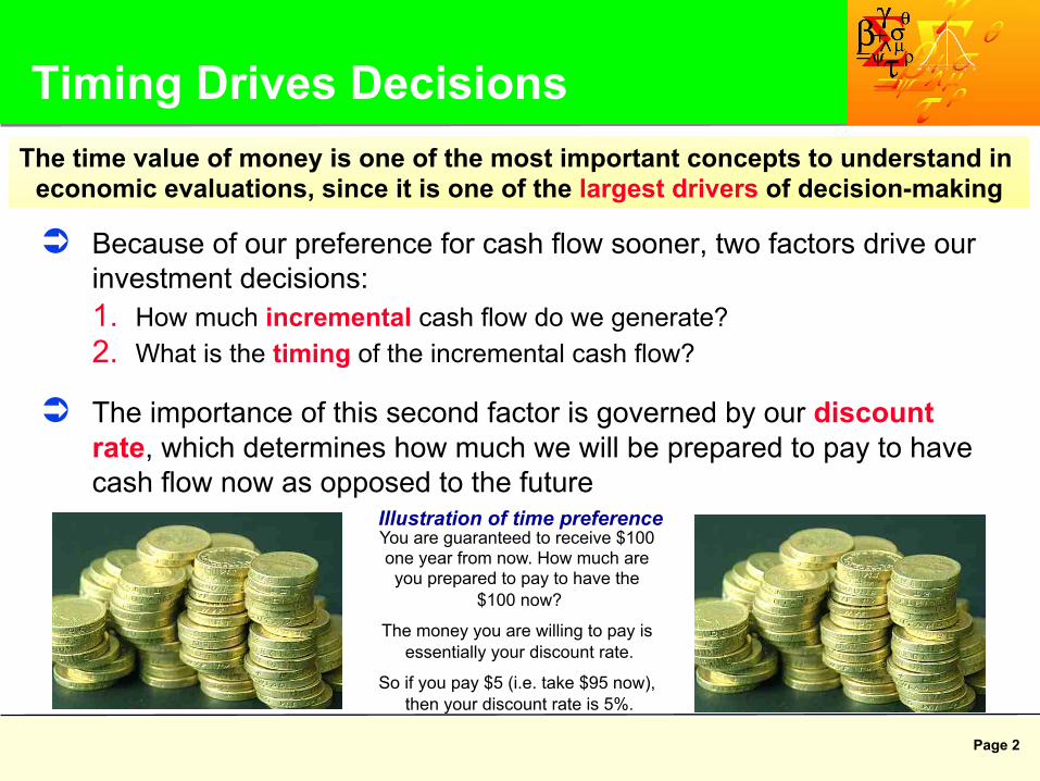
Ü  Because of our preference for cash flow sooner, two factors drive our investment decisions: 1.  How much incremental cash flow do we generate? 2.  What is the timing of the incremental cash flow?

Ü  The importance of this second factor is governed by our discount rate, which determines how much we will be prepared to pay to have cash flow now as opposed to the future

The time value of money is one of the most important concepts to understand in economic evaluations, since it is one of the largest drivers of decision-making

Illustration of time preference You are guaranteed to receive $100 one year from now. How much are you prepared to pay to have the

$100 now?

The money you are willing to pay is essentially your discount rate.

So if you pay $5 (i.e. take $95 now), then your discount rate is 5%.

Page 3

What Determines Discount Rates?

Ü Discount rates are determined by a number of factors: Ü Cost of debt Ü Cost of equity Ü Attitude to risk and uncertainty Ü Returns on current/future portfolio of assets Ü Desired return on investment

Ü Discount rates in the oil industry range from 5% to 15%, with the average around 10%

All oil companies use a discount rate in making investment decisions, but discount rates vary across companies

Page 4

Which Discount Rate?

Ü A commonly used measure of discount rate is the Weighted Average Cost of Capital (WACC)

Ü WACC is a measure of the minimum return a company must earn to satisfy its existing shareholders and creditors

WACC = Cost of Equity x Proportion of Equity in Capital Structure + Cost of Debt x Proportion of Debt in Capital Structure

Page 5

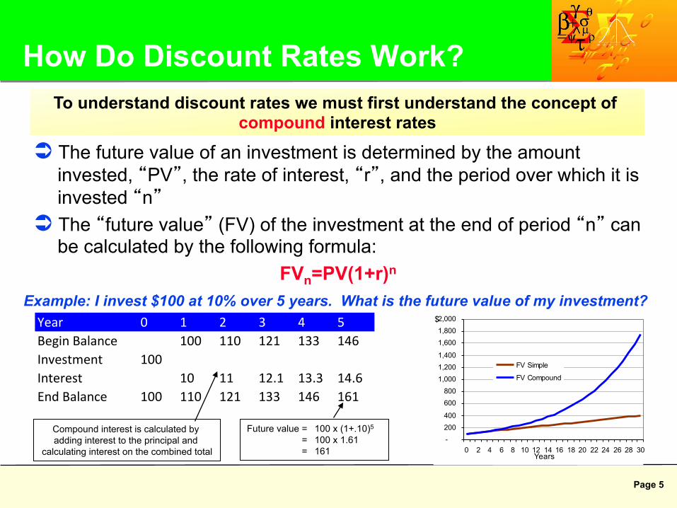
Year 0 1 2 3 4 5Begin  Balance   100 110 121 133 146Investment 100Interest   10 11 12.1 13.3 14.6End  Balance 100 110 121 133 146 161

How Do Discount Rates Work?

Ü The future value of an investment is determined by the amount invested, “PV”, the rate of interest, “r”, and the period over which it is invested “n”

Ü The “future value” (FV) of the investment at the end of period “n” can be calculated by the following formula:

FVn=PV(1+r)n

To understand discount rates we must first understand the concept of compound interest rates

Future value = 100 x (1+.10)5

= 100 x 1.61 = 161

Compound interest is calculated by adding interest to the principal and

calculating interest on the combined total

Example: I invest $100 at 10% over 5 years. What is the future value of my investment?

-200400

600800

1,0001,2001,400

1,6001,8002,000

0 2 4 6 8 10 12 14 16 18 20 22 24 26 28 30Years

$

FV Simple

FV Compound

Page 6

Introducing Discounting

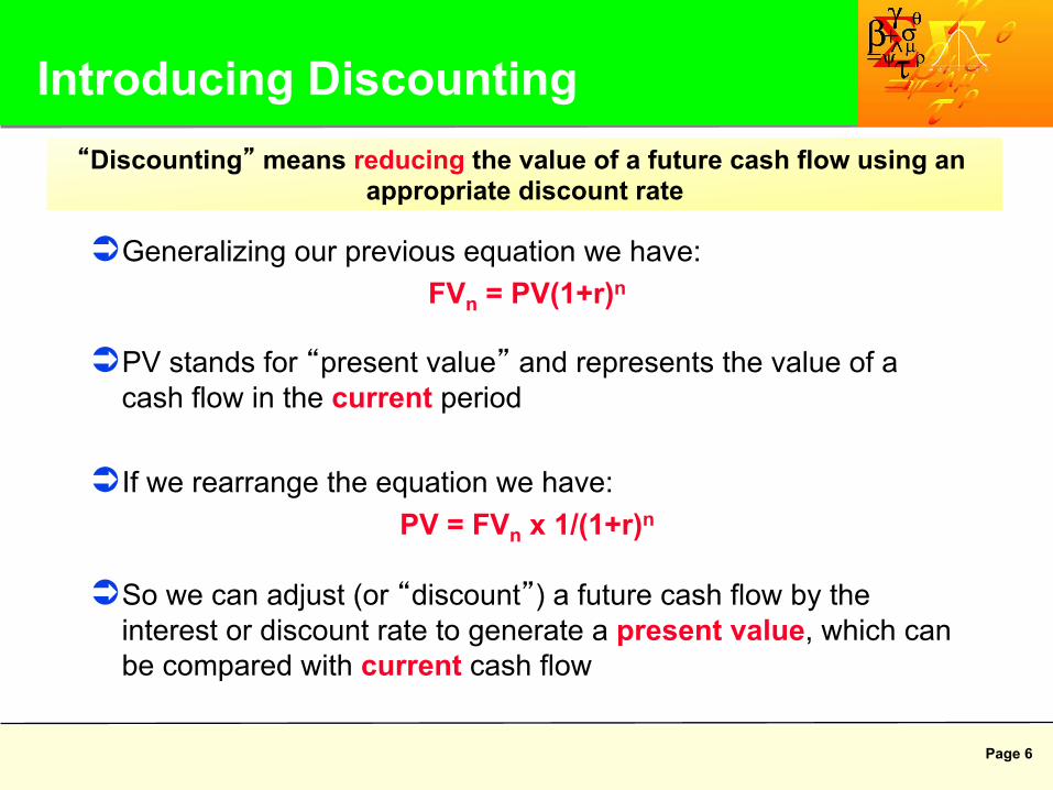
Ü Generalizing our previous equation we have: FVn = PV(1+r)n

Ü PV stands for “present value” and represents the value of a cash flow in the current period

Ü If we rearrange the equation we have: PV = FVn x 1/(1+r)n

Ü So we can adjust (or “discount”) a future cash flow by the interest or discount rate to generate a present value, which can be compared with current cash flow

“Discounting” means reducing the value of a future cash flow using an appropriate discount rate

Page 7

Discounting Example

Example: I can invest money at an interest rate of 8%. Am I better off accepting a cash flow of $100 now or $150 in five years time?

The present value of $150 in five years time:

= $150 / (1+8%)5

= $150 / 1.47

= $102

The present value of $150 in five years has greater value than $100 now so I should accept the $150 in five years

We now have a means of comparing a future cash flow with a current cash flow, given an available interest rate

Page 8

Ü Assuming a series of future cash flows (FVi) the present value (PV) is:

Present Value Present value is the sum of a series of cash flows discounted to a

particular date using an appropriate discount rate

nn

rFV

rFV

rFV

rFVPV

)1(...

)1()1()1( 33

22

11

+++

++

++

+=

The later the cash flow, the smaller the weighting, since the discount factor decreases as we move further out in time

More weight Less weight

Page 9

…therefore the difference between cash flow and discounted cash flow increases

Illustration of Discounting

10% discount rate assumed

As we move further out in time the discount factor decreases…

Page 10

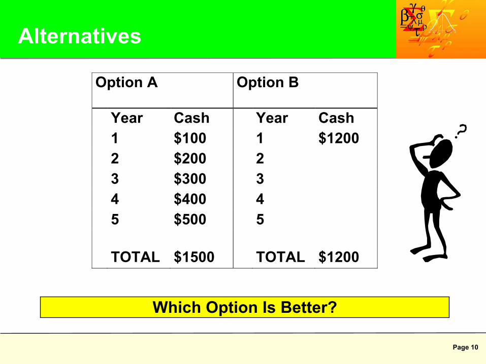
Alternatives

Option A

Option B

Year Cash Year Cash 1 $100 1 $1200 2 $200 2 3 $300 3 4 $400 4 5 $500 5 TOTAL $1500 TOTAL $1200

Which Option Is Better?

Page 11

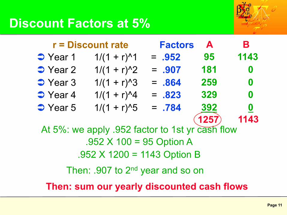
r = Discount rate Factors Ü  Year 1 1/(1 + r)^1 = .952 Ü  Year 2 1/(1 + r)^2 = .907 Ü  Year 3 1/(1 + r)^3 = .864 Ü  Year 4 1/(1 + r)^4 = .823 Ü  Year 5 1/(1 + r)^5 = .784

At 5%: we apply .952 factor to 1st yr cash flow .952 X 100 = 95 Option A

.952 X 1200 = 1143 Option B

Discount Factors at 5%

Then: .907 to 2nd year and so on

Then: sum our yearly discounted cash flows

1257 1143

A B 95 1143 181 0 259 0 329 0 392 0

Page 12

r = Discount rate Factors Ü  Year 1 1/(1 + r)^1 = .870 Ü  Year 2 1/(1 + r)^2 = .756 Ü  Year 3 1/(1 + r)^3 = .658 Ü  Year 4 1/(1 + r)^4 = .572 Ü  Year 5 1/(1 + r)^5 = .497

At 15%: we choose option B WHY?

Discount Factors at 15%

913 1043

A B 87 1043 151 0 197 0 229 0 249 0

Page 13

Ü Our goal as a company is to increase shareholder value

Ü The value metrics and decision criteria help optimize investment decisions that contribute to this goal

Ü Measures are needed to answer two questions: 1. Does the project have economic merit? 2. Which competing project has the most merit?

Ü There is no one single metric that can always answer these questions

Why Do We Need Value Metrics?

Page 14

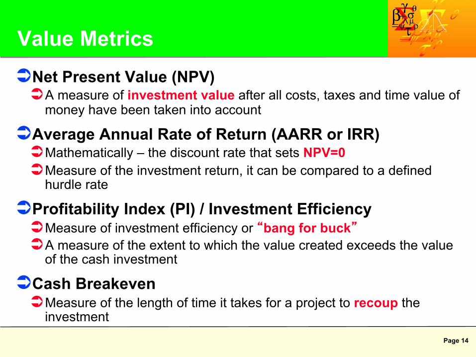
Value Metrics Ü Net Present Value (NPV) Ü A measure of investment value after all costs, taxes and time value of

money have been taken into account

Ü Average Annual Rate of Return (AARR or IRR) Ü Mathematically – the discount rate that sets NPV=0 Ü Measure of the investment return, it can be compared to a defined

hurdle rate

Ü Profitability Index (PI) / Investment Efficiency Ü Measure of investment efficiency or “bang for buck” Ü A measure of the extent to which the value created exceeds the value

of the cash investment

Ü Cash Breakeven Ü Measure of the length of time it takes for a project to recoup the

investment

Page 15

nn

rFV

rFV

rFV

rFVPV

)1(...

)1()1()1( 33

22

11

+++

++

++

+=

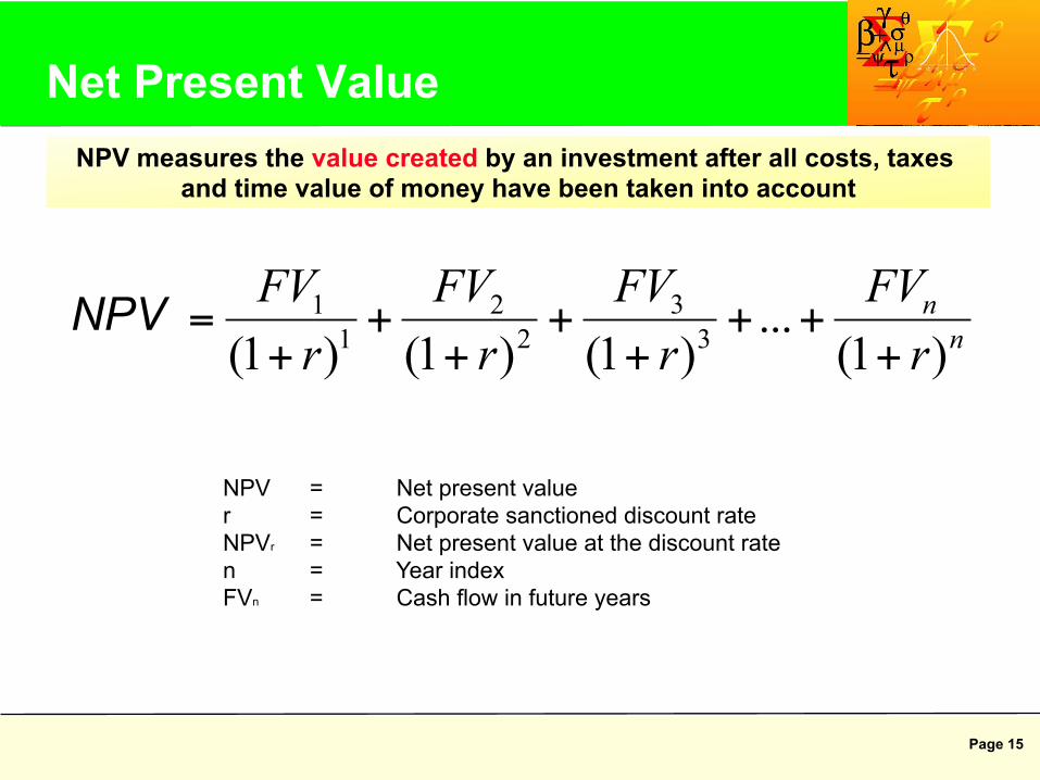
NPV = Net present value r = Corporate sanctioned discount rate NPVr = Net present value at the discount rate n = Year index FVn = Cash flow in future years

Net Present Value NPV measures the value created by an investment after all costs, taxes

and time value of money have been taken into account

NPV

Page 16

Ü NPV is the most commonly used investment appraisal metric

Ü Measures the present value of the cash flows generated by an investment, using a specified discount rate

Ü Attaches greater weighting to earlier cash flows than to later cash flows

Ü Can be used to compare the value generated by all kinds of investments

Net Present Value Decision criterion: projects with NPV greater than zero add value to the

company and should be recommended

Page 17

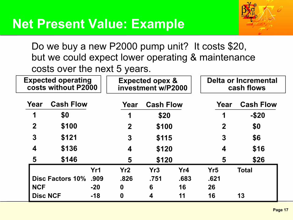
Net Present Value: Example Do we buy a new P2000 pump unit? It costs $20, but we could expect lower operating & maintenance costs over the next 5 years.

Expected operating costs without P2000

Year Cash Flow 1 $0 2 $100 3 $121 4 $136 5 $146

Expected opex & investment w/P2000

Year Cash Flow 1 $20 2 $100 3 $115 4 $120 5 $120

Delta or Incremental cash flows

Year Cash Flow 1 -$20 2 $0 3 $6 4 $16 5 $26 Yr1 Yr2 Yr3 Yr4 Yr5 Total

Disc Factors 10% .909 .826 .751 .683 .621 NCF -20 0 6 16 26 Disc NCF -18 0 4 11 16 13

Page 18

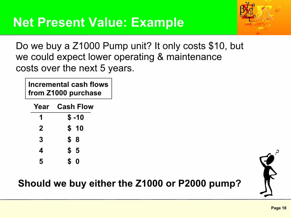
Year Cash Flow 1 $ -10 2 $ 10 3 $ 8 4 $ 5 5 $ 0

Net Present Value: Example

Should we buy either the Z1000 or P2000 pump?

Incremental cash flows from Z1000 purchase

Do we buy a Z1000 Pump unit? It only costs $10, but we could expect lower operating & maintenance costs over the next 5 years.

Year DCF 1 $ -9 2 $ 8 3 $ 6 4 $ 3 5 $ 0

Total is 8

Page 19

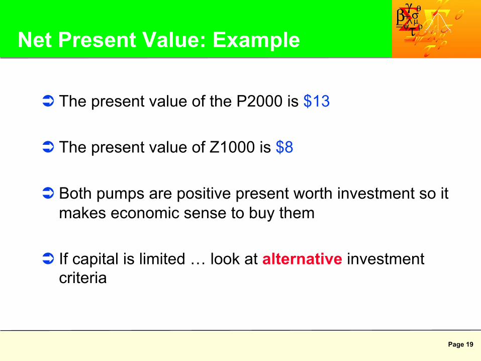
Net Present Value: Example

Ü The present value of the P2000 is $13

Ü The present value of Z1000 is $8

Ü Both pumps are positive present worth investment so it makes economic sense to buy them

Ü  If capital is limited … look at alternative investment criteria

Page 20

Pros and Cons of NPV

Strengths: Ü Shows scale of value generated Ü Works correctly for any type of investment Ü Easily interpreted and universally accepted Ü Can be used to rank projects

Weaknesses: Ü Does not show capital efficiency Ü Discriminates against projects with long-life cash flows Ü Difficult to compare projects of differing magnitudes

Page 21

Average Annual Rate of Return Average annual rate of return (AARR) is the discount rate at which net

present value is equal to zero

AARR here is 30%

Page 22

Annual Average Rate of Return Since inflows of cash occur after the investment period (outflows),

AARR is like a scale to balance the values of the inflows and outflows of cash such that we are indifferent to the investment

NPV(10) = 340

Discount rate = 10%

NPV(20) = 0

Discount rate = 20%

AARR = 20% - the discount rate at which NPV = 0

Outflow

InflowOutflow Inflow

NPV(10) = 340

Discount rate = 10%

NPV(20) = 0

Discount rate = 20%

AARR = 20% - the discount rate at which NPV = 0

Outflow

InflowOutflow Inflow

Page 23

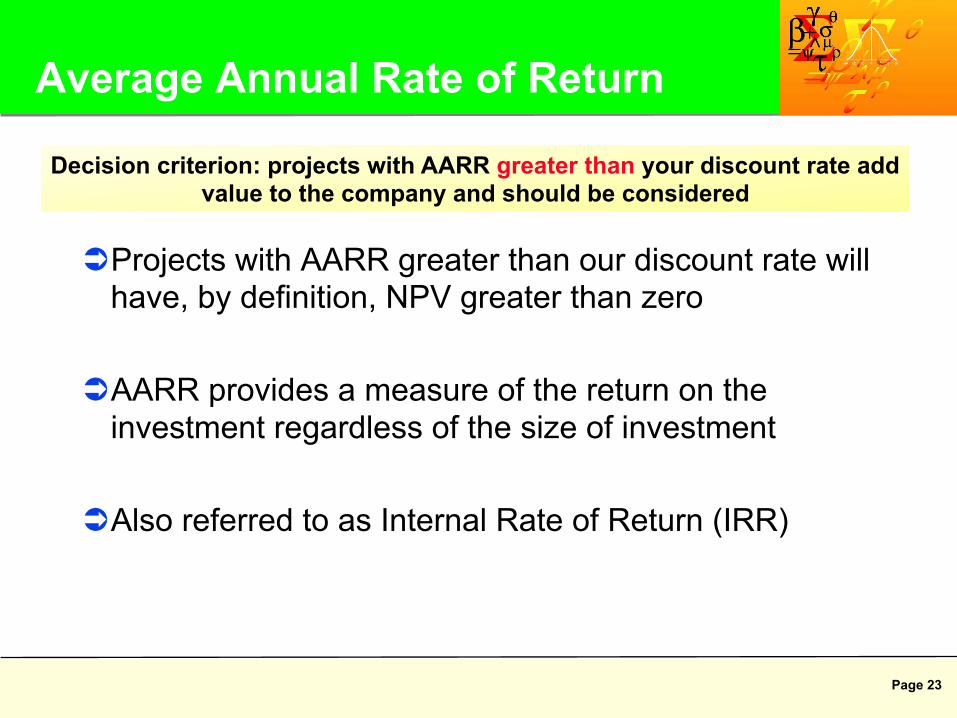
Average Annual Rate of Return

Ü Projects with AARR greater than our discount rate will have, by definition, NPV greater than zero

Ü AARR provides a measure of the return on the investment regardless of the size of investment

Ü Also referred to as Internal Rate of Return (IRR)

Decision criterion: projects with AARR greater than your discount rate add value to the company and should be considered

Page 24

Pros and Cons of AARR

Strengths: Ü  Ties in with NPV Ü  Can be directly compared to a hurdle rate Ü  Allows project comparisons regardless of size

Weaknesses: Ü  Cannot be calculated on cash flows that are all positive or all negative Ü  Ignores project scale Ü  May have multiple solutions

Page 25

Profitability Index (PI) or Investment Efficiency

)()(

CFNegativePVCFPositivePVPI =

Profitability Index measures the efficiency or “bang for buck” of an investment. There are many different versions of investment efficiency.

Profitability index (PI) tells us how many discounted dollars of positive after-tax cash we generate for every dollar of after-tax negative cash flow we invest

It is not a “capital” PI

Absolute value

Page 26

Profitability Index (PI)/Investment Efficiency

Ü Projects with PI greater than one are NPV positive by definition

Ü The same discount rate should be used for the PI calculation as our NPV calculation

Ü We can use the NPV function in Excel to easily calculate PI from our net cash flow

Decision criterion: projects with PI greater than one are NPV positive and should be approved

Page 27

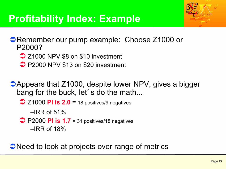
Profitability Index: Example

Ü Remember our pump example: Choose Z1000 or P2000? Ü Z1000 NPV $8 on $10 investment Ü P2000 NPV $13 on $20 investment

Ü Appears that Z1000, despite lower NPV, gives a bigger bang for the buck, let’s do the math... Ü Z1000 PI is 2.0 = 18 positives/9 negatives

– IRR of 51% Ü P2000 PI is 1.7 = 31 positives/18 negatives

– IRR of 18%

Ü Need to look at projects over range of metrics

Page 28

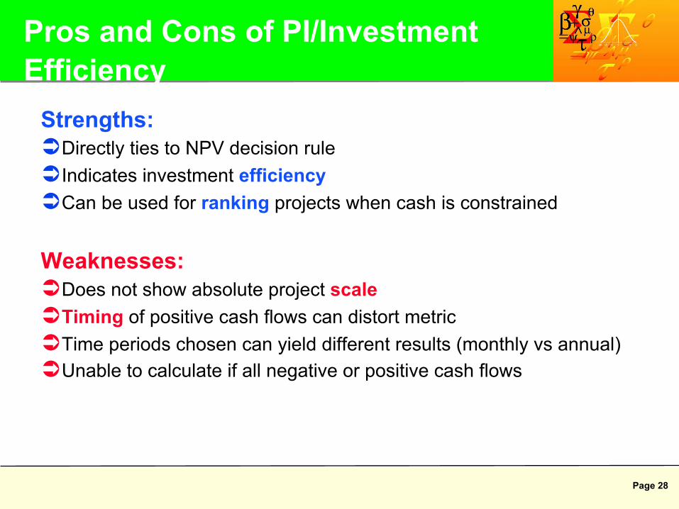
Pros and Cons of PI/Investment Efficiency

Strengths: Ü Directly ties to NPV decision rule Ü Indicates investment efficiency Ü Can be used for ranking projects when cash is constrained

Weaknesses: Ü Does not show absolute project scale Ü Timing of positive cash flows can distort metric Ü Time periods chosen can yield different results (monthly vs annual) Ü Unable to calculate if all negative or positive cash flows

Page 29

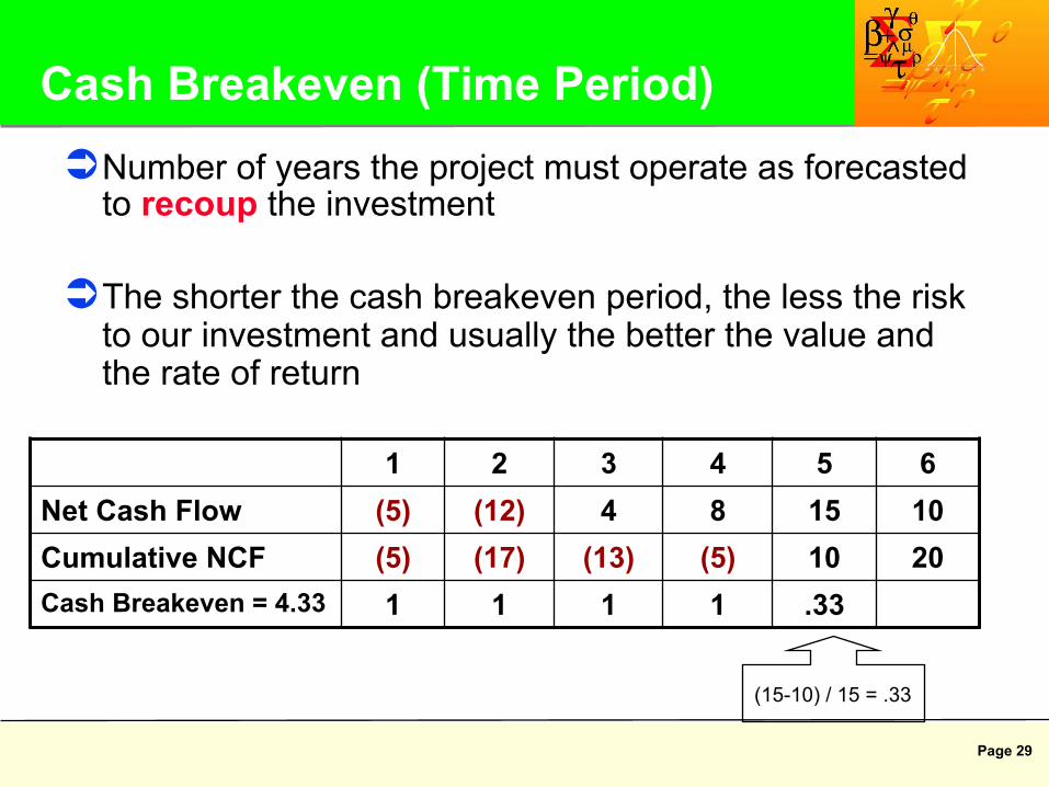
Ü Number of years the project must operate as forecasted to recoup the investment

Ü The shorter the cash breakeven period, the less the risk to our investment and usually the better the value and the rate of return

1 2 3 4 5 6 Net Cash Flow (5) (12) 4 8 15 10 Cumulative NCF (5) (17) (13) (5) 10 20 Cash Breakeven = 4.33 1 1 1 1 .33

Cash Breakeven (Time Period)

(15-10) / 15 = .33

Page 30

Ü Which pump had a better breakeven?

Ü Z1000 had cash flow of -10, +10.... So paid out in two years vs P2000 which took almost 4 years

Cash Breakeven (Time Period)

Page 31

Pros and Cons of Cash Breakeven

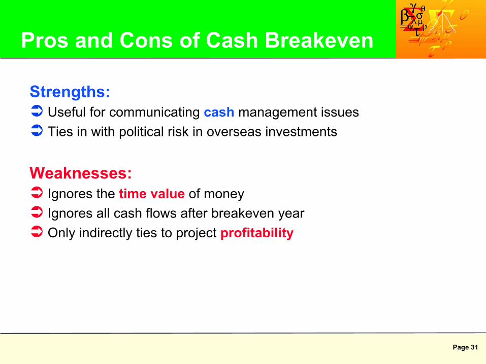
Strengths: Ü Useful for communicating cash management issues Ü Ties in with political risk in overseas investments

Weaknesses: Ü  Ignores the time value of money Ü  Ignores all cash flows after breakeven year Ü Only indirectly ties to project profitability

Page 32

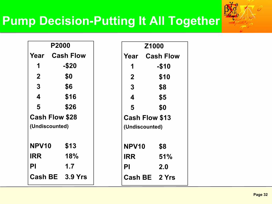
Pump Decision-Putting It All Together

P2000 Year Cash Flow

1 -$20 2 $0 3 $6 4 $16 5 $26

Cash Flow $28 (Undiscounted)

NPV10 $13 IRR 18% PI 1.7 Cash BE 3.9 Yrs

Z1000 Year Cash Flow

1 -$10 2 $10 3 $8 4 $5 5 $0

Cash Flow $13 (Undiscounted)

NPV10 $8 IRR 51% PI 2.0 Cash BE 2 Yrs

Page 33

Agenda

þ Introduction þ Cash Flow þ Time Value of Money/Metrics ý Uncertainty/Tools ¨ Summary

Page 34

Uncertainty

Ü Uncertainty comes from Ü What we know we don't know Ü What we think we know but don't Ü What we don't want to know Ü What we could imagine but don't expect Ü What we can't imagine!

Ü Role in project evaluation and decision making Ü What to do? Ü How to do It?

Page 35

Ü It is difficult to forecast the actual outcomes with a high degree of confidence

Ü However, you can build a logically coherent picture about any given set of outcomes (e.g. high prices, low costs). Ü  You can also discuss the likelihood of these outcomes

Ü You can then talk coherently about these choices: Ü  Alternative ways of carrying out the project Ü  Alternative projects in which ConocoPhillips could invest

Addressing the Uncertainty

Page 36

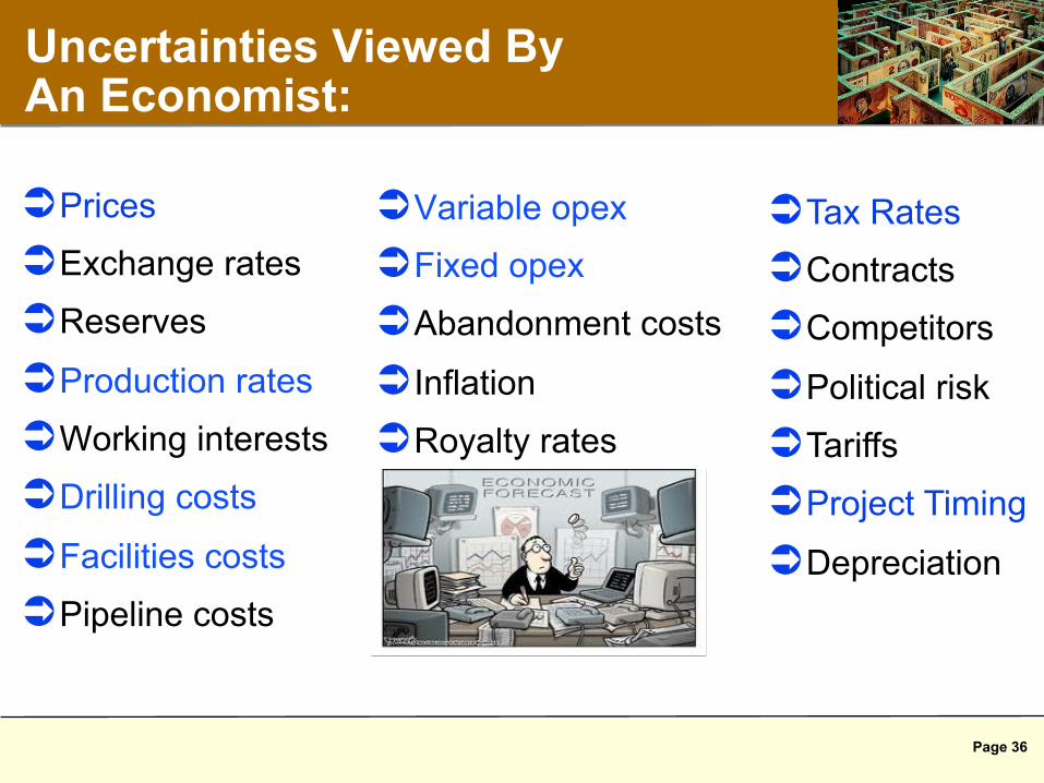
Ü Prices Ü Exchange rates

Ü Reserves

Ü Production rates

Ü Working interests

Ü Drilling costs

Ü Facilities costs

Ü Pipeline costs

Ü Variable opex Ü Fixed opex

Ü Abandonment costs

Ü Inflation

Ü Royalty rates

Uncertainties Viewed By An Economist:

Ü Tax Rates Ü Contracts

Ü Competitors

Ü Political risk

Ü Tariffs

Ü Project Timing

Ü Depreciation

Page 37

Deterministic Economics Ü  Most project analysis begins with a deterministic model

Ü Enter inputs and technical, commercial and fiscal logic to calculate a single outcome

Ü  However, we make no statement about the likelihood of the inputs or the outcome Ü To view alternative results, you need to manually change the

inputs in the model

Ü  Systematically investigating changing the inputs is known as sensitivity analysis Ü Running sensitivities to prices, costs, etc. gives good information

to the decision maker Ü However, ad hoc sensitivities don’t tell you anything about the

likelihood of an outcome

Page 38

CompanyNPV

85%

75%

85%

80%

60%

120%

125%

120%

120%

150%

(200) 0 200 400 600 800

reservesSens

priceSens

capexSens

taxSens

opexSensDownsideUpside

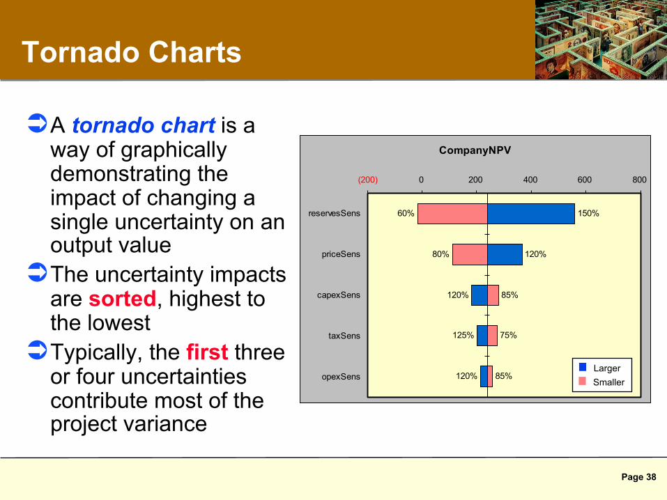
Tornado Charts

Ü A tornado chart is a way of graphically demonstrating the impact of changing a single uncertainty on an output value

Ü The uncertainty impacts are sorted, highest to the lowest

Ü Typically, the first three or four uncertainties contribute most of the project variance

Larger Smaller

Page 39

Probabilistic Economics Ü For more insight, we calculate a result and the

probability that a given result will occur

Ü We then systematically investigate feasible results

Ü We get useful information from the distribution of these results and from various statistical measures

Ü Common techniques used to calculate probabilistic outcomes are: Ü Decision trees Ü Monte Carlo simulation

Page 40

Decision Trees What is a Decision Tree? Ü  A graphical means of

displaying key alternatives and options available via a chronological sequence of decisions and uncertainties

Why create a Decision Tree? Ü It structures the decision

process in an orderly fashion Ü It is a diagnostic tool to map

how outcomes are generated Ü It develops ranges of

outcomes using ranges for input variables

Ü It communicates the decision-making process to management

P90

Drill Field? Reserves Oil Price Net Cash Flow

Time

P10

P50 30% 40%

30%

40%

(218)

P10

30%

(10)

251

P90

P10

P50 30% 40%

30%

217

522

907

P90

P10

P50 30% 40%

30%

798

1233

1780

30%

P50

P90

0

Yes

No

Page 41

Monte Carlo Analysis

Ü In Monte Carlo simulation, the discrete uncertainty inputs are replaced by probability distribution functions

Ü The user then calculates the output over a large number of times (say 1000), and calculates the statistics of the output results (e.g. mean, median, P10 and P90)

Ü Monte Carlo simulations are very useful in giving the likelihood of certain outcomes (e.g. “while positive NPV, this decision has a 60% chance of losing money”)