Embed Size (px)
DESCRIPTION
fddsgdsdf
Citation preview

Land-Ocean Interactions:
Estuarine Circulation
Bob Chant

Land-Ocean Interactions:
Estuarine Circulation Estuary: a semi-enclosed coastal body of water which has a free connection with the open sea and within which sea water is measurably diluted with fresh water derived from land drainage. (Pritchard,1963)
Coastal Ocean
Estuary mouth Estuary
Estuary head
River
Schematic of a typical Estuary

Density gradient
along axis of
estuary
… and in the
vertical (strongly
stratified)
Stratification evolves over time in response to freshwater inflow – shows time scale of estuary residence time can be long

Smaller estuary: salinity shows tidal variability

Characteristics of estuaries • Most estuaries:
– strong tidal forcing – large density difference between river and ocean – complex topography – Long and narrow – can often be approximated by 2-dimensional vertical/along-
axis flow (relatively little across axis flow)
• Mathematically we have equations for salt, mass (volume) and momentum – significant forces: friction (mixing), pressure, nonlinearity, acceleration
(time variability) – typically small: wind, Coriolis, longer that tidal period coastal sea level
(tides are important) – most common dynamic balance is between pressure and friction/mixing
• Mixing affects the salt balance … • … which affects the pressure distribution and pressure gradient
• Can classify estuaries based on their physics (relative magnitude of different terms), or topography/geomorphology

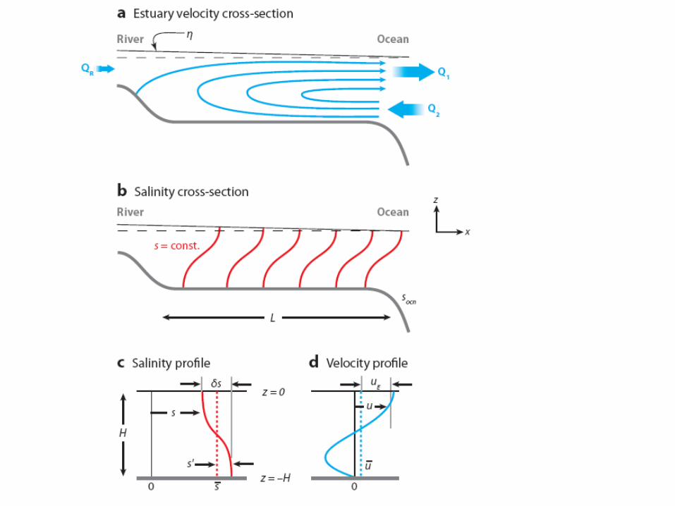
Physics essentials:
• Fresh river water encounters salty ocean water • Fresh = light; salty = heavy • Freshwater flows seaward at the surface • Get landward flow of more dense, salty, water
– estuarine or gravitational or baroclinic circulation – time scales of ~1 day … so Coriolis force is usually of
secondary importance – circulation is evident averaged over a few tidal cycles – mixing and entrainment processes are central to
details of the salt and volume transport balance

Solid– surface Dashed -‐-‐ Bo3om
Current measurements in the Hudson Posi:ve directed Landward
Muh-he-kun-ne-tuk (Mahican name for Hudson—river that flows both ways

km north of the Battery
20 25 30 35 40 45 50 55 60-15
-10
-5
0
m
5 5
5 510
10
10 10
15
20 25 30 35 40 45 50 55 60-15
-10
-5
0
m
5 5510 10
15
20 25 30 35 40 45 50 55 60-15
-10
-5
0
m
55 5
5
1010
1015
20 25 30 35 40 45 50 55 60-20
-10
0
m
55
51015 May 4th
May 6th
May 7th
May 8th
Lower layer (and dye) moving up river against the river flow

River
Ocean
1. No mixing. Zero exchange flow s1=0
so=32
River
Ocean
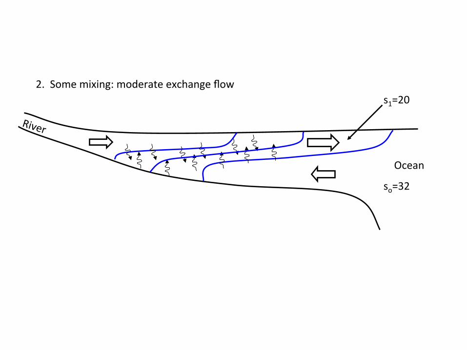
2. Some mixing: moderate exchange flow s1=20
so=32

River
Ocean
Maximal exchange s1=28
so=32
Salt balance on board….
Q1 QR
Qo

Estuarine CirculaFon and Mixing-‐-‐-‐ seemingly counter to the Kundson model But not really!!


Salt field in Hudson During Low River Flow
Neap Fde Exchange flow Dominates And isohalines Slump over Spring Fde Mixing dominates and water column becomes well mixed.
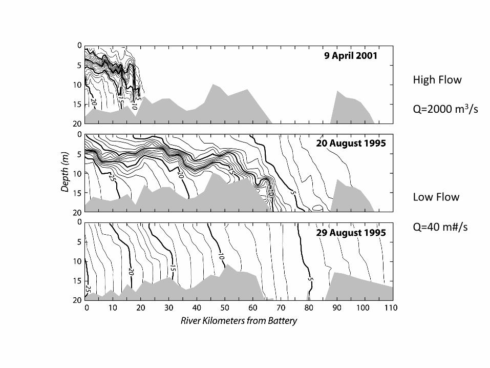
High Flow Q=2000 m3/s Low Flow Q=40 m#/s


Stokes Settling the larger And denser a particle is the faster They fall. Micron-scale particles have (almost) No settling speed mm scale particles may fall at speeds of Mm/s When a whale dies– it falls rapidly to the bottom

1) w=1 mm/s turbulence
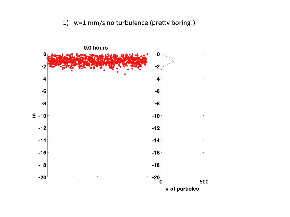
1) w=1 mm/s no turbulence (preXy boring!)
2) w=0 mm/s turbulence
3) w=1 mm/s turbulence

1) w=0 mm/s turbulence

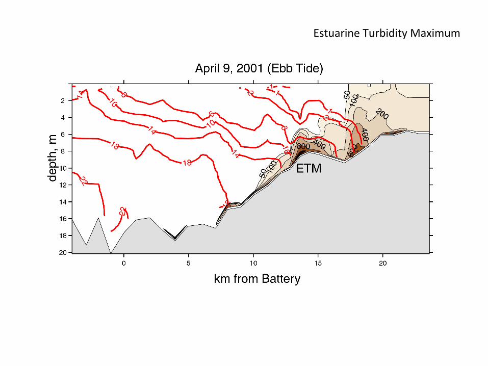
Estuarine Turbidity Maximum

The quesFon of the day: Consider an estuary that is 50 km long, 10m deep and 1 km wide. Moored observaFons at the mouth show that the mean surface to boXom salinity difference is 3 and the mean river flow is 100 m3/s. Use the Knudson model to esFmate the volume transport in the lower layer and the residence Fme of the estuary. Assume that the mean salinity of the ocean water is 30.