6/21/2013

GENERATION OF

NAVIGATION

PARAMETERS IN RINEX

FORMAT FOR IRNSS

SATELLITES By

Nagarji Javed,

Shripad Thakur,

Aditya Singh,

Ayush Gupta

ISRO Summer Internship 2013 Project

Report

1

Declaration

We declare that this written submission represents our ideas in our own words and

where others ideas or words have been included, we have adequately cited and

referenced the original sources. We also declare that we have adhered to all

principles of academic honesty and integrity and have not misrepresented or

fabricated or falsified data/idea/fact/source in our submission. We understand that

any violation of the above will be cause of disciplinary action by the institute and

can also evoke penal action from the sources which have thus not been properly

cited or from whom proper permission has not been taken when needed.

By

Nagarji Javed,

Shripad Thakur,

Aditya Singh,

Ayush Gupta

2

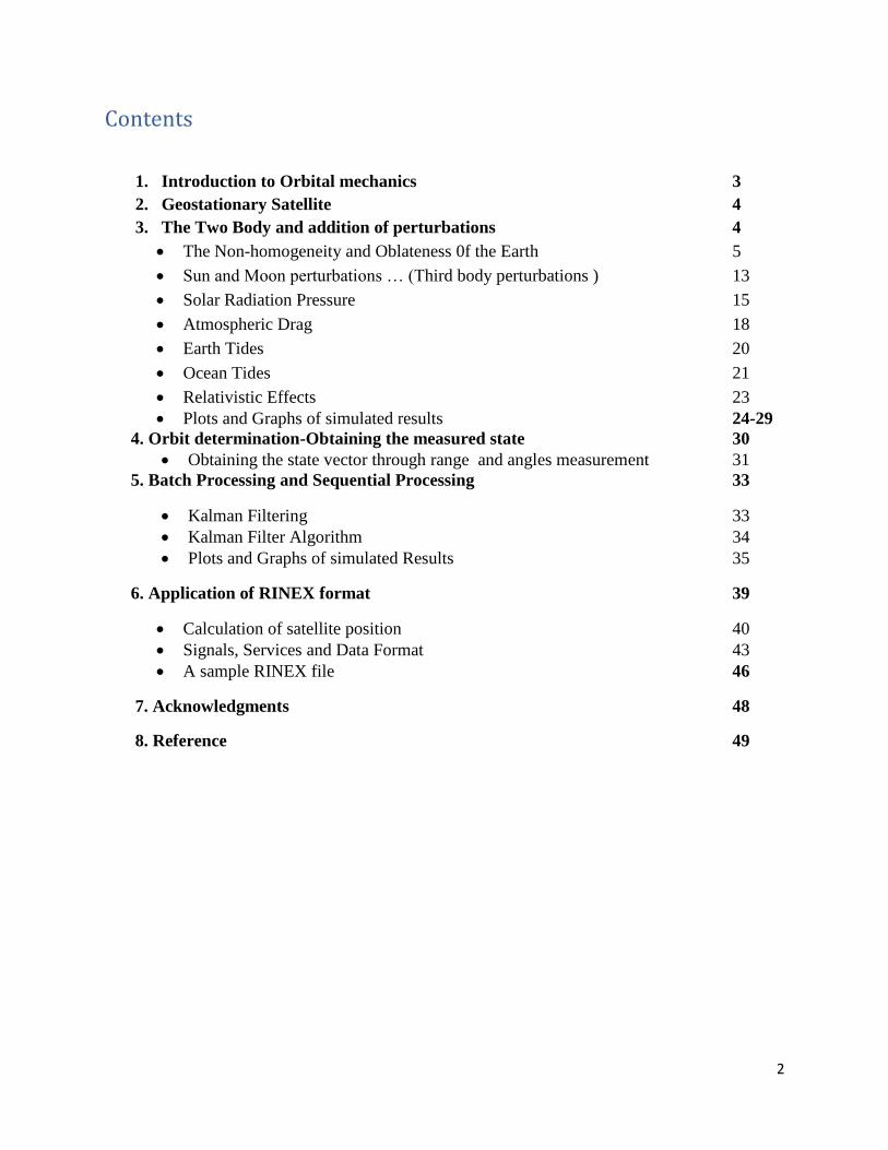
Contents

1. Introduction to Orbital mechanics 3

2. Geostationary Satellite 4

3. The Two Body and addition of perturbations 4

The Non-homogeneity and Oblateness 0f the Earth 5

Sun and Moon perturbations … (Third body perturbations ) 13

Solar Radiation Pressure 15

Atmospheric Drag 18

Earth Tides 20

Ocean Tides 21

Relativistic Effects 23

Plots and Graphs of simulated results 24-29

4. Orbit determination-Obtaining the measured state 30

Obtaining the state vector through range and angles measurement 31

5. Batch Processing and Sequential Processing 33

Kalman Filtering 33

Kalman Filter Algorithm 34

Plots and Graphs of simulated Results 35

6. Application of RINEX format 39

Calculation of satellite position 40

Signals, Services and Data Format 43

A sample RINEX file 46

7. Acknowledgments 48

8. Reference 49

3

Orbital mechanics, as applied to artificial spacecraft, is based on celestial mechanics. In

studying the motion of satellites, quite elementary principles are necessary. Kepler provided

three basic empirical laws that describe motion in unperturbed planetary orbits. Newton

formulated the more general physical laws governing the motion of a planet, laws that were

consistent with Kepler's observations. In this report, ideal, unperturbed Keplerian orbits will be

seen briefly and the dynamical equations of motion for realistic, perturbed orbits - will be

analyzed. Kepler's laws of motion describe ideal orbits that do not exist in nature. Perturbing

forces and physical anomalies cause spacecraft orbits to have strange properties; in most cases

these cause difficulties for the space control engineer, but in other cases these properties may be

of enormous help.

Kepler provided three empirical laws for planetary motion, based on Brahe's

Planetary observations.

1. The orbit of each planet is an ellipse with the sun located at one focus.

2. The radius vector drawn from the sun to any planet sweeps out equal areas in equal time

intervals (the law of areas).

3. Planetary periods of revolution are proportional to the [mean distance to sun]3/2

Newton stated in his law of gravitation that any two particles attract each other with a force

given by the expression 𝐹 = 𝐺𝑚1𝑚2

𝑟3 𝒓

where r is a vector of magnitude r along the line connecting the two particles with masses m1 and

m2 and G = 6.669 X 10-11 m3/kg-s2 is the universal constant of gravitation. This is the famous

inverse square law of force.

The two-body problem is an idealized situation in which only two bodies exist that are in relative

motion in a force field described by the inverse square law. In order to obtain simple analytical

results for the motion of celestial bodies or spacecraft, it is assumed that additional bodies are

situated far enough from the two-body system, thus no appreciable force is exerted on them from

a third body.

For a mass of unity we find that 𝑑ℎ

𝑑𝑡 = 0 and h = r x v = const. The vector h is called the specific

angular momentum. It is perpendicular to both r and v, and is also constant in space. This means

that the motion of the particle takes place in a plane.

There are several parameters that represent the orbital motion in a plane. The physical

parameters sufficient to define an orbit are its total energy E and its momentum h. The geometric

parameters sufficient to define the orbit are the semi-major axis a and the eccentricity e. The

mean anomaly M enables finding the location of the moving body in the orbit with time. There

are three more parameters are necessary to define an orbit in space.

The angle between the plane of revolution of the particle around earth and the X-Y plane - which

is also the equatorial plane of the earth ( since all measurements are in the eci coordinate system)

is an angle i, the inclination of the orbit. The orbital plane and the equatorial plane intersect at the

node line. The angle in the equator plane that separates the node line from the X axis is called the

right ascension, Ω. In the orbit plane, r is the radius vector to the moving body; rp is the radius

vector to the perigee of the orbit from the focus of the orbit. The angle between rp and the node

line is 𝜔, the argument of perigee. These three parameters, together with the three parameters (a,

4

e, and M) of the orbit in the plane, complete a system of six parameters that suffices to define the

location in space of a body moving in any Keplerian orbit. These parameters are known as the

classical orbit parameters, which are redefined as follows:

1. Semi-major axis, a

2. Eccentricity, e

3. Inclination angle, i

4. Argument of perigee, 𝜔

5. Right ascension of the ascending node, Ω

6. Mean anomaly, M = n( t-t0)

GEOSTATIONARY SATELLITE

A geostationary satellite moves under the gravitational force of the earth. Ideally it is a two body

system where the satellite revolves around the earth in an elliptical orbit . Since the eccentricity

of the orbit is very small (around 0.00045) it can be assumed as a near circular orbit. Also the

inclination of an ideal geostationary satellite is zero degrees but in real cases it is a very small

non zero value.

Ideal Keplerian orbits were treated under the basic assumptions that the motion of a body in

these orbits is a result of just the gravitational attraction between two bodies. This ideal situation

does not exist in practice. The two-body problem of motion is an idealization, and additional

forces acting on any moving body must be taken into account. The perturbing forces are both

conservative and non-conservative in nature. The perturbing forces caused by the additional

bodies are conservative field forces. In the case of geostationary satellites which are high-orbit

satellites, the effects of the conservative perturbing forces of the sun and the moon on the motion

of the satellite cannot be ignored.

In general the perturbing forces are due to these following reasons:

1. Non-homogeneity and Oblateness 0f the Earth

2. A third body gravitational force

3. Solar radiation pressure of the sun

4. Atmospheric drag

5. Infrared radiations from earth

6. Earth’s albedo

7. Relativistic effect due to earth

8. Solid tides

Geostationary satellites are high-altitude satellites so they do not experience atmospheric drag as

this drag force is only encountered by low-orbit satellites. Forces 1-3 are major contributors to

the satellite orbit position and velocity so they will be dealt with first, while 5-8 are minor forces

which have very little effect (order of magnitude 4-5 less than major ones) so they will be dealt

with later.

5

The Non-homogeneity and Oblateness 0f the Earth

(reference no. 1,3 and 7)

One of the most important perturbing forces on earth-orbiting satellites arises from the non-

homogeneity of the earth. The earth globe is not a perfect sphere, and neither is its mass

distribution homogeneous. These physical facts produce perturbing accelerations on the moving

body. The consequences of these accelerations are variations of the orbital parameters of earth-

orbiting satellites.

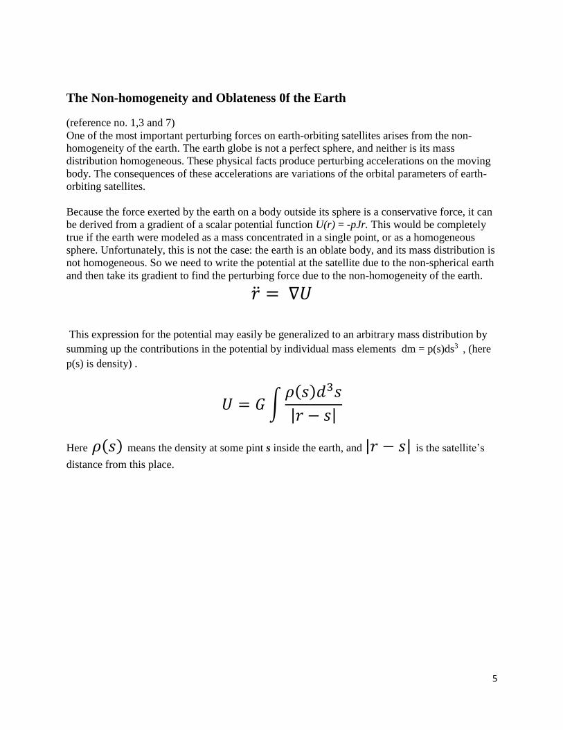
Because the force exerted by the earth on a body outside its sphere is a conservative force, it can

be derived from a gradient of a scalar potential function U(r) = -pJr. This would be completely

true if the earth were modeled as a mass concentrated in a single point, or as a homogeneous

sphere. Unfortunately, this is not the case: the earth is an oblate body, and its mass distribution is

not homogeneous. So we need to write the potential at the satellite due to the non-spherical earth

and then take its gradient to find the perturbing force due to the non-homogeneity of the earth.

= ∇𝑈

This expression for the potential may easily be generalized to an arbitrary mass distribution by

summing up the contributions in the potential by individual mass elements dm = p(s)ds3 , (here

p(s) is density) .

𝑈 = 𝐺 ∫𝜌(𝑠)𝑑3𝑠

|𝑟 − 𝑠|

Here 𝜌(𝑠) means the density at some pint s inside the earth, and |𝑟 − 𝑠| is the satellite’s

distance from this place.

6

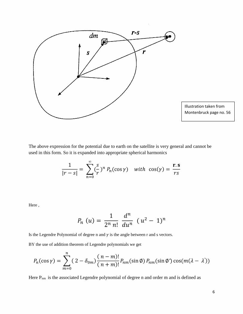
The above expression for the potential due to earth on the satellite is very general and cannot be

used in this form. So it is expanded into appropriate spherical harmonics

1

|𝑟 − 𝑠|= ∑(

𝑠

𝑟 )𝑛 𝑃𝑛(cos 𝛾)

∞

𝑛=0

𝑤𝑖𝑡ℎ cos(𝛾) = 𝐫. 𝐬

𝑟𝑠

Here ,

𝑃𝑛 (𝑢) = 1

2𝑛 𝑛!

𝑑𝑛

𝑑𝑢𝑛 ( 𝑢2 − 1)𝑛

Is the Legendre Polynomial of degree n and 𝛾 is the angle between r and s vectors.

BY the use of addition theorem of Legendre polynomials we get

𝑃𝑛(cos 𝛾) = ∑ ( 2 − 𝛿0𝑚)( 𝑛 − 𝑚)!

( 𝑛 + 𝑚)!𝑃𝑛𝑚(sin ∅) 𝑃𝑛𝑚(sin ∅′) cos(𝑚(𝜆 − 𝜆′))

𝑛

𝑚=0

Here Pnm is the associated Legendre polynomial of degree n and order m and is defined as

Illustration taken from

Montenbruck page no. 56

7

𝑃𝑛𝑚 (𝑢) = ( 1 − 𝑢2)𝑚/2 𝑑𝑚

𝑑𝑢𝑚𝑃𝑛(𝑢)

one can write earth’s gravitational potential in the form, (Montenbruck chapter 3)

𝑈 = 𝐺𝑀

𝑟∑ ∑

𝑅𝑛

𝑟𝑛𝑃𝑛𝑚(sin ∅)(𝐶𝑛𝑚 cos(𝑚𝜆) + 𝑆𝑛𝑚 sin(𝑚𝜆))

𝑛

𝑚=0

.

∞

𝑛=0

with coefficients

𝐶𝑛𝑚 = 2 − 𝛿0𝑚

𝑀 (𝑛 − 𝑚)!

( 𝑛 + 𝑚)!∫

𝑠𝑛

𝑅𝑛 𝑃𝑛𝑚(sin ∅′) cos(𝑚𝜆′) 𝜌(𝑠)𝑑3𝑠

𝑆𝑛𝑚 = 2 − 𝛿0𝑚

𝑀 (𝑛 − 𝑚)!

( 𝑛 + 𝑚)!∫

𝑠𝑛

𝑅𝑛 𝑃𝑛𝑚(sin ∅′) sin(𝑚𝜆′) 𝜌(𝑠)𝑑3𝑠

These geopotential coefficients describe the dependence of the potential on earth’s internal mass

distribution.

The harmonics can be divided into 3 groups:

Zonal harmonics

Sectorial harmonics

Tesseral harmonics

Zonal harmonics are the harmonics that are symmetric about the earth rotation axis. They have

only latitude dependence and not on the longitude. The coefficients with m=0 are called zonal

Table copied from

Montenbruck page no. 57

8

coefficients because they are not dependant on longitude. Legendre polynomial with m=0 only

have sine terms.

Sectorial harmonics are a function of longitude only. The coefficients with m=n are called

sectorial coefficients because of their latitude independence. Legendre polynomial with m=n

only have cosine terms.

Tesseral harmonics are dependent on both longitude and latitude. The coefficients with m>0

and m<n are tesseral coefficients. Legendre polynomial with m=0 only have both sine and

cosine terms.

The net effects of these perturbations are periodic but short term changes in semi major axis,

eccentricity and inclination angle but these changes do not show in the long run and their average

value remains constant. . Since the earth is neither a perfect sphere nor a perfect ellipse, every

time the satellite crosses the perigee its velocity is greater than expected at that point which

means it is more closer to earth than expected and every time it reaches its apogee its speed is

less than expected at that point which means it is more farther to earth than expected. This

happens in every revolution which is responsible for the periodic changes in e and a even though

their mean remains same for a long time interval. The zonal harmonics are responsible for a very

small shift in inclination angle also. The earth can be modeled as a sphere with an extra bulge at

the equator with additional radius of 20 km. A geostationary satellite ideally should be exactly at

the equator all the time but in reality its latitude may vary about 0 degree by 0.1 degrees. So

whenever our geostationary satellite is slightly above 0 degrees a component of the force from

the extra bulge will attract it downwards causing the angular momentum of the satellite to shift

because of the torque produced by the force due to this extra bulge is in east direction. Now

when the satellite is below 0 degrees then the bulge will have an upward force and this will cause

a torque in west direction. This happens in every revolution. The important thing here is that this

torque is because of the tangential component of the extra force due to bulge. So now we have a

rough idea that the inclination changes are due to the tangential forces exerted by the bulge while

the variation in apogee is due to radial components.

The tesseral and sectorial terms cause the forces in direction tangential to the longitudes which

causes longitude acceleration. This acceleration depends on the longitude we are on. Writing the

potential due to these terms and taking its gradient with respect to the longitude gives and

expression for the longitudinal acceleration. This gradient shows that the force is zero at 4

longitudes: two stable and twp unstable equilibrium points. Our geostationary satellite is at a

stable longitude at about 74 degrees east over Bhopal.

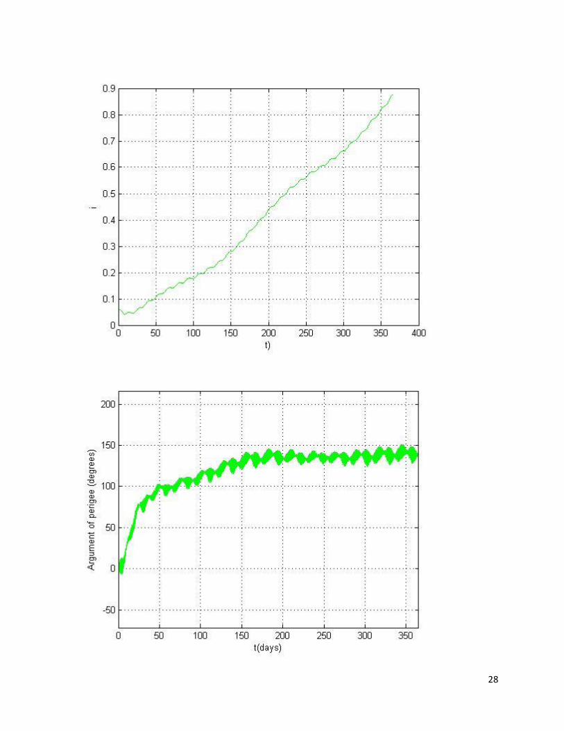
But on the other hand the effects on RAAN, argument of perigee and mean anomaly are secular

i.e. they are significant in the long term analysis. This is because the earth’s geopotential changes

the RAAN which in turn changes the other two parameters

(Re is taken as the mean radius of the earth at equator.)

9

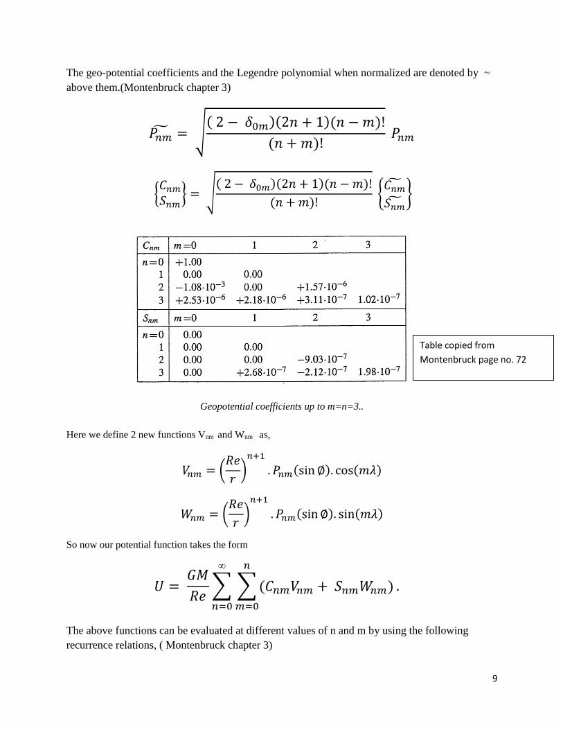
The geo-potential coefficients and the Legendre polynomial when normalized are denoted by ~

above them.(Montenbruck chapter 3)

𝑃𝑛 = √( 2 − 𝛿0𝑚)(2𝑛 + 1)(𝑛 − 𝑚)!

(𝑛 + 𝑚)! 𝑃𝑛𝑚

𝐶𝑛𝑚

𝑆𝑛𝑚 = √

( 2 − 𝛿0𝑚)(2𝑛 + 1)(𝑛 − 𝑚)!

(𝑛 + 𝑚)!

𝐶𝑛

𝑆𝑛

Geopotential coefficients up to m=n=3..

Here we define 2 new functions Vnm and Wnm as,

𝑉𝑛𝑚 = (𝑅𝑒

𝑟)

𝑛+1

. 𝑃𝑛𝑚(sin ∅). cos(𝑚𝜆)

𝑊𝑛𝑚 = (𝑅𝑒

𝑟)

𝑛+1

. 𝑃𝑛𝑚(sin ∅). sin(𝑚𝜆)

So now our potential function takes the form

𝑈 = 𝐺𝑀

𝑅𝑒∑ ∑ (𝐶𝑛𝑚𝑉𝑛𝑚 + 𝑆𝑛𝑚𝑊𝑛𝑚)

𝑛

𝑚=0

.

∞

𝑛=0

The above functions can be evaluated at different values of n and m by using the following

recurrence relations, ( Montenbruck chapter 3)

Table copied from

Montenbruck page no. 72

10

𝑉𝑛𝑚 = (2𝑚 − 1) 𝑥𝑅𝑒

𝑟2𝑉𝑚−1,𝑚−1 −

𝑦𝑅𝑒

𝑟2𝑊𝑚−1,𝑚−1

𝑊𝑛𝑚 = (2𝑚 − 1) 𝑥𝑅𝑒

𝑟2𝑊𝑚−1,𝑚−1 +

𝑦𝑅𝑒

𝑟2𝑉𝑚−1,𝑚−1

and

𝑉𝑛𝑚 = (2𝑛 − 1

𝑛 − 𝑚) .

𝑧𝑅𝑒

𝑟2 . 𝑉𝑛−1,𝑚 − (

𝑛 + 𝑚 − 1

𝑛 − 𝑚) .

𝑅𝑒2

𝑟2. 𝑉𝑛−2,𝑚

𝑊𝑛𝑚 = (2𝑛 − 1

𝑛 − 𝑚) .

𝑧𝑅𝑒

𝑟2 . 𝑊𝑛−1,𝑚 − (

𝑛 + 𝑚 − 1

𝑛 − 𝑚) .

𝑅𝑒2

𝑟2. 𝑊𝑛−2,𝑚

𝑉00 = 𝑅𝑒

𝑟 𝑎𝑛𝑑 𝑊00 = 0

The acceleration can be directly calculated from the expression given in Montenbruck page no.

68.

If m = 0 then

𝑥𝑛0 = 𝐺𝑀

𝑅𝑒2. −𝐶𝑛0𝑉𝑛+1,1

𝑦𝑛0 = 𝐺𝑀

𝑅𝑒2. −𝐶𝑛0𝑊𝑛+1,1

Else when 0<m <n

𝑥𝑛𝑚 = 𝐺𝑀

𝑅𝑒2.1

2. (−𝐶𝑛𝑚𝑉𝑛+1,𝑚+1 − 𝑆𝑛𝑚𝑊𝑛+1,𝑚+1)

+ (𝑛 − 𝑚 + 2)!

(𝑛 − 𝑚)! . (𝐶𝑛𝑚𝑉𝑛+1,𝑚−1 + 𝑆𝑛𝑚𝑊𝑛+1,𝑚−1)

𝑦𝑛𝑚 = 𝐺𝑀

𝑅𝑒2.1

2. (−𝐶𝑛𝑚𝑊𝑛+1,𝑚+1 + 𝑆𝑛𝑚𝑉𝑛+1,𝑚+1)

+ (𝑛 − 𝑚 + 2)!

(𝑛 − 𝑚)! . (−𝐶𝑛𝑚𝑊𝑛+1,𝑚−1 + 𝑆𝑛𝑚𝑉𝑛+1,𝑚−1)

11

𝑧𝑛𝑚 = 𝐺𝑀

𝑅𝑒2( 𝑛 − 𝑚 + 1). (−𝐶𝑛𝑚𝑉𝑛+1,𝑚 − 𝑆𝑛𝑚𝑊𝑛+1,𝑚)

The above formulae are given in r = r(x,y,z) where x ,y and z are in e.c.e.f. (earth fixed )

coordinates so we need to convert these coordinated into e.c.i coordinates to get accelerations in

inertial frame.

All the values of Legendre polynomials were taken and verified from Vallado chapter on special

perturbation methods.

CODE

Converting ECI Coordinated To ECEF And Then Calculating The Latitude And

Longitude Of The Satellite

ecef= [ cos(hh) sin(hh) 0 ; -sin(hh) cos(hh) 0 ; 0 0 1]*[X2-X1 Y2-Y1 Z2-Z1]';

glong2=atan2(ecef(2),ecef(1));

% longitude of the satellite

lat2 = atan2((Z2-Z1),(norm(X2-X1,Y2-Y1)));

% latitude of the satellite

% coefficients Vnm and Wnm ( referred from MONTENBRUCK)

V33 = (Re/r)^4*15*(cos(lat2))^3*cos(3*glong2);

W33 = (Re/r)^4*15*(cos(lat2))^3*sin(3*glong2);

V32 = (Re/r)^4*15*sin(lat2)*(cos(lat2))^2*cos(2*glong2);

W32 = (Re/r)^4*15*sin(lat2)*(cos(lat2))^2*sin(2*glong2);

V31 = (Re/r)^4*(cos(lat2))*((15*(sin(lat2))^2 - 3)/2)*cos(glong2);

W31 = (Re/r)^4*(cos(lat2))*((15*(sin(lat2))^2 - 3)/2)*sin(glong2);

V30 = (5/6)*ecef(3)*(Re^4/r^5)*(3*(sin(lat2))^2 -1) - (2/3)*((Re/r)^4)*sin(lat2);

W30 = 0;

V42 = (105/2)*(ecef(3))*(Re^5/r^6)*sin(lat2)*(cos(lat2))^2*cos(2*glong2) - (15/2)*(Re/r)^5 *

(cos(lat2))^2 * cos(2*glong2);

12

W42 = (105/2)*(ecef(3))*(Re^5/r^6)*sin(lat2)*(cos(lat2))^2*sin(2*glong2) - (15/2)*(Re/r)^5 *

(cos(lat2))^2 * sin(2*glong2);

V41 = (7/2)*(ecef(3))*(Re^5/r^6)*cos(lat2)*(5*(sin(lat2))^2-1)*cos(glong2) - (4)*(Re/r)^5 *

cos(lat2) * sin(lat2) * cos(glong2);

W41 = (7/2)*(ecef(3))*(Re^5/r^6)*cos(lat2)*(5*(sin(lat2))^2-1)*sin(glong2) - (4)*(Re/r)^5 *

cos(lat2) * sin(lat2) * sin(glong2);

V40 = (Re/r)^5*(3*(sin(lat2))^2 - 1)*((35/24)*((ecef(3))/r)^2 - 3/8) -

(7/6)*(ecef(3))*(Re^5/r^6)*sin(lat2);

W40 = 0;

V43 = 105*(ecef(3))*(Re^5/r^6)*(cos(lat2))^3*cos(3*glong2) ;

W43 = 105*(ecef(3))*(Re^5/r^6)*(cos(lat2))^3*sin(3*glong2) ;

V44 = 105*(Re^5/r^6)*((cos(lat2))^3)*((ecef(1))*cos(3*glong2) - (ecef(2))*sin(3*glong2));

W44 = 105*(Re^5/r^6)*((cos(lat2))^3)*((ecef(1))*sin(3*glong2) + (ecef(2))*cos(3*glong2));

Acceleration terms from various harmonics

%% all accelerations due to geopotential changes are taken from montenbruck

% acc due to zonal term n=2,m=0

AXz1 = ( G*m1/Re^2 )*( - C20*V31 ) ;

AYz1 = ( G*m1/Re^2 )*( - C20*W31 ) ;

AZz1 = ( G*m1/Re^2 )*(3*( -C20*V30 - S20*W30) ) ;

%for SECTORAL harmonic effect due to n=2, m=2

%

AXs1 = ( G*m1/Re^2 )*(1/2)*(( -C22*V33- S22*W33 )+2*( C22*V31+S22*W31 )) ;

AYs1 = ( G*m1/Re^2 )*(1/2)*(( -C22*W33+ S22*V33 )+2*( -C22*W31- S22*V31 )) ;

AZs1 = ( G*m1/Re^2 )*(1)*( -C22*V32- S22*W32 ) ;

% acc due to zonal term n=3, m=0

%

AXz2 = ( G*m1/Re^2 )*( - C30*V41 ) ;

AYz2 = ( G*m1/Re^2 )*( - C30*W41 ) ;

13

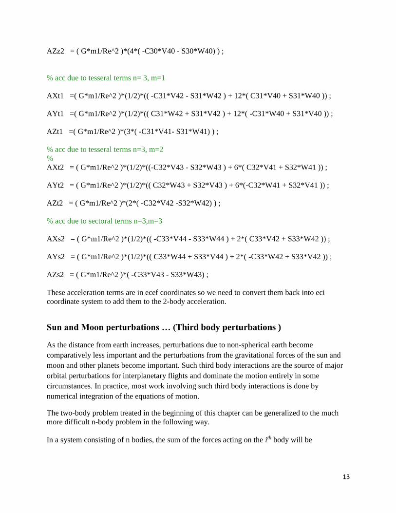
AZz2 = ( G*m1/Re^2 )*(4*( -C30*V40 - S30*W40) ) ;

% acc due to tesseral terms n= 3, m=1

AXt1 =( G*m1/Re^2 )*(1/2)*(( -C31*V42 - S31*W42 ) + 12*( C31*V40 + S31*W40 )) ;

AYt1 =( G*m1/Re^2 )*(1/2)*(( C31*W42 + S31*V42 ) + 12*( -C31*W40 + S31*V40 )) ;

AZt1 =( G*m1/Re^2 )*(3*( -C31*V41- S31*W41) ) ;

% acc due to tesseral terms n=3, m=2

%

AXt2 = ( G*m1/Re^2 )*(1/2)*((-C32*V43 - S32*W43 ) + 6*( C32*V41 + S32*W41 )) ;

AYt2 = ( G*m1/Re^2 )*(1/2)*(( C32*W43 + S32*V43 ) + 6*(-C32*W41 + S32*V41 )) ;

AZt2 = ( G*m1/Re^2 )*(2*( -C32*V42 -S32*W42) ) ;

% acc due to sectoral terms n=3,m=3

AXs2 = ( G*m1/Re^2 )*(1/2)*(( -C33*V44 - S33*W44 ) + 2*( C33*V42 + S33*W42 )) ;

AYs2 = ( G*m1/Re^2 )*(1/2)*(( C33*W44 + S33*V44 ) + 2*( -C33*W42 + S33*V42 )) ;

AZs2 = ( G*m1/Re^2 )*( -C33*V43 - S33*W43) ;

These acceleration terms are in ecef coordinates so we need to convert them back into eci

coordinate system to add them to the 2-body acceleration.

Sun and Moon perturbations … (Third body perturbations )

As the distance from earth increases, perturbations due to non-spherical earth become

comparatively less important and the perturbations from the gravitational forces of the sun and

moon and other planets become important. Such third body interactions are the source of major

orbital perturbations for interplanetary flights and dominate the motion entirely in some

circumstances. In practice, most work involving such third body interactions is done by

numerical integration of the equations of motion.

The two-body problem treated in the beginning of this chapter can be generalized to the much

more difficult n-body problem in the following way.

In a system consisting of n bodies, the sum of the forces acting on the ith body will be

14

𝐹𝑖 = 𝐺 ∑𝑚𝑖𝑚𝑗

𝑟𝑖𝑗3

𝑛𝑗=1 . (𝑟𝑗 − 𝑟𝑖) ; 𝑖 ≠ 𝑗

From Newton’s second law of motion acceleration of the body due to this force is

𝑟 = 𝐺 ∑𝑚𝑗

𝑟𝑖𝑗3

𝑛𝑗=1 . (𝑟𝑗 − 𝑟𝑖) ; 𝑖 ≠ 𝑗

The accelerations of the earth and the moon extracted from these equations are ( m1 and m2 are

masses of earth and satellite respectively.)

𝑟1 = 𝐺𝑚2

𝑟123

(𝑟2 − 𝑟1) + 𝐺 ∑𝑚𝑗

𝑟1𝑗3

𝑛𝑗=3 . (𝑟𝑗 − 𝑟1)

𝑟2 = 𝐺𝑚1

𝑟123

(𝑟1 − 𝑟2) + 𝐺 ∑𝑚𝑗

𝑟2𝑗3

𝑛𝑗=3 . (𝑟𝑗 − 𝑟2)

These are the equations of motion with respect to an inertial coordinate axes in space. If we want

the acceleration and the position vector of the satellite with respect to earth we need to subtract

the acceleration of the earth from that of the satellite since earth is also moving in the inertial

frame.

Subtracting the 2 equations we get,

𝑟2 − 𝑟1 = −𝐺 (𝑚1 + 𝑚2)

𝑟123

(𝑟2 − 𝑟1)

+ 𝐺 ∑ 𝑚𝑗 1

𝑟2𝑗3

𝑛

𝑗=3

. (𝑟𝑗 − 𝑟2) − 1

𝑟1𝑗3

(𝑟𝑗 − 𝑟1)

This equation can be simplified to look identical to the one for 2-body problem but with an extra

term added to it (perturbation)

+ 𝐺( 𝑚1 + 𝑚2)𝒓

𝑟3 = 𝛾𝑝

Here r2 – r1 is replaced by r and 𝛾𝑝 is the additional acceleration term for perturbation from the

additional bodies (here the sun and moon)

𝛾𝑝 = 𝐺 ∑ 𝑚𝑗 (𝑟𝑗 − 𝑟2)

𝑟2𝑗3

𝑛𝑗=3 −

(𝑟𝑗− 𝑟1)

𝑟1𝑗3

15

For the effect from sun and moon perturbations put j = 3 for sun and j = 4 for moon. The system

of 4 bodies can then be solved by numerical integration.

The sun and moon perturbations are majorly responsible for the inclination change of the satellite orbit.

The change in inclination due to the sun is approximately 0.3 degrees annually while that because of

moon is about 0.6 degrees annually. The effect of moon is about double that of sun because even though

the sun has a huge size and mass as compared to moon, the distance of sun from earth more than

compensates for it. Now let us see how it affects the inclination in the long term. The equator of the earth

is inclined to the elliptic plane by 23.5 degrees. During mid winter of one of the hemispheres the

geostationary satellite (assuming it is constantly exactly above equator) is above the elliptic plane for one

half of the day while below for the other half.(refer Mattias Soop ). The part where it is crosses the elliptic

plane is when the ‘y’ coordinate in the eci system turns zero. This means the sun is located at the south

side of the orbit. Similarly in mid-summers it will be in the north side. Exactly in the mid-autumn and

mid-spring the sun will be in the orbital plane.

At midwinter and midsummer, the sun is in the Y-Z plane of the inertial system, above or below

the geostationary orbit plane. The sun exerts a mean gravity force F on the satellite directed

toward its center of mass. At half the day, when the sun is to the north of the orbit plane, a

positive average attracting force F + ∆F is exerted on the satellite. During the second half of the

day, an average force F - ∆F is exerted on the satellite, since the satellite is now more distant

from the sun and so less attracted to it (refer to M. Soop). The net effect is that the remaining

average moment on the orbit about the X axis will lead to a movement of the orbital pole about

the Y axis, toward the positive X axis. This is equivalent to the increase of the inclination i. In

the other half of the year, when the sun is to the south of the orbit plane, the net moment applied

on the orbit has the same direction as in the first part of the year, and an additional increase of

the inclination follows. Exactly in midspring and midautumn, the sun is in the equatorial plane,

so the force it exerts on the satellite now is not perpendicular to the direction of motion but lies

in the orbital plane so that no moment is applied on the orbit and the change in the inclination is

null. Between the seasons, smaller changes of the inclination are induced, but the gravitational

force of the sun exerted on the satellite causes an overall net increase of the inclination.

The same theory can be applied to the moon just the period here will not be one year. Clearly it

can be seen that they also change the RAAN of the orbit.

Solar Radiation Pressure

We all know that electromagnetic radiations contain photons that carry momentum with them

and thus are force carriers. The effect of force exerted by photons on absorption or reflection

from a surface can be seen on both microscopic and macroscopic levels. Solar radiations

comprise of all the electro-magnetic waves radiated by the sun with wavelengths from x rays to

radio waves. When these photons in the solar radiation are absorbed into or get reflected back

from the satellite surface the satellite experiences a pressure and hence a small force. This force

is non-conservative in nature. The pressure is proportional to the momentum flux (momentum per

unit area per unit time) of the radiation. The mean solar energy flux of the solar radiation is

proportional to the inverse square of the distance from the sun. The mean integrated energy flux

at the earth's position is given by

16

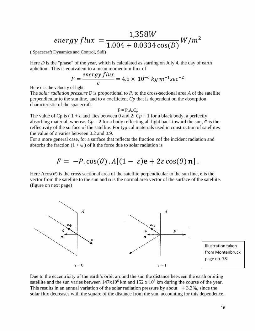
𝑒𝑛𝑒𝑟𝑔𝑦 𝑓𝑙𝑢𝑥 =1,358𝑊

1.004 + 0.0334 cos(𝐷)𝑊/𝑚2

( Spacecraft Dynamics and Control, Sidi)

Here D is the "phase" of the year, which is calculated as starting on July 4, the day of earth

aphelion . This is equivalent to a mean momentum flux of

𝑃 =𝑒𝑛𝑒𝑟𝑔𝑦 𝑓𝑙𝑢𝑥

𝑐= 4.5 × 10−6 𝑘𝑔 𝑚−1𝑠𝑒𝑐−2

Here c is the velocity of light.

The solar radiation pressure F is proportional to P, to the cross-sectional area A of the satellite

perpendicular to the sun line, and to a coefficient Cp that is dependent on the absorption

characteristic of the spacecraft. F = P.A.Cp

The value of Cp is ( 1 + 휀 and lies between 0 and 2; Cp = 1 for a black body, a perfectly

absorbing material, whereas Cp = 2 for a body reflecting all light back toward the sun, ∈ is the

reflectivity of the surface of the satellite. For typical materials used in construction of satellites

the value of 휀 varies between 0.2 and 0.9.

For a more general case, for a surface that reflects the fraction 휀of the incident radiation and

absorbs the fraction (1 + ∈ ) of it the force due to solar radiation is

𝐹 = −𝑃. cos(𝜃) . 𝐴[(1 − 휀)𝐞 + 2휀 cos(𝜃) 𝒏] .

Here Acos(𝜃) is the cross sectional area of the satellite perpendicular to the sun line, e is the

vector from the satellite to the sun and n is the normal area vector of the surface of the satellite.

(figure on next page)

Due to the eccentricity of the earth’s orbit around the sun the distance between the earth orbiting

satellite and the sun varies between 147x106 km and 152 x 106 km during the course of the year.

This results in an annual variation of the solar radiation pressure by about ∓ 3.3%, since the

solar flux decreases with the square of the distance from the sun. accounting for this dependence,

Illustration taken

from Montenbruck

page no. 78

17

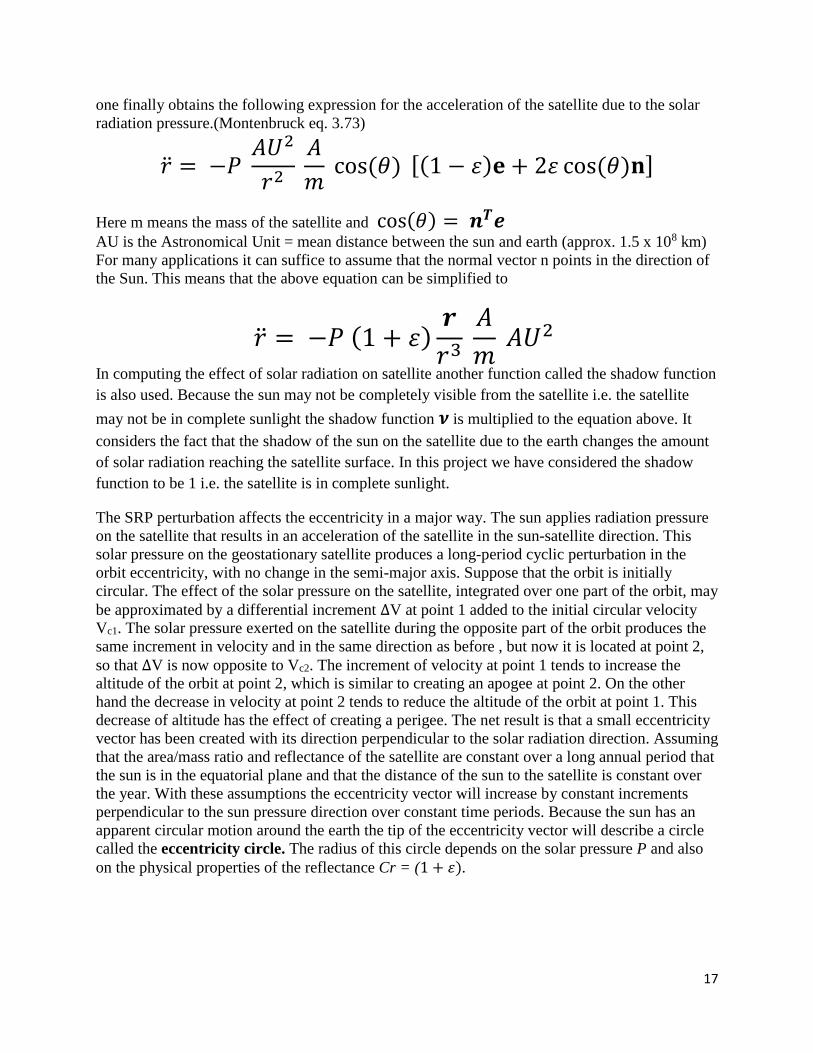
one finally obtains the following expression for the acceleration of the satellite due to the solar

radiation pressure.(Montenbruck eq. 3.73)

= −𝑃 𝐴𝑈2

𝑟2 𝐴

𝑚 cos(𝜃) [(1 − 휀)𝐞 + 2휀 cos(𝜃)𝐧]

Here m means the mass of the satellite and cos(𝜃) = 𝒏𝑻𝒆 AU is the Astronomical Unit = mean distance between the sun and earth (approx. 1.5 x 108 km)

For many applications it can suffice to assume that the normal vector n points in the direction of

the Sun. This means that the above equation can be simplified to

= −𝑃 (1 + 휀)𝒓

𝑟3 𝐴

𝑚 𝐴𝑈2

In computing the effect of solar radiation on satellite another function called the shadow function

is also used. Because the sun may not be completely visible from the satellite i.e. the satellite

may not be in complete sunlight the shadow function 𝝂 is multiplied to the equation above. It

considers the fact that the shadow of the sun on the satellite due to the earth changes the amount

of solar radiation reaching the satellite surface. In this project we have considered the shadow

function to be 1 i.e. the satellite is in complete sunlight.

The SRP perturbation affects the eccentricity in a major way. The sun applies radiation pressure

on the satellite that results in an acceleration of the satellite in the sun-satellite direction. This

solar pressure on the geostationary satellite produces a long-period cyclic perturbation in the

orbit eccentricity, with no change in the semi-major axis. Suppose that the orbit is initially

circular. The effect of the solar pressure on the satellite, integrated over one part of the orbit, may

be approximated by a differential increment ∆V at point 1 added to the initial circular velocity

Vc1. The solar pressure exerted on the satellite during the opposite part of the orbit produces the

same increment in velocity and in the same direction as before , but now it is located at point 2,

so that ∆V is now opposite to Vc2. The increment of velocity at point 1 tends to increase the

altitude of the orbit at point 2, which is similar to creating an apogee at point 2. On the other

hand the decrease in velocity at point 2 tends to reduce the altitude of the orbit at point 1. This

decrease of altitude has the effect of creating a perigee. The net result is that a small eccentricity

vector has been created with its direction perpendicular to the solar radiation direction. Assuming

that the area/mass ratio and reflectance of the satellite are constant over a long annual period that

the sun is in the equatorial plane and that the distance of the sun to the satellite is constant over

the year. With these assumptions the eccentricity vector will increase by constant increments

perpendicular to the sun pressure direction over constant time periods. Because the sun has an

apparent circular motion around the earth the tip of the eccentricity vector will describe a circle

called the eccentricity circle. The radius of this circle depends on the solar pressure P and also

on the physical properties of the reflectance Cr = (1 + 휀).

18

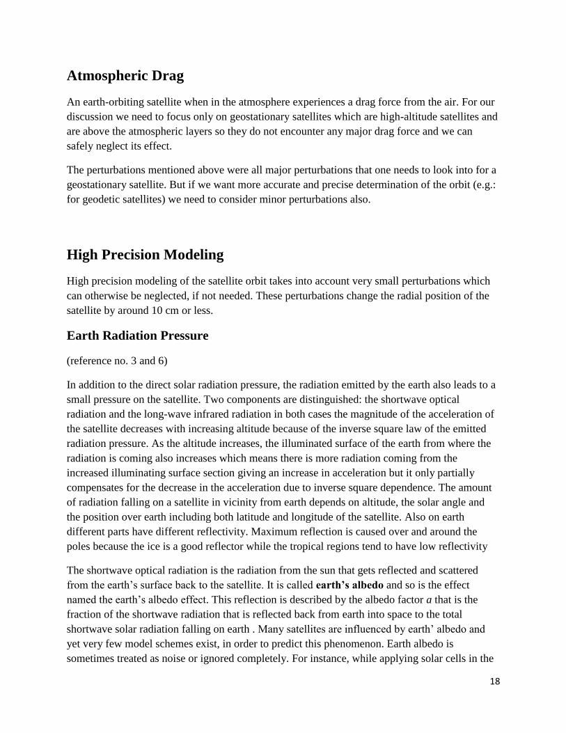
Atmospheric Drag

An earth-orbiting satellite when in the atmosphere experiences a drag force from the air. For our

discussion we need to focus only on geostationary satellites which are high-altitude satellites and

are above the atmospheric layers so they do not encounter any major drag force and we can

safely neglect its effect.

The perturbations mentioned above were all major perturbations that one needs to look into for a

geostationary satellite. But if we want more accurate and precise determination of the orbit (e.g.:

for geodetic satellites) we need to consider minor perturbations also.

High Precision Modeling

High precision modeling of the satellite orbit takes into account very small perturbations which

can otherwise be neglected, if not needed. These perturbations change the radial position of the

satellite by around 10 cm or less.

Earth Radiation Pressure

(reference no. 3 and 6)

In addition to the direct solar radiation pressure, the radiation emitted by the earth also leads to a

small pressure on the satellite. Two components are distinguished: the shortwave optical

radiation and the long-wave infrared radiation in both cases the magnitude of the acceleration of

the satellite decreases with increasing altitude because of the inverse square law of the emitted

radiation pressure. As the altitude increases, the illuminated surface of the earth from where the

radiation is coming also increases which means there is more radiation coming from the

increased illuminating surface section giving an increase in acceleration but it only partially

compensates for the decrease in the acceleration due to inverse square dependence. The amount

of radiation falling on a satellite in vicinity from earth depends on altitude, the solar angle and

the position over earth including both latitude and longitude of the satellite. Also on earth

different parts have different reflectivity. Maximum reflection is caused over and around the

poles because the ice is a good reflector while the tropical regions tend to have low reflectivity

The shortwave optical radiation is the radiation from the sun that gets reflected and scattered

from the earth’s surface back to the satellite. It is called earth’s albedo and so is the effect

named the earth’s albedo effect. This reflection is described by the albedo factor a that is the

fraction of the shortwave radiation that is reflected back from earth into space to the total

shortwave solar radiation falling on earth . Many satellites are influenced by earth’ albedo and

yet very few model schemes exist, in order to predict this phenomenon. Earth albedo is

sometimes treated as noise or ignored completely. For instance, while applying solar cells in the

19

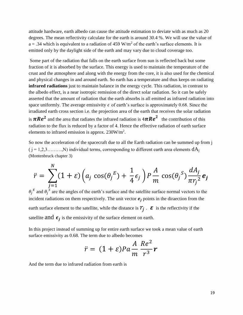
attitude hardware, earth albedo can cause the attitude estimation to deviate with as much as 20

degrees. The mean reflectivity calculate for the earth is around 30.4 %. We will use the value of

a = .34 which is equivalent to a radiation of 459 W/m2 of the earth’s surface elements. It is

emitted only by the daylight side of the earth and may vary due to cloud coverage too.

Some part of the radiation that falls on the earth surface from sun is reflected back but some

fraction of it is absorbed by the surface. This energy is used to maintain the temperature of the

crust and the atmosphere and along with the energy from the core, it is also used for the chemical

and physical changes in and around earth. So earth has a temperature and thus keeps on radiating

infrared radiations just to maintain balance in the energy cycle. This radiation, in contrast to

the albedo effect, is a near isotropic remission of the direct solar radiation. So it can be safely

asserted that the amount of radiation that the earth absorbs is all emitted as infrared radiation into

space uniformly. The average emissivity 𝜖 of earth’s surface is approximately 0.68. Since the

irradiated earth cross section i.e. the projection area of the earth that receives the solar radiation

is 𝝅𝑹𝒆𝟐 and the area that radiates the infrared radiation is 4𝝅𝑹𝒆𝟐 the contribution of this

radiation to the flux is reduced by a factor of 4. Hence the effective radiation of earth surface

elements to infrared emission is approx. 230W/m2.

So now the acceleration of the spacecraft due to all the Earth radiation can be summed up from j

( j = 1,2,3………,N) individual terms, corresponding to different earth area elements dAj

(Montenbruck chapter 3)

= ∑(1 + 휀)

𝑁

𝑗=1

(𝑎𝑗 cos(𝜃𝑗𝐸) +

1

4𝜖𝑗 ) 𝑃

𝐴

𝑚 cos(𝜃𝑗

𝑆)𝑑𝐴𝑗

𝜋𝑟𝑗2

𝒆𝒋

𝜃𝑗𝐸

and 𝜃𝑗𝑆 are the angles of the earth’s surface and the satellite surface normal vectors to the

incident radiations on them respectively. The unit vector 𝒆𝒋 points in the diraection from the

earth surface element to the satellite, while the distance is 𝑟𝑗 . 𝜺 is the reflectivity if the

satellite and 𝝐𝒋 is the emissivity of the surface element on earth.

In this project instead of summing up for entire earth surface we took a mean value of earth

surface emissivity as 0.68. The term due to albedo becomes

= (1 + 휀)𝑃𝑎𝐴

𝑚 𝑅𝑒2

𝑟3𝒓

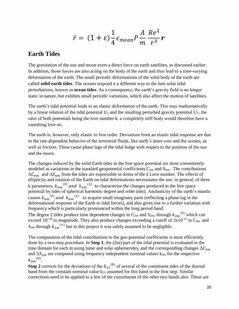
And the term due to infrared radiation from earth is

20

= (1 + 휀)1

4𝜖𝑚𝑒𝑎𝑛𝑃

𝐴

𝑚 𝑅𝑒2

𝑟3𝒓

Earth Tides

The gravitation of the sun and moon exert a direct force on earth satellites, as discussed earlier.

In addition, those forces are also acting on the body of the earth and thus lead to a time-varying

deformation of the earth. The small periodic deformations of the solid body of the earth are

called solid earth tides. The oceans respond n a different way to the luni-solar tidal

perturbations, known as ocean tides. As a consequence, the earth’s gravity field is no longer

static in nature, but exhibits small periodic variations, which also affect the motion of satellites.

The earth’s tidal potential leads to an elastic deformation of the earth. This may mathematically

by a linear relation of the tidal potential U2 and the resulting perturbed gravity potential UT, the

ratio of both potentials being the love number k. a completely stiff body would therefore have a

vanishing love no.

The earth is, however, only elastic to first order. Deviations from an elastic tidal response are due

to the rate-dependent behavior of the terrestrial fluids, like earth’s inner core and the oceans, as

well as friction. These cause phase lags of the tidal bulge with respect to the position of the sun

and the moon.

The changes induced by the solid Earth tides in the free space potential are most conveniently

modeled as variations in the standard geopotential coefficients Cnm and Snm . The contributions

Δ𝐶𝑛𝑚 and Δ𝑆𝑛𝑚 from the tides are expressible in terms of the k Love number. The effects of

ellipticity and rotation of the Earth on tidal deformations necessitates the use, in general, of three

k parameters, 𝑘𝑛𝑚(0) 𝑎𝑛𝑑 𝑘𝑛𝑚

(±) to characterize the changes produced in the free space

potential by tides of spherical harmonic degree and order (nm). Anelasticity of the earth’s mantle

causes 𝑘𝑛𝑚(0) 𝑎𝑛𝑑 𝑘𝑛𝑚

(±) to acquire small imaginary parts (reflecting a phase lag in the

deformational response of the Earth to tidal forces), and also gives rise to a further variation with

frequency which is particularly pronounced within the long period band.

The degree 2 tides produce time dependent changes in C2m and S2m, through 𝑘2𝑚(0)

which can

exceed 10−8 in magnitude. They also produce changes exceeding a cutoff of 3x10-12 in C4m and

S4m through 𝑘2𝑚(+)

but in this project it was safely assumed to be negligible.

The computation of the tidal contributions to the geo-potential coefficients is most efficiently

done by a two-step procedure. In Step 1, the (2m) part of the tidal potential is evaluated in the

time domain for each m using lunar and solar ephemerides, and the corresponding changes Δ𝐶2𝑚

and Δ𝑆2𝑚 are computed using frequency independent nominal values k2m for the respective

𝑘2𝑚(0).

Step 2 corrects for the deviations of the 𝑘21(0)

of several of the constituent tides of the diurnal

band from the constant nominal value k21 assumed for this band in the first step. Similar

corrections need to be applied to a few of the constituents of the other two bands also. These are

21

frequency dependent corrections and are of the order of 10-12 and below range and this report

neglects them too but for further accuracy they can be considered too (refer Doodson McCarthy).

With frequency-independent values knm (Step 1), changes induced by the (nm) part of the tide

generating potential in the normalized geo-potential coefficients having the same (nm) are given

in the time domain by ( chapter 6, McCarthy Doodson, IERS Technical Note 21)

∆𝑛𝑚 + 𝑖∆𝑛𝑚 = 𝑘𝑛𝑚

2𝑛 + 1 ∑

𝐺𝑀𝑗

𝐺𝑀(

𝑅𝑒

𝑟𝑗)

𝑛+1

𝑛𝑚(𝑠𝑖𝑛 ∅𝑗)𝑒−𝑖𝑚𝜆𝑗

3

𝑗=2

(with Sn0 = 0), where

knm = nominal degree Love number for degree n and order m,

Re = equatorial radius of the Earth,

GM = gravitational parameter for the Earth,

GMj = gravitational parameter for the Moon (j = 2) and Sun (j = 3),

rj = distance from geocenter to Moon or Sun,

∅𝑗 = body fixed geocentric latitude of Moon or Sun,

𝜆𝑗 = body fixed east longitude (from Greenwich) of Moon or Sun,

and 𝑛𝑚is the normalized associated Legendre function related to the classical (unnormalized)

one by 𝑛𝑚 = 𝑁𝑛𝑚𝑃𝑛𝑚 i.e.

𝑃𝑛 = √( 2 − 𝛿0𝑚)(2𝑛 + 1)(𝑛 − 𝑚)!

(𝑛 + 𝑚)! 𝑃𝑛𝑚

𝐶𝑛𝑚

𝑆𝑛𝑚 = √

( 2 − 𝛿0𝑚)(2𝑛 + 1)(𝑛 − 𝑚)!

(𝑛 + 𝑚)!

𝐶𝑛

𝑆𝑛

These values of the changes in geo-potential coefficients Is converted to unnormalized form and

then added to the coefficients used to evaluate the geo-potential perturbations (earth’s

oblateness). The values of k20 and k21 and k22 used are 0.29525, 0.29470, 0.29801

respectively.(McCarthy Doodson chapter 6)

Ocean Tides have a more dynamic and periodic effect with amplitudes one order of magnitude

less than the solid tides, so we did not consider these as perturbations but their effects can be

counted as noise.

CODE

% degree 2 love numbers for solid tides

k20 = 0.29525;

k21 = 0:29470;

k22 = 0.29801;

22

% multiplication factor of normalized and unnormalizd geopotential coeff

N20 = 2.236054;

N21 = 0.64363756;

N22 = 0.6443;

%solid tides

slat2 = atan2((Z3-Z1),(norm(X3-X1,Y3-Y1)));

% latitude of the sun

mlat2 = atan2((Z4-Z1),(norm(X4-X1,Y4-Y1)));

% latitude of the moon

ecefs= [ cos(hh) sin(hh) 0 ; -sin(hh) cos(hh) 0 ; 0 0 1]*[X3-X1 Y3-Y1 Z3-Z1]';

slong2=atan2(ecefs(2),ecefs(1)); % longitude of sun

ecefm= [ cos(hh) sin(hh) 0 ; -sin(hh) cos(hh) 0 ; 0 0 1]*[X4-X1 Y4-Y1 Z4-Z1]';

mlong2=atan2(ecefm(2),ecefm(1)); %longitude of moon

LEGENDRE POLYNOMIALS AS FUNCTION OF SUN AND MOON LATITUDE

Ps20 = (3*(sin(slat2))^2 - 1)/2;

Ps21 = 3*sin(slat2)*cos(slat2);

Ps22 = 3*(cos(slat2))^2;

Pm20 = (3*(sin(mlat2))^2 - 1)/2;

Pm21 = 3*sin(mlat2)*cos(mlat2);

Pm22 = 3*(cos(mlat2))^2;

%l = 2 , m=0

q20 = (G*m3/R13)*N20*Ps20 + (G*m4/R14)*N20*Pm20;

u20 = 0;

% normalized geopotential coefficients

delta_nC20 = (k20/5)*(Re^3/(G*m1))*q20;

delta_nS20 = (k20/5)*(Re^3/(G*m1))*u20;

% l=2, m=1;

q21 = (G*m3/R13^3)*Ps21*cos(slong2) + (G*m4/R14^3)*Pm21*cos(mlong2);

u21 = (G*m3/R13^3)*Ps21*sin(slong2) + (G*m4/R14^3)*Pm21*sin(mlong2);

%

delta_C21 = (k21/5)*(Re^3/G*m1)*q21;

delta_S21 = (k21/5)*(Re^3/G*m1)*u21;

% l= 2, m=2;

23

q22 = (G*m3/R13)*N22*Ps22*cos(2*slong2) + (G*m4/R14)*N22*Pm22*cos(2*mlong2);

u22 = (G*m3/R13)*N22*Ps22*sin(2*slong2) + (G*m4/R14)*N22*Pm22*sin(2*mlong2);

%

delta_nC22 = (k22/5)*(Re^3/G*m1)*q22;

delta_nS22 = (k22/5)*(Re^3/G*m1)*u22;

C20 = N20*(-484.165368e-6 + delta_nC20);

S20 = N20*(0 + delta_nS20);

C22 = N22*(2.439e-6 + delta_nC22);

S22 = N22*(-1.400266e-6 + delta_nS22);

Relativistic Effects

A rigorous treatment of the satellite’s motion should be formulated in accordance with the theory

of general relativity. While the special theory of relativity considers a flat four-dimensional

space-time, this is no longer true in the vicinity of the earth. Instead, the earth’s mass M with a

potential of U = GM / r and angular momentum lead to a curvature of the four-dimensional

space-time. Since the moon is much smaller than earth in size and mass and the sun is too far

away to have a considerable influence their relativistic effects on the satellite are neglected. The

calculation procedure is out of the scope of this project and thus we will only use a simplified

relation for the relativistic correction term in the Newtonian equation of motion under gravity.

The additional post-Newtonian space-time correction term of the acceleration is (ref. Montenbruck

chapter 3)

= − 𝐺𝑀

𝑟2 ((

4𝐺𝑚

𝑐2𝑟−

𝑣2

𝑐2 ) 𝒆𝒓 + 4

𝑣2

𝑐2(𝒆𝒓 . 𝒆𝒗 )𝒆𝒗 )

here 𝒆𝒓 and 𝒆𝒗 denote the unit position and unit velocity vector of the satellite in the e.c.i. frame.

For geostationary satellite the orbit is a near circle so 𝒆𝒓 and 𝒆𝒗 are perpendicular to each other

and the velocity square is 𝑣2 =𝐺𝑀

𝑟 . so the terms simplifies to

= − 𝐺𝑀

𝑟2 (3

𝑣2

𝑐2 ) 𝒆𝒓

This means the additional relativistic term is the Newtonian acceleration term multiplied by a

factor of 3𝑣2/𝑐2 which is roughly 3x10-8 for a typical satellite. Typically the effect of this

term on the radial position of the satellite is in centimeters.

24

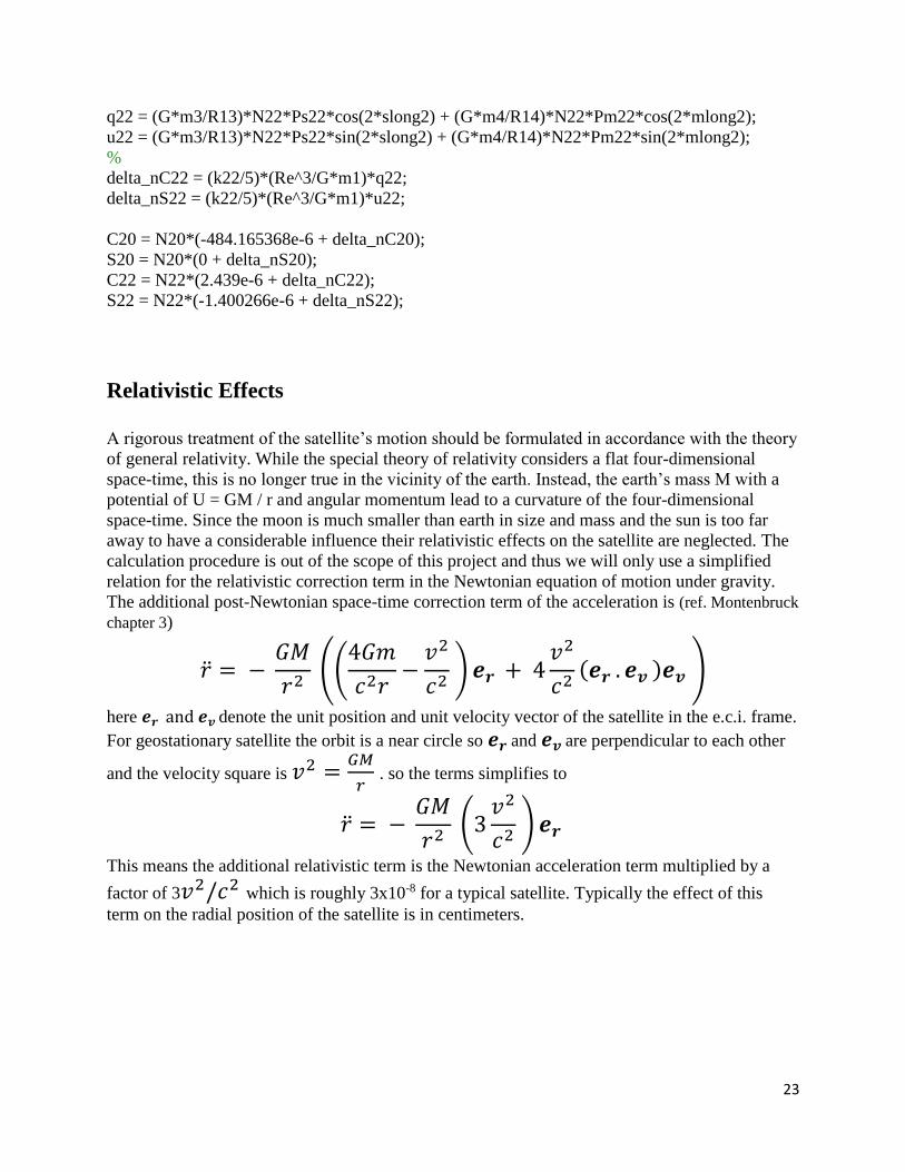
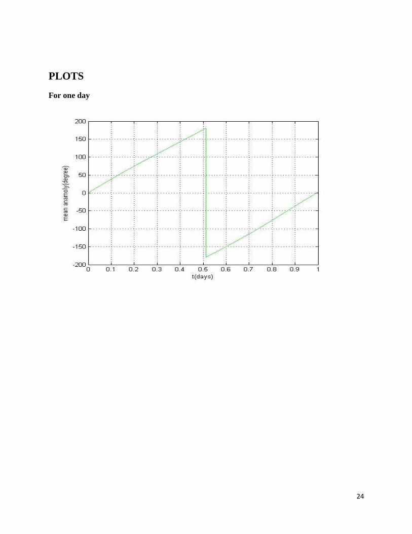
PLOTS

For one day

25

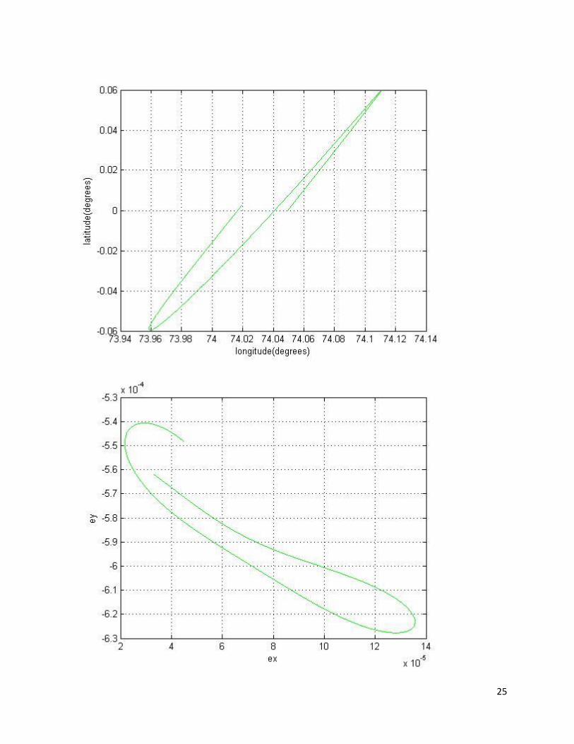
26

For one year

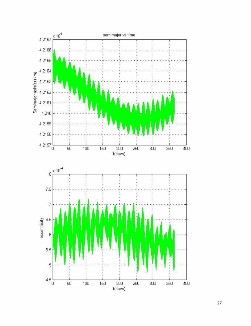
27

28

29

30

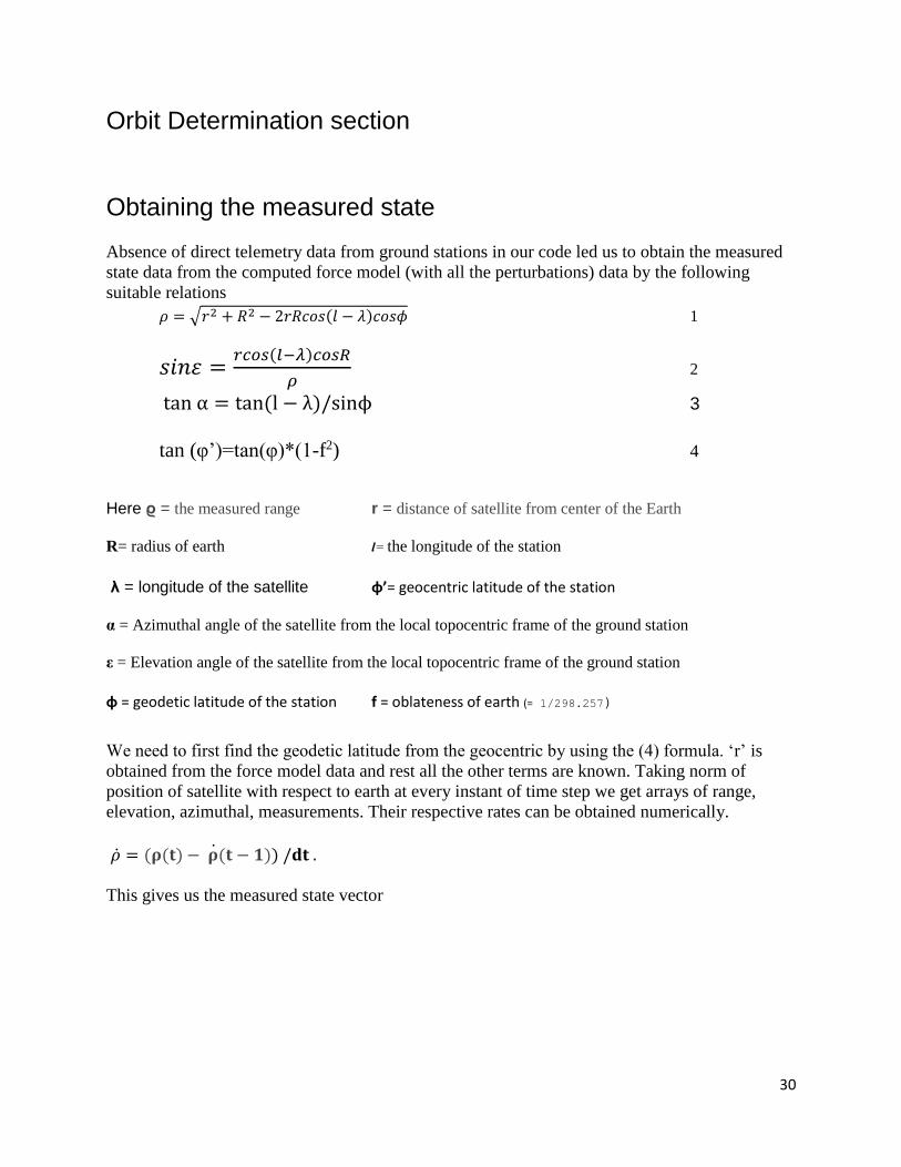
Orbit Determination section Obtaining the measured state Absence of direct telemetry data from ground stations in our code led us to obtain the measured

state data from the computed force model (with all the perturbations) data by the following

suitable relations

𝜌 = √𝑟2 + 𝑅2 − 2𝑟𝑅𝑐𝑜𝑠(𝑙 − 𝜆)𝑐𝑜𝑠𝜙 1

𝑠𝑖𝑛휀 =𝑟𝑐𝑜𝑠(𝑙−𝜆)𝑐𝑜𝑠𝑅

𝜌 2

tan α = tan(l − λ)/sinϕ 3

tan (φ’)=tan(φ)*(1-f2) 4

Here ϱ = the measured range r = distance of satellite from center of the Earth

R= radius of earth l= the longitude of the station

λ = longitude of the satellite φ’= geocentric latitude of the station α = Azimuthal angle of the satellite from the local topocentric frame of the ground station

ε = Elevation angle of the satellite from the local topocentric frame of the ground station

φ = geodetic latitude of the station f = oblateness of earth (= 1/298.257)

We need to first find the geodetic latitude from the geocentric by using the (4) formula. ‘r’ is

obtained from the force model data and rest all the other terms are known. Taking norm of

position of satellite with respect to earth at every instant of time step we get arrays of range,

elevation, azimuthal, measurements. Their respective rates can be obtained numerically.

= (𝛒(𝐭) − 𝛒(𝐭 − 𝟏)) /𝐝𝐭 .

This gives us the measured state vector

31

Calculation of the state vector from measurements of range, angular position and their rates

The fundamental vector triangle is formed by the topocentric position vector ϱ of

a satellite relative to a tracking station, the position vector R of the station relative

to the center of attraction C and the geocentric position vector r . The relationship among

these three vectors is given below. All the vectors are with respect to inertial coordinates

𝑟 = 𝑅 + 𝜌

𝑣 = = + 𝜌 + 𝜌

= unit vector along range vector

= angular velocity vector of earth

R=position vector of station

= range rate = unit range rate vector

V=velocity

Calculating Formulas and terms

Using the altitude H, latitude φ of the site and local sidereal time θ of the site, Re radius of

earth calculate its geocentric position vector R of the site.

𝑅 = [𝑅𝑒

√(1 − (2𝑓 − 𝑓2)𝑠𝑖𝑛2𝜙) + 𝐻] 𝑐𝑜𝑠𝜙(𝑐𝑜𝑠𝜃𝐼 + 𝑠𝑖𝑛𝜃𝐽)

+ [𝑅𝑒(1 − 𝑓)2

√(1 − (2𝑓 − 𝑓2)𝑠𝑖𝑛2𝜙) + 𝐻]𝑠𝑖𝑛𝜙

32

Since topocentric right ascension ( )/ declination ( ) are related to the azimuth (A) /elevation

(a) are related. They are calculated as follows

𝑠𝑖𝑛𝛿 = 𝑐𝑜𝑠𝜙𝑐𝑜𝑠𝐴𝑐𝑜𝑠𝑎 + 𝑠𝑖𝑛𝜙𝑠𝑖𝑛𝑎

For simplifying the equations for ( ) calculations we introduce the hour angle h,

ℎ = 𝜃 − 𝛼 h is the angular distance between the satellite and the local meridian (site longitude) . If h is

positive, the object is west of the meridian; if h is negative, the object is east of the meridian.

ℎ = 2𝜋 − 𝑐𝑜𝑠−1((𝑐𝑜𝑠𝜙𝑠𝑖𝑛𝑎 − 𝑠𝑖𝑛𝜙𝑐𝑜𝑠𝐴cos a)/cos𝛿) 0 < 𝐴 < 𝜋

𝑐𝑜𝑠−1 (𝑐𝑜𝑠𝜙𝑠𝑖𝑛𝑎−𝑠𝑖𝑛𝜙 𝑐𝑜𝑠𝐴 𝑐𝑜𝑠 𝑎

𝑐𝑜𝑠𝛿) 𝜋 < 𝐴 < 2𝜋

Therefore 𝛼 = 𝜃 − ℎ

The direction cosine unit vector is calculated as follows

= 𝑐𝑜𝑠𝛿(𝑐𝑜𝑠𝛼𝐼 + 𝑠𝑖𝑛𝛼𝐽) + 𝑠𝑖𝑛𝛿

Geocentric position vector r is finally calculted by 𝑟 = 𝑅 + 𝜌

And the inertial velocity ˙R of the site = ΩxR

Declination and right ascension angle rates and rate of change of unit range vector

=1

𝑐𝑜𝑠𝛿[−𝑐𝑜𝑠𝜙𝑠𝑖𝑛𝐴𝑐𝑜𝑠𝑎 + (𝑠𝑖𝑛𝜙𝑐𝑜𝑠𝑎 − 𝑐𝑜𝑠𝜙𝑐𝑜𝑠𝐴𝑠𝑖𝑛𝑎)]

= 𝜔𝐸 +𝑐𝑜𝑠𝐴𝑐𝑜𝑠𝑎−𝑠𝑖𝑛𝐴 𝑠𝑖𝑛𝑎+𝑠𝑖𝑛𝐴𝑐𝑜𝑠𝑎 𝑡𝑎𝑛𝛿

𝑐𝑜𝑠𝜙𝑠𝑖𝑛𝑎−𝑠𝑖𝑛𝜙𝑐𝑜𝑠𝐴𝑐𝑜𝑠𝑎

= (−𝑠𝑖𝑛𝛼 𝑐𝑜𝑠𝛿 − 𝑐𝑜𝑠𝛼 𝑠𝑖𝑛𝛿)𝐼 + (𝑐𝑜𝑠𝛼𝑐𝑜𝑠𝛿 − 𝑠𝑖𝑛𝛼𝑠𝑖𝑛𝛿)𝐽 + 𝑐𝑜𝑠𝛿

Finally the velocity of satellite in the ECI frame is 𝑉 = + + 𝜌

33

Batch Processing and Sequential Processing

Batch processing: We use it to find the initial position of the satellite which we have taken to be

known throughout the high fidelity force model .This is a method in which we have more

equations than the no of variables in measurements taken at different instants of time over a

period of time. We use it to find the initial position using least squares method at a particular

epoch at one of the measured instants.

Sequential Processing: The best known method of this type is Kalman filter –Classical and

Extended. The Extended is used in filtering in case of Non-linear equations. Here we use

extended since orbit determination model is non-linear .We first linearize the state space form

using the Taylor’s expansion. We first assume that we know the error covariance matrix initially

is known. The noise in the measurements is assumed to be of the white noise (Gaussian) form

that is with a mean of zero and a standard deviation of 1. The Kalman estimated value depends

whether there is more noise in the process or the measurements as it takes more weight of the

one with less covariance i.e. the one with less noise and it therefore it follows either process or

measurements. Unlike batch processing it gives estimated value at each measurement.

The Kalman Filtering

Theory: Linearizing the Non-Linear model of satellite Orbit for Kalman filtering

= 𝑓(𝑥, 𝑢𝑑 , 𝑡) + 𝑢(𝑡)

Z=h(x,t) +v(t)

f and h are known functions relating state to state derivatives

ud is a deterministic forcing function and u and v are white noises (whose initial estimates we assumed

to be known)

x(t)=x*(t) +∆𝑥(𝑡) x*(t)=approximate state as obtained from by force model 3

∆𝑥=addition to x* to get true (corrected) state x (it’s assumed

small )

𝑥 ∗ + ∆ = 𝑓(𝑥∗ + ∆𝑥, 𝑢𝑑 , 𝑡) + 𝑢(𝑡)

Z=ℎ(𝑥∗ + ∆𝑥, 𝑡) + 𝑣(𝑡)

Applying Taylor’s expansion to first order

∗ + ∆ ≈ 𝑓(𝑥∗, 𝑢𝑑 , 𝑡) + [𝜕𝑓

𝜕𝑥]𝑥=𝑥∗. ∆𝑥+u(t)

34

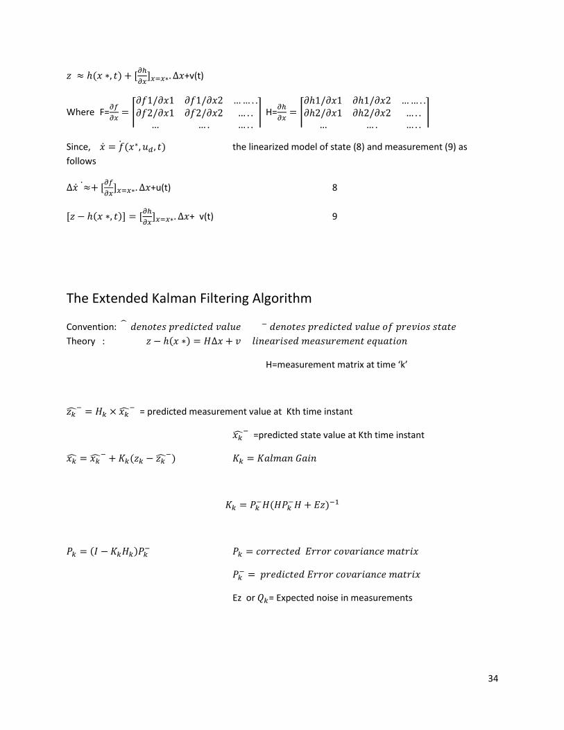
𝑧 ≈ ℎ(𝑥 ∗, 𝑡) + [𝜕ℎ

𝜕𝑥]𝑥=𝑥∗. ∆𝑥+v(t)

Where F=𝜕𝑓

𝜕𝑥= ⌈

𝜕𝑓1/𝜕𝑥1 𝜕𝑓1/𝜕𝑥2 … … . .𝜕𝑓2/𝜕𝑥1 𝜕𝑓2/𝜕𝑥2 … . .

… … . … . .⌉ H=

𝜕ℎ

𝜕𝑥= ⌈

𝜕ℎ1/𝜕𝑥1 𝜕ℎ1/𝜕𝑥2 … … . .𝜕ℎ2/𝜕𝑥1 𝜕ℎ2/𝜕𝑥2 … . .

… … . … . .⌉

Since, = 𝑓(𝑥∗, 𝑢𝑑 , 𝑡) the linearized model of state (8) and measurement (9) as

follows

∆ ≈ + [𝜕𝑓

𝜕𝑥]𝑥=𝑥∗. ∆𝑥+u(t) 8

[𝑧 − ℎ(𝑥 ∗, 𝑡)] = [𝜕ℎ

𝜕𝑥]𝑥=𝑥∗. ∆𝑥+ v(t) 9

The Extended Kalman Filtering Algorithm

Convention: 𝑑𝑒𝑛𝑜𝑡𝑒𝑠 𝑝𝑟𝑒𝑑𝑖𝑐𝑡𝑒𝑑 𝑣𝑎𝑙𝑢𝑒 − 𝑑𝑒𝑛𝑜𝑡𝑒𝑠 𝑝𝑟𝑒𝑑𝑖𝑐𝑡𝑒𝑑 𝑣𝑎𝑙𝑢𝑒 𝑜𝑓 𝑝𝑟𝑒𝑣𝑖𝑜𝑠 𝑠𝑡𝑎𝑡𝑒

Theory : 𝑧 − ℎ(𝑥 ∗) = 𝐻∆𝑥 + 𝑣 𝑙𝑖𝑛𝑒𝑎𝑟𝑖𝑠𝑒𝑑 𝑚𝑒𝑎𝑠𝑢𝑟𝑒𝑚𝑒𝑛𝑡 𝑒𝑞𝑢𝑎𝑡𝑖𝑜𝑛

H=measurement matrix at time ‘k’

𝑧− = 𝐻𝑘 × 𝑥

− = predicted measurement value at Kth time instant

𝑥− =predicted state value at Kth time instant

𝑥 = 𝑥− + 𝐾𝑘(𝑧𝑘 − 𝑧

−) 𝐾𝑘 = 𝐾𝑎𝑙𝑚𝑎𝑛 𝐺𝑎𝑖𝑛

𝐾𝑘 = 𝑃𝑘−𝐻(𝐻𝑃𝑘

−𝐻 + 𝐸𝑧)−1

𝑃𝑘 = (𝐼 − 𝐾𝑘𝐻𝑘)𝑃𝑘− 𝑃𝑘 = 𝑐𝑜𝑟𝑟𝑒𝑐𝑡𝑒𝑑 𝐸𝑟𝑟𝑜𝑟 𝑐𝑜𝑣𝑎𝑟𝑖𝑎𝑛𝑐𝑒 𝑚𝑎𝑡𝑟𝑖𝑥

𝑃𝑘− = 𝑝𝑟𝑒𝑑𝑖𝑐𝑡𝑒𝑑 𝐸𝑟𝑟𝑜𝑟 𝑐𝑜𝑣𝑎𝑟𝑖𝑎𝑛𝑐𝑒 𝑚𝑎𝑡𝑟𝑖𝑥

Ez or 𝑄𝑘= Expected noise in measurements

35

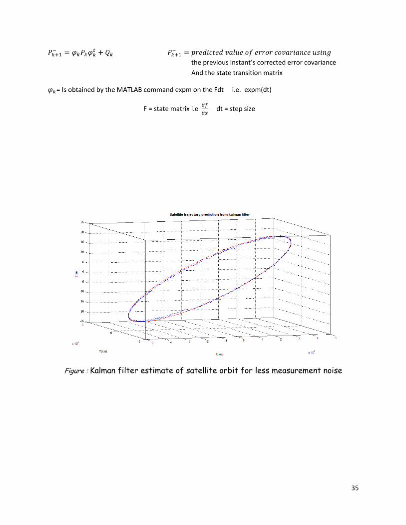
𝑃𝑘+1− = 𝜑𝑘𝑃𝑘𝜑𝑘

𝑡 + 𝑄𝑘 𝑃𝑘+1− = 𝑝𝑟𝑒𝑑𝑖𝑐𝑡𝑒𝑑 𝑣𝑎𝑙𝑢𝑒 𝑜𝑓 𝑒𝑟𝑟𝑜𝑟 𝑐𝑜𝑣𝑎𝑟𝑖𝑎𝑛𝑐𝑒 𝑢𝑠𝑖𝑛𝑔

the previous instant’s corrected error covariance

And the state transition matrix

𝜑𝑘= Is obtained by the MATLAB command expm on the Fdt i.e. expm(dt)

F = state matrix i.e 𝜕𝑓

𝜕𝑥 dt = step size

Figure : Kalman filter estimate of satellite orbit for less measurement noise

36

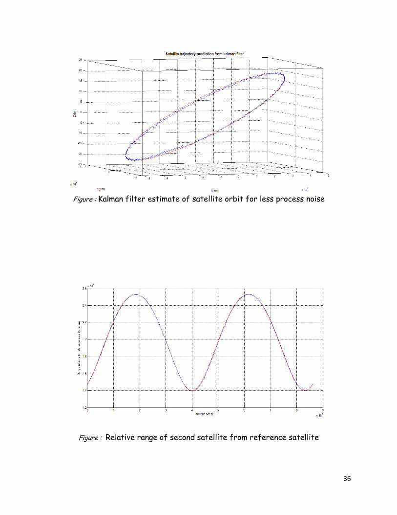
Figure : Kalman filter estimate of satellite orbit for less process noise

Figure : Relative range of second satellite from reference satellite

37

Figure : Estimated 7 satellite orbits

Figure : Relative range of 4 geosynchronous satellites from reference GEO satellite

38

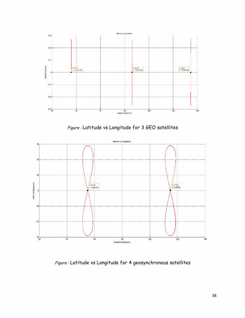
Figure : Latitude vs Longitude for 3 GEO satellites

Figure : Latitude vs Longitude for 4 geosynchronous satellites

39

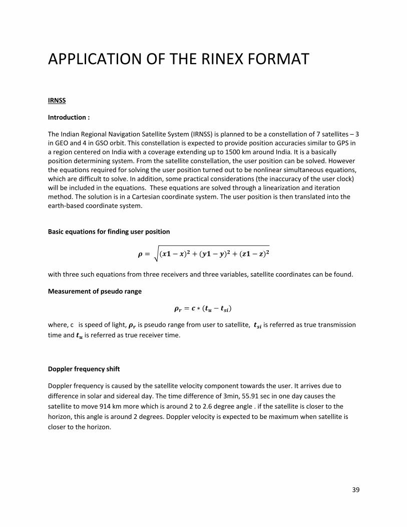
APPLICATION OF THE RINEX FORMAT

IRNSS

Introduction :

The Indian Regional Navigation Satellite System (IRNSS) is planned to be a constellation of 7 satellites – 3 in GEO and 4 in GSO orbit. This constellation is expected to provide position accuracies similar to GPS in a region centered on India with a coverage extending up to 1500 km around India. It is a basically position determining system. From the satellite constellation, the user position can be solved. However the equations required for solving the user position turned out to be nonlinear simultaneous equations, which are difficult to solve. In addition, some practical considerations (the inaccuracy of the user clock) will be included in the equations. These equations are solved through a linearization and iteration method. The solution is in a Cartesian coordinate system. The user position is then translated into the earth-based coordinate system.

Basic equations for finding user position

𝝆 = √(𝒙𝟏 − 𝒙)𝟐 + (𝒚𝟏 − 𝒚)𝟐 + (𝒛𝟏 − 𝒛)𝟐

with three such equations from three receivers and three variables, satellite coordinates can be found.

Measurement of pseudo range

𝝆𝒓 = 𝒄 ∗ (𝒕𝒖 − 𝒕𝒔𝒊)

where, c is speed of light, 𝝆𝒓 is pseudo range from user to satellite, 𝒕𝒔𝒊 is referred as true transmission

time and 𝒕𝒖 is referred as true receiver time.

Doppler frequency shift

Doppler frequency is caused by the satellite velocity component towards the user. It arrives due to

difference in solar and sidereal day. The time difference of 3min, 55.91 sec in one day causes the

satellite to move 914 km more which is around 2 to 2.6 degree angle . if the satellite is closer to the

horizon, this angle is around 2 degrees. Doppler velocity is expected to be maximum when satellite is

closer to the horizon.

40

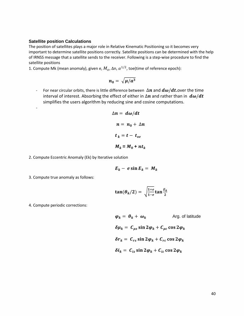
Satellite position Calculations The position of satellites plays a major role in Relative Kinematic Positioning so it becomes very important to determine satellite positions correctly. Satellite positions can be determined with the help of IRNSS message that a satellite sends to the receiver. Following is a step-wise procedure to find the satellite positions

1. Compute Mk (mean anomaly), given e, 𝑀𝑜, ∆n, 𝛼1/2, toe(time of reference epoch):

𝒏𝟎 = √𝝁/𝒂𝟑

- For near circular orbits, there is little difference between ∆𝒏 and 𝒅𝝎/𝒅𝒕.over the time interval of interest. Absorbing the effect of either in ∆𝒏 and rather than in 𝒅𝝎/𝒅𝒕 simplifies the users algorithm by reducing sine and cosine computations.

-

∆𝒏 = 𝒅𝝎/𝒅𝒕

𝒏 = 𝒏𝟎 + ∆𝒏

𝒕 𝒌 = 𝒕 − 𝒕𝒐𝒆

𝑴𝒌 = 𝑴𝟎 + 𝒏𝒕𝒌

2. Compute Eccentric Anomaly (Ek) by Iterative solution

𝑬𝒌 − 𝒆 𝐬𝐢𝐧 𝑬𝒌 = 𝑴𝒌

3. Compute true anomaly as follows:

𝐭𝐚𝐧(𝜽𝒌/𝟐) = √𝟏+𝒆

𝟏−𝒆𝐭𝐚𝐧

𝑬𝒌

𝟐

4. Compute periodic corrections:

𝝋𝒌 = 𝜽𝒌 + 𝝎𝒌 Arg. of latitude 𝜹𝝁𝒌 = 𝑪𝝁𝒔 𝐬𝐢𝐧 𝟐𝝋𝒌 + 𝑪𝝁𝒄 𝐜𝐨𝐬 𝟐𝝋𝒌

𝜹𝒓𝒌 = 𝑪𝒓𝒔 𝐬𝐢𝐧 𝟐𝝋𝒌 + 𝑪𝒓𝒄 𝐜𝐨𝐬 𝟐𝝋𝒌

𝜹𝒊𝒌 = 𝑪𝒊𝒔 𝐬𝐢𝐧 𝟐𝝋𝒌 + 𝑪𝒊𝒄 𝐜𝐨𝐬 𝟐𝝋𝒌

41

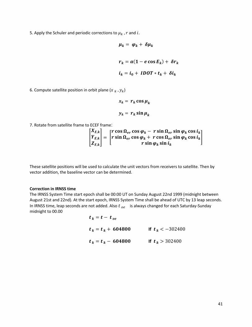
5. Apply the Schuler and periodic corrections to 𝜇𝑘 , 𝑟 and 𝑖.

𝝁𝒌 = 𝝋𝒌 + 𝜹𝝁𝒌

𝒓𝒌 = 𝒂(𝟏 − 𝒆 𝐜𝐨𝐬 𝑬𝒌) + 𝜹𝒓𝒌

𝒊𝒌 = 𝒊𝟎 + 𝑰𝑫𝑶𝑻 ∗ 𝒕𝒌 + 𝜹𝒊𝒌

6. Compute satellite position in orbit plane (𝑥 𝑘 , 𝑦𝑘) 𝒙𝒌 = 𝒓𝒌 𝐜𝐨𝐬 𝝁𝒌

𝒚𝒌 = 𝒓𝒌 𝐬𝐢𝐧 𝝁𝒌

7. Rotate from satellite frame to ECEF frame:

[

𝑿𝑬,𝒌

𝒀𝑬,𝒌

𝒁𝑬,𝒌

] = [

𝒓 𝐜𝐨𝐬 𝛀𝒆𝒓 𝐜𝐨𝐬 𝝋𝒌 − 𝒓 𝐬𝐢𝐧 𝛀𝒆𝒓 𝐬𝐢𝐧 𝝋𝒌 𝐜𝐨𝐬 𝒊𝒌

𝒓 𝐬𝐢𝐧 𝛀𝒆𝒓 𝐜𝐨𝐬 𝝋𝒌 + 𝒓 𝐜𝐨𝐬 𝛀𝒆𝒓 𝐬𝐢𝐧 𝝋𝒌 𝐜𝐨𝐬 𝒊𝒌

𝒓 𝐬𝐢𝐧 𝝋𝒌 𝐬𝐢𝐧 𝒊𝒌

]

These satellite positions will be used to calculate the unit vectors from receivers to satellite. Then by vector addition, the baseline vector can be determined. Correction in IRNSS time The IRNSS System Time start epoch shall be 00:00 UT on Sunday August 22nd 1999 (midnight between August 21st and 22nd). At the start epoch, IRNSS System Time shall be ahead of UTC by 13 leap seconds.

In IRNSS time, leap seconds are not added. Also 𝑡 𝑜𝑒 is always changed for each Saturday-Sunday midnight to 00.00

𝒕 𝒌 = 𝒕 − 𝒕 𝒐𝒆 𝒕 𝒌 = 𝒕 𝒌 + 𝟔𝟎𝟒𝟖𝟎𝟎 If 𝒕 𝒌 < −302400 𝒕 𝒌 = 𝒕 𝒌 − 𝟔𝟎𝟒𝟖𝟎𝟎 If 𝒕 𝒌 > 302400

42

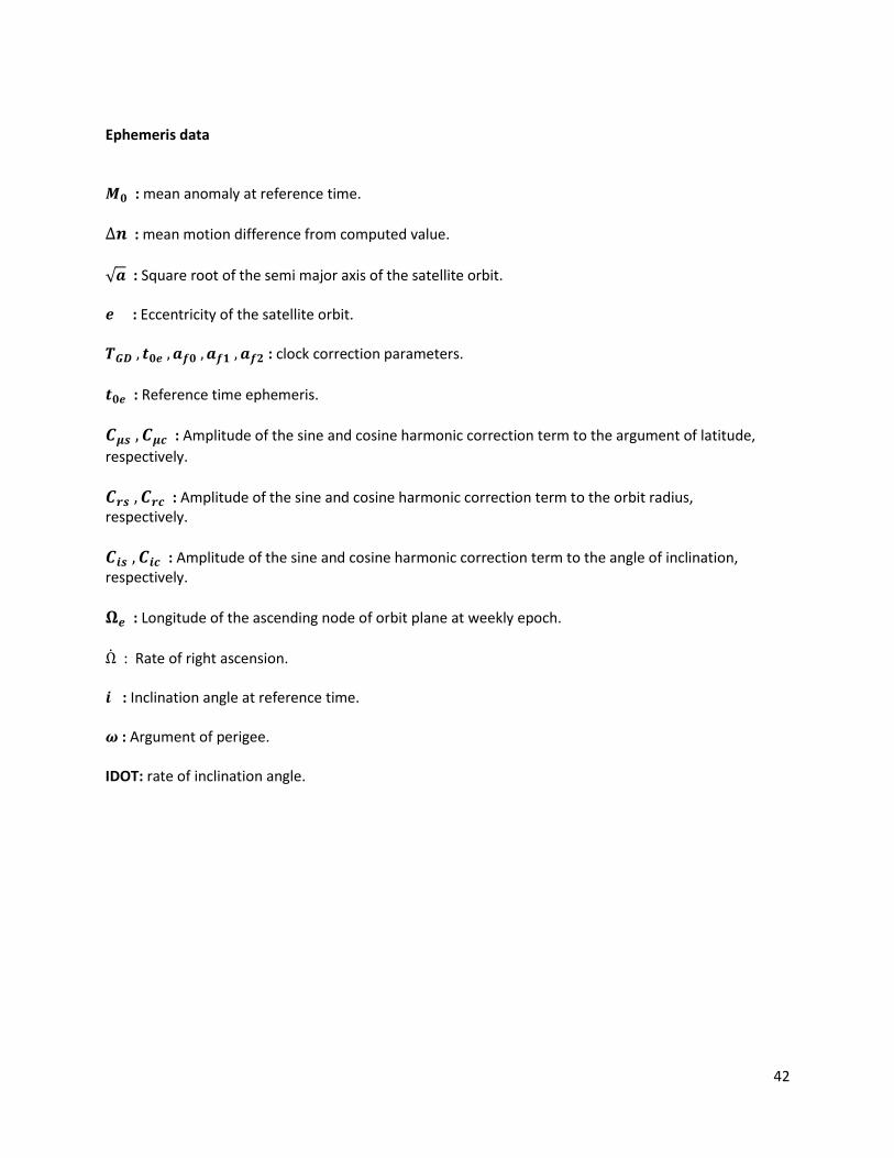
Ephemeris data 𝑴𝟎 : mean anomaly at reference time.

∆𝒏 : mean motion difference from computed value.

√𝒂 : Square root of the semi major axis of the satellite orbit. 𝒆 : Eccentricity of the satellite orbit. 𝑻𝑮𝑫 , 𝒕𝟎𝒆 , 𝒂𝒇𝟎 , 𝒂𝒇𝟏 , 𝒂𝒇𝟐 : clock correction parameters.

𝒕𝟎𝒆 : Reference time ephemeris.

𝑪𝝁𝒔 , 𝑪𝝁𝒄 : Amplitude of the sine and cosine harmonic correction term to the argument of latitude,

respectively.

𝑪𝒓𝒔 , 𝑪𝒓𝒄 : Amplitude of the sine and cosine harmonic correction term to the orbit radius, respectively.

𝑪𝒊𝒔 , 𝑪𝒊𝒄 : Amplitude of the sine and cosine harmonic correction term to the angle of inclination, respectively.

𝛀𝒆 : Longitude of the ascending node of orbit plane at weekly epoch.

Ω : Rate of right ascension. 𝒊 : Inclination angle at reference time. 𝝎 : Argument of perigee. IDOT: rate of inclination angle.

43

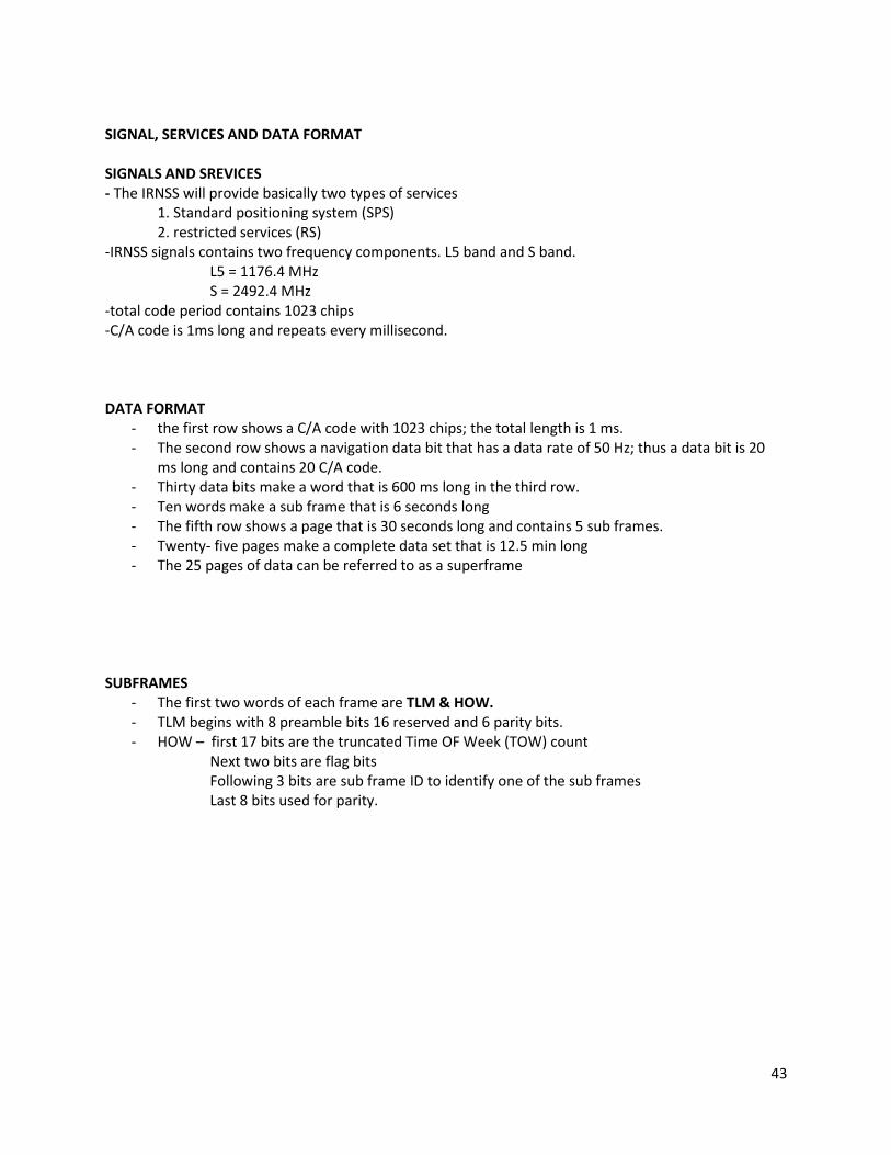
SIGNAL, SERVICES AND DATA FORMAT SIGNALS AND SREVICES - The IRNSS will provide basically two types of services 1. Standard positioning system (SPS) 2. restricted services (RS) -IRNSS signals contains two frequency components. L5 band and S band. L5 = 1176.4 MHz S = 2492.4 MHz -total code period contains 1023 chips -C/A code is 1ms long and repeats every millisecond. DATA FORMAT

- the first row shows a C/A code with 1023 chips; the total length is 1 ms. - The second row shows a navigation data bit that has a data rate of 50 Hz; thus a data bit is 20

ms long and contains 20 C/A code. - Thirty data bits make a word that is 600 ms long in the third row. - Ten words make a sub frame that is 6 seconds long - The fifth row shows a page that is 30 seconds long and contains 5 sub frames. - Twenty- five pages make a complete data set that is 12.5 min long - The 25 pages of data can be referred to as a superframe

SUBFRAMES

- The first two words of each frame are TLM & HOW. - TLM begins with 8 preamble bits 16 reserved and 6 parity bits. - HOW – first 17 bits are the truncated Time OF Week (TOW) count

Next two bits are flag bits Following 3 bits are sub frame ID to identify one of the sub frames Last 8 bits used for parity.

44

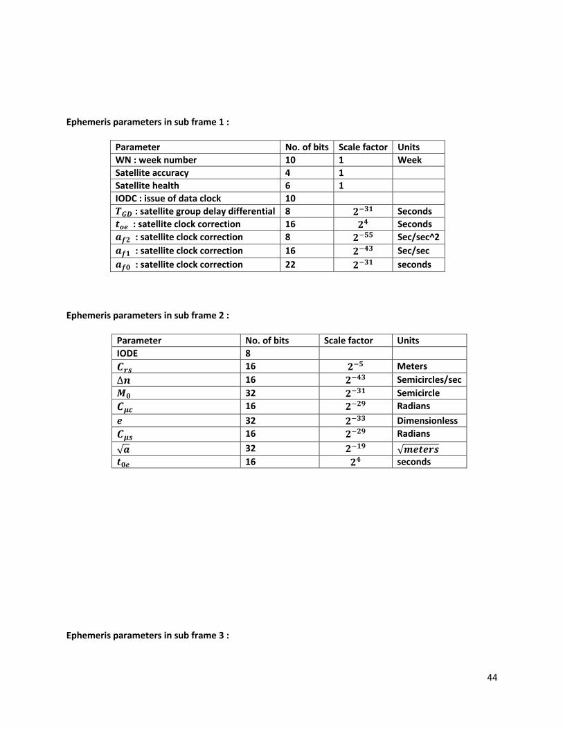
Ephemeris parameters in sub frame 1 :

Parameter No. of bits Scale factor Units

WN : week number 10 1 Week

Satellite accuracy 4 1

Satellite health 6 1

IODC : issue of data clock 10

𝑻𝑮𝑫 : satellite group delay differential 8 𝟐−𝟑𝟏 Seconds

𝒕𝒐𝒆 : satellite clock correction 16 𝟐𝟒 Seconds

𝒂𝒇𝟐 : satellite clock correction 8 𝟐−𝟓𝟓 Sec/sec^2

𝒂𝒇𝟏 : satellite clock correction 16 𝟐−𝟒𝟑 Sec/sec

𝒂𝒇𝟎 : satellite clock correction 22 𝟐−𝟑𝟏 seconds

Ephemeris parameters in sub frame 2 :

Parameter No. of bits Scale factor Units

IODE 8

𝑪𝒓𝒔 16 𝟐−𝟓 Meters

∆𝒏 16 𝟐−𝟒𝟑 Semicircles/sec

𝑴𝟎 32 𝟐−𝟑𝟏 Semicircle

𝑪𝝁𝒄 16 𝟐−𝟐𝟗 Radians

𝒆 32 𝟐−𝟑𝟑 Dimensionless

𝑪𝝁𝒔 16 𝟐−𝟐𝟗 Radians

√𝒂 32 𝟐−𝟏𝟗 √𝒎𝒆𝒕𝒆𝒓𝒔 𝒕𝟎𝒆 16 𝟐𝟒 seconds

Ephemeris parameters in sub frame 3 :

45

Parameters No. of bits Scale factor Units

𝑪𝒊𝒄 16 𝟐−𝟐𝟗 Radians

𝛀𝒆 32 𝟐−𝟑𝟏 Semicircles

𝑪𝒊𝒄 16 𝟐−𝟐𝟗 Radians

𝒊 32 𝟐−𝟑𝟏 Semicircles

𝑪𝒊𝒄 16 𝟐−𝟓 Meters

𝝎 32 𝟐𝟑𝟏 Semicircles

Ω 24 𝟐−𝟒𝟑 Semicircles/sec

IODE

IDOT 14 𝟐−𝟒𝟑 Semicircles/sec

Sub frame 4 :

- Pages 2, 3, 4, 5, 7, 8, 9 and 10 contains the almanac data for the satellite 25 through 32.these pages may be designed for the other functions. The satellite ID of that page defines the format and content.

- Page 17 contains special messages. - Page 18 contains ionospheric and universal coordinated time (UTC). - Page 25 contains antispoof flag, satellite configuration for 32 satellites, and satellite health for

satellites 25-32. - Pages 1, 6, 11, 12, 16, 19, 20, 21, 22, 23, and 24 are reversed. - Page 13, 14, and 15 are spares.

Sub frame 5 :

- Page 1-24 contain almanac data for the satellite 1 through 24. - Page 25 contains satellite health for the satellite 1 through 24, the almanac reference time, and

the almanac week number.

46

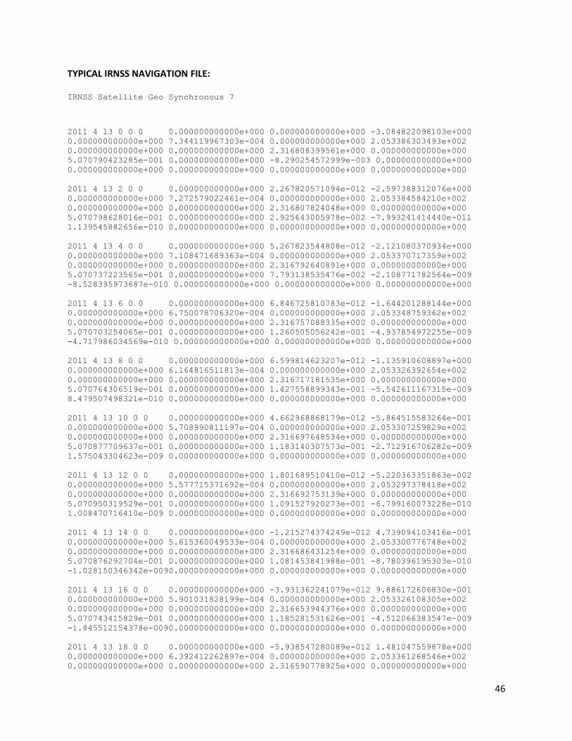
TYPICAL IRNSS NAVIGATION FILE: IRNSS Satellite Geo Synchronous 7

2011 4 13 0 0 0 0.000000000000e+000 0.000000000000e+000 -3.084822098103e+000

0.000000000000e+000 7.344119967303e-004 0.000000000000e+000 2.053386303493e+002

0.000000000000e+000 0.000000000000e+000 2.316808399561e+000 0.000000000000e+000

5.070790423285e-001 0.000000000000e+000 -8.290254572999e-003 0.000000000000e+000

0.000000000000e+000 0.000000000000e+000 0.000000000000e+000 0.000000000000e+000

2011 4 13 2 0 0 0.000000000000e+000 2.267820571094e-012 -2.597388312076e+000

0.000000000000e+000 7.272579022461e-004 0.000000000000e+000 2.053384584210e+002

0.000000000000e+000 0.000000000000e+000 2.316807824048e+000 0.000000000000e+000

5.070798628016e-001 0.000000000000e+000 2.925643005978e-002 -7.993241414440e-011

1.139545882656e-010 0.000000000000e+000 0.000000000000e+000 0.000000000000e+000

2011 4 13 4 0 0 0.000000000000e+000 5.267823544808e-012 -2.121080370934e+000

0.000000000000e+000 7.108471689363e-004 0.000000000000e+000 2.053370717359e+002

0.000000000000e+000 0.000000000000e+000 2.316792640891e+000 0.000000000000e+000

5.070737223565e-001 0.000000000000e+000 7.793138535476e-002 -2.108771782564e-009

-8.528395973687e-010 0.000000000000e+000 0.000000000000e+000 0.000000000000e+000

2011 4 13 6 0 0 0.000000000000e+000 6.846725810783e-012 -1.644201288144e+000

0.000000000000e+000 6.750078706320e-004 0.000000000000e+000 2.053348759362e+002

0.000000000000e+000 0.000000000000e+000 2.316757088335e+000 0.000000000000e+000

5.070703254065e-001 0.000000000000e+000 1.260505056242e-001 -4.937854972255e-009

-4.717986034569e-010 0.000000000000e+000 0.000000000000e+000 0.000000000000e+000

2011 4 13 8 0 0 0.000000000000e+000 6.599814623207e-012 -1.135910608897e+000

0.000000000000e+000 6.164816511813e-004 0.000000000000e+000 2.053326392654e+002

0.000000000000e+000 0.000000000000e+000 2.316717181535e+000 0.000000000000e+000

5.070764306519e-001 0.000000000000e+000 1.427558899343e-001 -5.542611167315e-009

8.479507498321e-010 0.000000000000e+000 0.000000000000e+000 0.000000000000e+000

2011 4 13 10 0 0 0.000000000000e+000 4.662968868179e-012 -5.864515583264e-001

0.000000000000e+000 5.708990811197e-004 0.000000000000e+000 2.053307259829e+002

0.000000000000e+000 0.000000000000e+000 2.316697648534e+000 0.000000000000e+000

5.070877709637e-001 0.000000000000e+000 1.183140307573e-001 -2.712916706282e-009

1.575043304623e-009 0.000000000000e+000 0.000000000000e+000 0.000000000000e+000

2011 4 13 12 0 0 0.000000000000e+000 1.801689510410e-012 -5.220363351863e-002

0.000000000000e+000 5.577715371692e-004 0.000000000000e+000 2.053297378418e+002

0.000000000000e+000 0.000000000000e+000 2.316692753139e+000 0.000000000000e+000

5.070950319529e-001 0.000000000000e+000 1.091527920273e-001 -6.799160073228e-010

1.008470716410e-009 0.000000000000e+000 0.000000000000e+000 0.000000000000e+000

2011 4 13 14 0 0 0.000000000000e+000 -1.215274374249e-012 4.739094103416e-001

0.000000000000e+000 5.615360049533e-004 0.000000000000e+000 2.053300776748e+002

0.000000000000e+000 0.000000000000e+000 2.316686431254e+000 0.000000000000e+000

5.070876292704e-001 0.000000000000e+000 1.081453841988e-001 -8.780396195303e-010

-1.028150346342e-0090.000000000000e+000 0.000000000000e+000 0.000000000000e+000

2011 4 13 16 0 0 0.000000000000e+000 -3.931362241079e-012 9.886172606830e-001

0.000000000000e+000 5.901031828199e-004 0.000000000000e+000 2.053326108305e+002

0.000000000000e+000 0.000000000000e+000 2.316653944376e+000 0.000000000000e+000

5.070743415829e-001 0.000000000000e+000 1.185281531626e-001 -4.512066383547e-009

-1.845512154378e-0090.000000000000e+000 0.000000000000e+000 0.000000000000e+000

2011 4 13 18 0 0 0.000000000000e+000 -5.938547280089e-012 1.481047559878e+000

0.000000000000e+000 6.392412262897e-004 0.000000000000e+000 2.053361268546e+002

0.000000000000e+000 0.000000000000e+000 2.316590778925e+000 0.000000000000e+000

47

5.070685160175e-001 0.000000000000e+000 1.511416183362e-001 -8.772979328183e-009

-8.091063035460e-0100.000000000000e+000 0.000000000000e+000 0.000000000000e+000

2011 4 13 20 0 0 0.000000000000e+000 -6.848366941609e-012 1.952860757550e+000

0.000000000000e+000 7.020780314763e-004 0.000000000000e+000 2.053387410142e+002

0.000000000000e+000 0.000000000000e+000 2.316523325165e+000 0.000000000000e+000

5.070793246071e-001 0.000000000000e+000 2.042970787536e-001 -9.368577695475e-009

1.501193002792e-009 0.000000000000e+000 0.000000000000e+000 0.000000000000e+000

2011 4 13 22 0 0 0.000000000000e+000 -6.180057924628e-012 2.416946443450e+000

0.000000000000e+000 7.479459555759e-004 0.000000000000e+000 2.053397456339e+002

0.000000000000e+000 0.000000000000e+000 2.316486589959e+000 0.000000000000e+000

5.071002824222e-001 0.000000000000e+000 2.651478848384e-001 -5.102111974329e-009

2.910807656868e-009 0.000000000000e+000 0.000000000000e+000 0.000000000000e+000

48

ACKNOWLEDGMENTS

We would like to express my gratitude to The Group Director of Controls division

Mr. P.M.Natarajan , A.K.Kulkarni & our supervisor, Mr. Vinod Kumar, Control

Dynamics and Simulation Group, ISRO Satellite Centre, whose expertise,

understanding and patience, added considerably to my experience. We appreciate his

vast knowledge and skill in many areas and even his ability to make a friendly

environment (e.g., vision, ethics, interaction with participants). His guidance and

supervision throughout the internship are the reason this project could give some

positive results. Finally, we would like to thank Prof. Hari B. Hablani, Aerospace

Engineering Department, IIT Mumbai for giving us an opportunity to work at ISRO

Satellite Centre and learn what could not have learnt otherwise, elsewhere.

49

REFERENCES

1. Spacecraft Dynamics and Control –A Practical Engineering Approach, Marcel J. Sidi

2. Curtis H., Orbital Mechanics[c] For Engineering Students (2005)(1st ed.)(en)(704s)

3. Satellite Orbits - Models, Methods and Applications, Montenbruck. E. Gill

4. Introduction to geostationary orbits, E Mattias Soop, European Space Operations Centre

5. Applied Orbit Perturbation and Maintenance , Chin-Chun “George” Chao

6. Spacecraft Attitude Determination and Control, Ed. By James R. Wertz

7. Fundamentals of Astrodynamics and Application, David A. Vallado

8. IERS Technical Note 21, IERS Conventions 1996, Denis D. McCarthy

9. Prospects for an improved Lense-Thirring Test with SLR and the GRACE Gravity

mission[paper], Glenn E. Peterson

10. Modeling Earth Albedo For Satellites In Earth Orbit[paper], Dan Bhanderi, Thomas Bak

11. Fundamentals of GPS receivers, a software approach, James Bao, Yen Tsui

12. Introduction to random signals and applied Kalman filtering by Robert Grover Brown

Y.C Hwang

13. IRNSS navigation message file Neetha