2013 A8 005 13A Final Report Prof Yip - pico.gov.hk

PUBLIC POLICY RESEARCH FUNDING SCHEME

公共政策研究資助計劃

Project Number : 項目編號：

2013.A8.005.13A

Project Title : 項目名稱：

A Study of the Movement of Type A and B Babies in Hong Kong 香港甲類嬰兒和乙類嬰兒的研究

Principal Investigator : 首席研究員：

Professor Paul S. F. YIP 葉兆輝教授

Institution/Think Tank : 院校／智庫：

The University of Hong Kong 香港大學

Project Duration (Month): 推行期 (月) ：

8

Funding (HK$) : 總金額 (HK$)：

308,706.00

This research report is uploaded onto the Central Policy Unit’s (CPU’s) website for public reference. The views expressed in this report are those of the Research Team of this project and do not represent the views of the CPU and/or the Assessment Panel. The CPU and/or the Assessment Panel do not guarantee the accuracy of the data included in this report.

Please observe the "Intellectual Property Rights & Use of Project Data” as stipulated in

the Guidance Notes of the Public Policy Research Funding Scheme. A suitable acknowledgement of the funding from the CPU should be included in any

publication/publicity arising from the work done on a research project funded in whole or in part by the CPU.

The English version shall prevail whenever there is any discrepancy between the

English and Chinese versions. 此研究報告已上載至中央政策組(中策組)網站，供公眾查閱。報告內所表達的意見純屬本

項目研究團隊的意見，並不代表中策組及／或評審委員會的意見。中策組及／或評審委員會不保

證報告所載的資料準確無誤。請遵守公共政策研究資助計劃申請須知內關於「知識產權及項目數據的使用」的規定。接受中策組全數或部分資助的研究項目如因研究工作須出版任何刊物／作任何宣傳，均

須在其中加入適當鳴謝，註明獲中策組資助。

中英文版本如有任何歧異，概以英文版本為準。

A STUDY OF THE MOVEMENT OF TYPE A AND B

BABIES IN HONG KONG

香港甲類嬰兒和乙類嬰兒的研究

Research Team:

Prof Paul Yip (Principal Investigator)Dr Eddy Lam

Dr Mehdi SoleymaniMr Siulun Chow

The University of Hong Kong

December 2014

CONTENTS CONTENTS

Contents

1 Executive Summary 6

2 Recommendations 7

3 Background 8

3.1 Social Issues associated with Returning Children . . . . . . . . . . . . . . . . . . . . . . 83.2 Classifications of Returning Children . . . . . . . . . . . . . . . . . . . . . . . . . . . . . 83.3 Aims of Study . . . . . . . . . . . . . . . . . . . . . . . . . . . . . . . . . . . . . . . . . . . 9

4 Data Management 9

4.1 Data Set 1: Movement Records of Type A and Type B Children . . . . . . . . . . . . . . 94.2 Data Set 2: Birth Information . . . . . . . . . . . . . . . . . . . . . . . . . . . . . . . . . . 11

5 Traveling Patterns 12

5.1 First Departure . . . . . . . . . . . . . . . . . . . . . . . . . . . . . . . . . . . . . . . . . . 125.2 First Arrival . . . . . . . . . . . . . . . . . . . . . . . . . . . . . . . . . . . . . . . . . . . . 13

6 Return Rates 14

6.1 Return Rates by Ages and Birth Cohorts . . . . . . . . . . . . . . . . . . . . . . . . . . . . 146.2 Return Rate by Mother’s Occupation . . . . . . . . . . . . . . . . . . . . . . . . . . . . . . 146.3 Return Rate by Father’s Occupation . . . . . . . . . . . . . . . . . . . . . . . . . . . . . . 166.4 Return rate by Mother’s Education Level . . . . . . . . . . . . . . . . . . . . . . . . . . . 176.5 Return rate by Father’s Education Level . . . . . . . . . . . . . . . . . . . . . . . . . . . . 176.6 Estimation of Return Rate for the Coming Years . . . . . . . . . . . . . . . . . . . . . . . 18

7 Cross-border Students 20

7.1 Estimation of Number of Cross-border Students . . . . . . . . . . . . . . . . . . . . . . . 20

8 Family Backgrounds 21

8.1 Occupations of the Parents of Type A and Type B Children . . . . . . . . . . . . . . . . . 218.2 Education of Parents of Type A and Type B Children . . . . . . . . . . . . . . . . . . . . . 22

Appendices 23

A Number of Type A and Type I children 24

B Parents’ Occupation 25

C Combination of Parents’ Occupations 26

D Parents’ Education 29

E Combination of Parents’ Education Levels 30

2

LIST OF TABLES LIST OF TABLES

F Age of Childbearing 33

G Age of Marriage 34

H Years between Marriage and Childbearing 34

I Hospital of Birth 36

J Discrete Markov Chain 36

References 38

List of Tables

1 Classification of types of children based on father’s residency status. . . . . . . . . . . . 82 Distribution of Type A and Type B children in each data year. . . . . . . . . . . . . . . . 103 Use of arrival and departure points. . . . . . . . . . . . . . . . . . . . . . . . . . . . . . . 104 Births of Type A and Type B children per year. . . . . . . . . . . . . . . . . . . . . . . . . 115 Statistics on the number of days between birth and first departure. . . . . . . . . . . . . 136 Percentage of first arrivals by cohort and year. . . . . . . . . . . . . . . . . . . . . . . . . 137 Cumulative return rate of Type A and Type B children at each age by birth cohort. . . . 148 Return rate by mother’s occupation per birth cohort at 2014. . . . . . . . . . . . . . . . . 169 Return rate by father’s occupation per birth cohort at 2013. . . . . . . . . . . . . . . . . . 1610 Return rate by mother’s education level per birth cohort at 2013. . . . . . . . . . . . . . 1711 Return rate by father’s education level per birth cohort at 2013. . . . . . . . . . . . . . . 1812 Estimation of cumulative return rate by the Markov chain. . . . . . . . . . . . . . . . . . 1813 Predictions on the number of cross-border students per age and birth cohort. . . . . . . 2114 Number of Type A and Type I children from 2006 to 2013. . . . . . . . . . . . . . . . . . . 2415 Occupations of Type A and Type B mothers per year (%). . . . . . . . . . . . . . . . . . . 2516 Occupations of Type A and Type B fathers per year (%). . . . . . . . . . . . . . . . . . . 2517 Occupation of Type A mothers per father’s occupation (%). . . . . . . . . . . . . . . . . 2818 Occupation of Type B mothers per father’s occupation (%). . . . . . . . . . . . . . . . . 2819 Comparison of combination of parents’ occupations per year. . . . . . . . . . . . . . . . 2920 Education level of Type A and Type B mothers per year (%). . . . . . . . . . . . . . . . . 2921 Education level of Type A and Type B fathers per year (%). . . . . . . . . . . . . . . . . . 3022 Education level of Type A mothers per father’s education level (marginal %). . . . . . . 3223 Education level of Type B mothers per father’s education level (marginal %). . . . . . . 3224 Comparison of combination of parents’ education levels per year. . . . . . . . . . . . . . 3225 Median childbearing age of Hong Kong females, Type A mothers, and Type B mothers. 3326 Median first marriage age of local couples, Type A parents, and Type B parents. . . . . . 3427 Differences of median year between childbearing and marriage. . . . . . . . . . . . . . . 3528 Types of hospital used to give birth (%). . . . . . . . . . . . . . . . . . . . . . . . . . . . . 36

3

LIST OF FIGURES LIST OF FIGURES

List of Figures

1 Distribution of Type A, Type B, and other children from 2006 to 2012. . . . . . . . . . . . 122 Cumulative return rate of Type A children of all ages by birth cohort. . . . . . . . . . . 153 Cumulative return rate of Type B children of all ages by birth cohort. . . . . . . . . . . . 154 Prediction of cumulative return rate. . . . . . . . . . . . . . . . . . . . . . . . . . . . . . . 195 Number of estimated cross-border students. . . . . . . . . . . . . . . . . . . . . . . . . . 206 Occupations of Type A and Type B mothers per year (%). . . . . . . . . . . . . . . . . . . 267 Occupations of Type A and Type B fathers per year (%). . . . . . . . . . . . . . . . . . . 278 Combination of parents’ occupation . . . . . . . . . . . . . . . . . . . . . . . . . . . . . . 299 Education level of parents of Type A and Type B children (%). . . . . . . . . . . . . . . . 3110 Combination of parents’ education level . . . . . . . . . . . . . . . . . . . . . . . . . . . . 3311 Median childbearing age of Hong Kong females, Type A mothers, and Type B mothers. 3312 Age differences within local couples (first marriage), Type A parents, and Type B parents. 3513 Differences of median year between childbearing and marriage . . . . . . . . . . . . . . 35

4

LIST OF FIGURES LIST OF FIGURES

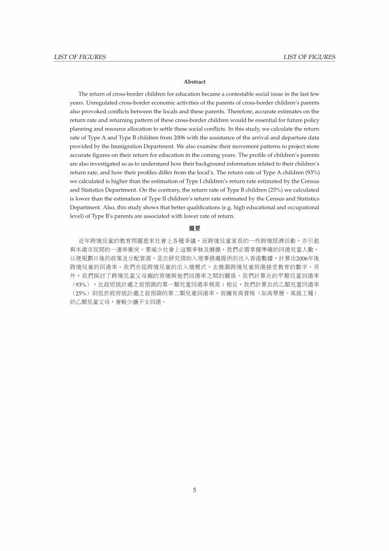
Abstract

The return of cross-border children for education became a contestable social issue in the last fewyears. Unregulated cross-border economic activities of the parents of cross-border children’s parentsalso provoked conflicts between the locals and these parents. Therefore, accurate estimates on thereturn rate and returning pattern of these cross-border children would be essential for future policyplanning and resource allocation to settle these social conflicts. In this study, we calculate the returnrate of Type A and Type B children from 2006 with the assistance of the arrival and departure dataprovided by the Immigration Department. We also examine their movement patterns to project moreaccurate figures on their return for education in the coming years. The profile of children’s parentsare also investigated so as to understand how their background information related to their children’sreturn rate, and how their profiles differ from the local’s. The return rate of Type A children (93%)we calculated is higher than the estimation of Type I children’s return rate estimated by the Censusand Statistics Department. On the contrary, the return rate of Type B children (25%) we calculatedis lower than the estimation of Type II children’s return rate estimated by the Census and StatisticsDepartment. Also, this study shows that better qualifications (e.g. high educational and occupationallevel) of Type B’s parents are associated with lower rate of return.

撮撮撮要要要

近年跨境兒童的教育問題惹來社會上各種爭議，而跨境兒童家長的一些跨境經濟活動，亦引起

與本港市民間的一連串衝突。要減少社會上這類爭執及磨擦，我們必需掌握準確的回港兒童人數，

以便規劃日後的政策及分配資源。是次研究借助入境事務處提供的出入香港數據，計算出2006年後跨境兒童的回港率。我們亦從跨境兒童的出入境模式，去推測跨境兒童到港接受教育的數字。另

外，我們探討了跨境兒童父母親的背境與他們回港率之間的關係。我們計算出的甲類兒童回港率

（93%），比政府統計處之前預測的第一類兒童回港率稍高；相反，我們計算出的乙類兒童回港率（25%）則低於政府統計處之前預測的第二類兒童回港率。而擁有高資格（如高學歷、高級工種）的乙類兒童父母，會較少讓子女回港。

5

1 EXECUTIVE SUMMARY

1 Executive Summary

Definition of Type A and Type B children: On the basis of the dataset provided by the ImmigrationDepartment, Type A children are those born in Hong Kong to Mainland parents and whose fathersare Hong Kong residents and Type B children are those born in Hong Kong to Mainland parents andwhose fathers are not Hong Kong residents.

1. The movements of 252,730 Type A and B children born after July 2004 are recorded in the database.

2. On average, Type A children leave Hong Kong for the first time 50 days after their birth date andType B children after 23 days.

3. Following their first departure, most of the children have a short visit to Hong Kong before theyreach the age of 2.

4. Lo Wu is the busiest checking point for recording Type A children’s movements, and ShenzhenBay is the busiest checking point for recording Type B children’s movements.

5. More than 93% of Type A children will return to Hong Kong (more that 77% at the age of 3 orbefore) compared to the Census and Statistics Department’s estimation(the figures are directlyprovided by the C&SD per request): 92% of Type I children (84% at the age of 3 or before).

6. More than 25% of Type B children will return to Hong Kong (more than 21% at the age of 6 orbefore) compared to the Census and Statistics Department’s estimation(the figures are directlyprovided by the C&SD per request): 40% of Type II children (41% at the age of 6 or before).

7. An analysis of the data set shows that in 2013/14, there were:

(a) 2,933 3-year-old cross-border pupils,

(b) 2,618 4-year-old cross-border pupils,

(c) 2,335 5-year-old cross-border pupils, and

(d) 1,912 6-year-old cross-border pupils.

8. The parents of Type B children seems have better educational and occupational qualifications (inproportion), but the return rate of their children is much lower than that of Type A children.

9. The better qualifications of the parents of Type B children are related to the lower rate of return:The higher qualifications (education or occupation) of the parents of Type B children mean that itis less likely that they would let their children return to Hong Kong.

Acknowledgment: The research team is grateful to the support of Secretary of Security and theDirector of Immigration Department and his staff who provide the necessary data for the project. Theresearch team has also been benefited from the discussion with the Census and Statistics Departmentand the support from the Education Bureau.

6

2 RECOMMENDATIONS

2 Recommendations

1. In comparing to the preliminary estimates by C&SD on the return rates of Type I and II children,it was found that more (less) than expected Type A (B) children returning to Hong Kong. Theseestimates should be taken into account in the population projection of Hong Kong in later years.

2. Apparently, there is a gradual improvement of the education attainment level of parents of bothType A and Type B children. Nevertheless, amongst those, the return rate of the tertiary educatedones is relatively less than the others.

3. The relevant Bureau should examine the carrying capacity of various checkpoints especially inShenzhen Bay for the Type B children.

4. The number of cross-border children have been estimated and the provision of school placesshould be reexamined in view of the latest estimate.

5. Streamlining the movement process for cross-border school children should be considered toreduce the unpleasant daily long journey time especially for young school children.

6. The movement data of cross-border children captured by the Immigration department providesvery useful information about the population flow of Hong Kong population. The monitoringand surveillance exercise should be in place as a regular basis to assess changes of inflow andoutflow of the population. The monitoring system should be done on a regular basis to providerelevant information for any population policy formulation of Hong Kong.

7

3 BACKGROUND

3 Background

3.1 Social Issues associated with Returning Children

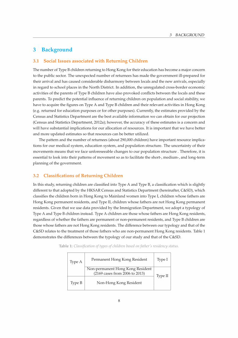
The number of Type B children returning to Hong Kong for their education has become a major concernto the public sector. The unexpected number of returnees has made the government ill-prepared fortheir arrival and has caused considerable disharmony between locals and the new arrivals, especiallyin regard to school places in the North District. In addition, the unregulated cross-border economicactivities of the parents of Type B children have also provoked conflicts between the locals and theseparents. To predict the potential influence of returning children on population and social stability, wehave to acquire the figures on Type A and Type B children and their relevant activities in Hong Kong(e.g. returned for education purposes or for other purposes). Currently, the estimates provided by theCensus and Statistics Department are the best available information we can obtain for our projection(Census and Statistics Department, 2012a); however, the accuracy of these estimates is a concern andwill have substantial implications for our allocation of resources. It is important that we have betterand more updated estimates so that resources can be better utilized.

The pattern and the number of returnees (about 290,000 children) have important resource implica-tions for our medical system, education system, and population structure. The uncertainty of theirmovements means that we face unforeseeable changes to our population structure . Therefore, it isessential to look into their patterns of movement so as to facilitate the short-, medium-, and long-termplanning of the government.

3.2 Classifications of Returning Children

In this study, returning children are classified into Type A and Type B, a classification which is slightlydifferent to that adopted by the HKSAR Census and Statistics Department (hereinafter, C&SD), whichclassifies the children born in Hong Kong to Mainland women into Type I, children whose fathers areHong Kong permanent residents, and Type II, children whose fathers are not Hong Kong permanentresidents. Given that we use data provided by the Immigration Department, we adopt a typology ofType A and Type B children instead. Type A children are those whose fathers are Hong Kong residents,regardless of whether the fathers are permanent or non-permanent residents, and Type B children arethose whose fathers are not Hong Kong residents. The difference between our typology and that of theC&SD relates to the treatment of those fathers who are non-permanent Hong Kong residents. Table 1demonstrates the differences between the typology of our study and that of the C&SD.

Table 1: Classification of types of children based on father’s residency status.

Type A Permanent Hong Kong Resident Type I

Non-permanent Hong Kong Resident

Type II(2169 cases from 2006 to 2013)

Non-Hong Kong ResidentType B

8

3.3 Aims of Study 4 DATA MANAGEMENT

3.3 Aims of Study

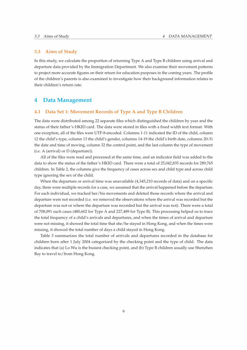
In this study, we calculate the proportion of returning Type A and Type B children using arrival anddeparture data provided by the Immigration Department. We also examine their movement patternsto project more accurate figures on their return for education purposes in the coming years. The profileof the children’s parents is also examined to investigate how their background information relates totheir children’s return rate.

4 Data Management

4.1 Data Set 1: Movement Records of Type A and Type B Children

The data were distributed among 22 separate files which distinguished the children by year and thestatus of their father’s HKID card. The data were stored in files with a fixed width text format. Withone exception, all of the files were UTF-8-encoded. Columns 1-11 indicated the ID of the child, column12 the child’s type, column 13 the child’s gender, columns 14-19 the child’s birth date, columns 20-31the date and time of moving, column 32 the control point, and the last column the type of movement(i.e. A (arrival) or D (departure)).

All of the files were read and processed at the same time, and an indicator field was added to thedata to show the status of the father’s HKID card. There were a total of 25,042,835 records for 289,765children. In Table 2, the columns give the frequency of cases across sex and child type and across childtype ignoring the sex of the child.

When the departure or arrival time was unavailable (4,345,210 records of data) and on a specificday, there were multiple records for a case, we assumed that the arrival happened before the departure.For each individual, we tracked her/his movements and deleted those records where the arrival anddeparture were not recorded (i.e. we removed the observations where the arrival was recorded but thedeparture was not or where the departure was recorded but the arrival was not). There were a totalof 708,091 such cases (480,602 for Type A and 227,489 for Type B). This processing helped us to tracethe total frequency of a child’s arrivals and departures, and when the times of arrival and departurewere not missing, it showed the total time that she/he stayed in Hong Kong, and when the times weremissing, it showed the total number of days a child stayed in Hong Kong.

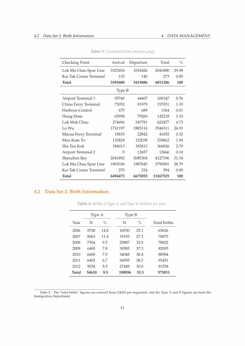
Table 3 summarizes the total number of arrivals and departures recorded in the database forchildren born after 1 July 2004 categorized by the checking point and the type of child. The dataindicates that (a) Lo Wu is the busiest checking point, and (b) Type B children usually use ShenzhenBay to travel to/from Hong Kong.

9

4.1 Data Set 1: Movement Records of Type A and Type B Children 4 DATA MANAGEMENT

Table 2: Distribution of Type A and Type B children in each data year.

Year Sex

of F M Total

Birth A B A B A B All

1997 814 7 828 5 1642 12 1654

1998 2093 17 2262 14 4355 31 4386

1999 2707 33 2946 26 5653 59 5712

2000 3165 67 3535 75 6700 142 6842

2001 3176 120 3472 134 6648 254 6902

2002 3051 418 3391 485 6442 903 7345

2003 957 230 1044 315 2001 545 2546

2004 1068 495 1247 601 2315 1096 3411

2005 1364 1256 1443 1434 2807 2690 5497

2006 4578 7667 5150 8863 9728 16530 26258

2007 3760 8736 4303 10457 8063 19193 27256

2008 3610 11407 3894 14481 7504 25888 33392

2009 3061 13401 3339 17185 6400 30586 36986

2010 3138 14926 3463 19123 6601 34049 40650

2011 3026 16106 3376 20849 6402 36955 43357

2012 2380 12044 2654 15405 5034 27449 32483

2013 2278 81 2601 128 4879 209 5088

All 44226 87011 48948 109580 93174 196591 289765

Table 3: Use of arrival and departure points.

Checking Point Arrival Departure Total %

Type A

Airport Terminal 1 33273 27728 61001 0.90China Ferry Terminal 27373 28514 55887 0.82Harbour Control 491 501 992 0.01Hung Hom 24543 25723 50266 0.74Lok Mak Chau 349868 343429 693297 10.18Lo Wu 1465832 1487448 2953280 43.36Macau Ferry Terminal 25478 25661 51139 0.75Man Kam To 42081 40188 82269 1.21Sha Tau Kok 87104 87452 174556 2.56Airport Terminal 2 2 5514 5516 0.08Shenzhen Bay 315768 325162 640930 9.41

Continued on next page

10

4.2 Data Set 2: Birth Information 4 DATA MANAGEMENT

Table 3: Continued from previous page

Checking Point Arrival Departure Total %

Lok Ma Chau Spur Line 1023454 1018426 2041880 29.98Kai Tak Cruise Terminal 133 140 273 0.00Total 3395400 3415886 6811286 100

Type B

Airport Terminal 1 55740 44607 100347 0.76China Ferry Terminal 75052 81979 157031 1.19Harbour Control 675 689 1364 0.01Hung Hom 65958 79260 145218 1.10Lok Mak Chau 274696 347781 622477 4.73Lo Wu 1741197 1805114 3546311 26.93Macau Ferry Terminal 18810 22842 41652 0.32Man Kam To 132824 122038 254862 1.94Sha Tau Kok 184013 182813 366826 2.79Airport Terminal 2 9 12657 12666 0.10Shenzhen Bay 2041892 2085304 4127196 31.34Lok Ma Chau Spur Line 1903336 1887645 3790981 28.79Kai Tak Cruise Terminal 270 324 594 0.00Total 6494472 6673053 13167525 100

4.2 Data Set 2: Birth Information

Table 4: Births of Type A and Type B children per year.

Type A Type B

Year N % N % Total births

2006 9728 14.8 16530 25.1 656262007 8063 11.4 19193 27.1 708752008 7504 9.5 25887 32.9 788222009 6400 7.8 30585 37.3 820952010 6600 7.5 34048 38.4 885842011 6402 6.7 36955 38.7 954512012 5034 5.5 27449 30.0 91558Total 54610 9.5 190856 33.3 573011

Table 4 : The “total births” figures are sourced from C&SD per requested, and the Type A and B figures are from theImmigration Department.

11

5 TRAVELING PATTERNS

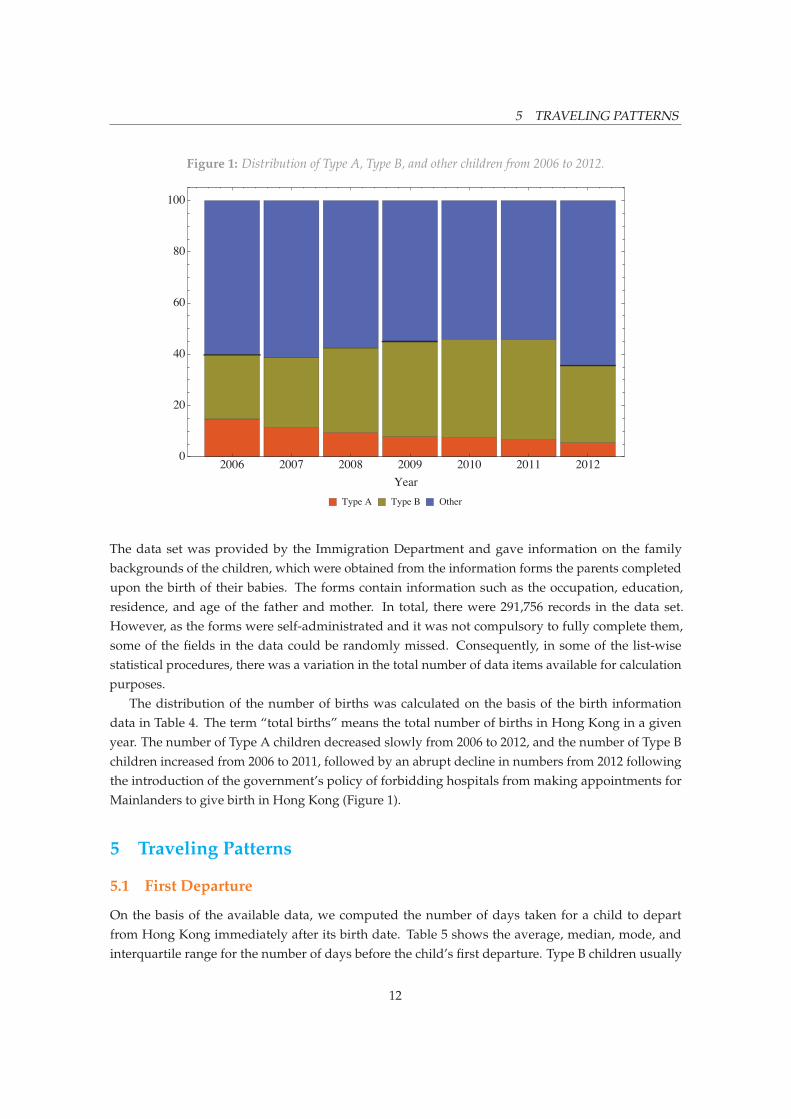
Figure 1: Distribution of Type A, Type B, and other children from 2006 to 2012.

The data set was provided by the Immigration Department and gave information on the familybackgrounds of the children, which were obtained from the information forms the parents completedupon the birth of their babies. The forms contain information such as the occupation, education,residence, and age of the father and mother. In total, there were 291,756 records in the data set.However, as the forms were self-administrated and it was not compulsory to fully complete them,some of the fields in the data could be randomly missed. Consequently, in some of the list-wisestatistical procedures, there was a variation in the total number of data items available for calculationpurposes.

The distribution of the number of births was calculated on the basis of the birth informationdata in Table 4. The term “total births” means the total number of births in Hong Kong in a givenyear. The number of Type A children decreased slowly from 2006 to 2012, and the number of Type Bchildren increased from 2006 to 2011, followed by an abrupt decline in numbers from 2012 followingthe introduction of the government’s policy of forbidding hospitals from making appointments forMainlanders to give birth in Hong Kong (Figure 1).

5 Traveling Patterns

5.1 First Departure

On the basis of the available data, we computed the number of days taken for a child to departfrom Hong Kong immediately after its birth date. Table 5 shows the average, median, mode, andinterquartile range for the number of days before the child’s first departure. Type B children usually

12

5.2 First Arrival 5 TRAVELING PATTERNS

leave Hong Kong earlier than Type A children.

Table 5: Statistics on the number of days between birth and first departure.

InterquartileMean Median Mode range

Type A 76 50 44 34Type B 26 23 29 16

5.2 First Arrival

The next arrival after the child’s first departure indicates the year of “first arrival” for each case (i.e.the first time a child comes back to Hong Kong after its first departure from the region).

Table 6 shows the distribution of first return observations for each child type and each year of birthacross different years.

Table 6: Percentage of first arrivals by cohort and year.

Year of Child Year of first arrival

birth type 2004 2005 2006 2007 2008 2009 2010 2011 2012 2013 2014

2004 A 47.9 46.3 3.2 1.9 0.3 0.1 0.1 0 0 0 0B 21.5 48.9 11.3 16.1 1.1 0.8 0 0 0 0 0

2005 A 63.7 30.7 3.0 1.6 0.3 0.2 0.1 0.1 0.1 0B 40.3 33.2 10.4 15.1 0.4 0.2 0.2 0 0.0 0.0

2006 A 70.7 24.6 2.5 1.5 0.1 0.2 0.1 0.0 0.0B 49.5 24.0 8.4 16.8 0.3 0.5 0.1 0.0 0.0

2007 A 72.2 22.5 2.8 1.6 0.2 0.2 0.1 0.0B 53.7 22.1 7.7 14.9 0.4 0.5 0.1 0.0

2008 A 72.3 22.6 2.8 1.5 0.2 0.1 0.0B 52.7 19.1 8.5 17.7 0.4 0.8 0.1

2009 A 73.6 21.5 2.8 1.5 0.2 0.0B 48.0 18.5 9.2 21.0 0.7 0.5

2010 A 70.1 25.5 2.4 1.5 0.1B 47.3 16.7 10.3 21.6 0.3

2011 A 77.2 18.9 2.2 0.6B 48.3 14.5 11.0 11.9

2012 A 71.6 24.0 1.0B 50.2 14.3 3.2

2013 A 74.7 17.1B 56.9 12.9

13

6.2 Return Rate by Mother’s Occupation 6 RETURN RATES

6 Return Rates

6.1 Return Rates by Ages and Birth Cohorts

According to the C&SD’s definition, a child is counted as having “returned” to Hong Kong if she/hestayed in Hong Kong for at least one month (31 nights, not necessarily consecutive) during the 6-monthperiod either before or after mid-year (i.e. 30 June of each year). For each child, we computed thenumber of nights she/he stayed in Hong Kong for each year and considered the child as havingreturned to Hong Kong if she/he stayed in Hong Kong for at least one month in either the first orsecond half of the year. Those cases that already live in Hong Kong are considered as “returned”.Table 7 shows the cumulative percentage of children who returned to Hong Kong at different ages.The cumulative percentage is calculated for age 1 and above.

Table 7: Cumulative return rate of Type A and Type B children at each age by birth cohort.

Year of Child Age of child

birth type 1 2 3 4 5 6 7 8 9

2004/2005 A 74.6 80.0 85.2 88.6 90.8 92.6 93.4 94.1 95.1B 37.6 39.5 43.0 45.5 48.1 50.7 52.5 53.9 56.2

2005/2006 A 73.4 78.4 82.6 87.0 89.1 91.2 92.5 93.3B 23.0 24.7 27.2 30.0 32.0 34.9 37.8 39.9

2006/2007 A 65.4 72.5 78.8 83.4 86.2 88.7 90.3B 9.3 11.3 14.4 17.0 19.9 24.0 27.5

2007/2008 A 64.7 71.3 77.6 82.0 84.4 87.3B 6.1 7.7 10.6 13.4 16.3 20.6

2008/2009 A 64.4 70.7 77.5 82.1 84.8B 5.3 6.8 9.6 12.8 16.2

2009/2010 A 60.7 68.9 75.7 80.8B 5.6 7.1 10.7 14.6

2010/2011 A 60.4 68.1 75.8B 4.6 6.2 10.4

2011/2012 A 58.3 67.2B 9.7 11.6

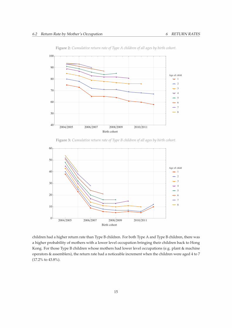
By looking at each column of Table 7, we can see the percentage of children returning to Hong Kongdecreasing for almost all ages. Figures 2 and 3 show this trend for Type A and B children, respectively.The decreasing return rate for Type B children is more rapid compared with that of Type A children.

6.2 Return Rate by Mother’s Occupation

Table 8 shows the return rates based on mother’s occupation and indicates whether the children hadreturned to Hong Kong at least once before the specified age. For all occupations of mothers, Type A

14

6.2 Return Rate by Mother’s Occupation 6 RETURN RATES

Figure 2: Cumulative return rate of Type A children of all ages by birth cohort.

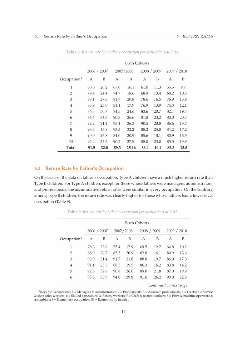
/ / / /Figure 3: Cumulative return rate of Type B children of all ages by birth cohort.

/ / / /

children had a higher return rate than Type B children. For both Type A and Type B children, there wasa higher probability of mothers with a lower level occupation bringing their children back to HongKong. For those Type B children whose mothers had lower level occupations (e.g. plant & machineoperators & assemblers), the return rate had a noticeable increment when the children were aged 4 to 7(17.2% to 43.8%).

15

6.3 Return Rate by Father’s Occupation 6 RETURN RATES

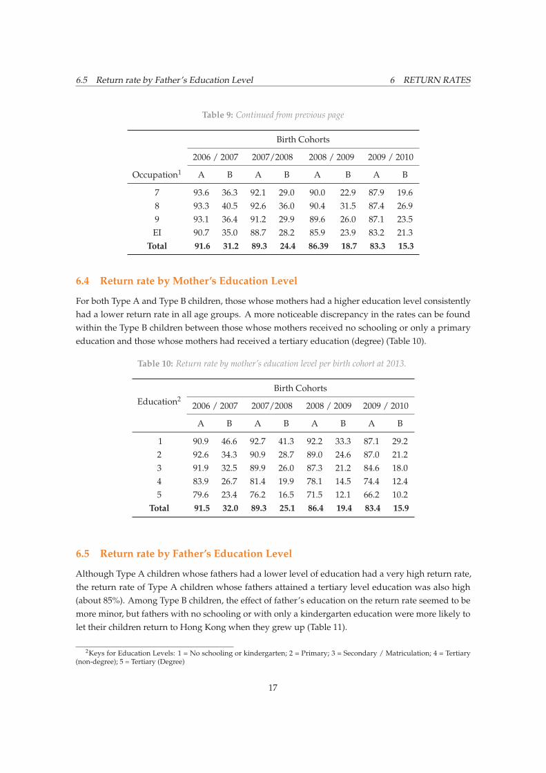
Table 8: Return rate by mother’s occupation per birth cohort at 2014.

Birth Cohorts

2006 / 2007 2007/2008 2008 / 2009 2009 / 2010

Occupation1 A B A B A B A B

1 68.6 20.2 67.0 16.1 61.0 11.3 55.5 9.72 79.4 24.4 74.7 18.6 68.9 13.4 68.2 10.53 89.1 27.6 81.7 20.8 78.6 16.5 76.9 13.84 85.9 23.0 81.1 17.9 76.9 13.9 74.3 12.15 86.3 30.7 84.5 24.6 83.6 20.7 82.1 19.46 86.4 34.3 90.3 26.6 81.8 23.2 80.0 20.77 92.9 31.1 95.1 26.3 90.5 20.8 86.6 19.78 93.3 43.8 93.3 32.2 88.2 25.0 84.2 17.29 90.0 26.8 84.0 20.9 85.6 18.1 80.9 16.5EI 92.2 34.2 90.2 27.5 88.0 23.0 85.5 19.9

Total 91.5 32.0 89.3 25.16 86.4 19.4 83.3 15.8

6.3 Return Rate by Father’s Occupation

On the basis of the data on father’s occupation, Type A children have a much higher return rate thanType B children. For Type A children, except for those whose fathers were managers, administrators,and professionals, the accumulative return rates were similar in every occupation. On the contrary,among Type B children, the return rate was clearly higher for those whose fathers had a lower leveloccupation (Table 9).

Table 9: Return rate by father’s occupation per birth cohort at 2013.

Birth Cohorts

2006 / 2007 2007/2008 2008 / 2009 2009 / 2010


1 78.3 23.0 75.4 17.9 69.5 12.7 64.8 10.22 88.9 26.7 85.5 20.9 82.8 16.1 80.9 13.63 93.9 31.4 91.7 21.8 88.8 19.7 86.0 17.34 91.1 25.3 88.5 19.5 86.3 16.2 83.8 14.25 92.8 32.6 90.8 26.0 89.0 21.8 87.0 19.96 95.5 33.9 94.0 29.8 91.6 26.2 90.0 22.3

Continued on next page1Keys for Occupations: 1 = Managers & Administrators; 2 = Professionals; 3 = Associate professionals; 4 = Clerks; 5 = Service

& shop sales workers; 6 = Skilled agricultural & fishery workers; 7 = Craft & related workers; 8 = Plant & machine operators &assemblers; 9 = Elementary occupation; EI = Economically inactive

16

6.5 Return rate by Father’s Education Level 6 RETURN RATES


Birth Cohorts

2006 / 2007 2007/2008 2008 / 2009 2009 / 2010


7 93.6 36.3 92.1 29.0 90.0 22.9 87.9 19.68 93.3 40.5 92.6 36.0 90.4 31.5 87.4 26.99 93.1 36.4 91.2 29.9 89.6 26.0 87.1 23.5EI 90.7 35.0 88.7 28.2 85.9 23.9 83.2 21.3

Total 91.6 31.2 89.3 24.4 86.39 18.7 83.3 15.3

6.4 Return rate by Mother’s Education Level

For both Type A and Type B children, those whose mothers had a higher education level consistentlyhad a lower return rate in all age groups. A more noticeable discrepancy in the rates can be foundwithin the Type B children between those whose mothers received no schooling or only a primaryeducation and those whose mothers had received a tertiary education (degree) (Table 10).

Table 10: Return rate by mother’s education level per birth cohort at 2013.

Education2Birth Cohorts

2006 / 2007 2007/2008 2008 / 2009 2009 / 2010

A B A B A B A B

1 90.9 46.6 92.7 41.3 92.2 33.3 87.1 29.22 92.6 34.3 90.9 28.7 89.0 24.6 87.0 21.23 91.9 32.5 89.9 26.0 87.3 21.2 84.6 18.04 83.9 26.7 81.4 19.9 78.1 14.5 74.4 12.45 79.6 23.4 76.2 16.5 71.5 12.1 66.2 10.2

Total 91.5 32.0 89.3 25.1 86.4 19.4 83.4 15.9

6.5 Return rate by Father’s Education Level

Although Type A children whose fathers had a lower level of education had a very high return rate,the return rate of Type A children whose fathers attained a tertiary level education was also high(about 85%). Among Type B children, the effect of father’s education on the return rate seemed to bemore minor, but fathers with no schooling or with only a kindergarten education were more likely tolet their children return to Hong Kong when they grew up (Table 11).

2Keys for Education Levels: 1 = No schooling or kindergarten; 2 = Primary; 3 = Secondary / Matriculation; 4 = Tertiary(non-degree); 5 = Tertiary (Degree)

17

6.6 Estimation of Return Rate for the Coming Years 6 RETURN RATES

Table 11: Return rate by father’s education level per birth cohort at 2013.

Education2Birth Cohorts

2006 / 2007 2007/2008 2008 / 2009 2009 / 2010A B A B A B A B

1 100.0 26.5 98.7 23.2 98.9 20.0 93.9 18.72 91.5 33.5 89.6 28.0 86.9 23.8 84.2 20.83 92.3 31.9 90.5 25.5 88.1 20.6 85.6 17.64 85.5 26.3 81.0 20.1 78.5 14.9 75.0 12.55 84.8 24.6 81.6 17.8 76.4 12.7 71.5 10.5

Total 91.6 31.2 89.3 24.4 86.4 18.7 83.4 15.4

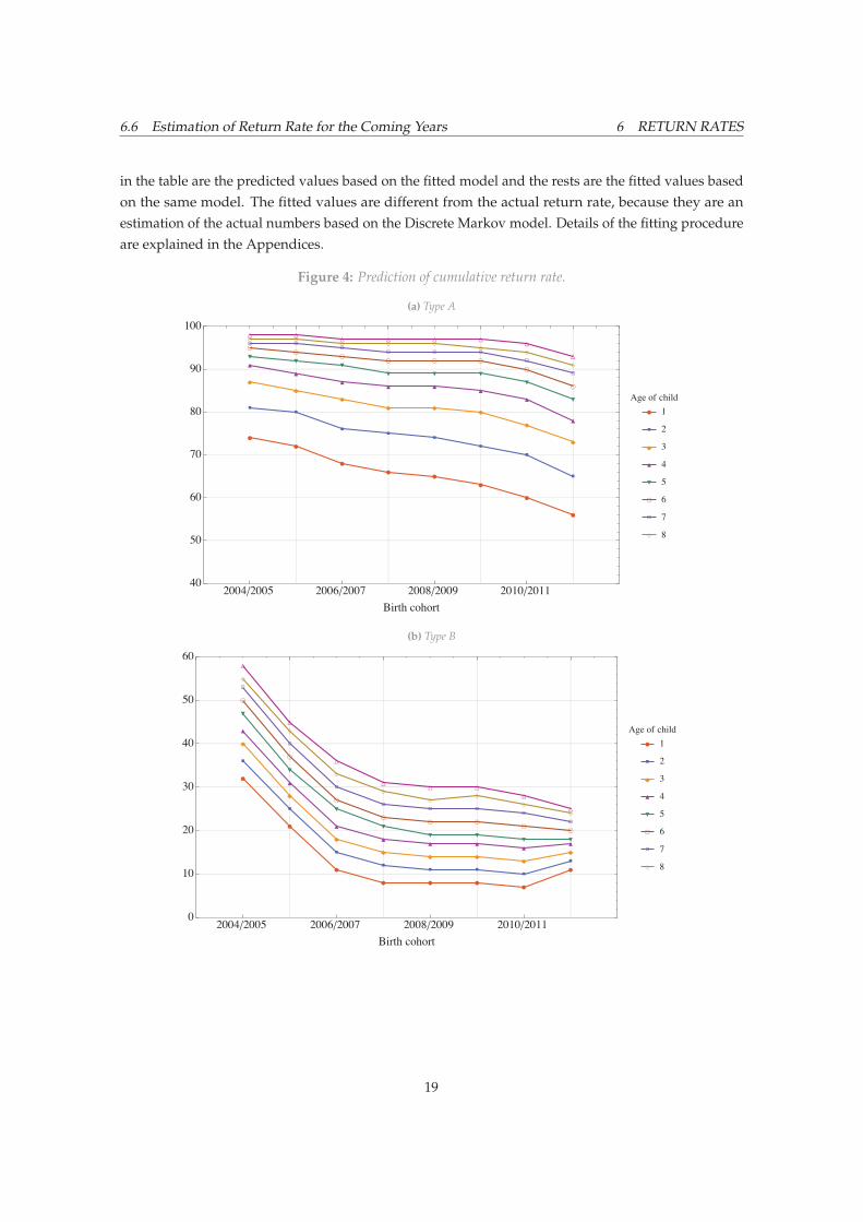
6.6 Estimation of Return Rate for the Coming Years

We fitted a discrete Markov chain model (Anderson and Goodman(1957) and Ching and Ng(2006)) tothe data points for each birth date category. We used maximum likelihood to estimate the model’sparameters. When the model was fitted, we simulated 1,000,000 realizations of the model to predictthe percentage of returned children in each year.

Table 12: Estimation of cumulative return rate by the Markov chain.

Date of Baby Age of child

birth type 1 2 3 4 5 6 7 8 9

2004/2005 A 74.3 81.5 86.8 90.5 93.1 95.1 96.4 97.4 98.1B 32.1 36.1 39.7 43.2 46.5 49.7 52.6 55.4 57.9

2005/2006 A 72.3 79.9 85.3 89.3 92.2 94.4 95.9 97.1 97.8

B 20.9 24.5 28.0 31.2 34.4 37.2 40.0 42.7 45.3

2006/2007 A 67.8 76.2 82.5 87.2 90.5 92.9 94.8 96.2 97.2

B 11.1 14.7 18.1 21.4 24.5 27.5 30.5 33.2 35.9

2007/2008 A 66.2 74.7 81.0 85.8 89.4 92.1 94.0 95.5 96.6

B 8.4 11.6 14.7 17.6 20.5 23.3 26.1 28.7 31.2

2008/2009 A 65.2 74.1 80.7 85.6 89.4 92.2 94.2 95.7 96.8

B 7.7 10.8 13.8 16.7 19.5 22.2 24.8 27.2 29.6

2009/2010 A 62.8 72.3 79.6 84.9 88.8 91.7 93.8 95.5 96.6

B 7.8 11.0 13.9 16.8 19.4 22.1 24.8 27.5 30.0

2010/2011 A 60.1 69.7 77.1 82.6 86.8 90.0 92.4 94.2 95.7

B 6.8 9.9 12.9 15.7 18.5 21.1 23.6 26.1 28.5

2011/2012 A 55.9 65.2 72.5 78.2 82.7 86.3 89.1 91.3 93.1

B 10.6 12.7 14.6 16.6 18.4 20.2 22.0 23.7 25.5

Table 12 and Figure 4 show the results of this fit for Type A and Type B children. The bold numbers

18

6.6 Estimation of Return Rate for the Coming Years 6 RETURN RATES

in the table are the predicted values based on the fitted model and the rests are the fitted values basedon the same model. The fitted values are different from the actual return rate, because they are anestimation of the actual numbers based on the Discrete Markov model. Details of the fitting procedureare explained in the Appendices.

Figure 4: Prediction of cumulative return rate.

(a) Type A

/ / / /(b) Type B

/ / / /

19

7 CROSS-BORDER STUDENTS

7 Cross-border Students

7.1 Estimation of Number of Cross-border Students

There is no variable in the data set to show if a case is the cross-border pupil or not, and thus it is notpossible to provide an exact number of these cases. We used the available information to estimate thenumber of such cases with some confidence. Cross-border students comprise of Type A and B babiesas well as ex-Hong Kong residents living in Shenzhen. Noted that the current study does not includethe latter.

We defined cross-border school pupils as those cases which arrived in Hong Kong and departedfrom Hong Kong on the same day during school seasons. On average, for each year, there areS0 = {8, 0, 19, 21, 19, 13, 19, 15, 20, 14, 20, 20} school days from June to May, respectively. If the patternof a case was similar to S0 we assumed that she/he was a cross-border pupil. To compare the patternof a case to S0 we computed its Euclidean distance (Deza and Deza 2009) to S0 . To simplify themodel, for each month, we assumed cases where the child arrived in Hong Kong and departed fromHong Kong on the same days to be a uniform distribution and distributions in different months to beindependent. We used the Monte Carlo method to estimate the percentiles of the distribution of theEuclidean distance between S0 and a random pattern of staying in Hong Kong in different monthsand used these percentiles to assign a case to the cross-border pupil set. If a case belonged to the lowerpercentile, it was more probable that it belonged to the cross-border pupil set.

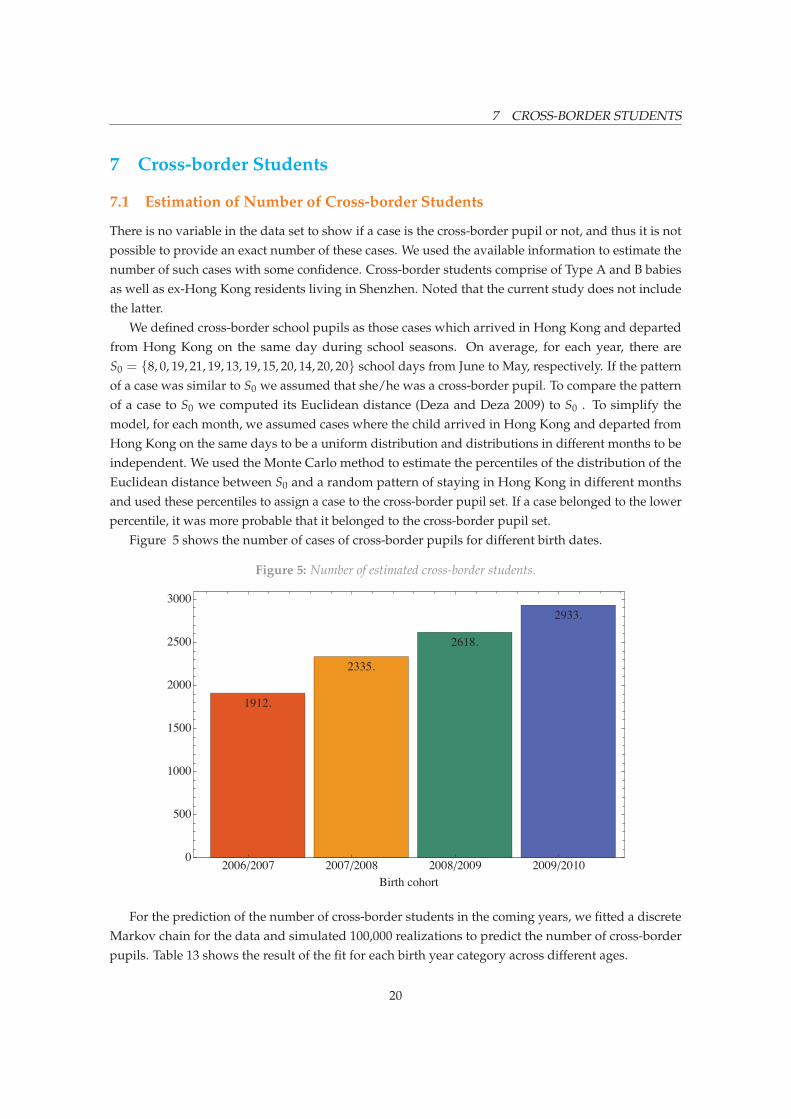
Figure 5 shows the number of cases of cross-border pupils for different birth dates.

Figure 5: Number of estimated cross-border students.

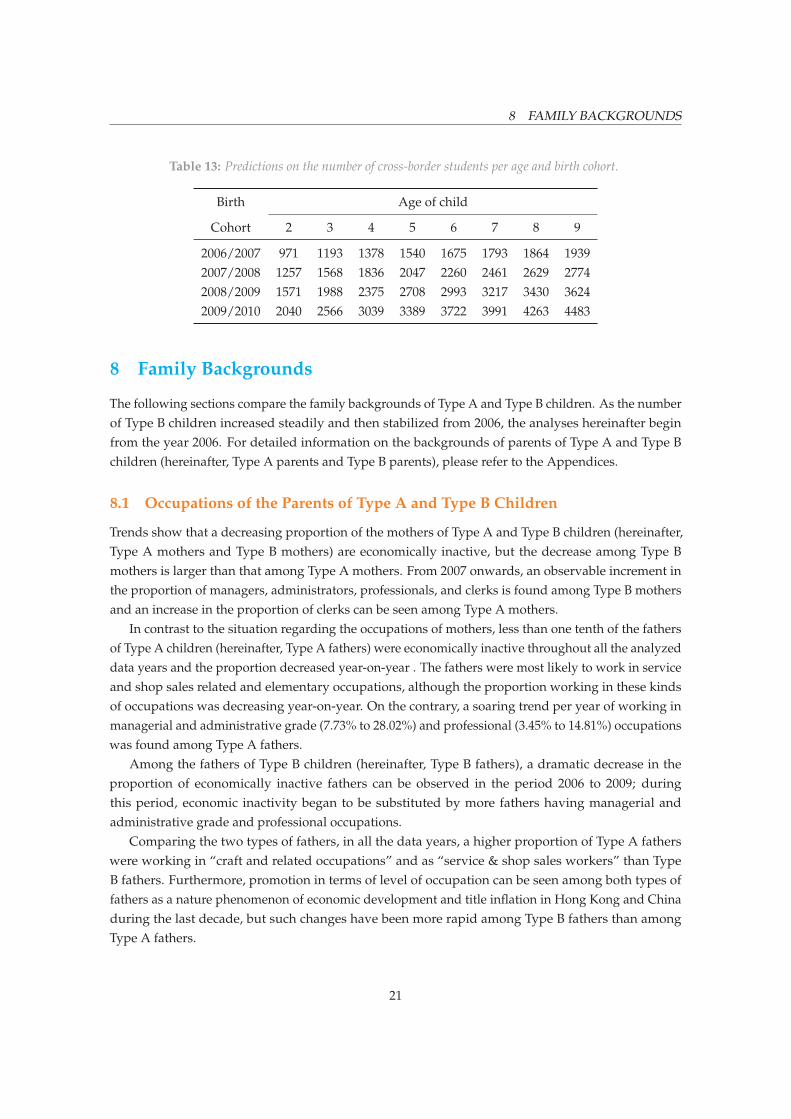
/ / / /For the prediction of the number of cross-border students in the coming years, we fitted a discrete

Markov chain for the data and simulated 100,000 realizations to predict the number of cross-borderpupils. Table 13 shows the result of the fit for each birth year category across different ages.

20

8 FAMILY BACKGROUNDS

Table 13: Predictions on the number of cross-border students per age and birth cohort.

Birth Age of child

Cohort 2 3 4 5 6 7 8 9

2006/2007 971 1193 1378 1540 1675 1793 1864 19392007/2008 1257 1568 1836 2047 2260 2461 2629 27742008/2009 1571 1988 2375 2708 2993 3217 3430 36242009/2010 2040 2566 3039 3389 3722 3991 4263 4483

8 Family Backgrounds

The following sections compare the family backgrounds of Type A and Type B children. As the numberof Type B children increased steadily and then stabilized from 2006, the analyses hereinafter beginfrom the year 2006. For detailed information on the backgrounds of parents of Type A and Type Bchildren (hereinafter, Type A parents and Type B parents), please refer to the Appendices.

8.1 Occupations of the Parents of Type A and Type B Children

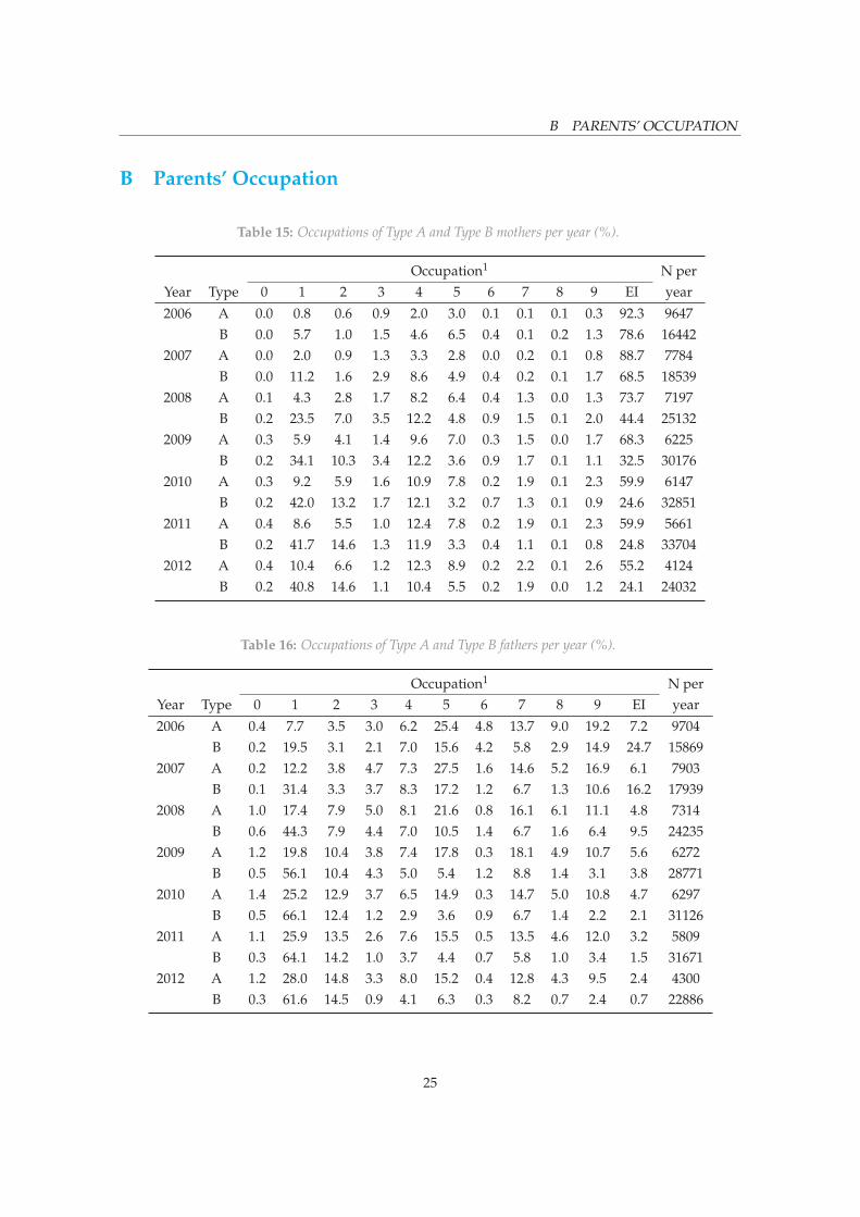
Trends show that a decreasing proportion of the mothers of Type A and Type B children (hereinafter,Type A mothers and Type B mothers) are economically inactive, but the decrease among Type Bmothers is larger than that among Type A mothers. From 2007 onwards, an observable increment inthe proportion of managers, administrators, professionals, and clerks is found among Type B mothersand an increase in the proportion of clerks can be seen among Type A mothers.

In contrast to the situation regarding the occupations of mothers, less than one tenth of the fathersof Type A children (hereinafter, Type A fathers) were economically inactive throughout all the analyzeddata years and the proportion decreased year-on-year . The fathers were most likely to work in serviceand shop sales related and elementary occupations, although the proportion working in these kindsof occupations was decreasing year-on-year. On the contrary, a soaring trend per year of working inmanagerial and administrative grade (7.73% to 28.02%) and professional (3.45% to 14.81%) occupationswas found among Type A fathers.

Among the fathers of Type B children (hereinafter, Type B fathers), a dramatic decrease in theproportion of economically inactive fathers can be observed in the period 2006 to 2009; duringthis period, economic inactivity began to be substituted by more fathers having managerial andadministrative grade and professional occupations.

Comparing the two types of fathers, in all the data years, a higher proportion of Type A fatherswere working in “craft and related occupations” and as “service & shop sales workers” than TypeB fathers. Furthermore, promotion in terms of level of occupation can be seen among both types offathers as a nature phenomenon of economic development and title inflation in Hong Kong and Chinaduring the last decade, but such changes have been more rapid among Type B fathers than amongType A fathers.

21

8.2 Education of Parents of Type A and Type B Children 8 FAMILY BACKGROUNDS

An examination of the marginal percentages of mother’s occupation by father’s occupation revealscombinations of fathers in managerial and administrative grade, professional, and associate profes-sional occupations with mothers in clerical grade or sales and related occupations among both TypeA and Type B parents. Nevertheless, it is more likely for Type B fathers’ spouses to have a clericaloccupation regardless of the father’s occupation.

8.2 Education of Parents of Type A and Type B Children

We found an increasing trend among both Type A and Type B mothers for a higher proportion of themto hold a tertiary degree , but a sharper increment was found among Type B mothers. The Type Amothers had usually attained a secondary school/matriculation qualification (consistent percentageof about 60% to 70% each year), whereas the proportion of Type B mothers acquiring a secondaryschool/matriculation qualification decreased from about 70% in 2006 to 37.4% in 2012.

22

Appendices

23

A NUMBER OF TYPE A AND TYPE I CHILDREN

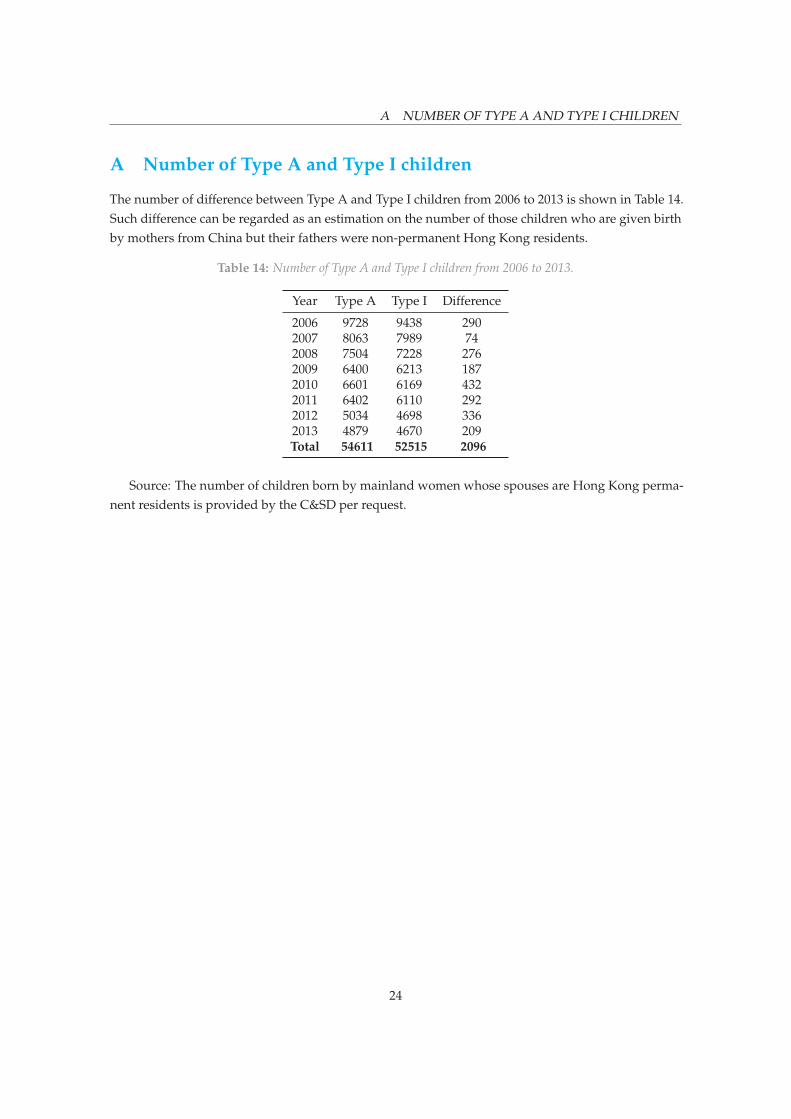
A Number of Type A and Type I children

The number of difference between Type A and Type I children from 2006 to 2013 is shown in Table 14.Such difference can be regarded as an estimation on the number of those children who are given birthby mothers from China but their fathers were non-permanent Hong Kong residents.

Table 14: Number of Type A and Type I children from 2006 to 2013.

Year Type A Type I Difference

2006 9728 9438 2902007 8063 7989 742008 7504 7228 2762009 6400 6213 1872010 6601 6169 4322011 6402 6110 2922012 5034 4698 3362013 4879 4670 209Total 54611 52515 2096

Source: The number of children born by mainland women whose spouses are Hong Kong perma-nent residents is provided by the C&SD per request.

24

B PARENTS’ OCCUPATION

B Parents’ Occupation

Table 15: Occupations of Type A and Type B mothers per year (%).

Occupation1 N perYear Type 0 1 2 3 4 5 6 7 8 9 EI year

2006 A 0.0 0.8 0.6 0.9 2.0 3.0 0.1 0.1 0.1 0.3 92.3 9647B 0.0 5.7 1.0 1.5 4.6 6.5 0.4 0.1 0.2 1.3 78.6 16442

2007 A 0.0 2.0 0.9 1.3 3.3 2.8 0.0 0.2 0.1 0.8 88.7 7784B 0.0 11.2 1.6 2.9 8.6 4.9 0.4 0.2 0.1 1.7 68.5 18539

2008 A 0.1 4.3 2.8 1.7 8.2 6.4 0.4 1.3 0.0 1.3 73.7 7197B 0.2 23.5 7.0 3.5 12.2 4.8 0.9 1.5 0.1 2.0 44.4 25132

2009 A 0.3 5.9 4.1 1.4 9.6 7.0 0.3 1.5 0.0 1.7 68.3 6225B 0.2 34.1 10.3 3.4 12.2 3.6 0.9 1.7 0.1 1.1 32.5 30176

2010 A 0.3 9.2 5.9 1.6 10.9 7.8 0.2 1.9 0.1 2.3 59.9 6147B 0.2 42.0 13.2 1.7 12.1 3.2 0.7 1.3 0.1 0.9 24.6 32851

2011 A 0.4 8.6 5.5 1.0 12.4 7.8 0.2 1.9 0.1 2.3 59.9 5661B 0.2 41.7 14.6 1.3 11.9 3.3 0.4 1.1 0.1 0.8 24.8 33704

2012 A 0.4 10.4 6.6 1.2 12.3 8.9 0.2 2.2 0.1 2.6 55.2 4124B 0.2 40.8 14.6 1.1 10.4 5.5 0.2 1.9 0.0 1.2 24.1 24032

Table 16: Occupations of Type A and Type B fathers per year (%).

Occupation1 N perYear Type 0 1 2 3 4 5 6 7 8 9 EI year

2006 A 0.4 7.7 3.5 3.0 6.2 25.4 4.8 13.7 9.0 19.2 7.2 9704B 0.2 19.5 3.1 2.1 7.0 15.6 4.2 5.8 2.9 14.9 24.7 15869

2007 A 0.2 12.2 3.8 4.7 7.3 27.5 1.6 14.6 5.2 16.9 6.1 7903B 0.1 31.4 3.3 3.7 8.3 17.2 1.2 6.7 1.3 10.6 16.2 17939

2008 A 1.0 17.4 7.9 5.0 8.1 21.6 0.8 16.1 6.1 11.1 4.8 7314B 0.6 44.3 7.9 4.4 7.0 10.5 1.4 6.7 1.6 6.4 9.5 24235

2009 A 1.2 19.8 10.4 3.8 7.4 17.8 0.3 18.1 4.9 10.7 5.6 6272B 0.5 56.1 10.4 4.3 5.0 5.4 1.2 8.8 1.4 3.1 3.8 28771

2010 A 1.4 25.2 12.9 3.7 6.5 14.9 0.3 14.7 5.0 10.8 4.7 6297B 0.5 66.1 12.4 1.2 2.9 3.6 0.9 6.7 1.4 2.2 2.1 31126

2011 A 1.1 25.9 13.5 2.6 7.6 15.5 0.5 13.5 4.6 12.0 3.2 5809B 0.3 64.1 14.2 1.0 3.7 4.4 0.7 5.8 1.0 3.4 1.5 31671

2012 A 1.2 28.0 14.8 3.3 8.0 15.2 0.4 12.8 4.3 9.5 2.4 4300B 0.3 61.6 14.5 0.9 4.1 6.3 0.3 8.2 0.7 2.4 0.7 22886

25

C COMBINATION OF PARENTS’ OCCUPATIONS

Figure 6: Occupations of Type A and Type B mothers per year (%).

= =

= =

= =

= =

= =

C Combination of Parents’ Occupations

From our observations of mother’s occupation by father’s occupation, we found a tendency amongboth Type A and Type B parents for fathers in managerial and administrative grade, professional,and associate professional occupations to be married to mothers in clerical grade or sales and relatedoccupations. Nevertheless, in all of the categories of father’s occupation, it is more likely that Type B

26


Figure 7: Occupations of Type A and Type B fathers per year (%).

= =

= =

= =

= =

= =

fathers might have spouses who have clerical occupations (Tables 17 and 18).In each crosstab of father’s and mother’s occupations (Tables 17 and 18), ignoring the negligible

figures in the category “armed forces & other occupations”, the triangle below the diagonal (the bluearea) indicates the combination of a father with a better occupation and a mother with a lower leveloccupation, the upper triangle over the diagonal (the orange area) indicates a combination of a fatherwith a lower level occupation and a mother with a better occupation, and the cases on the diagonal

27


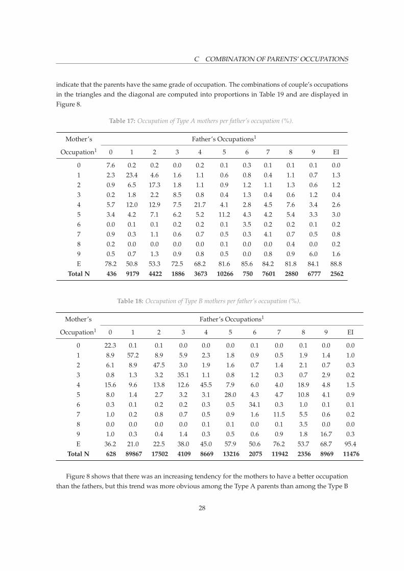
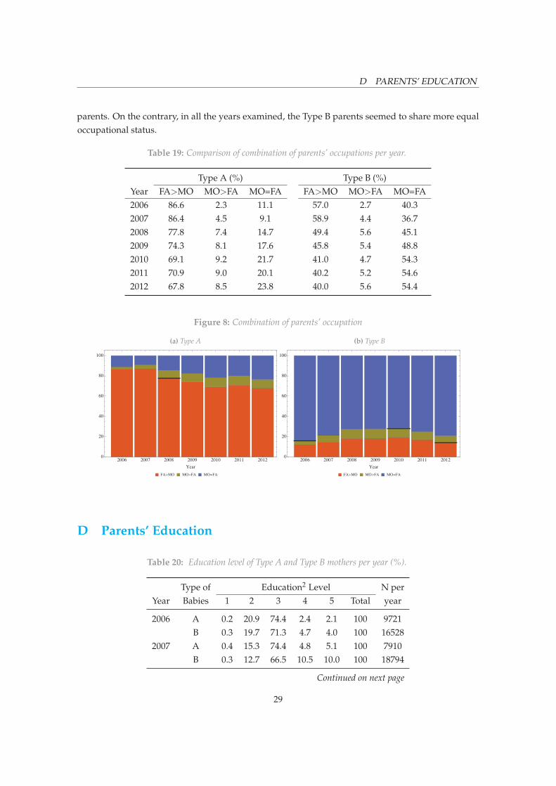
indicate that the parents have the same grade of occupation. The combinations of couple’s occupationsin the triangles and the diagonal are computed into proportions in Table 19 and are displayed inFigure 8.

Table 17: Occupation of Type A mothers per father’s occupation (%).

Mother’s Father’s Occupations1

Occupation1 0 1 2 3 4 5 6 7 8 9 EI

0 7.6 0.2 0.2 0.0 0.2 0.1 0.3 0.1 0.1 0.1 0.01 2.3 23.4 4.6 1.6 1.1 0.6 0.8 0.4 1.1 0.7 1.32 0.9 6.5 17.3 1.8 1.1 0.9 1.2 1.1 1.3 0.6 1.23 0.2 1.8 2.2 8.5 0.8 0.4 1.3 0.4 0.6 1.2 0.44 5.7 12.0 12.9 7.5 21.7 4.1 2.8 4.5 7.6 3.4 2.65 3.4 4.2 7.1 6.2 5.2 11.2 4.3 4.2 5.4 3.3 3.06 0.0 0.1 0.1 0.2 0.2 0.1 3.5 0.2 0.2 0.1 0.27 0.9 0.3 1.1 0.6 0.7 0.5 0.3 4.1 0.7 0.5 0.88 0.2 0.0 0.0 0.0 0.0 0.1 0.0 0.0 0.4 0.0 0.29 0.5 0.7 1.3 0.9 0.8 0.5 0.0 0.8 0.9 6.0 1.6E 78.2 50.8 53.3 72.5 68.2 81.6 85.6 84.2 81.8 84.1 88.8

Total N 436 9179 4422 1886 3673 10266 750 7601 2880 6777 2562

Table 18: Occupation of Type B mothers per father’s occupation (%).

Mother’s Father’s Occupations1

Occupation1 0 1 2 3 4 5 6 7 8 9 EI

0 22.3 0.1 0.1 0.0 0.0 0.0 0.1 0.0 0.1 0.0 0.01 8.9 57.2 8.9 5.9 2.3 1.8 0.9 0.5 1.9 1.4 1.02 6.1 8.9 47.5 3.0 1.9 1.6 0.7 1.4 2.1 0.7 0.33 0.8 1.3 3.2 35.1 1.1 0.8 1.2 0.3 0.7 2.9 0.24 15.6 9.6 13.8 12.6 45.5 7.9 6.0 4.0 18.9 4.8 1.55 8.0 1.4 2.7 3.2 3.1 28.0 4.3 4.7 10.8 4.1 0.96 0.3 0.1 0.2 0.2 0.3 0.5 34.1 0.3 1.0 0.1 0.17 1.0 0.2 0.8 0.7 0.5 0.9 1.6 11.5 5.5 0.6 0.28 0.0 0.0 0.0 0.0 0.1 0.1 0.0 0.1 3.5 0.0 0.09 1.0 0.3 0.4 1.4 0.3 0.5 0.6 0.9 1.8 16.7 0.3E 36.2 21.0 22.5 38.0 45.0 57.9 50.6 76.2 53.7 68.7 95.4

Total N 628 89867 17502 4109 8669 13216 2075 11942 2356 8969 11476

Figure 8 shows that there was an increasing tendency for the mothers to have a better occupationthan the fathers, but this trend was more obvious among the Type A parents than among the Type B

28

D PARENTS’ EDUCATION

parents. On the contrary, in all the years examined, the Type B parents seemed to share more equaloccupational status.

Table 19: Comparison of combination of parents’ occupations per year.

Type A (%) Type B (%)Year FA>MO MO>FA MO=FA FA>MO MO>FA MO=FA2006 86.6 2.3 11.1 57.0 2.7 40.32007 86.4 4.5 9.1 58.9 4.4 36.72008 77.8 7.4 14.7 49.4 5.6 45.12009 74.3 8.1 17.6 45.8 5.4 48.82010 69.1 9.2 21.7 41.0 4.7 54.32011 70.9 9.0 20.1 40.2 5.2 54.62012 67.8 8.5 23.8 40.0 5.6 54.4

Figure 8: Combination of parents’ occupation

(a) Type A

> > =

(b) Type B

> > =

D Parents’ Education

Table 20: Education level of Type A and Type B mothers per year (%).

Type of Education2 Level N perYear Babies 1 2 3 4 5 Total year

2006 A 0.2 20.9 74.4 2.4 2.1 100 9721B 0.3 19.7 71.3 4.7 4.0 100 16528

2007 A 0.4 15.3 74.4 4.8 5.1 100 7910B 0.3 12.7 66.5 10.5 10.0 100 18794


29

E COMBINATION OF PARENTS’ EDUCATION LEVELS



2008 A 0.3 13.8 68.8 9.7 7.4 100 7336B 0.2 7.1 53.0 20.0 19.7 100 25410

2009 A 0.2 9.9 70.2 12.0 7.7 100 6279B 0.1 4.4 45.3 25.3 24.9 100 30333

2010 A 0.2 7.9 66.0 14.4 11.5 100 6352B 0.1 2.9 36.4 28.9 31.7 100 33161

2011 A 0.1 7.4 64.3 16.3 12.0 100 5946B 0.1 2.3 34.5 26.5 36.5 100 34119

2012 A 0.1 4.5 62.4 16.4 16.6 100 4348B 0.1 0.6 37.4 21.8 40.1 100 24505

Table 21: Education level of Type A and Type B fathers per year (%).


2006 A 0.3 11.6 79.6 3.1 5.5 100 9706B 0.2 15.8 72.3 5.4 6.3 100 15879

2007 A 0.3 9.4 76.3 4.4 9.6 100 7915B 0.2 9.9 65.4 10.5 14.1 100 18001

2008 A 0.2 7.3 70.3 9.0 13.2 100 7340B 0.1 4.9 51.6 18.3 25.0 100 24322

2009 A 0.2 5.8 69.7 10.1 14.3 100 6282B 0.1 2.8 43.9 23.0 30.2 100 28831

2010 A 0.2 3.9 63.5 14.8 17.6 100 6349B 0.1 1.2 33.2 28.0 37.5 100 31232

2011 A 0.2 3.1 64.0 13.9 18.8 100 5935B 0.1 1.0 32.5 23.7 42.7 100 31904

2012 A 0.1 1.9 57.1 16.3 24.6 100 4382B 0.1 0.5 34.4 19.8 45.2 100 22991

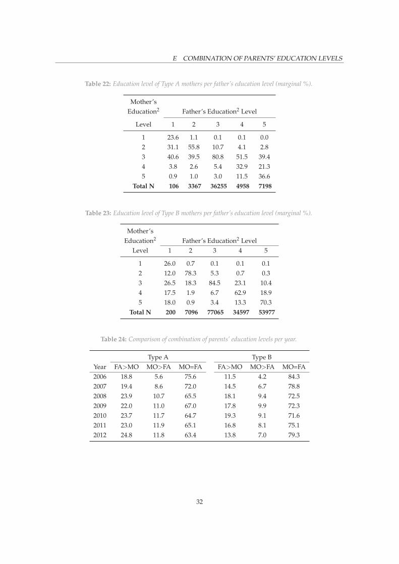
E Combination of Parents’ Education Levels

In both the Type A and the Type B cases, quite a high proportion of the children had parents whohad both completed secondary/matriculation level education (Figure 10). Comparing the level ofeducation between mothers and fathers, the parents of Type A and Type B children present quitedifferent trends. Although the data show a high proportion of parents having the same education

30


Figure 9: Education level of parents of Type A and Type B children (%).

= =

= / = /

= ( - ) = ( - )

= ( ) = ( )

qualification level among both Type A and Type B parents (Table 24, Figure 10), the proportion in TypeB is consistently higher than that in Type A throughout all the data years.

31


Table 22: Education level of Type A mothers per father’s education level (marginal %).

Mother’sEducation2 Father’s Education2 Level

Level 1 2 3 4 5

1 23.6 1.1 0.1 0.1 0.02 31.1 55.8 10.7 4.1 2.83 40.6 39.5 80.8 51.5 39.44 3.8 2.6 5.4 32.9 21.35 0.9 1.0 3.0 11.5 36.6

Total N 106 3367 36255 4958 7198

Table 23: Education level of Type B mothers per father’s education level (marginal %).

Mother’sEducation2 Father’s Education2 Level

Level 1 2 3 4 5

1 26.0 0.7 0.1 0.1 0.12 12.0 78.3 5.3 0.7 0.33 26.5 18.3 84.5 23.1 10.44 17.5 1.9 6.7 62.9 18.95 18.0 0.9 3.4 13.3 70.3

Total N 200 7096 77065 34597 53977

Table 24: Comparison of combination of parents’ education levels per year.

Type A Type BYear FA>MO MO>FA MO=FA FA>MO MO>FA MO=FA2006 18.8 5.6 75.6 11.5 4.2 84.32007 19.4 8.6 72.0 14.5 6.7 78.82008 23.9 10.7 65.5 18.1 9.4 72.52009 22.0 11.0 67.0 17.8 9.9 72.32010 23.7 11.7 64.7 19.3 9.1 71.62011 23.0 11.9 65.1 16.8 8.1 75.12012 24.8 11.8 63.4 13.8 7.0 79.3

32

F AGE OF CHILDBEARING

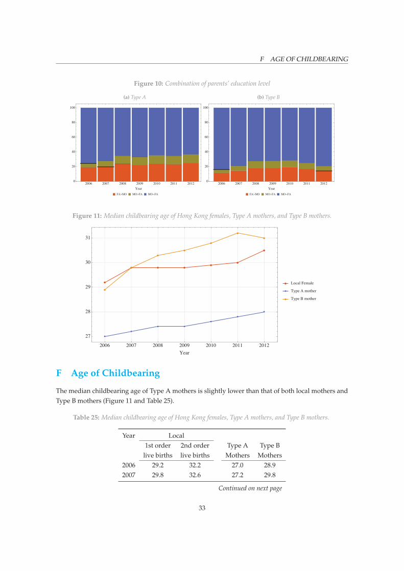
Figure 10: Combination of parents’ education level

(a) Type A

> > =

(b) Type B

> > =

Figure 11: Median childbearing age of Hong Kong females, Type A mothers, and Type B mothers.

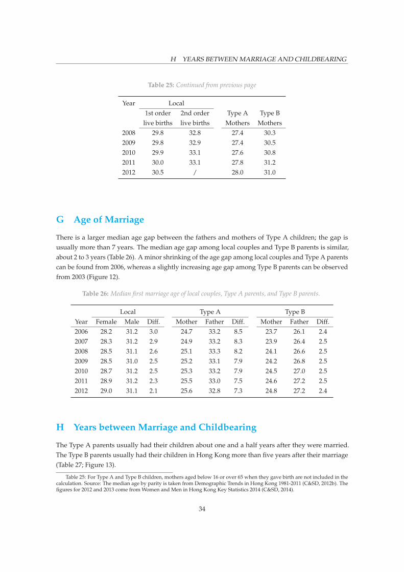
F Age of Childbearing

The median childbearing age of Type A mothers is slightly lower than that of both local mothers andType B mothers (Figure 11 and Table 25).

Table 25: Median childbearing age of Hong Kong females, Type A mothers, and Type B mothers.

Year Local1st order 2nd order Type A Type B

live births live births Mothers Mothers2006 29.2 32.2 27.0 28.92007 29.8 32.6 27.2 29.8


33

H YEARS BETWEEN MARRIAGE AND CHILDBEARING


Year Local1st order 2nd order Type A Type B

live births live births Mothers Mothers2008 29.8 32.8 27.4 30.32009 29.8 32.9 27.4 30.52010 29.9 33.1 27.6 30.82011 30.0 33.1 27.8 31.22012 30.5 / 28.0 31.0

G Age of Marriage

There is a larger median age gap between the fathers and mothers of Type A children; the gap isusually more than 7 years. The median age gap among local couples and Type B parents is similar,about 2 to 3 years (Table 26). A minor shrinking of the age gap among local couples and Type A parentscan be found from 2006, whereas a slightly increasing age gap among Type B parents can be observedfrom 2003 (Figure 12).

Table 26: Median first marriage age of local couples, Type A parents, and Type B parents.

Local Type A Type BYear Female Male Diff. Mother Father Diff. Mother Father Diff.2006 28.2 31.2 3.0 24.7 33.2 8.5 23.7 26.1 2.42007 28.3 31.2 2.9 24.9 33.2 8.3 23.9 26.4 2.52008 28.5 31.1 2.6 25.1 33.3 8.2 24.1 26.6 2.52009 28.5 31.0 2.5 25.2 33.1 7.9 24.2 26.8 2.52010 28.7 31.2 2.5 25.3 33.2 7.9 24.5 27.0 2.52011 28.9 31.2 2.3 25.5 33.0 7.5 24.6 27.2 2.52012 29.0 31.1 2.1 25.6 32.8 7.3 24.8 27.2 2.4

H Years between Marriage and Childbearing

The Type A parents usually had their children about one and a half years after they were married.The Type B parents usually had their children in Hong Kong more than five years after their marriage(Table 27; Figure 13).

Table 25: For Type A and Type B children, mothers aged below 16 or over 65 when they gave birth are not included in thecalculation. Source: The median age by parity is taken from Demographic Trends in Hong Kong 1981-2011 (C&SD, 2012b). Thefigures for 2012 and 2013 come from Women and Men in Hong Kong Key Statistics 2014 (C&SD, 2014).

34

H YEARS BETWEEN MARRIAGE AND CHILDBEARING

Figure 12: Age differences within local couples (first marriage), Type A parents, and Type B parents.

Figure 13: Differences of median year between childbearing and marriage

Table 27: Differences of median year between childbearing and marriage.

Year Type A Type B2006 1.5 4.72007 1.5 5.32008 1.6 5.62009 1.5 5.52010 1.5 5.62011 1.6 5.72012 1.6 5.4

35

J DISCRETE MARKOV CHAIN

I Hospital of Birth

Overall, the data showed that Type A children were more likely to be born in non-private hospitals thanin private hospitals (Table 28: 51.73% versus 48.26%) whereas Type B children were more likely to beborn in private hospitals than in non-private hospitals (Table 28: 78.77 versus 21.03). Nevertheless, insuccessive years, both Type A and Type B parents tended to use private hospitals more and non-privatehospitals less as places to give birth.

Table 28: Types of hospital used to give birth (%).

Non-privatePrivate /Other

Year N % N %

Type A 2006 3850 39.6 5878 60.42007 3766 46.7 4296 53.32008 3481 46.4 4020 53.62009 2922 45.7 3478 54.42010 2971 45.0 3629 55.02011 3206 50.1 3196 49.92012 3801 75.5 1233 24.5Total 23997 48.3 25730 51.7

Type B 2006 10302 62.3 6228 37.72007 14595 76.0 4598 24.02008 19285 74.5 6600 25.52009 23862 78.0 6722 22.02010 26933 79.1 7115 20.92011 29776 80.6 7179 19.42012 25418 92.6 2031 7.4Total 150171 78.8 40473 21.0

J Discrete Markov Chain

Let Xn ∈ 0, 1, n = 0, 1, . . . be the “returned” status of a child at age n, where 0 stands for “not returned”and 1 stands for “returned”. We assume that the status of a child at age n + 1 only depends onhis/her status at age n (i.e. probability of changing the status for a child only depends on his/herprevious year’s status); Pr(Xn+1 = in+1 X0 = i1, . . . , Xn = in) = Pr(Xn+1 = in+1 Xn = in), whereij ∈ 0, 1, j = 0, .., n + 1, see Ching and Ng(2006). Pr(Xn+1 = 0 Xn = 0), Pr(Xn+1 = 0 Xn = 1),Pr(Xn+1 = 1 Xn = 0) and Pr(Xn+1 = 1 Xn = 1) respectively indicate the probability that a case is a“not-returned child” at age n + 1 given she/he did not return the previous year, the probability that acase is a “not-returned child” at age n + 1 given she/he returned the previous year, the probabilitythat a case is a “returned child” at age n + 1 given she/he did not return the previous year, and the

36


probability that a case is a “returned child” at age n + 1 given she/he returned the previous year.These probabilities are estimated on the basis of the return pattern of cases in the database, Andersonand Goodman(1957) and Craig and Sendi(2002). On the basis of these estimated probabilities, we cansimulate a chain of the status of a typical child at different ages. The prediction of the return rate foreach birth cohort is based on 1,000,000 simulations of the estimated model and the calculation of thereturn rate for these 1,000,000 realizations. We used a similar methodology for fitting and predictingcross-border pupils.

37


References

Anderson, T. W., & Goodman, L. A. (1957). Statistical inference about Markov chains: The Annals ofMathematical Statistics, 28(1), 89-110.

Census and Statistics Department, HKSAR. (2012a). Hong Kong Population Projection 2012-2041. HongKong: Demographic Statistics Section, Census and Statistics Department, HKSAR.

Census and Statistics Department, HKSAR. (2012b). Demographic Trends in Hong Kong 1981-2011.Hong Kong: Demographic Statistics Section, Census and Statistics Department, HKSAR.

Census and Statistics Department, HKSAR. (2014). Women and Men in Hong Kong Key Statistics2014. Hong Kong: Demographic Statistics Section, Census and Statistics Department, HKSAR.

Ching W, & Ng M (2006). Markov Chains: Models, Algorithms and Applications. International Se-ries in Operations Research & Management Science. Springer. ISBN 9780387293356.

Craig, B. A., & Sendi, P. P. (2002). Estimation of the transition matrix of a discrete-time Markovchain. Health Economics, 11(1), 33–42.

Deza, E, & Deza, M. M. (2009). Encyclopedia of Distances. Springer. p. 94.

38

Documents

2013 A8 005 13A Final Report Prof Yip - pico.gov.hk