2004 Fitting Lanchester Equations to the Battles of Kursk ... · 2004 Fitting Lanchester Equations to the ... Fitting Lanchester Equations to the Battles of Kursk and Ardennes

Calhoun: The NPS Institutional Archive

Faculty and Researcher Publications Faculty and Researcher Publications

2004

Fitting Lanchester Equations to the

Battles of Kursk and Ardennes

Lucas, Thomas W.

Wiley Periodicals, Inc.

Naval Research Logistics, Volume 51, pp. 95â 116, 2004

http://hdl.handle.net/10945/44169

Fitting Lanchester Equations to the Battlesof Kursk and Ardennes

Thomas W. Lucas,1 Turker Turkes2

1 Operations Research Department, Naval Postgraduate School, Monterey, California 93943

2 Turkish Army, Ankara, Turkey

Received 12 June 2001; revised 3 February 2003; accepted 6 June 2003

DOI 10.1002/nav.10101

Abstract: Lanchester equations and their extensions are widely used to calculate attrition inmodels of warfare. This paper examines how Lanchester models fit detailed daily data on thebattles of Kursk and Ardennes. The data on Kursk, often called the greatest tank battle in history,was only recently made available. A new approach is used to find the optimal parameter valuesand gain an understanding of how well various parameter combinations explain the battles. Itturns out that a variety of Lanchester models fit the data about as well. This explains whyprevious studies on Ardennes, using different minimization techniques and data formulations,have found disparate optimal fits. We also find that none of the basic Lanchester laws (i.e.,square, linear, and logarithmic) fit the data particularly well or consistently perform better thanthe others. This means that it does not matter which of these laws you use, for with the rightcoefficients you will get about the same result. Furthermore, no constant attrition coefficientLanchester law fits very well. The failure to find a good-fitting Lanchester model suggests thatit may be beneficial to look for new ways to model highly aggregated attrition. © 2003 WileyPeriodicals, Inc. Naval Research Logistics 51: 95–116, 2004.

Keywords: Lanchester equations; Battle of Kursk; combat models; attrition; model validation

1. INTRODUCTION

Combat models provide information that assists decision-makers in making and justifyingdecisions that involve the expenditure of billions of dollars and impact many lives. For example,the simulation Concepts Evaluation Model (CEM) was used to give senior Army leadershipinsight into potential courses of action in the planning of Desert Storm [1]. Attrition plays apivotal role in most combat models, particularly campaign-level simulations, such as CEM. Theattrition in CEM, and many other combat models, is based on extensions of the theory developedby Lanchester [11] (see also Osipov [14] and Taylor [17]). Due to a dearth of data, particularly

Correspondence to: T. W. Lucas ([email protected])

© 2003 Wiley Periodicals, Inc.

two-sided, time-phased data, the validity of Lanchester equations as a model of aggregateattrition remains in question. This research examines how well Lanchester equations fit the onlydetailed two-sided, time-phased combat data available. In particular, we look at how wellLanchester models describe the battles of Kursk and Ardennes. Moreover, we test whether anyone of the common variants of Lanchester’s equations fits the battles better than the others.

Lanchester hypothesized that force levels in combat could be characterized by a coupled setof differential equations. A generalized version of Lanchester equations, as described byBracken [2], is

B�t� � a�d or 1/d�R�t�pB�t�q, (1)

R�t� � b�1/d or d�B�t�pR�t�q, (2)

where

B(t) and R(t) are the Soviet (Blue) and German (Red) force levels at time t,B(t) and R(t) are the rates at which the Soviet and German force levels are changingat time t,a and b are constant attrition-rate parameters,d is a tactical parameter that adjusts the attrition to the defender by a factor of (d) andthe attacker by a factor of (1/d),p is the exponent parameter of the attacking force,q is the exponent parameter of the defending force.

This generalized Lanchester model has five parameters (a, b, d, p, and q). The model beginsat the start of the battle (t � 0) with initial force sizes B(0) and R(0). When solved numerically,the force levels are incrementally decreased according to the equations B(t � �t) � B(t) ��t B(t) and R(t � �t) � R(t) � �t R(t), until the battle ends. For us, the time step �t is setequal to one day (the data resolution) throughout the analysis.

Lanchester studied two versions of these equations. The condition p � q � 1 (or, moregenerally, when p � q � 0) yields Lanchester’s linear law. Here, the state equation relatingforce levels at time t is b(B(0) � B(t)) � a(R(0) � R(t)). Lanchester viewed this as adescription of combat under “ancient conditions.” That is, these are the equations that wouldresult from a series of one-on-one duels between homogeneous forces. The linear law is alsoconsidered a good model for indirect fire (sometimes called area-fire) weapons, such as artillery(see [17]). Lanchester contrasted this with combat under “modern conditions,” which is definedas p � 1, q � 0 (or, more generally, p � q � 1). The state equation for modern combat isb(B(0)2 � B(t)2) � a(R(0)2 � R(t)2). This formulation is known as Lanchester’s square law.Lanchester showed the added importance of force size (relative to force quality) if attritionfollows the square law. Specifically, Lanchester used his simple models to show “the principleof concentration” in modern combat. A third version, with p � 0, q � 1 (or, more generally,q � p � 1), is called the logarithmic law (see Peterson [15]). This formulation suggests thata force’s attrition is a function of its force size, rather than the opponent’s. The logarithmic lawis sometimes used to model losses due to equipment failure, desertion, disease, and othernonbattle losses.

There are important consequences for force structure, training, and battlefield tactics if one ofthe Lanchester laws turns out to be a good model of aggregate attrition. Specifically, in the linear

96 Naval Research Logistics, Vol. 51 (2004)

law, ability (as measured by the attrition parameters a and b) is as important as numbers. Somehave speculated that the linear law may turn out to be the “new modern conditions.” Inparticular, if a force can orchestrate the battle (perhaps by using information superiority andagile maneuvers), such that engagements are typically one-on-one, the force may be able to tradequantity for quality.

There are few detailed two-sided, time-phased databases of historical battles. Time-phaseddata are needed to estimate the five parameters for a battle because before- and after-battle data(i.e., two time periods) result in an overdetermined system of equations, with an infinite numberof solutions. Therefore, for any p and q, we can find a and b that fit perfectly. Thus, as Hartleyand Hembold [9] write: “Unless we are able to procure [two-sided, time-phased data] we willnot be able to validate the homogeneous square law (or any other attrition law).” Fortunately,thanks to the Center for Army Analysis (CAA) and the Dupuy Institute, detailed time-phaseddata on the World War II battles of Kursk and Ardennes have recently become available (see[3] and [5]).

The goal of this research is to enhance our understanding of highly aggregated attrition bystudying how homogeneous generalized Lanchester models fit the time-phased data on thebattles of Kursk and Ardennes. In particular, we want to see if any of the basic laws (square,linear, or logarithmic) stand out. A better understanding of aggregate attrition offers the promiseof enhancing the utility of our campaign-level simulations. We emphasize the battle of Kursk,as there have been several previous analyses of the Ardennes campaign. Section 2 reviews someof the very few Lanchester attrition studies using time-phased data. A brief overview of thebattle of Kursk is provided in Section 3. Section 4 presents and discusses the data on the battleof Kursk, and introduces a new method for looking at two-sided, time-phased combat data. InSection 5, this method is applied to the battle of Kursk data. Section 6 applies the method to thedata on the Ardennes campaign and explains why previous researchers came to differentconclusions. Section 7 examines some excursions; in particular, the effects of breaking the battleof Kursk into multiple phases, assessing differences, and fitting only the manpower data. Thefinal section summarizes the key findings.

2. PREVIOUS RESEARCH ON TIME-PHASED COMBAT DATA

This section reviews the previous studies on time-phased combat data that motivated thisresearch. Empirical quantitative validation studies of Lanchester equations involving time-phased data include: Bracken [2], Fricker [8], and Wiper, Pettit, and Young [20], on theArdennes campaign; Clemens [4] on the battle of Kursk; Hartley and Helmbold [9] on theInchon–Seoul campaign; and Engle on the battle of Iwo Jima [7]. The last two had reliabletime-phased data for only one side. The previous works on the Ardennes data are discussed insome detail because different authors, using the same data, found diverse parameter estimates.

Bracken [2] formulated four different models for the Ardennes campaign using Eqs. (1) and(2). By means of a constrained grid search, he estimated the parameters (a, b, d, p, q) for thefirst 10 days of the Ardennes campaign with and without the defensive parameter (d) for combatforces and for total forces. Among his conclusions, Bracken found that “the Lanchester linearequation fits the [Ardennes] campaign” and there is an “attacker advantage.”

Fricker [8] extended Bracken’s analysis of the Ardennes campaign by: (1) using linearregression to fit the data from the entire campaign (32 days) to logarithmically transformedversions of Bracken’s generalized Lanchester equations; (2) using air-sortie data; and (3)restructuring the data “to estimate initial force sizes that reflect all of the troops that eventuallyfought in the campaign and then subtract the casualty attrition from this total on a daily basis.”

97Lucas and Turkes: Lanchester Equations for the Battles of Kursk and Ardennes

Fricker found that neither the linear nor the square law fit well. He concludes that a force’slosses were more a function of its own forces than of its opponent’s forces, similar to thelogarithmic law. Fricker’s best fits occur with exponent parameter values of q that are quitelarge—unbelievably large, in fact. For example, one of his models yields a q of 4.6 and a p of0. This suggests that a force could reduce its casualty rate by a factor of 24 by sending half ofits troops home, without affecting the opponent’s casualty rate. Of course, this extrapolates waybeyond the range of the data. Note: Fricker also fit Bracken’s data by regression techniques,obtaining estimates of p and q, for the combat forces with the tactical parameter, of .43 and�.50, respectively.

Wiper, Pettit, and Young [20] used Bayesian methods to reexamine Bracken’s and Fricker’sArdennes data. Their model is more general in that it uses two defensive parameters, a separateone for each side. Using Gibbs sampling, they estimate several posterior quantities of interest,in particular the means of p and q. Normal distributions are used to quantify their prior on theparameters (note: they have an extra defensive parameter and additional parameters for thevariances) and the residual error. The prior on p and q is an informative one, specifically, ( p,q) is distributed as circular normal with mean (.5, .5) and variance �2 � .25. This prior, whichhas over a .9 probability of ( p, q) both being between 0 and 1, is consistent with theconventional wisdom of plausible values. Moreover, the prior places equal a priori probabilityon the logarithmic, linear, and square laws. The most probable prior values of p and q are theprior mean of (.5, .5). This prior also heavily discounts p and q values larger than 1.5, with ana priori probability of about 1 in 2000 of both p and q being greater than 1.5. Using the 10 daysof combat forces data that Bracken used, Wiper et al.’s estimated posterior mean on ( p, q) is(.51, .48)—almost equal to the prior mean. Using 32 days of Bracken’s combat forces data, theirestimated posterior mean on ( p, q) is (.27, .84). Furthermore, using Bayes factors, theyconclude that “the logarithmic law fits best [and] the linear laws cannot be rejected, but thesquare law does seem implausible.” Using Fricker’s data, and the same prior, the estimatedposterior mean on ( p, q) is (.69, 1.06). When the variance of the prior on ( p, q) is inflated bya factor of 200 (i.e., a much less informative prior, with �2 � 50), the posterior mean on ( p, q)shifts to (�0.08, 4.88)—close to what Fricker found. This shows that the conclusions dependcritically on the sharpness of the prior, as the mean of the original prior and the mode of thelikelihood are about 10 prior standard deviations (� � .5) apart.

Clemens [4] fit Eqs. (1) and (2), without the tactical parameter d, to the battle of Kursk. Heformatted the data as Bracken did and used two different estimation techniques: (1) linearregression on logarithmically transformed equations, and (2) a nonlinear fit to the originalequations, using a numerical Newton-Raphson algorithm. Clemens also found that none of theLanchester square, linear, or logarithmic laws fit very well. Furthermore, the different estimationtechniques gave dramatically divergent estimates of the parameters. Using Newton-Raphson, hisestimates were p � 0 and q � 1.62, while the linear regression gave estimates of p � 5.32and q � 3.63.

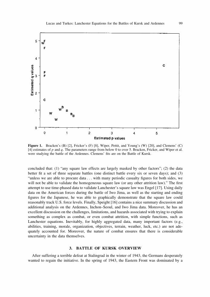
It is interesting to look across the breadth of Bracken’s [2], Fricker’s [8], Wiper et al.’s [20],and Clemens’ [4] findings. Figure 1 shows a scatter plot of the best-fitting p and q values thatthese authors found. The point here is to address the whole of the findings rather than thespecifics of the individual models. The only clear pattern that emerges from Figure 1 is that theestimates of p and q appear extremely sensitive to the different formulations and assumptions.Note: While Bracken’s fits are all close to the linear law, this is primarily due to his constrainedgrid search, which focused on parameters close to the linear law.

A couple of additional time-phased studies deserve mention. Hartley and Helmbold [9] testedLanchester’s square law using daily manpower numbers from the Inchon-Seoul campaign. They


concluded that: (1) “any square law effects are largely masked by other factors”; (2) the databetter fit a set of three separate battles (one distinct battle every six or seven days); and (3)“unless we are able to procure data . . . with many periodic casualty figures for both sides, wewill not be able to validate the homogeneous square law (or any other attrition law).” The firstattempt to use time-phased data to validate Lanchester’s square law was Engel [17]. Using dailydata on the American forces during the battle of Iwo Jima, as well as the starting and endingfigures for the Japanese, he was able to graphically demonstrate that the square law couldreasonably track U.S. force levels. Finally, Speight [16] contains a nice summary discussion andadditional analysis on the Ardennes, Inchon–Seoul, and Iwo Jima data. Moreover, he has anexcellent discussion on the challenges, limitations, and hazards associated with trying to explainsomething as complex as combat, or even combat attrition, with simple functions, such asLanchester equations. Inevitably, for highly aggregated data, many important factors (e.g.,abilities, training, morale, organization, objectives, terrain, weather, luck, etc.) are not ade-quately accounted for. Moreover, the nature of combat ensures that there is considerableuncertainty in the data themselves.

3. BATTLE OF KURSK OVERVIEW

After suffering a terrible defeat at Stalingrad in the winter of 1943, the Germans desperatelywanted to regain the initiative. In the spring of 1943, the Eastern Front was dominated by a

Figure 1. Bracken’s (B) [2], Fricker’s (F) [8], Wiper, Pettit, and Young’s (W) [20], and Clemens’ (C)[4] estimates of p and q. The parameters range from below 0 to over 5. Bracken, Fricker, and Wiper et al.were studying the battle of the Ardennes. Clemens’ fits are on the Battle of Kursk.


salient, 200 km wide and 150 km deep, centered on the city of Kursk. The Germans planned,in a classic pincer operation named Operation Citadel, to eliminate the salient and destroy theSoviet forces in it. On 2 July 1943, Hitler declared, “This attack is of decisive importance. Itmust succeed, and it must do so rapidly and convincingly. It must secure for us the initia-tive. . . . The victory of Kursk must be a blazing torch to the world.” [18]

After nearly 2 months of delays, Operation Citadel was launched on 5 July, with a two-frontattack on the Kursk salient. Due to good intelligence and the extra time that the Soviets had toget ready, the Germans attacked well-prepared positions. The attack on the northern front raninto stiff Soviet defenses and quickly bogged down. However, on the southern front of the battle,in heavy fighting, the Germans penetrated as much as 46 km by 12 July. This put the Germansin position to capture the town of Prokhorovka and establish a bridgehead over the Psel River,the last natural barrier between them and Kursk. To counter this, the Soviets deployed theirstrategic armored reserve, the 5th Guards Tank Army, under Lieutenant General Pavel Rotmis-trov. On the 12th, outside of Prokhorovka, the German’s II SS Panzer Corps, commanded by SSObergruppenfuehrer Paul Hausser, slammed into the advancing 5th Guards Tank Army. Theresult has been called the greatest armored engagement in history. On that day, the Germans lost98 tanks,1 while the Soviets lost 414 tanks. Although, in terms of casualties, Germany seemedto win the day, Hitler gave orders on 13 July to cancel Operation Citadel. For the rest of thebattle, the Germans assumed a generally defensive posture. Field Marshal Erich von Manstein,Commander of Army Group South, felt that “[stopping the offensive] at this moment [was]tantamount to throwing victory away [10].” By 23 July, Soviet counterattacks had regained allof the ground lost in the battle. As Manstein prophetically wrote “the last German offensive inthe East ended in a fiasco, even though the enemy . . . suffered four times their losses” (see [10]).More information about the battle of Kursk can be found in [3], [10], [18], and [22].

4. DATA AND ANALYSIS APPROACH

4.1 The Data

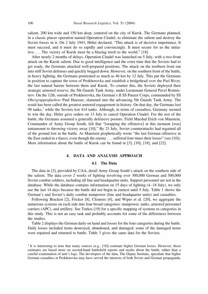
The data in [3], provided by CAA, detail Army Group South’s attack on the southern side ofthe salient. The data cover 2 weeks of fighting involving over 300,000 German and 500,000Soviet combat soldiers, including all line and headquarter units. Support personnel are not in thedatabase. While the database contains information on 15 days of fighting (4–18 July), we onlyuse the last 14 days because the battle did not begin in earnest until 5 July. Table 1 shows theGerman’s and Soviet’s daily combat manpower (line and headquarter units) and casualties.

Following Bracken [2], Fricker [8], Clemens [4], and Wiper et al. [20], we aggregate thenumerous systems on each side into four broad categories: manpower, tanks, armored personnelcarriers (APC), and artillery. See Turkes [19] for a specific mapping of systems to categories inthis study. This is not an easy task and probably accounts for some of the differences betweenthe studies.

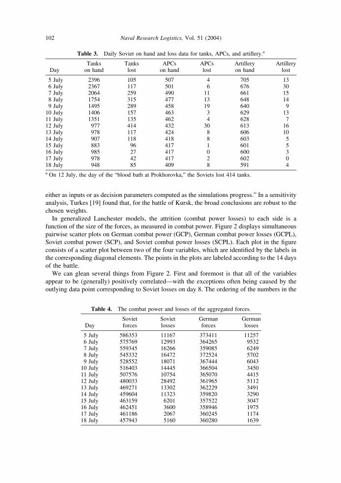
Table 2 displays the German daily on hand and losses for the four categories during the battle.Daily losses included items destroyed, abandoned, and damaged; some of the damaged itemswere repaired and returned to battle. Table 3 gives the same data for the Soviets.

1 It is interesting to note that many sources (e.g., [18]) estimate higher German losses. However, thoseestimates are based more on second-hand battlefield reports and myths about the battle, rather than acareful examination of unit’s logs. The developers of the data, The Depuy Institute, speculate that higherGerman casualties at Prokhorovka may have served the interests of both Soviet and German propaganda.


The data in Tables 1–3 classify the many combat systems in the battle into four broadcategories (manpower, tanks, APCs, and artillery). Even so, with only 14 days of data, there arenot enough degrees of freedom to fit heterogeneous Lanchester models—though Clemens [4],with additional assumptions (constraints), investigated aspects of heterogeneous models. Thus,like the authors above, we fit homogeneous models. Table 4 presents the data on the combatpower of the Soviet and German forces. The combat power of a force is defined as a weightedsum of combat manpower, APCs, tanks, and artillery, with weights of 1, 5, 20, and 40,respectively. These are the weights used in the previous studies. Bracken [2] writes that:“Virtually all theater-level dynamic combat simulation models incorporate similar weights,

Table 1. Combat manpower for both sides.a

DaySoviet

manpowerSoviet

casualtiesGerman

manpowerGerman

casualties

5 July 507698 8527 301341 61926 July 498884 9423 297205 43027 July 489175 10431 293960 34148 July 481947 9547 306659 29429 July 470762 11836 303879 2953

10 July 460808 10770 302014 204011 July 453126 7754 300050 247512 July 433813 19422 298710 261213 July 423351 10522 299369 205114 July 415254 8723 297395 214015 July 419374 4076 296237 132216 July 416666 2940 296426 135017 July 415461 1217 296350 94918 July 413298 3260 295750 1054a Casualties are those killed, wounded, captured/missing in action, and disease andnonbattle injuries. Daily force levels depend on previous force levels, casualties, andreinforcements. The attacking Germans are outnumbered.

Table 2. Daily German on hand and loss data for tanks, APCs, and artillery.a

DayTanks

on handTankslost

APCson hand

APCslost

Artilleryon hand

Artillerylost

5 July 986 198 1142 29 1166 246 July 749 248 1128 14 1161 57 July 673 121 1101 27 1154 78 July 596 108 1085 16 1213 139 July 490 139 1073 14 1210 6

10 July 548 36 1114 42 1199 1211 July 563 63 1104 16 1206 1512 July 500 98 1099 12 1194 1213 July 495 57 1096 4 1187 714 July 480 46 1093 6 1184 515 July 426 79 1089 5 1183 316 July 495 23 1092 1 1179 417 July 557 7 1095 1 1182 218 July 588 6 1098 5 1182 11a The Germans suffered their heaviest tank losses during the first 2 days of the battle, when they wereattacking heavily prepared defenses.


either as inputs or as decision parameters computed as the simulations progress.” In a sensitivityanalysis, Turkes [19] found that, for the battle of Kursk, the broad conclusions are robust to thechosen weights.

In generalized Lanchester models, the attrition (combat power losses) to each side is afunction of the size of the forces, as measured in combat power. Figure 2 displays simultaneouspairwise scatter plots on German combat power (GCP), German combat power losses (GCPL),Soviet combat power (SCP), and Soviet combat power losses (SCPL). Each plot in the figureconsists of a scatter plot between two of the four variables, which are identified by the labels inthe corresponding diagonal elements. The points in the plots are labeled according to the 14 daysof the battle.

We can glean several things from Figure 2. First and foremost is that all of the variablesappear to be (generally) positively correlated—with the exceptions often being caused by theoutlying data point corresponding to Soviet losses on day 8. The ordering of the numbers in the

Table 3. Daily Soviet on hand and loss data for tanks, APCs, and artillery.a

DayTanks

on handTankslost

APCson hand

APCslost

Artilleryon hand

Artillerylost

5 July 2396 105 507 4 705 136 July 2367 117 501 6 676 307 July 2064 259 490 11 661 158 July 1754 315 477 13 648 149 July 1495 289 458 19 640 9

10 July 1406 157 463 3 629 1311 July 1351 135 462 4 628 712 July 977 414 432 30 613 1613 July 978 117 424 8 606 1014 July 907 118 418 8 603 515 July 883 96 417 1 601 516 July 985 27 417 0 600 317 July 978 42 417 2 602 018 July 948 85 409 8 591 4a On 12 July, the day of the “blood bath at Prokhorovka,” the Soviets lost 414 tanks.

Table 4. The combat power and losses of the aggregated forces.

DaySovietforces

Sovietlosses

Germanforces

Germanlosses

5 July 586353 11167 373411 112576 July 575769 12993 364265 95327 July 559345 16266 359085 62498 July 545332 16472 372524 57029 July 528552 18071 367444 6043

10 July 516403 14445 366504 345011 July 507576 10754 365070 441512 July 480033 28492 361965 511213 July 469271 13302 362229 349114 July 459604 11323 359820 329015 July 463159 6201 357522 304716 July 462451 3600 358946 197517 July 461186 2067 360245 117418 July 457943 5160 360280 1639


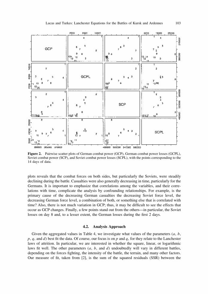
plots reveals that the combat forces on both sides, but particularly the Soviets, were steadilydeclining during the battle. Casualties were also generally decreasing in time, particularly for theGermans. It is important to emphasize that correlations among the variables, and their corre-lations with time, complicate the analysis by confounding relationships. For example, is theprimary cause of the decreasing German casualties the decreasing Soviet force level, thedecreasing German force level, a combination of both, or something else that is correlated withtime? Also, there is not much variation in GCP; thus, it may be difficult to see the effects thatoccur as GCP changes. Finally, a few points stand out from the others—in particular, the Sovietlosses on day 8 and, to a lesser extent, the German losses during the first 2 days.

4.2. Analysis Approach

Given the aggregated values in Table 4, we investigate what values of the parameters (a, b,p, q, and d) best fit the data. Of course, our focus is on p and q, for they relate to the Lanchesterlaws of attrition. In particular, we are interested in whether the square, linear, or logarithmiclaws fit well. The other parameters (a, b, and d) undoubtedly will vary in different battles,depending on the forces fighting, the intensity of the battle, the terrain, and many other factors.Our measure of fit, taken from [2], is the sum of the squared residuals (SSR) between the

Figure 2. Pairwise scatter plots of German combat power (GCP), German combat power losses (GCPL),Soviet combat power (SCP), and Soviet combat power losses (SCPL), with the points corresponding to the14 days of data.


estimated and actual attrition. The objective is to find the parameters that minimize SSR—i.e.,provide the best fit. Specifically, the objective function that we minimize is

SSR � �n�1

14

�Bn � a�d*n�RnpBn

q�2 � �n�1

14

�Rn � b�d*n�BnpRn

q�2, (3)

where

n indexes the 14 days of the battle,d*n � d if the side (Red or Blue) is on the defensive on day n and 1/d if the side ison the offensive. If neither or both sides are clearly on the offensive, then d*n � 1.

Rather than use a standard optimization method to find the parameters that minimize SSR,such as Bracken’s [2] constrained grid search, Fricker’s [8] linear regression on logarithmicallytransformed data, Wiper et al.’s [20] posterior maximum, or Clemens’ [4] numerical Newton-Raphson, we look at the best-fitting response surface as a function of p and q. Given p and q,it turns out to be relatively easy to find a, b, and d to minimize SSR. Our approach is as follows:For a fixed d, solve for a and b by regression through the origin (a simple analytic formulaexists; see [12] or [13]). Note: Bn, Rn, Bn, and Rn are known—thus, only a and b need to beestimated. This calculation is repeated for many values of d. Specifically, through a one-dimensional line search on d, we find the d, and associated a and b, that minimize SSR for thegiven p and q. By plotting the contours of the minimum SSR as a function of p and q, not onlycan we visually assess where the optimum occurs, but we also get a better understanding of howthe surface of Lanchester exponent parameters fits the battle.

5. LANCHESTER AND THE BATTLE OF KURSK

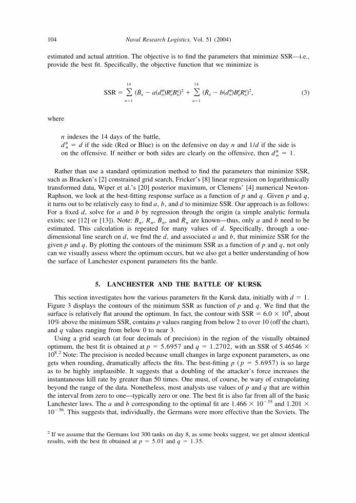
This section investigates how the various parameters fit the Kursk data, initially with d � 1.Figure 3 displays the contours of the minimum SSR as function of p and q. We find that thesurface is relatively flat around the optimum. In fact, the contour with SSR � 6.0 � 108, about10% above the minimum SSR, contains p values ranging from below 2 to over 10 (off the chart),and q values ranging from below 0 to near 3.

Using a grid search (at four decimals of precision) in the region of the visually obtainedoptimum, the best fit is obtained at p � 5.6957 and q � 1.2702, with an SSR of 5.46546 �108.2 Note: The precision is needed because small changes in large exponent parameters, as onegets when rounding, dramatically affects the fits. The best-fitting p ( p � 5.6957) is so largeas to be highly implausible. It suggests that a doubling of the attacker’s force increases theinstantaneous kill rate by greater than 50 times. One must, of course, be wary of extrapolatingbeyond the range of the data. Nonetheless, most analysts use values of p and q that are withinthe interval from zero to one—typically zero or one. The best fit is also far from all of the basicLanchester laws. The a and b corresponding to the optimal fit are 1.466 � 10�35 and 1.201 �10�36. This suggests that, individually, the Germans were more effective than the Soviets. The

2 If we assume that the Germans lost 300 tanks on day 8, as some books suggest, we get almost identicalresults, with the best fit obtained at p � 5.01 and q � 1.35.


optimal values of a and b are quite small, as they must be to balance the very high values of theoptimal exponent parameters p and q.

In addition to SSR, another measure of fit that we use is R2, where R2 � 1 � SSR/SST. SST,the sum squares total, is calculated by

SST � �n�1

14

�Bn � B� �2 � �n�1

14

�Rn � R� �2, (4)

with B� and R� denoting the mean daily force losses for the Soviets and Germans, respectively.Here, R2 is defined analogously to how it is in standard least squares regression and is a linearfunction of SSR. Larger R2 values correspond to better fits, with a perfect fit (i.e., an SSR � 0)yielding an R2 � 1. Note: In this setup, it is possible to get negative R2 values, which meansthat the fitted model yields worse results than using the average daily losses as estimates. Anadvantage of R2 over SSR is that it is invariant to linear transforms of the data. This allows usto compare models using different weights and data. In the best-fitting model above, the R2 is.237. That is, the model explains less than a quarter of the squared variation.

We can see how well the optimum parameter estimates fit the battle by examining the actualand estimated losses over the 14 days. Figures 4 and 5 show the actual and estimated Soviet and

Figure 3. A contour plot of the minimum SSR as a function of p and q, with the tactical parameter (d)not included (i.e., no attacker or defender advantage in this model). Note: The small wiggles and othernonsmooth features in this and the other contour plots are a function of the granularity of the points uponwhich the surface was evaluated and the software used to generate the plots. In all subregions that theauthors have zoomed in on, the contours are smooth.


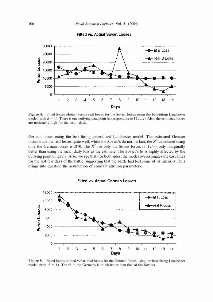
German losses using the best-fitting generalized Lanchester model. The estimated Germanlosses track the real losses quite well, while the Soviet’s do not. In fact, the R2 calculated usingonly the German forces is .870. The R2 for only the Soviet forces is .124—only marginallybetter than using the mean daily loss as the estimate. The Soviet’s fit is highly affected by theoutlying point on day 8. Also, we see that, for both sides, the model overestimates the casualtiesfor the last few days of the battle, suggesting that the battle had lost some of its intensity. Thisbrings into question the assumption of constant attrition parameters.

Figure 4. Fitted losses plotted versus real losses for the Soviet forces using the best-fitting Lanchestermodel (with d � 1). There is one outlying data point (corresponding to 12 July). Also, the estimated lossesare noticeably high for the last 4 days.

Figure 5. Fitted losses plotted versus real losses for the German forces using the best-fitting Lanchestermodel (with d � 1). The fit to the Germans is much better than that of the Soviets.


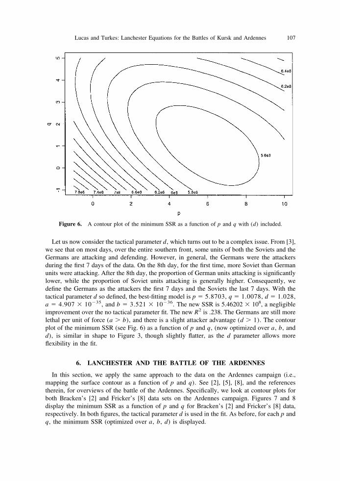
Let us now consider the tactical parameter d, which turns out to be a complex issue. From [3],we see that on most days, over the entire southern front, some units of both the Soviets and theGermans are attacking and defending. However, in general, the Germans were the attackersduring the first 7 days of the data. On the 8th day, for the first time, more Soviet than Germanunits were attacking. After the 8th day, the proportion of German units attacking is significantlylower, while the proportion of Soviet units attacking is generally higher. Consequently, wedefine the Germans as the attackers the first 7 days and the Soviets the last 7 days. With thetactical parameter d so defined, the best-fitting model is p � 5.8703, q � 1.0078, d � 1.028,a � 4.907 � 10�35, and b � 3.521 � 10�36. The new SSR is 5.46202 � 108, a negligibleimprovement over the no tactical parameter fit. The new R2 is .238. The Germans are still morelethal per unit of force (a � b), and there is a slight attacker advantage (d � 1). The contourplot of the minimum SSR (see Fig. 6) as a function of p and q, (now optimized over a, b, andd), is similar in shape to Figure 3, though slightly flatter, as the d parameter allows moreflexibility in the fit.

6. LANCHESTER AND THE BATTLE OF THE ARDENNES

In this section, we apply the same approach to the data on the Ardennes campaign (i.e.,mapping the surface contour as a function of p and q). See [2], [5], [8], and the referencestherein, for overviews of the battle of the Ardennes. Specifically, we look at contour plots forboth Bracken’s [2] and Fricker’s [8] data sets on the Ardennes campaign. Figures 7 and 8display the minimum SSR as a function of p and q for Bracken’s [2] and Fricker’s [8] data,respectively. In both figures, the tactical parameter d is used in the fit. As before, for each p andq, the minimum SSR (optimized over a, b, d) is displayed.

Figure 6. A contour plot of the minimum SSR as a function of p and q with (d) included.


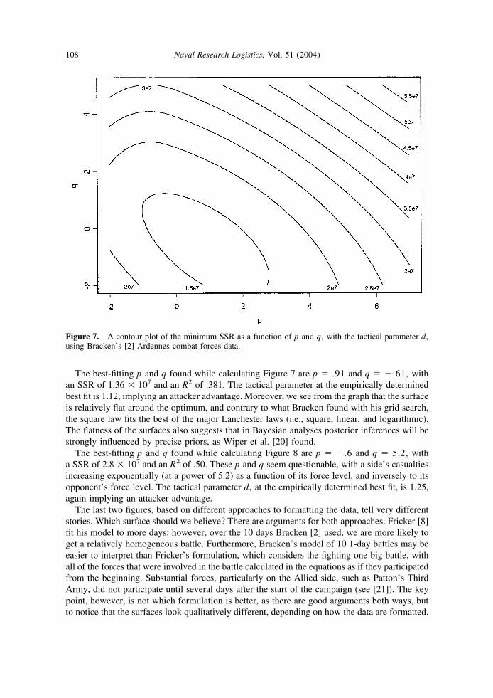
The best-fitting p and q found while calculating Figure 7 are p � .91 and q � �.61, withan SSR of 1.36 � 107 and an R2 of .381. The tactical parameter at the empirically determinedbest fit is 1.12, implying an attacker advantage. Moreover, we see from the graph that the surfaceis relatively flat around the optimum, and contrary to what Bracken found with his grid search,the square law fits the best of the major Lanchester laws (i.e., square, linear, and logarithmic).The flatness of the surfaces also suggests that in Bayesian analyses posterior inferences will bestrongly influenced by precise priors, as Wiper et al. [20] found.

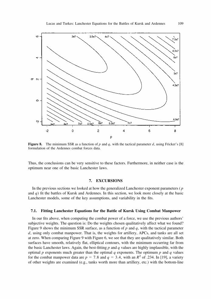
The best-fitting p and q found while calculating Figure 8 are p � �.6 and q � 5.2, witha SSR of 2.8 � 107 and an R2 of .50. These p and q seem questionable, with a side’s casualtiesincreasing exponentially (at a power of 5.2) as a function of its force level, and inversely to itsopponent’s force level. The tactical parameter d, at the empirically determined best fit, is 1.25,again implying an attacker advantage.

The last two figures, based on different approaches to formatting the data, tell very differentstories. Which surface should we believe? There are arguments for both approaches. Fricker [8]fit his model to more days; however, over the 10 days Bracken [2] used, we are more likely toget a relatively homogeneous battle. Furthermore, Bracken’s model of 10 1-day battles may beeasier to interpret than Fricker’s formulation, which considers the fighting one big battle, withall of the forces that were involved in the battle calculated in the equations as if they participatedfrom the beginning. Substantial forces, particularly on the Allied side, such as Patton’s ThirdArmy, did not participate until several days after the start of the campaign (see [21]). The keypoint, however, is not which formulation is better, as there are good arguments both ways, butto notice that the surfaces look qualitatively different, depending on how the data are formatted.

Figure 7. A contour plot of the minimum SSR as a function of p and q, with the tactical parameter d,using Bracken’s [2] Ardennes combat forces data.


Thus, the conclusions can be very sensitive to these factors. Furthermore, in neither case is theoptimum near one of the basic Lanchester laws.

7. EXCURSIONS

In the previous sections we looked at how the generalized Lanchester exponent parameters ( pand q) fit the battles of Kursk and Ardennes. In this section, we look more closely at the basicLanchester models, some of the key assumptions, and variability in the fits.

7.1. Fitting Lanchester Equations for the Battle of Kursk Using Combat Manpower

In our fits above, when computing the combat power of a force, we use the previous authors’subjective weights. The question is: Do the weights chosen qualitatively affect what we found?Figure 9 shows the minimum SSR surface, as a function of p and q, with the tactical parameterd, using only combat manpower. That is, the weights for artillery, APCs, and tanks are all setat zero. When comparing Figure 9 with Figure 6, we see that they are qualitatively similar. Bothsurfaces have smooth, relatively flat, elliptical contours, with the minimum occurring far fromthe basic Lanchester laws. Again, the best-fitting p and q values are highly implausible, with theoptimal p exponents much greater than the optimal q exponents. The optimum p and q valuesfor the combat manpower data are p � 7.8 and q � 3.4, with an R2 of .234. In [19], a varietyof other weights are examined (e.g., tanks worth more than artillery, etc.) with the bottom-line

Figure 8. The minimum SSR as a function of p and q, with the tactical parameter d, using Fricker’s [8]formulation of the Ardennes combat forces data.


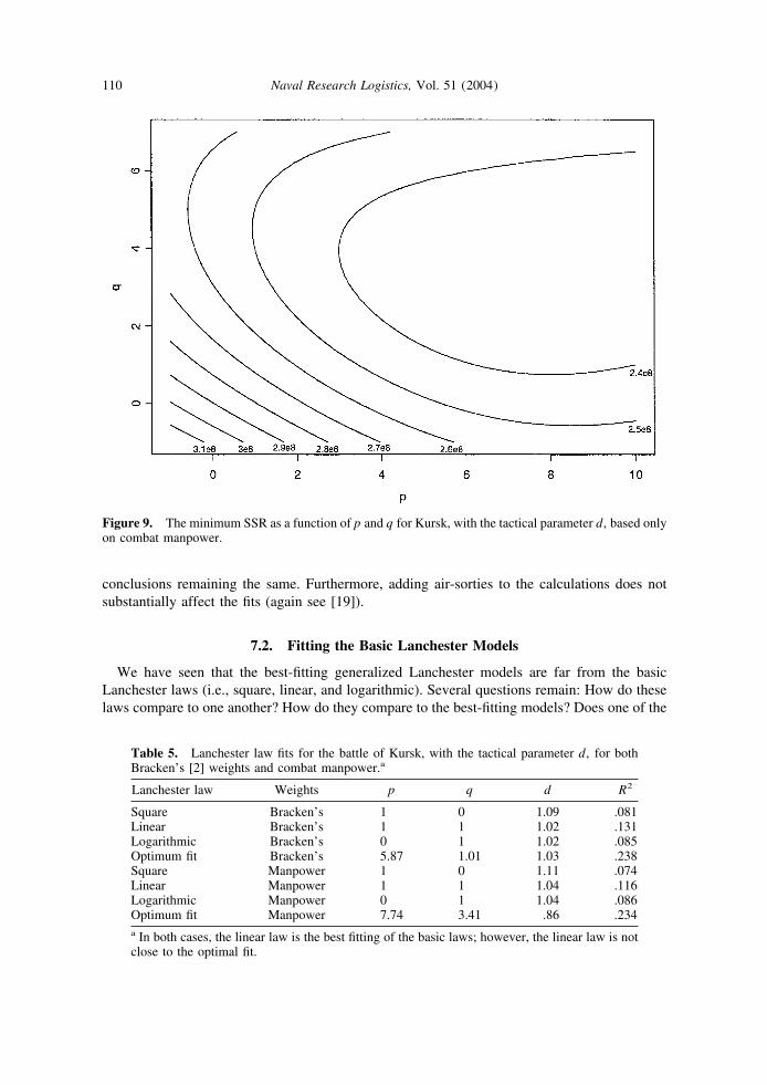
conclusions remaining the same. Furthermore, adding air-sorties to the calculations does notsubstantially affect the fits (again see [19]).

7.2. Fitting the Basic Lanchester Models

We have seen that the best-fitting generalized Lanchester models are far from the basicLanchester laws (i.e., square, linear, and logarithmic). Several questions remain: How do theselaws compare to one another? How do they compare to the best-fitting models? Does one of the

Table 5. Lanchester law fits for the battle of Kursk, with the tactical parameter d, for bothBracken’s [2] weights and combat manpower.a

Lanchester law Weights p q d R2

Square Bracken’s 1 0 1.09 .081Linear Bracken’s 1 1 1.02 .131Logarithmic Bracken’s 0 1 1.02 .085Optimum fit Bracken’s 5.87 1.01 1.03 .238Square Manpower 1 0 1.11 .074Linear Manpower 1 1 1.04 .116Logarithmic Manpower 0 1 1.04 .086Optimum fit Manpower 7.74 3.41 .86 .234a In both cases, the linear law is the best fitting of the basic laws; however, the linear law is notclose to the optimal fit.

Figure 9. The minimum SSR as a function of p and q for Kursk, with the tactical parameter d, based onlyon combat manpower.


basic laws consistently fit better across the breadth of models examined? This subsectionexamines these questions. Here, we consider only models with the tactical parameter d. Similarresults hold for models without d.

Table 5 shows how the basic Lanchester models (i.e., the square, linear, and logarithmic laws)fit the battle of Kursk using Bracken’s [2] weights (i.e., 1, 5, 20, and 40) and the manpower data.We see that, for both sets of weights, the linear law fits best among the basic laws, but it issignificantly inferior to the optimum fit, with an R2 of .131, compared to .238. While the linearlaw fits better than the square and logarithmic laws, its fit is not substantially better. Thus, thissuggests that with the right coefficients, any of the basic laws give about the same result. It isalso interesting to note that we get similar results using either weighting scheme, with Bracken’sweights generally fitting slightly better.

Table 6 displays similar information from the Ardennes campaign, using Bracken’s 10 daysof data [2]. There are several interesting features in the table. First, much better fits are achievedwith Bracken’s weights than with combat manpower. Furthermore, while the best-fitting basicLanchester law is the square law, with Bracken’s weights, all of the basic laws fit the data aboutas well. The R2 (.367) for the square law is only 3.6% below the optimum fit’s R2 (.381). It isinteresting to note that Bracken concluded that the best-fitting model was the linear law. Whythe discrepancy? Because Bracken used a grid search, which, as he noted in [2], by necessity,will not consider all of the parameter combinations for the various Lanchester laws. Whencomparing Tables 5 and 6, we see that the Ardennes data fit all of the models significantly betterthan the Kursk data when using Bracken’s weights. However, much of the difference is due tothe Soviet losses on 12 July, which is an outlier. Moreover, none of the basic laws stand out asthe best fitting.

7.3. Breaking the Battle of Kursk into Several Phases

An important assumption we (and the previous researchers) made when fitting the models isthat the attrition parameters (a and b) remain constant throughout the campaign. Surely, overthe course of the battle, the attrition rates waxed and waned to some extent. Ideally, we wouldestimate new coefficients for each day of the fighting, as the data are available daily. Unfortu-nately, if we do so, the system is overdetermined. That is, on each day, for any p and q, thereexist a and b such that the fitted casualties equal the real data.

To overcome this limitation, we break the battle into several phases, each of which is believedrelatively homogeneous. While several different partitions of the data were examined (see [19]),

Table 6. Lanchester law fits for the battle of the Ardennes using Bracken’s [2] combatmanpower model and the tactical parameter d.a

Lanchester law Weights p q d R2

Square Bracken’s 1 0 1.14 .367Linear Bracken’s 1 1 1.17 .291Logarithmic Bracken’s 0 1 1.23 .330Optimum fit Bracken’s .91 �.61 1.12 .381Square Manpower 1 0 1.04 .079Linear Manpower 1 1 1.06 �.226Logarithmic Manpower 0 1 1.10 .025Optimum fit Manpower .15 �.90 1.05 .280a Bracken’s weights provide much better fits than the manpower data. Also, the square law isthe best-fitting basic Lanchester law.


we focus here on what seems to be the most natural one based on the Kursk data and otherhistorical accounts. In our first phase—the first 2 days of the campaign—the Germans generallyattack prepared defenses. Our second phase contains days 3–7, which, by and large, had theGermans attacking hasty defenses. The 8th day of fighting, “the bloodbath at Prokorovka,” isunique and is considered a phase by itself. Of course, since this phase is only a single day, thereis a perfect fit (i.e., no residual error); thus, this removes the (outlying) eighth day from the fits.The fourth and last phase is days 9–14, in which the Soviets were more on the offensive, andthe battle intensity was fading, as can be seen in Figures 2, 4, and 5.

Table 7. Lanchester law fits for the battle of Kursk, using Bracken’s [2] weights,when the attrition coefficients are estimated in four separate phases.a

Lanchester law p q R2

Square 1 0 .804Linear 1 1 .816Logarithmic 0 1 .812Optimum fit 3.92 3.38 .832Four phase means fit Not applicable Not applicable .800a Almost all of the improvements in R2 are due to the differences in means betweenthe four phases.

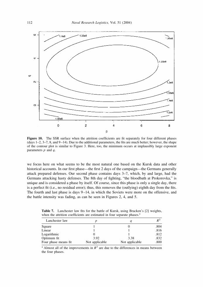
Figure 10. The SSR surface when the attrition coefficients are fit separately for four different phases(days 1–2, 3–7, 8, and 9–14). Due to the additional parameters, the fits are much better; however, the shapeof the contour plot is similar to Figure 3. Here, too, the minimum occurs at implausibly large exponentparameters p and q.


Fitting the model over multiple phases must result in a better overall fit because there areadditional parameters (degrees of freedom) to explain the variation in casualties. In our earlierfits there were five parameters ( p, q, a, b, and d). The new fits have 10 parameters: theexponent parameters p and q, and different attrition coefficients, a and b, in each of the fourphases. The defensive parameter d cannot be used here, because in each of the phases one sideis on the offensive throughout. Thus, within any phase, the effect of being on the defensive, asmeasured by d, is confounded with the phase’s attrition parameters.

The optimization routine, as before, searches for the p and q that minimize the sum of thesquared residuals between the fitted and actual casualties. For all p and q that are evaluated, ineach phase, the best-fitting a and b are determined by regression through the origin using thedata for that phase. This results in eight attrition coefficient parameters being calculated forevery p and q examined. For each p and q, the sum of the squared residuals (SSR) is calculatedby summing over the entire campaign (14 days) the squared difference between the fitted andactual casualties. Figure 10 displays the SSR surface as a function of p and q. This surface isstrikingly similar in shape to the surface in Figure 3, generated by the constant attritioncoefficient model, in that the contours are elliptic in shape, with the axes almost aligned to theordinate and the abscissa. In both figures, the ellipses are wider than they are tall, and theminimums are in the first quadrant at implausibly large exponent parameters. Some importantdifferences are: (1) the SSR surface for the four-phase model is much lower, i.e., a significantlybetter fit; and (2) the four-phase model surface is significantly flatter, implying that a widerrange of generalized Lanchester models are “near optimal.”

Table 7 displays the optimum and basic Lanchester model fits for the four-phase model. Theoptimum Lanchester exponent parameters for the four-phase model are p � 3.92 and q � 3.38,with an R2 of .832. This is a much better fit than any of the single-phase models we looked at.However, most of the improvement comes from partitioning the battle into the four phases. TheR2 that is obtained by using the mean loss in each phase, for each side, as the sides’ estimatedlosses, is .800. Consequently, the optimum four-phase Lanchester model, with 10 free param-eters, has an R2 of only .032 above the R2 obtained by using the four phase means. Thus,accounting for the varying intensity, terrains, postures, etc. explains significantly more of thevariation in losses than the Lanchester models do. This is consistent with what Hartley andHembold found in their study of the Inchon–Seoul battle [9]. Also, we can see from Table 7 thatthe basic Lanchester models fit only marginally better than the phase means, with the linear lawfitting slightly better than the square and logarithmic laws.

7.4. Assessing Differences in Fits

In the discussions above on the differences between various fits, as measured by R2, weloosely refer to some differences as significant and others as insignificant. In this section we usethe bootstrap (see Efron and Tibshirani [6]) to formally assess the differences in R2 betweenLanchester models. We focus on identifying differences that are of sufficient size that theordering of the estimates (different R2 values) is unlikely to be effected by the natural variationin the data. Keeping in mind that all battles are nonrepeatable events, we define the naturalvariation as the variation that would occur (due to the inherent randomness of combat) if manyessentially identical forces fought similar 14-day battles and the inevitable errors associated withrecording and collecting decades old combat data.

In fitting the Lanchester models above, the 14 days of the battle are essentially treated as 14minibattles. That is, for a given law (i.e., specific p and q), we find the values of a, b, and dwhich minimize R2 (or equivalently SSR) over the 14 days. Here, we quantify the variability in


R2, for each law, nonparametrically, by resampling the empirical daily attrition coefficients,from the 14 days, as follows. For each of the three basic Lanchester laws and the Lanchesteroptimum fit, using the law’s optimum d value, we calculate ai and bi for i � 1, 2, . . . , 14,where ai and bi are the daily attrition parameters that achieve equality in Eqs. (1) and (2). Thatis, the 14 (ai, bi) pairs are the attrition rates that actually occurred in the battle (according to thedata set) if the Lanchester law being used (to generate the resampled battles) held exactly. A“bootstrap battle” is created by sampling with replacement from the 14 (ai, bi) pairs andgenerating 14 daily “bootstrap casualties” by multiplying the 14 (ai, bi) pairs with the actualforce levels and the law’s optimum d (or 1/d, as appropriate). Thus, all of the bootstrap battleshave the same daily force levels, attacker, and defender as in the real battle. The bootstrap battlesare different from the real battle in that the daily casualties are generated as just specified.

Using the above procedure for the three basic Lanchester laws and the optimum Lanchesterfit, 1000 bootstrap battles (from the 1414 possible ones) are independently generated (sampled).In each of the 1000 bootstrap battles we find the best-fitting model (maximum R2) over a, b,and d, as before. This gives us a sample of 1000 bootstrap R2 values, which we label Ri

2, fori � 1, 2, . . . , 1,000. For each law, the Ri

2 values are sorted from smallest to largest. Theinterval from the 50th largest Ri

2 to the 950th largest Ri2 constitutes a 90% bootstrap percentile

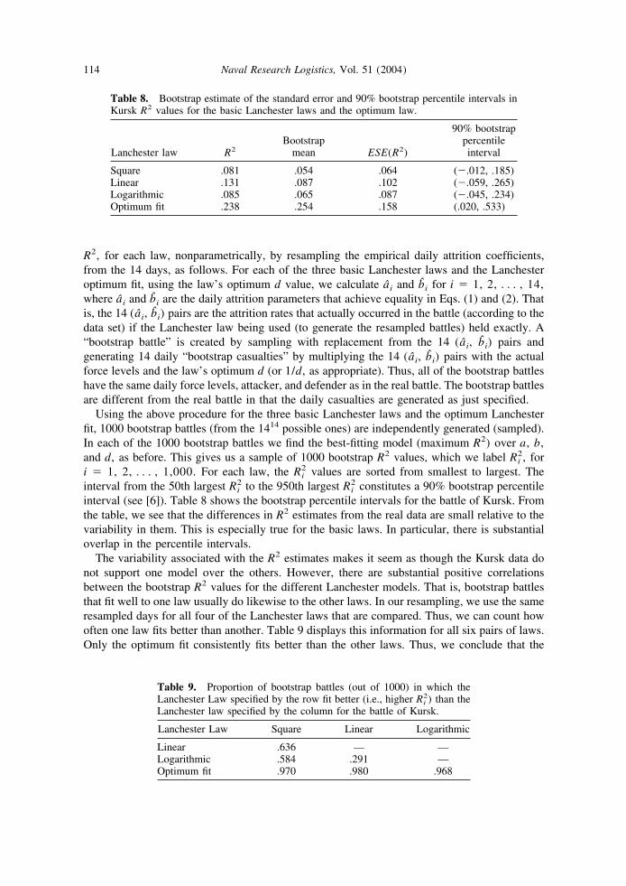
interval (see [6]). Table 8 shows the bootstrap percentile intervals for the battle of Kursk. Fromthe table, we see that the differences in R2 estimates from the real data are small relative to thevariability in them. This is especially true for the basic laws. In particular, there is substantialoverlap in the percentile intervals.

The variability associated with the R2 estimates makes it seem as though the Kursk data donot support one model over the others. However, there are substantial positive correlationsbetween the bootstrap R2 values for the different Lanchester models. That is, bootstrap battlesthat fit well to one law usually do likewise to the other laws. In our resampling, we use the sameresampled days for all four of the Lanchester laws that are compared. Thus, we can count howoften one law fits better than another. Table 9 displays this information for all six pairs of laws.Only the optimum fit consistently fits better than the other laws. Thus, we conclude that the

Table 8. Bootstrap estimate of the standard error and 90% bootstrap percentile intervals inKursk R2 values for the basic Lanchester laws and the optimum law.

Lanchester law R2Bootstrap

mean ESE(R2)

90% bootstrappercentileinterval

Square .081 .054 .064 (�.012, .185)Linear .131 .087 .102 (�.059, .265)Logarithmic .085 .065 .087 (�.045, .234)Optimum fit .238 .254 .158 (.020, .533)

Table 9. Proportion of bootstrap battles (out of 1000) in which theLanchester Law specified by the row fit better (i.e., higher Ri

2) than theLanchester law specified by the column for the battle of Kursk.

Lanchester Law Square Linear Logarithmic

Linear .636 — —Logarithmic .584 .291 —Optimum fit .970 .980 .968


natural variation in the data is such that for any given realization all of the basic Lanchester lawshad a reasonable chance (greater than a quarter of the time) of being a better fit than any otherbasic law.

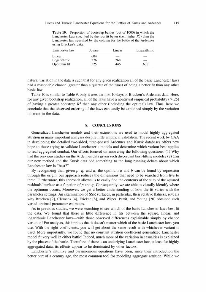
Table 10 is similar to Table 9, only it uses the first 10 days of Bracken’s Ardennes data. Here,for any given bootstrap realization, all of the laws have a nontrivial empirical probability (�.25)of having a greater bootstrap R2 than any other (including the optimal) law. Thus, here weconclude that the observed ordering of the laws can easily be explained simply by the variationinherent in the data.

8. CONCLUSIONS

Generalized Lanchester models and their extensions are used to model highly aggregatedattrition in many important analyses despite little empirical validation. The recent work by CAAin developing the detailed two-sided, time-phased Ardennes and Kursk databases offers newhope to those trying to validate Lanchester’s models and determine which variant best appliesto real aggregated combat. Our efforts focused on answering the following questions: (1) Whyhad the previous studies on the Ardennes data given such discordant best-fitting models? (2) Canour new method and the Kursk data add something to the long running debate about whichLanchester law is “best?”

By recognizing that, given p, q, and d, the optimum a and b can be found by regressionthrough the origin, our approach reduces the dimensions that need to be searched from five tothree. Furthermore, this approach allows us to easily find the contours of the sum of the squaredresiduals’ surface as a function of p and q. Consequently, we are able to visually identify wherethe optimum occurs. Moreover, we get a better understanding of how the fit varies with theparameter settings. An examination of SSR surfaces, in particular, their relative flatness, revealswhy Bracken [2], Clemens [4], Fricker [8], and Wiper, Pettit, and Young [20] obtained suchvaried optimal parameter estimates.

As in previous studies, we were searching to see which of the basic Lanchester laws best fitthe data. We found that there is little difference in fits between the square, linear, andlogarithmic Lanchester laws—with those observed differences explainable simply by chancevariation! For analysts, this implies that it doesn’t matter which of the basic Lanchester laws youuse. With the right coefficients, you will get about the same result with whichever variant isused. More importantly, we found that no constant attrition coefficient generalized Lanchestermodel fit very well in either battle! Indeed, much more of the variation in casualties is explainedby the phases of the battle. Therefore, if there is an underlying Lanchester law, at least for highlyaggregated data, its effects appear to be dominated by other factors.

Lanchester’s intuitive and parsimonious equations have been, since their introduction thebetter part of a century ago, the most common tool for modeling aggregate attrition. While we

Table 10. Proportion of bootstrap battles (out of 1000) in which theLanchester Law specified by the row fit better (i.e., higher Ri

2) than theLanchester law specified by the column for the battle of the Ardennesusing Bracken’s data.

Lanchester law Square Linear Logarithmic

Linear .604 — —Logarithmic .376 .268 —Optimum fit .525 .446 .638


are wary about making too much from two battles (though these are all we have of this type),this research adds to the evidence that Lanchester equations may be too blunt of an instrumentfor modeling the attrition of highly aggregated forces. Indeed, it is asking a lot to address mostof the complexities of combat attrition in a model with only a handful (four or five in this paper)of parameters. The failure to find any good-fitting Lanchester model suggests that it may bebeneficial to look for new approaches to model highly aggregated attrition.

ACKNOWLEDGMENTS

This work was inspired and shaped by the efforts of Jerry Bracken and Ron Fricker, to whomthanks are given. The authors are also grateful to E. B. Vandiver III and his staff at the Centerfor Army Analysis, who provided the data and excellent feedback. Finally, the reviews providedby the associate editor and a referee significantly improved the content and clarity of this paper.

REFERENCES

[1] J. Appleget, “The combat simulation of Desert Storm with applications for contingency operations,”Warfare modeling, J. Bracken, M. Kress, and R. Rosenthal (Editors), Military Operations ResearchSociety, Alexandria, VA, 1995, pp. 549–571.

[2] J. Bracken, Lanchester models of the Ardennes Campaign, Naval Res Logist 42 (1995), 559–577.[3] Center for Army Analysis, Kursk operation simulation and validation exercise—Phase II (KOSAVE

II), The U.S. Army’s Center for Strategy and Force Evaluation Study Report, CAA-SR-98-7, FortBelvoir, VA, September 1998.

[4] S. Clemens, The application of Lanchester Models to the Battle of Kursk, unpublished manuscript,Yale University, New Haven, CT, 5 May 1997.

[5] Data Memory Systems Inc., The Ardennes Campaign simulation Data base (ACSDB) Final Report,Center for Army Analysis, Fort Belvoir, VA, February 1990.

[6] B. Efron and R. Tibshirani, An introduction to the bootstrap, Chapman and Hall, New York, 1993.[7] J. Engel, Verification of Lanchester’s Law, Oper Res 2 (1954), 163–171.[8] R. Fricker, Attrition models of the Ardennes Campaign, Naval Res Logist 45 (1998), 1–22.[9] D. Hartley III and R. Helmbold, Validating Lanchester’s Square Law and other attrition models,

Naval Res Logist 42 (1995), 609–633.[10] D. Glantz and J. House, The Battle of Kursk (Modern War Studies), University Press of Kansas,

Lawrence, KS, 1999.[11] F. Lanchester, Aircraft in warfare: The dawn of the fourth arm, Constable, London, 1916.[12] R. Myers, Classical and modern regression with applications, Duxbury, Boston, 1986.[13] J. Neter, M. Kutner, C. Nachtsheim, and W. Wasserman, Applied linear statistical models, 3rd

edition, Irwin, Chicago, IL, 1996.[14] M. Osipov, The influence of the numerical strength of engaged sides on their casualties, Voenniy Sb

(Military Coll) (6–10) (1915).[15] R. Peterson, On the “Logarithmic Law” of combat and its application to tank combat, Oper Res 15

(1967), 557–558.[16] R. Speight, Lanchester’s equations and the structure of the operational campaign: Within-campaign

effects, Mil Oper Res 6(1) (2001), 81–103.[17] J. Taylor, Lanchester Models of warfare (two volumes), Operations Research Society of America,

Arlington, VA, 1983.[18] P. Tsouras, The Great Patriotic War, Presidio Press, Novato, CA, 1992.[19] T. Turkes, Fitting Lanchester and other equations to the Battle of Kursk data, Masters Thesis,

Department of Operations Research, Naval Postgraduate School, Monterey, CA, March 2000.[20] M. Wiper, L. Pettit, and K. Young, Bayesian inference for a Lanchester type combat model, Naval

Res Logist 47 (2000), 541–558.[21] P. Young (Editor), Great generals and their battles, The Military Press, Greenwich, CT, 1984.[22] http://dspace.dial.pipex.com/town/avenue/vy75/, last accessed 15 January 2003.


Documents

2004 Fitting Lanchester Equations to the Battles of Kursk ... · 2004 Fitting Lanchester Equations to the ... Fitting Lanchester Equations to the Battles of Kursk and Ardennes