Embed Size (px)
Citation preview

2003-11-06Dan Ellis 1
ELEN E4810: Digital Signal Processing
Topic 8: Filter Design: IIR
1. Filter Design Specifications
2. Analog Filter Design
3. Digital Filters from Analog Prototypes
2003-11-06Dan Ellis 2
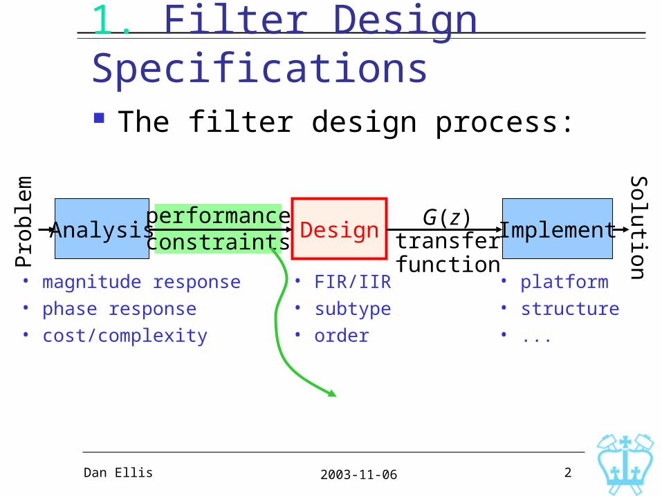
1. Filter Design Specifications The filter design process:
Design ImplementAnalysis
Pro
blem
Solution
G(z)transferfunction
performanceconstraints
• magnitude response• phase response• cost/complexity
• FIR/IIR• subtype• order
• platform• structure• ...
2003-11-06Dan Ellis 3
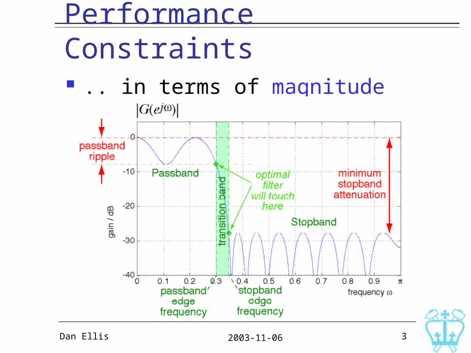
Performance Constraints .. in terms of magnitude response:
2003-11-06Dan Ellis 4
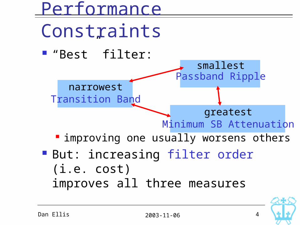
“Best” filter:
improving one usually worsens others But: increasing filter order (i.e. cost)
improves all three measures
Performance Constraints
smallestPassband Ripple
greatestMinimum SB Attenuation
narrowestTransition Band

2003-11-06Dan Ellis 5
Passband Ripple
Assume peak passband gain = 1then minimum passband gain =
Or, ripple
€
1
1+ε 2
€
αmax = 20 log10 1+ε 2 dB
PB rippleparameter

2003-11-06Dan Ellis 6
Stopband Ripple
Peak passband gain is A larger than peak stopband gain
Hence, minimum stopband attenuation
SB rippleparameter
€
α s = −20 log101A = 20 log10 A dB

2003-11-06Dan Ellis 7
Filter Type Choice: FIR vs. IIRFIR
No feedback(just zeros)
Always stable Can be
linear phase
High order (20-2000)
Unrelated to continuous-time filtering
IIR Feedback
(poles & zeros) May be unstable Difficult to control
phase
Typ. < 1/10th order of FIR (4-20)
Derive from analog prototype
BUT
2003-11-06Dan Ellis 8
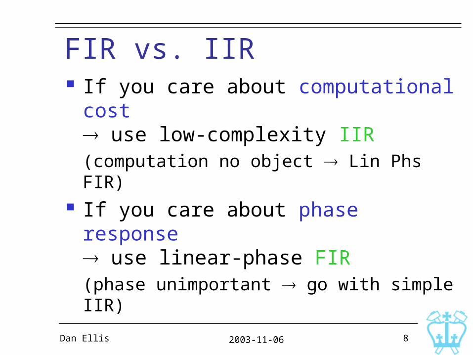
FIR vs. IIR If you care about computational cost use low-complexity IIR(computation no object Lin Phs FIR)
If you care about phase response use linear-phase FIR(phase unimportant go with simple IIR)

2003-11-06Dan Ellis 9
IIR Filter Design IIR filters are directly related to
analog filters (continuous time) via a mapping of H(s) (CT) to H(z) (DT) that
preserves many properties Analog filter design is sophisticated
signal processing research since 1940s
Design IIR filters via analog prototype hence, need to learn some CT filter design
2003-11-06Dan Ellis 10
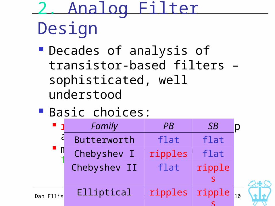
2. Analog Filter Design Decades of analysis of transistor-based
filters – sophisticated, well understood Basic choices:
ripples vs. flatness in stop and/or passband more ripples narrower transition band
Family PB SB
Butterworth flat flat
Chebyshev I ripples flat
Chebyshev II flat ripples
Elliptical ripples ripples
2003-11-06Dan Ellis 11
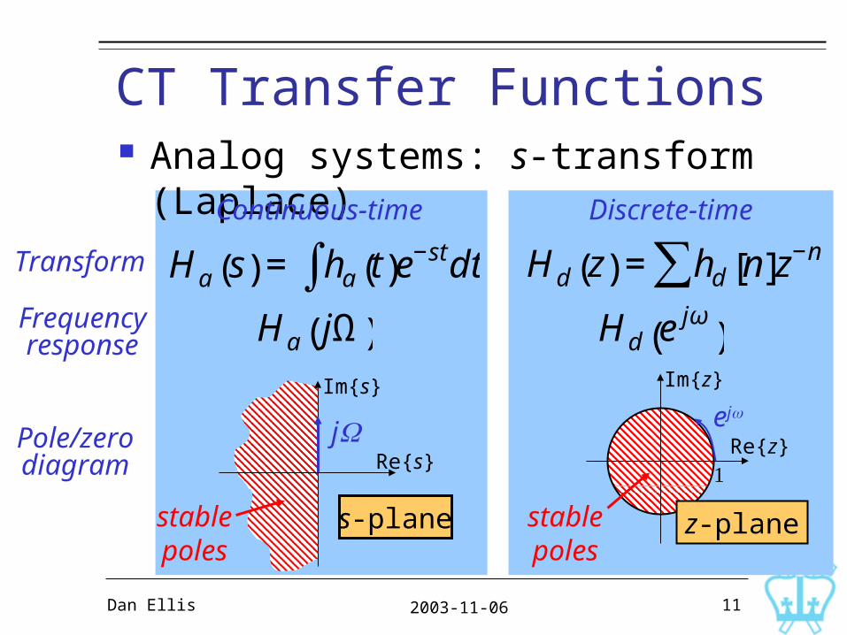
CT Transfer Functions Analog systems: s-transform (Laplace)
Continuous-time Discrete-time
€
Ha s( ) = ha t( )e−stdt∫
€
Hd z( ) = hd n[ ]z−n∑Transform
Frequencyresponse
Pole/zerodiagram
€
Ha jΩ( )
€
Hd e jω( )
s-plane
Re{s}
Im{s}
j
stablepoles
stablepoles
z-plane
Re{z}
Im{z}
ej
2003-11-06Dan Ellis 12
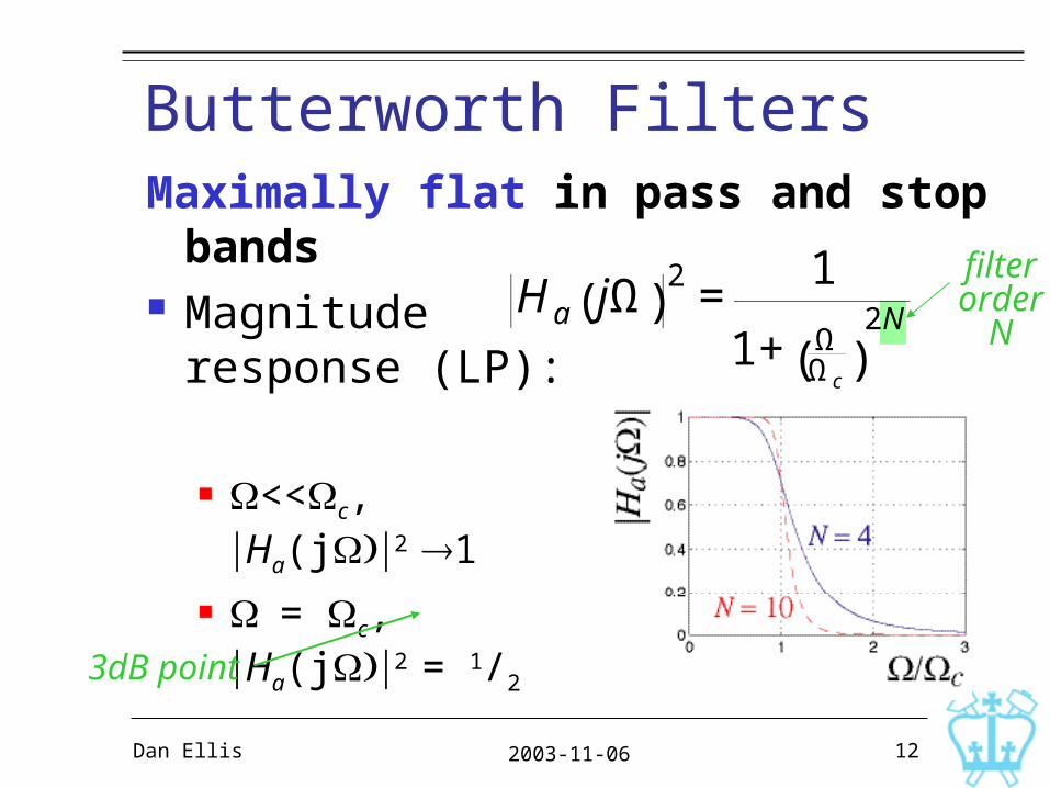
Maximally flat in pass and stop bands Magnitude
response (LP):
<<c, Ha(j2 1
= c, Ha(j2 = 1/2
Butterworth Filters
€
Ha jΩ( )2
=1
1+ ΩΩc
( )2N
filterorder
N
3dB point
2003-11-06Dan Ellis 13
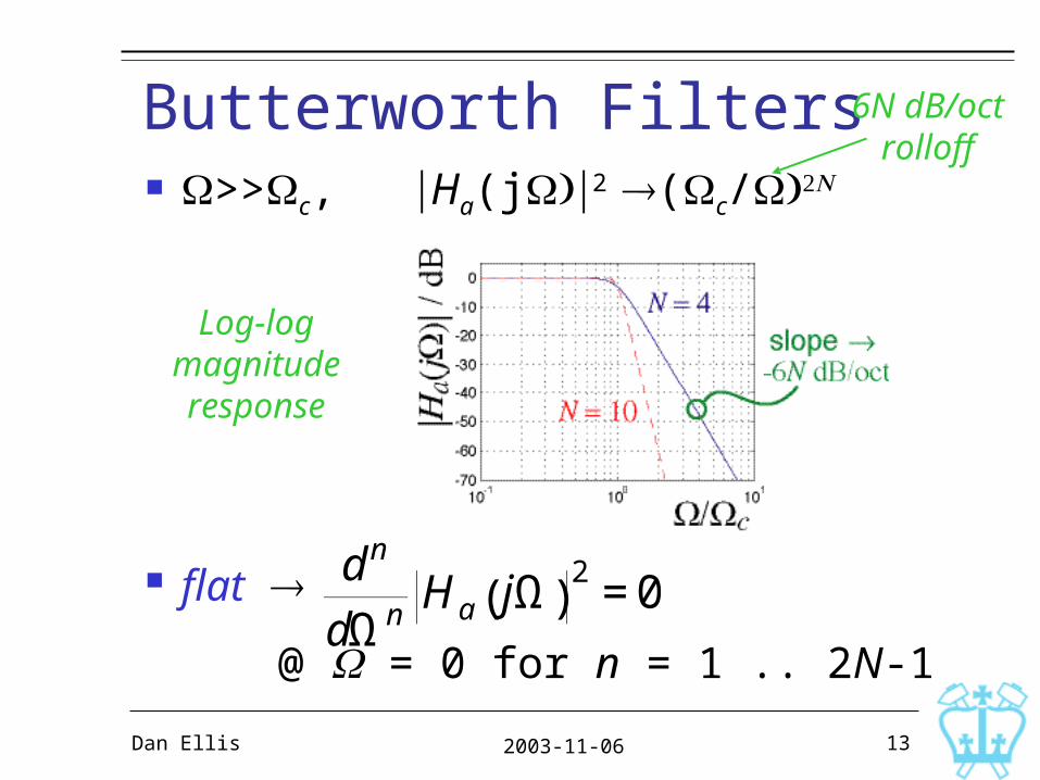
Butterworth Filters >>c, Ha(j2 (c/
flat
@ = 0 for n = 1 .. 2N-1
€
d n
dΩnHa jΩ( )
2= 0
Log-logmagnituderesponse
6N dB/octrolloff

2003-11-06Dan Ellis 14
Butterworth Filters How to meet design specifications?
€
1
1+Ω p
Ωc( )
2N=
1
1+ε 2
€
1
1+Ω p
Ωc( )
2N=
1
A2
€
N ≥12
log10A 2−1ε 2( )
log10Ωs
Ω p( )
DesignEquation
€
k1 =ε
A2 −1=“discrimination”, <<1
€
k =Ω p
Ωs=“selectivity”, < 1
2003-11-06Dan Ellis 15
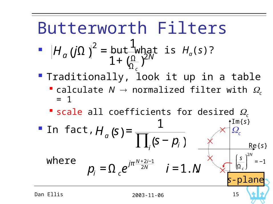
Butterworth Filters but what is Ha(s)?
Traditionally, look it up in a table calculate N normalized filter with c = 1 scale all coefficients for desired c
In fact,
where
€
Ha jΩ( )2
=1
1+ ( ΩΩc
)2N
€
Ha s( ) =1s − pi( )
i∏
€
pi = Ωcejπ N +2 i−1
2N i =1..Ns-plane
Re{s}
Im{s}c
€
sΩc
⎛
⎝ ⎜
⎞
⎠ ⎟
2N
= −1
2003-11-06Dan Ellis 16
Butterworth Example
€
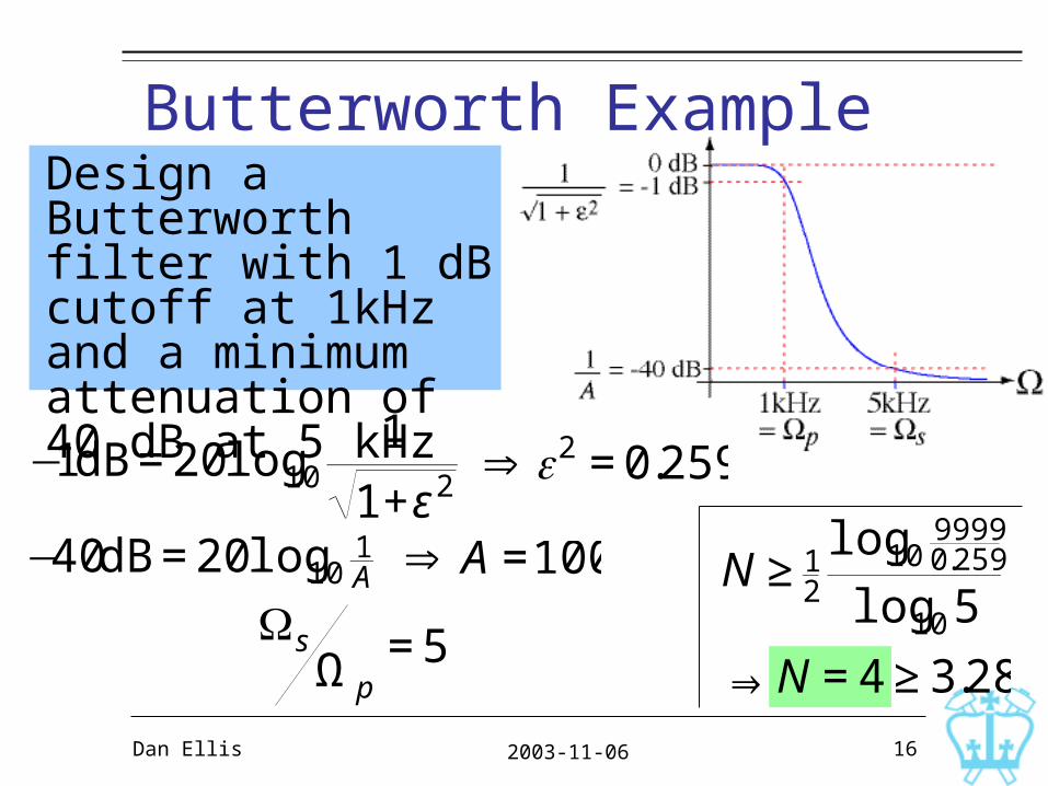
−1dB = 20 log101
1+ε 2
€
⇒ ε2 = 0.259
€
−40dB = 20 log101A
€
⇒ A =100
Design a Butterworth filter with 1 dB cutoff at 1kHz and a minimum attenuation of 40 dB at 5 kHz
€
sΩ p
= 5
€
N ≥ 12
log1099990.259
log10 5
⇒ N = 4 ≥ 3.28
2003-11-06Dan Ellis 17
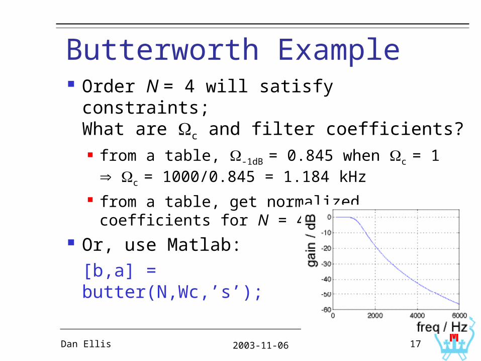
Butterworth Example Order N = 4 will satisfy constraints;
What are c and filter coefficients? from a table, -1dB = 0.845 when c = 1 c = 1000/0.845 = 1.184 kHz
from a table, get normalized coefficients for N = 4, scale by 1184
Or, use Matlab:
[b,a] = butter(N,Wc,’s’);
M

2003-11-06Dan Ellis 18
Chebyshev I Filter Equiripple in passband (flat in stopband) minimize maximum error
€
Ha jΩ( )2
=1
1+ε 2TN2 ( Ω
Ω p)
€
TN Ω( ) =cos N cos−1 Ω( ) Ω ≤1
cosh N cosh−1 Ω( ) Ω >1
⎧ ⎨ ⎪
⎩ ⎪
Chebyshevpolynomialof order N
2003-11-06Dan Ellis 19
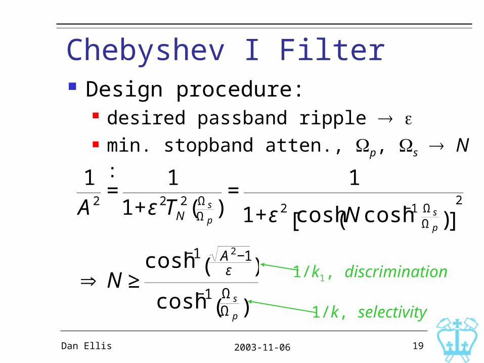
Chebyshev I Filter Design procedure:
desired passband ripple ε min. stopband atten., p, s N :
€
1A2
=1
1+ε 2TN2 (Ωs
Ω p)
=1
1+ε 2 cosh N cosh−1 ΩsΩ p( )[ ]
2
€
⇒ N ≥cosh−1 A 2−1
ε( )
cosh−1 Ωs
Ω p( )
1/k1, discrimination
1/k, selectivity
2003-11-06Dan Ellis 20
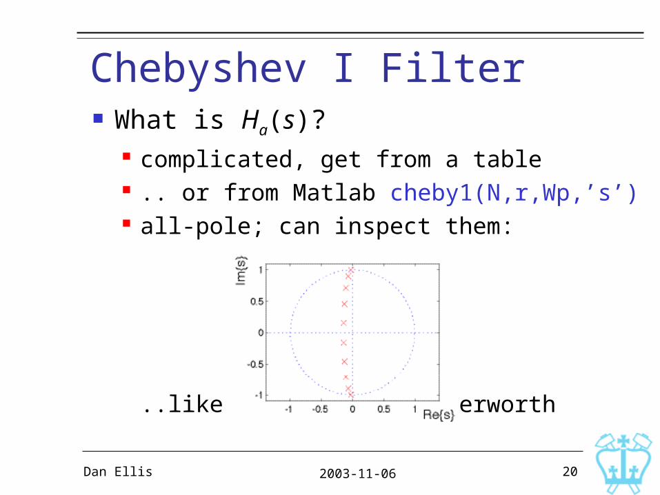
Chebyshev I Filter What is Ha(s)?
complicated, get from a table .. or from Matlab cheby1(N,r,Wp,’s’) all-pole; can inspect them:
..like squashed-in Butterworth

2003-11-06Dan Ellis 21
Chebyshev II Filter Flat in passband, equiripple in stopband
Filter has poles and zeros (some ) Complicated pole/zero pattern€
Ha jΩ( )2
=1
1+ε 2TN (Ωs
Ω p)
TN (Ωs
Ω )
⎛
⎝ ⎜ ⎜
⎞
⎠ ⎟ ⎟
2
zeros on imaginary axis
constant
~1/TN(1/)
2003-11-06Dan Ellis 22
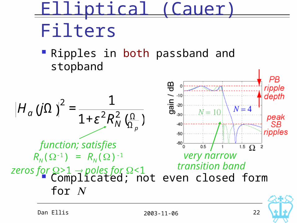
Elliptical (Cauer) Filters Ripples in both passband and stopband
Complicated; not even closed form for
very narrow transition band
€
Ha jΩ( )2
=1
1+ε 2 RN2 ( Ω
Ω p)
function; satisfiesRN(-1) = RN()-1
zeros for >1 poles for <1
2003-11-06Dan Ellis 23
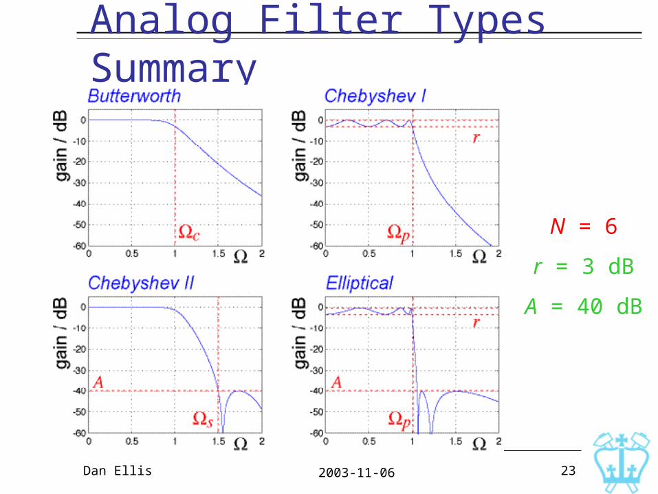
Analog Filter Types Summary
N = 6
r = 3 dB
A = 40 dB
2003-11-06Dan Ellis 24
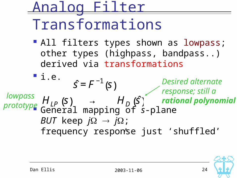
Analog Filter Transformations All filters types shown as lowpass;
other types (highpass, bandpass..)derived via transformations
i.e.
General mapping of s-planeBUT keep j j ; frequency response just ‘shuffled’
€
HLP s( )
ˆ s = F −1 s( )
→ HD ˆ s ( )
Desired alternateresponse; still arational polynomial
lowpassprototype
^
2003-11-06Dan Ellis 25
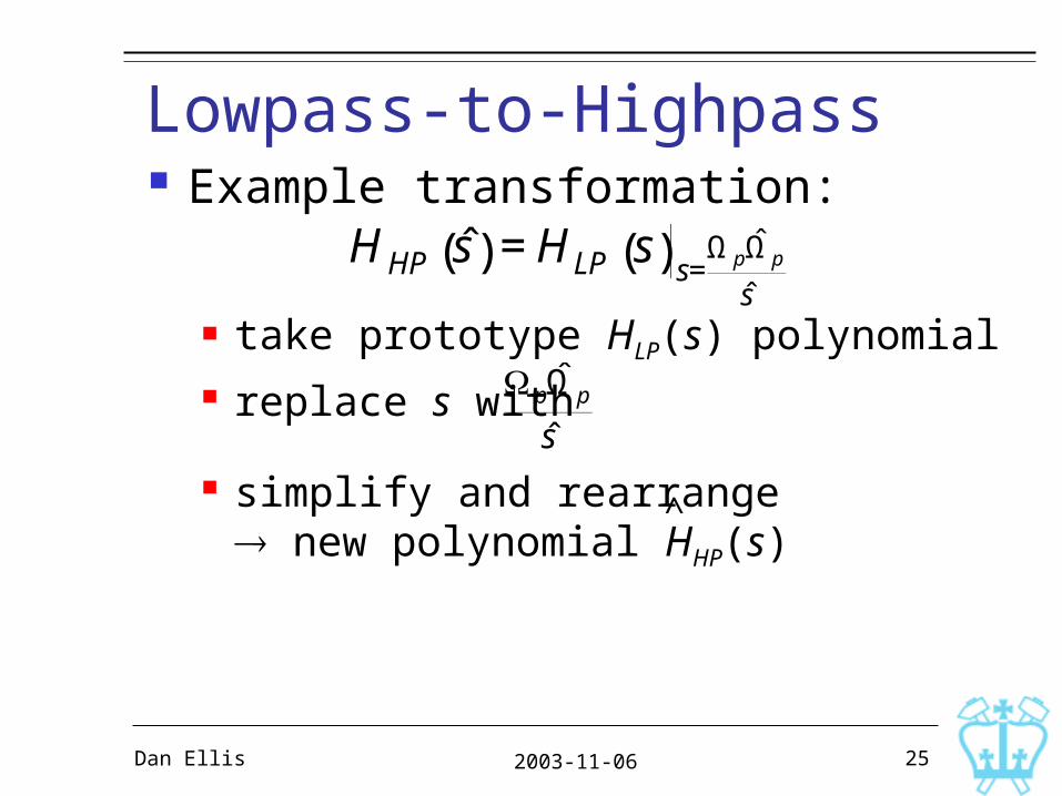
Lowpass-to-Highpass Example transformation:
take prototype HLP(s) polynomial replace s with
simplify and rearrange new polynomial HHP(s)
€
H HP ˆ s ( ) = HLP s( ) s=Ω p
ˆ Ω pˆ s
€
pˆ Ω p
ˆ s
^
2003-11-06Dan Ellis 26
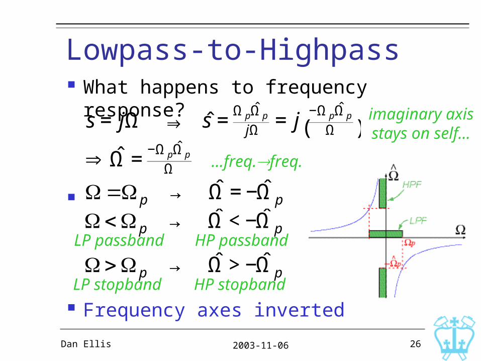
Lowpass-to-Highpass What happens to frequency response?
Frequency axes inverted
€
s = jΩ ⇒ ˆ s =Ω p
ˆ Ω pjΩ = j
−Ω pˆ Ω p
Ω( )
€
⇒ ˆ Ω =−Ω p
ˆ Ω pΩ
€
= p → ˆ Ω = − ˆ Ω p
€
< p → ˆ Ω < − ˆ Ω pLP passband HP passband
€
> p → ˆ Ω > − ˆ Ω pLP stopband HP stopband
imaginary axisstays on self...
...freq.freq.
2003-11-06Dan Ellis 27
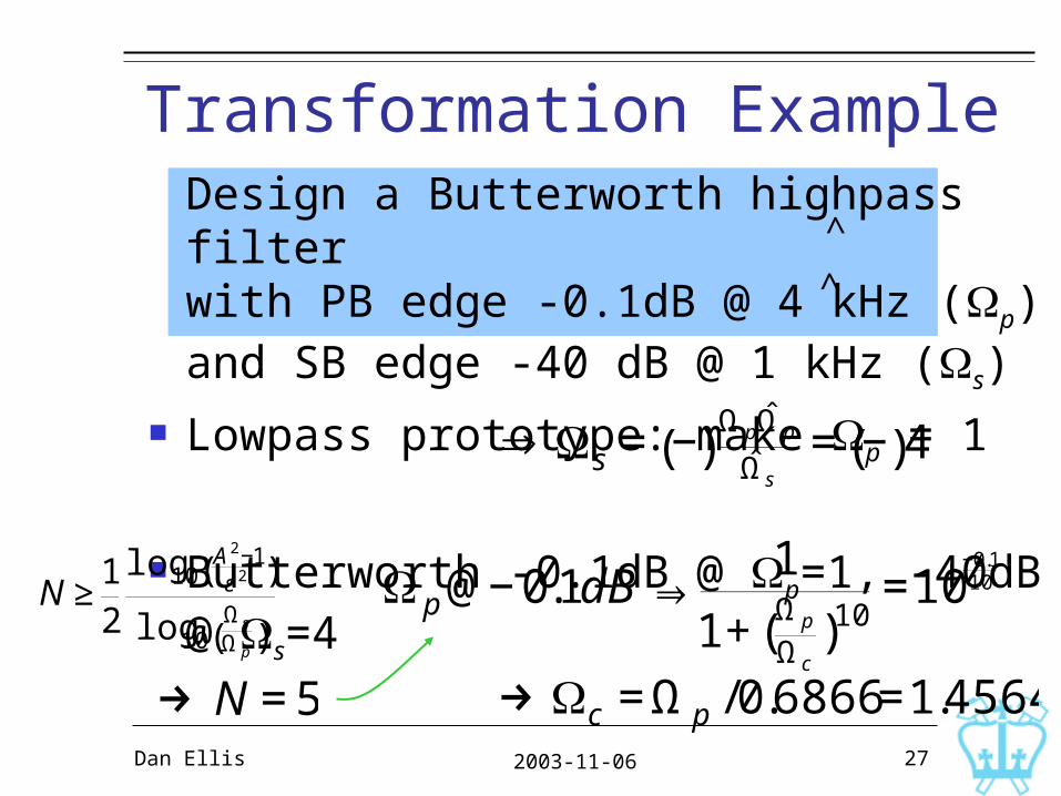
Transformation ExampleDesign a Butterworth highpass filter with PB edge -0.1dB @ 4 kHz ( p)and SB edge -40 dB @ 1 kHz ( s)
Lowpass prototype: make p = 1
Butterworth -0.1dB @ p=1, -40dB @ s=4
^
^
€
⇒ s = −( )Ω p
ˆ Ω pˆ Ω s
= −( )4
€
N ≥12
log10A 2−1ε 2( )
log10Ωs
Ω p( )
€
→ N = 5
€
p @− 0.1dB ⇒1
1+ (Ω p
Ωc)10
=10−0.110
€
→ c = Ω p /0.6866 =1.4564

2003-11-06Dan Ellis 28
Transformation Example LPF proto has
Map to HPF:
€
pl = Ωcejπ N +2l −1
2N Re{s}
Im{s}c
€
⇒ HLP s( ) =Ωc
N
s − pil( )i=1
N
∏
€
H HP ˆ s ( ) = HLP s( ) s=Ω p
ˆ Ω pˆ s
€
⇒ H HP ˆ s ( ) =Ωc
N
Ω pˆ Ω p
ˆ s − pl( )l =1
N∏
=Ωc
N ˆ s N
Ω pˆ Ω p − pl ˆ s ( )l =1
N∏
N zeros@ s = 0^
new poles @ s = pp/pl^ ^
2003-11-06Dan Ellis 29
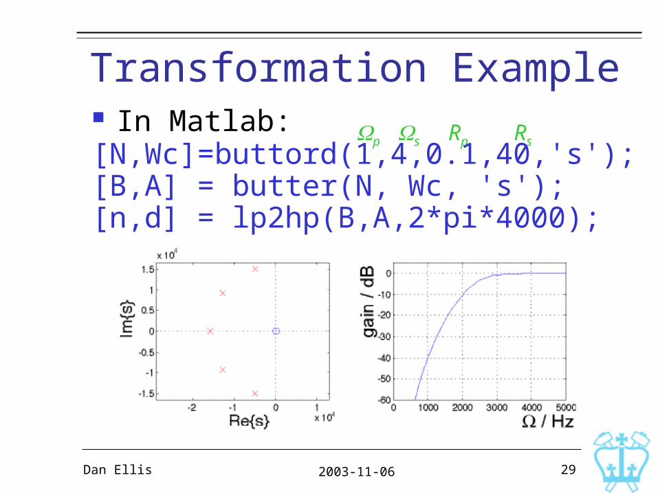
Transformation Example In Matlab:[N,Wc]=buttord(1,4,0.1,40,'s');[B,A] = butter(N, Wc, 's');[n,d] = lp2hp(B,A,2*pi*4000);
p s Rp Rs
2003-11-06Dan Ellis 30
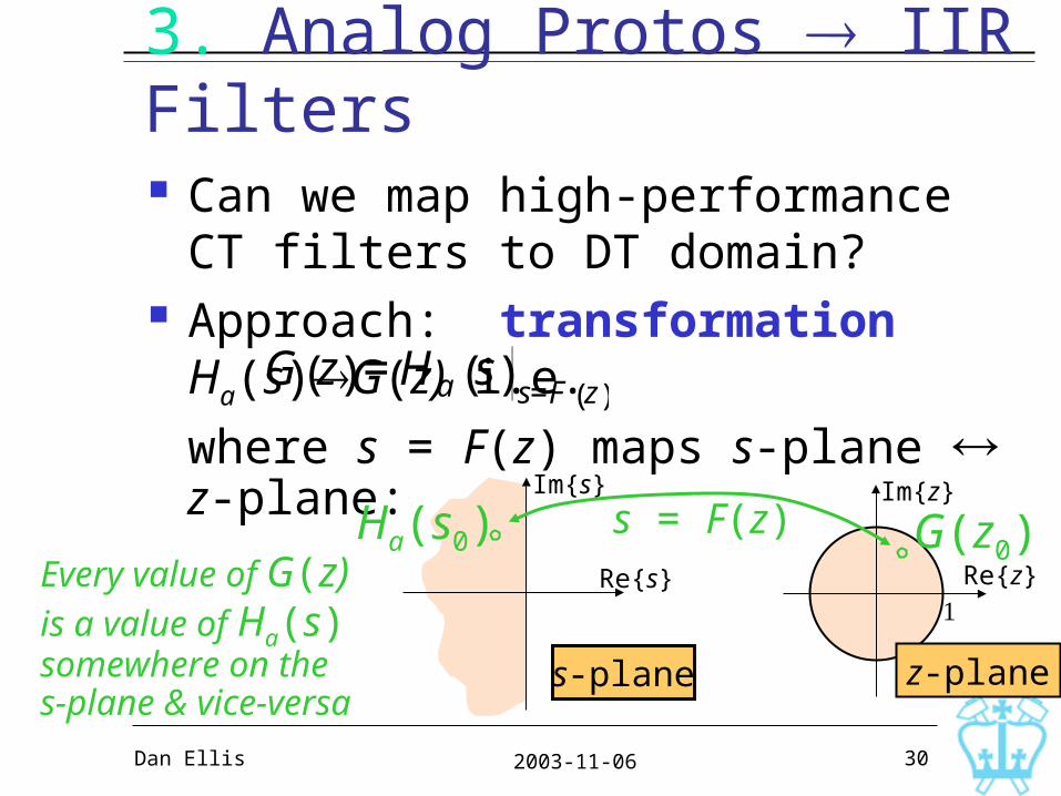
3. Analog Protos IIR Filters Can we map high-performance CT
filters to DT domain? Approach: transformation Ha(s) G(z)
i.e. where s = F(z) maps s-plane z-plane:
€
G z( ) = Ha s( ) s=F z( )
s-plane
Re{s}
Im{s}
z-plane
Re{z}
Im{z}
Ha(s0) G(z0)Every value of G(z)is a value of Ha(s)somewhere on the s-plane & vice-versa
s = F(z)

2003-11-06Dan Ellis 31
CT to DT Transformation Desired properties for s = F(z):
s-plane j axis z-plane unit circle preserves frequency response values
s-plane LHHP z-plane unit circle interior preserves stability of poles
s-plane
Re{s}
Im{s}
j
z-plane
Re{z}
Im{z}
ej
LHHPUCI
Imu.c.
2003-11-06Dan Ellis 32
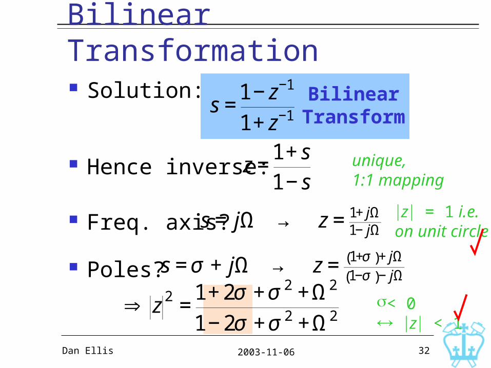
Bilinear Transformation Solution:
Hence inverse:
Freq. axis?
Poles?
€
s =1 − z−1
1+ z−1
BilinearTransform
€
z =1+ s1− s
unique, 1:1 mapping
€
s = jΩ → z = 1+ jΩ1− jΩ
z = 1 i.e.on unit circle
€
s = σ + jΩ → z = 1+σ( )+ jΩ1−σ( )− jΩ
€
⇒ z 2 =1+ 2σ +σ 2 +Ω2
1− 2σ +σ 2 +Ω2< 0 z < 1
2003-11-06Dan Ellis 33
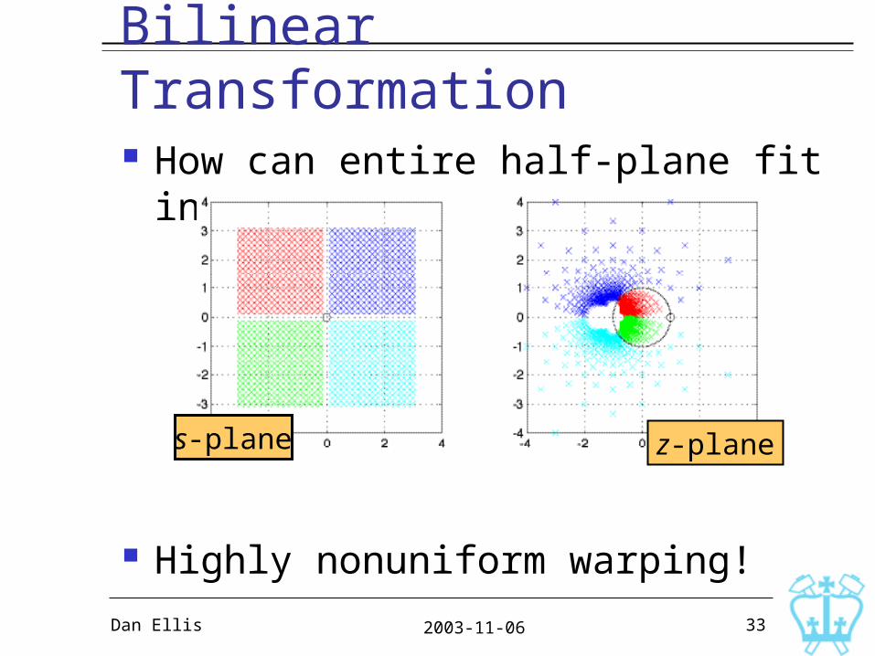
Bilinear Transformation How can entire half-plane fit inside u.c.?
Highly nonuniform warping!
s-plane z-plane
2003-11-06Dan Ellis 34
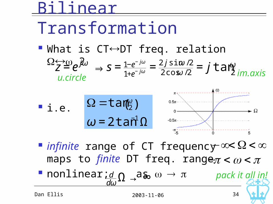
Bilinear Transformation What is CTDT freq. relation ?
i.e.
infinite range of CT frequency maps to finite DT freq. range
nonlinear; as
€
z = e jω ⇒ s = 1−e− jω
1+e− jω = 2 j sinω /22 cosω /2 = j tan ω
2u.circle im.axis
€
=tan ω2( )
ω = 2 tan−1 Ω
€
−∞<<∞
€
− < <
€
ddω Ω → ∞ pack it all in!
2003-11-06Dan Ellis 35
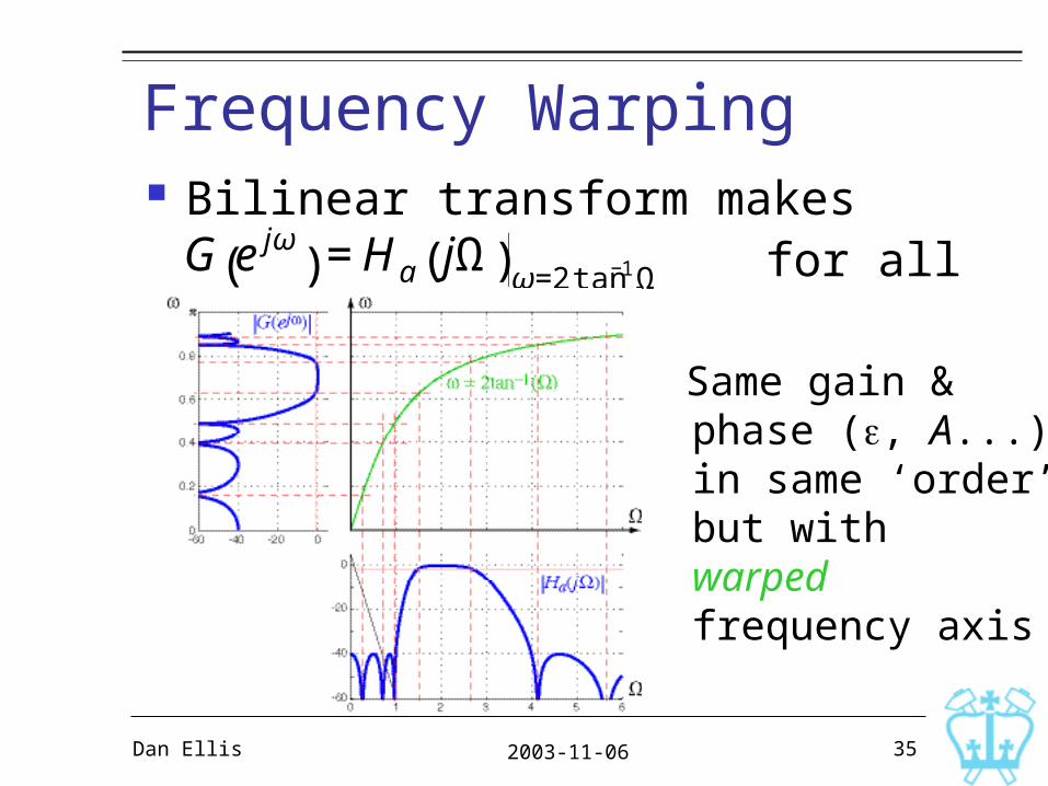
Frequency Warping Bilinear transform makes
for all
€
G e jω( ) = Ha jΩ( )ω=2 tan−1 Ω
Same gain & phase (ε, A...), in same ‘order’, but with warped frequency axis

2003-11-06Dan Ellis 36
Design Procedure Obtain DT filter specs:
general form (LP, HP...), ‘Warp’ frequencies to CT:
Design analog filter for
Ha(s), CT filter polynomial
Convert to DT domain: G(z), rational polynomial in z
Implement digital filter!
€
p ,ωs,1
1+ε 2 , 1A
€
p = tanω p
2
€
s = tan ωs
2
€
p ,Ωs,1
1+ε 2 , 1A
€
G z( ) = Ha s( ) s=1−z−1
1+z−1
Old-style
2003-11-06Dan Ellis 37
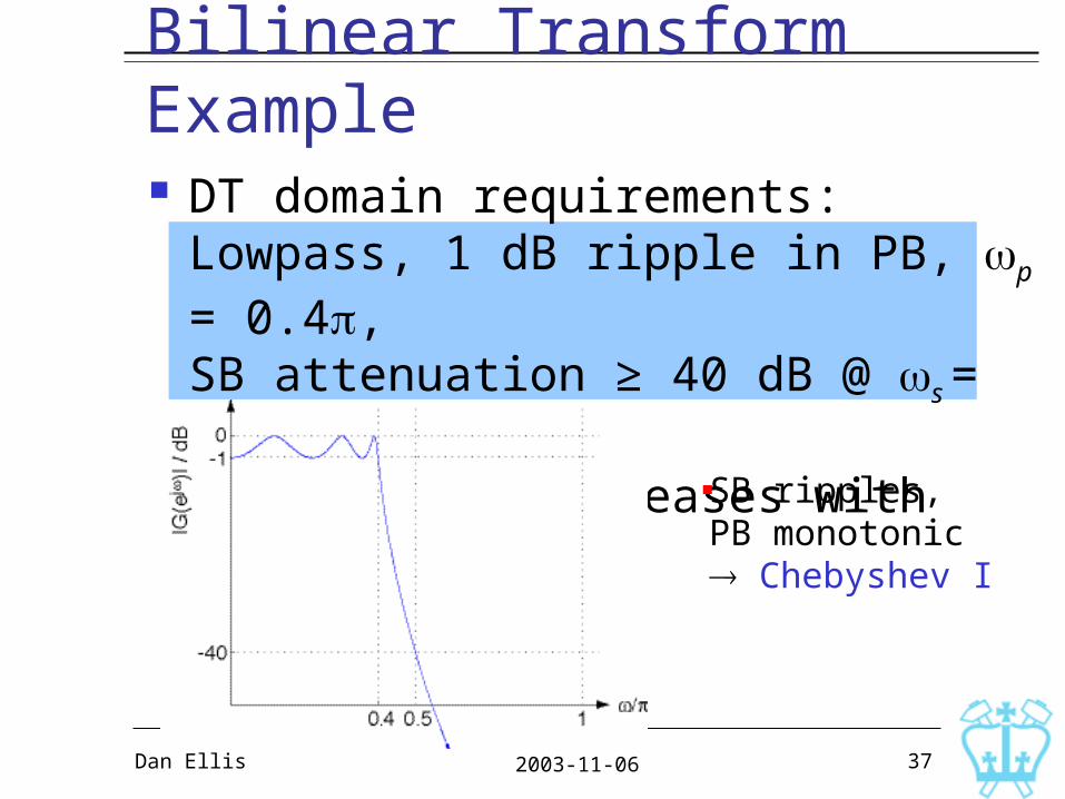
Bilinear Transform Example DT domain requirements:
Lowpass, 1 dB ripple in PB, p = 0.4 ,SB attenuation ≥ 40 dB @ s = 0.5 ,attenuation increases with frequency
SB ripples,PB monotonic Chebyshev I

2003-11-06Dan Ellis 38
Bilinear Transform Example Warp to CT domain:
Magnitude specs:1 dB PB ripple
40 dB SB atten.
€
p = tanω p
2 = tan 0.2π = 0.7265 rad/sec
€
s = tan ωs
2 = tan 0.25π =1.0 rad/sec
€
⇒ 11+ε 2 =10−1/20 = 0.8913⇒ ε = 0.5087
€
⇒ 1A =10−40 /20 = 0.01⇒ A =100
2003-11-06Dan Ellis 39
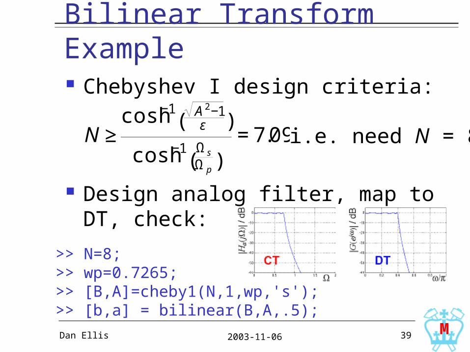
Bilinear Transform Example Chebyshev I design criteria:
Design analog filter, map to DT, check:
€
N ≥cosh−1 A 2−1
ε( )
cosh−1 Ωs
Ω p( )
= 7.09 i.e. need N = 8
>> N=8;>> wp=0.7265;>> [B,A]=cheby1(N,1,wp,'s');>> [b,a] = bilinear(B,A,.5);
M
2003-11-06Dan Ellis 40
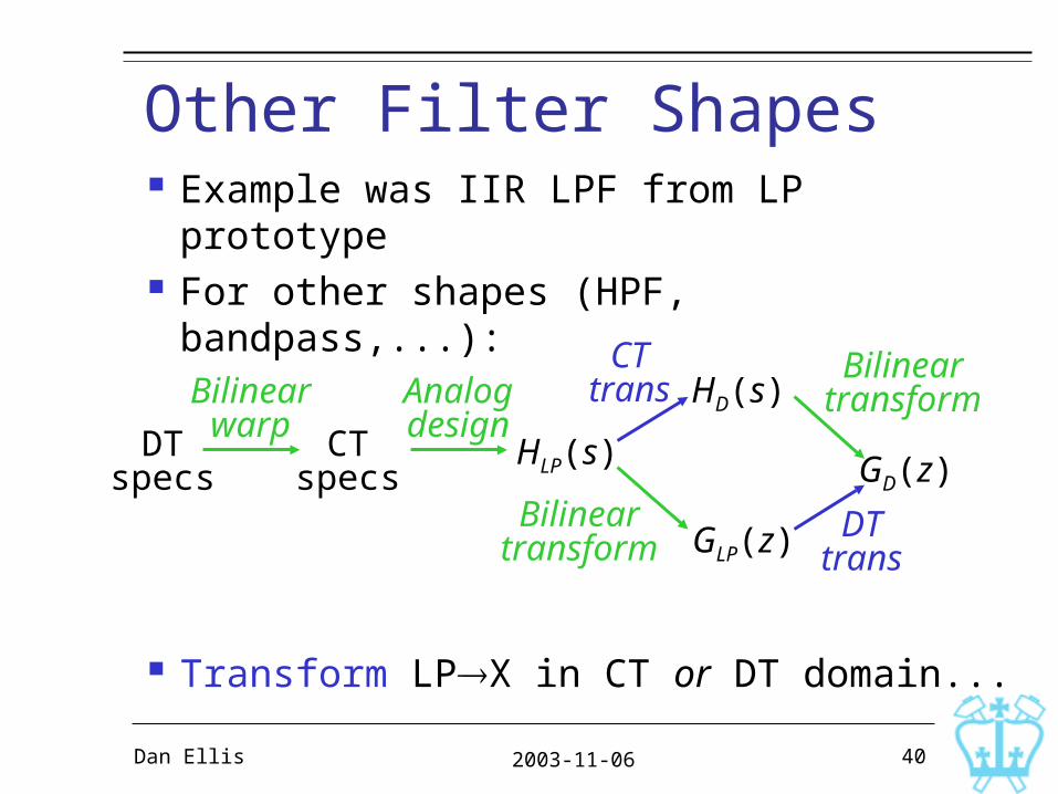
Other Filter Shapes Example was IIR LPF from LP prototype For other shapes (HPF, bandpass,...):
Transform LP X in CT or DT domain...
DTspecs
CTspecs
HLP(s)
HD(s)
GLP(z)
GD(z)
Bilinearwarp
Analogdesign
CTtrans
DTtrans
Bilineartransform
Bilineartransform
2003-11-06Dan Ellis 41
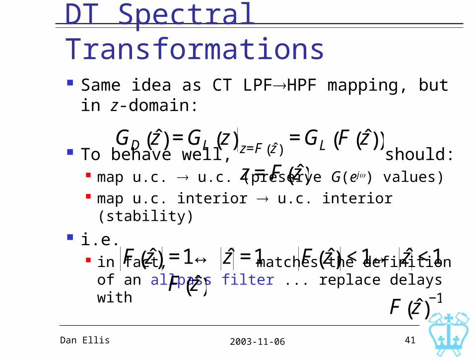
DT Spectral Transformations Same idea as CT LPF HPF mapping,
but in z-domain:
To behave well, should: map u.c. u.c. (preserve G(ej) values) map u.c. interior u.c. interior (stability)
i.e. in fact, matches the definition of an
allpass filter ... replace delays with
€
z = F ˆ z ( )
€
GD ˆ z ( ) = GL z( ) z=F ˆ z ( )= GL F ˆ z ( )( )
€
F ˆ z ( ) =1↔ ˆ z =1
€
F ˆ z ( ) <1↔ ˆ z <1
€
F ˆ z ( )
€
F ˆ z ( )−1

2003-11-06Dan Ellis 42
DT Frequency Warping Simplest mapping
has effect of warping frequency axis:
€
z = F ˆ z ( ) = ˆ z −α1−α ˆ z
€
ˆ z = e j ˆ ω ⇒ z = e jω =e j ˆ ω −α
1 − ae j ˆ ω
€
⇒ tan ω2( ) = 1+α
1−α tan ˆ ω 2( )
α > 0 :expand HF
α < 0 :expand LF
2003-11-06Dan Ellis 43
Another Design Example Spec:
Bandpass, from 800-1600 Hz (SR = 8kHz) Ripple = 1dB, min. stopband atten. = 60 dB 8th order, best transition band
Use elliptical for best performance Full design path:
design analog LPF prototype analog LPF BPF CT BPF DT BPF (Bilinear)

2003-11-06Dan Ellis 44
Another Design Example Or, do it all in one step in Matlab:
[b,a] = ellip(8,1,60, [800
1600]/(8000/2));