Embed Size (px)
Citation preview
8/20/2019 2 Random Numbers (1)
http://slidepdf.com/reader/full/2-random-numbers-1 1/47
© Kleber Barcia V.
Chapter 2
Random Numbers
1. Random-number generation
2. Random-variable generation

8/20/2019 2 Random Numbers (1)
http://slidepdf.com/reader/full/2-random-numbers-1 2/47
© Kleber Barcia V.
Chapter 2
2
1. Objectives. Random numbers
Discuss how the random numbers are
generated.
Introduce the subsequent testing for
randomness:
Frequency test
Autocorrelation test.
8/20/2019 2 Random Numbers (1)
http://slidepdf.com/reader/full/2-random-numbers-1 3/47
© Kleber Barcia V.
Chapter 2
3
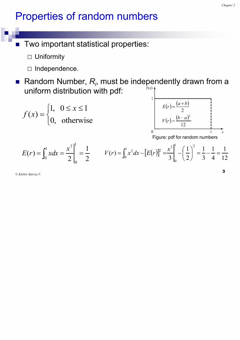
Properties of random numbers
Two important statistical properties:
Uniformity
Independence.
Random Number, R i , must be independently drawn from auniform distribution with pdf:
Figure: pdf for random numbers
2
1
2)(
1
0
21
0
x xdxr E
12
1
4
1
3
1
2
1
3)(
21
0
31
0
22
xr E dx xr V
12
22
abr V
bar E
otherwise ,0
10 ,1)(
x x f

8/20/2019 2 Random Numbers (1)
http://slidepdf.com/reader/full/2-random-numbers-1 4/47
© Kleber Barcia V.
Chapter 2
4
Generation of pseudo-random numbers
“Pseudo”, because generating numbers using a known
method removes the potential for true randomness.
Goal: To produce a sequence of numbers in [0,1] that
simulates, or imitates, the ideal properties of random numbers
(RN).
Important considerations in RN routines:
Fast
Portable to different computers
Have sufficiently long cycle
Replicable
Closely approximate the ideal statistical properties of uniformity
and independence.
8/20/2019 2 Random Numbers (1)
http://slidepdf.com/reader/full/2-random-numbers-1 5/47
© Kleber Barcia V.
Chapter 2
5
Techniques to generate random numbers
Middle-square algorithm
Middle-product algorithm
Constant multiplier algorithm
Linear algorithm
Multiplicative congruential algorithm
Additive congruential algorithm
Congruential non-linear algorithms
Quadratic
Blumy Shub

8/20/2019 2 Random Numbers (1)
http://slidepdf.com/reader/full/2-random-numbers-1 6/47
© Kleber Barcia V.
Chapter 2
6
Middle-square algorithm
1. Select a seed x0 with D digits (D > 3)
2. Rises to the square: (x0)2
3. Takes the four digits of the Center = x1
4. Rises to the square: (x1)2
5. Takes the four digits of the Center = x2
6. And so on. Then convert these values to r 1 between
0 and 1
If it is not possible to obtain the D digits in the Center,
add zeros to the left.
8/20/2019 2 Random Numbers (1)
http://slidepdf.com/reader/full/2-random-numbers-1 7/47© Kleber Barcia V.
Chapter 2
7
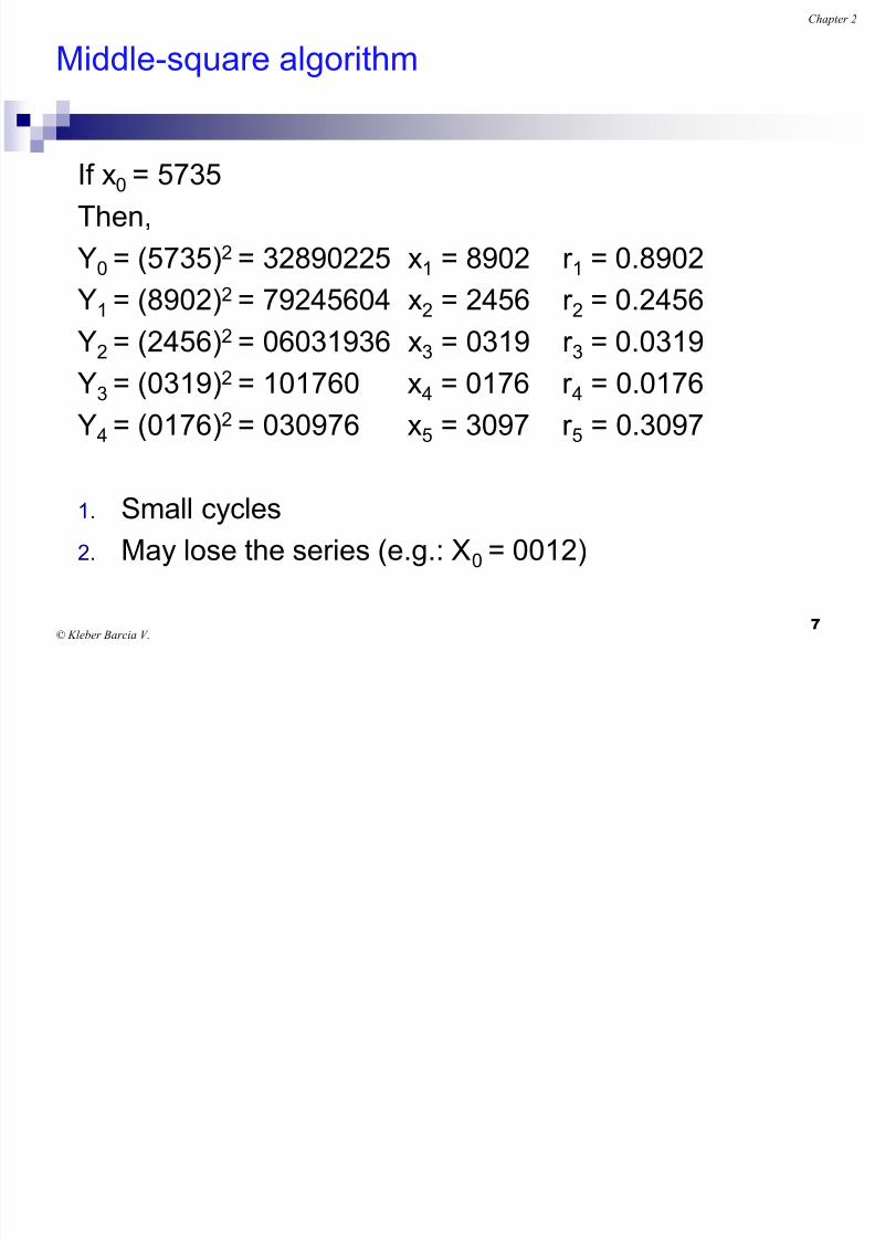
Middle-square algorithm
If x0 = 5735
Then,
Y0 = (5735)2 = 32890225 x1 = 8902 r 1 = 0.8902
Y1 = (8902)2
= 79245604 x2 = 2456 r 2 = 0.2456Y2 = (2456)2 = 06031936 x3 = 0319 r 3 = 0.0319
Y3 = (0319)2 = 101760 x4 = 0176 r 4 = 0.0176
Y4 = (0176)2 = 030976 x5 = 3097 r 5 = 0.3097
1. Small cycles
2. May lose the series (e.g.: X0 = 0012)

8/20/2019 2 Random Numbers (1)
http://slidepdf.com/reader/full/2-random-numbers-1 8/47© Kleber Barcia V.
Chapter 2
8
Middle-product algorithm
It requires 2 seeds of D digits
1. Select 2 seeds x0 and x1 with D > 3
2. Y0 = x0* x1 xi = digits of the center3. Yi = x1*xi xi+1 = digits of the center
If it is not possible to obtain the D digits in the center, add
zeros to the left.
8/20/2019 2 Random Numbers (1)
http://slidepdf.com/reader/full/2-random-numbers-1 9/47© Kleber Barcia V.
Chapter 2
9
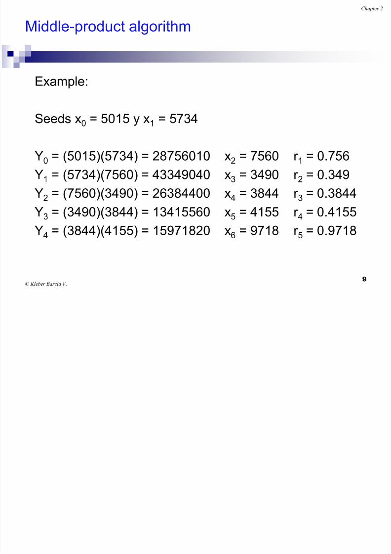
Middle-product algorithm
Example:
Seeds x0 = 5015 y x1 = 5734
Y0 = (5015)(5734) = 28756010 x2 = 7560 r 1 = 0.756
Y1 = (5734)(7560) = 43349040 x3 = 3490 r 2 = 0.349
Y2 = (7560)(3490) = 26384400 x4 = 3844 r 3 = 0.3844
Y3 = (3490)(3844) = 13415560 x5 = 4155 r 4 = 0.4155
Y4 = (3844)(4155) = 15971820 x6 = 9718 r 5 = 0.9718
8/20/2019 2 Random Numbers (1)
http://slidepdf.com/reader/full/2-random-numbers-1 10/47© Kleber Barcia V.
Chapter 2
10
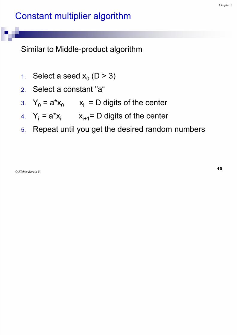
Constant multiplier algorithm
Similar to Middle-product algorithm
1. Select a seed x0 (D > 3)
2. Select a constant "a“
3. Y0 = a*x0 xi = D digits of the center
4. Yi = a*xi xi+1= D digits of the center
5. Repeat until you get the desired random numbers

8/20/2019 2 Random Numbers (1)
http://slidepdf.com/reader/full/2-random-numbers-1 11/47© Kleber Barcia V.
Chapter 2
11
Constant multiplier algorithm
Example:
If: seed x0 = 9803 and constant a = 6965
Y0 = (6965)(9803) = 68277895 x1 = 2778 r 1 = 0.2778
Y1 = (6965)(2778) = 19348770 x2 = 3487 r 2 = 0.3487
Y2 = (6965)(3487) = 24286955 x3 = 2869 r 3 = 0.2869
Y3 = (6965)(2869) = 19982585 x4 = 9825 r 4 = 0.9825
Y4 = (6965)(9825) = 68431125 x5 = 4311 r 5 = 0.4311
8/20/2019 2 Random Numbers (1)
http://slidepdf.com/reader/full/2-random-numbers-1 12/47© Kleber Barcia V.
Chapter 2
12
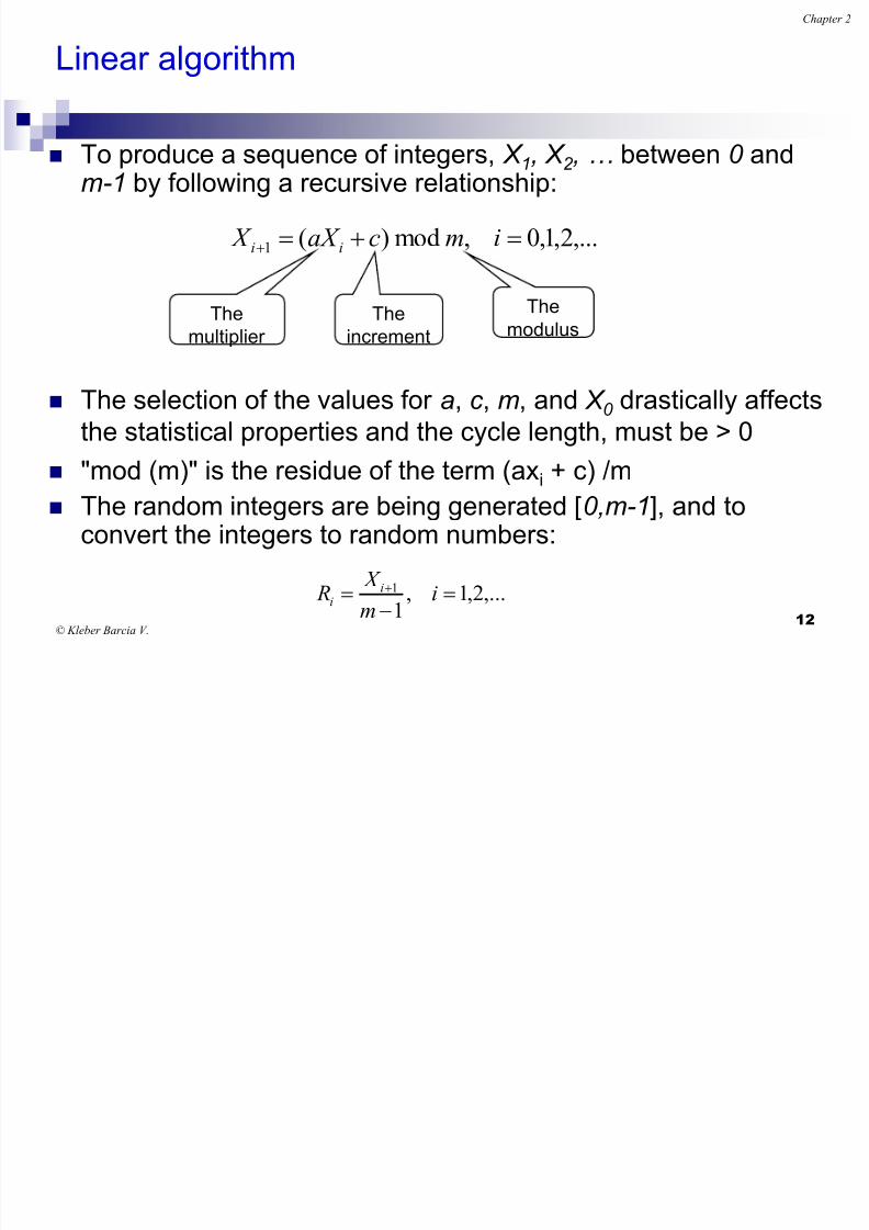
Linear algorithm
To produce a sequence of integers, X 1, X 2 , … between 0 andm-1 by following a recursive relationship:
The selection of the values for a, c , m, and X 0 drastically affects
the statistical properties and the cycle length, must be > 0
"mod (m)" is the residue of the term (axi + c) /m
The random integers are being generated [0,m-1], and toconvert the integers to random numbers:
,...2,1,0 ,mod)(1 imcaX X ii
The
multiplier
The
increment
Themodulus
,...2,1 ,1
1
im
X R i
i

8/20/2019 2 Random Numbers (1)
http://slidepdf.com/reader/full/2-random-numbers-1 13/47© Kleber Barcia V.
Chapter 2
13
Linear algorithm
Example:
Use X 0 = 27 , a = 17 , c = 43 y m = 100
The values of x i and r i are:
X 1 = (17*27+43) mod 100 = 502 mod 100 = 2 r 1 = 2/99 = 0.02
X 2 = (17*2+43) mod 100 = 77 mod 100 = 77 r 2 = 77/99 = 0.77
X 3 = (17*77+43) mod 100 = 1352 mod,100 = 52 r 3 = 52/99 = 0.52
The maximum life period N is equal to m
8/20/2019 2 Random Numbers (1)
http://slidepdf.com/reader/full/2-random-numbers-1 14/47© Kleber Barcia V.
Chapter 2
14
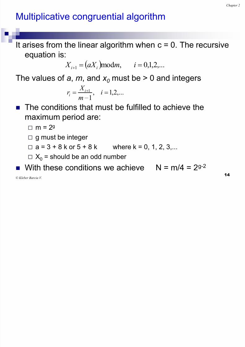
Multiplicative congruential algorithm
It arises from the linear algorithm when c = 0. The recursiveequation is:
The values of a, m, and x 0 must be > 0 and integers
The conditions that must be fulfilled to achieve the
maximum period are:
m = 2g
g must be integer
a = 3 + 8 k or 5 + 8 k where k = 0, 1, 2, 3,...
X0 = should be an odd number
With these conditions we achieve N = m/4 = 2
g-2
,...2,1,0 ,mod1 imaX X ii
,...2,1 ,1
1
im
X r ii
8/20/2019 2 Random Numbers (1)
http://slidepdf.com/reader/full/2-random-numbers-1 15/47© Kleber Barcia V.
Chapter 2
15
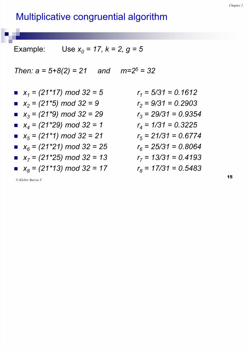
Multiplicative congruential algorithm
Example: Use x 0 = 17 , k = 2 , g = 5
Then: a = 5+8(2) = 21 and m=2 5 = 32
x 1 = (21*17) mod 32 = 5 r 1 = 5/31 = 0.1612
x 2 = (21*5) mod 32 = 9 r 2 = 9/31 = 0.2903
x 3 = (21*9) mod 32 = 29 r 3 = 29/31 = 0.9354
x 4
= (21*29) mod 32 = 1 r 4
= 1/31 = 0.3225
x 5 = (21*1) mod 32 = 21 r 5 = 21/31 = 0.6774
x 6 = (21*21) mod 32 = 25 r 6 = 25/31 = 0.8064
x 7 = (21*25) mod 32 = 13 r 7 = 13/31 = 0.4193
x 8
= (21*13) mod 32 = 17 r 8
= 17/31 = 0.5483

8/20/2019 2 Random Numbers (1)
http://slidepdf.com/reader/full/2-random-numbers-1 16/47
© Kleber Barcia V.
Chapter 2
16
Additive congruential algorithm
Requires a sequence of n integer numbers x1, x2, x3,…xn
to generate new random numbers starting at xn+1, xn+2,…
The recursive equation is:
1m
X r ii
N nnim x x x niii ,...,2,1 ,mod1

8/20/2019 2 Random Numbers (1)
http://slidepdf.com/reader/full/2-random-numbers-1 17/47
© Kleber Barcia V.
Chapter 2
17
Additive congruential algorithm
Example:
x1 =65, x2 = 89, x3 = 98, x4 = 03, x5 = 69, m = 100
x 6 =(x 5 +x 1 )mod100 = (69+65)mod100 = 34 r 6 = 34/99 = 0.3434
x 7 =(x 6 +x 2 )mod100 = (34+89)mod100 = 23 r 7 = 23/99 = 0.2323
x 8 =(x 7 +x 3 )mod100 = (23+98)mod100 = 21 r 8 = 21/99 = 0.2121
x 9=(x 8 +x 4 )mod100 = (21+03)mod100 = 24 r 9= 24/99 = 0.2424
x 10 =(x 9+x 5 )mod100 = (24+69)mod100 = 93 r 10 = 93/99 = 0.9393
x 11=(x 10 +x 6 )mod100 = (93+34)mod100 = 27 r 11= 27/99 = 0.2727
x 12 =(x 11+x 7 )mod100 = (27+23)mod100 = 50 r 12 = 50/99 = 0.5050

8/20/2019 2 Random Numbers (1)
http://slidepdf.com/reader/full/2-random-numbers-1 18/47
© Kleber Barcia V.
Chapter 2
18
Congruential non-linear algorithms
Quadratic:
Conditions to achieve a maximum period N = m
m = 2g
g must be integer
a must be an even number
c must be an odd number(b-a)mod4 = 1
1
1
m
X r ii
N imcbxax xi ,...,3,2,1,0 mod2
1

8/20/2019 2 Random Numbers (1)
http://slidepdf.com/reader/full/2-random-numbers-1 19/47
© Kleber Barcia V.
Chapter 2
19
Congruential non-linear algorithms (quadratic)
Example:
x0 = 13, m = 8, a = 26, b = 27, c = 27
x 1 = (26*132 +27*13+27)mod 8 = 4
x 2 = (26*42 +27*4+27)mod 8 = 7
x 3 = (26*7 2 +27*7+27)mod 8 = 2
x 4 = (26*2 2 +27*2+27)mod 8 = 1
x 5 = (26*12 +27*1+27)mod 8 = 0
x 6 = (26*0 2 +27*0+27)mod 8 = 3
x 7 = (26*32 +27*3+27)mod 8 =6
x 8 = (26*6 2 +27*6+27)mod 8 = 5
x 9 = (26*5 2 +27*5+27)mod 8 = 4
N imcbxax xi ,...,3,2,1,0 mod2
1
8/20/2019 2 Random Numbers (1)
http://slidepdf.com/reader/full/2-random-numbers-1 20/47
© Kleber Barcia V.
Chapter 2
20
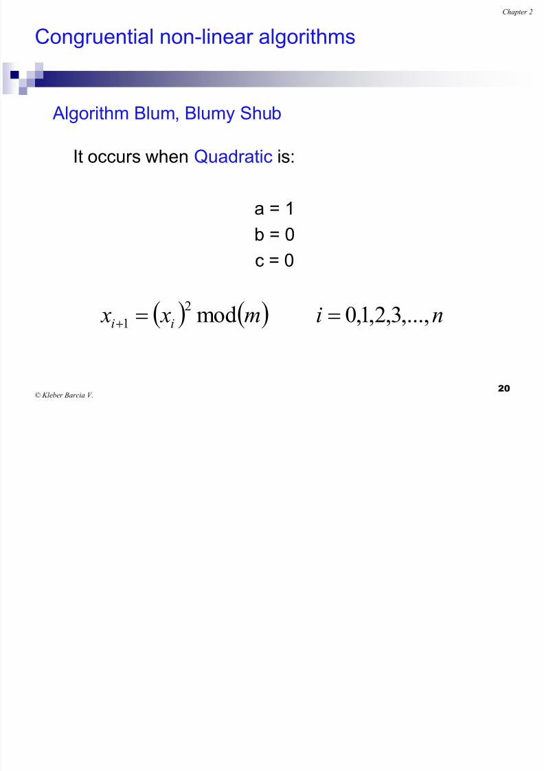
Congruential non-linear algorithms
Algorithm Blum, Blumy Shub
It occurs when Quadratic is:
a = 1
b = 0
c = 0
nim x x ii ,...,3,2,1,0 mod2
1
h

8/20/2019 2 Random Numbers (1)
http://slidepdf.com/reader/full/2-random-numbers-1 21/47
© Kleber Barcia V.
Chapter 2
21
Characteristics of a good generator
Maximum Density Such that the values assumed by R i , i = 1,2,…, leave no large
gaps on [0,1]
Problem: Instead of continuous, each R i is discrete
Solution: a very large integer for modulus m
Maximum Period
To achieve maximum density and avoid cycling.
Achieve by: proper choice of a, c , m, and X 0 .
Most digital computers use a binary representation ofnumbers
Speed and efficiency depend on the modulus, m, to be (or close
to) 2b
a big number Rev. 1
Ch 2

8/20/2019 2 Random Numbers (1)
http://slidepdf.com/reader/full/2-random-numbers-1 22/47
© Kleber Barcia V.
Chapter 2
22
Tests for Random Numbers
Two categories:
Testing for uniformity:
H 0 : R i ~ U[0,1]
H 1: R i ~ U[0,1]
Test for independence:H 0 : R i ~ independently
H 1: R i ~ independently
Mean test
H0: µri = 0.5H1: µri = 0.5
We can use the normal distribution with σ2 = 1/12
or σ = 0.2887 with a significance level α = 0.05
/
/
/
Ch t 2
8/20/2019 2 Random Numbers (1)
http://slidepdf.com/reader/full/2-random-numbers-1 23/47
© Kleber Barcia V.
Chapter 2
23
Tests for Random Numbers
When to use these tests:
If a well-known simulation languages or random-number
generators is used, it is probably unnecessary to test
If the generator is not explicitly known or documented, e.g.,
spreadsheet programs, symbolic/numerical calculators, testsshould be applied to the sample numbers.
Types of tests:
Theoretical tests: evaluate the choices of m, a, and c without
actually generating any numbers
Empirical tests: applied to actual sequences of numbers
produced. Our emphasis.
Rev. 1
Ch t 2
8/20/2019 2 Random Numbers (1)
http://slidepdf.com/reader/full/2-random-numbers-1 24/47
© Kleber Barcia V.
Chapter 2
24
Kolmogorov-Smirnov test [Uniformity Test]
Very useful for little data.
For discrete and continuous variables.
Procedure:
1. Arrange the r i from lowest to highest
2. Determine D+, D-
3. Determine D4. Determine the critical value of Dα, n
5. If D> Dα, n then r i are not uniform
Chapter 2

8/20/2019 2 Random Numbers (1)
http://slidepdf.com/reader/full/2-random-numbers-1 25/47
© Kleber Barcia V.
Chapter 2
25
Kolmogorov-Smirnov test [Uniformity Test]
Example: Suppose that 5 generated numbers are 0.44,0.81, 0.14, 0.05, 0.93.
Step 1:
Step 2:
Step 3: D = max(D + , D - ) = 0.26
Step 4: Fora = 0.05 ,
D a
n = 0.565 > D
So not reject H 0 .
Sort R (i) Ascending
D+ = max {i/N – R (i) }
D- = max {R (i) - (i-1)/N}
R (i) 0.05 0.14 0.44 0.81 0.93
i/N 0.20 0.40 0.60 0.80 1.00
i/N – R (i) 0.15 0.26 0.16 - 0.07R (i) – (i-1)/N 0.05 - 0.04 0.21 0.13
Chapter 2

8/20/2019 2 Random Numbers (1)
http://slidepdf.com/reader/full/2-random-numbers-1 26/47
© Kleber Barcia V.
Chapter 2
26
Chi-square test [Uniformity Test]
The Chi-square test uses the statistical sample:
Approximately the chi-square distribution with n-1 degrees of
freedom is tabulated in Table A.6
For a uniform distribution, the expected number Ei, in each class
is:
Valid only for large samples, example: N> = 50
If X02>X2
(α; n-1) reject the hypothesis of uniformity
n
i i
ii
E
E O
1
22
0
)(
nobservatioof #totaltheis N where,n N E i
n is the # of classes
Oi is the observed # of
the class i th
E i is the expected # of
the class i th
Chapter 2

8/20/2019 2 Random Numbers (1)
http://slidepdf.com/reader/full/2-random-numbers-1 27/47
© Kleber Barcia V.
Chapter 2
27
Chi-square test [Uniformity Test]
Example: Use Chi-square with a = 0.05 to test that the data shownare uniformly distributed
The test uses n = 10 intervals of equal length:
[0, 0.1), [0.1, 0.2), …, [0.9, 1.0)
0.34 0.90 0.25 0.89 0.87 0.44 0.12 0.21 0.46 0.67
0.83 0.76 0.79 0.64 0.70 0.81 0.94 0.74 0.22 0.74
0.96 0.99 0.77 0.67 0.56 0.41 0.52 0.73 0.99 0.02
0.47 0.30 0.17 0.82 0.56 0.05 0.45 0.31 0.78 0.05
0.79 0.71 0.23 0.19 0.82 0.93 0.65 0.37 0.39 0.42
0.99 0.17 0.99 0.46 0.05 0.66 0.10 0.42 0.18 0.49
0.37 0.51 0.54 0.01 0.81 0.28 0.69 0.34 0.75 0.49
0.72 0.43 0.56 0.97 0.30 0.94 0.96 0.58 0.73 0.05
0.06 0.39 0.84 0.24 0.40 0.64 0.40 0.19 0.79 0.62
0.18 0.26 0.97 0.88 0.64 0.47 0.60 0.11 0.29 0.78
Chapter 2

8/20/2019 2 Random Numbers (1)
http://slidepdf.com/reader/full/2-random-numbers-1 28/47
© Kleber Barcia V.
Chapter 2
28
Chi-square test [Uniformity Test]
The X02 value = 3.4
Compared to the value of Table A.6, X20.05, 9 = 16.9
Then H0 is not rejected.
Intervalo Oi Ei Oi-Ei (Oi-Ei)2
(Oi-Ei)2
Ei
1 8 10 -2 4 0.4
2 8 10 -2 4 0.4
3 10 10 0 0 0.0
4 9 10 -1 1 0.1
5 12 10 2 4 0.4
6 8 10 -2 4 0.4
7 10 10 0 0 0.0
8 14 10 4 16 1.6
9 10 10 0 0 0.0
10 11
100
10
100
1
0
1 0.1
3.4
Chapter 2
8/20/2019 2 Random Numbers (1)
http://slidepdf.com/reader/full/2-random-numbers-1 29/47
© Kleber Barcia V.
Chapter 2
29
Tests for Autocorrelation [Test of Independence]
It is a test between each m numbers, starting with thenumber i The auto-correlation r im between the numbers R i , R i+m, R i+2m,
R i+(M+1)m
M is the largest integer such that, , where N is
the total number of values in the sequence Hypothesis:
If the values are not correlated: For large values of M, the distribution estimation r im, is
approximately a normal distribution.
N )m(M i 1
tindependen NOTarenumbers ,0 :
,0 :
1
0 tindependenarenumbers
im
im
H
H
r
r
Chapter 2
8/20/2019 2 Random Numbers (1)
http://slidepdf.com/reader/full/2-random-numbers-1 30/47
© Kleber Barcia V.
Chapter 2
30
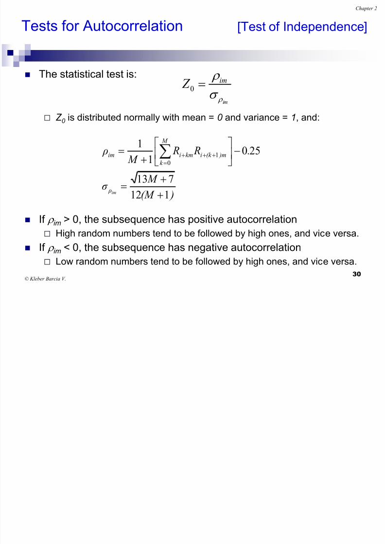
Tests for Autocorrelation [Test of Independence]
The statistical test is:
Z 0 is distributed normally with mean = 0 and variance = 1, and:
If r im > 0, the subsequence has positive autocorrelation
High random numbers tend to be followed by high ones, and vice versa.
If r im < 0, the subsequence has negative autocorrelation
Low random numbers tend to be followed by high ones, and vice versa.
im
im Z r
r
ˆ
0ˆ
ˆ
)(M
M σ
. R R M
ρ
im ρ
M
k
)m(k ikmiim
112
713ˆ
2501
1ˆ
0
1
Chapter 2
8/20/2019 2 Random Numbers (1)
http://slidepdf.com/reader/full/2-random-numbers-1 31/47
© Kleber Barcia V.
Chapter 2
31
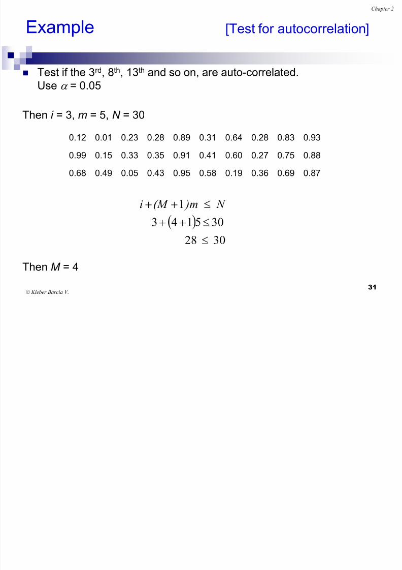
Example [Test for autocorrelation]
Test if the 3rd, 8th, 13th and so on, are auto-correlated.Use a = 0.05
Then i = 3, m = 5, N = 30
Then M = 4
0.12 0.01 0.23 0.28 0.89 0.31 0.64 0.28 0.83 0.93
0.99 0.15 0.33 0.35 0.91 0.41 0.60 0.27 0.75 0.88
0.68 0.49 0.05 0.43 0.95 0.58 0.19 0.36 0.69 0.87
30 28
305143
1
N )m(M i
Chapter 2
8/20/2019 2 Random Numbers (1)
http://slidepdf.com/reader/full/2-random-numbers-1 32/47
© Kleber Barcia V.
p
32
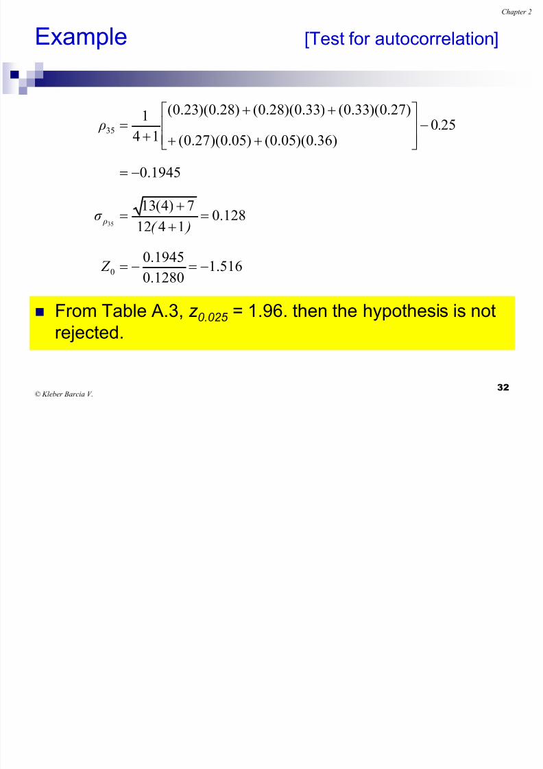
Example [Test for autocorrelation]
From Table A.3, z 0.025 = 1.96. then the hypothesis is not
rejected.
516.11280.0
1945.0
128.01412
7)4(13ˆ
1945.0
250)36.0)(05.0()05.0)(27.0(
)27.0)(33.0()33.0)(28.0()28.0)(23.0(
14
1ˆ
0
35
35
Z
)( σ
. ρ
ρ
Chapter 2

8/20/2019 2 Random Numbers (1)
http://slidepdf.com/reader/full/2-random-numbers-1 33/47
© Kleber Barcia V.
p
33
Other tests of Independence
Test runs up and down Test runs up and below the mean
Test poker
Test series
Test holes
-----HOMEWORK 3 at SIDWeb-----
Bonus: (3 points for the partial exam)
Write a computer program that generates random numbers (4 digits)using the Multiplicative Congruential Algorithm. Allow user to entervalues x0, k, g
Give an example printed and the program file
Chapter 2

8/20/2019 2 Random Numbers (1)
http://slidepdf.com/reader/full/2-random-numbers-1 34/47
© Kleber Barcia V.
p
34
Understand how to generate random variables
from a specific distribution as inputs of a
simulation model.
Illustrate some used techniques for generating
random variables.
Inverse-transform technique
Acceptance- rejection technique
2. Objectives. Random Variables
Chapter 2

8/20/2019 2 Random Numbers (1)
http://slidepdf.com/reader/full/2-random-numbers-1 35/47
© Kleber Barcia V.35
Inverse-transform technique
It can be used to generate random variables from anexponential distribution, uniform, Weibull, triangular and
empirical distribution.
Concept:
For cdf function: r = F(x)
Generate r (0,1)
Find x:
x = F-1(r)
r 1
x1
r = F(x)
Chapter 2
8/20/2019 2 Random Numbers (1)
http://slidepdf.com/reader/full/2-random-numbers-1 36/47
© Kleber Barcia V.36
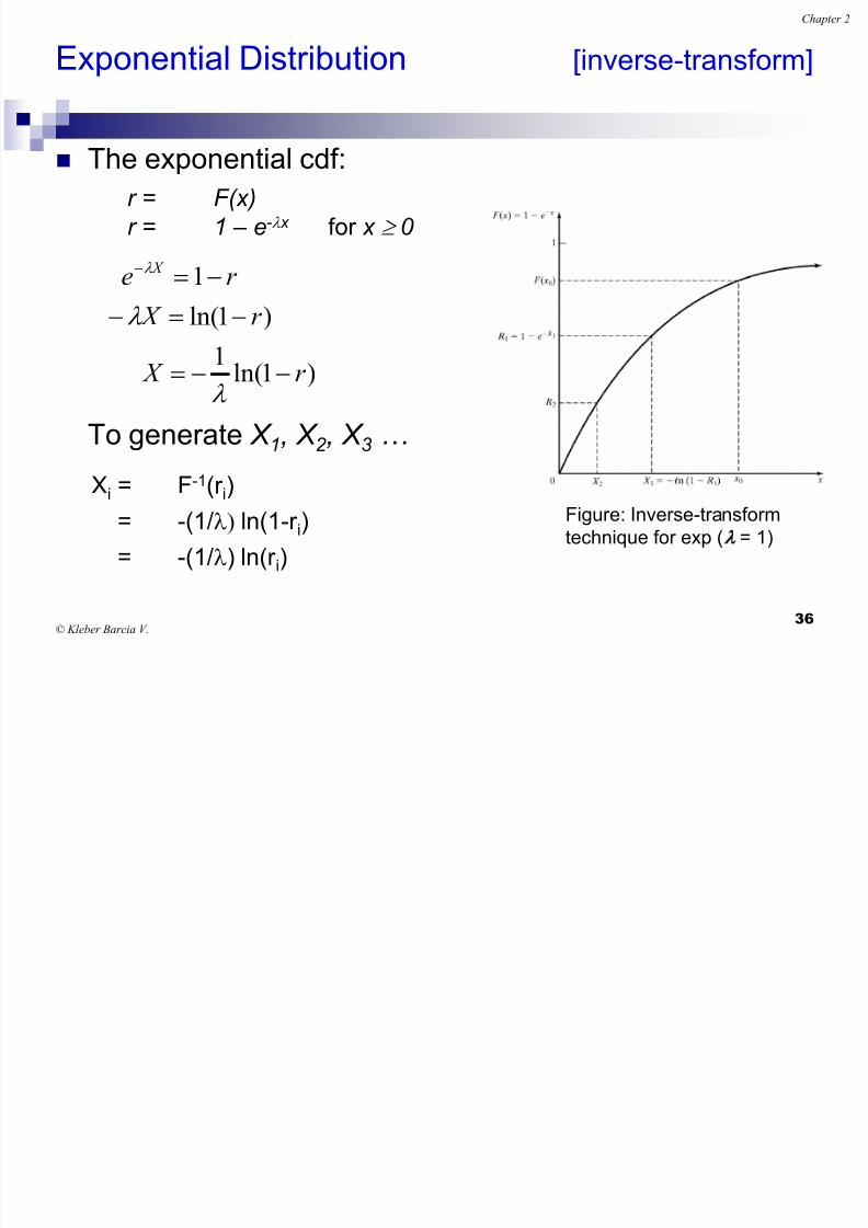
Exponential Distribution [inverse-transform]
The exponential cdf:
To generate X 1, X 2 , X 3 …
r = F(x)
r = 1 – e-l x for x 0
Xi = F-1(r i)
= -(1/l ln(1-r i)
= -(1/l) ln(r i)
Figure: Inverse-transform
technique for exp (l
= 1)
)1ln(1
)1ln(
1
r X
r X
r e X
l
l
l
Chapter 2

8/20/2019 2 Random Numbers (1)
http://slidepdf.com/reader/full/2-random-numbers-1 37/47
© Kleber Barcia V.37
Table of Distributions [inverse-transform]
Distribution Cumulative Inverse-Transform
Uniform
Weibull
Triangular
Normal
b xa
aba x x F
0 1
xe x F
x
a
21 221
10 2
2
2
x x x F
x x x F
ii r aba x
a 1
1ln r x
121 122
210 2
r r x
r r x
z x
Chapter 2
8/20/2019 2 Random Numbers (1)
http://slidepdf.com/reader/full/2-random-numbers-1 38/47
© Kleber Barcia V.38
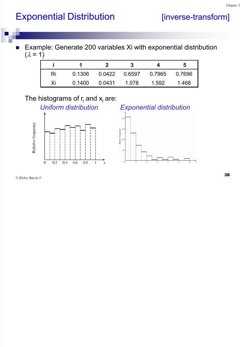
Exponential Distribution [inverse-transform]
Example: Generate 200 variables Xi with exponential distribution(l = 1)
The histograms of r i and xi are:
Uniform distribution Exponential distribution
i 1 2 3 4 5
Ri 0.1306 0.0422 0.6597 0.7965 0.7696
Xi 0.1400 0.0431 1.078 1.592 1.468
Chapter 2

8/20/2019 2 Random Numbers (1)
http://slidepdf.com/reader/full/2-random-numbers-1 39/47
© Kleber Barcia V.39
Uniform Distribution [Example]
The temperature of an ovenbehaves uniformly within the
range of 95 to 100 ° C.
Modeling the behavior of the
temperature.
ii r aba x
Measurements r i Temperature oC
1 0.48 95+5*0.48=97.40
2 0.82 99.103 0.69 98.45
4 0.67 98.35
5 0.00 95.00
Chapter 2

8/20/2019 2 Random Numbers (1)
http://slidepdf.com/reader/full/2-random-numbers-1 40/47
© Kleber Barcia V.40
Exponential Distribution [Example]
Historical data service time a Bankbehaves exponentially with an
average of 3 min / customer.
Simulate the behavior of this
random variable
Customer r i Service Time(min)
1 0.36 3.06
2 0.17 5.313 0.97 0.09
4 0.50 2.07
5 0.21 0.70
ii r x 1ln3
Chapter 2
8/20/2019 2 Random Numbers (1)
http://slidepdf.com/reader/full/2-random-numbers-1 41/47
© Kleber Barcia V.41
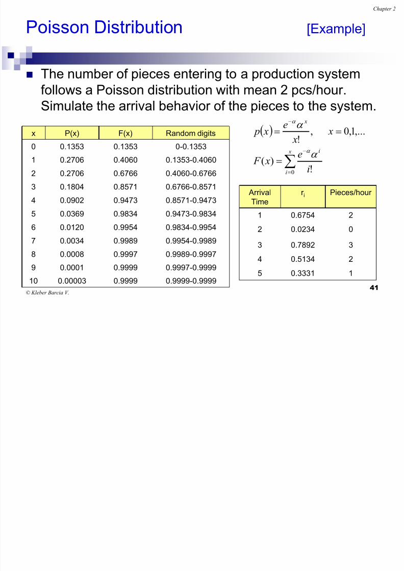
Poisson Distribution [Example]
The number of pieces entering to a production systemfollows a Poisson distribution with mean 2 pcs/hour.
Simulate the arrival behavior of the pieces to the system.
x P(x) F(x) Random digits
0 0.1353 0.1353 0-0.1353
1 0.2706 0.4060 0.1353-0.4060
2 0.2706 0.6766 0.4060-0.6766
3 0.1804 0.8571 0.6766-0.8571
4 0.0902 0.9473 0.8571-0.9473
5 0.0369 0.9834 0.9473-0.9834
6 0.0120 0.9954 0.9834-0.9954
7 0.0034 0.9989 0.9954-0.9989
8 0.0008 0.9997 0.9989-0.9997
9 0.0001 0.9999 0.9997-0.9999
10 0.00003 0.9999 0.9999-0.9999
Arrival
Time
r i Pieces/hour
1 0.6754 2
2 0.0234 0
3 0.7892 3
4 0.5134 2
5 0.3331 1
x
i
i
x
i
e x F
x
x
e x p
0 !)(
,...1,0 ,
!a
a
a
a
Chapter 2
8/20/2019 2 Random Numbers (1)
http://slidepdf.com/reader/full/2-random-numbers-1 42/47
© Kleber Barcia V.42
Convolution Method
In some probability distributions, the random variable
can be generated by adding other random variables
Erlang Distribution
The sum of exponential variables of equal means
(1/λ)
Y = x1+x2+…+xk
Y = (-1/kλ)ln(1-r 1)+ (-1/kλ)ln(1-r 2)+…+ (-1/kλ)ln(1-r k)
Where:
Y = Er i= (-1/kλ)lnπ(1-r i) The factor productoria
Chapter 2

8/20/2019 2 Random Numbers (1)
http://slidepdf.com/reader/full/2-random-numbers-1 43/47
© Kleber Barcia V.43
Convolution Method
The processing time of certain machine follows a 3-erlang distribution with mean 1/λ = 8 min/piece
Y = -(8/3)[lnπ(1-r i)] = -(8/3)ln[(1-r 1) (1-r 2) (1-r 3)]
Piece 1-r 1 1-r 2 1-r 3 Process Time
1 0.28 0.52 0.64 6.328
2 0.96 0.37 0.83 3.257
3 0. 04 0.12 0.03 23.588
4 0.35 0.44 0.50 6.837
5 0.77 0.09 0.21 11.279
Chapter 2

8/20/2019 2 Random Numbers (1)
http://slidepdf.com/reader/full/2-random-numbers-1 44/47
© Kleber Barcia V.44
Empirical continuous distribution [inverse-transform]
When theoretical distribution is not applicable To collect empirical data:
Resample the observed data
Interpolate between observed data points to fill in the gaps
For a small and large sample set (size n):
Arrange the data from smallest to largest
Assign the probability 1/n to each interval
Where 1 / n is the probability
(n)(2)(1) xxx
(i)1)-(i xxx
ni Ra x R F X ii )1()(ˆ
)1(1
n
x x
nin
x xa
iiii
i
/1/)1(/1
)1()()1()(
Chapter 2

8/20/2019 2 Random Numbers (1)
http://slidepdf.com/reader/full/2-random-numbers-1 45/47
© Kleber Barcia V.45
Empirical continuous distribution [inverse-transform]
Example: Suppose that the observed data of 100 repair times of a machineare:
i
Interval
(Hours) Frecuency
Relative
Frecuency
Cumulative
Frecuencia, c i Slot, a i
1 0.25 ≤ x ≤ 0.5 31 0.31 0.31 0.81
2 0.5 ≤ x ≤ 1.0 10 0.10 0.41 5.0
3 1.0 ≤ x ≤ 1.5 25 0.25 0.66 2.0
4 1.5 ≤ x ≤ 2.0 34 0.34 1.00 1.47
Consider r 1 = 0.83:
c3 = 0.67 < r 1 < c4 = 1.00
X1 = x(4-1) + a4(r 1 – c(4-1))
= 1.5 + 1.47(0.83-0.66)
= 1.75
Chapter 2
8/20/2019 2 Random Numbers (1)
http://slidepdf.com/reader/full/2-random-numbers-1 46/47
© Kleber Barcia V.46
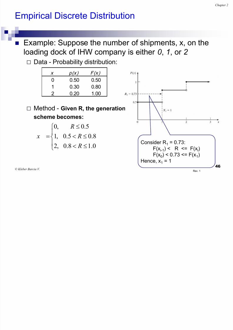
Empirical Discrete Distribution
Example: Suppose the number of shipments, x, on theloading dock of IHW company is either 0 , 1, or 2
Data - Probability distribution:
Method - Given R, the generation
scheme becomes:
0.18.0
8.05.0
5.0
,2
,1
,0
R
R
R
xConsider R1 = 0.73:
F(xi-1) < R <= F(xi)
F(x0) < 0.73 <= F(x1)
Hence, x1 = 1
x p(x) F(x )
0 0.50 0.50
1 0.30 0.80
2 0.20 1.00
Rev. 1
Chapter 2

8/20/2019 2 Random Numbers (1)
http://slidepdf.com/reader/full/2-random-numbers-1 47/47
Acceptance-Rejection technique
Useful particularly when inverse cdf does not exist in closedform, a.k.a. thinning
To generate random variables X ~ U (1/4, 1) we must:
This procedure is only for uniform distributions
Acceptance-rejection technique is also applied to Poisson,nonstationary Poisson, and gamma distributions
-----HOMEWORK 4 at SIDWeb-----
procedure :
Step 1. Generate R ~ U[0,1]Step 2a. If R >= ¼, accept X=R.
Step 2b. If R < ¼, reject R,back to step 1
Generate R
Condition
output R’
si
no