2 Modelling timbre distance with temporal statistics from

2

Modelling timbre distance with temporal

statistics from polyphonic musicFabian Morchen, Alfred Ultsch, Michael Thies, and Ingo Lohken

Abstract

Timbre distance and similarity are an expression of the phenomenon that some music appears similar

while other songs sound very different to us. The notion of genre is often used to categorize music, but

songs from a single genre do not necessarily sound similar and vice versa. In this work we analyze and

compare a large amount of different audio features and psychoacoustic variants thereof for the purpose

of modelling timbre distance. The sound of polyphonic music is commonly described by extracting

audio features on short time windows during which the sound is assumed to be stationary. The resulting

down sampled time series are aggregated to form a high level feature vector describing the music. We

generated high level features by systematically applying static and temporal statistics for aggregation.

The temporal structure of features in particular has previously been largely neglected. A novel supervised

feature selection method is applied to the huge set of possible features. The selected feature distances

correspond to timbre differences in music. The features show few redundancies and have high potential

for explaining possible clusters. They outperform seven other previously proposed feature sets on several

datasets w.r.t. the separation of the known groups of timbrally different music.

I. INTRODUCTION

The raw audio data of polyphonic music is not suited for direct analysis with data mining algorithms.

High quality audio data needs a large amount of memory and contains various sound impressions that

are overlayed in a single (or a few correlated) time series. These time series cannot be compared directly

in a meaningful way. A common technique is to describe the sound by extracting audio features, e.g. for

the classification into musical genre categories [1]. Many features are commonly extracted on short time

windows during which the sound is assumed to be stationary. This produces a down sampled multivariate

Data Bionics Research Group, Philipps-University Marburg, 35032 Marburg, Germany

August 13, 2005 DRAFT

3

time series of sound descriptors. These low level features are aggregated to form a high level feature

vector describing the sound of a song.

Many audio features have been proposed in the literature, but it remains unclear how they relate to each

other. Data mining algorithms will suffer from working with too many and possibly correlated features.

Only few of the proposed features are motivated by psychoacoustics. We analyzed and compared a large

amount of different audio features and psychoacoustic variants thereof for the purpose of modelling

timbre distance. The goal is to select a subset of the features with few redundancies and large distances

between different sounding music.

Only few authors have incorporated the temporal structure of the low level feature time series when

summarizing them to describe the music [2]. Sometimes the moments of the 1st and 2nd order differences

are used [3]. The modulation strength in several frequency bands was calculated in [4] and [5]. We evaluate

a large set of temporal and non temporal statistics for the description of sound. The cross product of the

low level features (see Section IV) and statistical aggregations (see Section V) resulted in a huge set of

mostly new audio features.

Much research has been targeted towards classification of musical genre. The problem with this

approach is the subjectivity and ambiguity of the categorization used for training and validation [2].

Existing genre taxonomies are found to be somewhat arbitrary and hard to compare. Often genres don’t

even correspond to the sound of the music but to the time and place where the music came up or the

culture of the musicians creating it. Some authors try to explain the low performance of their classification

methods by the fuzzy and overlapping nature of genres [1]. An analysis of musical similarity showed

bad correspondence with genres, again explained by their inconsistency and ambiguity [6]. Looking at

all these findings, the question is raised whether genre classification from sound properties even makes

sense, if there can be similar sounding pieces in different genres. Similar problems are present for artist

similarity [7]. In [2] the dataset is therefore chosen to be timbrally consistent irrespectively of the genre.

But even for timbre similarity an upper bound for the retrieval performance is observed.

We decided to take a different approach similar to [5]. Our goal was to visualize and cluster a music

collection with U-Map [8] displays of Emergent Self-organizing Maps (ESOM) [9], [10] based on timbre

differences of the sound. The ESOM visualization capabilities are based on the map paradigm and enable

intuitive navigation of high dimensional feature spaces. Possible clusters should correspond to different

sounding music, independently of what genre a musical expert would place it in. The clusters, if there

are any, can still correspond to something like a genre or a group of similar artists. Outliers can be

identified and transitions between overlapping clusters will be visible. Note, that the aim of achieving


4

large distances of feature vectors extracted from different sounding music is not equivalent to that of

having high classification accuracy. We developed a supervised feature selection method that is targeted

towards selecting features that create large distances or large density differences between feature vectors

from different sounding music.

In summary, our contributions are as follows

• Proposal of some novel low level features and variants of existing features.

• Consistent and systematic use of static and temporal statistics for aggregation of low level features

to form high level features.

• Supervised feature selection from about 66,000 possible sound descriptors for modelling timbre

distance (obtained by the cross product of low level features and high level aggregations).

First some related work is discussed in Section II in order to motivate our approach. The datasets are

described in Section III. The low level features and variants we have used will be explained in Section IV.

Section V lists the large set of aggregations used to create the high level features. The methods we propose

for the analysis, selection, and evaluation of the features are described in Section VI. The results are

presented in Section VII. The results of this study are discussed in Section VIII. An application of

the audio features to visualizing music collections is described in Section IX. A summary is given in

Section X.

II. RELATED WORK AND MOTIVATION

The origins of research on musical similarity are in information retrieval [11]. An early approach tried

to classify artists [12] with Mel Frequency Cepstral Coefficients (MFCC) (e.g. [13]).

More directly targeted towards musical similarity is [14] and [15]. Both use a large set of MFCC feature

vectors for the representation of each song by mixture models. An architecture for large scale evaluation

of audio similarity based on these bag of frames [16] methods is described in [17]. Large similarity

matrices for the pairwise comparison of songs need to be stored in addition to the song models. The

model based representation makes distance calculations between songs problematic. They cannot easily

be used with data mining algorithms requiring the calculation of a centroid. It also scales badly with the

number of songs, even though the study is motivated by “millions of music titles [...] available to millions

of users” [17]. The addition of a single song to a database requires the comparison of the new song’s

model to all existing models. Vector based distance calculations are much faster and many clustering

algorithms do not require pairwise distance calculations.


5

The seminal work of Tzanetakis [1], [18] is the foundation for most research in musical genre

classification. A single feature vector is used to describe a song, opening the problem for many standard

machine learning methods. Based on 19 timbral, 6 rhythmic [19] and 5 pitch features [20] Gaussian

classifiers are trained on 100 songs from 10 main musical genres and some sub-genres. The classification

accuracy reported is 66%. Misclassification e.g. among sub-genres of jazz are explained due to similar

sounding pieces. Note, that when using clustering and visualization this will not be a problem. If pieces

sound similar, they should be close, no matter which sub genre they belong to.

Many follow-ups of this approach tried to improve it by using different features and/or different classi-

fiers. For example wavelet based features with Support Vector Machines (SVM) and Linear Discriminant

Analysis (LDA) [21] or linear predictive coefficients (LPC) and SVM [22]. In [4] four feature sets are

compared with Quadratic Discriminant Analysis. In order to reduce the dimensionality, feature ranking

based on the Bhattacharyya distance is used. Using the temporal behavior of low level features turned

out to be important.

The composition of feature extractors from (audio) time series is formalized in [23]. Genetic pro-

gramming is used to generate good features for classification of genre and personal taste. The fitness is

evaluated using the accuracy of SVM training with genetic feature selection. Some well known features

were rediscovered and some new features based on non-linear time series analysis were found. A similar

approach is taken in [24], but targeted towards more general description of acoustic signals, not musical

genre.

Distance measures based on vectors of audio features are evaluated in [6] on a large set of songs. The

Spectrum Histograms were found to perform best. The best correspondence was achieved with albums,

less with artists, and worst for genres.

A first step away from strict classification towards visualization of music based on intrinsic sound

features is taken in [25]. An early approach using SOM is [5]. The maps are rather small, however. This

results in a k-Means like procedure [26]. For the emergence of higher level structure, larger ESOMs

are needed. The Smoothed Data Histograms (SDH) [27] visualization used in [5] represents an indirect

estimation of the high dimensional probability density. We use the Pareto Density Estimation (PDE) [28],

a more direct estimator based on information optimal sets and distance based visualizations.

The feature vectors used in [5], [6], [29] are very high dimensional. This is problematic for distance

calculations because these vectors spaces are inherently empty [30]. Interest in visualization of music

collections seems to be increasing. Recently, approaches based on collaging [31], discs, rectangles and

tree maps [32], and graph drawing [33] have been proposed.


6

III. DATA

We created three disjoint data sets for the selection and validation of features modelling timbre distance.

Our motivation for composing these sets of music was to avoid genre categories and create clusters of

similar sounding pieces within each group, while achieving high timbre distances between songs from

different groups. The consistency of the groups was determined by a consensus of 10 listeners with

different musical tastes.

Relying on genre categorizations from websites as the ground truth for different sounding music is

problematic. Songs from the same genre may have a low timbre similarity and vice versa. Often genre

categories are attached to an artist and do not reflect the sound of a particular album or even song. The

albums created by Queen over the years show a variety of different musical styles. The early albums of

Radiohead contained Alternative Rock, while the recent publications are heavily influenced by electronic

music. Artists like the Beastie Boys or Ben Harper created many songs that completely break out of

the genre they are typically associated with. Songs by the Beastie Boys are typically Hiphop pieces, but

they have also created Punk Rock songs (Heart Attack Man) or Rock songs (I Don’t Know). The album

Diamonds On The Inside by Ben Harper contains music that the authors would classify as Blues (When

It’s Good), Hardrock (So High, So Low), Country (Diamonds On The Inside), Funk (Bring The Funk),

Reggae (With My Own Two Hands), Gospel (Picture Of Jesus), and more.

A. Training data

The training data serves as the ground truth of timbre similarity. We tried to avoid any ambiguity and

selected 200 songs in five timbrally consistent but very different groups and will refer to this dataset as

5G.

The Acoustic group contains songs mainly played by acoustic guitars with few percussion and singing.

The tempo of all songs may be described as slow and the mood as non-aggressive. The artists of these

similar sounding pieces are typically associated with a variety of so called genres: Alternative (Beck),

Blues (John Lee Hooker), Country (Johnny Cash), Grunge (Stone Temple Pilots), Rock (Bob Dylan, The

Beatles, Lenny Kravitz), and even Rap (Beastie Boys).

The pieces in the Classic group were mostly written before the 20th century and composed for orchestra.

The variety of pieces reaches from symphonies, over opera to fugues. Since variations in instrumentation

exist even in one single piece, the Classic is not as timbrally consistent as the other groups. The different

styles include Baroque (Bach), Classic (Mozart, Beethoven), Jazz influenced (Gershwin), and Opera

(Wagner).


7

The most genre label compliant group is Hiphop. Criteria for similarity in this group were strong beats

and rhythmic speaking or singing. Most pieces also contain electronically post processed sample loops.

Artists in this group include Cypress Hill, Run DMC, Ice - T, Die Fantastischen Vier, and Terranova.

The instrumentation of the Metal class is mainly electric guitars, drums, and aggressive singing. The

genres represented by the artists in this group include Heavy Metal (Metallica), Crossover (Rage Against

the Machine), Stoner Rock (Queens of the Stone Age), Alternative Rock (Audioslave), and Industrial

(Ministry).

All pieces in the Electronic group are mainly created with electronic devices and contain samples

processed with electronic effects. Genre labels which might be suitable for different pieces in this group

are House (Cassius), Breakbeats (Chemical Brothers), Techno (Sven Vaeth), and Drum & Bass (Red

Snapper).

B. Validation data

Two different datasets are used for the validation of our approach. They contain many additional

timbrally consistent groups of music to test whether the timbre model obtained from the training data

scales to different music. The 8G data consist of 140 songs in eight timbre groups corresponding to:

Alternative Rock, Stand-up Comedy, German Hiphop, Electronic, Jazz, Oldies, Opera, and Reggae. The

28G data contains 538 songs in 28 roughly equally represented groups: Alternative, Bigband, Bigbeat,

Blues, Boogie, Breakbeat, Classic, Country, Disco, Drum & Bass, Dub, Electronic, Funk, Grunge, US

Hiphop, German Hiphop, House, Jazz, Metal, Pop, Punk, Reggae, Rock ’n’ Roll, Rocksteady, Ska, Soul,

Techno, and Triphop. In contrast to the other data sets a clear distinction between the sounds from any

two groups cannot always be made. This dataset was chosen to represent a personal music collection in

a more realistic way than 5G and 8G.

C. Genre data

The last dataset is the Musical Audio Benchmark (MAB) dataset collected by Mierswa et al.1. 10s

excerpts of each song were made available 2. There are 7 genre groups determined by the labeling given

on the website: Alternative, Blues, Electronic, Jazz, Pop, Rap, and Rock. This dataset was chosen to check

how well the timbre features can distinguish genres and to provide values for performance comparison

based on publically available data.

1from www.garageband.com

2http://www-ai.cs.uni-dortmund.de/audio.html


8

IV. LOW LEVEL FEATURE EXTRACTION

We briefly list all low level features that will later be used to form higher level features. We selected

audio descriptors that can be calculated on short time windows. The audio data was reduced to mono

and a sampling frequency of 22kHz. To reduce processing time and avoid lead in and lead out effects,

a 30s segment from the center of each song was extracted. The window size was 23ms (512 samples)

with 50% overlap. Thus for each low level feature, a time series with 2582 time points at a sampling

rate of 86Hz was produced.

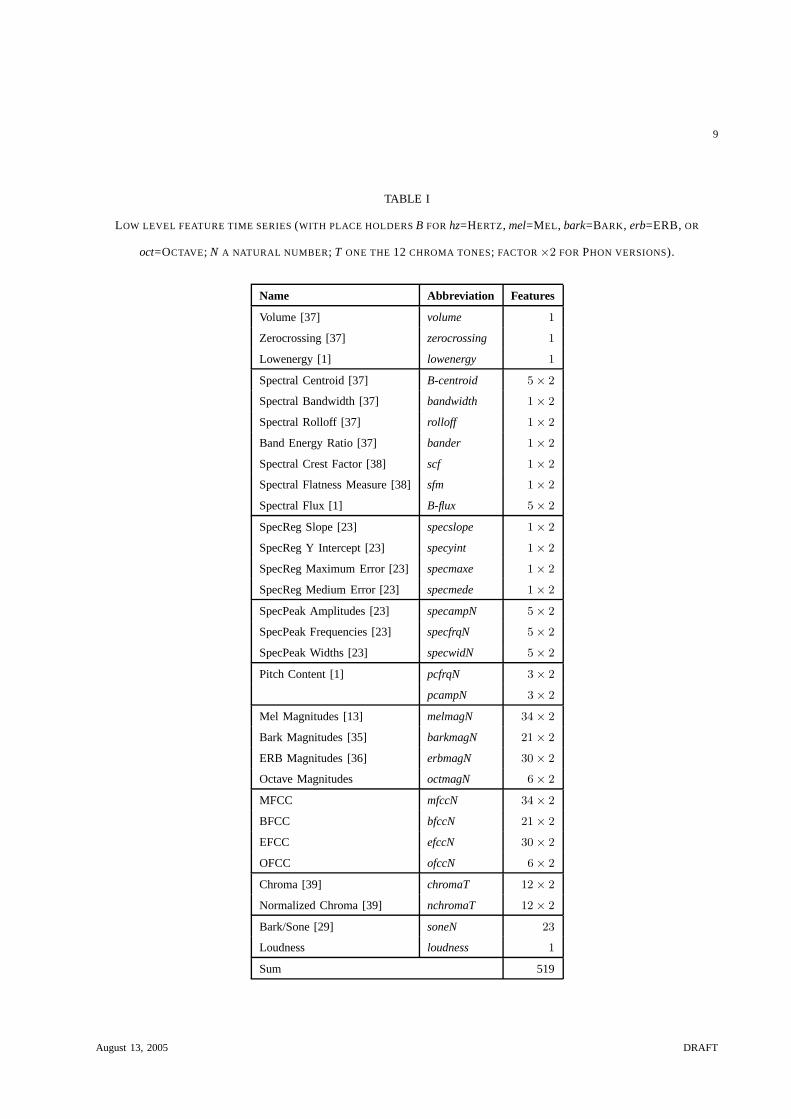
All short term features are listed in Table I with the number of values they produce. For more details

on the features please refer to the original publications listed or [34]. Including the variants created by

applying the Phon weighting to the spectrum prior to further calculations, a total of 518 feature time

series is extracted from each song.

Several novel features are included. We generalized Lowenergy [1] to short time frames: we counted

the percentage of sample amplitudes that were smaller than the RMS on each window. Similarily, we

used the positions and amplitudes of the three most prominent MIDI notes needed for the high level

Pitch Content [20] feature as low level values. In addition to the Mel scale, we created variants of the

MFCC using the Bark [35], Equivalent Rectangular Bandwidth (ERB) [36], and Octave scales.

V. HIGH LEVEL (TEMPORAL) STATISTICS

The most popular way of aggregating a low level feature time series is the usage of mean and standard

deviation. But this is by far not the only way of describing the structure of a time series and not

necessarily the most discriminative for musical sounds. Therefore we explored a large set of static and

temporal statistics for this purpose.

The most simple static aggregations are the first four moments (mean, standard deviation, skewness,

and kurtosis) of the probability distribution of the feature values. These statistics are not robust against

extreme values, however. Therefore we also used the median and the median absolute deviation (MAD)

and robust estimates of the first four moments by removing the largest and smallest 2.5% of the data

prior to estimation. To introduce some temporal structure we also applied the first six of these statistics

to the first and second order differences.

To capture the correlation structure the autocorrelation function (ACF) and the partial autocorrelation

function (PACF) were calculated up to lag 20. The values for lags one to ten (maximum distance of about

200ms) were used as descriptors. Further, the decay of the correlation functions was estimated with the


9

TABLE I

LOW LEVEL FEATURE TIME SERIES (WITH PLACE HOLDERS B FOR hz=HERTZ, mel=MEL, bark=BARK, erb=ERB, OR

oct=OCTAVE; N A NATURAL NUMBER; T ONE THE 12 CHROMA TONES; FACTOR ×2 FOR PHON VERSIONS).

Name Abbreviation Features

Volume [37] volume 1

Zerocrossing [37] zerocrossing 1

Lowenergy [1] lowenergy 1

Spectral Centroid [37] B-centroid 5 × 2

Spectral Bandwidth [37] bandwidth 1 × 2

Spectral Rolloff [37] rolloff 1 × 2

Band Energy Ratio [37] bander 1 × 2

Spectral Crest Factor [38] scf 1 × 2

Spectral Flatness Measure [38] sfm 1 × 2

Spectral Flux [1] B-flux 5 × 2

SpecReg Slope [23] specslope 1 × 2

SpecReg Y Intercept [23] specyint 1 × 2

SpecReg Maximum Error [23] specmaxe 1 × 2

SpecReg Medium Error [23] specmede 1 × 2

SpecPeak Amplitudes [23] specampN 5 × 2

SpecPeak Frequencies [23] specfrqN 5 × 2

SpecPeak Widths [23] specwidN 5 × 2

Pitch Content [1] pcfrqN 3 × 2

pcampN 3 × 2

Mel Magnitudes [13] melmagN 34 × 2

Bark Magnitudes [35] barkmagN 21 × 2

ERB Magnitudes [36] erbmagN 30 × 2

Octave Magnitudes octmagN 6 × 2

MFCC mfccN 34 × 2

BFCC bfccN 21 × 2

EFCC efccN 30 × 2

OFCC ofccN 6 × 2

Chroma [39] chromaT 12 × 2

Normalized Chroma [39] nchromaT 12 × 2

Bark/Sone [29] soneN 23

Loudness loudness 1

Sum 519


10

Fig. 1. Processing steps to obtain optimized audio features from raw audio on training data.

slope of a linear regression line. Finally, the cut point of this regression line with the 5% significance

level of the correlation coefficients was used.

The spectral behavior provides more (even though related) information about the feature time series.

The spectral centroid and bandwidth as well as regression parameters (similar to Section IV for sound

spectra) were estimated. Further, the first 5 cepstral coefficients were obtained.

As in [4] the modulation energy was measured in three frequency bands: “1-2Hz (on the order of

musical beat rates), 3-15Hz (on the order of speech syllabic rates) and 20-43Hz (in the lower range

of modulations contributing to perceptual roughness)”. The absolute values were complemented by the

relative strengths obtained by dividing through the sum of all three.

Non-linear analysis of time series offers an alternative way of describing temporal structure that is

complementary to the analysis of linear correlation and spectral properties. The reconstructed phase

space [40] was utilized in [23] to extract features directly from the audio data. The mean and standard

deviations of the distances and angles in the phase space with an embedding dimension of two and unit

time lag were used. We applied these measures to the feature time series. We further tried higher time

lags, because the lag is commonly suggested to be chosen as the first zero of the autocorrelation function

[41]. We simply tried lags one to ten. In addition to mean and standard deviation of the phase space

features we added skew and kurtosis. A principal component analysis of the phase space was used to

describe the spread of points using the first two eigenvalues of the covariance matrix.

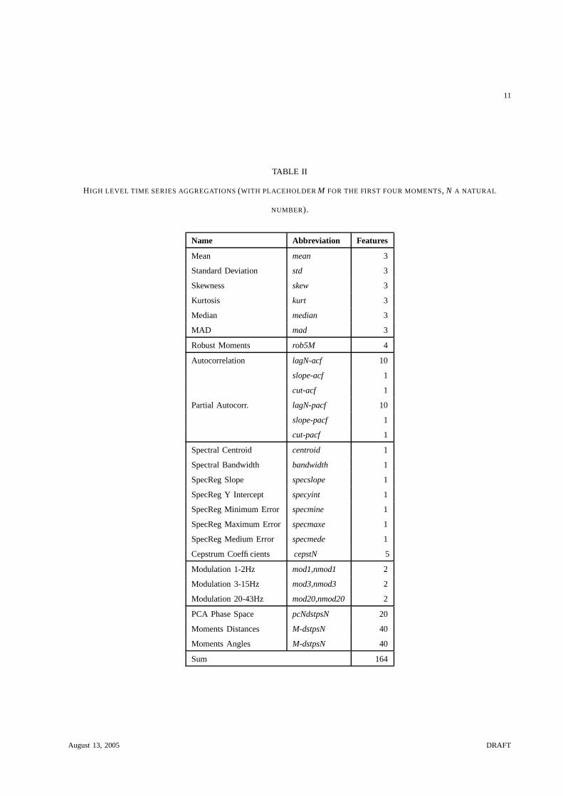
All high level aggregations are listed in Table II with the number of values they produce. A total of

164 features is generated for each low level time series.

VI. METHODS FOR MODELLING TIMBRE DISTANCE

This section describes the remaining steps (see Figure 1) we have taken to obtain high level audio

features with few redundancies providing a good representation of timbre (dis-)similarity. We describe

the preprocessing, the quality scores, and the feature selection performed on the training data. In addition,

the quality measure used for the evaluation of all feature sets on all datasets is motivated and described.


11

TABLE II

HIGH LEVEL TIME SERIES AGGREGATIONS (WITH PLACEHOLDER M FOR THE FIRST FOUR MOMENTS, N A NATURAL

NUMBER).

Name Abbreviation Features

Mean mean 3

Standard Deviation std 3

Skewness skew 3

Kurtosis kurt 3

Median median 3

MAD mad 3

Robust Moments rob5M 4

Autocorrelation lagN-acf 10

slope-acf 1

cut-acf 1

Partial Autocorr. lagN-pacf 10

slope-pacf 1

cut-pacf 1

Spectral Centroid centroid 1

Spectral Bandwidth bandwidth 1

SpecReg Slope specslope 1

SpecReg Y Intercept specyint 1

SpecReg Minimum Error specmine 1

SpecReg Maximum Error specmaxe 1

SpecReg Medium Error specmede 1

Cepstrum Coefficients cepstN 5

Modulation 1-2Hz mod1,nmod1 2



PCA Phase Space pcNdstpsN 20

Moments Distances M-dstpsN 40

Moments Angles M-dstpsN 40

Sum 164


12

A. Preprocessing

In the research of of musical genre classification little emphasis has been taken on the preprocessing

of features. Analyzing the probability distribution for skewed variables and the correlation structure of

the features for redundancies is not overly important for many classifiers. It is crucial, however, for a

meaningful distance calculation between feature vectors to avoid dominance or undesired emphasis of

certain features. In the context of musical genre classification and other applications the low level features

are usually aggregated with the first few moments of the empirical probability distribution. Taking the

mean of a skewed distribution is not representative, however. We propose a careful examination of the

feature distribution. In case of a skewed shape a transformation of the features is sought such that mean

and variance are intuitive descriptions of the distribution. This reduces the skew common to all datasets

and emphasizes remaining and possibly discriminating differences in the distributions.

After an individual analysis of each low level feature, the correlation between the feature time series

needed to be analyzed. Most high level aggregation will be correlated and redundant if they are applied

to two highly correlated low level feature time series. This may introduce unwanted emphasis of this

aspect of the sound. Many data mining algorithms will suffer from working with too many and possibly

correlated inputs. We used the Pearson correlation coefficient of the low level time series to detect highly

correlated features.

B. Quality scores

For the selection of audio features a quality score measuring the ability of a single feature to distinguish

timbre groups was needed. Our intention was to create large distances between timbrally different

sounding musical pieces. Low distances should be produced for similar sounds of the training dataset.

Thus, a measure for separation of one class from the remaining classes is necessary. The separation ability

of a single feature can be visualized with probability density estimates of one group vs. the remaining

groups. Figure 2 shows the PDE [28] for a single feature and the Electronic group vs. all other groups.

The PDE is a fixed width kernel density estimation. The radius is chosen in a data adaptive way to

produce information optimal sets that correspond to the Pareto 80/20 rule.

It can be seen that the values of this feature for songs from the Electronic group are likely to be

different from other songs, because there is few overlap of the two densities. Using this feature as one

component of a feature vector describing each song will significantly contribute to large distance of the

Electronic group from the rest. This intuition is formulated as a quality measure: The Separation score

is calculated as one minus the area under the minimum of both probability density estimates (shown


13

0.15 0.2 0.25 0.3 0.35 0.4 0.45 0.50

1

2

3

4

5

6

7

8

9

2nd CC 7th Sone Band

Like

lihoo

d

ElectronicDifferent musicML DecisionError

Fig. 2. PDE for feature with good separation of Electronic music from other timbre groups.

shaded in Figure 2). If the empirical densities are well separated, the area will be close to zero and the

score achieves a value close to one. If both densities are very similar, the score will be close to zero.

The score is inversely proportional to the error made by Maximum Likelihood decision.

The separation score was calculated for each timbre group vs. the remaining groups. This creates five

quality scores per feature on our training data. There are several ways to combine these values in a single

quality score. The maximum of the scores for each class describes the best performance of the feature in

achieving high inter-class distances, we call this the Specialist score (SP). The mean of the five values is

a score for the overall performance of the feature in separating all classes from each other. We call this

the Allrounder score (AR). Obviously there is a tradeoff between specialization and overall performance,

both properties are desirable. We combined both scores in the following way: We normalized both AR

and all five SP scores by their respective maxima over all features to get comparable numbers. The

distance from (0,0) to the coordinates of the relative AR and the best relative SP score, divided by√

2

(the maximum possible value) is defined to be the Pareto score (PS). The naming is done in the spirit of

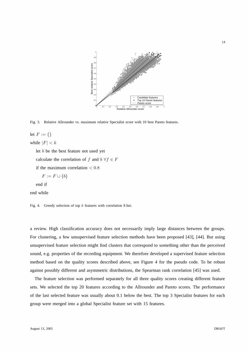
Pareto optimal sets, i.e. the set of all features that are dominated in at most one score. Figure 3 shows a

scatter plot of the relative AR and SP scores and the 10 best features according to the ranking described

below. The Pareto score values are shown by the lines originating in (0,0).

C. Feature selection

The cross product of the low level features and the statistics creates a large amount of high level

candidate features for the goal of modelling timbre distance and makes a feature selection necessary.

Most feature selection techniques are supervised and optimize the accuracy of a classifier, see [42] for


14

0 0.1 0.2 0.3 0.4 0.5 0.6 0.7 0.8 0.9 10

0.1

0.2

0.3

0.4

0.5

0.6

0.7

0.8

0.9

1

Relative Allrounder score

Bes

t rel

ativ

e S

peci

alis

t sco

re

Candidate featuresTop 10 Pareto featuresPareto score

Fig. 3. Relative Allrounder vs. maximum relative Specialist score with 10 best Pareto features.

let F := {}while |F | < k

let b be the best feature not used yet

calculate the correlation of f and b ∀f ∈ F

if the maximum correlation < 0.8

F := F ∪ {b}end if

end while

Fig. 4. Greedy selection of top k features with correlation filter.

a review. High classification accuracy does not necessarily imply large distances between the groups.

For clustering, a few unsupervised feature selection methods have been proposed [43], [44]. But using

unsupervised feature selection might find clusters that correspond to something other than the perceived

sound, e.g. properties of the recording equipment. We therefore developed a supervised feature selection

method based on the quality scores described above, see Figure 4 for the pseudo code. To be robust

against possibly different and asymmetric distributions, the Spearman rank correlation [45] was used.

The feature selection was performed separately for all three quality scores creating different feature

sets. We selected the top 20 features according to the Allrounder and Pareto scores. The performance

of the last selected feature was usually about 0.1 below the best. The top 3 Specialist features for each

group were merged into a global Specialist feature set with 15 features.


15

D. Evaluation

The comparison of the newly created feature sets for their ability of clustering and visualizing different

sounding music was performed using a measure independent from the ranking scores: the ratio of the

median of all inner cluster distances to the median of all pairwise distances. One minus this ratio is

called the distance score (DS). A value close to zero indicates, that songs in the same group are hardly

distinguishable from songs in other groups. Greater values point towards larger inter cluster distances. A

similar measure was used in [6] to compare five feature sets for the ability to distinguish artists, albums,

and genres. We use the difference of the ratio to one to make the score more intuitive and consistent

with the ranking scores above. All datasets were normalized to zero mean and unit standard deviation to

remove influences from differently scaled variables.

VII. RESULTS

A. Preprocessing of low level features

We briefly describe the preprocessing of the low level features, see [34] for more details. We have

analyzed the empirical probability distributions of all low level features described in Section IV on

the 5G dataset. For skewed variables logarithmic or square root transformations were applied. Both

versions were kept to see whether the transformation was really useful for the higher level features. A

comparison of Phon weighted versions of features revealed little influence of the weighting for most

of them. Some interesting feature correlations were discovered, e.g. Rolloff and MFCC2 with a strong

negative correlation. This can be explained by the shape of the cosine function corresponding the 2nd

MFCC that starts with one on the left end of the spectrum, passes 0 in the middle and is negative one

on the right hand side. The more energy is present in the low frequencies, the lower the Rolloff and the

higher the MFCC2 and vice versa. Using many ways of describing the short term spectrum one needs to

be aware of the high correlations among some of them. It is difficult, however, to exclude features based

on the correlation results, because it is unclear which one is better. We therefore deferred the decision to

the feature selection that uses a correlation filter. Only the Phon version with very high correlation were

dropped. This resulted in 402 low level feature time series per song.

B. Selection of high level features

The cross product of the 164 statistics and the 402 low level features creates the huge amount of

65,928 candidate features for the modelling of timbre distance. We will briefly discuss the results of the

feature selection according to the three quality scores, see [34] for more details.


16

0.1 0.2 0.3 0.4 0.5 0.6 0.7 0.80

2

4

6

8

10

12

Like

lyho

od

Values

AcousticElectronicHiphopClassicMetal

Fig. 5. PDE for each timbre group of best Allrounder feature.

The feature selection applied to the Allrounder scores of the features returned root-pc1ps4-root-sone2

as the best performing with a score of 0.62. The feature is obtained as follows: For each sound frame,

the square root of the Sone values in the 2nd Bark band are calculated. The phase space of this feature

time series is reconstructed with dimension two and lag 4. A principal component analysis is performed

and the square root of the largest eigenvalue is the final feature. More simple features are also observed

among the top 20 Allrounders listed in Table VIII. The PDE estimations of the best Allrounder feature for

each musical group are shown in Figure 5. Classical music covers values in the lower range. Right next

to it and partly overlapping is the Acoustic group. The Metal group covers the center values. Electronic

music is largely overlapping with Metal and Hiphop, the latter covering mostly the largest values of the

feature.

The Specialists scores for each group resulted in very different maximum scores, indicating that some

sounds are easier distinguished from the rest than others (see Table III). The best results were achieved

for Classical and Hiphop music with more than 0.9. The best Specialist features for Acoustic and Metal

scored significantly lower at 0.72 and 0.78, respectively. The PDE estimation for Acoustic is shown in

Figure 2, still indicating a strong tendency for separation. The worst best Specialist was observed for

Electronic music.

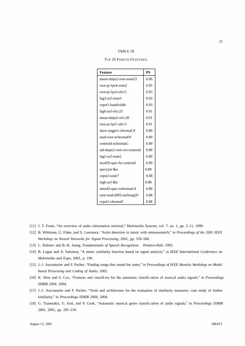
The best feature according to the Pareto score is mean-dstps2-root-sone22 (0.96, mean distance in

phase space of lag 2 of the square root of the 22nd Bark/Sone energy). It also has a high Allrounder

score of 0.58. All Pareto features are listed in Table IX.

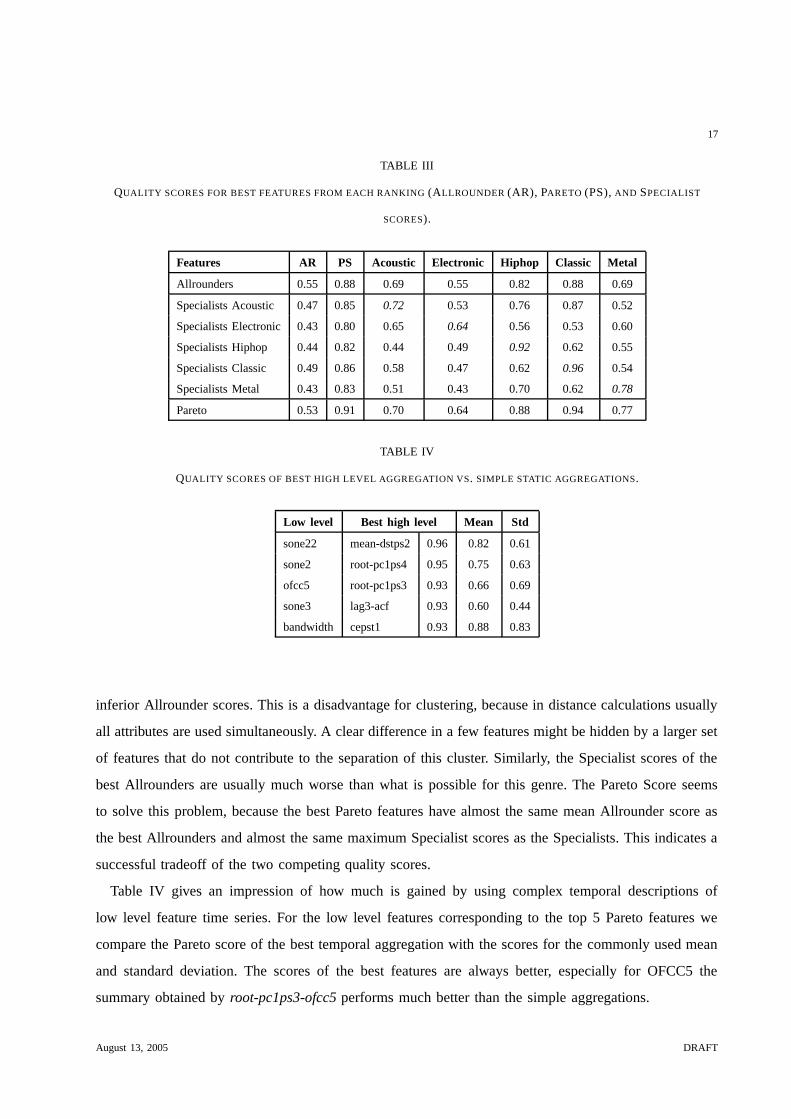
Table III lists the mean Allrounder score (AR), the mean Pareto score (PS), and the maximum Specialist

scores for the top 20 features according to the different quality scores. The winning Specialists have clearly


17

TABLE III

QUALITY SCORES FOR BEST FEATURES FROM EACH RANKING (ALLROUNDER (AR), PARETO (PS), AND SPECIALIST

SCORES).

Features AR PS Acoustic Electronic Hiphop Classic Metal

Allrounders 0.55 0.88 0.69 0.55 0.82 0.88 0.69

Specialists Acoustic 0.47 0.85 0.72 0.53 0.76 0.87 0.52

Specialists Electronic 0.43 0.80 0.65 0.64 0.56 0.53 0.60

Specialists Hiphop 0.44 0.82 0.44 0.49 0.92 0.62 0.55

Specialists Classic 0.49 0.86 0.58 0.47 0.62 0.96 0.54

Specialists Metal 0.43 0.83 0.51 0.43 0.70 0.62 0.78

Pareto 0.53 0.91 0.70 0.64 0.88 0.94 0.77

TABLE IV

QUALITY SCORES OF BEST HIGH LEVEL AGGREGATION VS. SIMPLE STATIC AGGREGATIONS.

Low level Best high level Mean Std

sone22 mean-dstps2 0.96 0.82 0.61

sone2 root-pc1ps4 0.95 0.75 0.63

ofcc5 root-pc1ps3 0.93 0.66 0.69

sone3 lag3-acf 0.93 0.60 0.44

bandwidth cepst1 0.93 0.88 0.83

inferior Allrounder scores. This is a disadvantage for clustering, because in distance calculations usually

all attributes are used simultaneously. A clear difference in a few features might be hidden by a larger set

of features that do not contribute to the separation of this cluster. Similarly, the Specialist scores of the

best Allrounders are usually much worse than what is possible for this genre. The Pareto Score seems

to solve this problem, because the best Pareto features have almost the same mean Allrounder score as

the best Allrounders and almost the same maximum Specialist scores as the Specialists. This indicates a

successful tradeoff of the two competing quality scores.

Table IV gives an impression of how much is gained by using complex temporal descriptions of

low level feature time series. For the low level features corresponding to the top 5 Pareto features we

compare the Pareto score of the best temporal aggregation with the scores for the commonly used mean

and standard deviation. The scores of the best features are always better, especially for OFCC5 the

summary obtained by root-pc1ps3-ofcc5 performs much better than the simple aggregations.


18

C. Evaluation of feature sets

We compared our three feature sets created with the ranking procedure to seven sets of features

previously proposed for musical genre classification or clustering. The most commonly used features are

the MFCC. We chose mean and standard deviation of the first 20 MFCC [3] and the first order differences

[46] and called this feature set MFCC. One of the feature sets used in [4] consists of the modulation

energy in four frequency bands for the first 13 MFCC, we call this McKinney. Note, that all features from

these two sets are subsumed by our process of extracting low level features and applying aggregations.

The feature set from [1] (Tzanetakis) is largely subsumed, but it also contains high level rhythmic and

pitch features extracted in a more complex procedure (Pitch Content, Beat Content). We used the the

Marsyas [47] software3 to extract the 30 dimensional feature set.

The high level features from [6] based on the Bark/Sone representation described in Section IV were

extracted using the available toolbox [48]4: Spectrum Histogram (SH), Periodicity Histograms (PH),

Fluctuation Patterns (FP). The resulting high dimensional features vectors were compressed with PCA

in two variants: keeping the number of components suggested in the original publications and choosing

fewer components according to a scree plot of the eigenvalues indicating the amount of total variance

explained.

The features found with genetic programming in [23], called Mierswa, were extracted using the Yale

[49] software5. The features include simple descriptions of volume and tempo, well known features like

Zerocrossings or SCF, and new features based on regression in the spectrum or phase space representa-

tions.

The distance scores for all feature sets are listed in Table V. Our feature sets all have a distance score

of 0.38 or above, the Pareto features achieve the best value of 0.41. The best of the other feature sets is

McKinney and performs significantly worse at 0.26, closely followed by the modified PH with 0.25. The

fact that McKinney and the modified PH are the best among the rest, might be due to the incorporation

of the temporal behaviour of the low level features. The popular MFCC features with simple temporal

information achieve only 0.16. The worst performing feature set in this experiment were the Spectrum

Histograms with a distance score quite close to zero. This is surprising, because they were found to be the

best features in the evaluation of [6]. As mentioned earlier, one problem with the feature sets by Pampalk

3http://marsyas.sf.net

4http://www.oefai.at/˜elias/ma

5http://yale.sf.net


19

TABLE V

DISTANCE SCORES ON TRAINING DATA.

Features Distance score

Allrounders 0.38

Specialists 0.40

Pareto 0.41

MFCC 0.16

McKinney 0.26

Tzanetakis 0.21

Mierswa 0.12

FP (80PC) 0.10

FP (30PC) 0.20

PH (60PC) 0.07

PH (10PC) 0.25

SH (30PC) 0.05

SH (10PC) 0.12

et al. might be the high dimensionality. The lower dimensional variants always scored better than the

originally proposed number of components. In summary, our feature sets showed superior behavior in

creating small inner cluster and large between cluster distances in the training dataset. Any data mining

algorithms for visualization or clustering will profit from this.

The same feature sets as above were also extracted from the validation datasets to see how well the

concept of timbre similarity translates to different and more musical styles. The distance scores according

to the given clusters are listed in Table VI. The results for the 8G dataset are very similar to the training

data. The new feature sets outperform all other feature sets, the Pareto features are best. The best two

competing feature sets again PH with 10 principal components and McKinney. The absolute numbers of

the distance score are also comparable, indicating no significant loss in performance on the partly very

different music.

The more realistic 28G dataset does not show such a clear clustering tendency anymore. This was to

be expected from the large number and partial similarity of musical groups. Again, the Pareto features

clearly perform best with McKinney being the closest competitor but 25% worse.

The results for the genre data (MAB), also listed in Table VI, were quite surprising. All feature sets

perform badly, the best score of 0.18 is still achieved by the Pareto features. This indicates that the genre

labeling of the datasets probably does not fully correspond to timbrally consistent groups. We checked


20

TABLE VI

DISTANCE SCORES ON VALIDATION AND GENRE DATA.

Features Datasets

8G 28G MAB 8G

Allrounders 0.38 0.20 0.11

Specialists 0.37 0.23 0.17

Pareto 0.42 0.24 0.18

MFCC 0.20 0.12 0.11

McKinney 0.30 0.18 0.13

Tzanetakis 0.24 0.15 0.11

Mierswa 0.16 0.09 0.03

FP (80PC) 0.04 0.04 0.08

FP (30PC) 0.22 0.08 0.09

PH (60PC) 0.07 0.06 0.02

PH (10PC) 0.31 0.13 0.06

SH (30PC) 0.09 0.06 0.04

SH (10PC) 0.18 0.11 0.08

this assumption by listening to parts of the collection. While songs from different genres usually are very

different, we also observed large inconsistencies within the groups. Thus timbre similarity does not seem

to be equivalent to the official genre categories on this data.

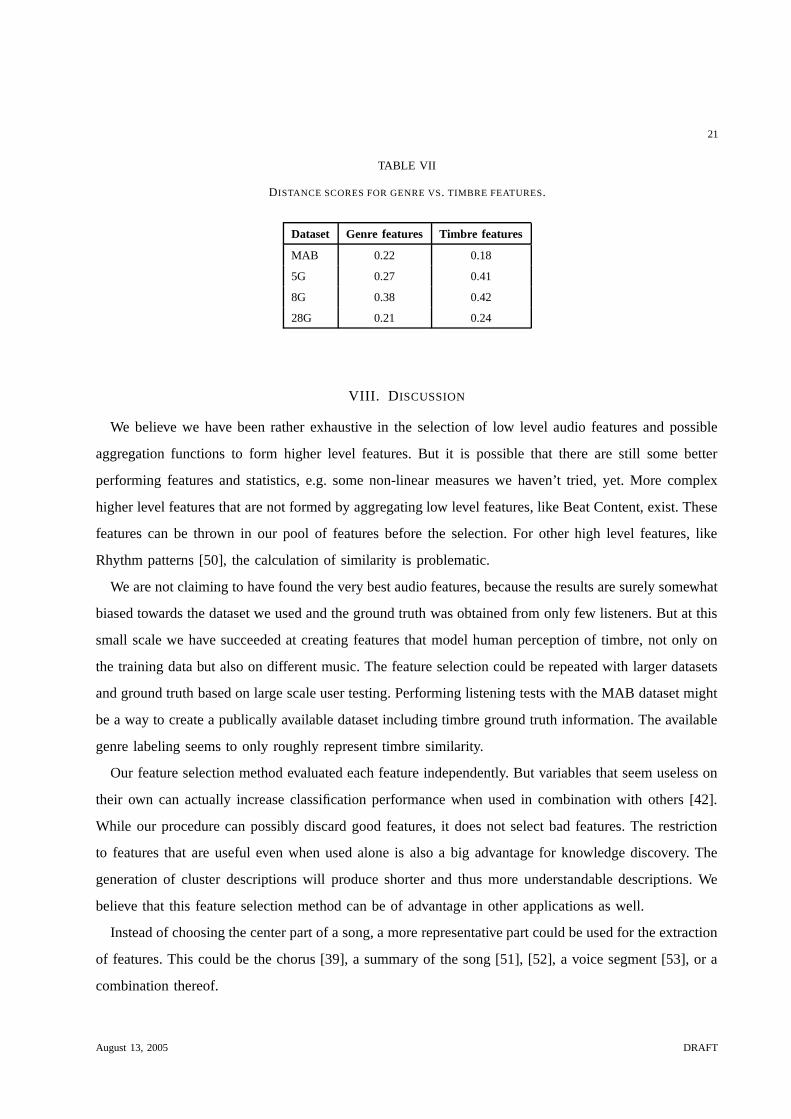
We tried to turn things around and performed the feature selection with the MAB genre data as the

training set and checked how well the top 20 features performed for timbre similarity on the 5G, 8G,

and 28G data. The results of these genre optimized features are listed in Table VII in comparison with

the results of the winning timbre features. Surprisingly, the performance of the MAB optimized features

is not much higher than for the timbre features on the very same dataset. Trying to separate genres by

intrinsic sound properties does not work as well as doing so with timbre. The performance on the 5G

data is significantly worse, because 5G was the training data for the timbre and can partly be attributed

to over fitting. The results of the genre features on the two validation datasets are both better for the

timbre features, but the margins are comparatively small. In this respect the genre categorization of the

MAB data seems to be timbre related to some degree, after all.


21

TABLE VII

DISTANCE SCORES FOR GENRE VS. TIMBRE FEATURES.

Dataset Genre features Timbre features

MAB 0.22 0.18

5G 0.27 0.41

8G 0.38 0.42

28G 0.21 0.24

VIII. DISCUSSION

We believe we have been rather exhaustive in the selection of low level audio features and possible

aggregation functions to form higher level features. But it is possible that there are still some better

performing features and statistics, e.g. some non-linear measures we haven’t tried, yet. More complex

higher level features that are not formed by aggregating low level features, like Beat Content, exist. These

features can be thrown in our pool of features before the selection. For other high level features, like

Rhythm patterns [50], the calculation of similarity is problematic.

We are not claiming to have found the very best audio features, because the results are surely somewhat

biased towards the dataset we used and the ground truth was obtained from only few listeners. But at this

small scale we have succeeded at creating features that model human perception of timbre, not only on

the training data but also on different music. The feature selection could be repeated with larger datasets

and ground truth based on large scale user testing. Performing listening tests with the MAB dataset might

be a way to create a publically available dataset including timbre ground truth information. The available

genre labeling seems to only roughly represent timbre similarity.

Our feature selection method evaluated each feature independently. But variables that seem useless on

their own can actually increase classification performance when used in combination with others [42].

While our procedure can possibly discard good features, it does not select bad features. The restriction

to features that are useful even when used alone is also a big advantage for knowledge discovery. The

generation of cluster descriptions will produce shorter and thus more understandable descriptions. We

believe that this feature selection method can be of advantage in other applications as well.

Instead of choosing the center part of a song, a more representative part could be used for the extraction

of features. This could be the chorus [39], a summary of the song [51], [52], a voice segment [53], or a

combination thereof.


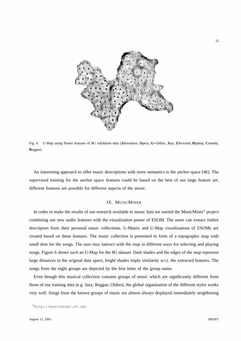
22

Fig. 6. U-Map using Pareto features of 8G validation data (Alternative, Opera, G=Oldies, Jazz, Electronic,Hiphop, Comedy,

Reggae).

An interesting approach to offer music descriptions with more semantics is the anchor space [46]. The

supervised training for the anchor space features could be based on the best of our large feature set,

different features are possible for different aspects of the music.

IX. MUSICMINER

In order to make the results of our research available to music fans we started the MusicMiner6 project

combining our new audio features with the visualization power of ESOM. The users can extract timbre

descriptors from their personal music collections. U-Matrix and U-Map visualizations of ESOMs are

created based on these features. The music collection is presented in form of a topographic map with

small dots for the songs. The user may interact with the map in different ways for selecting and playing

songs. Figure 6 shows such an U-Map for the 8G dataset. Dark shades and the edges of the map represent

large distances in the original data space, bright shades imply similarity w.r.t. the extracted features. The

songs from the eight groups are depicted by the first letter of the group name.

Even though this musical collection contains groups of music which are significantly different from

those of our training data (e.g. Jazz, Reggae, Oldies), the global organization of the different styles works

very well. Songs from the known groups of music are almost always displayed immediately neighboring

6http://musicminer.sf.net


23

each other. Cluster similarity is shown by the global topology. For example Comedy, placed in the upper

left, neighbors the Hiphop region, probably because both contain a lot of spoken (German) word. Hiphop

blends into Electronic, what can be explained by similar beats. Note, that contrary to our expectations,

there is not a complete high mountain range around each group of different music. While there is a

wall between Alternative Rock and Electronic, there is also a gate in the lower center part of the map

where these two groups blend into one another. With real life music collections this effect will be even

stronger, stressing the need for visualization that can display these relations rather than applying strict

categorizations. There is a total of five suspected outliers, most of which can be explained by a not so

well categorization of the particular songs on our behalf. This highlights the difficulties in creating a

ground truth for musical similarity, be it genre or timbre. Visualization and clustering with U-Maps can

help in detecting outliers and timbrally consistent groups of music in unlabeled datasets.

X. SUMMARY

We presented a method to select a small set of audio features for modelling timbre similarity from a

large set of possible sound descriptions. Many existing low level features were generalized. Static and

temporal statistics were consistently applied discovering the potential lurking in the behavior of low level

features over time. The quality of the resulting set of 66,000 candidate features for modelling timbre

distance was measured with novel scores based on the PDE. The winning features show low redundancy,

separate timbrally different music, and have high potential for explaining clusters of similar music. Our

music descriptors outperform seven other previously proposed feature sets on several datasets w.r.t. the

separation of the known groups of different music. The clustering and visualization capabilities of the new

features are demonstrated using U-Map displays of ESOMs . The results of the study are implemented

in the MusicMiner 7 software for the organization and exploration of personal music collections.

ACKNOWLEDGMENT

The authors would like to thank Mario N ocker, Christian Stamm, Niko Efthymiou, and Martin K ummerer

their help in the MusicMiner project.

REFERENCES

[1] G. Tzanetakis and P. Cook, “Musical genre classification of audio signals,” IEEE Transactions on Speech and Audio

Processing, vol. 10, no. 5, 2002.

7http://musicminer.sf.net


24

TABLE VIII

TOP 20 ALLROUNDER FEATURES.

Feature AR

root-pc1ps4-root-sone2 0.62

root-pc1ps2-ofcc5 0.59

mean-dstps10-mfcc1 0.58

lag1-pacf-chromaC# 0.58

lag1-pacf-mfcc33 0.56

lag3-acf-sone3 0.56

specyint-bandwidth 0.56

lag9-acf-mfcc31 0.55

std-diff2-sone19 0.54

median-diff2-chromaH 0.54

std-diff-oct-hz-centroid 0.54

nmod3-specslope 0.54

lag5-acf-bfcc14 0.53

lag7-acf-chromaH 0.53

lag5-acf-flux 0.53

std-diff2-efcc25 0.53

root-mad-diff2-melmag20 0.53

mod3-spec-sone1 0.53

lag2-acf-root-specyint 0.53

bandwidth-chromaF 0.53

[2] J. Aucouturier and F. Pachet, “Representing musical genre: a state of art,” JNMR, vol. 31, no. 1, 2003.

[3] J.-J. Aucouturier and F. Pachet, “Improving timbre similarity: How high is the sky?” Journal of Negative Results in Speech

and Audio Sciences, vol. 1, no. 1, 2004.

[4] M. McKinney and J. Breebaart, “Features for audio and music classification,” in Proceedings ISMIR 2003, 2003.

[5] E. Pampalk, A. Rauber, and D. Merkl, “Content-based organization and visualization of music archives,” in Proceedings

of the ACM Multimedia. ACM, 2002, pp. 570–579.

[6] E. Pampalk, S. Dixon, and G. Widmer, “On the evaluation of perceptual similarity measures for music,” in International

Conference on Digital Audio Effects (DAFx-03), 2003.

[7] D. Ellis, B. Whitman, A. Berenzweig, and S. Lawrence, “The quest for ground truth in musical artist similarity,” in Proc.

ISMIR-02, 2002.

[8] A. Ultsch, “Maps for the Visualization of high dimensional Data Spaces,” in Proc. WSOM’03, Japan, 2003.

[9] ——, “Self-organizing neural networks for visualization and classification,” in Proc. Conf. Soc. for Information and

Classification, Dortmund, April 1992, 1992.

[10] T. Kohonen, Self-Organizing Maps. Springer, 1995.


25

TABLE IX

TOP 20 PARETO FEATURES.

Feature PS

mean-dstps2-root-sone22 0.96

root-pc1ps4-sone2 0.95


lag3-acf-sone3 0.93

cepst1-bandwidth 0.93

lag6-acf-efcc25 0.91

mean-dstps2-efcc30 0.91


skew-angps1-chromaC# 0.89

mad-root-nchromaF# 0.89

centroid-nchromaG 0.89

std-dstps2-root-oct-centroid 0.89

lag1-acf-sone2 0.89

mod20-spec-hz-centroid 0.89

specyint-flux 0.89

cepst2-sone7 0.88

lag6-acf-flux 0.88

nmod3-spec-nchromaG# 0.88

root-mad-diff2-melmag20 0.88

cepst2-chromaF 0.88

[11] J. T. Foote, “An overview of audio information retrieval,” Multimedia Systems, vol. 7, no. 1, pp. 2–11, 1999.

[12] B. Whitman, G. Flake, and S. Lawrence, “Artist detection in music with minnowmatch,” in Proceedings of the 2001 IEEE

Workshop on Neural Networks for Signal Processing, 2001, pp. 559–568.

[13] L. Rabiner and B.-H. Juang, Fundamentals of Speech Recognition. Prentice-Hall, 1993.

[14] B. Logan and A. Salomon, “A music similarity function based on signal analysis,” in IEEE International Conference on

Multimedia and Expo, 2001, p. 190.

[15] J.-J. Aucouturier and F. Pachet, “Finding songs that sound the same,” in Proceedings of IEEE Benelux Workshop on Model

based Processing and Coding of Audio, 2002.

[16] K. West and S. Cox, “Features and classifiers for the automatic classification of musical audio signals,” in Proceedings

ISMIR 2004, 2004.

[17] J.-J. Aucouturier and F. Pachet, “Tools and architecture for the evaluation of similarity measures: case study of timbre

similarity,” in Proceedings ISMIR 2004, 2004.

[18] G. Tzanetakis, G. Essl, and P. Cook, “Automatic musical genre classification of audio signals,” in Proceedings ISMIR

2001, 2001, pp. 205–210.


26

[19] ——, “Human perception and computer extraction of beat strength,” in Proceedings Conference on Digital Audio Effects

(DAFX), 2002.

[20] G. Tzanetakis, A. Ermolinskyi, and P. Cook, “Pitch histograms in audio and symbolic music information retrieval,” in

Proceedings ISMIR 2002, 2002.

[21] T. Li, M. Ogihara, and Q. Li, “A comparative study on content-based music genre classification,” in Proceedings 26th

ACM SIGIR. ACM Press, 2003, pp. 282–289.

[22] C. Xu, N. Maddage, and X. Shao, “Musical genre classification using support vector machines,” in Proceedings of IEEE

ICASSP03, 2003, pp. V429–V432.

[23] I. Mierswa and K. Morik, “Automatic feature extraction for classifying audio data,” Machine Learning Journal, vol. 58,

pp. 127–149, 2005.

[24] F. Pachet and A. Zils, “Evolving automatically high-level music descriptors from acoustic signals,” in LNCS, 2771.

Springer, 2003.

[25] G. Tzanetakis, A. Ermolinskyi, and P. Cook, “Beyond the query-by-example paradigm: New query interfaces for music,”

in Proceedings Int. Computer Music Conference (ICMC), Gothenburg, Sweden September 2002, 2002.

[26] A. Ultsch, “Self organizing neural networks perform different from statistical k-means clustering,” in Proc. Conf. Soc. for

Information and Classification, Basel, 1995, 1995.

[27] E. Pampalk, A. Rauber, and D. Merkl, “Using smoothed data histograms for cluster visualization in self-organizing maps,”

in Proceedings of the International Conference on Artifical Neural Networks (ICANN’02). Springer, 2002.

[28] A. Ultsch, “Pareto Density Estimation: Probability Density Estimation for Knowledge Discovery,” in Proc. GfKl 2003,

Cottbus, Germany, 2003.

[29] E. Pampalk, S. Dixon, and G. Widmer, “Exploring music collections by browsing different views,” in 4th International

Conference on Music Information Retrieval (ISMIR 2003), 2003, pp. 201–208.

[30] C. C. Aggarwal, A. Hinneburg, and D. A. Keim, “On the surprising behavior of distance metrics in high dimensional

space,” Lecture Notes in Computer Science, vol. 1973, p. 420, 2001.

[31] D. Bainbridge, S. J. Cunningham, and J. S. Downie, “Visual collaging of music in a digital library,” in Proceedings ISMIR

2004, 2004.

[32] M. Torrens, P. Hertzog, and J. L. Arcos, “Visualizing and exploring personal music libraries,” in Proceedings ISMIR 2004,

2004.

[33] F. Vignoli, R. van Gulik, and H. van de Wetering, “Mapping music in the palm of your hand, explore and discover your

collection,” in Proceedings ISMIR 2004, 2004.

[34] F. M orchen, A. Ultsch, M. Thies, I. L ohken, M. N ocker, C. Stamm, N. Efthymiou, and M. K ummerer, “MusicMiner:

Visualizing timbre distances of music as topograpical maps,” Dept. of Mathematics and Computer Science, University of

Marburg, Germany, Tech. Rep., 2005.

[35] E. Zwicker and S. Stevens, “Critical bandwidths in loudness summation,” The Journal of the Acoustical Society of America,

vol. 29, no. 5, pp. 548–557, 1957.

[36] B. Moore and B. Glasberg, “A revision of Zwickers loudness model,” ACTA Acustica, vol. 82, pp. 335–345, 1996.

[37] D. Li, I. Sethi, N. Dimitrova, and T. McGee, “Classification of general audio data for content-based retrieval,” Pattern

Recognition Letters, vol. 22, pp. 533–544, 2001.

[38] N. S. Jayant and P. Noll, Digital Coding of Waveforms: Principles and Applications to Speech and Video. Prentice Hall,

1984.


27

[39] M. Goto, “A chorus-section detecting method for musical audio signals,” in Proceedings ICASSP 2003, 2003, pp. 437–440.

[40] F. Takens, “Dynamical systems and turbulencs,” in Lecture Notes in Mathematics, D. Rand and L. Young, Eds. Springer,

1981, vol. 898, pp. 366–381.

[41] A. Lindgren, M. T. Johnson, and R. J. Povinelli, “Joint frequency domain and reconstructed phase space features for speech

recognition,” in International Conference on Acoustics, Speech and Signal Processing 2004 (ICASSP04), 2004.

[42] I. Guyon and A. Elisseeff, “An introduction to variable and feature selection,” JMLR, vol. 3, no. Mar, pp. 1157–1182,

2003.

[43] P. Mitra, C. Murthy, and S. Pal, “Unsupervised feature selection using feature similarity,” IEEE Transactions on Pattern

Analysis and Machine Intelligence, vol. 24, no. 3, pp. 301–312, 2002.

[44] J. Dy and C. Brodley, “Feature selection for unsupervised learning,” JMLR, vol. 5, no. Aug, pp. 845–889, 2004.

[45] E. L. Lehmann and H. J. M. D’Abrera, Nonparametrics: Statistical Methods Based on Ranks. Prentice-Hall, 1998.

[46] A. Berenzweig, D. Ellis, and S. Lawrence, “Anchor space for classification and similarity measurement of music,” in

Proceedings ICME-03, 2003, pp. I–29–32.

[47] G. Tzanetakis and P. Cook, “MARSYAS: A framework for audio analysis,” Organised Sound, vol. 4, no. 30, 2000.

[48] E. Pampalk, “A Matlab Toolbox to compute music similarity from audio,” in 5th International Conference on Music

Information Retrieval (ISMIR 2004), 2004.

[49] O. Ritthoff, R. Klinkenberg, S. Fischer, I. Mierswa, and S. Felske, “Yale: Yet another machine learning environment,” in

LLWA 01, Dortmund, Germany, R. Klinkenberg, S. Rping, A. Fick, N. Henze, C. Herzog, R. Molitor, and O. Schrder,

Eds., 2001, pp. 84–92.

[50] S. Dixon, F. Gouyon, and G. Widmer, “Towards characterisation of music via rhythmic patterns,” in Proceedings ISMIR

2004, 2004.

[51] M. Cooper and J. Foote, “Automatic music summarization via similarity analysis,” in Proc. Third International Symposium

on Musical Information Retrieval (ISMIR), 2002.

[52] X. Shao, C. Xu, Y. Wang, and M. S. Kankanhalli, “Automatic music summarization in compressed domain,” in IEEE

International Conf. on Acoustics, Speech, and Signal Processing (ICASSP04), 2004.

[53] A. Berenzweig, D. Ellis, and S. Lawrence, “Using voice segments to improve artist classification of music,” in Proceedings

AES-22 Intl. Conf. on Virt., Synth., and Ent. Audio., 2002.

Fabian Morchen received the MS in Mathematics from the University of Wisconsin Milwaukee in 2002

and is currently writing a Ph.D. thesis on knowledge discovery from multivariate time series. He is a

member of the Data Bionics Research Group at the Philipps-University Marburg, Germany.


28

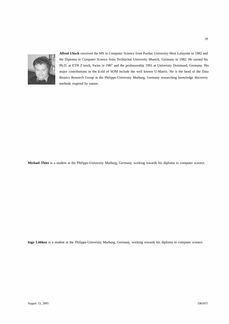
Alfred Ultsch reiceived the MS in Computer Science from Purdue University West Lafayette in 1982 and

the Diploma in Computer Science from Technichal University Munich, Germany in 1982. He earned his

Ph.D. at ETH Z urich, Swiss in 1987 and the professorship 1991 at University Dortmund, Germany. His

major contributions in the field of SOM include the well known U-Matrix. He is the head of the Data

Bionics Research Group at the Philipps-University Marburg, Germany researching knowledge discovery

methods inspired by nature.

Michael Thies is a student at the Philipps-University Marburg, Germany, working towards his diploma in computer science.

Ingo Lohken is a student at the Philipps-University Marburg, Germany, working towards his diploma in computer science.


Documents

2 Modelling timbre distance with temporal statistics from