2 Model-Based Design of a New Lightweight Aircraft Finalwpage.unina.it/agodemar/DSV-DQV/Model_Based_Design... · Model-Based Design of a New Light-weight Aircraft Arkadiy Turevskiy1,

American Institute of Aeronautics and Astronautics

1

Model-Based Design of a New Light-weight Aircraft

Arkadiy Turevskiy1, Stacey Gage2, and Craig Buhr3 The MathWorks, Inc. Natick, MA, 01760

This paper uses a combination of free and commercial off-the-shelf (COTS) modeling and simulation software to simplify and accelerate the flight vehicle design process. Using an example of a new light-weight aircraft the paper shows how a vehicle’s geometry can be optimized, stability and control coefficients calculated, open-loop plant model created, flight controller designed, and closed-loop simulation run, all in a rapid iterative fashion, to confirm that system level requirements are satisfied.

Nomenclature Cl = lift coefficient Cm = pitching moment coefficient Θ = aircraft pitch angle

I. Introduction REATING a new or modifying an existing flight vehicle is a complex and time-consuming process. Engineers have to make decisions about vehicle configuration and flight control design that will ensure that system-level

specifications are met. Any changes to hardware are very expensive and time consuming. Therefore it is important to finalize and verify the design as much as possible before any hardware is built. Model-Based Design enables engineers to test and verify their ideas in the early stages of the design process when making changes to the design is still relatively easy and inexpensive.

In this paper we use an example of a design of a new light aircraft to present a method for rapid iteration over vehicle geometric configuration and flight control design. The paper describes the steps that stability and control engineers typically go through in the early stages of the design process. These steps include: definition of the vehicle’s geometry, determination of the vehicle’s aerodynamic characteristics, creation of a simulation to verify the performance, and design of flight control laws.

Each of these steps can be a time-consuming task. In this paper we present tools and techniques for streamlining these steps and ensuring rapid iteration over the design. We first talk about a method for determining the vehicle’s aerodynamic characteristics based on its geometry. We discuss US Air Force Digital Data Compendium (Datcom) software and present results of Digital Datcom analysis of our particular vehicle configuration. We then demonstrate how to rapidly and easily import results obtained from Digital Datcom into MATLAB® for further analysis. We illustrate what preliminary analysis of aerodynamic stability and control coefficients and derivatives can reveal about the vehicle’s performance and stability.

We then show how to quickly create a simulation of a flight vehicle. We discuss modeling equations of motion, calculating forces and moments acting on the aircraft, modeling vehicle components such as sensors and actuators, and modeling environmental effects such as atmosphere, gravity, and wind gusts. We demonstrate how aerodynamic coefficients from Digital Datcom can be used in the simulation to rapidly calculate aerodynamic forces and moments acting on the vehicle.

Next, flight control design techniques are discussed. Using the example of longitudinal control design for our aircraft we show how the simulation model can be easily linearized and how a controller can be designed that meets both time domain and frequency domain specifications. We also show how, for our specific example of longitudinal flight control, we design the inner- and outer-loop controller effectively.

1 Technical Marketing Manager, 3 Apple Hill Drive, Natick, MA, 01760, AIAA member. 2 Principle Software Engineer, 3 Apple Hill Drive, Natick, MA, 01760, AIAA member. 3 Senior Developer, Control System Toolbox, 3 Apple Hill Drive, Natick, MA, 01760.

C


2

We close by discussing how the results of closed loop nonlinear simulation can be used to verify that system level requirements have been met. We also discuss how simulation results can be visualized in a high-fidelity, three-dimensional environment for detecting anomalies in flight vehicle behavior.

II. Establishing System Level Requirements Every new aircraft project or existing aircraft

modification starts with system level requirements. Examples of system level requirements include maximum take-off weight, range, level cruise speed, stall speed, maximum altitude, rate of climb, and a multitude of other specifications. System level requirements drive the design decisions and serve as the ultimate criteria for judging whether the design was successful. For the purposes of this article, we assume that our design requirements called for a light-weight four-seat monoplane with a certain level cruise speed, a certain maximum take-off weight, and a certain altitude ceiling. A more detailed description of the aircraft and system level requirements is available in Ref. 1. Figure 1 shows the general configuration of the aircraft to be designed. For simplicity purposes, in this paper we will specifically address only one requirement, namely the rate of climb for the aircraft. We will design our aircraft so that its rate of climb should be greater than or equal to 2 meters/second at an altitude of 2,000 meters above sea level.

III. Determining Vehicle Geometry Once system level specifications are available, engineers need to determine an aircraft geometry that will result

in aircraft performance that meets requirements. Aerodynamic stability and control coefficients and derivatives2 are a set of numbers that are used in aircraft equations of motion for calculating aerodynamic forces and moments acting on the aircraft. These numbers are determined by aircraft geometry and directly affect aircraft performance. Experienced control engineers have a good understanding of what these numbers need to be in order to meet system level requirements. Therefore, engineers need a method that would provide values of aerodynamic stability and control coefficients and derivatives for a given aircraft geometry. Using this method engineers can determine how to change the aircraft geometry to achieve the desired aerodynamic characteristics and, therefore, aircraft performance.

Several methods exist for determining an aircraft’s aerodynamic characteristics. The most accurate method is to measure aerodynamic forces and moments acting on the aircraft during flight testing. This method is very expensive as it requires building a flight-worthy prototype and flying it. Another method is wind tunnel testing. This method is also expensive as it requires building a wind tunnel model of an aircraft and running a wind tunnel to measure aerodynamic forces and moments acting on the model. Both wind tunnel testing and flight testing must be run at some point in the development process. Ideally, by this point, engineers already have an aircraft geometry that results in performance that meets requirements, or almost meets requirements. This minimizes the number of iterations that have to be run through wind tunnel testing and flight testing, and therefore minimizes cost. To be able to determine reasonable aircraft geometry prior to wind tunnel testing and flight testing, engineers use methods for analytical prediction of aerodynamic characteristics.

Several analytical prediction methods exist3-5. One of better known analytical methods is Digital Datcom software developed by U.S. Air Force6. This public domain software takes an aircraft geometry described in a certain input format. As the sample Digital Datcom input file in Fig. 2 shows, this file defines geometric characteristics and characteristic dimensions of an aircraft’s fuselage, wings, horizontal, and vertical tail. A detailed description of the information that needs to be specified in Digital Datcom input files can be found in Digital Datcom manual.

Figure 1. The light-weight four-seat monoplane to be designed1.


3

Figure 2. A Digital Datcom input file specifies aircraft geometry and flight conditions for the analysis.

Figure 3. A section of Digital Datcom output file shows some of the output results for the first flight condition.


4

The file shown in Fig. 2 also defines the flight conditions for which stability and control coefficients and derivatives are to be estimated. This file specifies that 320 flight conditions will be analyzed corresponding to four different values of Mach number, eight different values of altitude, and ten different values of angle of attack.

Once the input file is created, Digital Datcom can be run to produce the output file containing estimated stability and control coefficients and derivatives for the specified aircraft geometry and flight conditions. Figure 3 shows a section of Digital Datcom output file created for the input file shown in Fig. 2. The file shown in Fig. 3 is 3,180 lines long. This file is composed of 320 similar sections, each of them containing the values of the same stability and control coefficients and derivatives for each of the specified 320 flight conditions. After estimates of stability and control coefficients and derivatives are obtained, an engineer will want to have easy access to these numbers for analysis and for further use in modeling flight vehicle dynamics and control system design. As Fig. 3 shows the text format of Digital Datcom output file and its sheer size make it difficult to use for such an analysis. MATLAB®7 is a widely used commercial off-the-shelf software product that has extensive capabilities in the areas of data analysis, visualization, and reporting. Moreover, add-on products extend MATLAB capabilities in many areas - dynamic system simulation and control design being just two of them. Therefore, it would be highly desirable to have access to the Digital Datcom stability and control coefficients and derivatives in MATLAB. Aerospace Toolbox8 provides this capability by importing Digital Datcom output files into MATLAB data structures. Figure 4 shows how the datcomimport function of Aerospace Toolbox imports two Digital Datcom

output files, astdatcom1.out and astdatcom2.out into a 1-by-2 cell array of data structures in MATLAB. Each data structure in this cell array corresponds to one of the imported Digital Datcom output files and contains the values of all aerodynamic characteristics from the corresponding Digital Datcom output file, as shown in Fig 4. In this example, the lift coefficient, Cl variable in MATLAB workspace is a 10-by-4-by-8 array. The dimensions of the

Figure 4. Several Digital Datcom output files can be imported into MATLAB simultaneously usingAerospace Toolbox.


5

array correspond to the number of flight conditions defined in the Digital Datcom input file: ten angles of attack, four Mach numbers, and eight altitudes.

With all the stability and control coefficients and derivatives available in MATLAB, various plots can be quickly constructed to evaluate the performance characteristics of the aircraft. For example, Fig. 5a shows a drag polar plot

for two considered aircraft geometries corresponding to the two Digital Datcom output files imported into MATLAB. Figure 5b shows the values of pitching moment coefficient, Cm as a function of angle of attack for these two aircraft geometries. Both plots are for the flight condition of 0.1 Mach number and 5,000 feet altitude. These types of plots immediately convey useful information about the efficiency of the chosen geometry or about the effects of changes in the aircraft’s geometry on its longitudinal static stability.

IV. Creating an Open-Loop Plant Model Availability of stability and control coefficients and derivatives in MATLAB simplifies preliminary analysis

of these numbers. However, a control system has to be designed and closed-loop vehicle simulation has to be performed to understand whether the chosen vehicle geometry can lead to a vehicle design that will satisfy system level requirements. An open-loop plant model is required to start control system design. At least two approaches can be used to create the open-loop plant model.

With the first approach one would develop a linear state-space system describing the aircraft’s linearized dynamics. Stability and control coefficients and derivatives imported from Digital Datcom can be used to calculate the coefficients of state-space matrices. The resulting linear model can then be used for control design tasks. The problem with this approach is that it does not provide a control engineer with a nonlinear aircraft model that could be used for checking control design across multiple flight conditions and for determining if the vehicle’s performance satisfies system level requirements. Therefore, an alternative approach is proposed.

With the alternative approach, an open-loop plant model is constructed using full nonlinear equations of motion. The open-loop model developed this way can be linearized at a specific flight condition for control design, and can also be later used for nonlinear closed-loop simulation to determine if the chosen aircraft geometry and flight control design result in aircraft performance that meets system level requirements.

In the first step of this approach, an open loop model is constructed with equations of motion, based on Newton’s second law. These equations of motion are solved by integrating input forces and moments to find aircraft’s position and attitude. A convenient way to organize these calculations is through the use of Simulink®9. With this product an engineer can choose the appropriate blocks from the Simulink block library, place them into the model, and connect them. Aerospace Blockset10 contains a library of blocks implementing equations of motions. A block from that library could be used as a starting point for the open-loop model. A library of blocks implementing six degrees-of-freedom (DOF) equations of motion is shown in Fig. 6. In the case of this article, a three-DOF (Body Axes) block was chosen and placed into a Simulink model for modeling the longitudinal dynamics of the aircraft.

a) Drag polar plot. b) Pitching moment coefficient. Figure 5. Digital Datcom coefficients can be used for preliminary configuration analysis in MATLAB.


6

This block can be replaced with a six-DOF equations of motion block at a later time when the dynamic model is further elaborated. Forces and moments that are inputs to the equations of motion come from several different sources: gravity, propulsion, and aerodynamics (aeroelastic effects are not considered in this article, but can be added later for higher fidelity simulation).

To calculate gravity forces and moments, a local gravity vector has to be multiplied by vehicle mass and converted to wind axes. For calculating propulsion forces and moments, a simple lookup table was used to calculate thrust as a function of throttle command, and the propulsive moment was assumed equal to zero. Calculation of gravity and propulsive forces and moments is shown in Fig. 7 (in this figure and all subsequent figures blocks from

Figure 6. Equations of motion can be implemented with one of the blocks from the Aerospace Blockset Equations of Motion library.

a) Calculation of gravity force. b) Calculation of propulsive forces and moments. Figure 7. Forces and moments acting on the aircraft include gravity force and propulsive forces andmoments.


7

Aerospace Blockset are highlighted in blue). In accordance with Model-Based Design, these calculations can be further elaborated when a more precise dynamic model of the vehicle is required.

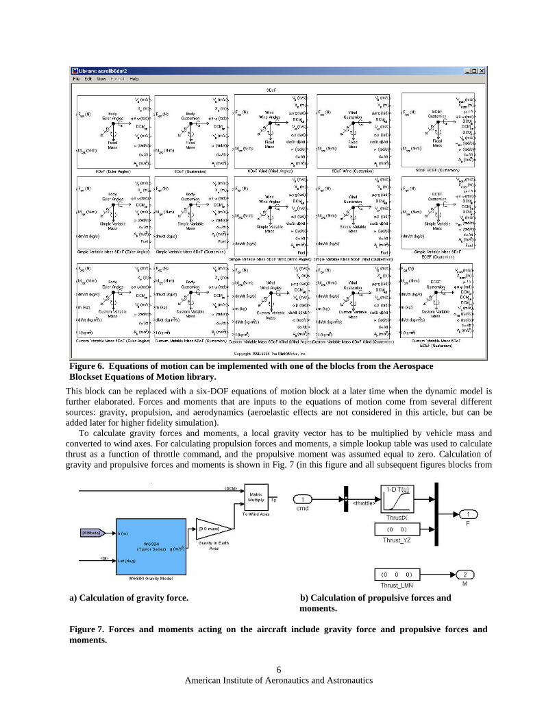
Aerospace Blockset provides a Digital Datcom Forces and Moments block that calculates static and dynamic aerodynamic forces and moments acting on the aircraft using stability and control coefficients and derivatives

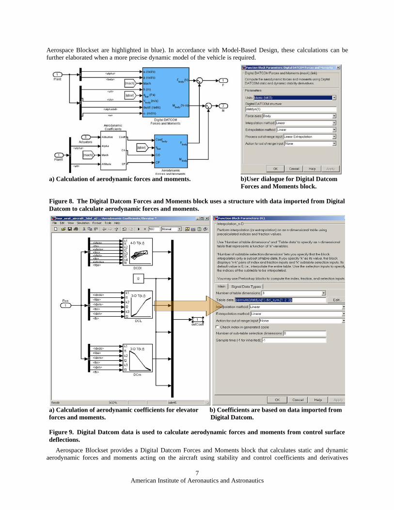
a) Calculation of aerodynamic coefficients for elevator b) Coefficients are based on data imported fromforces and moments. Digital Datcom. Figure 9. Digital Datcom data is used to calculate aerodynamic forces and moments from control surfacedeflections.

a) Calculation of aerodynamic forces and moments. b)User dialogue for Digital Datcom Forces and Moments block. Figure 8. The Digital Datcom Forces and Moments block uses a structure with data imported from Digital Datcom to calculate aerodynamic forces and moments.


8

imported from a Digital Datcom output file. In addition to the Digital Datcom Forces and Moments block, another calculation is needed to determine short-term aerodynamic forces and moments created by control surface deflections. Figure 8a shows how the Digital Datcom Forces and Moments block is used to calculate static and dynamic aerodynamic forces and moments. Figure 8b shows the user dialog for the Digital Datcom Forces and Moments block. Figure 8a also shows the calculation of total aerodynamic forces and moments, which is achieved by adding static and dynamic aerodynamic forces and moments calculated by the Digital Datcom Forces and Moments block with forces and moments created by the aircraft’s control surface deflections (calculated in Aerodynamic Forces and Moments subsystem in Fig. 8a). Figure 8b shows that the name of the MATLAB structure containing Digital Datcom stability and control coefficients and derivatives is specified in the user dialog for the Digital Datcom Forces and Moments block in the Digital Datcom structure field. Aerodynamic coefficients used for calculating forces and moments created by control surface deflections are also based on stability and control derivatives imported from Digital Datcom. For example, Fig. 9 shows the calculation of coefficients for determining aerodynamic forces and moments generated by elevator deflection. Once a Simulink model for the open- loop plant model has been setup, it can be quickly updated for different aircraft geometries by simply importing a new Digital Datcom output file containing the aerodynamic characteristics for the new geometry. The vehicle’s mass and inertia properties may need to be updated as well.

The open-loop plant model to be used for control design should also include actuator models as well as sensor dynamics. Blocks from Aerospace Blockset were used for this purpose. Figure 10 shows a subsystem implementing

Figure 10. Actuator dynamics were modeled with Aerospace Blockset blocks.

a) Wind turbulence model. b) Model of the atmosphere.

Figure 11. Model fidelity was increased by including environmental effects.


9

actuator dynamics. Aerospace Blockset blocks were also used to increase the fidelity of the model by adding environmental effects.

Specifically, wind turbulence models from Aerospace Blockset were used to calculate wind velocities as shown in Fig. 11a. The Committee on Extension to International Standard Atmosphere (COESA) model was used to model changes in atmospheric temperature, pressure, density, and local speed of sound as shown in Fig. 11b. These values were used for calculating Mach number and dynamic pressure values.

Finally, to keep calculations consistent, transformations from body axes to inertial axes, from wind axes to body axes, and from vehicle coordinates in the inertial coordinate system to vehicle latitude, longitude, and altitude had to be performed. All these operations were done using the appropriate block from Aerospace Blockset.

V. Designing Flight Control System For the purposes of this article, a longitudinal flight controller for the aircraft was developed. With the open-

loop nonlinear model created, the next steps are to select the control architecture and linearize the model for linear control design. Simulink® Control Design11 made this convenient by providing the ability to apply the linear control design tools directly on the Simulink model by specifying the blocks in the model to tune and specifying closed loop input and output signals with linearization points. The first step is to modify the open-loop system with the control architecture to close the loop. This is done by inserting blocks into the model that represent flight control logic. In the discussed example, the longitudinal controller represents a two-loop setup, shown in Fig. 12. An inner loop uses

the measurement of pitch angle, θ, and the outer loop uses the measurement of the aircraft’s altitude. The structure of the longitudinal controller in Simulink is shown in Fig. 13. The output linearization point, measured altitude, is also shown in Fig. 13. The input linearization point is altitude command.

With input and output linearization points specified and the controllers for both the inner loop and the outer loop specified as the blocks to tune, as shown in Fig. 14a, Simulink Control Design automatically linearizes the plant about the default operating point. A different operating point can be specified, as was done in this example, by specifying a certain simulation time. The state of the system at the specified time will be used as the operating point for linearization. In the specific example discussed here, the operating point was calculated at a simulation time of five seconds, when the system was in steady state. In addition, Simulink Control Design automatically defines feedback loops to be used in the design, as shown in Fig. 14b. The next step of the process was to specify design and analysis plots. In this case root locus charts were used for design and a step response plot was used for analysis.

Figure 12. Longitudinal controller consists of an inner pitch loop and an outer altitude loop.

Figure 13. Longitudinal controller in Simulink also consists of inner pitch loop and outer altitude loop.


10

With Simulink Control Design setup completed, the tool could be used for interactive graphical tuning of the controller. Effects of changes in the controller’s gains or pole and zero locations, as shown in Fig. 15a, can be immediately observed in the analysis plots as shown in Fig. 15b.

Because the control system in the case of a longitudinal controller includes inner and outer loops, any changes to the inner loop compensator affect the outer loop dynamics, and any changes to the outer loop compensator influence inner loop dynamics. This is shown schematically in Fig. 12. This interdependency makes tuning of two control loops more difficult.

a) Selecting blocks to tune. b) Loop naming. Figure 14. Simulink Control Design was used to select blocks to tune and to name the loops.

a) Loop gains as well as pole and zero locations can b) The step response updates as changes are made. be changed. Figure 15. Controller was tuned interactively using graphical tuning.

Figure 16. The outer loop was “broken” to simplify loop tuning.


11

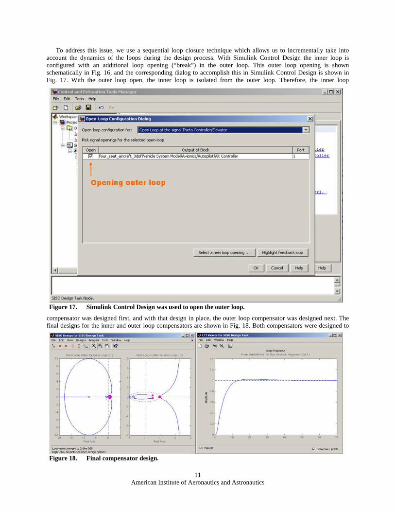
To address this issue, we use a sequential loop closure technique which allows us to incrementally take into account the dynamics of the loops during the design process. With Simulink Control Design the inner loop is configured with an additional loop opening (“break”) in the outer loop. This outer loop opening is shown schematically in Fig. 16, and the corresponding dialog to accomplish this in Simulink Control Design is shown in Fig. 17. With the outer loop open, the inner loop is isolated from the outer loop. Therefore, the inner loop

compensator was designed first, and with that design in place, the outer loop compensator was designed next. The final designs for the inner and outer loop compensators are shown in Fig. 18. Both compensators were designed to

Figure 17. Simulink Control Design was used to open the outer loop.

Figure 18. Final compensator design.


12

provide a satisfactory step response and to satisfy the frequency domain requirements of 9dB gain margin as well as 30 degrees phase margin for the inner loop and 65 degree phase margin for the outer loop. As we only considered climb rate requirement at 2,000 meters for this article, the longitudinal flight controller was designed solely around the operating point corresponding to the trim condition at this altitude. To design a flight controller for the whole flight envelope, multiple operating points could be chosen corresponding to various flight conditions spanning the flight envelope, and multiple compensators could be designed, with one compensator for each operating point. Simulink Control Design supports this workflow.

A flight controller over the whole flight envelop could then be implemented by gain scheduling the designed compensators with flight conditions such as Mach number and altitude.

VI. Simulating Nonlinear Closed-Loop Dynamics Once the flight controller has been designed, full nonlinear closed-loop simulation could be performed to verify

compensator performance in a nonlinear model and to check if the aircraft design met system level requirements. Once the detailed open-loop plant model was developed, as descried in section IV, and the closed loop system with preliminary compensator design was set up, as described in section V, all that needed to be done was to update compensator coefficients in the appropriate Simulink blocks with the values from the final compensator design. Simulink Control Design enables easy updates of compensator coefficients with the Update Simulink Blocks Parameters button, as shown in Fig. 19.

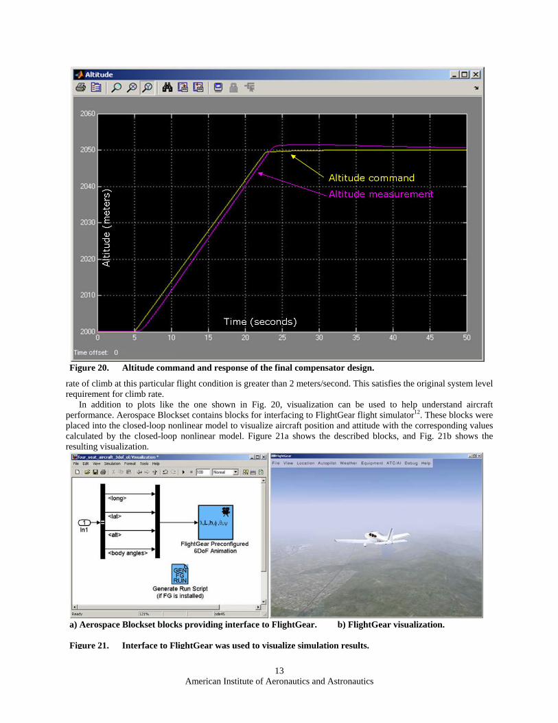
Closed-loop simulation was run by commanding a change of altitude from 2,000 meters to 2,050 meters starting at 5 seconds of simulation time. The altitude command and altitude response are shown in Fig. 20, which demonstrates that the longitudinal flight controller provides a stable response. It can also be seen that the measured altitude reaches 2,050 meters fewer than 20 seconds after the requested change in altitude. Therefore, the aircraft’s

Figure 19. Simulink model was updated with compensator values designed with Simulink ControlDesign.


13

rate of climb at this particular flight condition is greater than 2 meters/second. This satisfies the original system level requirement for climb rate.

In addition to plots like the one shown in Fig. 20, visualization can be used to help understand aircraft performance. Aerospace Blockset contains blocks for interfacing to FlightGear flight simulator12. These blocks were placed into the closed-loop nonlinear model to visualize aircraft position and attitude with the corresponding values calculated by the closed-loop nonlinear model. Figure 21a shows the described blocks, and Fig. 21b shows the resulting visualization.

Figure 20. Altitude command and response of the final compensator design.

a) Aerospace Blockset blocks providing interface to FlightGear. b) FlightGear visualization.

Figure 21. Interface to FlightGear was used to visualize simulation results.


14

VII. Iterating over the Controller and Aircraft Design In the somewhat simple example described in this article, the closed-loop system met system level requirements.

More realistically, it can be expected that multiple design iterations will be needed. Further, different types of iterations could be needed.

The design of the controller could be iterated on. For example, if desired the climb rate was not achieved, a better control design could be tried to achieve a faster rise time. Closed-loop simulation could then be rerun to determine if the revised controller design meets system level requirements. It could, however, be determined that the best possible control design still results in a failure to meet system level requirements for a given aircraft configuration. Therefore, iteration on the aircraft’s geometric configuration might be needed as well.

In the considered example, if the climb rate requirement was not met, designers could investigate a different wing shape or a larger wing area to make the aircraft climb faster. The changes in geometry would naturally affect other areas of performance for the aircraft. These changes would have to be investigated to ensure that meeting one system level requirement does not result in violating other requirements.

The described design process does not eliminate the need for multiple design iterations. It does, however, provide a way to go thorough design iterations faster and more efficiently.

VIII. Conclusions An aircraft design process using both free and commercial off-the-shelf software products has been proposed.

Using an example of a new light-weight monoplane, it was shown how aircraft aerodynamic characteristics can be quickly estimated and analyzed. It was also shown how an open-loop aircraft model can be quickly created using pre-built blocks and using control and stability coefficients and derivatives derived from the aircraft’s geometric configuration. It was shown how to linearize the plant and how to design a flight control system. It was shown how the open-loop plant model can be augmented with control logic to create a closed-loop nonlinear model which can be used for both control design and validation. The process of designing a flight control system using linear control design techniques for the closed-loop model was demonstrated. It was also shown how simulations of the nonlinear model can be used for checking the controller’s performance and for determining if system level requirements have been met. The proposed design process allows for quick iterations through aircraft geometric configurations and control design. With this approach designers can create aircraft geometry that will meet system level requirements by using software tools rather than by building the actual prototypes. The simulation models developed with the proposed approach can be easily elaborated and updated with experimental data from wind tunnel testing or actual flight tests.

References 1 Cannon, M., Gabbard, M., Meyer, T., Morrison, S., Skocik, M., Woods, D., "Swineworks D-200 Sky Hogg Design

Proposal," AIAA/General Dynamics Corporation Team Aircraft Design Competition, 1991-1992. 2 Stevens, B., and Lewis. F., Aircraft Control and Simulation, 1st ed., John Wiley & Sons Inc., Hoboken, New Jersey, 1992,

Chap. 2. 3 Park, M., Green, L., Montgomery. R., and Raney, D., “Determination of Stability and Control Derivatives Using

Computational Fluid Dynamics and Automatic Differentiation,” NASA Technical Report NASA-AIAA-99-3136, NASA Langley Technical Report Server, 1999.

4 Green, B., and Chung, J., “CFD Predictions of the Stability and Control Characteristics of the Pre-Production F/A-18E,” AIAA Atmospheric Flight Mechanics Conference and Exhibit, San Francisco, California, 2005.

5 Moore, F., McInville, R., and Hymer, T., "Application of the 1998 Version of the Aeroprediction Code," Journal of Spacecraft and Rockets, Vol. 36, No. 5, 1999, pp.633-645.

6 Williams, J., and Vukelich, S., “The USAF Stability and Control Digital Datcom”, AFFDL-TR-79-3032, 1979. 7 MATLAB, “MATLAB User’s Guide”, The MathWorks, Inc., Natick, MA, March 2007. 8 Aerospace Toolbox, “Aerospace Toolbox User’s Guide”, The MathWorks, Inc., Natick, MA, March 2007. 9 Simulink, “Simulink User’s Guide”, The MathWorks, Inc., Natick, MA, March 2007. 10 Aerospace Blockset, “Aerospace Blockset User’s Guide”, The MathWorks, Inc., Natick, MA, March 2007. 11 Simulink, Control Design, “Simulink Control Design User’s Guide”, The MathWorks, Inc., Natick, MA, March 2007. 12 FlightGear Flight Simulator, Software Package, Ver. 0.9.10, 2007.

©1994-2007 by The MathWorks, Inc., MATLAB, Simulink, Stateflow, Handle Graphics, Real-Time Workshop, SimBiology, SimHydraulics, SimEvents, and xPC TargetBox are registered trademarks and The MathWorks, the L-shaped membrane logo, Embedded MATLAB, and PolySpace are trademarks of The MathWorks, Inc. Other product or brand names are trademarks or registered trademarks of their respective holders.


15

Documents

2 Model-Based Design of a New Lightweight Aircraft Finalwpage.unina.it/agodemar/DSV-DQV/Model_Based_Design... · Model-Based Design of a New Light-weight Aircraft Arkadiy Turevskiy1,