AALTO UNIVERSITY

School of Engineering

Department of Engineering Design and Production

Teemu Halmeaho

Magnetic bearing as switched reluctance motor

Thesis submitted in partial fulfillment of the requirements for the degree of

Master of Science in Technology

Espoo August 7 2012

Supervisor Professor Petri Kuosmanen

Instructor Kari Tammi DSc (Tech)

AALTO UNIVERSITY SCHOOLS OF TECHNOLOGY PO Box 11000 FI-00076 AALTO httpwwwaaltofi

ABSTRACT OF THE MASTERrsquoS THESIS

Author Teemu Halmeaho

Title Magnetic bearing as Switched Reluctance Motor

School School of Engineering

Department Department of Engineering Design and Production

Professorship Machine Design Code Kon-41

Supervisor Professor Petri Kuosmanen

Instructor Kari Tammi DSc (Tech)

Abstract The goal of this work was to research the similarities between active magnetic bearings and switched reluctance motor and particularly research the chances for converting magnetic bearing into switched reluctance motor In addition ways to cope with the widely reported problems the motor type has were studied The test environment consisted of test rig previously used for testing control methods for magnetic bearing In addition to this MATLAB Simulink simulation models were built to help the designing of the test setup The test setup had two alternative controllers an original magnetic bearing controller modified to work as a motor controller and a new CompactRIO-based controller that was used for comparing different speed control and commutation methods New rotor designs were engineered to work with the prototype motor that used unmodified magnetic bearing stator This setup was tested for obtaining the output torque and maximum speed of the motor together with the accuracy to follow set values Test results of simulations and test setup were inside the error margins showing the use of simulations beneficial in design process of this type of a motor The tests revealed differences between the control methods suggesting using the advanced angle controller and adjustable commutation angles

Date 782012 Language English Number of pages 86 + 12

Keywords magnetic bearing reluctance motor speed control machine design simulation

AALTO-YLIOPISTO PL 11000 00076 AALTO httpwwwaaltofi

DIPLOMITYOumlN TIIVISTELMAuml

Tekijauml Teemu Halmeaho

Tyoumln nimi Aktiivinen magneettilaakeri vaihtoreluktanssimoottorina

Korkeakoulu Insinoumloumlritieteiden korkeakoulu

Laitos Koneenrakennustekniikan laitos

Professuuri Koneensuunnitteluoppi Koodi Kon-41

Tyoumln valvoja Professori Petri Kuosmanen

Tyoumln ohjaaja Tekniikan tohtori Kari Tammi

Tiivistelmauml

Tyoumln tavoitteena oli tutkia yhtenevaumlisyyksiauml aktiivimagneettilaakerien ja vaihtoreluktanssimoottorin vaumllillauml Tutkimus keskittyi erityisesti arvioimaan mahdollisuuksia muuntaa magneettilaakeri vaihtoreluktanssimoottoriksi Lisaumlksi tutkittiin keinoja ratkaista ongelmia joita taumlmaumln tyyppisessauml saumlhkoumlmoottorissa on raportoitu olevan Testiympaumlristouml koostui roottorikoelaitteesta jota on aikaisemmin kaumlytetty magneettilaakerin saumlaumltoumljaumlrjestelmaumln tutkimuksessa Lisaumlksi rakennettiin MATLAB Simulink simulointimalli jota kaumlytettiin moottorin saumlaumltoumljaumlrjestelmaumln suunnittelun apuna Testilaitteessa oli kaksi vaihtoehtoista saumlaumltoumljaumlrjestelmaumlauml alkuperaumlinen magneettilaakerin ohjain muokattuna toimimaan moottorin ohjaimena sekauml uusi CompactRIO -jaumlrjestelmaumlaumln perustuva saumlaumltoumljaumlrjestelmauml Jaumllkimmaumlistauml kaumlytettiin erilaisten nopeus- ja kommutointitapojen vertailuun keskenaumlaumln Prototyyppimoottorin staattori oli sama jota kaumlytettiin magneettilaakerin kanssa Roottori suunniteltiin sopimaan juuri taumlhaumln kaumlyttoumltarkoitukseen Taumltauml koelaitetta testattiin vaumlaumlntoumlmomentin ja maksiminopeuden selvittaumlmiseksi Lisaumlksi suoritettiin testejauml joissa tutkittiin kykyauml seurata nopeuden asetusarvoa Simuloimalla saadut tulokset olivat hyvin laumlhellauml koelaitteella saatuja tuloksia osoittaen simuloinnin kaumlytoumln olevan hyoumldyllistauml taumlmaumln tyyppisen moottorin suunnittelussa Saumlaumltoumlmenetelmaumlt suoriutuivat vaihtelevalla menestyksellauml testeistauml Suositeltava saumlaumltoumlmenetelmauml oli edistyskulman saumlaumldin joka kaumlytti hyvaumlkseen saumlaumldettaumlviauml kommutointikulmia

Paumlivaumlmaumlaumlrauml 782012 Kieli englanti Sivumaumlaumlrauml 86 + 12

Avainsanat magneettilaakeri reluktanssimoottori nopeussaumlaumltouml koneensuunnittelu simulointi

Foreword The work in this Masterrsquos Thesis was carried out at VTT Technical Research Centre of Finland Industrial Systems in Electrical Product Concepts team of Smart Machines knowledge center I wish to thank former Technology Manager of smart machines Pekka Koskinen for giving me the chance to work at VTT in the first place I am also grateful to current Technology Manager Johannes Hyrynen for giving me the opportunity to carry on working in this great team I wish to thank Professor Petri Kuosmanen the supervisor of this thesis and Res Prof Tammi the instructor of the thesis I greatly appreciate the wisdom of both of you I would like to express my gratitude towards MSc (Tech) Tuomas Haarnoja who co-instructed this work with Res Prof Tammi In addition to this he had notable contribution on FEM modeling part of this work together with the design and manufacturing of an electrical converter circuit needed in this work I wish to thank also Mr Timo Lindroos for milling the rotor parts despite his busy schedule I also thank other colleagues who helped me during this work I wish to thank my family and friends specially my parents-in-law Dr Kirsi-Marja Oksman-Caldentey and Dr Javier Caldentey for sharing me their scientific perspective of life and giving guidance throughout this work The most of everyone I wish to thank my beautiful wife Tania for standing by me not just during this thesis but also for the whole time of my studentship For my ten months old son Nico I am grateful for tearing only a few pages of the drafts

Espoo 782012 Teemu Halmeaho

Table of Contents

Abstract Tiivistelmauml Foreword Nomenclature

1 Introduction 1

11 Background 1

12 Research problems 3

13 Aim of the research 3

14 Limitations 4

15 Methods of research 4

16 Own contribution 5

2 Magnetic bearings and Switched Reluctance Motor 6

21 Magnetic bearings 6

22 Electric motors in general 8

23 SRM compared to other electric motors 11

24 Physical characteristics behind SRM 13

3 State of the art 17

31 Research on SRM 17

32 Control theory for basic SRM operation 19

321 Mathematical model 20

322 Power electronics and controller 26

33 Solutions for problems with SRM 30

331 Torque ripple 30

332 Radial vibration 31

333 Noise 33

334 Bearingless SRM 34

4 Materials amp methods 37

41 Test environment 37

411 Simulations of the model 39

412 Test setups 40

42 Test planning 45

421 Rotor designs 45

422 Steps of the tests 46

43 Estimations for error 49

431 Error in mathematical methods 49

432 Error in test setup 49

5 Results 51

51 Deceleration measurements to obtain resistance torque 51

52 Acceleration measurements to obtain torque values 51

521 Acceleration from 240 rpm to 420 rpm using the AMB controller 52

522 Acceleration from 0 rpm to 250 rpm using different control methods in the cRIO 54

523 Acceleration from 240 rpm to 420 rpm using different control methods in the cRIO 57

524 Acceleration in simulations 59

53 Step and sweep response measurements 63

531 Sweep response with AMB 63

532 Step response with cRIO 65

54 Maximum speeds 69

541 Using AMB 69

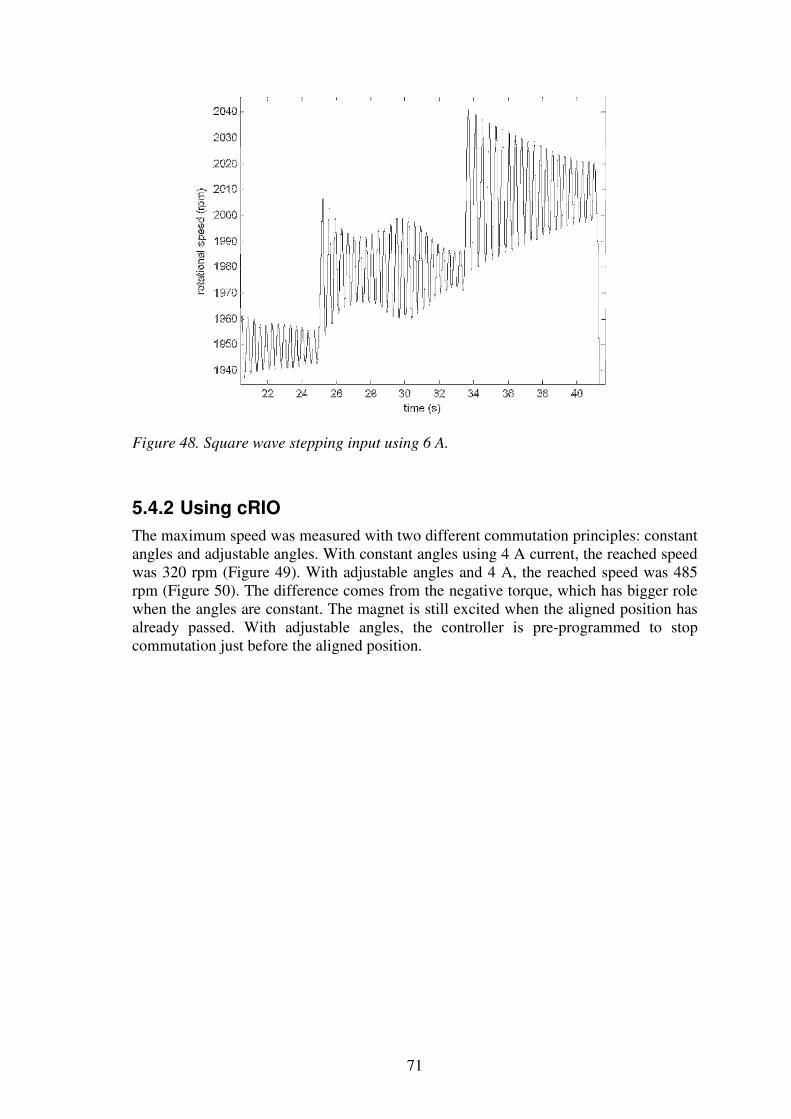
542 Using cRIO 71

6 Discussion 73

61 Conclusions from test results 73

62 Applications for SRM 76

63 Future work 77

7 Summary 79

References 81

Appendices

Appendix A Specific Simulink model

Appendix B Simplified Simulink model Appendix C Simulink model converted to LabVIEW Appendix D Real-time part of the LabVIEW VI used for controlling the SRM Appendix E FPGA part of the LabVIEW VI used for controlling the SRM Appendix F Error budget for pure mathematical model error Appendix G Error budget for difference between the simulation model and the test setup

Nomenclature

Abbreviations AALZ Advanced Angle controller using the Linearized motor model AAAL Advanced Angle controller Assuming Linear behavior of the motor AMB Active Magnetic Bearing AC Alternating Current AVC Active Vibration Control BEV Battery Electric Vehicle BLDC Brushless Direct Current Motor BSRM Bearingless Switched Reluctance Motor CCAA Current Controller using Adjustable Angles CCCA Current Controller using Constant Angles cRIO Compact Reconfigurable Input Output DC Direct Current FEM Finite Element Method FPGA Field Programmable Gate Array HEV Hydrogen Electric Vehicle MBS Multi Body Simulation PWM Pulse-Width Modulation SRM Switched Reluctance Motor

Symbols

θ Rotational angle

θoff Ending angle of commutation θon Starting angle of commutation θm Advanced angle micro0 Permeability of air ω Rotational speed B Flux density F Force f Frequency

I i Current L Inductance La Inductance when rotor and stator poles are aligned Lu Inductance when rotor and stator poles are un aligned m Number of phases n Rotational speed Np Number of rotations in coil Npar Number of coils connected in parallel

Nr Number of rotor poles Nser Number of coils connected in series Pin Input power Pout Output power p Number of magnetic pole pairs T Nominal torque Tavg Average torque Tpeak Maximum torque

Wmotor Energy supplied for motor V Voltage W Energy transformed into mechanical energy

1

1 Introduction

11 Background

The use of magnetic bearings (here referred to as active magnetic bearings abbreviated AMBs) in rotating machines brings advantages compared to traditional bearings AMBs use an active magnetic force control to levitate rotor inside stator leaving an air gap between the rotor and the stator They have some good inherent properties such as low friction (Nordmann amp Aenis 2004) possibility to control and monitor the rotor movement (Schweitzer 2002) almost maintenance-free operation and stability at high speeds (Matsumura et al 1997) These good qualities can be found also in switched reluctance motors (SRMs) since their working principles are similar In addition there are other good electric motor qualities in SRMs such as low production costs (Cao et al 2009) through ease of manufacture (Cameron et al 1992) with plain stator construction and robust rotor structure (Li et al 2009) SRM is an electric motor where both rotor and stator have salient structure When simplified this means both of them having poles The stator poles are wound forming coils The rotor is a simpler part It does not have any windings on it The material used in the rotor is soft iron being passive component compared to for example brushless direct current motor which has permanent magnets in the rotor When the opposite stator coils are excited the rotor tends to move to a position where the reluctance is least and therefore the magnetic flux passing through the rotor is at maximum When the next adjacent stator coil pair is activated the rotor rotates to the next aligned position to minimize the air gap between the active poles of the stator and the rotor The switching frequency between adjacent coils determines the rotation speed of the motor More generally the speed n is defined by the switching frequency f between the magnetic pole pairs p

(1)

The switching is done electronically using the feedback information of the rotor angle to correctly do the timing of the on and off switching of the coils A stator of an AMB resembles the one in the SRM The rotor is as simple as it can be imagined a cylindrical rod The working principle to produce radial force with the AMB is also based on activating the coils to generate the magnetic flux that pierces the rotor Depending on the layout of the poles in the stator the flux can go all the way to the opposite half of the rotor when the difference of magnetic fluxes in opposite sides of the rotor defines the magnitude of the radial force This happens only if at least two separate opposite magnets are in active at the same time The magnetic flux can alternatively penetrate slightly when only one magnet instead of two is excited In both cases the radial force is produced

2

The history of SRMs goes more than hundred years back This is because it has close relation to synchronous reluctance motor step motor and inductance motor at least it had in 19th century Nowadays they do not have that much in common except their electromagnetic similarities They all have power control methods of their own and their structures are different (Toliyat amp Kliman 2004) The current form of SRM started to shape in the 1960s and continued to develop up to the 1980s Fundamental problems were found and solutions suggested (Cai 2004) The main problems in implementing these solutions were the lack of computation power and sufficiently good electronics In addition not all of the flaws were found at that time because of the limitations of measuring technology Due to advances in computer science control engineering and electronics since the late 1990s it has been possible to cope with the awkward nature of SRMs However even today SRMs have not got that much of usage as a power source Although some applications have been around since the early years of SRM it has not skyrocketed at any time The most recent application has been in the vacuum-machine industry In the near future however there may be an opportunity for low cost electric motors such as the SRM The trend in the price of permanent magnets has been upward for some time which hikes up the material costs of many other competing electric motor types The interest on the subject of this masterrsquos thesis aroused from the fact that SRMs can become increasingly popular in a short time The work was done at VTTrsquos Electrical Product Concepts team where AMBs have been researched before (Tammi 2007) Tammi (2007) focused on studying a control system for the radial vibration attenuation of the rotating shaft The test arrangements involved a test rig which was also used as a base for this study In practice only minor physical modifications are needed for converting a magnetic bearing into a motor Replacing the cylindrical rotor with a branched one and using a slightly different control method should get the rotation started Nevertheless to make it behave properly a little more is needed The nonlinear character of the SRM produces torque ripple (Cai 2004) The nonlinearity is a result of doubly-salient structure where magnetic flux is a function of the angular position of the rotor In addition acoustic noise is generated by the vibration of the stator The vibration is born from the radial forces acting between the rotor and the stator (Wu amp Pollock 1995) The aerodynamic resistance is the other reason for the acoustic noise The balance in loudness between these two noise sources depends on the construction of the motor Usually the stator vibration is the dominant one The stator vibration can be forced or born when system excited with the natural frequency of the system Another radial vibration problem is the movement of the rotor shaft This movement can be also divided into forced and natural frequency of the system-originated vibration All these issues mentioned will be under discussion during the whole work The most interesting design for SRM is the one where the bearing function is combined with the motor function This hybrid system can be achieved by using two separate stators or by combining both functions in one stator In practice the latter alternative needs a more complex stator design or at least a more sophisticated control algorithm (Takemoto et al 2001) The ultimate engineering goal for making a good SRM-driven mechanical system would be to build this kind of hybrid system that outputs smooth torque with a properly attenuated stator vibrations combined to shaft movement

3

attenuation In addition traditional mechanical bearings could be replaced or at least reduced to one

12 Research problems

As an outcome of this section a scope for the research is formed The bottom question was whether it is possible to convert an AMB to SRM simply by replacing the rotor and updating the control algorithm As mentioned earlier the nonlinear nature is a major source for most of the problems SRM has This is why even the simplest motor functions and their design process can be considered as a challenge Modeling of SRMrsquos operation precise enough to give an approximation of its performance was under the lens In addition one problem was how difficult it is in practice to implement a closed-loop system to control the rotation speed of the physical system Answers to these questions are given as extensive way as possible The other SRM problems are torque ripple and radial vibrations The vibration in the stator also evokes acoustic noise The main source for the vibration is the radial force between the rotor and stator (Cameron et al 1992) In addition the air resistance of the rotor poles produces some noise (Fiedler et al 2005) A literature review is given to enlighten the possible ways to cope with these three In this research prospects for the multifunctional hybrid SRM system that can include vibration attenuation with bearing function in addition to motor function is considered The main purpose of this research was to gain knowledge on SRM This was reasonable because generally engineers do not know this type of electric motors In addition the ones who know it have a bit negative attitude against them and it has been reported that even misleading claims are made in research papers (Miller 2002) This is because SRM needs a more modern approach compared to the other electric motors It has issues that need mechanical- control- computer - and electrical engineering skills to be understood and solved Depending on the issue a different skill is needed but to understand the relations between them an engineer needs at least some experience in all of the mentioned fields

13 Aim of the research

As said the aim of the research was to gain knowledge on SRM The more precise actions were namely to get an understanding how to solve most of the problems of SRM simulating SRM operation resurrecting the previously used AMB test device and converting the AMB into SRM At first it was researched if the rotor has any rotation at all using the modified AMB control system With the original AMB controller the rotor rotates in a magnetic field without any feedback from the angular position After successfully completing this a new control system with both hardware and software is put up to replace the old one With this a closed loop commutation is implemented using the feedback information of the angular position measurements In addition two different speed control methods are implemented One being traditional current-limiting PI controller and another more sophisticated including also a high-resolution commutation method to optimize the controllability of SRM

4

14 Limitations

About the boundary conditions that affect reaching the goals of the research is discussed next Two main factors were limiting this research Firstly the scope of the Masterrsquos Thesis in general was actually quite narrow for researching something that is not well known in engineering society Especially in this case where multi-disciplinary knowledge is needed as discussed earlier there will be a lot of groundwork to be done Secondly the stator of the original magnetic bearing test device could not be modified because it was an original prototype of a previous AMB study Considering these limitations several aspects are worth discussing In the stator there were Hall sensors sticking out in every pole and a safety plate bearing protecting the sensors from having physical contact with the rotor The construction was not very compact which meant that there was a rather large air gap between the stator and the rotor Most probably this is dramatically reducing the output torque of the motor Although the safety plate may come in use if something goes wrong Another thing considering the stator was the coupling of the poles There were eight poles connected as adjacent pairs forming four magnets This defined the number of rotor poles to be two The scope of Masterrsquos Thesis gave mainly a limit for the time resources available This affected to the research problems that were chosen to be part of this particular research Not all of the SRM flaws were possible to include to the scope in same scale as the others In practice this meant finding an answer to some of the SRM problems only in a form of a literature review

15 Methods of research

This section presents actions making it possible to reach the goals in the environment where previously mentioned boundary conditions stand The research can be divided into three phases which were executed partially in parallel to support each other Still the preceding phases worked as a foundation for the subsequent tasks The starting point was theoretical approach that produced a mathematical model to describe the behavior of SRM In addition there is given an insight into methods to cope with the other SRM problems than just the ones that are faced with commutation and speed control In the second phase based on the mathematical model a simulation model was created using MATLAB Simulink This model is converted into LabVIEW simulation model to be later modified into LabVIEW real-time control system The final phase was the physical test setup This began with tests using the original AMB controller Later the test setup is updated to work with controller that consists of LabVIEW and CompactRIO (cRIO) a reconfigurable embedded control and monitoring system Another purpose for simulations was to get a better understanding of SRM especially how to control it and to get a more specific estimate of its performance capabilities If it is possible to build accurate enough model it can be used to estimate what actions should be done to increase the performance of the SRM in the test setup Simulation results are also an interesting point of comparison The main research method was the physical test setup As explained earlier the test rig used to be a test environment for magnetic bearing This made it convenient for SRM usage Due to restrictions that did not allow modifying the stator the motor type was

5

defined to be a 2-phase 42 motor which means that there are two different states during one revolution and four poles in the stator and two poles in the rotor This type of SRM is one of the simplest constructions there are so it suited well for basic testing With the test setup a series of tests were performed In tests the focus was on performance analysis In addition to 42 type motor an 86 (eight stator poles and six rotor poles) was also inspected when theoretical aspects were considered This was because 86 is a 4-phase motor which brought some interesting aspects when control strategies were considered

16 Own contribution

Everything mentioned in the work was entirely done by the author except the design and manufacturing of an SRM inverter FEM models and manufacturing of the rotors The scientific contribution this work has to offer is firstly the corrections done for the method expressing the SRM torque presented by (Li et al 2009) This was proven right by unit comparison In addition after the editing the results started to agree with other methods to calculate the SRM torque Secondly built-in MATLAB Simulink block describing the dynamics of SRM was corrected to output speed in the same units the block description stated This was proven using authorrsquos own Simulink model to describe the equation of the motion which was the faulty part of the block Thirdly it was verified experimentally that eight-pole AMB stator does not convert into eight-pole SRM stator to be used together with six-pole rotor converting the AMB to 86 SRM Instead the eight-pole AMB stator was verified to convert into four-pole SRM stator forming a 42 SRM

6

2 Magnetic bearings and Switched Reluctance Motor

21 Magnetic bearings

In this section the history of magnetic bearings and working principles are enlightened The concept of a magnetic bearing is actually more recent than that of SRMrsquos The reason for this might be that the advantages compared to traditional bearings were not needed in any way before because there were other non-ideal components involved When thinking of the original version of the magnetic bearing a passive magnetic bearing not so many benefits can actually be found Before any actual concepts of magnetic bearings were introduced it was shown that stable levitation using permanent magnets is not possible in free space where all three rotational and transitional degrees of freedom should be covered by the magnets (Earnshaw 1842) The first approaches to design a magnetic bearing were in the 1930s and the studies at that time were more or less theoretical It was only in the 1980s when the active magnetic bearing studies begun intensively Before that the lack of good enough electronic components and computers were limiting the research enthusiasm In the 1990s the state of the art was in the level where the commercial products could be launched (Matsumura et al 1997) (Schweitzer amp Maslen 2009) The first applications were in the area of turbo-machinery and it remains as a main area of usage Other popular applications are for example machine tools medical devices and different kind of pumps In general magnetic bearings can fit well in applications that have either high rotation speed or demanding operation environment There are also three special ways of using AMBs bearingless motor unbalance control and self-diagnosing smart machine Some of the applications mentioned may be using these techniques as a part of their operation These techniques can be seen as intelligent ways of using the active magnetic bearings (Matsumura et al 1997) (Schweitzer amp Maslen 2009) The term bearingless motor is widely used but actually it is a self-bearing motor This kind of motor has rotor and stator constructions where the motoring and bearing functions are combined The setup where a torque producing stator and another stator that produces supporting forces are distinct is not considered as a self-bearing motor Although if the stator is constructed to be only one actuator with separate windings but the rotor has two portions of different geometries it can be classified as self-bearing The key in here is the compact structure In fact the latter example has suffered in compactness compared to ideal case where the motoring winding can be used also for the bearing function and separate rotor portions are not needed The ideal case has a performance problem because the rotor and stator constructions are trade-offs between the output torque and the support capacity of the bearing There is also an advanced way to support the shaft by the means of unbalance control The key is to keep the eccentricity of the shaft rotation in minimum in addition for supporting the rotor against the gravity The self-bearing motor can be constructed to include the unbalance control also Induction motors controlling the eccentricity have been studied in (Laiho et al 2009) and (Laiho et al 2011) With self-diagnosing smart machine the unexpected system changes can be found before any severe malfunctions For example

7

the bearing can detect if the force needed to support the shaft is increased significantly which can be a sign of a sudden failure of some component in the system The three special techniques mentioned have self-explanatory benefits Other properties that make AMBs desirable to certain use are contactless operation rotor can be run fast without losing its balance low bearing losses adjustable dynamics and low maintenance costs with high life time (Schweitzer amp Maslen 2009) The operation principle of the active magnetic bearing can be described as contactless support of the shaft In addition to support AMB suspends and guides the rod (Chiba et al 2005) The actuator is normally constructed so that there are magnets in four perpendicular directions forming orthogonal coordinate system This way it is possible to produce both positive and negative force in each direction separately Electromagnet is composed of two adjacent wounded poles that are connected in series forming a horseshoe magnet (Figure 1) This way the total number of poles is eight Each magnet is independent of each other therefore four force components can be operated separately The higher the number of poles gets more costs will be born This is why a three pole AMB has been studied by (Chen amp Hsu 2002) The control system Chen amp Hsu used was more complex than what is needed with eight-pole version The simplest AMB control method uses only one magnet to produce one pulling force component Hence if a force component pointing straight up would be needed as it is the case in situation of Figure 1 only the upmost horseshoe magnet would be activated The excited magnet produces a pulling force that tries to minimize the length of the air gap According to (Schweitzer 2002) the radial force of Figure 1 produced by one horseshoe magnet is defined as 1413 cos (2)

Here micro0 is the permeability of air n is the number of rotations in one coil 13 is the cross-

sectional area of the coil is the winding current s is the air gap length and is the glancing angle of the pole While the air gap decreases the pulling force increases

causing non-linear behavior as seen from the equation (2) where the air gap length is inversely quadratic The feedback measurements of the air gap length are provided for the controller to calculate the forces to minimize the unwanted deflection (Chiba et al 2005) In addition the current also causes non-linear control behavior This is why sometimes AMBs are controlled using opposite magnet pairs If both of the magnets are fed with the same current they should produce opposite force components with equal magnitude both trying to pull the rotor away from the center point The resultant force is zero but if the control current of one of these two magnets is raised above the preload bias current the resultant force will point towards the magnet excited with higher current The Fi plot should be linearized around suitable operating point to provide longest possible operation range Hence value of the bias current will be the start of the linearized slope

8

Figure 1Illustrative figure of one horseshoe magnet of AMB pulling the rotor

22 Electric motors in general

A short review of different electric motor types is given in this chapter There is more than just one way to divide electric motors into different categories Here the division is done by distinguishing different commutation methods As a result four categories for electric motors were formed The main reason for using this kind of method was the demand to find a category also for SRM The method was adapted from (Yeadon amp Yeadon 2001) The four compartments are direct current motors alternating current induction motors synchronous machines and electronically commutated motors The latter is the one that includes the SRM Most of the divisions used in handbooks do not include SRM at all it is rather described as a special type of an electric motor This review was done especially from the motor control and commutation point of view The commutation is needed to pass the current to the rotor and to change the direction of rotation Normally the change of direction is done at every 180 mechanical degrees to maintain the torque production during one revolution The review can be seen useful because the SRM is not well known and it makes a point to compare it to more widely used electric motors to estimate its potential uses The brushed direct-current motor is considered as the simplest electric motor from the control-engineering point of view It has a linear speed-voltage ratio and torque-current ratio The stator consists of permanent or electromagnets forming field wiring that is fed with direct current The armature winding is located on the rotor The commutator feeds alternating current for the armature winding The commutation is managed via brushes that have a tendency to sparkle and wear out during time The biggest problem with the brushed DC motor is the frequent need for maintenance concerning the brushes To solve this problem a brushless DC motor (BLDC) has been developed This motor type

9

will be described with the electronically commutated motors (Toliyat amp Kliman 2004) (Yeadon amp Yeadon 2001) The AC induction motor is the most popular electric motor at least in the industrial -use some say it is the most used in home and business also It has wound stator poles to produce magnetomotive force that causes torque The rotor has a squirrel cage structure that is used for catching the current induced by the rotating magnetic field produced on stator windings This way a torque-producing magnetic field is formed in the rotor Induction motors can be broken down to single-phase and polyphase motors Single-phase motor uses single-phase power and poly-phase motors use multiphase usually three-phase power The latter is usually available only in industrial sites This is why in home and business the induction motors are normally single-phase type In single-phase motor the rotating magnetic field is not born unlike in its multiphase brother To produce the rotating field there are multiple methods depending on the application where the single-phase motor is used The difference between these methods is how they get the rotation started In the applications that do not require high starting torque a shading coil can be used In this method a time lag is produced in the flux that passes through the shading coil causing an initial rotating magnetic field This field is enough to start rotating the rotor When the rotor speeds up the main rotating magnetic field is produced by the rotor Another version of single-phase motor is a split-phase induction motor Common version of this type is to use a capacitor in series together with a startup winding which is separate from the main winding This method provides higher starting torque than the shading coil method (Toliyat amp Kliman 2004) (Yeadon amp Yeadon 2001) Synchronous machines have a lot in common with induction motors Although in synchronous motors the phase between the magnetic fields of the rotor and the stator is synchronous in induction motors the fields are not in the same phase but the inducting field is leading the induced field by the slip factor describing the tendency to have phase difference This is why induction machines are also known as asynchronous machines Three synchronous motor working principles can be found to be distinct from each other reluctance hysteresis and permanent magnet All of these have stator construction that is almost identical with the induction motor stator Different rotor types define different working principles The synchronous reluctance motor has a damper winding in the rotor to help with starting the motor if used in direct on-line The winding is adapted from the induction motor and the motor actually works as an induction motor until the synchronous speed is reached When the motor runs at synchronous speed the pole winding is being exploited Alternative way for direct on-line is to use frequency converter that enables to run the motor in synchronous all along from start to top speed The damper winding is no longer needed when a frequency converter is introduced The second category in synchronous motors is hysteresis motors The key in hysteresis motor is the rotor that is manufactured from such steel which has hysteresis properties to make the magnetization lag behind the applied field It is because of the phase shift between the induced magnetization in the rotor and the magnetic field in the stator that makes the motor to start In time the rotor catches up the stator field and the phase shift goes to zero making the motor run at synchronous speed Again the pole winding is excited to keep up the synchronous speed The third

10

version permanent magnet synchronous machine resembles the brushless DC machine They both have permanent magnets inside the rotor and an electronically controlled stator Although the BLDC uses electronic commutation more than just to get the rotation started Another way to start up the motor is to use unevenly distributed stator poles with a return spring These kind of unidirectional motors are suitable only for modest applications In synchronous speed the magnets lock into the rotating magnetic field produced in the stator All the synchronous motor types mentioned so far are so called non-excited machines There are also DC-excited machines that use slip rings and brushes to carry the current for the rotor (Toliyat amp Kliman 2004) (Yeadon amp Yeadon 2001) The most interesting and challenging group of motors in control engineering point of view is the electronically commutated motors They are all DC-powered and commutated electronically instead of mechanical This group contains the brushless direct current motor the step motor and the switched reluctance motor The key to work with the electronically commutated motors is to have information of the rotation angle This information is used to trigger the magnetic fluxes on and off The angle is normally measured but in the case of step motor there is no feedback This is because with step motors the angle can be determined from the previously fed pulses In all of these three motors there can be found a clear structural consistency that is derived from the commutation method that is used the windings are located on the stator instead of the rotor This results in salient pole cross-section in the rotor (Toliyat amp Kliman 2004) (Yeadon amp Yeadon 2001) The brushless DC motor has permanent magnets inside the rotor It has linear current-to-torque and speed-to-torque relationships Compared to the traditional brushed DC motor the brushless improves some poor properties Downsides are the additional costs and complexity (Yeadon amp Yeadon 2001) Step motors come in three structures variable-reluctance permanent magnet-rotor and hybrid permanent magnet The rotation of the step motors is best described as stepping Every step is a stationary state and one revolution can be composed of more than several hundred steps The operating principle is close to SRM but the main difference is the stationary states If step motor is fed with a frequency converter trying to rotate the motor so fast that it cannot find the stationary states it loses the steps This actually reduces the speed of the motor because the following steps do not match the rotor position The same thing happens with a critical load the motor fails to produce enough torque For these reasons step motors are used only in applications that have known loads and need positioning only at moderate speed In variable reluctance step motor the toothing in the rotor and in the stator poles is dense to create many steps This way the positioning is accurate Although there are many common features in variable reluctance step motor and SRM the SRM is designed to operate in different applications The fact that SRM is lacking the dense toothing of the poles is the key difference In SRM there are no stationary states so the position angle feedback is required for the commutation In principle the positioning applications are not impossible for SRM but using it in such a way does not take the full advantage of SRMrsquos capabilities It is the non-linear character what makes the positioning difficult

11

Other electric motors can perform such task better because of the linear nature A more suitable application for SRM is in traditional electrical power to mechanical power conversion where good acceleration and high speed is needed In the following chapters detailed descriptions of the SRM working principles are presented (Toliyat amp Kliman 2004) (Yeadon amp Yeadon 2001)

23 SRM compared to other electric motors

To sum up the similarities of SRM compared to other electric motors three motor types were taken into comparison As stated earlier SRM can be thought as a special case of a variable reluctance stepper motor Actually the right way to put it would be vice versa because SRM was discovered first Nevertheless stepper motors are known more widely so it makes sense to keep them as a reference In theory the constructions are the same despite the pole toothing in some stepper motors The rotation of SRM is continuous unlike in stepper motors This means they have control methods of their own and different optimal use The relation to brushless direct current motor is the active phase-to-phase rotation of the magnetic flux at discrete rotor angles that are programmed to the controller This is true only in the case of BLDC that has square wave input The third motor type synchronous reluctance motor may sound like a close relative to SRM but has nothing to do with it In older publications a variable reluctance motor can be found This actually means SRM not the step motor and it was used confusingly especially in the United States for some period The roots of SRM are there where the first electric motors where invented The working principle is simple so it was not hard to discover the motor after the concept of electric motor in general was proposed The most significant difference between the earliest structures and todays design is in commutation method The first versions used mechanical switches instead of electrical transistors The mechanical switching produced inaccurate and slow magnetic flux switching This meant low torque and slow rotation speed The first application was to propel a locomotive in 1838 The speed was 4 miles per hour (Byrne et al 1985) Effective operation of SRM calls for fast electronics and motor controller that is configured for the specific motor setup It was in the 1960s when it was possible to use electronic components to control the SRM In practice the first controllers for actual prototypes and products were created in the 1970s and 1980s These first versions had only the necessary functionalities to use SRM as a power source with speed control The compensation of the unwanted side effects was not in interest at that time It was challenging enough to implement the fundamental functionalities using computers and software of the time At that time the design process of SRM was heavier than nowadays To verify the geometry of the rotor and the stator finite element analysis is needed Now the FEM software can be run on an ordinary PC but 30 years ago the situation was something else The commutation logic in the motor controller also needs to be simulated first to obtain the optimal angles for the wanted performance nature Because these analyses were not available when the first versions were designed engineers needed to rely on the theoretical examination In the 1990s the computer science was advanced enough to make possible deeper analyses when designing motors At that time the design process of SRM reached the point where the motor was ready to be used in many applications The only problem was that

12

it was too late The other electric motor types were already infiltrated into the industry Because those others had simpler nature it took less work to streamline the design and the engineering process The fact that SRM does not bring any significant improvements compared to competing motors makes it unwanted as a substitutive technology especially when compared to induction motor Ten years later the interest towards this motor type woke up again and at this moment is receiving considerable attention by the scientists involved with electric motors Now the interest is on compensating the unwanted side effects that is evoked by the working principle Addition to this the focus is on combining the magnetic bearing to the motor forming a bearingless motor The interest towards this motor type arises from the inherent good qualities On the other hand many not so good properties are characteristic to this motor type As mentioned earlier in the past the rivals for the SRM had shorter and faster path to commercial use as a power source The reason for this is these specific unwanted properties Some of them relate to the motor itself and others are more related to controller The most relevant pros and cons have already been analyzed or will be analyzed further in the work Therefore only summary of them is presented here in a Table 1 When analyzing the qualities in Table 1 description for optimal application for SRM can be found by combining these pros and cons The manufacturing cost structure of SRM is biased towards high initial costs because of high design expenses coming from controller that needs to be tuned for specific motor In addition this motor type is yet missing network for sub-contractor manufacturers unlike every other type electric motor On the other hand the manufacturing costs coming from materials and assembly are low Hence specific for optimal application area should be large production numbers and a natural tendency to accept the motor and the controller as a package where they are integrated together by the same manufacturer Because the rivals of the SRM have so strong status in all possible industries it makes sense to aim for newish application area that does not yet have a standard practice The most promising target is an electric vehicle SRM could be a power source both in Battery Electric Vehicle (BEV) and in Hydrogen Electric Vehicle (HEV) which are the two most vital technologies for the vehicle of the future When alternatives for the electric motor role in electric cars are reviewed there are usually at least these three contenders induction motor brushless DC-motor and SRM The SRM has an average to good success in reviews (Larminie amp Lowry 2003) (Chan 2007) (Xue et al 2008) According to (Rahman et al 2000) SRM was described having potential for performance superior to brushless DC-motors and induction motors when these three were compared for electric vehicle applications The main decrease of points seems to come from the complex control method and from the unusualness that may lead to higher costs than with induction motor At the same time the commonly mentioned positive aspects for vehicle propulsion are the first nine positive aspects listed in Table 1 The end verdict of the reviews usually states that selecting between these motor types is not the most crucial thing when designing an electric vehicle because there are also many other engineering challenges that need to be taken into account

13

Table 1 The pros and cons of SRM (Miller 1993) (Miller 2002) (Larminie amp Lowry

2003) (Takemoto et al 2001) (Rahman et al 2000)

Positive properties Negative properties

++++ Robust and rugged construction

++++ Almost maintenance free

++++ Low material costs

++++ Low manufacturing costs

++++ Good heat conductivity because windings are on the stator

++++ Low inertia allows high acceleration

++++ Efficiency can be maintained over wide range of torque and speed

++++ Possibility to operate in high temperatures

++++ Operation as generator possible

++++ Possibility to build bearingless motor

++++ High-speed operation possible

++++ No sparking tendency so usage in the explosion hazard environment possible

minusminusminusminus Torque ripple

minusminusminusminus Noise

minusminusminusminus Stator vibrations

minusminusminusminus Complex control method

minusminusminusminus Controller needs to be tuned for specific motor design

minusminusminusminus Small air gap needed

minusminusminusminus Angular position feedback required

minusminusminusminus Not well known technology

minusminusminusminus Limited sub-contractor network available

24 Physical characteristics behind SRM

Plain description of SRMrsquos nature has already been given in previous chapters Next the subject is examined more thoroughly The cross-sectional view of SRM is presented in Figure 2 Even though the figure is a conceptual drawing it actually does not differ that much from the actual appearance of SRM The real rotor geometry is exactly as it is drawn no windings or permanent magnets are present The air gap in the drawing is exaggerated the thumb rule for the air gap length is 05 of the outer diameter of the rotor (Miller 1993) Still having smaller air gap length than 025 mm may lead to mechanical problems with tolerances The reason why so small length is recommended is the low permeability of air and high permeability of iron The magnetic flux tends to choose the path that has the lowest magnetic reluctance The word reluctance occurs also in the name of SRM It means magnetic resistance and is inversely proportional to the permeability of the material If the air gap between the rotor pole and the stator pole is too long the flux does not reach out over the air gap to meet the rotor lowering the flux density The flux density is a product of current i and inductance L The rate of change in inductance related to angular position θ determines the available torque (Miller 2001) 12 (3)

14

Thus too large air gap means poor output torque Then having a smaller air gap leads to more noisy construction because of the non-uniform structure In Figure 2 the rotor is aligned with the stator coils AArsquo If the direction of rotation is anticlockwise the next coil pair to be activated is BBrsquo When BBrsquo is excited the AArsquo is turned out To get the maximum torque simultaneous coil pair activation can be used Hence before the rotor is aligned with the AArsquo the BBrsquo can be switched on to get higher torque More about the commutation strategies will be discussed later

Figure 2 Cross-section of 86 Switched Reluctance Motor

The number of poles in the rotor and in the stator defines the number of phases The ratio between these three aspects determines the basic type of the motor The simplest version of SRM is shown in Figure 3 This kind of 22 setup having two rotor and stator poles has some problems It has only one phase so the torque has extremely high ripple Most of the time coils cannot be excited to prevent the negative torque that would slow down the rotation speed In addition to poor torque the motor cannot be started in arbitrary angles because the change in inductance is zero during wide range of the resolution In practice the 4-phase 86 setup shown in Figure 2 has turned out to be the most sensible layout It was one of the first configurations used in commercial products (Miller 2002) The main problem in 2-phase motor is the lack of self-starting Performance is also lower than in 4-phase situation When using a rotor that has specially designed pole shapes the 2-phase motor can be started from any given angle but it has a downside of limiting the direction of rotation to only one direction This special rotor construction has secondary poles forming a stepping between the main pole and the secondary In chapter 421 Rotor designs is described a rotor design that utilizes the stepping to enable the arbitrary starting angle In 3-phase motors the 128 setup is sometimes used for its simpler power electronics In 3-phase motor there has to be more poles in the stator and rotor to get the same number of strokes which makes the motor more expensive In addition there may be problems with producing enough

15

torque to get the motor started in arbitrary angles The number of strokes is the product of number of phases and number of poles in the rotor So the number of strokes is equal in both 4-phase 86 and in 3-phase 128 With high stroke number the torque ripple is lower In 2-phase version the setup should be 812 to get the same number of strokes To sum up the 4-phase 86 has the advantage of self-starting capability at any position to both directions with high number of strokes achieved with low number of poles Miller (2002) has done a review of worthwhile pole and phase combinations The phase numbers of five and higher are not recommended by Miller due to increased costs in controller that need to have more channels He also told that high pole numbers should be avoided because of unsatisfactory inductance ratio

Figure 3 Cross-section of 22 SRM

The windings are connected as pairs and in Figure 2 they are signed with the same letter for example AArsquo forming one pair The opposite coils of one coil pair are switched on at the same time but usually they are connected in series to manage with fever electrical components This is the principal difference in AMB and SRM winding because with AMB the adjacent instead of opposite coils are connected together The current in excited windings generates magnetic flux in the iron core of the stator Usually this flux goes through the rotor to the opposite iron core on the other side of the stator that was also excited The flux can also just pierce the rotor pole returning to the same stator pole it left The magnetic flux can be represented with swarm of lines describing flux density like those presented in Figure 4 From the picture also the return flow of the flux in the back iron of the stator and flux in the interface between the rotor and the stator can be seen The flux is obtained from FEM-model calculations Because the coils are activated alternately the flux is not constant or even continuous between two sequential phases When more than one pole pair is exited the fluxes

16

produced by separate coils change the density and path of the flux piercing the rotor In addition during one coil pair activation the flux is also non-linear with respect to rotation angle because of the continuously changing air gap length

Figure 4 Magnetic fluxes in 86 SRM (Haarnoja 2012)

17

3 State of the art

31 Research on SRM

A short review of the past research on SRM is given in this section The review is divided into seven categories regarding the research scope The first category is a principal study such as this Masterrsquos Thesis Others are research of the torque ripple radial vibration noise bearingless switched reluctance motor sensorless control and finally applications This division categorizes extensively the papers published regarding the SRM Usually the research scope is defined to be one of these topics However some studies handle multiple issues due to close relation of issues to each other In here is referred into only part of the overall research done on a certain topic However for every research can be found at least one suchlike study on the same time As in research in general the studies can be divided into verifying assumptions and into resolving problems In the first case the research concentrates on finding relations between phenomenon and in the later figuring out methods to cope with something that does not have a general solution yet Studies from both of these categories are reviewed next The methods for resolving the SRM problems will be looked more thoroughly in chapter 33 The research of basic SRM operation concentrates mainly on describing the production of main output component of a motor torque At first is determined a mathematical model to describe the production of torque Usually this model is a mechanical model describing mechanical torque but sometimes an equivalent electrical circuit is formed leading into electromagnetic torque The basic research is either general know how or it is more concentrated on something specific basic function such as improving the power intensity of the motor This Masterrsquos thesis handles mostly commutation and speed control which is the most essential part of electric motors This topic was the first focus when electronic control of SRM was included in research The time before SRM was not controlled electronically using microprocessors is not included in this review nor was the research too intense anyway at the time One of the first papers that fulfill the scope was published by (Bose et al 1986) It was a thorough study of SRM in general which also included a working prototype of the motor This kind of basic research was in interest especially in the early 90s (Miller amp McGlip 1990) (Materu amp Krishnan 1990) (Stefanovic amp Vukosavic 1991) and ten years later when SRM was found again now as interesting subject for modern control engineering (Miller 2002) (Rfajdus et al 2004) (Chancharoensook amp Rahman 2002) (Ho et al 1998) (Chancharoensook amp Rahman 2000) (Soares amp Costa Branco 2001) (Barnes amp Pollock 1998) Even today papers are published regarding optimization using the newest methods (Jessi Sahaya Shanthi et al 2012) (Petrus et al 2011) (Hannoun et al 2011) (Pop et al 2011)

Torque ripple has been interesting as a research object since the 1990s Especially finding a solution for the ripple has been scope for many researchers The interest lasted for about ten years and it still can be found as a secondary object in many studies As a summary can be said that only a little can be done to torque ripple if decrease in performance is not acceptable Even though the lower performance can be tolerated the

18

ripple remains high It seems torque ripple has earned its place as part of SRMrsquos nature The methods for the reduction have relied mostly on control engineering (Russa et al 1998) (Mir et al 1999) (Cajander amp Le-Huy 2006) (Henriques et al 2000) although mechanical properties of the rotor have been also considered (Lee et al 2004) The radial vibration is a problem just by itself and in addition it produces acoustic noise However the noise is treated as an individual problem in here The radial vibration is same kind of principal problem of SRM as is the torque ripple This is why the vibration was also an interesting matter at the same time in the 1990s To reduce the vibration level different approaches has been suggested First ways used at the 90s were to affect to power control of SRM by controlling transistor switching in an intelligent way (Wu amp Pollock 1995) This method has been research subject recently in (Liu et al 2010) Another way to cope with vibrations is to use mechanical means and more precisely by using optimal stator construction This has been under investigation by (Cai et al 2003) and (Li et al 2009) The most popular radial vibration attenuation subject has been to operate with bearingless SRM The BSRM combines functionality of an active magnetic bearing with the SRMrsquos motor function This way it is possible to cancel the vibration before it is even actually born The acoustic noise is usually an indication of vibration Thus if the vibration can be attenuated the noise should also decrease This is true if the noise source is entirely vibration born not aerodynamic as it sometimes is Many researches that have set topic on finding solution for noise in SRM are concentrating on finding a way to cope with the vibration (Wu amp Pollock 1995) (Cameron et al 1992) This is why the noise topic has gathered interest at the same time as the vibration studies In (Fiedler et al 2005) was shown aerodynamic noise to be the dominant source in some cases Fiedler et al (2005) proposed solutions for aerodynamic problems that were simple when compared to what is needed to solve problems in radial vibration Bearingless SRM can be used for solving the radial vibration problem which may also generate noise First studies that also included prototypes were published in the start of 21st century (Takemoto et al 2001) Today this remains as the most interesting subject when SRM is considered Many studies are approaching BSRM by using separate coils for radial force and motoring (Takemoto et al 2001) (Cao et al 2009) (Guan et al 2011) but it is also possible to use simpler construction (Chen amp Hofmann 2010) (Morrison et al 2008) The advantage of using this kind of simpler topology is the lower costs in manufacturing It seems that there are different ways to implement the BSRM and it is likely that not all the ways are yet researched One trend in SRM is to design sensorless motors These types of motors are not using any external probes or such to produce feedback information of the system This kind of setup is reasonable because the sensors are expensive (Bass et al 1987) the motor suffers in compactness with them (Cheok amp Ertugrul 2000) and there is an increased chance of malfunction when sensors are used (Ray amp Al-Bahadly 1993) The simplest way for sensorless operation is to forget the closed loop control and feed the stator with square wave signal that corresponds the motor phases The problem is how to make sure

19

the rotor does not fall out from the phase and catches the rotating magnetic field at start up When the first attempts were made in the end of 1980s the sensorless action was implemented in this way but complemented with current measurements from the some point of the power electronics circuit (Bass et al 1987) This kind of method was still researched ten years later although with more sophisticated usage of the feedback current information (Gallegos-Lopez et al 1998) In 1993 the state of the art in sensorless control of SRM was reviewed and the verdict was that none of the techniques of the time was good enough to be used in actual products (Ray amp Al-Bahadly 1993) Since that the trend has been more towards fuzzy control (Cheok amp Ertugrul 2000) and neural networks (Mese amp Torry 2002) (Hudson et al 2008) where the angular position is deduced from measured current or flux In addition specific analytical models are also used which may lead into extremely heavy computing requirements (Hongwei et al 2004) Hongwei et al (2004) calculated the feedback information from the rate of change in measured inductance A more recent review of the sensorless methods is given by (Ehsani amp Fahimi 2002) stating the techniques are now on a level that is more implementable But then again if SRMs are manufactured in means of mass production the variation in parameters that are used in sensorless methods are so high that self-tuning controller needs to be used In addition Ehsani amp Fahimi (2002) pointed out that these parameters are used also with normal SRMs This said the self-tuning should be used regardless of the feedback method In practice this would mean using neural networks in every controller designed for any given SRM especially since aging of materials also affect into these parameters The final category is the applications SRM is not mentioned in many studies where alternatives for something certain application are reviewed However electric and hybrid cars are one common interest amongst researchers when applications for SRM are considered Alternatives for electrical propulsion motor are reviewed in both (Chan 2007) and (Xue et al 2008) The approach is only theoretical but they both suggest SRM over other types of electric motors In addition tests that are more specific were done for prototype of SRM attached on actual car by (Rahman et al 2000) Rahman states that SRM produces better performance than brushless direct current motor or induction motor when used as a power source of a car In reviews for electric car motors these two motor types are included in most cases together with permanent magnet motors Another SRM included automotive application is a combined starter and generator The reason for popularity in car related subjects is clear when thinking of SRMrsquos robust and almost maintenance free construction In research done by (Cai 2004) SRM had only moderate success but SRM was analyzed based on out dated information

32 Control theory for basic SRM operation

Different ways to design the mathematical model power electronics and control algorithms of SRM are shown in the following sub sections First the mathematical models to calculate the most essential outputs and internal parameters are discussed Second some basic knowledge of power electronics used in SRMs is described Third commutation and how to control the rotation speed of SRM are explained Usually a type of mathematical model of SRM is required to design a controller A basic

20

controller takes care of the commutation of SRM More advanced controller algorithms include pulse shaping to optimize for instance the torque ripple or the noise and vibrations emitted The control algorithms are usually realized in a digital electronics controlling the driving power electronics

321 Mathematical model

From the system point of view the primary output of a motor can be considered torque Caused by the torque a motor starts to rotate the shaft at specific acceleration dependent on the inertia of the system together with the motor torque and resistive torques Hence when these are known the acceleration can be calculated This is why it is important to have an accurate model to estimate the motor torque Due to the non-linear nature of SRM the exact model is hard to define Firstly the torque has a strong fluctuation in relation to rotation angle This means forgetting the peak value of the torque because it would give optimistic performance The peak value is held only a short period although this depends on the motor type and control method What really is relevant is the average torque Usually the average is at the midpoint of the peak value and the base value at least this is the case with the 86 type SRM The torque fluctuation between the highest and the lowest value is actually called torque ripple It would not be much of a problem if the lowest value would not be that much lower However when it is the average value suffers The lowered average is not the only problem because when the torque suddenly drops it affects directly to speed This means fluctuation in torque that causes the rotation to be fluctuated also With correct control strategy the torque ripple can be reduced which will be discussed later When working with a motor that has varying output it would be useful to obtain the whole waveform of the torque to get an understanding of its behavior In practice this means simulating the SRM for example in MATLAB Simulink environment Moreover getting the correct waveform may be difficult An estimate close enough to the available performance can be achieved by simulating the average torque An idea is to perform an analysis of the simulated acceleration or some other demanding situation where known resistive torques are also included There are different ways to calculate the average torque Some of the methods are suggestive and simple giving values that are larger than some others give First some of these will be presented in order of ascending complexity though leading to methods that are more accurate After this a short review of them will be given As a reference is the simulation model that is presented in more detail way further in the work Many of the mathematical models include unknown variables that are hard to acquire in other ways than experimentally or with simulations This is why using a FEM software may come handy when discovering the variables Methods may also include constant terms that are motor type dependent so when using this kind of method one needs to find out the relation between the motor type and the constant term values In FEM analysis the magnetic flux of SRM is simulated Doing this is essential when designing a new rotor and stator geometry A two-dimensional FEM-model gives rather accurate estimates of the flux behavior When the analysis is done in three dimensions even better quality can be achieved but a magnetic flux simulation in 3D is not

21

common being more time consuming and laborious Of course the density of the FEM mesh has influence on the computation time together with the level of non-linearity of the model With FEM it is also possible to do torque calculations Good idea is to combine the FEM model with the Simulink model to get best out of both The simplest method to calculate the torque is an energy conversion from electrical energy to mechanical energy This is used as primary technique in (Yeadon amp Yeadon 2001) to approximate the average torque The value of the voltage is not self-explanatory because SRM is fed with PWM It is not clear what value should be used in calculations because the maximum available voltage is higher than the nominal voltage to enable fast raise in current The voltage V needs to be estimated using current I and change of inductance L (4)

If behavior of the change of inductance is assumed linear the time derivative of the inductance can be expressed as difference between the aligned and unaligned inductances La and Lu respectively when the magnets are activated in relation to time passed during this In 86 SRM the angle that is travelled during the activation is 30˚ Therefore with rotational speed ω the voltage becomes 36030 ∙ 2 $ amp (5)

The input energy is simply product of the supplied voltage current and time t The energy needed for changing the current when magnets are switched on and off has to be also included With two opposite coils active at the same time the input energy is () 2 $ 12 + 12 (6)

The output energy is - (7)

which is a general equation of energy in the rotational movement that consists of rotational speed ω torque T and time When ignoring the efficiency the input and output are equal and torque is 2 $ $ amp (8)

When (8) is combined with (5) expression of torque becomes 36030 ∙ 2 $ amp (9)

22

This method needed voltage value which was estimated using aligned and unaligned inductance information The method that is described next is also using voltage value hence it is estimated in the same manner The built in Simulink model block that is the one used as a reference calculating method for torque together with the FEM model uses La and Lu too These values were obtained from the FEM model which also uses them to calculate the torque The FEM model and Simulink model give torque values that are close to each other The second method is also based on the energy balance This method is referred as SRM-type derived method and it is introduced by (Miller 1993) In addition it takes into account the different periods during one energy-conversion loop Typically thirty five percent of the energy is returned back to supply Hence Miller used the energy

ratio of 65 in calculations This means the amount of energy transforming into mechanical energy is 0 01--2 (10)

where Wmotor is the energy supplied to the motor This method is based on strokes during one revolution The number of strokes per revolution means the number of energy-conversions during one revolution When the number of strokes during one rotation is

the product of rotor poles 32 and phases4 the average torque produced in one rotation can be written as 56 4322 0 (11)

The supply energy is 01--2 7 2 (12)

hence when thought of energy supplied during one revolution the time t is 2 (13)

Now combining these with (5) and (10) the torque can be calculated Because this method defines the strokes in a way that assumes magnetic activation to last only 15˚ the expression of torque becomes 56 36015 ∙ 432 $ amp (14)

The SRM-size derived method introduced by (Miller 1993) gives the peak value for torque It represents situation where the rotor and the stator are encountering which is usually the situation when the maximum torque is produced It is assumed that the flux

density 9is 17 T which is a typical value for electrical steels The peak torque equal to

23

lt= 9gt= ∙ 23 (15)

is composed of stator bore radius r1 and length of it = 3 is the number of winding

turns per pole and is the current A peak value for torque is higher than an average value which is used in other methods According to torque performance tests done by (Cajander amp Le-Huy 2006) the average value can be expressed as 56 075 ∙ lt= (16)

The first method introduced did not take into account any physical properties of SRM The second one used stroke pole and phase numbers in addition to the first method The third one used also magnetic properties of SRM materials and some major dimensions of the motor The fourth way to calculate the torque can be described as inductance

values with SRM-dimensions derived method (Li et al 2009) The aligned and unaligned inductance values are included originally in the method not as additional information by the author as it was with the first two Compared to the previous method this uses information of the air gap length lgap and coupling of the poles by using the knowledge of number of coils connected in series Nser together with the number of coils connected in parallel Npar 56 $B3Cgt6=26 ∙ 3lt232 1 $ (17)

In (Li et al 2009) equation (17) was introduced in form that had 6 in power of two

This must be an error because compared to the torque value that is believed to be closest to the true value the method gave over 200-times larger values In addition the units did not match in that formula When calculated using the equation (17) the value for torque is more sensible The fifth method is the advanced angle method (Takemoto et al 2001) It uses the same motor dimensions as the previous method In addition couple of motor type dependent constants is used together with universal coefficients The inductance values are not included Inside the formula a control method for the rotational speed is

included This so-called advanced angle 1 can be used to calculate average torque in different states of the speed control With advanced angle it is possible to control the torque production that affects to the acceleration and therefore to the speed In full

acceleration state 1 15deg (with 86 SRM) is kept constant The original formula in (Takemoto et al 2001) was deduced for 128 SRM This means changing some of the constants in proper way to get it working with other configurations After modifications the average torque becomes 56 123 E=gt66 21 + 4= F 6 $ 4Ggt6 H$ 12 + 1I 6 $ 4Ggt6 H$ 12 $ 1IJK

(18)

24

The G used in here is a constant of 149 (Cao et al 2009) presented a similar method for 128 SRM with more detailed explanation steps In this adjustable angles method the steps and conclusions are actually almost identical with advanced angle method A close relation to advance angle method (18) can be seen 56 123 L =gt6 M 16 $ 166 $ gt6amp46 $ gt6ampN OPQQ

OPR (19)

-) and -SS are related to the advanced angle Because advanced angle determines the

maximum output torque the values of -) and -SS need to be chosen to represent the

acceleration situation The angle is zero at aligned position The motor windings are

normally turned off in aligned position to prevent negative torque meaning -SS 0

In 86 SRM the motor windings are turned on when $15deg to get maximum torque In addition the coils can be used simultaneously Then during every other stroke there

are two coil pairs in active at the same time This is executed by choosing-) $225deg In advanced angle method the angle cannot be this high but in adjustable angles it is possible Optimal angles to operate 86 SRM are discussed in (Pires et al 2006) To compare the methods described here the same situation is calculated with all of them The parameters are chosen to represent the machine that will be tested in the test setup (Table 3) The dimensions are same but the motor type is 42 in the test setup Figure 5 explains physical meanings behind these parameters The calculated torque values are presented in Table 2

Table 2 Comparison of different methods to calculate the output torque of SRM

Method Calculated torque

Energy conversion Tavg

SRM-type derived Tavg SRM-size derived Tavg Inductance values with SRM-dimensions derived Tavg Advanced angle Tavg Adjustable angles Tavg Simulink model Tavg FEM model Tavg

00070 Nm 04383 Nm 02984 Nm 00041 Nm 00099 Nm 00086 Nm 00108 Nm 00100 Nm

The second and third method seemed to produce largest torque values The problem with the second method is the usage of the input voltage The voltage cannot be defined in same manner as it was done in first method This method may be incompatible for PWM fed voltage because the method was introduced already in 1993 when SRMs were controlled without PWM One reason for too large value of method three is too

25

large value of flux density Bs = 17 T suggested by Miller The flux density changes while the inductance changes and it is dependent of current number of winding turns and area A that flux is piercing 9 + 2 313 T 015

(20)

Therefore the torque value gets an error having magnitude of one decade Still the value is larger than with most of the values The first three methods in Table 2 are lacking the air gap length Usually the air gap is smaller than in the test setup When the torque is calculated with the advanced angle method using common SRM air gap length of 025 mm what is one fifth of the original the torque increases 7 times Therefore the first three methods produce too high values partly because of abnormally long air gap It seems that the advanced angle and adjustable angles methods are the most accurate With them the results were close to both of the simulation methods Although conclusions cannot be made before experiments with the test setup are performed Both of these methods were originally derived to different type of SRM which was compensated by changing certain values inside the formulae The first method proved to be usable

Figure 5 SRM dimensions and parameters appearing in calculations

26

Table 3 Parameters of the designed SRM to be used in the test setup

Parameter Value

Current I

Radius of the stator bore gt

Stack length =

Number of winding turns per pole3

Permeability constant

Radius of the rotor gt6

Length of the air gap 6

Coils in serial during one phase 3lt2

Coils in parallel during one phase 32

Aligned inductance

Unaligned inductance Constant c

Advanced angle during acceleration 1

Switching on angle -)

Switching off angle -SS

Number of rotor poles Nr

Number of stator poles Ns

Number of phases m

Cross section area of stator pole A

24 A 25 mm 65 mm 30

12566∙10-6 UV

2375 mm 125 mm 2 1 00012553 H 00006168 H 149

-15deg -75deg + 1

0deg 6 8 4 495 mm2

322 Power electronics and controller

The power electronic controller is an extension for software part of the controller The borderline between these two is vague when considering certain controlling tasks It comes down to opinion of either doing it programmatically or by hardware The control program can be designed and verified at the same time with simulations Problem with the simulations is the ideal response of the motor to controllerrsquos signals In real life for example the current level is not constant it has some kind of a waveform it has delay from control signal and it cannot be measured ideally precise The power electronics tries to provide as good current as possible by minimizing these tendencies In general the SRM controller is considered as more complex than other electric motor controllers are (Miller 1993) This stands both from electronic and software point of view In Figure 6 is a block diagram of the control system for SRM The block ldquoSRM amp Power electronicsrdquo presents hardware part of the system making rest of the blocks belong to the software part of the control system The main power electronic components are converter and current controller Converter has a fundamental task of converting DC to AC of specific waveform Current controller controls the converter Commonly used converter configuration is the asymmetrical half-bridge It has two switches per phase that is opened and closed with output signals of the current controller The current controller can be hysteresis type or PWM type The hysteresis controller is the preferred one although they both have their

27

benefits Current controller is fed with signals from the software and more precisely from the commutator (De Doncker et al 2011)

Figure 6 Block diagram of basic control system for SRM speed control Everything else

but the contents of the block ldquoSRM amp Power electronicsrdquo is implemented into the

software part of the control system

The commutator or Commutation logics as it is presented in Figure 6 has an output signal that is a logic value of zero or one representing the magnetization state of a certain phase of the SRM Therefore the main task is to compare measured rotational angle to desired θon and θoff values and to supply the activation information to current controller On and off values are calculated by the software part of the SRM controller

As said earlier their value depends on the value of advanced angle 1 of Figure 7 which is calculated from the mathematical model of the SRM (18) This kind of speed

control method is more efficient than those which use constant values for -) and -SS

The measured speed is compared to set speed and the error value is supplied to PI controller in every method The main difference is the output of the PI In this method the output is used as an estimate of the torque needed to reach the desired speed This signal is an input for the mathematical model Hence the speed is controlled by changing the average torque produced The torque is also controlled by the same rotational speed feedback loop There is no need for separate torque measurement If loading torques tend to slow down the motor the speed control raises the output torque to prevent the decrease in speed In practice to decrease the rotation speed the momentary winding current is set to zero At this situation the torque is also zero and the loading torques decelerates the speed Of course it is possible to use the negative torque for braking but the speed tends to slow down fast enough just by itself With properly tuned PI controller the overshoot of speed in the situation of acceleration to target speed is almost unnoticeable The magnitude of the torque is determined by the timing of the onoff switching of the coils Figure 7 presents how torque is formed from inductance and current This applies to an ideal case In real motor the waveforms have more rounded shapes and they are fluctuated Torque is formed as it was described earlier in equation (3) The waveform of inductance depends on the physical properties of stator and rotor If current is switched on before slope of inductance starts to rise the torque is still zero The horizontal line between the strokes represents the passive state of the phase in question In the case of Figure 7 the motor is 42 type so there are two phases When phase one is in passive state the phase two is active If waveform of torque is examined it can be seen that the average value for torque during on rotation is only one third of the

28

maximum value When the other phase is also taken into account the average torque is of course doubled With real motor the waveform of torque is not this ideal The maximum value is held shorter time it being only spike usually on the either end of the square wave

When speed control method that relies on 1 is used the value of -) changes

according to 1 that is controlled by PI-controller The minimum value of -) depends on the type of SRM In theory it could be -90 with 42 but negative torque may occur

This is why -675 is preferred value -SS can be kept constant at zero but it is possible

to couple it to 1 also Sometimes the switching off cannot be delayed into total aligned

position because negative torque may appear In this case -SS needs to be smaller for

instance -10˚

In addition the boundary values for -) and -SS are affected by the number of rotor

and stator poles The accuracy of switching on and off compared to optimal values should be 025˚ ndash 05˚ (Miller 1993) Therefore the calculated values in relation to measured instantaneous angle should be correct together with the measured value to get exact timing To maximize the torque simultaneous coil pair activation can be used in some motor types but not with 42 In (Pires et al 2006) were deduced optimal angles to do this With 86 SRM the phase should be turned on 225˚ before aligned position which results in two active phases at the same time This is true only in every 75˚ intervals At the rotation angle where the advance of 225˚ has changed to 15˚ (coil No 2) the previous coil (coil No 1) has reached an aligned position Therefore it takes another 75˚ to rotate to position where the next one (coil No 3) can be activated If it is done before this there may occur negative torque

29

Figure 7 Inductance L current I and instantaneous torque T of one phase of 42 SRM

in idealized form

30

33 Solutions for problems with SRM

In this section ways to manage with rest of the major SRMrsquos problems are investigated The basic challenges were already discussed in the previous chapter Now the aim is at the problems that can be seen as secondary when compared to previous ones such as difficulties in commutation which is a primary concern of motor usage Although the problems now on a table are secondary they are more demanding to solve and cannot be neglected when commercialization of SRM is on mind

331 Torque ripple

The most effective and therefore most popular way to affect to torque ripple is to use control-engineering tools Studied by (Russa et al 1998) a commutation strategy that can be used with SRMs was proposed The strategy of Russa et al works for motor types that have at least two phases producing positive torque at the same time at any given rotor angle Hence the most simple construction that could benefit from this is the 86 SRM The method is using non-linear SRM model it is speed dependent and the motor is controlled based on real-time calculations instead of precalculated data Russa et al (1998) minimized the torque ripple by forcing a zero voltage to the coil near aligned position and switching the following coil on even better performance was achieved by supplying the coil with negative voltage before forcing zero voltage The key idea in studies of Russa et al (1998) was to produce smooth transition of output torque between the phases decreasing the torque ripple by increasing current drop rate the speed dependency in the demagnetization periods was utilized In slow speeds the negative voltage is not needed but when the speed is increasing the zero and negative voltage durations need to be adjusted The drawback from switching the first coil to zero voltage is the lower maximum torque The average torque may not be negatively affected from this control method because the maximum torque is usually only a narrow peak According to (Russa et al 1998) this algorithm maximizes the motorrsquos capability to produce torque The research of (Cajander amp Le-Huy 2006) had a goal on finding a way to reduce torque ripple using simulations of a certain motor to discover the precalculated commutation on and off angles In this study the motor type was 86 SRM as well Unlike in the previous research this one was targeting on an optimized controller for only one specific motor Thus the results cannot be generalized but the method can be used to any given motor if enough precise motor parameters can be obtained for the

simulations The main idea is to simulate different -) and -SS values in ranging speed

from starting the motor to presumable maximum speed The average torque is highly

affected by -) especially It seems that the proposed method has a good influence on the average torque but the ripple seems to remain the same However the relative torque ripple becomes lower when the average torque gets higher As the ripple seems to be a function of the state of the motor a controller that can adapt to current state of the system seem to be needed The preceding studies introduced methods that were adapting into the speed of the motor which has been empirically shown to affect to the torque ripple However they did not adapt in to the ripple itself or

31

something that describes the ripple such as acceleration torque or speed ripple A neuro-fuzzy compensating mechanism to reduce the torque ripple was investigated in studies of (Henriques et al 2000) The research concentrated on how to train the controller to work on optimal way in simulations According to the simulation results the ripple went down significantly The use of control engineering is not the only way to affect the torque ripple In (Lee et al 2004) rotor geometry for low torque ripple was researched and a notched tooth was proposed The research method was based on FEM as it usually is when torque ripple is studied using control engineering tools as well The use of control methods are more broadly researched although it seems that with geometry changes the ripple can be reduced at least as much Many of the control engineering methods actually did not reduce the ripple but they increased average torque reducing relative ripple It would clearly make sense to combine these two approaches to exploit both of these good results Lee et al (2004) managed to reduce the ripple almost 50 and it affected especially on the deepness of the canyons and height of the spikes in torque waveform The rotor notch was discovered by analyzing shapes that would reduce flux leakage just before overlap of the stator and the rotor teeth According to Lee et al (2004) this flux leakage is the main reason for torque variations When the leakage is reduced the inductance in relation to rotational angle -profile is more linear If the inductance profile were perfectly linear the torque ripple would be zero

332 Radial vibration

The radial vibration is divided into vibration of stator and into vibration of rotor The rotor in here includes also the shaft the key in here being the mass concentration that rotor produces for the shaft Different stator and rotor deformation shapes and modes are presented in Figure 8 The tendency for deformation comes from the flexibility in the stator in the rotor and in the bearings The modes of Figure 8 should be considered as property of the system that is awoken if the system is excited in a right way The excitation source is a force either due commutation or due rotation The latter can be specified even more dividing it into centrifugal forces and into mechanical forces The commutation force is the radial electromagnetic force acting between the rotor and the stator poles The centrifugal forces are dependent of the rotation speed and unbalance distribution in the rotor The mechanical force is developed mainly from journal bearings and possible touchdowns between the rotor and the stator during rotation When the origin for the radial vibration is the radial force acting between the rotor and the stator the force is affecting as a pulling force towards the stator The rotor does not experience deformation with ease because it is stiffer than the stator (Ellison amp Moore 1968) The stator has a tendency to deform into an oval shape which is the lowest normal mode of the stator (in Figure 8 lowest deformation mode of stator) The vibration is born when the force is switched off and the contracted oval shape stator elongates in a way that is analogous to a mechanical spring (Li et al 2009) Methods described in here to cope with this phenomenon are minor modifications here and there to patch certain characteristics The most researched solution bearingless switched reluctance motor will be discussed in its own part As it was in the case of torque

32

ripple with radial vibrations the means for solving the problems can be divided into mechanical and control engineering In practice the mechanical stands for designing a stator that does not resonate with an excitation the radial force is producing The power control of the commutation phases to operate the SRM is in the favor of control engineering research When simplified the problem is how to switch on and off the transistors of the H-bridges that control the voltage that affects to current passed to the motor coils

Figure 8 Two lowest deformation modes for stator and rotor

33

The active vibration control (AVC) by controlling the power electric transistors has been widely recognized to be the best supply manipulation-based way to reduce radial vibrations This method was first proposed by (Wu amp Pollock 1995) and even fifteen years later it has still been analyzed in studies of (Liu et al 2010) The method has negative effect on the output torque performance however been still less than the other methods The dominant stator deformation at lowest mode happens when the switches of an H-bridge are turned off to end the commutation of the phase Normally the two switches of one H-bridge are switched off at the same time The basic idea of the method is not to do the switching simultaneously but first switching other one and the last one after half of a resonant cycle later This will result in suppressed vibration In (Liu et al 2010) the topic was on finding an analytical model for predicting the level of the vibration reduction when AVC method is used In addition Liu et al (2010) analyzed factors that can influence the vibration and reduction of the vibration In some cases AVC has not been applied but mechanical design means to control vibrations passively has been developed Surprisingly the mechanical design means are more recent than the other methods The reason can be found from the suitable method to study vibrations of deforming bodies FEM As it has been with many other problems of SRM the research towards them has been arisen more after advances in computer science This case makes no difference since relatively much computation power in FEM is needed to include non-linear formulas using small step size with dense meshing The study by (Li et al 2009) concentrated on investigating the reduction of vibration caused by two aspects namely radial force excitation and the structure born transfer function The latter is determined by the geometrical design of the machine and to be exact by resonant frequencies of the stator To examine this a modal analysis was carried out An ideal stator construction was found for the motor matching the specifications In addition to FE analysis vibrations of different stator frames were measured using an experimental setup The research included a rule of thumb for eliminating the source of the radial vibration as well Li et al suggested using low current and instead to use high number of turns in the stator pole when designing the stator coils This practice is conducted to achieve delay in the decay time of radial force when the phase excitation is switched off The delay comes from the increased inductance and thus the electrical time constant This means decreased slope of the radial force which affects positively to the deformation properties of the stator This study is rather recent and it describes well the trend in research of SRM the approach to problems is done both mechanically and electromagnetically The solutions are actually simple but to understand the problem one needs to know well both mechanical and electrical fields of research

333 Noise

The noise is usually a symptom of the radial vibration The portion that arises from the radial magnetization force can be easily verified performing a test where commutation is switched off and movement of the stator is being measured Thus if the noise is still audible after switching the commutation off the noise is not coming from radial force but from aerodynamic interface (Fiedler et al 2005) The remedies for radial force born noise are the same ones discussed in previous sections In the case of aerodynamic

34

noise the decay is not easy to measure therefore Fiedler et al suggested that the best way is by ear Sources for aerodynamic noise can be divided into several categories escape noise inflow noise cavitation and rotating pressure fields (Fiedler et al 2005) Excluding the last one these noises are born especially when cooling air is conducted through the rotor slots according to Fiedler et al Pressure fields start to rotate and emit noise when rotational speed is high enough and therefore pressure difference between in front of the rotor pole and trailing side of the pole is high In this same research methods for aerodynamic noise such as filling the rotor slots with nonmagnetic material keeping pole number low as possible and having a long air gap were proposed The whirling rotor can increase the pressure fields especially when rotation speed approaches the natural frequency of the rotor The lowest deformation mode of flexible rotor (Figure 8) is the one where the middle point of the shaft rotates with eccentricity having larger rotational radius than the radius of the shaft itself This means smaller air gap which increases the pressure of the rotating pressure fields In the worst case the rotor can touch the stator that will most likely emit noise

334 Bearingless SRM

BSRM itself can be seen as a reasonable objective but in addition it makes possible to affect positively to radial vibration problems The fundamental idea is to replace the mechanical bearing with an AMB function of a BSRM Besides producing just a supporting force it is possible to form a desired resultant force composed of different force components With intelligent control system motor that performs multiple compensation tasks by quickly alternating between tasks can be achieved Hence in theory it would be possible to combine supporting of the shaft radial movement compensation of the rotor with compensation of the deflecting radial magnetization force The first and second one can be combined together because they both are producing force to keep the radial movement of the shaft at minimum The radial force compensation has a different goal The idea is to produce a force that compensates the oval shape tendency of the stator frame Adding the AMB function to an SRM brings out many new problems such as decreased performance because of negative torque that is produced when auxiliary radial force components are added to gain desired resultant force There are three different topologies to design the BSRM Inside one topology can be added different construction variations and different SRM types (number of rotor and stator poles) The simplest topology in controllerrsquos point of view is the one that combines a separate AMB stator with a separate SRM stator In Figure 9 the variation 11 represents this kind of construction that has decent distance between AMB and SRM They both have rotor constructions of their own The next one 12 is the same thing with minimal distance between the stators in addition with a rotor that consists of two partitions This construction is more compact then the previous one although the 11 had an advance of being capable of operating without AMB and SRM disturbing each otherrsquos magnetic fields Simpler version would be the 13 which has a uniform rotor cross section Problem with this one is the SRM rotor cross section which would have to work out for AMB also The number 2 in Figure 9 has one stator that needs to have double number of windings compared to previous topologies to get the same amount of torque This is

35

because there are two successive layers of windings to enable the force function that combines AMB with SRM The rotor cross section needs to be uniform Even though the separate force and torque windings are affecting each other it is possible to control them independently (Cao et al 2009) When using only one set of windings in one coil BSRM operation can be still achieved (31 and 32 in Figure 9) The control system is the most complicated but the construction is simpler Both uniform rotors and separate cross sections are used Not all of the topologies mentioned are researched at all or at least they are hard to confront This subject is so novel that review of different methods cannot be found yet therefore it is not clear which topology is the best It may even be so that the best one is still to be discovered The research of BSRM has been concentrating mostly on topology 2 of Figure 9 The construction is more compact than in the first three that have consecutive windings for AMB and SRM Conventionally the motor type is 128 that has double winding layers on every pole (Takemoto et al 2001) Takemoto et al published one of the very first studies of BSRM proposing control methods that cross use the radial force and torque but now the state in research has moved on to control these both independently (Cao et al 2009) A special variation of topology 2 is introduced by (Guan et al 2011) Guan et al used motor type of 810 hence the rotor unusually having more poles than the stator In addition the motor has separated torque and radial force poles This said there are four dedicated coils for both functions The suspension of the rotor seemed to work well with this topology but the motoring function was not analyzed in the same detail The output torque and especially the ripple in it may be a problem Topologies 31 and 32 are more fresh than the others Hofman has studied recently the variation 32 of Figure 9 using an 86 type motor (Chen amp Hofmann 2006) (Chen amp Hofmann 2007) (Chen amp Hofmann 2010) and (Li amp Hofmann 2012) The novelty can be seen from the progress of the mentioned publications that all handle the same research The control method is developed further in every research In the most recent (Li amp Hofmann 2012) the stator has always six of eight coils excited at any given moment which calls for well-engineered controller The motor type was 86 but the same kind of one layer winding arrangement with 128 type has been under investigation by (Lin amp Yang 2007) also On the other hand the control method is entirely different With 128 motor sinusoidal current signal is fed to separately control the force and the torque The results showed some attenuation in vibration but the torque performance was not good with sinusoidal exciting The variation 31 that has two different sections in a rotor was used by (Morrison et al 2008) The circular part was included to help with the radial forces When comparing variations 31 and 32 not much advance was gained when non-uniform rotor (31) was used The study on topologies 11-13 is not found interesting enough amongst researchers at least to inspire them to publish research involving these topologies It would be easy to combine for example the AMB studied by (Tammi 2007) to any given working SRM for instance to the one used in this particular Masterrsquos thesis In Tammirsquos (2007) research the actuator controller was designed to keep the eccentricity at minimum Therefore the aim of the combined system would be the same as it is in every BSRM

36

Figure 9 Three different topologies to implement bearingless switched reluctance

motor Topology one has three variations topology two one and topology three two

variations

37

4 Materials amp methods

41 Test environment

Description of simulation models and the test setup is presented in this chapter The initial idea was to use the original AMB testing environment without any significant structural changes Only the rotor of the setup was to be changed The original test setup was used in studies of (Tammi 2009) Fortunately the designing of the first version of the rotor (Figure 10) was started in early meters so it arrived from the manufacturing in good time This gave a chance to perform a quick test of the system The system had a graphical user interface for rapid testing With this it was possible to feed the desired signal to the stator without making any changes to the source code of the system It did not take long to realize that not everything was correct with the setup The AMBrsquos performance was coarsely verified earlier to work as it used to Therefore the problem was not in the original system After analyzing the situation with my colleagues it was turned out that the stator was not the type it was believed to be Externally it seemed to be an eight-pole stator but in practice the windings were coupled in a way that it worked as a four-pole stator The problem was with the adjacent coil coupling that formed a horseshoe magnet It was known that the stator of the AMB device was built by coupling two coils together forming four horseshoe magnets However the impression was that the coupled poles where the opposite ones not the adjacent ones The difference between these two constructions is that in SRM the opposite coils are always excited at the same time Opposite coils are activated to produce more torque and to prevent the rotor to move towards the stator by producing force components pointing to opposite directions to cancel each otherrsquos effect This is the fundamental working principle and it is generally used as a base of a design

Figure 10 The first version of the 6-pole rotor

38

For the construction that works with the four-pole stator another version of the rotor (Figure 11) was designed A more specific description of the rotor is given in the later section that covers all the other rotor designs too The type of the motor is 42 2-phase In contrast the eight-pole version is an 86 4-phase motor The test rig that is used in both of the test setups included a stator that has a topology such is presented in the left most view of Figure 12 The type of the motor is 42 which means there are four poles in the stator and two poles in the rotor The actual number of poles in the stator of the test rig is eight but as said before the adjacent poles are connected to each other This is why the stator works in a same manner as the four-pole stator in the right most view of Figure 12

Figure 11 The 2-pole rotor for the 42 2-phase SRM that has adjacent main flux The

rotor is designed to be a self-starting type to start rotating on every starting position

Problem with the conversion from AMB to SRM is that the optimal AMB stator is not the optimal SRM stator The reason for this is the difference in the flux paths The flux should go through the rotors center to the opposite side of the stator rather than from the adjacent stator pole to other (see Figure 12) The horseshoe configuration was used in the AMB setup to maximize the flux density and therefore to produce the maximum force Better controllability of the force production was achieved by utilizing an opposite horseshoe magnet pair excitation meaning that in all there was four coils active simultaneously to produce force into horizontal or vertical direction This is a common construction for AMBs Opposite magnetic flux -constructions are also researched and especially the one with three poles seems to be potential (Chen amp Hsu 2002) In this the configuration does not use the horseshoe magnets but it uses method that is more close to the one that is used in SRMs This is the reason why it is possible to be misled between the different coil coupling methods A minor change had to be done to the

39

Assembly source code of the original AMB control system With this change the opposite horseshoe magnets were forced to be active at the same time According to FEM simulations the flux does not pierce through the rotor in test setuprsquos case at all but it is high between the adjacent poles of the horseshoe magnet (Haarnoja 2012) Still the output torque is low because of the large air gap at the situation where the previous coil pair is switched off and the next one is switched on This is actually something that is inevitable with two phase SRMs and the large air gap just decreases torque even more

Figure 12 42 type SRM modified from an AMB (left) and normal 42 type SRM

The software part of the test setup was done using National Instrumentrsquos LabVIEW that has its own VI block diagram programming language that reminds of Simulink model building With LabVIEW it is also easy to do the required measurements from the system using the CompactRIO data acquisition platform In addition to the two test devices the test environment included also the simulation models of the 86 4-phase and 42 2-phase motors

411 Simulations of the model

The initial usage for the simulation model was to get an understanding of the non-linear nature of the SRM The model was built to give an estimate of the achievable performance level of the test setuprsquos motor MATLAB Simulink includes a simple example model to demonstrate the built-in SRM block This model was used as a starting point The demonstration model is for 64 3-phase motor The model does not contain any other control from the feedbacks than the mandatory current commutation control There was not much to use as such but at least some idea for the simulation logic was found useful Still the model for the electronics behind the commutation logic was used as it is The SRM block needed the motor specific parameter values to

40

simulate its behavior FEM model of the motorrsquos magnetic fluxes during commutation was needed to obtain some of the parameters The first thing to add to the demo-model was the feedback for the desired rotation speed In this the PI-controller sets the target torque to minimize the error between the set value of the speed and the measured speed The torque value is used for defining the advanced angle The mathematical model between these variables forms an inverse motor model Regular form of the mathematical model is the one discussed in (18) in the section 32 This control method that uses θm is adapted from (Takemoto et al 2001) When SRM was simulated the fed current was kept constant To change the motor torque the current is chopped to phase currents according to advanced angle which controls the commutation by affecting to the turn-on angle of the motor phases The chopped current vector is compared to actual current and the error value is discretized on every simulation step From this on the electronics feed the current to the motor In real control system this is implemented in different way A block diagram of the simulation model is shown in Figure 6 which is valid for the real control system too In Appendix A this model is presented in more detail as a Simulink block diagram From this model a simplified version was built to be converted into LabVIEW simulation model The detailed Simulink block diagram is presented in Appendix B This model has same functional contents as the one shown in Figure 6 but the SRM block is replaced with self-made function that describes SRM properties This so-called ideal model lacks the simulations of the power electronics that are included in previously introduced specific model The specific model was not available for 42 SRM this motor type was simulated only with the ideal model The 86 type was simulated with both models even though the test setup uses 42 type motor The results of simulations of specific 86 model can be used for comparison when the ideal model of this motor type is also simulated Detailed description of Figure 6 which includes most important parts of both ideal and specific simulation models is given further of this work when the test setup is described Test setuprsquos main control logic is based on these simulation models As said the ideal model was converted into LabVIEW simulation model Detailed block diagram of this model can be found in the Appendix C The model is created by importing the MATLAB Simulink model into LabVIEW which converts Simulinkrsquos blocks into equivalent LabVIEW blocks The conversion does not work for all the blocks at all and for some blocks the conversion produces something that has completely different function In practice the conversion still helps when building a new LabVIEW simulation model by creating at least a placeholder for every block

412 Test setups

Two test setups were used for testing SRM Both of these use the same test rig that includes stator rotor shaft and mechanical bearings (Figure 13) The first tests were performed using a control system that is originally designed to control active magnetic bearing This system had a user interface that could be used for performing quick tests and diagnosing the system First it was confirmed that the original AMB system was working properly Discovering the correct values for necessary parameters was the most

41

difficult part After this was done the cylindrical rotor was replaced with 2-pole rotor and the control system was modified to match the SRM requirements First the AMBrsquos basic nature of applying only positive or negative force in certain direction was changed to excite opposite forces which is the fundamental working principle of SRM Because AMB tries to pull rotor into given direction the counter force to opposite direction would cause smaller resultant force This logic was originally implemented with Assembly source code into software part of the controller The change itself was only minor but finding this from numerous source code files required effort With this change done it was possible to excite rotation by feeding periodical signal to stator coils It was possible to use either sinusoidal signal or square wave signal When the signal has positive values the phase one is active and with negative values the phase two is active This way the rotation happens without any feedback from the rotational angle The rotational speed can be calculated from the frequency of the signal by dividing it by two By changing the supply frequency it was possible to adjust the rotational speed but the change had to be done carefully because without the feedback the rotor can easily drop out of the pace When this happens the rotation stops immediately When sine wave was used the frequency could be raised by sweeping it so the smooth sweep partly prevented getting out of pace With square wave the frequency had to be raised manually by changing the value itself To start the motor the magnetic field needed to be first set to rotate in at least 240 rpm Then an initial speed for the rotor was given by hands to catch the magnetic field

Figure 13 Most essential parts of the test rig stator rotor shaft and mechanical

bearing

42

The foregoing AMB test setup suited only for preliminary testing It would have been possible to continue working with this system to implement closed loop commutation with more sophisticated speed control The system was rather inflexible for changes so demand for novel system existed Figure 14 presents a block diagram of the new test setup The setup consists of a PC with LabVIEW installed on it a CompactRIO reconfigurable embedded control and monitoring system (Figure 15) a separate H-bridge distance encoders a filter and a switched reluctance motor A detailed view of real-time part of the LabVIEWrsquos VI block diagram is in Appendix D The block diagram of field-programmable gate array (FPGA) part which is a multi-chip distributed highly optimized execution environment is in Appendix E

Figure 14 Block diagram of 42 SRMrsquos control system

One H-bridge channel can be used to control one phase of the motor An H-bridge consists of four transistors that are switched on and off in order to control the phase currents of the motor In addition to external H-bridge another H-bridge was needed to gain control of both of the motorrsquos phases This one was found from the DC-servo extension module of the cRIO The separate H-bridge had integrated current controlled PWM generator which is needed to drive the SRM With DC-servo this was implemented into the control software in the FPGA In cRIO there was also a real time processor The fundamental difference between these two is the FPGArsquos ability to perform parallel task truly in the same time Hence FPGA is utilized for IO operations

43

and other time-critical tasks The real time part can read the values of the variables being handled in the FPGA This way the real time feature is capable of handling the commutation speed control and some other subtasks that are needed The FPGA part has many restrictions in available blocks to be used In addition the compilation and building to final executable takes about 30 minutes This means waiting the 30 minutes before program can be started if any changes have been done to source code since last run In real-time part the wait time is under half a minute This drives the division between these two towards real-time biased which makes the overall control system slower The encoders are the same ones that were used in the original AMB test setup to measure deflections of the shaft In SRM use they are harnessed into rotation encoding The encoder system consists of two eddy current sensors that are measuring holes of the encoder disks (Figure 16) These disks work also as flywheels additional masses to smooth the dynamics of the test rig There are only two opposite holes in one disk With two sensors and two disks it makes four in total which means 90˚ still being not much as a resolution for angular position measurements For measuring the speed this is enough To go around the resolution problem the encoder disks are adjusted on the shaft such a way that the holes are aligned with sensors when corresponding SRMrsquos phase is in alignment Therefore when phase one should be activated the sensor one sees a hole which can be seen as a high pulse in signal waveform produced by the sensor The signals coming from the sensors are low-pass filtered to eliminate high frequency noise A block ldquoPulse counterrdquo is located in upper left corner of Figure 14 In here the waveform of the sensors is analyzed and speed is calculated The information of the sensorsrsquo waveform is passed to a block called ldquoRotational anglerdquo transducer This block transforms the pulse train into square wave that represents states of phases For both of the phases there are own square waves These waveforms are in opposite phase They are high 90 degrees at a time alternately With these signals the motor can be already operated The external H-bridge can be fed with these signals because it has its own integrated current control For DC-Servo these signals are used as a reference signal for target current In Figure 14 under the label FPGA is area called ldquoCurrent looprdquo Here the reference current is compared to measured current and the PI controller tries to set the duty-cycle rate for PWM generator to produce a voltage PWM signal that corresponds to the reference current

44

Figure 15 CompactRIO with the external H-bridge on the background

When the reference current is the previously described square wave that is always high for a period of 90 degrees the rotational speed needs to be controlled by limiting the level of the reference current This speed control method may not be the best one for SRM but it should perform well enough A bigger problem is the constant 90-degree commutation period As it was discussed in the end of chapter 32 this 90-degree commutation may produce negative torque The commutation should be started little after the un-aligned position and it should be stopped little before the aligned position To implement this the resolution for angular position measurement should be more than the 90 degrees that is available with the previously described encoders This is why the angular position is calculated from the speed by integrating it This produces delayed information of the position and it is not even accurate However it does have quite high resolution When this high-resolution delayed signal is combined with information of the original low-resolution real-time signal we get high-resolution real-time signal that has unfortunately rather low accuracy In here the low accuracy means that the value of the measured angular position is lagging behind the real rotational angle There is also weighted averaging filter that restricts capability to sense acceleration Therefore the acceleration is limited to certain level although this level is most probably quite high This does not cause any problems when the motor is running steadily because the limits

for -) and -SS can be adjusted to cancel out the delay by advancing them

Nevertheless high acceleration or deceleration may cause some problems For example torque ripple causes fluctuation into the rotational speed which consists of momentary accelerations and decelerations

45

Figure 16 Eddy current sensor that is used for detecting holes on the encoder disk to

work out the angular position and speed

Another method than limiting the reference current to control the speed is labeled as ldquoAdvanced angle speed controlrdquo in Figure 14 This method uses the possibility to control the starting and ending of the commutation In addition it exploits the inverse model of the motor This kind of control method should be more efficient than the other one In the ldquoOutput current generationrdquo block of Figure 14 is done the conversion of control signals to reference current signals

42 Test planning

421 Rotor designs

All the rotors described here were designed by first finding an example form to get started with This was reshaped to produce the performance needed and to match the boundary conditions of the rest of the setup The most important thing when considering the performance of the SRM rotor is the cross-section of the rotor The geometrical shape of the cross-section was analyzed briefly with FEM to get an idea of the efficiency (Haarnoja 2012) The tolerances were not included in the manufacturing drawings to give some freedom for the machining Dimensions that had functional tolerances were the outside diameter of the rotor and the inside dimensions concerning the shaft mounting These dimensions were machined precise as possible Addition to the drawing the mounting parts fitting inside the rotor were given to the machinist to ensure their matching to internal dimensions of the rotor These mounting parts were initially designed and used with the AMB rotor

46

The first rotor designed was meant to work in 86 motor The initial shape was found from illustrational pictures of 86 SRMs Their geometrical cross-section shapes seemed roughly the same in every source The dimensions for the designed rotor where mainly determined by the stator Some relations between the certain dimensions were found to be repetitive from source to source but their utilization was restricted by the boundary conditions against them mainly arising from stator dimensions A part of manufacturing drawing of rotorrsquos first version can be found from Figure 10 As explained earlier the first version of the rotor did not work with the original stator Therefore to get the original setup working another rotor was designed From the literature was not found anything exactly matching to the motor type in hand The suggestive form for 42 2-phase SRM was used as it was found to be the closest to adjacent flux path machine The design found was an example of self-starting 42 2-phase rotor suggested by (Miller 1993) Some optimization was done to get the maximum torque and to ensure the motor starts rotating on every rotor angle when stationary The length of the rotors is twice as much as the length of the stator as it can be seen in Figure 13 which shows the extra part of the other end of the rotor This is because an option for using the same rotor together with two separate stators wanted to be left open for the future With two stators it would be possible to implement the motor that attenuates radial vibrations A part of manufacturing drawing of 42 SRMrsquos rotor can be seen in Figure 11 Four other versions were shaped from the original 2-pole rotor but they were not found to be useful when analyzed with FEM

422 Steps of the tests

The main goal for this research was set on implementing a control system for speed control of the SRM In addition observing behavior of SRM was also mentioned These frames were guiding the test process The tests were done using both the old AMB and the new SRM control systems The idea was to compare different commutation methods since with the AMB controller the commutation was done in open loop using sinusoidal or square wave signal The new SRM controller used closed loop commutation with two alternative strategies The tests were divided into maximum performance tests and into precision tests Maximum performance was measured using angular acceleration tests and maximum speed tests All of the maximum performance tests were done using both of the control systems The precision tests were done only with the new control system because closed loop was needed for this kind of usage The precision was measured with capability to follow set target speed These tests could be classified as speed control tests Radial movement of the shaft with stator vibration was measured during all the tests

47

Figure 17 Measuring the SRM behavior All the measuring devices can be seen in the

picture from left to right two eddy current sensors to measure radial movement of the

shaft eddy current sensor for encoding and commutation of phase one 3d acceleration

transducer for obtaining the radial vibrations of the stator eddy current sensor for

encoding and commutation of phase two and two laser dots from the laser vibrometer

that is measuring speed

The tests were done using multiple measuring devices Figure 17 shows all the test probes used Only the laser itself is out of the view because it had to be 600 mm away from the measured target Still the dots from the laser beams can be seen All sensors were gathering measurement data during every test thus it was possible to observe relations between the measured events The sensors were connected to cRIO which handled the sensor reading at the same program that was used for controlling the motor Measurement results were transferred into text file that were analyzed using MATLAB Only one file that includes multiple quantity columns was created for one measurement The columns were time laser -measured speed non-filtered eddy current -measured speed filtered eddy current -measured speed x-axis of the acceleration transducer y-axis of the acceleration transducer z-axis of the acceleration transducer x-axis of shaft radial displacement and y-axis of shaft radial displacement The right hand coordinate system had z-axis parallel with the shaft x-axis parallel with the floor and y-axis perpendicular to the floor The basic test procedure was to repeat the same test three times In addition with the AMB controller the tests were done using both 4 A and 6 A currents This was done to examine the influence on performance when the current was raised especially in the case of acceleration and maximum speed Added to this the raised current should have a negative impact on the torque ripple and vibration of the stator The torque ripple should be visible from the speed ripple With the cRIO controller only 4 A current was used because raising the current affects to current controller settings and even thought the new settings could have been found it would have been impossible to distinguish the

48

electromagnetic phenomenon from the other impacts of raised current arising from new current controller settings However the AMB controller does not suffer much from the raised current when compared to the cRIO system This makes the AMB controller more suitable for testing what is the effect on torque and torque ripple Angular acceleration tests were done to determine the average torque the machine could produce in an actual operating situation With the AMB controller the rotational speed of the magnetic field needed to be swept using predetermined maximum acceleration value that does not stall the motor The sweeping was available only with sinusoidal signal making possible to use only the sinusoidal signal not the square wave signal The cRIO system produces square wave signal thus it would have been fair to use square wave signal with AMB instead of sinusoidal With AMB the initial speed was set to be 240 rpm because the rotor was having a hard time catching the pre activated rotating magnetic field in speeds lower than this This meant that comparative cRIO tests had to be also done using the same initial speed and doing the acceleration from zero speed only with cRIO In addition to comparison between the AMB and the cRIO system four different methods to control the motor using the cRIO were compared using the same test procedure These methods were namely advanced angle controller using the linearized motor model (AALZ) advanced angle controller assuming linear behavior of the motor (AAAL) current controller using adjustable angles (CCAA) and current controller using constant angles (CCCA) The abbreviations are used in later chapters when referred to these methods Even though called adjustable angles the CCAA method is using constant values for the

commutation angles -) $45deg and -SS $225deg that were found to be optimal

values experimentally The difference to CCCA is a possibility to set desired values for

the angles but in CCCA they are defined by the test arrangement to be -) $90deg and -SS 0deg With AALZ and AAAL the commutation start angle -) experiences

changes from -90˚ to -45˚ by the controller but the commutation stop angle remains

untouched at -SS $225˚

Maximum speed tests were done using sinusoidal signal of the AMB square wave signal of the AMB constant angles of the cRIO and variable angles of the cRIO Capability to follow the set target speed had three speed levels that had to be reached Each level was kept as a constant speed target for 6 seconds as soon as the level was reached These tests were done using the same four control methods of the cRIO that were used in acceleration tests as well When angular acceleration α and moment of inertia I are known sum of torques Ti can be calculated from the equation of motion X()

(Y (21)

49

The sum of torques can be divided into output torque of the motor Tm and into resistance torque Tr deduced from all the resistive forces and loads Hence if resistance torque is known the output torque can be calculated when (21) is written as 1 2 + (22)

The Tr can be defined using the test setup by obtaining the deceleration when the motor has been switched off The moment of inertia is also needed The rotor was designed with 3D drawing software therefore the moment of inertia was calculated in the software In addition to the rotor the shaft and flywheels where modeled also to obtain accurate inertia values

43 Estimations for error

431 Error in mathematical methods

The error in simulations comes from accuracy of the mathematical model describing the physical system Therefore to estimate the error in simulations an error budget for the mathematical model of motorrsquos capability to produce torque is needed This budget was done using software that automatically calculates the budget when equation with values for variables and their errors are given The error values of the variables mean the uncertainty when compared to actual physical magnitude This said the errors originate from measurement accuracy Because the simulation itself is assumed not to produce any error into result it was not included in the budget In addition some variables are treated as perfectly accurate because they are not measureable quantities For example the input current is set for certain value and the simulation is able to feed perfectly the desired current When compared to test setup the current has difference but the error is in test setup and therefore it should not be included in mathematical error budget of the simulation On the other hand the idea in simulation is to model the real system thus it would be justified to include all known uncertainty in the error values Consequently two error budgets were built First one (Appendix F) describes the error of the mathematical model and the second one (Appendix G) error or more precisely difference between the simulation and the test setup First budget suggested air gap length to have the biggest contribution to uncertainty (526 ) of torque The total error was plusmn15 percentage The second one stated advanced angle (471 ) and current (415 ) for the most significant sources for total error of plusmn45 percentage

432 Error in test setup

The method for determining the torque by obtaining acceleration from speed curve has an error from the method that is used for finding the angular coefficient that represents the acceleration The method for acquiring the slope was a visual linear curve fitting into waveform The problem with this method is choosing correct begin and end points for the fitted curve Especially if the original curve has a strong fluctuation that is not wanted to be included in the fitted curve thus the curve should be low-pass filtered or at least measured from peak-to-peak Hence in this study the peak-to-peak method was used together with taking three identical measurements and calculating an average of

50

three In addition the amount of samples was chosen to contain period of 01 s in order to decrease the error of ripples in the waveform The resistance torque has same kind of problem It rises with speed because of aerodynamic resistance and possibly from other factors too The method for determining the average resistance torque was the same angular acceleration as with motor torque but from the deceleration Other source for error in test setup is the limitations of the measuring system The measured results may suffer from low and uneven sampling frequency The measurement functions were included in the motor control loop The execution of the loop was occasionally slowed down lowering the sampling frequency of the measurements Hence some phenomena may not be noticed The speed measurement should not suffer from this problem but for the ripple in high speeds the sampling frequency may be too low The accelerometer and radial movement sensors are also suffering from this same thing Because the measurements and the motor control were executed in common system the motor control is interfering the measurements electrically as well This may appear as high frequency noise in the test results of cRIO-controlled system that is not visible in AMB controlled system

51

5 Results

51 Deceleration measurements to obtain resistance torque

The value of resistance torque is not constant over the rotation speed Because the output torque of the motor is deduced from acceleration tests using equation of motion the inertia and resistance torque need to be known Hence the resistance torque behavior need to be clarified before output torque can be calculated When the motor was switched off at speed of 420 rpm and rotation speed was measured until zero rpm was reached it produced speed curve of Figure 18 Because of non-linear behavior resistance torque was calculated in three regions Travg Trmax and Trmin Full length of the curve was used for calculating the average resistance torque the steepest range for the maximum resistance torque and the lowest grade range for the minimum resistance torque Both the min and max ranges were chosen to cover at least period of 01 seconds The corresponding resistance torque values calculated from Figure 18 as an average of three repetitions were Travg = 00021 Nm Trmax = 00048 Nm and Trmin = 00006 Nm

Figure 18 Measured deceleration from 420 rpm to 0 rpm after switching off the motor

The data is from the first run of three repetitions

52 Acceleration measurements to obtain torque values

The test results of accelerations tests are shown in this section Phenomenon worth noticing are emphasized but analysis that is more detailed is performed in the discussion chapter All the other tests results follow this principle too Acceleration was

52

measured to discover the output torque of the motor using different control methods The actual measured magnitude was speed as a function of time The acceleration can be solved by calculating the angular coefficient of speed curve The torque values can be calculated from the equation of motion when acceleration and moment of inertia together with resistance torque are known As a resistance torque corresponding value discovered in previous test according to speed range of the test was used There were two speed ranges 0-250 rpm and 240-420 rpm The first one used average of Travg and Trmin The second range used Trmax The resistance values describe well the actual resistance of the corresponding speed ranges Three different intervals were used for obtaining average torque Tavg maximum torque Tmax and minimum torque Tmin The average torque was calculated by using full length of the curve the maximum by using the steepest range and the minimum by using the lowest grade range Both the min and max ranges were chosen to cover at least period of 01 seconds When AMB controller is used the acceleration needs to be decided beforehand to use the sweeping sinusoidal signal The maximum acceleration was discovered by experimentally iterating acceleration values that did not stall the motor With 4 A current the value was discovered to be 025 Hzs and with 6 A current it was 375 Hzs With cRIO the acceleration is performed using different control methods that try to give the motor a maximum acceleration possible when 4 A current is used

521 Acceleration from 240 rpm to 420 rpm using the AMB controller

The corresponding torque values with 4 A calculated from Figure 19 as an average of three repetitions were Tavg = 00053 Nm Tmax = 00057 Nm and Tmin = 00050 Nm The average angular acceleration was measured to be 036 Hzs which is more than the 025 Hzs that was used as a magnetic field sweep speed When the current level is 6 A the acceleration test will produce speed curve having a form that is something between Figure 20 and Figure 21 These two are repetitions of the same test and they were supposed to produce identical results The main difference is in torque variance and in overshoot overshoot of 9 rpm variance in torque 9 10-6 Nm2 and overshoot of 38 rpm variance in torque 03 10-6 Nm2 respectively The average values of the three runs were Tavg = 00132 Nm Tmax = 00150 Nm and Tmin = 00118 Nm The average angular acceleration was measured to be 587 Hzs The difference to set sweep speed was remarkable

53

Figure 19 Measured speed in acceleration from 240 rpm to 420 rpm with AMB

controller and 4 A current The data is from the first run of three repetitions The fed

magnetic field angular acceleration was 025 Hzs

Figure 20 Measured speed showing small overshoot in acceleration from 240 rpm to

420 rpm with AMB controller and 6 A current The data is from the first run of three

repetitions The fed magnetic field angular acceleration was 375 Hzs

54

Figure 21 Measured speed showing large overshoot in acceleration from 240 rpm to

420 rpm with AMB controller and 6 A current The data is from the third run of three

repetitions The fed magnetic field angular acceleration was 375 Hzs

522 Acceleration from 0 rpm to 250 rpm using different control methods in the cRIO

Calculated torque values with AALZ control method (Figure 22) as an average of three runs were Tavg = 00097 Nm Tmax = 00139 Nm and Tmin = 00078 Nm Figure 23 represents speed curve that was obtained when AAAL control method was used The calculated torque values as an average of three runs were Tavg = 00094 Nm Tmax = 00127 Nm and Tmin = 00058 Nm A waveform of the speed when the motor was accelerated from 0 rpm to 250 rpm with the CCCA control method is presented in Figure 24 The calculated average torque values of three runs were Tavg = 00088 Nm Tmax = 00129 Nm and Tmin = 00056 Nm The CCAA control method produced a speed curve of Figure 25 The corresponding torque values from three runs were Tavg = 00081 Nm Tmax = 00109 Nm and Tmin = 00050 Nm The AALZ and AAAL methods show slight overshoot while the CCAA stays under the target speed most of the time The CCCA has the smallest steady state error in average rotational speed In ripple significant differences cannot be found

55

Figure 22 Measured speed in acceleration from 0 rpm to 250 rpm with Advanced angle

controller using adjustable angles and linearized motor model with 4 A current The

data is from the first run of three repetitions

Figure 23 Measured speed in acceleration from 0 rpm to 250 rpm with Advanced angle

controller using adjustable angles and 4 A current The data is from the first run of

three repetitions

56

Figure 24 Measured speed in acceleration from 0 rpm to 250 rpm with current

controller using constant angles and 4 A maximum current The data is from the second

run of three repetitions

Figure 25 Measured speed in acceleration from 0 rpm to 250 rpm with current

controller using adjustable angles and 4 A maximum current The data is from the first

run of three repetitions

57

523 Acceleration from 240 rpm to 420 rpm using different control methods in the cRIO

This test was performed to obtain comparable cRIO results with AMB results With cRIO the motor can be started from stationary but with AMB controller this is not possible The initial speed of AMB was 240 rpm because AMB was not capable of running in lower speeds The speed range of tests in previous sub-section suited better for cRIO as it can be seen from the figures of this sub-section The commutation method that uses constant commutation angles is not capable of running the motor in high speeds (Figure 28) The current controlled speed control method is also having problems (Figure 29) In the speed range of the previous test the CCAA had high steady state error and in this test the error is even higher Calculated torque values for AALZ controlled test (Figure 26) in average of three runs were Tavg = 00077 Nm Tmax = 00090 Nm and Tmin = 00059 Figure 27 represents speed curve that was obtained when AAAL control method was used The calculated torque values as an average of three runs were Tavg = 00079 Nm Tmax = 0008 Nm and Tmin = 00064 Nm With the CCCA method the motor did not reach the desired speed (Figure 28) Therefore the minimum torque was not calculated Other torque values for this control method were Tavg = 00059 Nm Tmax = 00073 Nm In Figure 29 is presented the speed curve for the CCAA control method The torque values for this method were as an average of three runs Tavg = 00074 Nm Tmax = 00089 Nm and Tmin = 00060 Nm

Figure 26 Measured speed in acceleration from 240 rpm to 420 rpm with Advanced

angle controller using adjustable angles together with a linearized motor model and 4 A

current The data is from the first run of three repetitions

58

Figure 27 Measured speed in acceleration from 240 rpm to 420 rpm with Advanced

angle controller using adjustable angles and 4 A current The data is from the second

run of three repetitions

Figure 28 Measured speed in acceleration from 240 rpm to 420 rpm with current

controller using constant angles and 4 A maximum current The data is from the second

run of three repetitions The maximum speed with this control method limited the speed

to 316 rpm

59

Figure 29 Measured speed in acceleration from 240 rpm to 420 rpm with current

controller using adjustable angles and 4 A current The data is from the second run of

three repetitions

524 Acceleration in simulations

This sub-section contains results of three simulation models Speed curve and torque curve is provided from each of the models From the torque curves a difference between simplified and specific model should be noticed In addition the effect of different torque curves on the speed curves is important The simulated tests correspond to physical tests of the test setup Simulations with 42 type SRM in simplified model produced speed curve of Figure 30 When torque values were calculated in a same manner as it was done with the test setup it results in Tavg = 00166 Nm Tmax = 00175 Nm and Tmin = 00160 Nm In simulations it was possible to monitor the torque also directly as it is shown in Figure 31 Simulations with 86 type SRM in simplified model resulted in torque values of Tavg = 00401 Nm Tmax = 00419 Nm and Tmin = 00382 Nm The speed curve is presented in Figure 32 and torque waveform in Figure 33 Simulations with 86 type

SRM in specific model produced speed and torque of Figure 34 and Figure 35 respectively The calculated torque values were Tavg = 00172 Nm Tmax = 00203 Nm and Tmin = 00158 Nm A summary of all the measured and simulated torque values is in Table 4

60

Figure 30 Simulated acceleration from 0 rpm to 250 rpm using simplified 42 type SRM

model Simulation used Advanced angle controller together with adjustable angles and

linearized motor model with 4 A current

Figure 31 Simulated torque when the motor was accelerated from 0 rpm to 250 rpm

using simplified 42 type SRM model Simulation used Advanced angle controller

together with adjustable angles and linearized motor model with 4 A current

61

Figure 32 Simulated acceleration from 0 rpm to 250 rpm using simplified 86 type SRM

model Simulation used Advanced angle controller together with adjustable angles and

linearized motor model with 4 A current

Figure 33 Simulated torque when the motor was accelerated from 0 rpm to 250 rpm

using simplified 86 type SRM model Simulation used Advanced angle controller

together with adjustable angles and linearized motor model with 4 A current

62

Figure 34 Simulated acceleration from 0 rpm to 250 rpm using specific 86 type SRM

model Simulation used Advanced angle controller together with adjustable angles and

linearized motor model with 4 A current

Figure 35 Simulated torque when the motor was accelerated from 0 rpm to 250 rpm

using specific 86 type SRM model Simulation used Advanced angle controller together

with adjustable angles and linearized motor model with 4 A current

63

Table 4 Comparison of different control methods and simulations to produce torque

Method Tavg Tmax Tmin

AMB 4 A 240-420 rpm AMB 6 A 240-420 rpm AALZ-method 240-420 rpm AAAL-method 240-420 rpm CCCA-method 240-420 rpm CCAA-method 240-420 rpm AALZ-method 0-250 rpm AAAL-method 0-250 rpm CCCA-method 0-250 rpm CCAA-method 0-250 rpm Simplified simulation 42 0-250 rpm Simplified simulation 86 0-250 rpm Specific simulation 86 0-250 rpm

00053 Nm 00132 Nm 00077 Nm 00079 Nm 00059 Nm 00074 Nm 00097 Nm 00094 Nm 00088 Nm 00081 Nm 00166 Nm 00401 Nm 00172 Nm

00057 Nm 00150 Nm 00090 Nm 00088 Nm 00073 Nm 00089 Nm 00139 Nm 00127 Nm 00129 Nm 00109 Nm 00175 Nm 00419 Nm 00203 Nm

00050 Nm 00118 Nm 00059 Nm 00064 Nm - 00060 Nm 00078 Nm 00058 Nm 00056 Nm 00050 Nm 00160 Nm 00382 Nm 00158 Nm

53 Step and sweep response measurements

The accuracy to follow the set speed in AMB usage was measured by sweeping the rotation speed of the magnetic field The used acceleration was low because the idea was to measure the ability to keep the rotation of the rotor steady With cRIO step response was used for testing the motors capability to reach the target speed as fast as possible In addition steady rotation of the rotor can be analyzed from the step response Tests were performed using four control methods in comparison With AMB four target speeds after initial speed of 240 rpm were 540 rpm 840 rpm 1140 and 1440 rpm With cRIO the start speed was 0 rpm the targets being 250 rpm 150 rpm and 400 rpm Different methods to measure the rotational speed were also tested in beginning of both AMB and cRIO tests because the motor itself does not use the same speed measuring method that was used for recording the tests to be displayed in the results

531 Sweep response with AMB

Figures from Figure 36 to Figure 38 are from the same test run Figure 36 is obtained with laser showing smaller fluctuation compared to Figure 37 which represents speed that is measured with eddy current sensors In Figure 38 is the same signal after filtering From these figures it is clear that using the non-filtered eddy current signal in speeds above 540 rpm is not recommended

64

Figure 36 1 Hzs sweep response with AMB controller having four target speeds using

increments of 300 rpm

Figure 37 Speed curve of 1 Hzs sweep response with AMB controller measured with

eddy current sensors

65

Figure 38 Filtered speed curve of 1 Hzs sweep response with AMB controller

measured with eddy current sensors

532 Step response with cRIO

The same test run measured with different methods is presented in figures from Figure 39 to Figure 41 The test results in Figure 39 and Figure 40 address that in lower speed the problem with eddy current sensors is not severe However another problem is visible The Figure 41 is the speed using filtering in measurements The filtering results in round off in the speed curve Hence when the speed has already reached the target speed the filtered speed has reached only 40 of the speed This delay was discussed earlier in the work The delay causes error to the angular position measurement that is used for timing the commutation thus making the commutation to work in asynchronous with the actual rotational angle The problem is not critical if it is taken into account when designing the controller

The AALZ control method in Figure 39 has higher amplitude fluctuation in speed than using the AAAL control method of Figure 42 The CCCA control method in Figure 43 limited maximum speed of the motor to be less than required final target speed In addition the fluctuation had the highest amplitude of the four methods With CCAA method (Figure 44) the fluctuation was reduced but it was still larger than with AALZ or AAAL

66

Using AALZ control method

Figure 39 Step response of three steps when motor was controlled with AALZ method

Figure 40 Step response of three steps when motor was controlled with AALZ method

Measured with eddy current sensors

67

Figure 41 Step response of three steps when motor was controlled with AALZ method

Measured with eddy current sensors using filtration

Using AAAL control method

Figure 42 Step response of three steps when motor was controlled with AAAL method

68

Using CCCA control method

Figure 43 Step response of three steps when motor was controlled with CCCA method

Using CCAA control method

Figure 44 Step response of three steps when motor was controlled with CCAA method

69

54 Maximum speeds

541 Using AMB

With sinusoidal sweeping input using 4 A the reached maximum speed was 648 rpm (Figure 45) The sweeping was done using half the maximum sweep speed to reach as high maximum speed as possible With square wave stepping input using 4 A the reached speed was 510 rpm The reason for the lower maximum speed can be seen in the waveform of the square wave fed speed curve in Figure 47 The increase is done using steps of 30 rpm because it was the smallest possible step size with this method The rotor drops out of the phase easily because the overshoot is almost 30 rpm when the increase is applied The stepping was tested also with sinusoidal signal using the same 30-rpm step size The result was 480 rpm showing the effect of the sweeping compared to stepping When the current was increased to 6 A the sinusoidal sweeping reached speed of 2010 rpm (Figure 46) With square wave stepping input using 6 A the reached speed was also 2010 rpm It seems that the square wave stepping input control method gained more from the raised current From Figure 48 can be seen the overshoot remaining the same even though the maximum speed was quadrupled

Figure 45 Sinusoidal sweeping input using 4 A

70

Figure 46 Sinusoidal sweeping input using 6 A

Figure 47 Square wave stepping input using 4 A

71

Figure 48 Square wave stepping input using 6 A

542 Using cRIO

The maximum speed was measured with two different commutation principles constant angles and adjustable angles With constant angles using 4 A current the reached speed was 320 rpm (Figure 49) With adjustable angles and 4 A the reached speed was 485 rpm (Figure 50) The difference comes from the negative torque which has bigger role when the angles are constant The magnet is still excited when the aligned position has already passed With adjustable angles the controller is pre-programmed to stop commutation just before the aligned position

72

Figure 49 Constant angles commutation using 4 A

Figure 50 Adjustable angles commutation using 4 A

73

6 Discussion

61 Conclusions from test results

The tests were divided into three categories to examine torque production accuracy and maximum speed Before the motor torque Tm could be calculated the resistive torque Tr needed to be determined The measurements for Tr showed parabolic behavior in speed above 40 rpm One source for this can be an aerodynamic resistance but the behavior starts from slow speeds thus there must be some other phenomenon leading into combined effect Alternatives for the other phenomenon are limited into viscose nature of the mechanical journal bearings The most important usage for the resistive torque in this study was to determine output torque of the motor The torque tests were done using speed range of 0 rpm to 420 rpm On this range the maximum value for resistive torque is double the average resistance value Travg Thus when the resistive torque values were used for Tm calculations an error occurred if the speed range that was used for determining Tm was far from the speed range of the resistive torque Another non-ideality that was discovered from the results was the sweep function of the AMB controller There was a significant difference in between the measured angular acceleration and the fed magnetic field sweep speed when the AMB controller was used in acceleration tests 521 The reason for the difference possibly comes from the AMB controller having uneven sweep speed that affect also into the speed and torques as low frequency fluctuation The acceleration tests of 521 with 6 A current produced speed curves showing different kind of behaviors The first run produced a curve that showed large variance in torque but low overshoot The results of the last run were vice versa small variance in torque and high overshoot This behavior has something to do with the timing of the beginning of acceleration In the case of large torque variance the rotor is having a hard time keeping up with the rotating magnetic field This will produce acceleration that changes as a function of time also known as second time derivative of speed jerk Therefore the run that had small variance in torque did not suffer from jerk but it ran into another problem being the sudden stop of the magnetic fieldrsquos acceleration The first run did not experience this problem as seriously because it was running out of magnetic fieldrsquos phase Hence the acceleration was already decreasing just before the target speed In the last run the rotor was experiencing the full acceleration when the target speed was reached thus this caused the high overshoot The run between these two runs showed behavior being something between these two extreme cases Only difference in the tests between the runs was the timing of the acceleration startup compared to instantaneous torque the motor is producing The instantaneous torque is alternating from positive to negative because of on-off switching of the magnets during one revolution also known as torque ripple When the waveforms were closely examined there was found a clear difference between the instantaneous torques at the moment acceleration was started The run that produced small variance in torque (2nd run) was started at a moment when the instantaneous torque was positive and in the other run the torque was negative when acceleration begun

74

Three torque values were given minimum maximum and average Even though named as minimum and maximum values these two are also average values of periods lasting at least 01 second to minimize the amount of error when choosing the start and end points for curve fitting The sampling rate of the measurement software was running at maximum of 1 kHz which should be enough for noticing the torque ripple There can be seen fluctuation in measurement results when plotted in time domain but to analyze it more the plotting should be done in frequency domain The magnetization born torque ripple should occur in frequency that is four times as much the rotational speed but the frequency domain does not show anything special The problem may be in the uneven sampling rate The sampling frequency was working in 750 plusmn 250 Hz hence the constructed waveform was changing all the time which confuses the frequency domain algorithm However the measured minimum and maximum values reveal something else about the motorrsquos nature but if they are compared to simulated extreme values there is a smaller variation around the average torque in measured values than in the simulated instantaneous values When the simulated torque values were calculated in the same manner as it was done with test setup the variance in extreme values of torque is smaller than in test setup The high frequency variance or ripple comes probably from the commutation that is experiencing change in current level because of non-ideal power controller When the power controller is not capable of producing smooth current it affects to the output torque The power controller was mainly implemented into the FPGA part of cRIO and partly into the Real-Time part The FPGA part uses electrical components of H-bridge All these three affect into the quality of the commutation which was suffering from high frequency ripple The real-time software part could have had severe effect on the ripple when the execution frequency changes In addition when the measurements are done by the same system that is taking care of the power control there can occur serious disturbance in the measured signals Both the low sampling frequency and the disturbances in measurement signals were affecting into the acceleration and radial movement of the shaft measurements as well The results of these measurements were not presented in the previous chapter because there was nothing to see Both of these signals had high frequency noise and the increasing rotation speed did not bring out phenomenon not seen already in lower speeds Especially the acceleration signal was reminding almost white noise having a frequency spectrum of amplitude one at almost every frequency from zero to 700 Hz at frequency domain The radial movement signal had a form of sinusoidal signal whose frequency was increasing with the rotational speed without any change in maximum and minimum amplitude The accuracy to follow target speed was tested using step and sweep response in cRIO and AMB respectively This test was used also for analyzing the smoothness of rotation in constant speed With AMB the speed range used was wider because the test itself was also different AMB test results matching the cRIO speed range can be used when analyzing the smoothness of rotation because in theory the only source for ripple seen in AMB results is the electromagnetic effect on torque ripple When controlled with cRIO there can be seen high level of fluctuation when compared to AMBrsquos results The AAAL control method showed best accuracy and smoothness of the cRIO control

75

methods The CCCA method had the worst results The AMB results cannot be compared directly into cRIO results because the AMB test concentrated on smoothness of the rotation The fluctuation of speed with AMB controller was found smaller even while running in speed that was 36 times as high The accuracy tests in step response with AALZ method were measured using also the eddy current sensor measurements that are used for commutation and control of the motor From the results can be seen the problems that occur when low-resolution encoder is used for providing the speed feedback information The non-filtered signal is rough and digitized and the filtered signal has delay The maximum speed tests of AMB controller showed that rising the current from 4 A to 6 A has positive effect on maximum speed The maximum speed is raised because the torque also rises With 4 A the maximum sinusoidal sweeping acceleration corresponded to 00026 Nm torque The actual maximum torque in constant speed should be higher because the acceleration using the AMB controller is more demanding than the steady speed The maximum speed was measured to be 648 rpm where the resistive torque should be about the same as the maximum output torque with AMB using 4 A current (Tm = Tr) With 6 A the torque in maximum acceleration was 00105 Nm This is about four times the 4 A value hence the maximum speed should be less than four times the 4 A maximum speed if the resistive torque is limiting the maximum speed This is because the resistive torque raises quadratic over the speed hence when still accelerating near the maximum speed using the torque of 00105 Nm the actual combined torque is higher The maximum speed was 2010 rpm which is 31 times the 4 A value This behavior matches the assumption that at maximum speed the resistive torque is limiting the speed being 1 T 2 (23)

With cRIO the maximum speed was less than with AMB control The problem might be with the commutation after certain speed is reached The controller is not able to match the θon and θoff with the actual rotation angle because the eddy current measured speed signal is starting to have more error in it The overall review between different control methods to manage the tests of torque accuracy and maximum speed highlight the success of some of the methods When the overall is looked the AMB controller has the biggest issue being open loop controlled When compared to cRIO control methods only the results of 4 A tests can be used Hence the high-speed test was the only one it had good success From the cRIO control methods the AAAL seemed to do well in every test The AALZ which used the linearized motor model had higher torque but the accuracy and the smoothness was worse If the PI controller for current control and the PI controller controlling the speed itself had been re-tuned to match this control method not the AAAL the performance should have been better The worst performer was the CCCA having rough steady speed behavior and lower maximum speed compared to other methods When the utilization of constant angles were replaced with adjustable angles the current

76

controlled speed controller method started working better The advanced angle controller showed clear potential especially the step response test that describes real usage of electric motor was well performed The simulations were done using three models with 42 SRM simplified model and with 86 SRM using both simplified and specific model The value of Tavg in 42 SRM simulation was 177 times the value of the AAAL method When the same simplified model was built for 86 SRM it resulted in Tavg that was 233 times the torque calculated using the specific 86 SRM model Hence if the specific model produces torque values being about 044 times the simplified model the specific 42 SRM model should give Tavg = 00077 Nm Now the simulation result is 00017 Nm less than the measured value The error budget that was done to describe the error between the simulation model and the test setup stated the error in simulation to be 45 Therefore the average simulated torque with error limits is Tavg = 00077 plusmn 00035 Nm Hence the value of the test setup is inside the limits If the specific model could be built also for 42 SRM the result would probably be even closer and the error limit range would have been smaller Based on these results it can be concluded that the use of Simulink simulations seems to be useful tool for predicting achievable performance of SRM

62 Applications for SRM

To think of an optimal application for SRM the pros and cons of the motor type need to be defined Positive and negative properties are gathered in here An inverse specification list of an optimal application for SRM can be deduced from these Therefore the specifications in Table 5 would be mentioned in specification list of some certain application when power source is under discussion British SRM related company namely Switched Reluctance Drives Ltd has sketched SRM for wide range of applications They are manufacturing motors mainly for specific customer needs but they are also engineering prototypes for various applications in collaboration with other companies and institutes Applications they have researched are combined starter and generator electric vehicles hybrid vehicles pumps compressors blowers washing machines belt conveyors in bulk handling and many others (SRDrives Ltd 2010) The variation of possible applications is extremely high If a complete analysis for any industry was performed using the specifications list in Table 5 it would produce multiple suitable applications For example in paper machine rolls SRM could be used for ensuring roll nip load while the motor is controlling the rotation Some other application could make use of the contactless operation between rotor and stator The rotor could be insulated from the stator by capsuling the rotor together with drive shaft to be apart from conductors Now the rotor can be in contact with possible pressurized medium without disturbing electrical properties of the stator Especially if compact structure is needed leading into placing motor close to the medium using this kind of arrangement would be beneficial From the Table 5 some idea for optimal applications can be found Finding an application that would fulfill all the specifications is probably not possible but to find combination of several points is still possible

77

Table 5 An imaginary requirements list that would match to properties of SRM

Deduced from positive properties Deduced from negative properties

++++ Motor needs to be almost maintenance free

++++ Radial vibration control of the shaft is needed to attenuate sudden radial loads

++++ Construction needs to be robust

++++ Heat conduction through stator is a must rotor is not allowed to heat up too much

++++ High acceleration without load (low inertia of rotor)

++++ High efficiency needed over a wide range of speed and torque

++++ Motor has to work in a high temperature environment

++++ Possibility for electrical braking and to work as a generator

++++ High rotational speed

++++ Between rotor and stator has to be an air gap in all times during operation

minusminusminusminus Torque ripple is not a problem

minusminusminusminus Slight noise is desired

minusminusminusminus Single supplier for motor and controller a system contract

minusminusminusminus Accurate measurements for angular position are needed for other functions also using motorrsquos measurements instead of external ones would be beneficial

minusminusminusminus Novelty amongst conservative electric motors would bring attention towards products

63 Future work

The test results provided an insight into the main issues hampering SRM performance The research started by this Masterrsquos Thesis will be continued amongst the same team the author was working in while doing this work A faster measuring test setup needs to be put up to verify rest of the performance issues and to study the coupling process of vibrations more thoroughly This information can be used when solutions for vibration problems will be studied The main focus will be on BSRM and using it to attenuate the radial vibration of the rotor The detailed project description is not yet available and it remains to be decided what other tasks will be included The motor type will be 86 with eight individual power control channels custom designed for this application The alternatives for the tasks in estimated ascending complexity order are

78

bull Reducing the aerodynamic noise

bull Using certain design parameters to reduce coupling of radial vibration of the stator

bull Reducing torque ripple by re-shaping the rotor poles

bull Utilizing a smart control method for transistor control of the converters to minimize the excitation of stator radial vibrations

bull Mechanical design of the stator to prevent its radial vibration

bull Optimization of θon and θoff angles to minimize torque ripple

bull Speed dependent and adaptive controller to reduce torque ripple

bull Sensorless SRM to increase reliability

When the new system is designed the problems with the original system will be taken into account With the new test setup the excessive air gap between the rotor and the stator can be reduced The coil wiring in the stator can be implemented to be independent from the other coils This non-horseshoe magnet construction makes it easier to implement the algorithm for the radial vibration attenuation In theory it is not impossible to make the newly built stator to work at the same time even as a rotating machine as a stator vibration attenuator and as a shaft vibration attenuator Besides implementing a BSRM consisting of only one stator that does both the AMB and the SRM function the original AMB stator can be used for performing preliminary tests of the attenuation when the motoring is done with the new stator The simulation part of this Masterrsquos Thesis included a simulation of commutation to produce torque that starts the rotation motion In the future also dynamics in the other directions of movement need to be taken into account These include the radial vibration modes of the stator radial vibration modes of the shaft + rotor system rigid body modes of the shaft + rotor system eccentric rotation of the shaft + rotor system and whirl motion of the shaft + rotor system The simulation methods will be mainly MATLAB Simulink together with FEM analysis Multi Body Simulations (MBS) may also be needed

79

7 Summary

The primary purpose for this study was to research the similarities between AMB and SRM and particularly research the chances for converting AMB to SRM The research began by resurrecting an AMB test setup that used to be a test environment in AMB study carried out by the member of the same team the author was working in while doing the thesis The aim was also to look for ways to cope with the widely reported SRM problems The background of the topic was clarified extensively to give reader the required amount of information for understanding the actions done in later parts of the work Especially understanding the source for non-linear behavior of SRM was clarified by presenting mathematical models to describe output torque the motor produces Consequently the non-linear nature has affected to how well known the SRM is because the non-linearity puts extra challenge for designing a controller for SRM Especially at the time the electric motors were making their breakthrough even the simplest tasks of controller were harder to implement when compared to competing electric motors In addition SRM has problems that are not found from the other electric motors A literature review was performed and it showed that comprehensive studies on SRM have been done recently Every problem of SRM has received attention by multiple studies and solutions for solving the problems have been proposed Yet there is work to be done for optimizing SRM especially when BSRM is concerned A prototype for SRM was built by converting an AMB test setup into SRM test environment Multiple control methods were implemented to find out the most optimal Simulation models of the SRM were also used for designing the control methods and for obtaining an estimate of the available performance It is evident that to design a good SRM an engineer needs to have good knowhow on mechanical engineering in addition to electrical and control engineering It is rare to run into an electrical engineer that has studied mechanical engineering This said it is not strange that SRM has not been in favor of people working with electric motors Especially the radial vibration problem could be described as an electro-magneto-mechanical problem Many people say that SRM is just a bad motor because it has the radial vibration problem that can easily lead into severe malfunction It is true that radial vibration should be avoided but approaching the problem both mechanically and electromagnetically the radial vibration can be solved The test results of the test setup and simulations were close hence using simulations as a support when designing an SRM is recommended The tests showed that using the advanced angle controller that affects into the start angle of commutation produces better performance than using traditional controller that limits the current level of the windings The controller that used a linearized motor model decreased performance in test setup but in simulations it showed improvement Therefore more accurate motor

80

model of the prototype motor should be built The motor model in test setup was the same one that was used in simulations According to this study applications where SRM would perform well are not hard to find The biggest advance SRM has to offer over the other electric motors is the potential to work in extreme conditions Customized to work in special applications is still the most sensible target The chances for succeeding in these applications will be even better if research on SRM is still continued When sort out how to combine all the solutions for the problems it will be easier to introduce the motor type into industries using electric motors produced in means of mass production

81

References

Barnes M amp Pollock C 1998 Power Electronic Converters for Switch Reluctance Drives IEEE Trans Power Electron 13(6) pp 1100-1111

Bass J T Ehsani M amp Miller T J E 1987 Simplified Electronics for Torque Control of Sensorless Switched-Reluctance Motor IEEE Trans Ind Electron IE-34(2) pp 234-239

Bose B K Miller T J E Szczesny P M amp Bicknell W H 1986 Microcomputer Control of Switched Reluctance Motor IEEE Trans Ind Appl IA-22(4) pp 708-715

Byrne J V et al 1985 A High Performance Variable Reluctance Motor Drive A New

Brushless Servo Motorcon Proc 1985 pp 147-160

Cai W 2004 Comparison and Review of Electric Machines for Integrated Starter

Alternator Applications in Proc IEEE Industry Applications Soc Annu Meeting Oct 2004 pp 386-393

Cai W Pillay P Tang Z amp Omekanda A 2003 Low-Vibration Design of Switched Reluctance Motors for Automotive Applications Using Modal Analysis IEEE Trans

Ind Appl 39(4) pp 971-977

Cajander D amp Le-Huy H 2006 Design and Optimization of a Torque Controller for a Switched Reluctance Motor Drive for Electric Vehicle by Simulation Mathematics and

Computers in Simulation Volume 71 pp 333-344

Cameron D E Lang J H amp Umans S D 1992 The Origin and Reduction of Acoustic Noise in Doubly Salient Variable-Reluctance Motors IEEE Trans Ind Appl

26(6) pp 1250-1255

Cao X Deng Z Yang G amp Wang X 2009 Independent Control of Average Torque and Radial Force in Bearingless Switched-Reluctance Motors with Hybrid Excitations IEEE Trans Power Electron 24(5) pp 1376-1385

Chan C C 2007 The State of the Art of Electric Hybrid and Fuel Cell Vehicles Proc IEEE 94(4) pp 704-718

Chancharoensook P amp Rahman M F 2000 Machine s Characteristics

Identification A Preliminary Study on Direct Torque Control for Switched Reluctance

Motor Drives presented at AUPEC 2000 Conference Brisbane September 2000 pp 132-137

Chancharoensook P amp Rahman M F 2002 Dynamic Modeling of a Four-phase 86

Switched Reluctance Motor Using Current and Torque Look-up Tables in Proc 28th Annual Conference of the Industrial Electronics Society vol 1 2002 pp 491-496

82

Chen L amp Hofmann W 2006 Analytically Computing Winding Currents to Generate

Torque and Levitation Force of a New Bearingless Reluctance Motor in Proc EPE-PEMC Portoroz Slovenia SepOct 2006 pp 1058-1063

Chen L amp Hofmann W 2007 Performance Characteristics of One Novel Switched

Reluctance Bearingless Motor Drive in Proc Power Convers Conf Nagoya Japan Apr 2007 pp 608-613

Chen L amp Hofmann W 2010 Design Procedure of Bearingless High-speed Switched

Reluctance Motors in Proc SPEEDAM Pisa Italy Jun 2010 1442-1447

Chen S-L amp Hsu C-T 2002 Optimal Design of a Three-Pole Active Magnetic Bearing System IEEE Trans Magn 36(5) pp 3458-3466

Cheok A D amp Ertugrul N 2000 High Robustness and Reliability of Fuzzy Logic Based Position Estimation for Sensorless Switched Reluctance Motor Drives IEEE

Trans Power Electron 15(2) pp 319-334

Chiba A et al 2005 Magnetic bearings and bearingless drives Elsevierrsquos Science amp Technology

De Doncker R et al 2011 Advanced Electrical Drives Power Systems In Switched

Reluctance Drive Systems Springer Science+Business Media BV pp 361-437

Earnshaw S 1842 On the nature of the molecular forces which regulate the constitution of the luminferous ether Trans Cambridge Phil SOC Volume 7 p 79

Ehsani M amp Fahimi B 2002 Elimination of Position Sensors in Switched Reluctance Motor Drives State of the Art and Future Trends IEEE Trans Ind Electron 49(1) pp 40-47

Ellison A J amp Moore C J 1968 Acoustic Noise and Vibration of Rotating Electric Machines in IEE Proc 115(11) pp 1633-1640

Fiedler J O Kasper K A amp De Doncker R W 2005 Acoustic Noise in Switched

Reluctance Drives An Aerodynamic Problem In Proc IEEE Int Electr Mach Drives Conf May 2005 pp 1275-1280

Gallegos-Lopez G Kjaer P C amp Miller T J E 1998 A New Sensorless Method for Switched Reluctance Motor Drives IEEE Trans Ind Appl 34(4) pp 832-840

Guan Z Lee D-H Ahn J-W amp Zhang F 2011 A Compensation Strategy of

Suspending Force in Hybrid Type Stator Pole Bearingless Switched Reluctance Motor

Electrical Machines and Systems (ICEMS) International Conference on Aug 2011 pp 1-6

Haarnoja T 2012 Private discussion VTT Espoo 2012

83

Hannoun H Hilairet M amp Marchand C 2011 High performance current control of a switched reluctance machine based on a gain-scheduling PI controller Control

Engineering Practice 19(11) pp 1377-1386

Henriques L et al 2000 Torque Ripple Minimization in a Switched Reluctance Drive by Neuro-Fuzzy ompensation IEEE Trans Magn 36(5) pp 3592-3594

Hongwei G Salmasi F R amp Ehsani M 2004 Inductance Model-Based Sensorless Control of the Switched Reluctance Motor Drive at Low Speed IEEE Trans Power

Electron 19(6) pp 1568-1573

Ho W K Panda S K Lim K W amp Huang F S 1998 Gain-scheduling control of the Switched Reluctance Motor Control Eng Pract 6(2) pp 181-189

Hudson C A Lobo N S amp Krishnan R 2008 Sensorless Control of Single Switch-Based Switched Reluctance Motor Drive Using Neural Network IEEE Trans Ind

Electron 55(1) pp 321-329

Jessi Sahaya Shanthi L Arumugam R amp Taly Y 2012 A novel rotor position estimation approach for an 86 solid rotor switched reluctance motor Neural Computing

amp Applications 21(3) pp 461-468

Laiho A Kalita K Tammi K amp Garvey S D 2011 Dynamics of Bridge-

Configured Built-in Force Actuator for Vibration Control in Four-pole Cage Induction

Machine 18th International Congress on Sound amp Vibration Rio De Janeiro Brazil July 2011 pp 1-8

Laiho A et al 2009 Electromechanical Interaction in Eccentric-Rotor Cage Induction Machine Equipped with a Self-Bearing Force Actuator Journal of System Design and

Dynamics 3(4) pp 519-529

Larminie J amp Lowry J 2003 Electric Vehicle Technology Explained Wiley

Lee J W Kim H S Kwon B I amp Kim B T 2004 New Rotor Shape Design for Minimum Torque Ripple of SRM Using FEM IEEE Trans Magn 40(2) pp 754-757

Li C amp Hofmann W 2012 Speed Regulation Technique of One Bearingless 86 Switched Reluctance Motor with Simpler Single Winding Structure IEEE Trans Ind

Electron 59(6) pp 2592-2600

Li J Song X G Choi D amp Cho Y H 2009 Research on Reduction of Vibration

and Acoustic Noise in Switched Reluctance Motors Advanced Electromechanical Motion Systems amp Electric Drives Joint Symposium 8th International Symposium on pp1-6 1-3 July 2009

84

Lin F amp Yang S 2007 Instantaneous Shaft Radial Force Control with Sinusoidal Excitations for Switched Reluctance Motors IEEE Trans Energy Convers 22(3) pp 629-636

Liu X Pan Z-P amp Zhu Z 2010 Analysis of vibration reduction level in an 86 switched reluctance machine by active vibration cancellation Journal of Zhejiang

University - Science C 11(10) pp 808-816

Materu P amp Krishnan R 1990 Analytic Prediction of SRM Inductance Profile and

Steady State-Average Torque in Proc Conf Rec Ind Applicat Soc Annu Meeting 1990 pp 214-223

Matsumura F Okada Y Fujita M amp Namerikawa T 1997 State of the Art of Magnetic Bearings JSME Int J 40(4) p 553ndash560

Mese E amp Torry D A 2002 An Approach for Sensorless Position Estimation for Switched Reluctance Motors Using Artificial Neural Networks IEEE Trans Power

Electron 17(1) pp 66-75

Miller T J E 1993 Switched Reluctance Motors and Their Control New York Clarendon

Miller T J E 2001 Electronic Control of Switched Reluctance Machines Oxford UK Newnes

Miller T J E 2002 Optimal Design of Switched Reluctance Motors IEEE Trans

Ind Electron 49(1) pp 15-27

Miller T J E amp McGlip M 1990 Nonlinear Theory of Switched Reluctance Motor for Rapid Computer-Aided Design Proc Inst Elect Eng pt B 137(6) pp 337-347

Mir S Elbuluk M E amp Husain I 1999 Torque Ripple Minimization in Switched Reluctance Motors Using Adaptive Fuzzy Control IEEE Trans Ind Appl 35(2) pp 461-468

Morrison C R Siebert M W amp Ho E J 2008 Electromagnetic Forces in a Hybrid Magnetic-Bearing Switched-Reluctance Motor IEEE Trans Magn 44(12) pp 4626-4638

Nordmann R amp Aenis M 2004 Fault Diagnosis in a Centrifugal Pump Using Active Magnetic Bearings International Journal of Rotating Machinery 10(3) pp 183-191

Petrus V et al 2011 Comparative Study of Different Current Control Techniques for a 4-Phase 86 Switched Reluctance Machine Journal of Electrical and Electronics

Engineering 4(1) pp 173-178

85

Pires A J Martins J F Branco P J amp Dente J A 2006 An Average Values Global Model for The Switched Reluctance Machine Mathematics and Computers in

Simulation Volume 71 pp 466-475

Pop A-Cet al 2011 On the Firing Angles Control of a 86 Switched Reluctance Machine Journal of Electrical and Electronics Engineering 4(1) pp 189-194

Rahman K M et al 2000 Advantages of Switched Reluctance Motor Applications to EV and HEV Design and Control Issues IEEE Trans Ind Appl 36(1) pp 111-121

Ray W F amp Al-Bahadly I H 1993 Sensorless Methods for Determining the Rotor

Position of Switched Reluctance Motors in Proc EPE Brighton 1993 vol 6 pp 7-13

Rfajdus P Zrak I amp Hrabovova V 2004 Analysis of the Switched Reluctance Motor (SRM) Parameters J Elect Eng 55(7-8) pp 195-200

Russa K Husain I amp Elbuluk M E 1998 Torque-Ripple Minimization in Switched Reluctance Machines Over a Wide Speed Range IEEE Trans Ind Appl 34(5) pp 1105-1112

Schweitzer G 2002 Active magnetic bearingsmdashchances and limitations Sydney Australia in Proc IFTOMM 6th Int Conf Rotor Dyn vol 1

Schweitzer G amp Maslen E 2009 Magnetic Bearings -Theory Design and

Application to Rotating Machinery Berlin Germany Springer Verlag

Soares F amp Costa Branco P J 2001 Simulation of a 64 Switched Reluctance Motor Based on MatlabSimulink Environment IEEE Trans Aerosp Electron Syst 37(3) pp 989-1009

SRDrives Ltd 2010 Switched Reluctance Drives by Nidec Corp [Online] Available at wwwsrdrivescom [Accessed 23 April 2012]

Stefanovic V R amp Vukosavic S 1991 SRM Inverter Topologies A Comparative Evaluation IEEE Trans Ind Appl 27(6) pp 1034-1047

Takemoto M Chiba A amp Fukao T 2001 A Method of Determining the Advanced Angle of Square-Wave Currents in a Bearingless Switched Reluctance Motor IEEE

Trans Ind Appl 37(6) pp 1702-1709

Takemoto M et al 2001 Improved Analysis of a Bearingless Switched Reluctance Motor IEEE Trans Ind Appl 37(1) pp 26-34

Tammi K 2007 Active control of radial rotor vibrations Identification feedback

feedforward and repetitive control methods Helsinki University of Technology Department of Automation Doctoral Dissertation pp 1-165

86

Tammi K 2009 Active Control of Rotor Vibrations by Two Feedforward Control Algorithms Journal of Dynamic Systems Measurement and Control Volume 131 pp 1-10

Toliyat H A amp Kliman G B 2004 Handbook of Electric Motors New York Marcel Dekker

Wu C Y amp Pollock C 1995 Analysis and Reduction of Acoustic Noise in the Switched Reluctance Drive IEEE Trans Ind Appl 31(6) pp 91-98

Xue X D Cheng K W E amp Cheung N 2008 Selection of Electric Motor Drives

for Electric Vehicles in Proc AUPEC Sidney Australia 2008 pp 1-6

Yeadon W H amp Yeadon A W 2001 Handbook of Small Electric Motors New York McGraw-Hill

Appendix A Specific Simulink model

Figure A The 2-pole rotor for the 42 2-phase SRM that has adjacent main flux The

rotor is designed to be a self-starting type to start rotating on every starting position

Figure A MATLAB Simulink model with build-in SRM block and power electronics

Appendix B Simplified Simulink model

Figure B The Simulink model of the SRM speed control The model is simplified to make

the conversion to LabVIEW possible All the levels are visible The darkened blocks

contain source code

Appendix C Simulink model converted to LabVIEW

Figure C LabVIEW VI of the simplified Simulink model after modifications in

LabVIEW end to make the model to compile

Appendix D Real-time part of the LabVIEW VI used for controlling the SRM page 13

Appendix D Real-time part of the LabVIEW VI used for controlling the SRM page 23

Appendix D Real-time part of the LabVIEW VI used for controlling the SRM page 33

Figure D LabVIEW block diagram that is used for controlling a 42 type switched

reluctance motor This is the real-time part of the control system Most of the

functionalities are implemented in here

Appendix E FPGA part of the LabVIEW VI used for controlling the SRM page 12

Appendix E FPGA part of the LabVIEW VI used for controlling the SRM page 22

Figure E The FPGA portion of the LabVIEW block diagram that is used for controlling a 42

type switched reluctance motor In FPGA is included the most time critical tasks

Appendix F Error budget for pure mathematical model error page 12

Appendix F Error budget for pure mathematical model error page 22

Figure F Error budget for pure mathematical model error

Appendix G Error budget for difference between the simulation model and the test setup page 12

Appendix G Error budget for difference between the simulation model and the test setup page 22

Figure G Error budget for difference between the simulation model and the test setup

AALTO UNIVERSITY SCHOOLS OF TECHNOLOGY PO Box 11000 FI-00076 AALTO httpwwwaaltofi

ABSTRACT OF THE MASTERrsquoS THESIS

Author Teemu Halmeaho

Title Magnetic bearing as Switched Reluctance Motor

School School of Engineering

Department Department of Engineering Design and Production

Professorship Machine Design Code Kon-41

Supervisor Professor Petri Kuosmanen

Instructor Kari Tammi DSc (Tech)

Abstract The goal of this work was to research the similarities between active magnetic bearings and switched reluctance motor and particularly research the chances for converting magnetic bearing into switched reluctance motor In addition ways to cope with the widely reported problems the motor type has were studied The test environment consisted of test rig previously used for testing control methods for magnetic bearing In addition to this MATLAB Simulink simulation models were built to help the designing of the test setup The test setup had two alternative controllers an original magnetic bearing controller modified to work as a motor controller and a new CompactRIO-based controller that was used for comparing different speed control and commutation methods New rotor designs were engineered to work with the prototype motor that used unmodified magnetic bearing stator This setup was tested for obtaining the output torque and maximum speed of the motor together with the accuracy to follow set values Test results of simulations and test setup were inside the error margins showing the use of simulations beneficial in design process of this type of a motor The tests revealed differences between the control methods suggesting using the advanced angle controller and adjustable commutation angles

Date 782012 Language English Number of pages 86 + 12

Keywords magnetic bearing reluctance motor speed control machine design simulation

AALTO-YLIOPISTO PL 11000 00076 AALTO httpwwwaaltofi

DIPLOMITYOumlN TIIVISTELMAuml

Tekijauml Teemu Halmeaho

Tyoumln nimi Aktiivinen magneettilaakeri vaihtoreluktanssimoottorina

Korkeakoulu Insinoumloumlritieteiden korkeakoulu

Laitos Koneenrakennustekniikan laitos

Professuuri Koneensuunnitteluoppi Koodi Kon-41

Tyoumln valvoja Professori Petri Kuosmanen

Tyoumln ohjaaja Tekniikan tohtori Kari Tammi

Tiivistelmauml

Tyoumln tavoitteena oli tutkia yhtenevaumlisyyksiauml aktiivimagneettilaakerien ja vaihtoreluktanssimoottorin vaumllillauml Tutkimus keskittyi erityisesti arvioimaan mahdollisuuksia muuntaa magneettilaakeri vaihtoreluktanssimoottoriksi Lisaumlksi tutkittiin keinoja ratkaista ongelmia joita taumlmaumln tyyppisessauml saumlhkoumlmoottorissa on raportoitu olevan Testiympaumlristouml koostui roottorikoelaitteesta jota on aikaisemmin kaumlytetty magneettilaakerin saumlaumltoumljaumlrjestelmaumln tutkimuksessa Lisaumlksi rakennettiin MATLAB Simulink simulointimalli jota kaumlytettiin moottorin saumlaumltoumljaumlrjestelmaumln suunnittelun apuna Testilaitteessa oli kaksi vaihtoehtoista saumlaumltoumljaumlrjestelmaumlauml alkuperaumlinen magneettilaakerin ohjain muokattuna toimimaan moottorin ohjaimena sekauml uusi CompactRIO -jaumlrjestelmaumlaumln perustuva saumlaumltoumljaumlrjestelmauml Jaumllkimmaumlistauml kaumlytettiin erilaisten nopeus- ja kommutointitapojen vertailuun keskenaumlaumln Prototyyppimoottorin staattori oli sama jota kaumlytettiin magneettilaakerin kanssa Roottori suunniteltiin sopimaan juuri taumlhaumln kaumlyttoumltarkoitukseen Taumltauml koelaitetta testattiin vaumlaumlntoumlmomentin ja maksiminopeuden selvittaumlmiseksi Lisaumlksi suoritettiin testejauml joissa tutkittiin kykyauml seurata nopeuden asetusarvoa Simuloimalla saadut tulokset olivat hyvin laumlhellauml koelaitteella saatuja tuloksia osoittaen simuloinnin kaumlytoumln olevan hyoumldyllistauml taumlmaumln tyyppisen moottorin suunnittelussa Saumlaumltoumlmenetelmaumlt suoriutuivat vaihtelevalla menestyksellauml testeistauml Suositeltava saumlaumltoumlmenetelmauml oli edistyskulman saumlaumldin joka kaumlytti hyvaumlkseen saumlaumldettaumlviauml kommutointikulmia

Paumlivaumlmaumlaumlrauml 782012 Kieli englanti Sivumaumlaumlrauml 86 + 12

Avainsanat magneettilaakeri reluktanssimoottori nopeussaumlaumltouml koneensuunnittelu simulointi

Foreword The work in this Masterrsquos Thesis was carried out at VTT Technical Research Centre of Finland Industrial Systems in Electrical Product Concepts team of Smart Machines knowledge center I wish to thank former Technology Manager of smart machines Pekka Koskinen for giving me the chance to work at VTT in the first place I am also grateful to current Technology Manager Johannes Hyrynen for giving me the opportunity to carry on working in this great team I wish to thank Professor Petri Kuosmanen the supervisor of this thesis and Res Prof Tammi the instructor of the thesis I greatly appreciate the wisdom of both of you I would like to express my gratitude towards MSc (Tech) Tuomas Haarnoja who co-instructed this work with Res Prof Tammi In addition to this he had notable contribution on FEM modeling part of this work together with the design and manufacturing of an electrical converter circuit needed in this work I wish to thank also Mr Timo Lindroos for milling the rotor parts despite his busy schedule I also thank other colleagues who helped me during this work I wish to thank my family and friends specially my parents-in-law Dr Kirsi-Marja Oksman-Caldentey and Dr Javier Caldentey for sharing me their scientific perspective of life and giving guidance throughout this work The most of everyone I wish to thank my beautiful wife Tania for standing by me not just during this thesis but also for the whole time of my studentship For my ten months old son Nico I am grateful for tearing only a few pages of the drafts

Espoo 782012 Teemu Halmeaho

Table of Contents

Abstract Tiivistelmauml Foreword Nomenclature

1 Introduction 1

11 Background 1

12 Research problems 3

13 Aim of the research 3

14 Limitations 4

15 Methods of research 4

16 Own contribution 5

2 Magnetic bearings and Switched Reluctance Motor 6

21 Magnetic bearings 6

22 Electric motors in general 8

23 SRM compared to other electric motors 11

24 Physical characteristics behind SRM 13

3 State of the art 17

31 Research on SRM 17

32 Control theory for basic SRM operation 19

321 Mathematical model 20

322 Power electronics and controller 26

33 Solutions for problems with SRM 30

331 Torque ripple 30

332 Radial vibration 31

333 Noise 33

334 Bearingless SRM 34

4 Materials amp methods 37

41 Test environment 37

411 Simulations of the model 39

412 Test setups 40

42 Test planning 45

421 Rotor designs 45

422 Steps of the tests 46

43 Estimations for error 49

431 Error in mathematical methods 49

432 Error in test setup 49

5 Results 51

51 Deceleration measurements to obtain resistance torque 51

52 Acceleration measurements to obtain torque values 51

521 Acceleration from 240 rpm to 420 rpm using the AMB controller 52

522 Acceleration from 0 rpm to 250 rpm using different control methods in the cRIO 54

523 Acceleration from 240 rpm to 420 rpm using different control methods in the cRIO 57

524 Acceleration in simulations 59

53 Step and sweep response measurements 63

531 Sweep response with AMB 63

532 Step response with cRIO 65

54 Maximum speeds 69

541 Using AMB 69

542 Using cRIO 71

6 Discussion 73

61 Conclusions from test results 73

62 Applications for SRM 76

63 Future work 77

7 Summary 79

References 81

Appendices

Appendix A Specific Simulink model

Appendix B Simplified Simulink model Appendix C Simulink model converted to LabVIEW Appendix D Real-time part of the LabVIEW VI used for controlling the SRM Appendix E FPGA part of the LabVIEW VI used for controlling the SRM Appendix F Error budget for pure mathematical model error Appendix G Error budget for difference between the simulation model and the test setup

Nomenclature

Abbreviations AALZ Advanced Angle controller using the Linearized motor model AAAL Advanced Angle controller Assuming Linear behavior of the motor AMB Active Magnetic Bearing AC Alternating Current AVC Active Vibration Control BEV Battery Electric Vehicle BLDC Brushless Direct Current Motor BSRM Bearingless Switched Reluctance Motor CCAA Current Controller using Adjustable Angles CCCA Current Controller using Constant Angles cRIO Compact Reconfigurable Input Output DC Direct Current FEM Finite Element Method FPGA Field Programmable Gate Array HEV Hydrogen Electric Vehicle MBS Multi Body Simulation PWM Pulse-Width Modulation SRM Switched Reluctance Motor

Symbols

θ Rotational angle

θoff Ending angle of commutation θon Starting angle of commutation θm Advanced angle micro0 Permeability of air ω Rotational speed B Flux density F Force f Frequency

I i Current L Inductance La Inductance when rotor and stator poles are aligned Lu Inductance when rotor and stator poles are un aligned m Number of phases n Rotational speed Np Number of rotations in coil Npar Number of coils connected in parallel

Nr Number of rotor poles Nser Number of coils connected in series Pin Input power Pout Output power p Number of magnetic pole pairs T Nominal torque Tavg Average torque Tpeak Maximum torque

Wmotor Energy supplied for motor V Voltage W Energy transformed into mechanical energy

1

1 Introduction

11 Background

The use of magnetic bearings (here referred to as active magnetic bearings abbreviated AMBs) in rotating machines brings advantages compared to traditional bearings AMBs use an active magnetic force control to levitate rotor inside stator leaving an air gap between the rotor and the stator They have some good inherent properties such as low friction (Nordmann amp Aenis 2004) possibility to control and monitor the rotor movement (Schweitzer 2002) almost maintenance-free operation and stability at high speeds (Matsumura et al 1997) These good qualities can be found also in switched reluctance motors (SRMs) since their working principles are similar In addition there are other good electric motor qualities in SRMs such as low production costs (Cao et al 2009) through ease of manufacture (Cameron et al 1992) with plain stator construction and robust rotor structure (Li et al 2009) SRM is an electric motor where both rotor and stator have salient structure When simplified this means both of them having poles The stator poles are wound forming coils The rotor is a simpler part It does not have any windings on it The material used in the rotor is soft iron being passive component compared to for example brushless direct current motor which has permanent magnets in the rotor When the opposite stator coils are excited the rotor tends to move to a position where the reluctance is least and therefore the magnetic flux passing through the rotor is at maximum When the next adjacent stator coil pair is activated the rotor rotates to the next aligned position to minimize the air gap between the active poles of the stator and the rotor The switching frequency between adjacent coils determines the rotation speed of the motor More generally the speed n is defined by the switching frequency f between the magnetic pole pairs p

(1)

The switching is done electronically using the feedback information of the rotor angle to correctly do the timing of the on and off switching of the coils A stator of an AMB resembles the one in the SRM The rotor is as simple as it can be imagined a cylindrical rod The working principle to produce radial force with the AMB is also based on activating the coils to generate the magnetic flux that pierces the rotor Depending on the layout of the poles in the stator the flux can go all the way to the opposite half of the rotor when the difference of magnetic fluxes in opposite sides of the rotor defines the magnitude of the radial force This happens only if at least two separate opposite magnets are in active at the same time The magnetic flux can alternatively penetrate slightly when only one magnet instead of two is excited In both cases the radial force is produced

2

The history of SRMs goes more than hundred years back This is because it has close relation to synchronous reluctance motor step motor and inductance motor at least it had in 19th century Nowadays they do not have that much in common except their electromagnetic similarities They all have power control methods of their own and their structures are different (Toliyat amp Kliman 2004) The current form of SRM started to shape in the 1960s and continued to develop up to the 1980s Fundamental problems were found and solutions suggested (Cai 2004) The main problems in implementing these solutions were the lack of computation power and sufficiently good electronics In addition not all of the flaws were found at that time because of the limitations of measuring technology Due to advances in computer science control engineering and electronics since the late 1990s it has been possible to cope with the awkward nature of SRMs However even today SRMs have not got that much of usage as a power source Although some applications have been around since the early years of SRM it has not skyrocketed at any time The most recent application has been in the vacuum-machine industry In the near future however there may be an opportunity for low cost electric motors such as the SRM The trend in the price of permanent magnets has been upward for some time which hikes up the material costs of many other competing electric motor types The interest on the subject of this masterrsquos thesis aroused from the fact that SRMs can become increasingly popular in a short time The work was done at VTTrsquos Electrical Product Concepts team where AMBs have been researched before (Tammi 2007) Tammi (2007) focused on studying a control system for the radial vibration attenuation of the rotating shaft The test arrangements involved a test rig which was also used as a base for this study In practice only minor physical modifications are needed for converting a magnetic bearing into a motor Replacing the cylindrical rotor with a branched one and using a slightly different control method should get the rotation started Nevertheless to make it behave properly a little more is needed The nonlinear character of the SRM produces torque ripple (Cai 2004) The nonlinearity is a result of doubly-salient structure where magnetic flux is a function of the angular position of the rotor In addition acoustic noise is generated by the vibration of the stator The vibration is born from the radial forces acting between the rotor and the stator (Wu amp Pollock 1995) The aerodynamic resistance is the other reason for the acoustic noise The balance in loudness between these two noise sources depends on the construction of the motor Usually the stator vibration is the dominant one The stator vibration can be forced or born when system excited with the natural frequency of the system Another radial vibration problem is the movement of the rotor shaft This movement can be also divided into forced and natural frequency of the system-originated vibration All these issues mentioned will be under discussion during the whole work The most interesting design for SRM is the one where the bearing function is combined with the motor function This hybrid system can be achieved by using two separate stators or by combining both functions in one stator In practice the latter alternative needs a more complex stator design or at least a more sophisticated control algorithm (Takemoto et al 2001) The ultimate engineering goal for making a good SRM-driven mechanical system would be to build this kind of hybrid system that outputs smooth torque with a properly attenuated stator vibrations combined to shaft movement

3

attenuation In addition traditional mechanical bearings could be replaced or at least reduced to one

12 Research problems

As an outcome of this section a scope for the research is formed The bottom question was whether it is possible to convert an AMB to SRM simply by replacing the rotor and updating the control algorithm As mentioned earlier the nonlinear nature is a major source for most of the problems SRM has This is why even the simplest motor functions and their design process can be considered as a challenge Modeling of SRMrsquos operation precise enough to give an approximation of its performance was under the lens In addition one problem was how difficult it is in practice to implement a closed-loop system to control the rotation speed of the physical system Answers to these questions are given as extensive way as possible The other SRM problems are torque ripple and radial vibrations The vibration in the stator also evokes acoustic noise The main source for the vibration is the radial force between the rotor and stator (Cameron et al 1992) In addition the air resistance of the rotor poles produces some noise (Fiedler et al 2005) A literature review is given to enlighten the possible ways to cope with these three In this research prospects for the multifunctional hybrid SRM system that can include vibration attenuation with bearing function in addition to motor function is considered The main purpose of this research was to gain knowledge on SRM This was reasonable because generally engineers do not know this type of electric motors In addition the ones who know it have a bit negative attitude against them and it has been reported that even misleading claims are made in research papers (Miller 2002) This is because SRM needs a more modern approach compared to the other electric motors It has issues that need mechanical- control- computer - and electrical engineering skills to be understood and solved Depending on the issue a different skill is needed but to understand the relations between them an engineer needs at least some experience in all of the mentioned fields

13 Aim of the research

As said the aim of the research was to gain knowledge on SRM The more precise actions were namely to get an understanding how to solve most of the problems of SRM simulating SRM operation resurrecting the previously used AMB test device and converting the AMB into SRM At first it was researched if the rotor has any rotation at all using the modified AMB control system With the original AMB controller the rotor rotates in a magnetic field without any feedback from the angular position After successfully completing this a new control system with both hardware and software is put up to replace the old one With this a closed loop commutation is implemented using the feedback information of the angular position measurements In addition two different speed control methods are implemented One being traditional current-limiting PI controller and another more sophisticated including also a high-resolution commutation method to optimize the controllability of SRM

4

14 Limitations

About the boundary conditions that affect reaching the goals of the research is discussed next Two main factors were limiting this research Firstly the scope of the Masterrsquos Thesis in general was actually quite narrow for researching something that is not well known in engineering society Especially in this case where multi-disciplinary knowledge is needed as discussed earlier there will be a lot of groundwork to be done Secondly the stator of the original magnetic bearing test device could not be modified because it was an original prototype of a previous AMB study Considering these limitations several aspects are worth discussing In the stator there were Hall sensors sticking out in every pole and a safety plate bearing protecting the sensors from having physical contact with the rotor The construction was not very compact which meant that there was a rather large air gap between the stator and the rotor Most probably this is dramatically reducing the output torque of the motor Although the safety plate may come in use if something goes wrong Another thing considering the stator was the coupling of the poles There were eight poles connected as adjacent pairs forming four magnets This defined the number of rotor poles to be two The scope of Masterrsquos Thesis gave mainly a limit for the time resources available This affected to the research problems that were chosen to be part of this particular research Not all of the SRM flaws were possible to include to the scope in same scale as the others In practice this meant finding an answer to some of the SRM problems only in a form of a literature review

15 Methods of research

This section presents actions making it possible to reach the goals in the environment where previously mentioned boundary conditions stand The research can be divided into three phases which were executed partially in parallel to support each other Still the preceding phases worked as a foundation for the subsequent tasks The starting point was theoretical approach that produced a mathematical model to describe the behavior of SRM In addition there is given an insight into methods to cope with the other SRM problems than just the ones that are faced with commutation and speed control In the second phase based on the mathematical model a simulation model was created using MATLAB Simulink This model is converted into LabVIEW simulation model to be later modified into LabVIEW real-time control system The final phase was the physical test setup This began with tests using the original AMB controller Later the test setup is updated to work with controller that consists of LabVIEW and CompactRIO (cRIO) a reconfigurable embedded control and monitoring system Another purpose for simulations was to get a better understanding of SRM especially how to control it and to get a more specific estimate of its performance capabilities If it is possible to build accurate enough model it can be used to estimate what actions should be done to increase the performance of the SRM in the test setup Simulation results are also an interesting point of comparison The main research method was the physical test setup As explained earlier the test rig used to be a test environment for magnetic bearing This made it convenient for SRM usage Due to restrictions that did not allow modifying the stator the motor type was

5

defined to be a 2-phase 42 motor which means that there are two different states during one revolution and four poles in the stator and two poles in the rotor This type of SRM is one of the simplest constructions there are so it suited well for basic testing With the test setup a series of tests were performed In tests the focus was on performance analysis In addition to 42 type motor an 86 (eight stator poles and six rotor poles) was also inspected when theoretical aspects were considered This was because 86 is a 4-phase motor which brought some interesting aspects when control strategies were considered

16 Own contribution

Everything mentioned in the work was entirely done by the author except the design and manufacturing of an SRM inverter FEM models and manufacturing of the rotors The scientific contribution this work has to offer is firstly the corrections done for the method expressing the SRM torque presented by (Li et al 2009) This was proven right by unit comparison In addition after the editing the results started to agree with other methods to calculate the SRM torque Secondly built-in MATLAB Simulink block describing the dynamics of SRM was corrected to output speed in the same units the block description stated This was proven using authorrsquos own Simulink model to describe the equation of the motion which was the faulty part of the block Thirdly it was verified experimentally that eight-pole AMB stator does not convert into eight-pole SRM stator to be used together with six-pole rotor converting the AMB to 86 SRM Instead the eight-pole AMB stator was verified to convert into four-pole SRM stator forming a 42 SRM

6

2 Magnetic bearings and Switched Reluctance Motor

21 Magnetic bearings

In this section the history of magnetic bearings and working principles are enlightened The concept of a magnetic bearing is actually more recent than that of SRMrsquos The reason for this might be that the advantages compared to traditional bearings were not needed in any way before because there were other non-ideal components involved When thinking of the original version of the magnetic bearing a passive magnetic bearing not so many benefits can actually be found Before any actual concepts of magnetic bearings were introduced it was shown that stable levitation using permanent magnets is not possible in free space where all three rotational and transitional degrees of freedom should be covered by the magnets (Earnshaw 1842) The first approaches to design a magnetic bearing were in the 1930s and the studies at that time were more or less theoretical It was only in the 1980s when the active magnetic bearing studies begun intensively Before that the lack of good enough electronic components and computers were limiting the research enthusiasm In the 1990s the state of the art was in the level where the commercial products could be launched (Matsumura et al 1997) (Schweitzer amp Maslen 2009) The first applications were in the area of turbo-machinery and it remains as a main area of usage Other popular applications are for example machine tools medical devices and different kind of pumps In general magnetic bearings can fit well in applications that have either high rotation speed or demanding operation environment There are also three special ways of using AMBs bearingless motor unbalance control and self-diagnosing smart machine Some of the applications mentioned may be using these techniques as a part of their operation These techniques can be seen as intelligent ways of using the active magnetic bearings (Matsumura et al 1997) (Schweitzer amp Maslen 2009) The term bearingless motor is widely used but actually it is a self-bearing motor This kind of motor has rotor and stator constructions where the motoring and bearing functions are combined The setup where a torque producing stator and another stator that produces supporting forces are distinct is not considered as a self-bearing motor Although if the stator is constructed to be only one actuator with separate windings but the rotor has two portions of different geometries it can be classified as self-bearing The key in here is the compact structure In fact the latter example has suffered in compactness compared to ideal case where the motoring winding can be used also for the bearing function and separate rotor portions are not needed The ideal case has a performance problem because the rotor and stator constructions are trade-offs between the output torque and the support capacity of the bearing There is also an advanced way to support the shaft by the means of unbalance control The key is to keep the eccentricity of the shaft rotation in minimum in addition for supporting the rotor against the gravity The self-bearing motor can be constructed to include the unbalance control also Induction motors controlling the eccentricity have been studied in (Laiho et al 2009) and (Laiho et al 2011) With self-diagnosing smart machine the unexpected system changes can be found before any severe malfunctions For example

7

the bearing can detect if the force needed to support the shaft is increased significantly which can be a sign of a sudden failure of some component in the system The three special techniques mentioned have self-explanatory benefits Other properties that make AMBs desirable to certain use are contactless operation rotor can be run fast without losing its balance low bearing losses adjustable dynamics and low maintenance costs with high life time (Schweitzer amp Maslen 2009) The operation principle of the active magnetic bearing can be described as contactless support of the shaft In addition to support AMB suspends and guides the rod (Chiba et al 2005) The actuator is normally constructed so that there are magnets in four perpendicular directions forming orthogonal coordinate system This way it is possible to produce both positive and negative force in each direction separately Electromagnet is composed of two adjacent wounded poles that are connected in series forming a horseshoe magnet (Figure 1) This way the total number of poles is eight Each magnet is independent of each other therefore four force components can be operated separately The higher the number of poles gets more costs will be born This is why a three pole AMB has been studied by (Chen amp Hsu 2002) The control system Chen amp Hsu used was more complex than what is needed with eight-pole version The simplest AMB control method uses only one magnet to produce one pulling force component Hence if a force component pointing straight up would be needed as it is the case in situation of Figure 1 only the upmost horseshoe magnet would be activated The excited magnet produces a pulling force that tries to minimize the length of the air gap According to (Schweitzer 2002) the radial force of Figure 1 produced by one horseshoe magnet is defined as 1413 cos (2)

Here micro0 is the permeability of air n is the number of rotations in one coil 13 is the cross-

sectional area of the coil is the winding current s is the air gap length and is the glancing angle of the pole While the air gap decreases the pulling force increases

causing non-linear behavior as seen from the equation (2) where the air gap length is inversely quadratic The feedback measurements of the air gap length are provided for the controller to calculate the forces to minimize the unwanted deflection (Chiba et al 2005) In addition the current also causes non-linear control behavior This is why sometimes AMBs are controlled using opposite magnet pairs If both of the magnets are fed with the same current they should produce opposite force components with equal magnitude both trying to pull the rotor away from the center point The resultant force is zero but if the control current of one of these two magnets is raised above the preload bias current the resultant force will point towards the magnet excited with higher current The Fi plot should be linearized around suitable operating point to provide longest possible operation range Hence value of the bias current will be the start of the linearized slope

8

Figure 1Illustrative figure of one horseshoe magnet of AMB pulling the rotor

22 Electric motors in general

A short review of different electric motor types is given in this chapter There is more than just one way to divide electric motors into different categories Here the division is done by distinguishing different commutation methods As a result four categories for electric motors were formed The main reason for using this kind of method was the demand to find a category also for SRM The method was adapted from (Yeadon amp Yeadon 2001) The four compartments are direct current motors alternating current induction motors synchronous machines and electronically commutated motors The latter is the one that includes the SRM Most of the divisions used in handbooks do not include SRM at all it is rather described as a special type of an electric motor This review was done especially from the motor control and commutation point of view The commutation is needed to pass the current to the rotor and to change the direction of rotation Normally the change of direction is done at every 180 mechanical degrees to maintain the torque production during one revolution The review can be seen useful because the SRM is not well known and it makes a point to compare it to more widely used electric motors to estimate its potential uses The brushed direct-current motor is considered as the simplest electric motor from the control-engineering point of view It has a linear speed-voltage ratio and torque-current ratio The stator consists of permanent or electromagnets forming field wiring that is fed with direct current The armature winding is located on the rotor The commutator feeds alternating current for the armature winding The commutation is managed via brushes that have a tendency to sparkle and wear out during time The biggest problem with the brushed DC motor is the frequent need for maintenance concerning the brushes To solve this problem a brushless DC motor (BLDC) has been developed This motor type

9

will be described with the electronically commutated motors (Toliyat amp Kliman 2004) (Yeadon amp Yeadon 2001) The AC induction motor is the most popular electric motor at least in the industrial -use some say it is the most used in home and business also It has wound stator poles to produce magnetomotive force that causes torque The rotor has a squirrel cage structure that is used for catching the current induced by the rotating magnetic field produced on stator windings This way a torque-producing magnetic field is formed in the rotor Induction motors can be broken down to single-phase and polyphase motors Single-phase motor uses single-phase power and poly-phase motors use multiphase usually three-phase power The latter is usually available only in industrial sites This is why in home and business the induction motors are normally single-phase type In single-phase motor the rotating magnetic field is not born unlike in its multiphase brother To produce the rotating field there are multiple methods depending on the application where the single-phase motor is used The difference between these methods is how they get the rotation started In the applications that do not require high starting torque a shading coil can be used In this method a time lag is produced in the flux that passes through the shading coil causing an initial rotating magnetic field This field is enough to start rotating the rotor When the rotor speeds up the main rotating magnetic field is produced by the rotor Another version of single-phase motor is a split-phase induction motor Common version of this type is to use a capacitor in series together with a startup winding which is separate from the main winding This method provides higher starting torque than the shading coil method (Toliyat amp Kliman 2004) (Yeadon amp Yeadon 2001) Synchronous machines have a lot in common with induction motors Although in synchronous motors the phase between the magnetic fields of the rotor and the stator is synchronous in induction motors the fields are not in the same phase but the inducting field is leading the induced field by the slip factor describing the tendency to have phase difference This is why induction machines are also known as asynchronous machines Three synchronous motor working principles can be found to be distinct from each other reluctance hysteresis and permanent magnet All of these have stator construction that is almost identical with the induction motor stator Different rotor types define different working principles The synchronous reluctance motor has a damper winding in the rotor to help with starting the motor if used in direct on-line The winding is adapted from the induction motor and the motor actually works as an induction motor until the synchronous speed is reached When the motor runs at synchronous speed the pole winding is being exploited Alternative way for direct on-line is to use frequency converter that enables to run the motor in synchronous all along from start to top speed The damper winding is no longer needed when a frequency converter is introduced The second category in synchronous motors is hysteresis motors The key in hysteresis motor is the rotor that is manufactured from such steel which has hysteresis properties to make the magnetization lag behind the applied field It is because of the phase shift between the induced magnetization in the rotor and the magnetic field in the stator that makes the motor to start In time the rotor catches up the stator field and the phase shift goes to zero making the motor run at synchronous speed Again the pole winding is excited to keep up the synchronous speed The third

10

version permanent magnet synchronous machine resembles the brushless DC machine They both have permanent magnets inside the rotor and an electronically controlled stator Although the BLDC uses electronic commutation more than just to get the rotation started Another way to start up the motor is to use unevenly distributed stator poles with a return spring These kind of unidirectional motors are suitable only for modest applications In synchronous speed the magnets lock into the rotating magnetic field produced in the stator All the synchronous motor types mentioned so far are so called non-excited machines There are also DC-excited machines that use slip rings and brushes to carry the current for the rotor (Toliyat amp Kliman 2004) (Yeadon amp Yeadon 2001) The most interesting and challenging group of motors in control engineering point of view is the electronically commutated motors They are all DC-powered and commutated electronically instead of mechanical This group contains the brushless direct current motor the step motor and the switched reluctance motor The key to work with the electronically commutated motors is to have information of the rotation angle This information is used to trigger the magnetic fluxes on and off The angle is normally measured but in the case of step motor there is no feedback This is because with step motors the angle can be determined from the previously fed pulses In all of these three motors there can be found a clear structural consistency that is derived from the commutation method that is used the windings are located on the stator instead of the rotor This results in salient pole cross-section in the rotor (Toliyat amp Kliman 2004) (Yeadon amp Yeadon 2001) The brushless DC motor has permanent magnets inside the rotor It has linear current-to-torque and speed-to-torque relationships Compared to the traditional brushed DC motor the brushless improves some poor properties Downsides are the additional costs and complexity (Yeadon amp Yeadon 2001) Step motors come in three structures variable-reluctance permanent magnet-rotor and hybrid permanent magnet The rotation of the step motors is best described as stepping Every step is a stationary state and one revolution can be composed of more than several hundred steps The operating principle is close to SRM but the main difference is the stationary states If step motor is fed with a frequency converter trying to rotate the motor so fast that it cannot find the stationary states it loses the steps This actually reduces the speed of the motor because the following steps do not match the rotor position The same thing happens with a critical load the motor fails to produce enough torque For these reasons step motors are used only in applications that have known loads and need positioning only at moderate speed In variable reluctance step motor the toothing in the rotor and in the stator poles is dense to create many steps This way the positioning is accurate Although there are many common features in variable reluctance step motor and SRM the SRM is designed to operate in different applications The fact that SRM is lacking the dense toothing of the poles is the key difference In SRM there are no stationary states so the position angle feedback is required for the commutation In principle the positioning applications are not impossible for SRM but using it in such a way does not take the full advantage of SRMrsquos capabilities It is the non-linear character what makes the positioning difficult

11

Other electric motors can perform such task better because of the linear nature A more suitable application for SRM is in traditional electrical power to mechanical power conversion where good acceleration and high speed is needed In the following chapters detailed descriptions of the SRM working principles are presented (Toliyat amp Kliman 2004) (Yeadon amp Yeadon 2001)

23 SRM compared to other electric motors

To sum up the similarities of SRM compared to other electric motors three motor types were taken into comparison As stated earlier SRM can be thought as a special case of a variable reluctance stepper motor Actually the right way to put it would be vice versa because SRM was discovered first Nevertheless stepper motors are known more widely so it makes sense to keep them as a reference In theory the constructions are the same despite the pole toothing in some stepper motors The rotation of SRM is continuous unlike in stepper motors This means they have control methods of their own and different optimal use The relation to brushless direct current motor is the active phase-to-phase rotation of the magnetic flux at discrete rotor angles that are programmed to the controller This is true only in the case of BLDC that has square wave input The third motor type synchronous reluctance motor may sound like a close relative to SRM but has nothing to do with it In older publications a variable reluctance motor can be found This actually means SRM not the step motor and it was used confusingly especially in the United States for some period The roots of SRM are there where the first electric motors where invented The working principle is simple so it was not hard to discover the motor after the concept of electric motor in general was proposed The most significant difference between the earliest structures and todays design is in commutation method The first versions used mechanical switches instead of electrical transistors The mechanical switching produced inaccurate and slow magnetic flux switching This meant low torque and slow rotation speed The first application was to propel a locomotive in 1838 The speed was 4 miles per hour (Byrne et al 1985) Effective operation of SRM calls for fast electronics and motor controller that is configured for the specific motor setup It was in the 1960s when it was possible to use electronic components to control the SRM In practice the first controllers for actual prototypes and products were created in the 1970s and 1980s These first versions had only the necessary functionalities to use SRM as a power source with speed control The compensation of the unwanted side effects was not in interest at that time It was challenging enough to implement the fundamental functionalities using computers and software of the time At that time the design process of SRM was heavier than nowadays To verify the geometry of the rotor and the stator finite element analysis is needed Now the FEM software can be run on an ordinary PC but 30 years ago the situation was something else The commutation logic in the motor controller also needs to be simulated first to obtain the optimal angles for the wanted performance nature Because these analyses were not available when the first versions were designed engineers needed to rely on the theoretical examination In the 1990s the computer science was advanced enough to make possible deeper analyses when designing motors At that time the design process of SRM reached the point where the motor was ready to be used in many applications The only problem was that

12

it was too late The other electric motor types were already infiltrated into the industry Because those others had simpler nature it took less work to streamline the design and the engineering process The fact that SRM does not bring any significant improvements compared to competing motors makes it unwanted as a substitutive technology especially when compared to induction motor Ten years later the interest towards this motor type woke up again and at this moment is receiving considerable attention by the scientists involved with electric motors Now the interest is on compensating the unwanted side effects that is evoked by the working principle Addition to this the focus is on combining the magnetic bearing to the motor forming a bearingless motor The interest towards this motor type arises from the inherent good qualities On the other hand many not so good properties are characteristic to this motor type As mentioned earlier in the past the rivals for the SRM had shorter and faster path to commercial use as a power source The reason for this is these specific unwanted properties Some of them relate to the motor itself and others are more related to controller The most relevant pros and cons have already been analyzed or will be analyzed further in the work Therefore only summary of them is presented here in a Table 1 When analyzing the qualities in Table 1 description for optimal application for SRM can be found by combining these pros and cons The manufacturing cost structure of SRM is biased towards high initial costs because of high design expenses coming from controller that needs to be tuned for specific motor In addition this motor type is yet missing network for sub-contractor manufacturers unlike every other type electric motor On the other hand the manufacturing costs coming from materials and assembly are low Hence specific for optimal application area should be large production numbers and a natural tendency to accept the motor and the controller as a package where they are integrated together by the same manufacturer Because the rivals of the SRM have so strong status in all possible industries it makes sense to aim for newish application area that does not yet have a standard practice The most promising target is an electric vehicle SRM could be a power source both in Battery Electric Vehicle (BEV) and in Hydrogen Electric Vehicle (HEV) which are the two most vital technologies for the vehicle of the future When alternatives for the electric motor role in electric cars are reviewed there are usually at least these three contenders induction motor brushless DC-motor and SRM The SRM has an average to good success in reviews (Larminie amp Lowry 2003) (Chan 2007) (Xue et al 2008) According to (Rahman et al 2000) SRM was described having potential for performance superior to brushless DC-motors and induction motors when these three were compared for electric vehicle applications The main decrease of points seems to come from the complex control method and from the unusualness that may lead to higher costs than with induction motor At the same time the commonly mentioned positive aspects for vehicle propulsion are the first nine positive aspects listed in Table 1 The end verdict of the reviews usually states that selecting between these motor types is not the most crucial thing when designing an electric vehicle because there are also many other engineering challenges that need to be taken into account

13

Table 1 The pros and cons of SRM (Miller 1993) (Miller 2002) (Larminie amp Lowry

2003) (Takemoto et al 2001) (Rahman et al 2000)

Positive properties Negative properties

++++ Robust and rugged construction

++++ Almost maintenance free

++++ Low material costs

++++ Low manufacturing costs

++++ Good heat conductivity because windings are on the stator

++++ Low inertia allows high acceleration

++++ Efficiency can be maintained over wide range of torque and speed

++++ Possibility to operate in high temperatures

++++ Operation as generator possible

++++ Possibility to build bearingless motor

++++ High-speed operation possible

++++ No sparking tendency so usage in the explosion hazard environment possible

minusminusminusminus Torque ripple

minusminusminusminus Noise

minusminusminusminus Stator vibrations

minusminusminusminus Complex control method

minusminusminusminus Controller needs to be tuned for specific motor design

minusminusminusminus Small air gap needed

minusminusminusminus Angular position feedback required

minusminusminusminus Not well known technology

minusminusminusminus Limited sub-contractor network available

24 Physical characteristics behind SRM

Plain description of SRMrsquos nature has already been given in previous chapters Next the subject is examined more thoroughly The cross-sectional view of SRM is presented in Figure 2 Even though the figure is a conceptual drawing it actually does not differ that much from the actual appearance of SRM The real rotor geometry is exactly as it is drawn no windings or permanent magnets are present The air gap in the drawing is exaggerated the thumb rule for the air gap length is 05 of the outer diameter of the rotor (Miller 1993) Still having smaller air gap length than 025 mm may lead to mechanical problems with tolerances The reason why so small length is recommended is the low permeability of air and high permeability of iron The magnetic flux tends to choose the path that has the lowest magnetic reluctance The word reluctance occurs also in the name of SRM It means magnetic resistance and is inversely proportional to the permeability of the material If the air gap between the rotor pole and the stator pole is too long the flux does not reach out over the air gap to meet the rotor lowering the flux density The flux density is a product of current i and inductance L The rate of change in inductance related to angular position θ determines the available torque (Miller 2001) 12 (3)

14

Thus too large air gap means poor output torque Then having a smaller air gap leads to more noisy construction because of the non-uniform structure In Figure 2 the rotor is aligned with the stator coils AArsquo If the direction of rotation is anticlockwise the next coil pair to be activated is BBrsquo When BBrsquo is excited the AArsquo is turned out To get the maximum torque simultaneous coil pair activation can be used Hence before the rotor is aligned with the AArsquo the BBrsquo can be switched on to get higher torque More about the commutation strategies will be discussed later

Figure 2 Cross-section of 86 Switched Reluctance Motor

The number of poles in the rotor and in the stator defines the number of phases The ratio between these three aspects determines the basic type of the motor The simplest version of SRM is shown in Figure 3 This kind of 22 setup having two rotor and stator poles has some problems It has only one phase so the torque has extremely high ripple Most of the time coils cannot be excited to prevent the negative torque that would slow down the rotation speed In addition to poor torque the motor cannot be started in arbitrary angles because the change in inductance is zero during wide range of the resolution In practice the 4-phase 86 setup shown in Figure 2 has turned out to be the most sensible layout It was one of the first configurations used in commercial products (Miller 2002) The main problem in 2-phase motor is the lack of self-starting Performance is also lower than in 4-phase situation When using a rotor that has specially designed pole shapes the 2-phase motor can be started from any given angle but it has a downside of limiting the direction of rotation to only one direction This special rotor construction has secondary poles forming a stepping between the main pole and the secondary In chapter 421 Rotor designs is described a rotor design that utilizes the stepping to enable the arbitrary starting angle In 3-phase motors the 128 setup is sometimes used for its simpler power electronics In 3-phase motor there has to be more poles in the stator and rotor to get the same number of strokes which makes the motor more expensive In addition there may be problems with producing enough

15

torque to get the motor started in arbitrary angles The number of strokes is the product of number of phases and number of poles in the rotor So the number of strokes is equal in both 4-phase 86 and in 3-phase 128 With high stroke number the torque ripple is lower In 2-phase version the setup should be 812 to get the same number of strokes To sum up the 4-phase 86 has the advantage of self-starting capability at any position to both directions with high number of strokes achieved with low number of poles Miller (2002) has done a review of worthwhile pole and phase combinations The phase numbers of five and higher are not recommended by Miller due to increased costs in controller that need to have more channels He also told that high pole numbers should be avoided because of unsatisfactory inductance ratio

Figure 3 Cross-section of 22 SRM

The windings are connected as pairs and in Figure 2 they are signed with the same letter for example AArsquo forming one pair The opposite coils of one coil pair are switched on at the same time but usually they are connected in series to manage with fever electrical components This is the principal difference in AMB and SRM winding because with AMB the adjacent instead of opposite coils are connected together The current in excited windings generates magnetic flux in the iron core of the stator Usually this flux goes through the rotor to the opposite iron core on the other side of the stator that was also excited The flux can also just pierce the rotor pole returning to the same stator pole it left The magnetic flux can be represented with swarm of lines describing flux density like those presented in Figure 4 From the picture also the return flow of the flux in the back iron of the stator and flux in the interface between the rotor and the stator can be seen The flux is obtained from FEM-model calculations Because the coils are activated alternately the flux is not constant or even continuous between two sequential phases When more than one pole pair is exited the fluxes

16

produced by separate coils change the density and path of the flux piercing the rotor In addition during one coil pair activation the flux is also non-linear with respect to rotation angle because of the continuously changing air gap length

Figure 4 Magnetic fluxes in 86 SRM (Haarnoja 2012)

17

3 State of the art

31 Research on SRM

A short review of the past research on SRM is given in this section The review is divided into seven categories regarding the research scope The first category is a principal study such as this Masterrsquos Thesis Others are research of the torque ripple radial vibration noise bearingless switched reluctance motor sensorless control and finally applications This division categorizes extensively the papers published regarding the SRM Usually the research scope is defined to be one of these topics However some studies handle multiple issues due to close relation of issues to each other In here is referred into only part of the overall research done on a certain topic However for every research can be found at least one suchlike study on the same time As in research in general the studies can be divided into verifying assumptions and into resolving problems In the first case the research concentrates on finding relations between phenomenon and in the later figuring out methods to cope with something that does not have a general solution yet Studies from both of these categories are reviewed next The methods for resolving the SRM problems will be looked more thoroughly in chapter 33 The research of basic SRM operation concentrates mainly on describing the production of main output component of a motor torque At first is determined a mathematical model to describe the production of torque Usually this model is a mechanical model describing mechanical torque but sometimes an equivalent electrical circuit is formed leading into electromagnetic torque The basic research is either general know how or it is more concentrated on something specific basic function such as improving the power intensity of the motor This Masterrsquos thesis handles mostly commutation and speed control which is the most essential part of electric motors This topic was the first focus when electronic control of SRM was included in research The time before SRM was not controlled electronically using microprocessors is not included in this review nor was the research too intense anyway at the time One of the first papers that fulfill the scope was published by (Bose et al 1986) It was a thorough study of SRM in general which also included a working prototype of the motor This kind of basic research was in interest especially in the early 90s (Miller amp McGlip 1990) (Materu amp Krishnan 1990) (Stefanovic amp Vukosavic 1991) and ten years later when SRM was found again now as interesting subject for modern control engineering (Miller 2002) (Rfajdus et al 2004) (Chancharoensook amp Rahman 2002) (Ho et al 1998) (Chancharoensook amp Rahman 2000) (Soares amp Costa Branco 2001) (Barnes amp Pollock 1998) Even today papers are published regarding optimization using the newest methods (Jessi Sahaya Shanthi et al 2012) (Petrus et al 2011) (Hannoun et al 2011) (Pop et al 2011)

Torque ripple has been interesting as a research object since the 1990s Especially finding a solution for the ripple has been scope for many researchers The interest lasted for about ten years and it still can be found as a secondary object in many studies As a summary can be said that only a little can be done to torque ripple if decrease in performance is not acceptable Even though the lower performance can be tolerated the

18

ripple remains high It seems torque ripple has earned its place as part of SRMrsquos nature The methods for the reduction have relied mostly on control engineering (Russa et al 1998) (Mir et al 1999) (Cajander amp Le-Huy 2006) (Henriques et al 2000) although mechanical properties of the rotor have been also considered (Lee et al 2004) The radial vibration is a problem just by itself and in addition it produces acoustic noise However the noise is treated as an individual problem in here The radial vibration is same kind of principal problem of SRM as is the torque ripple This is why the vibration was also an interesting matter at the same time in the 1990s To reduce the vibration level different approaches has been suggested First ways used at the 90s were to affect to power control of SRM by controlling transistor switching in an intelligent way (Wu amp Pollock 1995) This method has been research subject recently in (Liu et al 2010) Another way to cope with vibrations is to use mechanical means and more precisely by using optimal stator construction This has been under investigation by (Cai et al 2003) and (Li et al 2009) The most popular radial vibration attenuation subject has been to operate with bearingless SRM The BSRM combines functionality of an active magnetic bearing with the SRMrsquos motor function This way it is possible to cancel the vibration before it is even actually born The acoustic noise is usually an indication of vibration Thus if the vibration can be attenuated the noise should also decrease This is true if the noise source is entirely vibration born not aerodynamic as it sometimes is Many researches that have set topic on finding solution for noise in SRM are concentrating on finding a way to cope with the vibration (Wu amp Pollock 1995) (Cameron et al 1992) This is why the noise topic has gathered interest at the same time as the vibration studies In (Fiedler et al 2005) was shown aerodynamic noise to be the dominant source in some cases Fiedler et al (2005) proposed solutions for aerodynamic problems that were simple when compared to what is needed to solve problems in radial vibration Bearingless SRM can be used for solving the radial vibration problem which may also generate noise First studies that also included prototypes were published in the start of 21st century (Takemoto et al 2001) Today this remains as the most interesting subject when SRM is considered Many studies are approaching BSRM by using separate coils for radial force and motoring (Takemoto et al 2001) (Cao et al 2009) (Guan et al 2011) but it is also possible to use simpler construction (Chen amp Hofmann 2010) (Morrison et al 2008) The advantage of using this kind of simpler topology is the lower costs in manufacturing It seems that there are different ways to implement the BSRM and it is likely that not all the ways are yet researched One trend in SRM is to design sensorless motors These types of motors are not using any external probes or such to produce feedback information of the system This kind of setup is reasonable because the sensors are expensive (Bass et al 1987) the motor suffers in compactness with them (Cheok amp Ertugrul 2000) and there is an increased chance of malfunction when sensors are used (Ray amp Al-Bahadly 1993) The simplest way for sensorless operation is to forget the closed loop control and feed the stator with square wave signal that corresponds the motor phases The problem is how to make sure

19

the rotor does not fall out from the phase and catches the rotating magnetic field at start up When the first attempts were made in the end of 1980s the sensorless action was implemented in this way but complemented with current measurements from the some point of the power electronics circuit (Bass et al 1987) This kind of method was still researched ten years later although with more sophisticated usage of the feedback current information (Gallegos-Lopez et al 1998) In 1993 the state of the art in sensorless control of SRM was reviewed and the verdict was that none of the techniques of the time was good enough to be used in actual products (Ray amp Al-Bahadly 1993) Since that the trend has been more towards fuzzy control (Cheok amp Ertugrul 2000) and neural networks (Mese amp Torry 2002) (Hudson et al 2008) where the angular position is deduced from measured current or flux In addition specific analytical models are also used which may lead into extremely heavy computing requirements (Hongwei et al 2004) Hongwei et al (2004) calculated the feedback information from the rate of change in measured inductance A more recent review of the sensorless methods is given by (Ehsani amp Fahimi 2002) stating the techniques are now on a level that is more implementable But then again if SRMs are manufactured in means of mass production the variation in parameters that are used in sensorless methods are so high that self-tuning controller needs to be used In addition Ehsani amp Fahimi (2002) pointed out that these parameters are used also with normal SRMs This said the self-tuning should be used regardless of the feedback method In practice this would mean using neural networks in every controller designed for any given SRM especially since aging of materials also affect into these parameters The final category is the applications SRM is not mentioned in many studies where alternatives for something certain application are reviewed However electric and hybrid cars are one common interest amongst researchers when applications for SRM are considered Alternatives for electrical propulsion motor are reviewed in both (Chan 2007) and (Xue et al 2008) The approach is only theoretical but they both suggest SRM over other types of electric motors In addition tests that are more specific were done for prototype of SRM attached on actual car by (Rahman et al 2000) Rahman states that SRM produces better performance than brushless direct current motor or induction motor when used as a power source of a car In reviews for electric car motors these two motor types are included in most cases together with permanent magnet motors Another SRM included automotive application is a combined starter and generator The reason for popularity in car related subjects is clear when thinking of SRMrsquos robust and almost maintenance free construction In research done by (Cai 2004) SRM had only moderate success but SRM was analyzed based on out dated information

32 Control theory for basic SRM operation

Different ways to design the mathematical model power electronics and control algorithms of SRM are shown in the following sub sections First the mathematical models to calculate the most essential outputs and internal parameters are discussed Second some basic knowledge of power electronics used in SRMs is described Third commutation and how to control the rotation speed of SRM are explained Usually a type of mathematical model of SRM is required to design a controller A basic

20

controller takes care of the commutation of SRM More advanced controller algorithms include pulse shaping to optimize for instance the torque ripple or the noise and vibrations emitted The control algorithms are usually realized in a digital electronics controlling the driving power electronics

321 Mathematical model

From the system point of view the primary output of a motor can be considered torque Caused by the torque a motor starts to rotate the shaft at specific acceleration dependent on the inertia of the system together with the motor torque and resistive torques Hence when these are known the acceleration can be calculated This is why it is important to have an accurate model to estimate the motor torque Due to the non-linear nature of SRM the exact model is hard to define Firstly the torque has a strong fluctuation in relation to rotation angle This means forgetting the peak value of the torque because it would give optimistic performance The peak value is held only a short period although this depends on the motor type and control method What really is relevant is the average torque Usually the average is at the midpoint of the peak value and the base value at least this is the case with the 86 type SRM The torque fluctuation between the highest and the lowest value is actually called torque ripple It would not be much of a problem if the lowest value would not be that much lower However when it is the average value suffers The lowered average is not the only problem because when the torque suddenly drops it affects directly to speed This means fluctuation in torque that causes the rotation to be fluctuated also With correct control strategy the torque ripple can be reduced which will be discussed later When working with a motor that has varying output it would be useful to obtain the whole waveform of the torque to get an understanding of its behavior In practice this means simulating the SRM for example in MATLAB Simulink environment Moreover getting the correct waveform may be difficult An estimate close enough to the available performance can be achieved by simulating the average torque An idea is to perform an analysis of the simulated acceleration or some other demanding situation where known resistive torques are also included There are different ways to calculate the average torque Some of the methods are suggestive and simple giving values that are larger than some others give First some of these will be presented in order of ascending complexity though leading to methods that are more accurate After this a short review of them will be given As a reference is the simulation model that is presented in more detail way further in the work Many of the mathematical models include unknown variables that are hard to acquire in other ways than experimentally or with simulations This is why using a FEM software may come handy when discovering the variables Methods may also include constant terms that are motor type dependent so when using this kind of method one needs to find out the relation between the motor type and the constant term values In FEM analysis the magnetic flux of SRM is simulated Doing this is essential when designing a new rotor and stator geometry A two-dimensional FEM-model gives rather accurate estimates of the flux behavior When the analysis is done in three dimensions even better quality can be achieved but a magnetic flux simulation in 3D is not

21

common being more time consuming and laborious Of course the density of the FEM mesh has influence on the computation time together with the level of non-linearity of the model With FEM it is also possible to do torque calculations Good idea is to combine the FEM model with the Simulink model to get best out of both The simplest method to calculate the torque is an energy conversion from electrical energy to mechanical energy This is used as primary technique in (Yeadon amp Yeadon 2001) to approximate the average torque The value of the voltage is not self-explanatory because SRM is fed with PWM It is not clear what value should be used in calculations because the maximum available voltage is higher than the nominal voltage to enable fast raise in current The voltage V needs to be estimated using current I and change of inductance L (4)

If behavior of the change of inductance is assumed linear the time derivative of the inductance can be expressed as difference between the aligned and unaligned inductances La and Lu respectively when the magnets are activated in relation to time passed during this In 86 SRM the angle that is travelled during the activation is 30˚ Therefore with rotational speed ω the voltage becomes 36030 ∙ 2 $ amp (5)

The input energy is simply product of the supplied voltage current and time t The energy needed for changing the current when magnets are switched on and off has to be also included With two opposite coils active at the same time the input energy is () 2 $ 12 + 12 (6)

The output energy is - (7)

which is a general equation of energy in the rotational movement that consists of rotational speed ω torque T and time When ignoring the efficiency the input and output are equal and torque is 2 $ $ amp (8)

When (8) is combined with (5) expression of torque becomes 36030 ∙ 2 $ amp (9)

22

This method needed voltage value which was estimated using aligned and unaligned inductance information The method that is described next is also using voltage value hence it is estimated in the same manner The built in Simulink model block that is the one used as a reference calculating method for torque together with the FEM model uses La and Lu too These values were obtained from the FEM model which also uses them to calculate the torque The FEM model and Simulink model give torque values that are close to each other The second method is also based on the energy balance This method is referred as SRM-type derived method and it is introduced by (Miller 1993) In addition it takes into account the different periods during one energy-conversion loop Typically thirty five percent of the energy is returned back to supply Hence Miller used the energy

ratio of 65 in calculations This means the amount of energy transforming into mechanical energy is 0 01--2 (10)

where Wmotor is the energy supplied to the motor This method is based on strokes during one revolution The number of strokes per revolution means the number of energy-conversions during one revolution When the number of strokes during one rotation is

the product of rotor poles 32 and phases4 the average torque produced in one rotation can be written as 56 4322 0 (11)

The supply energy is 01--2 7 2 (12)

hence when thought of energy supplied during one revolution the time t is 2 (13)

Now combining these with (5) and (10) the torque can be calculated Because this method defines the strokes in a way that assumes magnetic activation to last only 15˚ the expression of torque becomes 56 36015 ∙ 432 $ amp (14)

The SRM-size derived method introduced by (Miller 1993) gives the peak value for torque It represents situation where the rotor and the stator are encountering which is usually the situation when the maximum torque is produced It is assumed that the flux

density 9is 17 T which is a typical value for electrical steels The peak torque equal to

23

lt= 9gt= ∙ 23 (15)

is composed of stator bore radius r1 and length of it = 3 is the number of winding

turns per pole and is the current A peak value for torque is higher than an average value which is used in other methods According to torque performance tests done by (Cajander amp Le-Huy 2006) the average value can be expressed as 56 075 ∙ lt= (16)

The first method introduced did not take into account any physical properties of SRM The second one used stroke pole and phase numbers in addition to the first method The third one used also magnetic properties of SRM materials and some major dimensions of the motor The fourth way to calculate the torque can be described as inductance

values with SRM-dimensions derived method (Li et al 2009) The aligned and unaligned inductance values are included originally in the method not as additional information by the author as it was with the first two Compared to the previous method this uses information of the air gap length lgap and coupling of the poles by using the knowledge of number of coils connected in series Nser together with the number of coils connected in parallel Npar 56 $B3Cgt6=26 ∙ 3lt232 1 $ (17)

In (Li et al 2009) equation (17) was introduced in form that had 6 in power of two

This must be an error because compared to the torque value that is believed to be closest to the true value the method gave over 200-times larger values In addition the units did not match in that formula When calculated using the equation (17) the value for torque is more sensible The fifth method is the advanced angle method (Takemoto et al 2001) It uses the same motor dimensions as the previous method In addition couple of motor type dependent constants is used together with universal coefficients The inductance values are not included Inside the formula a control method for the rotational speed is

included This so-called advanced angle 1 can be used to calculate average torque in different states of the speed control With advanced angle it is possible to control the torque production that affects to the acceleration and therefore to the speed In full

acceleration state 1 15deg (with 86 SRM) is kept constant The original formula in (Takemoto et al 2001) was deduced for 128 SRM This means changing some of the constants in proper way to get it working with other configurations After modifications the average torque becomes 56 123 E=gt66 21 + 4= F 6 $ 4Ggt6 H$ 12 + 1I 6 $ 4Ggt6 H$ 12 $ 1IJK

(18)

24

The G used in here is a constant of 149 (Cao et al 2009) presented a similar method for 128 SRM with more detailed explanation steps In this adjustable angles method the steps and conclusions are actually almost identical with advanced angle method A close relation to advance angle method (18) can be seen 56 123 L =gt6 M 16 $ 166 $ gt6amp46 $ gt6ampN OPQQ

OPR (19)

-) and -SS are related to the advanced angle Because advanced angle determines the

maximum output torque the values of -) and -SS need to be chosen to represent the

acceleration situation The angle is zero at aligned position The motor windings are

normally turned off in aligned position to prevent negative torque meaning -SS 0

In 86 SRM the motor windings are turned on when $15deg to get maximum torque In addition the coils can be used simultaneously Then during every other stroke there

are two coil pairs in active at the same time This is executed by choosing-) $225deg In advanced angle method the angle cannot be this high but in adjustable angles it is possible Optimal angles to operate 86 SRM are discussed in (Pires et al 2006) To compare the methods described here the same situation is calculated with all of them The parameters are chosen to represent the machine that will be tested in the test setup (Table 3) The dimensions are same but the motor type is 42 in the test setup Figure 5 explains physical meanings behind these parameters The calculated torque values are presented in Table 2

Table 2 Comparison of different methods to calculate the output torque of SRM

Method Calculated torque

Energy conversion Tavg

SRM-type derived Tavg SRM-size derived Tavg Inductance values with SRM-dimensions derived Tavg Advanced angle Tavg Adjustable angles Tavg Simulink model Tavg FEM model Tavg

00070 Nm 04383 Nm 02984 Nm 00041 Nm 00099 Nm 00086 Nm 00108 Nm 00100 Nm

The second and third method seemed to produce largest torque values The problem with the second method is the usage of the input voltage The voltage cannot be defined in same manner as it was done in first method This method may be incompatible for PWM fed voltage because the method was introduced already in 1993 when SRMs were controlled without PWM One reason for too large value of method three is too

25

large value of flux density Bs = 17 T suggested by Miller The flux density changes while the inductance changes and it is dependent of current number of winding turns and area A that flux is piercing 9 + 2 313 T 015

(20)

Therefore the torque value gets an error having magnitude of one decade Still the value is larger than with most of the values The first three methods in Table 2 are lacking the air gap length Usually the air gap is smaller than in the test setup When the torque is calculated with the advanced angle method using common SRM air gap length of 025 mm what is one fifth of the original the torque increases 7 times Therefore the first three methods produce too high values partly because of abnormally long air gap It seems that the advanced angle and adjustable angles methods are the most accurate With them the results were close to both of the simulation methods Although conclusions cannot be made before experiments with the test setup are performed Both of these methods were originally derived to different type of SRM which was compensated by changing certain values inside the formulae The first method proved to be usable

Figure 5 SRM dimensions and parameters appearing in calculations

26

Table 3 Parameters of the designed SRM to be used in the test setup

Parameter Value

Current I

Radius of the stator bore gt

Stack length =

Number of winding turns per pole3

Permeability constant

Radius of the rotor gt6

Length of the air gap 6

Coils in serial during one phase 3lt2

Coils in parallel during one phase 32

Aligned inductance

Unaligned inductance Constant c

Advanced angle during acceleration 1

Switching on angle -)

Switching off angle -SS

Number of rotor poles Nr

Number of stator poles Ns

Number of phases m

Cross section area of stator pole A

24 A 25 mm 65 mm 30

12566∙10-6 UV

2375 mm 125 mm 2 1 00012553 H 00006168 H 149

-15deg -75deg + 1

0deg 6 8 4 495 mm2

322 Power electronics and controller

The power electronic controller is an extension for software part of the controller The borderline between these two is vague when considering certain controlling tasks It comes down to opinion of either doing it programmatically or by hardware The control program can be designed and verified at the same time with simulations Problem with the simulations is the ideal response of the motor to controllerrsquos signals In real life for example the current level is not constant it has some kind of a waveform it has delay from control signal and it cannot be measured ideally precise The power electronics tries to provide as good current as possible by minimizing these tendencies In general the SRM controller is considered as more complex than other electric motor controllers are (Miller 1993) This stands both from electronic and software point of view In Figure 6 is a block diagram of the control system for SRM The block ldquoSRM amp Power electronicsrdquo presents hardware part of the system making rest of the blocks belong to the software part of the control system The main power electronic components are converter and current controller Converter has a fundamental task of converting DC to AC of specific waveform Current controller controls the converter Commonly used converter configuration is the asymmetrical half-bridge It has two switches per phase that is opened and closed with output signals of the current controller The current controller can be hysteresis type or PWM type The hysteresis controller is the preferred one although they both have their

27

benefits Current controller is fed with signals from the software and more precisely from the commutator (De Doncker et al 2011)

Figure 6 Block diagram of basic control system for SRM speed control Everything else

but the contents of the block ldquoSRM amp Power electronicsrdquo is implemented into the

software part of the control system

The commutator or Commutation logics as it is presented in Figure 6 has an output signal that is a logic value of zero or one representing the magnetization state of a certain phase of the SRM Therefore the main task is to compare measured rotational angle to desired θon and θoff values and to supply the activation information to current controller On and off values are calculated by the software part of the SRM controller

As said earlier their value depends on the value of advanced angle 1 of Figure 7 which is calculated from the mathematical model of the SRM (18) This kind of speed

control method is more efficient than those which use constant values for -) and -SS

The measured speed is compared to set speed and the error value is supplied to PI controller in every method The main difference is the output of the PI In this method the output is used as an estimate of the torque needed to reach the desired speed This signal is an input for the mathematical model Hence the speed is controlled by changing the average torque produced The torque is also controlled by the same rotational speed feedback loop There is no need for separate torque measurement If loading torques tend to slow down the motor the speed control raises the output torque to prevent the decrease in speed In practice to decrease the rotation speed the momentary winding current is set to zero At this situation the torque is also zero and the loading torques decelerates the speed Of course it is possible to use the negative torque for braking but the speed tends to slow down fast enough just by itself With properly tuned PI controller the overshoot of speed in the situation of acceleration to target speed is almost unnoticeable The magnitude of the torque is determined by the timing of the onoff switching of the coils Figure 7 presents how torque is formed from inductance and current This applies to an ideal case In real motor the waveforms have more rounded shapes and they are fluctuated Torque is formed as it was described earlier in equation (3) The waveform of inductance depends on the physical properties of stator and rotor If current is switched on before slope of inductance starts to rise the torque is still zero The horizontal line between the strokes represents the passive state of the phase in question In the case of Figure 7 the motor is 42 type so there are two phases When phase one is in passive state the phase two is active If waveform of torque is examined it can be seen that the average value for torque during on rotation is only one third of the

28

maximum value When the other phase is also taken into account the average torque is of course doubled With real motor the waveform of torque is not this ideal The maximum value is held shorter time it being only spike usually on the either end of the square wave

When speed control method that relies on 1 is used the value of -) changes

according to 1 that is controlled by PI-controller The minimum value of -) depends on the type of SRM In theory it could be -90 with 42 but negative torque may occur

This is why -675 is preferred value -SS can be kept constant at zero but it is possible

to couple it to 1 also Sometimes the switching off cannot be delayed into total aligned

position because negative torque may appear In this case -SS needs to be smaller for

instance -10˚

In addition the boundary values for -) and -SS are affected by the number of rotor

and stator poles The accuracy of switching on and off compared to optimal values should be 025˚ ndash 05˚ (Miller 1993) Therefore the calculated values in relation to measured instantaneous angle should be correct together with the measured value to get exact timing To maximize the torque simultaneous coil pair activation can be used in some motor types but not with 42 In (Pires et al 2006) were deduced optimal angles to do this With 86 SRM the phase should be turned on 225˚ before aligned position which results in two active phases at the same time This is true only in every 75˚ intervals At the rotation angle where the advance of 225˚ has changed to 15˚ (coil No 2) the previous coil (coil No 1) has reached an aligned position Therefore it takes another 75˚ to rotate to position where the next one (coil No 3) can be activated If it is done before this there may occur negative torque

29

Figure 7 Inductance L current I and instantaneous torque T of one phase of 42 SRM

in idealized form

30

33 Solutions for problems with SRM

In this section ways to manage with rest of the major SRMrsquos problems are investigated The basic challenges were already discussed in the previous chapter Now the aim is at the problems that can be seen as secondary when compared to previous ones such as difficulties in commutation which is a primary concern of motor usage Although the problems now on a table are secondary they are more demanding to solve and cannot be neglected when commercialization of SRM is on mind

331 Torque ripple

The most effective and therefore most popular way to affect to torque ripple is to use control-engineering tools Studied by (Russa et al 1998) a commutation strategy that can be used with SRMs was proposed The strategy of Russa et al works for motor types that have at least two phases producing positive torque at the same time at any given rotor angle Hence the most simple construction that could benefit from this is the 86 SRM The method is using non-linear SRM model it is speed dependent and the motor is controlled based on real-time calculations instead of precalculated data Russa et al (1998) minimized the torque ripple by forcing a zero voltage to the coil near aligned position and switching the following coil on even better performance was achieved by supplying the coil with negative voltage before forcing zero voltage The key idea in studies of Russa et al (1998) was to produce smooth transition of output torque between the phases decreasing the torque ripple by increasing current drop rate the speed dependency in the demagnetization periods was utilized In slow speeds the negative voltage is not needed but when the speed is increasing the zero and negative voltage durations need to be adjusted The drawback from switching the first coil to zero voltage is the lower maximum torque The average torque may not be negatively affected from this control method because the maximum torque is usually only a narrow peak According to (Russa et al 1998) this algorithm maximizes the motorrsquos capability to produce torque The research of (Cajander amp Le-Huy 2006) had a goal on finding a way to reduce torque ripple using simulations of a certain motor to discover the precalculated commutation on and off angles In this study the motor type was 86 SRM as well Unlike in the previous research this one was targeting on an optimized controller for only one specific motor Thus the results cannot be generalized but the method can be used to any given motor if enough precise motor parameters can be obtained for the

simulations The main idea is to simulate different -) and -SS values in ranging speed

from starting the motor to presumable maximum speed The average torque is highly

affected by -) especially It seems that the proposed method has a good influence on the average torque but the ripple seems to remain the same However the relative torque ripple becomes lower when the average torque gets higher As the ripple seems to be a function of the state of the motor a controller that can adapt to current state of the system seem to be needed The preceding studies introduced methods that were adapting into the speed of the motor which has been empirically shown to affect to the torque ripple However they did not adapt in to the ripple itself or

31

something that describes the ripple such as acceleration torque or speed ripple A neuro-fuzzy compensating mechanism to reduce the torque ripple was investigated in studies of (Henriques et al 2000) The research concentrated on how to train the controller to work on optimal way in simulations According to the simulation results the ripple went down significantly The use of control engineering is not the only way to affect the torque ripple In (Lee et al 2004) rotor geometry for low torque ripple was researched and a notched tooth was proposed The research method was based on FEM as it usually is when torque ripple is studied using control engineering tools as well The use of control methods are more broadly researched although it seems that with geometry changes the ripple can be reduced at least as much Many of the control engineering methods actually did not reduce the ripple but they increased average torque reducing relative ripple It would clearly make sense to combine these two approaches to exploit both of these good results Lee et al (2004) managed to reduce the ripple almost 50 and it affected especially on the deepness of the canyons and height of the spikes in torque waveform The rotor notch was discovered by analyzing shapes that would reduce flux leakage just before overlap of the stator and the rotor teeth According to Lee et al (2004) this flux leakage is the main reason for torque variations When the leakage is reduced the inductance in relation to rotational angle -profile is more linear If the inductance profile were perfectly linear the torque ripple would be zero

332 Radial vibration

The radial vibration is divided into vibration of stator and into vibration of rotor The rotor in here includes also the shaft the key in here being the mass concentration that rotor produces for the shaft Different stator and rotor deformation shapes and modes are presented in Figure 8 The tendency for deformation comes from the flexibility in the stator in the rotor and in the bearings The modes of Figure 8 should be considered as property of the system that is awoken if the system is excited in a right way The excitation source is a force either due commutation or due rotation The latter can be specified even more dividing it into centrifugal forces and into mechanical forces The commutation force is the radial electromagnetic force acting between the rotor and the stator poles The centrifugal forces are dependent of the rotation speed and unbalance distribution in the rotor The mechanical force is developed mainly from journal bearings and possible touchdowns between the rotor and the stator during rotation When the origin for the radial vibration is the radial force acting between the rotor and the stator the force is affecting as a pulling force towards the stator The rotor does not experience deformation with ease because it is stiffer than the stator (Ellison amp Moore 1968) The stator has a tendency to deform into an oval shape which is the lowest normal mode of the stator (in Figure 8 lowest deformation mode of stator) The vibration is born when the force is switched off and the contracted oval shape stator elongates in a way that is analogous to a mechanical spring (Li et al 2009) Methods described in here to cope with this phenomenon are minor modifications here and there to patch certain characteristics The most researched solution bearingless switched reluctance motor will be discussed in its own part As it was in the case of torque

32

ripple with radial vibrations the means for solving the problems can be divided into mechanical and control engineering In practice the mechanical stands for designing a stator that does not resonate with an excitation the radial force is producing The power control of the commutation phases to operate the SRM is in the favor of control engineering research When simplified the problem is how to switch on and off the transistors of the H-bridges that control the voltage that affects to current passed to the motor coils

Figure 8 Two lowest deformation modes for stator and rotor

33

The active vibration control (AVC) by controlling the power electric transistors has been widely recognized to be the best supply manipulation-based way to reduce radial vibrations This method was first proposed by (Wu amp Pollock 1995) and even fifteen years later it has still been analyzed in studies of (Liu et al 2010) The method has negative effect on the output torque performance however been still less than the other methods The dominant stator deformation at lowest mode happens when the switches of an H-bridge are turned off to end the commutation of the phase Normally the two switches of one H-bridge are switched off at the same time The basic idea of the method is not to do the switching simultaneously but first switching other one and the last one after half of a resonant cycle later This will result in suppressed vibration In (Liu et al 2010) the topic was on finding an analytical model for predicting the level of the vibration reduction when AVC method is used In addition Liu et al (2010) analyzed factors that can influence the vibration and reduction of the vibration In some cases AVC has not been applied but mechanical design means to control vibrations passively has been developed Surprisingly the mechanical design means are more recent than the other methods The reason can be found from the suitable method to study vibrations of deforming bodies FEM As it has been with many other problems of SRM the research towards them has been arisen more after advances in computer science This case makes no difference since relatively much computation power in FEM is needed to include non-linear formulas using small step size with dense meshing The study by (Li et al 2009) concentrated on investigating the reduction of vibration caused by two aspects namely radial force excitation and the structure born transfer function The latter is determined by the geometrical design of the machine and to be exact by resonant frequencies of the stator To examine this a modal analysis was carried out An ideal stator construction was found for the motor matching the specifications In addition to FE analysis vibrations of different stator frames were measured using an experimental setup The research included a rule of thumb for eliminating the source of the radial vibration as well Li et al suggested using low current and instead to use high number of turns in the stator pole when designing the stator coils This practice is conducted to achieve delay in the decay time of radial force when the phase excitation is switched off The delay comes from the increased inductance and thus the electrical time constant This means decreased slope of the radial force which affects positively to the deformation properties of the stator This study is rather recent and it describes well the trend in research of SRM the approach to problems is done both mechanically and electromagnetically The solutions are actually simple but to understand the problem one needs to know well both mechanical and electrical fields of research

333 Noise

The noise is usually a symptom of the radial vibration The portion that arises from the radial magnetization force can be easily verified performing a test where commutation is switched off and movement of the stator is being measured Thus if the noise is still audible after switching the commutation off the noise is not coming from radial force but from aerodynamic interface (Fiedler et al 2005) The remedies for radial force born noise are the same ones discussed in previous sections In the case of aerodynamic

34

noise the decay is not easy to measure therefore Fiedler et al suggested that the best way is by ear Sources for aerodynamic noise can be divided into several categories escape noise inflow noise cavitation and rotating pressure fields (Fiedler et al 2005) Excluding the last one these noises are born especially when cooling air is conducted through the rotor slots according to Fiedler et al Pressure fields start to rotate and emit noise when rotational speed is high enough and therefore pressure difference between in front of the rotor pole and trailing side of the pole is high In this same research methods for aerodynamic noise such as filling the rotor slots with nonmagnetic material keeping pole number low as possible and having a long air gap were proposed The whirling rotor can increase the pressure fields especially when rotation speed approaches the natural frequency of the rotor The lowest deformation mode of flexible rotor (Figure 8) is the one where the middle point of the shaft rotates with eccentricity having larger rotational radius than the radius of the shaft itself This means smaller air gap which increases the pressure of the rotating pressure fields In the worst case the rotor can touch the stator that will most likely emit noise

334 Bearingless SRM

BSRM itself can be seen as a reasonable objective but in addition it makes possible to affect positively to radial vibration problems The fundamental idea is to replace the mechanical bearing with an AMB function of a BSRM Besides producing just a supporting force it is possible to form a desired resultant force composed of different force components With intelligent control system motor that performs multiple compensation tasks by quickly alternating between tasks can be achieved Hence in theory it would be possible to combine supporting of the shaft radial movement compensation of the rotor with compensation of the deflecting radial magnetization force The first and second one can be combined together because they both are producing force to keep the radial movement of the shaft at minimum The radial force compensation has a different goal The idea is to produce a force that compensates the oval shape tendency of the stator frame Adding the AMB function to an SRM brings out many new problems such as decreased performance because of negative torque that is produced when auxiliary radial force components are added to gain desired resultant force There are three different topologies to design the BSRM Inside one topology can be added different construction variations and different SRM types (number of rotor and stator poles) The simplest topology in controllerrsquos point of view is the one that combines a separate AMB stator with a separate SRM stator In Figure 9 the variation 11 represents this kind of construction that has decent distance between AMB and SRM They both have rotor constructions of their own The next one 12 is the same thing with minimal distance between the stators in addition with a rotor that consists of two partitions This construction is more compact then the previous one although the 11 had an advance of being capable of operating without AMB and SRM disturbing each otherrsquos magnetic fields Simpler version would be the 13 which has a uniform rotor cross section Problem with this one is the SRM rotor cross section which would have to work out for AMB also The number 2 in Figure 9 has one stator that needs to have double number of windings compared to previous topologies to get the same amount of torque This is

35

because there are two successive layers of windings to enable the force function that combines AMB with SRM The rotor cross section needs to be uniform Even though the separate force and torque windings are affecting each other it is possible to control them independently (Cao et al 2009) When using only one set of windings in one coil BSRM operation can be still achieved (31 and 32 in Figure 9) The control system is the most complicated but the construction is simpler Both uniform rotors and separate cross sections are used Not all of the topologies mentioned are researched at all or at least they are hard to confront This subject is so novel that review of different methods cannot be found yet therefore it is not clear which topology is the best It may even be so that the best one is still to be discovered The research of BSRM has been concentrating mostly on topology 2 of Figure 9 The construction is more compact than in the first three that have consecutive windings for AMB and SRM Conventionally the motor type is 128 that has double winding layers on every pole (Takemoto et al 2001) Takemoto et al published one of the very first studies of BSRM proposing control methods that cross use the radial force and torque but now the state in research has moved on to control these both independently (Cao et al 2009) A special variation of topology 2 is introduced by (Guan et al 2011) Guan et al used motor type of 810 hence the rotor unusually having more poles than the stator In addition the motor has separated torque and radial force poles This said there are four dedicated coils for both functions The suspension of the rotor seemed to work well with this topology but the motoring function was not analyzed in the same detail The output torque and especially the ripple in it may be a problem Topologies 31 and 32 are more fresh than the others Hofman has studied recently the variation 32 of Figure 9 using an 86 type motor (Chen amp Hofmann 2006) (Chen amp Hofmann 2007) (Chen amp Hofmann 2010) and (Li amp Hofmann 2012) The novelty can be seen from the progress of the mentioned publications that all handle the same research The control method is developed further in every research In the most recent (Li amp Hofmann 2012) the stator has always six of eight coils excited at any given moment which calls for well-engineered controller The motor type was 86 but the same kind of one layer winding arrangement with 128 type has been under investigation by (Lin amp Yang 2007) also On the other hand the control method is entirely different With 128 motor sinusoidal current signal is fed to separately control the force and the torque The results showed some attenuation in vibration but the torque performance was not good with sinusoidal exciting The variation 31 that has two different sections in a rotor was used by (Morrison et al 2008) The circular part was included to help with the radial forces When comparing variations 31 and 32 not much advance was gained when non-uniform rotor (31) was used The study on topologies 11-13 is not found interesting enough amongst researchers at least to inspire them to publish research involving these topologies It would be easy to combine for example the AMB studied by (Tammi 2007) to any given working SRM for instance to the one used in this particular Masterrsquos thesis In Tammirsquos (2007) research the actuator controller was designed to keep the eccentricity at minimum Therefore the aim of the combined system would be the same as it is in every BSRM

36

Figure 9 Three different topologies to implement bearingless switched reluctance

motor Topology one has three variations topology two one and topology three two

variations

37

4 Materials amp methods

41 Test environment

Description of simulation models and the test setup is presented in this chapter The initial idea was to use the original AMB testing environment without any significant structural changes Only the rotor of the setup was to be changed The original test setup was used in studies of (Tammi 2009) Fortunately the designing of the first version of the rotor (Figure 10) was started in early meters so it arrived from the manufacturing in good time This gave a chance to perform a quick test of the system The system had a graphical user interface for rapid testing With this it was possible to feed the desired signal to the stator without making any changes to the source code of the system It did not take long to realize that not everything was correct with the setup The AMBrsquos performance was coarsely verified earlier to work as it used to Therefore the problem was not in the original system After analyzing the situation with my colleagues it was turned out that the stator was not the type it was believed to be Externally it seemed to be an eight-pole stator but in practice the windings were coupled in a way that it worked as a four-pole stator The problem was with the adjacent coil coupling that formed a horseshoe magnet It was known that the stator of the AMB device was built by coupling two coils together forming four horseshoe magnets However the impression was that the coupled poles where the opposite ones not the adjacent ones The difference between these two constructions is that in SRM the opposite coils are always excited at the same time Opposite coils are activated to produce more torque and to prevent the rotor to move towards the stator by producing force components pointing to opposite directions to cancel each otherrsquos effect This is the fundamental working principle and it is generally used as a base of a design

Figure 10 The first version of the 6-pole rotor

38

For the construction that works with the four-pole stator another version of the rotor (Figure 11) was designed A more specific description of the rotor is given in the later section that covers all the other rotor designs too The type of the motor is 42 2-phase In contrast the eight-pole version is an 86 4-phase motor The test rig that is used in both of the test setups included a stator that has a topology such is presented in the left most view of Figure 12 The type of the motor is 42 which means there are four poles in the stator and two poles in the rotor The actual number of poles in the stator of the test rig is eight but as said before the adjacent poles are connected to each other This is why the stator works in a same manner as the four-pole stator in the right most view of Figure 12

Figure 11 The 2-pole rotor for the 42 2-phase SRM that has adjacent main flux The

rotor is designed to be a self-starting type to start rotating on every starting position

Problem with the conversion from AMB to SRM is that the optimal AMB stator is not the optimal SRM stator The reason for this is the difference in the flux paths The flux should go through the rotors center to the opposite side of the stator rather than from the adjacent stator pole to other (see Figure 12) The horseshoe configuration was used in the AMB setup to maximize the flux density and therefore to produce the maximum force Better controllability of the force production was achieved by utilizing an opposite horseshoe magnet pair excitation meaning that in all there was four coils active simultaneously to produce force into horizontal or vertical direction This is a common construction for AMBs Opposite magnetic flux -constructions are also researched and especially the one with three poles seems to be potential (Chen amp Hsu 2002) In this the configuration does not use the horseshoe magnets but it uses method that is more close to the one that is used in SRMs This is the reason why it is possible to be misled between the different coil coupling methods A minor change had to be done to the

39

Assembly source code of the original AMB control system With this change the opposite horseshoe magnets were forced to be active at the same time According to FEM simulations the flux does not pierce through the rotor in test setuprsquos case at all but it is high between the adjacent poles of the horseshoe magnet (Haarnoja 2012) Still the output torque is low because of the large air gap at the situation where the previous coil pair is switched off and the next one is switched on This is actually something that is inevitable with two phase SRMs and the large air gap just decreases torque even more

Figure 12 42 type SRM modified from an AMB (left) and normal 42 type SRM

The software part of the test setup was done using National Instrumentrsquos LabVIEW that has its own VI block diagram programming language that reminds of Simulink model building With LabVIEW it is also easy to do the required measurements from the system using the CompactRIO data acquisition platform In addition to the two test devices the test environment included also the simulation models of the 86 4-phase and 42 2-phase motors

411 Simulations of the model

The initial usage for the simulation model was to get an understanding of the non-linear nature of the SRM The model was built to give an estimate of the achievable performance level of the test setuprsquos motor MATLAB Simulink includes a simple example model to demonstrate the built-in SRM block This model was used as a starting point The demonstration model is for 64 3-phase motor The model does not contain any other control from the feedbacks than the mandatory current commutation control There was not much to use as such but at least some idea for the simulation logic was found useful Still the model for the electronics behind the commutation logic was used as it is The SRM block needed the motor specific parameter values to

40

simulate its behavior FEM model of the motorrsquos magnetic fluxes during commutation was needed to obtain some of the parameters The first thing to add to the demo-model was the feedback for the desired rotation speed In this the PI-controller sets the target torque to minimize the error between the set value of the speed and the measured speed The torque value is used for defining the advanced angle The mathematical model between these variables forms an inverse motor model Regular form of the mathematical model is the one discussed in (18) in the section 32 This control method that uses θm is adapted from (Takemoto et al 2001) When SRM was simulated the fed current was kept constant To change the motor torque the current is chopped to phase currents according to advanced angle which controls the commutation by affecting to the turn-on angle of the motor phases The chopped current vector is compared to actual current and the error value is discretized on every simulation step From this on the electronics feed the current to the motor In real control system this is implemented in different way A block diagram of the simulation model is shown in Figure 6 which is valid for the real control system too In Appendix A this model is presented in more detail as a Simulink block diagram From this model a simplified version was built to be converted into LabVIEW simulation model The detailed Simulink block diagram is presented in Appendix B This model has same functional contents as the one shown in Figure 6 but the SRM block is replaced with self-made function that describes SRM properties This so-called ideal model lacks the simulations of the power electronics that are included in previously introduced specific model The specific model was not available for 42 SRM this motor type was simulated only with the ideal model The 86 type was simulated with both models even though the test setup uses 42 type motor The results of simulations of specific 86 model can be used for comparison when the ideal model of this motor type is also simulated Detailed description of Figure 6 which includes most important parts of both ideal and specific simulation models is given further of this work when the test setup is described Test setuprsquos main control logic is based on these simulation models As said the ideal model was converted into LabVIEW simulation model Detailed block diagram of this model can be found in the Appendix C The model is created by importing the MATLAB Simulink model into LabVIEW which converts Simulinkrsquos blocks into equivalent LabVIEW blocks The conversion does not work for all the blocks at all and for some blocks the conversion produces something that has completely different function In practice the conversion still helps when building a new LabVIEW simulation model by creating at least a placeholder for every block

412 Test setups

Two test setups were used for testing SRM Both of these use the same test rig that includes stator rotor shaft and mechanical bearings (Figure 13) The first tests were performed using a control system that is originally designed to control active magnetic bearing This system had a user interface that could be used for performing quick tests and diagnosing the system First it was confirmed that the original AMB system was working properly Discovering the correct values for necessary parameters was the most

41

difficult part After this was done the cylindrical rotor was replaced with 2-pole rotor and the control system was modified to match the SRM requirements First the AMBrsquos basic nature of applying only positive or negative force in certain direction was changed to excite opposite forces which is the fundamental working principle of SRM Because AMB tries to pull rotor into given direction the counter force to opposite direction would cause smaller resultant force This logic was originally implemented with Assembly source code into software part of the controller The change itself was only minor but finding this from numerous source code files required effort With this change done it was possible to excite rotation by feeding periodical signal to stator coils It was possible to use either sinusoidal signal or square wave signal When the signal has positive values the phase one is active and with negative values the phase two is active This way the rotation happens without any feedback from the rotational angle The rotational speed can be calculated from the frequency of the signal by dividing it by two By changing the supply frequency it was possible to adjust the rotational speed but the change had to be done carefully because without the feedback the rotor can easily drop out of the pace When this happens the rotation stops immediately When sine wave was used the frequency could be raised by sweeping it so the smooth sweep partly prevented getting out of pace With square wave the frequency had to be raised manually by changing the value itself To start the motor the magnetic field needed to be first set to rotate in at least 240 rpm Then an initial speed for the rotor was given by hands to catch the magnetic field

Figure 13 Most essential parts of the test rig stator rotor shaft and mechanical

bearing

42

The foregoing AMB test setup suited only for preliminary testing It would have been possible to continue working with this system to implement closed loop commutation with more sophisticated speed control The system was rather inflexible for changes so demand for novel system existed Figure 14 presents a block diagram of the new test setup The setup consists of a PC with LabVIEW installed on it a CompactRIO reconfigurable embedded control and monitoring system (Figure 15) a separate H-bridge distance encoders a filter and a switched reluctance motor A detailed view of real-time part of the LabVIEWrsquos VI block diagram is in Appendix D The block diagram of field-programmable gate array (FPGA) part which is a multi-chip distributed highly optimized execution environment is in Appendix E

Figure 14 Block diagram of 42 SRMrsquos control system

One H-bridge channel can be used to control one phase of the motor An H-bridge consists of four transistors that are switched on and off in order to control the phase currents of the motor In addition to external H-bridge another H-bridge was needed to gain control of both of the motorrsquos phases This one was found from the DC-servo extension module of the cRIO The separate H-bridge had integrated current controlled PWM generator which is needed to drive the SRM With DC-servo this was implemented into the control software in the FPGA In cRIO there was also a real time processor The fundamental difference between these two is the FPGArsquos ability to perform parallel task truly in the same time Hence FPGA is utilized for IO operations

43

and other time-critical tasks The real time part can read the values of the variables being handled in the FPGA This way the real time feature is capable of handling the commutation speed control and some other subtasks that are needed The FPGA part has many restrictions in available blocks to be used In addition the compilation and building to final executable takes about 30 minutes This means waiting the 30 minutes before program can be started if any changes have been done to source code since last run In real-time part the wait time is under half a minute This drives the division between these two towards real-time biased which makes the overall control system slower The encoders are the same ones that were used in the original AMB test setup to measure deflections of the shaft In SRM use they are harnessed into rotation encoding The encoder system consists of two eddy current sensors that are measuring holes of the encoder disks (Figure 16) These disks work also as flywheels additional masses to smooth the dynamics of the test rig There are only two opposite holes in one disk With two sensors and two disks it makes four in total which means 90˚ still being not much as a resolution for angular position measurements For measuring the speed this is enough To go around the resolution problem the encoder disks are adjusted on the shaft such a way that the holes are aligned with sensors when corresponding SRMrsquos phase is in alignment Therefore when phase one should be activated the sensor one sees a hole which can be seen as a high pulse in signal waveform produced by the sensor The signals coming from the sensors are low-pass filtered to eliminate high frequency noise A block ldquoPulse counterrdquo is located in upper left corner of Figure 14 In here the waveform of the sensors is analyzed and speed is calculated The information of the sensorsrsquo waveform is passed to a block called ldquoRotational anglerdquo transducer This block transforms the pulse train into square wave that represents states of phases For both of the phases there are own square waves These waveforms are in opposite phase They are high 90 degrees at a time alternately With these signals the motor can be already operated The external H-bridge can be fed with these signals because it has its own integrated current control For DC-Servo these signals are used as a reference signal for target current In Figure 14 under the label FPGA is area called ldquoCurrent looprdquo Here the reference current is compared to measured current and the PI controller tries to set the duty-cycle rate for PWM generator to produce a voltage PWM signal that corresponds to the reference current

44

Figure 15 CompactRIO with the external H-bridge on the background

When the reference current is the previously described square wave that is always high for a period of 90 degrees the rotational speed needs to be controlled by limiting the level of the reference current This speed control method may not be the best one for SRM but it should perform well enough A bigger problem is the constant 90-degree commutation period As it was discussed in the end of chapter 32 this 90-degree commutation may produce negative torque The commutation should be started little after the un-aligned position and it should be stopped little before the aligned position To implement this the resolution for angular position measurement should be more than the 90 degrees that is available with the previously described encoders This is why the angular position is calculated from the speed by integrating it This produces delayed information of the position and it is not even accurate However it does have quite high resolution When this high-resolution delayed signal is combined with information of the original low-resolution real-time signal we get high-resolution real-time signal that has unfortunately rather low accuracy In here the low accuracy means that the value of the measured angular position is lagging behind the real rotational angle There is also weighted averaging filter that restricts capability to sense acceleration Therefore the acceleration is limited to certain level although this level is most probably quite high This does not cause any problems when the motor is running steadily because the limits

for -) and -SS can be adjusted to cancel out the delay by advancing them

Nevertheless high acceleration or deceleration may cause some problems For example torque ripple causes fluctuation into the rotational speed which consists of momentary accelerations and decelerations

45

Figure 16 Eddy current sensor that is used for detecting holes on the encoder disk to

work out the angular position and speed

Another method than limiting the reference current to control the speed is labeled as ldquoAdvanced angle speed controlrdquo in Figure 14 This method uses the possibility to control the starting and ending of the commutation In addition it exploits the inverse model of the motor This kind of control method should be more efficient than the other one In the ldquoOutput current generationrdquo block of Figure 14 is done the conversion of control signals to reference current signals

42 Test planning

421 Rotor designs

All the rotors described here were designed by first finding an example form to get started with This was reshaped to produce the performance needed and to match the boundary conditions of the rest of the setup The most important thing when considering the performance of the SRM rotor is the cross-section of the rotor The geometrical shape of the cross-section was analyzed briefly with FEM to get an idea of the efficiency (Haarnoja 2012) The tolerances were not included in the manufacturing drawings to give some freedom for the machining Dimensions that had functional tolerances were the outside diameter of the rotor and the inside dimensions concerning the shaft mounting These dimensions were machined precise as possible Addition to the drawing the mounting parts fitting inside the rotor were given to the machinist to ensure their matching to internal dimensions of the rotor These mounting parts were initially designed and used with the AMB rotor

46

The first rotor designed was meant to work in 86 motor The initial shape was found from illustrational pictures of 86 SRMs Their geometrical cross-section shapes seemed roughly the same in every source The dimensions for the designed rotor where mainly determined by the stator Some relations between the certain dimensions were found to be repetitive from source to source but their utilization was restricted by the boundary conditions against them mainly arising from stator dimensions A part of manufacturing drawing of rotorrsquos first version can be found from Figure 10 As explained earlier the first version of the rotor did not work with the original stator Therefore to get the original setup working another rotor was designed From the literature was not found anything exactly matching to the motor type in hand The suggestive form for 42 2-phase SRM was used as it was found to be the closest to adjacent flux path machine The design found was an example of self-starting 42 2-phase rotor suggested by (Miller 1993) Some optimization was done to get the maximum torque and to ensure the motor starts rotating on every rotor angle when stationary The length of the rotors is twice as much as the length of the stator as it can be seen in Figure 13 which shows the extra part of the other end of the rotor This is because an option for using the same rotor together with two separate stators wanted to be left open for the future With two stators it would be possible to implement the motor that attenuates radial vibrations A part of manufacturing drawing of 42 SRMrsquos rotor can be seen in Figure 11 Four other versions were shaped from the original 2-pole rotor but they were not found to be useful when analyzed with FEM

422 Steps of the tests

The main goal for this research was set on implementing a control system for speed control of the SRM In addition observing behavior of SRM was also mentioned These frames were guiding the test process The tests were done using both the old AMB and the new SRM control systems The idea was to compare different commutation methods since with the AMB controller the commutation was done in open loop using sinusoidal or square wave signal The new SRM controller used closed loop commutation with two alternative strategies The tests were divided into maximum performance tests and into precision tests Maximum performance was measured using angular acceleration tests and maximum speed tests All of the maximum performance tests were done using both of the control systems The precision tests were done only with the new control system because closed loop was needed for this kind of usage The precision was measured with capability to follow set target speed These tests could be classified as speed control tests Radial movement of the shaft with stator vibration was measured during all the tests

47

Figure 17 Measuring the SRM behavior All the measuring devices can be seen in the

picture from left to right two eddy current sensors to measure radial movement of the

shaft eddy current sensor for encoding and commutation of phase one 3d acceleration

transducer for obtaining the radial vibrations of the stator eddy current sensor for

encoding and commutation of phase two and two laser dots from the laser vibrometer

that is measuring speed

The tests were done using multiple measuring devices Figure 17 shows all the test probes used Only the laser itself is out of the view because it had to be 600 mm away from the measured target Still the dots from the laser beams can be seen All sensors were gathering measurement data during every test thus it was possible to observe relations between the measured events The sensors were connected to cRIO which handled the sensor reading at the same program that was used for controlling the motor Measurement results were transferred into text file that were analyzed using MATLAB Only one file that includes multiple quantity columns was created for one measurement The columns were time laser -measured speed non-filtered eddy current -measured speed filtered eddy current -measured speed x-axis of the acceleration transducer y-axis of the acceleration transducer z-axis of the acceleration transducer x-axis of shaft radial displacement and y-axis of shaft radial displacement The right hand coordinate system had z-axis parallel with the shaft x-axis parallel with the floor and y-axis perpendicular to the floor The basic test procedure was to repeat the same test three times In addition with the AMB controller the tests were done using both 4 A and 6 A currents This was done to examine the influence on performance when the current was raised especially in the case of acceleration and maximum speed Added to this the raised current should have a negative impact on the torque ripple and vibration of the stator The torque ripple should be visible from the speed ripple With the cRIO controller only 4 A current was used because raising the current affects to current controller settings and even thought the new settings could have been found it would have been impossible to distinguish the

48

electromagnetic phenomenon from the other impacts of raised current arising from new current controller settings However the AMB controller does not suffer much from the raised current when compared to the cRIO system This makes the AMB controller more suitable for testing what is the effect on torque and torque ripple Angular acceleration tests were done to determine the average torque the machine could produce in an actual operating situation With the AMB controller the rotational speed of the magnetic field needed to be swept using predetermined maximum acceleration value that does not stall the motor The sweeping was available only with sinusoidal signal making possible to use only the sinusoidal signal not the square wave signal The cRIO system produces square wave signal thus it would have been fair to use square wave signal with AMB instead of sinusoidal With AMB the initial speed was set to be 240 rpm because the rotor was having a hard time catching the pre activated rotating magnetic field in speeds lower than this This meant that comparative cRIO tests had to be also done using the same initial speed and doing the acceleration from zero speed only with cRIO In addition to comparison between the AMB and the cRIO system four different methods to control the motor using the cRIO were compared using the same test procedure These methods were namely advanced angle controller using the linearized motor model (AALZ) advanced angle controller assuming linear behavior of the motor (AAAL) current controller using adjustable angles (CCAA) and current controller using constant angles (CCCA) The abbreviations are used in later chapters when referred to these methods Even though called adjustable angles the CCAA method is using constant values for the

commutation angles -) $45deg and -SS $225deg that were found to be optimal

values experimentally The difference to CCCA is a possibility to set desired values for

the angles but in CCCA they are defined by the test arrangement to be -) $90deg and -SS 0deg With AALZ and AAAL the commutation start angle -) experiences

changes from -90˚ to -45˚ by the controller but the commutation stop angle remains

untouched at -SS $225˚

Maximum speed tests were done using sinusoidal signal of the AMB square wave signal of the AMB constant angles of the cRIO and variable angles of the cRIO Capability to follow the set target speed had three speed levels that had to be reached Each level was kept as a constant speed target for 6 seconds as soon as the level was reached These tests were done using the same four control methods of the cRIO that were used in acceleration tests as well When angular acceleration α and moment of inertia I are known sum of torques Ti can be calculated from the equation of motion X()

(Y (21)

49

The sum of torques can be divided into output torque of the motor Tm and into resistance torque Tr deduced from all the resistive forces and loads Hence if resistance torque is known the output torque can be calculated when (21) is written as 1 2 + (22)

The Tr can be defined using the test setup by obtaining the deceleration when the motor has been switched off The moment of inertia is also needed The rotor was designed with 3D drawing software therefore the moment of inertia was calculated in the software In addition to the rotor the shaft and flywheels where modeled also to obtain accurate inertia values

43 Estimations for error

431 Error in mathematical methods

The error in simulations comes from accuracy of the mathematical model describing the physical system Therefore to estimate the error in simulations an error budget for the mathematical model of motorrsquos capability to produce torque is needed This budget was done using software that automatically calculates the budget when equation with values for variables and their errors are given The error values of the variables mean the uncertainty when compared to actual physical magnitude This said the errors originate from measurement accuracy Because the simulation itself is assumed not to produce any error into result it was not included in the budget In addition some variables are treated as perfectly accurate because they are not measureable quantities For example the input current is set for certain value and the simulation is able to feed perfectly the desired current When compared to test setup the current has difference but the error is in test setup and therefore it should not be included in mathematical error budget of the simulation On the other hand the idea in simulation is to model the real system thus it would be justified to include all known uncertainty in the error values Consequently two error budgets were built First one (Appendix F) describes the error of the mathematical model and the second one (Appendix G) error or more precisely difference between the simulation and the test setup First budget suggested air gap length to have the biggest contribution to uncertainty (526 ) of torque The total error was plusmn15 percentage The second one stated advanced angle (471 ) and current (415 ) for the most significant sources for total error of plusmn45 percentage

432 Error in test setup

The method for determining the torque by obtaining acceleration from speed curve has an error from the method that is used for finding the angular coefficient that represents the acceleration The method for acquiring the slope was a visual linear curve fitting into waveform The problem with this method is choosing correct begin and end points for the fitted curve Especially if the original curve has a strong fluctuation that is not wanted to be included in the fitted curve thus the curve should be low-pass filtered or at least measured from peak-to-peak Hence in this study the peak-to-peak method was used together with taking three identical measurements and calculating an average of

50

three In addition the amount of samples was chosen to contain period of 01 s in order to decrease the error of ripples in the waveform The resistance torque has same kind of problem It rises with speed because of aerodynamic resistance and possibly from other factors too The method for determining the average resistance torque was the same angular acceleration as with motor torque but from the deceleration Other source for error in test setup is the limitations of the measuring system The measured results may suffer from low and uneven sampling frequency The measurement functions were included in the motor control loop The execution of the loop was occasionally slowed down lowering the sampling frequency of the measurements Hence some phenomena may not be noticed The speed measurement should not suffer from this problem but for the ripple in high speeds the sampling frequency may be too low The accelerometer and radial movement sensors are also suffering from this same thing Because the measurements and the motor control were executed in common system the motor control is interfering the measurements electrically as well This may appear as high frequency noise in the test results of cRIO-controlled system that is not visible in AMB controlled system

51

5 Results

51 Deceleration measurements to obtain resistance torque

The value of resistance torque is not constant over the rotation speed Because the output torque of the motor is deduced from acceleration tests using equation of motion the inertia and resistance torque need to be known Hence the resistance torque behavior need to be clarified before output torque can be calculated When the motor was switched off at speed of 420 rpm and rotation speed was measured until zero rpm was reached it produced speed curve of Figure 18 Because of non-linear behavior resistance torque was calculated in three regions Travg Trmax and Trmin Full length of the curve was used for calculating the average resistance torque the steepest range for the maximum resistance torque and the lowest grade range for the minimum resistance torque Both the min and max ranges were chosen to cover at least period of 01 seconds The corresponding resistance torque values calculated from Figure 18 as an average of three repetitions were Travg = 00021 Nm Trmax = 00048 Nm and Trmin = 00006 Nm

Figure 18 Measured deceleration from 420 rpm to 0 rpm after switching off the motor

The data is from the first run of three repetitions

52 Acceleration measurements to obtain torque values

The test results of accelerations tests are shown in this section Phenomenon worth noticing are emphasized but analysis that is more detailed is performed in the discussion chapter All the other tests results follow this principle too Acceleration was

52

measured to discover the output torque of the motor using different control methods The actual measured magnitude was speed as a function of time The acceleration can be solved by calculating the angular coefficient of speed curve The torque values can be calculated from the equation of motion when acceleration and moment of inertia together with resistance torque are known As a resistance torque corresponding value discovered in previous test according to speed range of the test was used There were two speed ranges 0-250 rpm and 240-420 rpm The first one used average of Travg and Trmin The second range used Trmax The resistance values describe well the actual resistance of the corresponding speed ranges Three different intervals were used for obtaining average torque Tavg maximum torque Tmax and minimum torque Tmin The average torque was calculated by using full length of the curve the maximum by using the steepest range and the minimum by using the lowest grade range Both the min and max ranges were chosen to cover at least period of 01 seconds When AMB controller is used the acceleration needs to be decided beforehand to use the sweeping sinusoidal signal The maximum acceleration was discovered by experimentally iterating acceleration values that did not stall the motor With 4 A current the value was discovered to be 025 Hzs and with 6 A current it was 375 Hzs With cRIO the acceleration is performed using different control methods that try to give the motor a maximum acceleration possible when 4 A current is used

521 Acceleration from 240 rpm to 420 rpm using the AMB controller

The corresponding torque values with 4 A calculated from Figure 19 as an average of three repetitions were Tavg = 00053 Nm Tmax = 00057 Nm and Tmin = 00050 Nm The average angular acceleration was measured to be 036 Hzs which is more than the 025 Hzs that was used as a magnetic field sweep speed When the current level is 6 A the acceleration test will produce speed curve having a form that is something between Figure 20 and Figure 21 These two are repetitions of the same test and they were supposed to produce identical results The main difference is in torque variance and in overshoot overshoot of 9 rpm variance in torque 9 10-6 Nm2 and overshoot of 38 rpm variance in torque 03 10-6 Nm2 respectively The average values of the three runs were Tavg = 00132 Nm Tmax = 00150 Nm and Tmin = 00118 Nm The average angular acceleration was measured to be 587 Hzs The difference to set sweep speed was remarkable

53

Figure 19 Measured speed in acceleration from 240 rpm to 420 rpm with AMB

controller and 4 A current The data is from the first run of three repetitions The fed

magnetic field angular acceleration was 025 Hzs

Figure 20 Measured speed showing small overshoot in acceleration from 240 rpm to

420 rpm with AMB controller and 6 A current The data is from the first run of three

repetitions The fed magnetic field angular acceleration was 375 Hzs

54

Figure 21 Measured speed showing large overshoot in acceleration from 240 rpm to

420 rpm with AMB controller and 6 A current The data is from the third run of three

repetitions The fed magnetic field angular acceleration was 375 Hzs

522 Acceleration from 0 rpm to 250 rpm using different control methods in the cRIO

Calculated torque values with AALZ control method (Figure 22) as an average of three runs were Tavg = 00097 Nm Tmax = 00139 Nm and Tmin = 00078 Nm Figure 23 represents speed curve that was obtained when AAAL control method was used The calculated torque values as an average of three runs were Tavg = 00094 Nm Tmax = 00127 Nm and Tmin = 00058 Nm A waveform of the speed when the motor was accelerated from 0 rpm to 250 rpm with the CCCA control method is presented in Figure 24 The calculated average torque values of three runs were Tavg = 00088 Nm Tmax = 00129 Nm and Tmin = 00056 Nm The CCAA control method produced a speed curve of Figure 25 The corresponding torque values from three runs were Tavg = 00081 Nm Tmax = 00109 Nm and Tmin = 00050 Nm The AALZ and AAAL methods show slight overshoot while the CCAA stays under the target speed most of the time The CCCA has the smallest steady state error in average rotational speed In ripple significant differences cannot be found

55

Figure 22 Measured speed in acceleration from 0 rpm to 250 rpm with Advanced angle

controller using adjustable angles and linearized motor model with 4 A current The

data is from the first run of three repetitions

Figure 23 Measured speed in acceleration from 0 rpm to 250 rpm with Advanced angle

controller using adjustable angles and 4 A current The data is from the first run of

three repetitions

56

Figure 24 Measured speed in acceleration from 0 rpm to 250 rpm with current

controller using constant angles and 4 A maximum current The data is from the second

run of three repetitions

Figure 25 Measured speed in acceleration from 0 rpm to 250 rpm with current

controller using adjustable angles and 4 A maximum current The data is from the first

run of three repetitions

57

523 Acceleration from 240 rpm to 420 rpm using different control methods in the cRIO

This test was performed to obtain comparable cRIO results with AMB results With cRIO the motor can be started from stationary but with AMB controller this is not possible The initial speed of AMB was 240 rpm because AMB was not capable of running in lower speeds The speed range of tests in previous sub-section suited better for cRIO as it can be seen from the figures of this sub-section The commutation method that uses constant commutation angles is not capable of running the motor in high speeds (Figure 28) The current controlled speed control method is also having problems (Figure 29) In the speed range of the previous test the CCAA had high steady state error and in this test the error is even higher Calculated torque values for AALZ controlled test (Figure 26) in average of three runs were Tavg = 00077 Nm Tmax = 00090 Nm and Tmin = 00059 Figure 27 represents speed curve that was obtained when AAAL control method was used The calculated torque values as an average of three runs were Tavg = 00079 Nm Tmax = 0008 Nm and Tmin = 00064 Nm With the CCCA method the motor did not reach the desired speed (Figure 28) Therefore the minimum torque was not calculated Other torque values for this control method were Tavg = 00059 Nm Tmax = 00073 Nm In Figure 29 is presented the speed curve for the CCAA control method The torque values for this method were as an average of three runs Tavg = 00074 Nm Tmax = 00089 Nm and Tmin = 00060 Nm

Figure 26 Measured speed in acceleration from 240 rpm to 420 rpm with Advanced

angle controller using adjustable angles together with a linearized motor model and 4 A

current The data is from the first run of three repetitions

58

Figure 27 Measured speed in acceleration from 240 rpm to 420 rpm with Advanced

angle controller using adjustable angles and 4 A current The data is from the second

run of three repetitions

Figure 28 Measured speed in acceleration from 240 rpm to 420 rpm with current

controller using constant angles and 4 A maximum current The data is from the second

run of three repetitions The maximum speed with this control method limited the speed

to 316 rpm

59

Figure 29 Measured speed in acceleration from 240 rpm to 420 rpm with current

controller using adjustable angles and 4 A current The data is from the second run of

three repetitions

524 Acceleration in simulations

This sub-section contains results of three simulation models Speed curve and torque curve is provided from each of the models From the torque curves a difference between simplified and specific model should be noticed In addition the effect of different torque curves on the speed curves is important The simulated tests correspond to physical tests of the test setup Simulations with 42 type SRM in simplified model produced speed curve of Figure 30 When torque values were calculated in a same manner as it was done with the test setup it results in Tavg = 00166 Nm Tmax = 00175 Nm and Tmin = 00160 Nm In simulations it was possible to monitor the torque also directly as it is shown in Figure 31 Simulations with 86 type SRM in simplified model resulted in torque values of Tavg = 00401 Nm Tmax = 00419 Nm and Tmin = 00382 Nm The speed curve is presented in Figure 32 and torque waveform in Figure 33 Simulations with 86 type

SRM in specific model produced speed and torque of Figure 34 and Figure 35 respectively The calculated torque values were Tavg = 00172 Nm Tmax = 00203 Nm and Tmin = 00158 Nm A summary of all the measured and simulated torque values is in Table 4

60

Figure 30 Simulated acceleration from 0 rpm to 250 rpm using simplified 42 type SRM

model Simulation used Advanced angle controller together with adjustable angles and

linearized motor model with 4 A current

Figure 31 Simulated torque when the motor was accelerated from 0 rpm to 250 rpm

using simplified 42 type SRM model Simulation used Advanced angle controller

together with adjustable angles and linearized motor model with 4 A current

61

Figure 32 Simulated acceleration from 0 rpm to 250 rpm using simplified 86 type SRM

model Simulation used Advanced angle controller together with adjustable angles and

linearized motor model with 4 A current

Figure 33 Simulated torque when the motor was accelerated from 0 rpm to 250 rpm

using simplified 86 type SRM model Simulation used Advanced angle controller

together with adjustable angles and linearized motor model with 4 A current

62

Figure 34 Simulated acceleration from 0 rpm to 250 rpm using specific 86 type SRM

model Simulation used Advanced angle controller together with adjustable angles and

linearized motor model with 4 A current

Figure 35 Simulated torque when the motor was accelerated from 0 rpm to 250 rpm

using specific 86 type SRM model Simulation used Advanced angle controller together

with adjustable angles and linearized motor model with 4 A current

63

Table 4 Comparison of different control methods and simulations to produce torque

Method Tavg Tmax Tmin

AMB 4 A 240-420 rpm AMB 6 A 240-420 rpm AALZ-method 240-420 rpm AAAL-method 240-420 rpm CCCA-method 240-420 rpm CCAA-method 240-420 rpm AALZ-method 0-250 rpm AAAL-method 0-250 rpm CCCA-method 0-250 rpm CCAA-method 0-250 rpm Simplified simulation 42 0-250 rpm Simplified simulation 86 0-250 rpm Specific simulation 86 0-250 rpm

00053 Nm 00132 Nm 00077 Nm 00079 Nm 00059 Nm 00074 Nm 00097 Nm 00094 Nm 00088 Nm 00081 Nm 00166 Nm 00401 Nm 00172 Nm

00057 Nm 00150 Nm 00090 Nm 00088 Nm 00073 Nm 00089 Nm 00139 Nm 00127 Nm 00129 Nm 00109 Nm 00175 Nm 00419 Nm 00203 Nm

00050 Nm 00118 Nm 00059 Nm 00064 Nm - 00060 Nm 00078 Nm 00058 Nm 00056 Nm 00050 Nm 00160 Nm 00382 Nm 00158 Nm

53 Step and sweep response measurements

The accuracy to follow the set speed in AMB usage was measured by sweeping the rotation speed of the magnetic field The used acceleration was low because the idea was to measure the ability to keep the rotation of the rotor steady With cRIO step response was used for testing the motors capability to reach the target speed as fast as possible In addition steady rotation of the rotor can be analyzed from the step response Tests were performed using four control methods in comparison With AMB four target speeds after initial speed of 240 rpm were 540 rpm 840 rpm 1140 and 1440 rpm With cRIO the start speed was 0 rpm the targets being 250 rpm 150 rpm and 400 rpm Different methods to measure the rotational speed were also tested in beginning of both AMB and cRIO tests because the motor itself does not use the same speed measuring method that was used for recording the tests to be displayed in the results

531 Sweep response with AMB

Figures from Figure 36 to Figure 38 are from the same test run Figure 36 is obtained with laser showing smaller fluctuation compared to Figure 37 which represents speed that is measured with eddy current sensors In Figure 38 is the same signal after filtering From these figures it is clear that using the non-filtered eddy current signal in speeds above 540 rpm is not recommended

64

Figure 36 1 Hzs sweep response with AMB controller having four target speeds using

increments of 300 rpm

Figure 37 Speed curve of 1 Hzs sweep response with AMB controller measured with

eddy current sensors

65

Figure 38 Filtered speed curve of 1 Hzs sweep response with AMB controller

measured with eddy current sensors

532 Step response with cRIO

The same test run measured with different methods is presented in figures from Figure 39 to Figure 41 The test results in Figure 39 and Figure 40 address that in lower speed the problem with eddy current sensors is not severe However another problem is visible The Figure 41 is the speed using filtering in measurements The filtering results in round off in the speed curve Hence when the speed has already reached the target speed the filtered speed has reached only 40 of the speed This delay was discussed earlier in the work The delay causes error to the angular position measurement that is used for timing the commutation thus making the commutation to work in asynchronous with the actual rotational angle The problem is not critical if it is taken into account when designing the controller

The AALZ control method in Figure 39 has higher amplitude fluctuation in speed than using the AAAL control method of Figure 42 The CCCA control method in Figure 43 limited maximum speed of the motor to be less than required final target speed In addition the fluctuation had the highest amplitude of the four methods With CCAA method (Figure 44) the fluctuation was reduced but it was still larger than with AALZ or AAAL

66

Using AALZ control method

Figure 39 Step response of three steps when motor was controlled with AALZ method

Figure 40 Step response of three steps when motor was controlled with AALZ method

Measured with eddy current sensors

67

Figure 41 Step response of three steps when motor was controlled with AALZ method

Measured with eddy current sensors using filtration

Using AAAL control method

Figure 42 Step response of three steps when motor was controlled with AAAL method

68

Using CCCA control method

Figure 43 Step response of three steps when motor was controlled with CCCA method

Using CCAA control method

Figure 44 Step response of three steps when motor was controlled with CCAA method

69

54 Maximum speeds

541 Using AMB

With sinusoidal sweeping input using 4 A the reached maximum speed was 648 rpm (Figure 45) The sweeping was done using half the maximum sweep speed to reach as high maximum speed as possible With square wave stepping input using 4 A the reached speed was 510 rpm The reason for the lower maximum speed can be seen in the waveform of the square wave fed speed curve in Figure 47 The increase is done using steps of 30 rpm because it was the smallest possible step size with this method The rotor drops out of the phase easily because the overshoot is almost 30 rpm when the increase is applied The stepping was tested also with sinusoidal signal using the same 30-rpm step size The result was 480 rpm showing the effect of the sweeping compared to stepping When the current was increased to 6 A the sinusoidal sweeping reached speed of 2010 rpm (Figure 46) With square wave stepping input using 6 A the reached speed was also 2010 rpm It seems that the square wave stepping input control method gained more from the raised current From Figure 48 can be seen the overshoot remaining the same even though the maximum speed was quadrupled

Figure 45 Sinusoidal sweeping input using 4 A

70

Figure 46 Sinusoidal sweeping input using 6 A

Figure 47 Square wave stepping input using 4 A

71

Figure 48 Square wave stepping input using 6 A

542 Using cRIO

The maximum speed was measured with two different commutation principles constant angles and adjustable angles With constant angles using 4 A current the reached speed was 320 rpm (Figure 49) With adjustable angles and 4 A the reached speed was 485 rpm (Figure 50) The difference comes from the negative torque which has bigger role when the angles are constant The magnet is still excited when the aligned position has already passed With adjustable angles the controller is pre-programmed to stop commutation just before the aligned position

72

Figure 49 Constant angles commutation using 4 A

Figure 50 Adjustable angles commutation using 4 A

73

6 Discussion

61 Conclusions from test results

The tests were divided into three categories to examine torque production accuracy and maximum speed Before the motor torque Tm could be calculated the resistive torque Tr needed to be determined The measurements for Tr showed parabolic behavior in speed above 40 rpm One source for this can be an aerodynamic resistance but the behavior starts from slow speeds thus there must be some other phenomenon leading into combined effect Alternatives for the other phenomenon are limited into viscose nature of the mechanical journal bearings The most important usage for the resistive torque in this study was to determine output torque of the motor The torque tests were done using speed range of 0 rpm to 420 rpm On this range the maximum value for resistive torque is double the average resistance value Travg Thus when the resistive torque values were used for Tm calculations an error occurred if the speed range that was used for determining Tm was far from the speed range of the resistive torque Another non-ideality that was discovered from the results was the sweep function of the AMB controller There was a significant difference in between the measured angular acceleration and the fed magnetic field sweep speed when the AMB controller was used in acceleration tests 521 The reason for the difference possibly comes from the AMB controller having uneven sweep speed that affect also into the speed and torques as low frequency fluctuation The acceleration tests of 521 with 6 A current produced speed curves showing different kind of behaviors The first run produced a curve that showed large variance in torque but low overshoot The results of the last run were vice versa small variance in torque and high overshoot This behavior has something to do with the timing of the beginning of acceleration In the case of large torque variance the rotor is having a hard time keeping up with the rotating magnetic field This will produce acceleration that changes as a function of time also known as second time derivative of speed jerk Therefore the run that had small variance in torque did not suffer from jerk but it ran into another problem being the sudden stop of the magnetic fieldrsquos acceleration The first run did not experience this problem as seriously because it was running out of magnetic fieldrsquos phase Hence the acceleration was already decreasing just before the target speed In the last run the rotor was experiencing the full acceleration when the target speed was reached thus this caused the high overshoot The run between these two runs showed behavior being something between these two extreme cases Only difference in the tests between the runs was the timing of the acceleration startup compared to instantaneous torque the motor is producing The instantaneous torque is alternating from positive to negative because of on-off switching of the magnets during one revolution also known as torque ripple When the waveforms were closely examined there was found a clear difference between the instantaneous torques at the moment acceleration was started The run that produced small variance in torque (2nd run) was started at a moment when the instantaneous torque was positive and in the other run the torque was negative when acceleration begun

74

Three torque values were given minimum maximum and average Even though named as minimum and maximum values these two are also average values of periods lasting at least 01 second to minimize the amount of error when choosing the start and end points for curve fitting The sampling rate of the measurement software was running at maximum of 1 kHz which should be enough for noticing the torque ripple There can be seen fluctuation in measurement results when plotted in time domain but to analyze it more the plotting should be done in frequency domain The magnetization born torque ripple should occur in frequency that is four times as much the rotational speed but the frequency domain does not show anything special The problem may be in the uneven sampling rate The sampling frequency was working in 750 plusmn 250 Hz hence the constructed waveform was changing all the time which confuses the frequency domain algorithm However the measured minimum and maximum values reveal something else about the motorrsquos nature but if they are compared to simulated extreme values there is a smaller variation around the average torque in measured values than in the simulated instantaneous values When the simulated torque values were calculated in the same manner as it was done with test setup the variance in extreme values of torque is smaller than in test setup The high frequency variance or ripple comes probably from the commutation that is experiencing change in current level because of non-ideal power controller When the power controller is not capable of producing smooth current it affects to the output torque The power controller was mainly implemented into the FPGA part of cRIO and partly into the Real-Time part The FPGA part uses electrical components of H-bridge All these three affect into the quality of the commutation which was suffering from high frequency ripple The real-time software part could have had severe effect on the ripple when the execution frequency changes In addition when the measurements are done by the same system that is taking care of the power control there can occur serious disturbance in the measured signals Both the low sampling frequency and the disturbances in measurement signals were affecting into the acceleration and radial movement of the shaft measurements as well The results of these measurements were not presented in the previous chapter because there was nothing to see Both of these signals had high frequency noise and the increasing rotation speed did not bring out phenomenon not seen already in lower speeds Especially the acceleration signal was reminding almost white noise having a frequency spectrum of amplitude one at almost every frequency from zero to 700 Hz at frequency domain The radial movement signal had a form of sinusoidal signal whose frequency was increasing with the rotational speed without any change in maximum and minimum amplitude The accuracy to follow target speed was tested using step and sweep response in cRIO and AMB respectively This test was used also for analyzing the smoothness of rotation in constant speed With AMB the speed range used was wider because the test itself was also different AMB test results matching the cRIO speed range can be used when analyzing the smoothness of rotation because in theory the only source for ripple seen in AMB results is the electromagnetic effect on torque ripple When controlled with cRIO there can be seen high level of fluctuation when compared to AMBrsquos results The AAAL control method showed best accuracy and smoothness of the cRIO control

75

methods The CCCA method had the worst results The AMB results cannot be compared directly into cRIO results because the AMB test concentrated on smoothness of the rotation The fluctuation of speed with AMB controller was found smaller even while running in speed that was 36 times as high The accuracy tests in step response with AALZ method were measured using also the eddy current sensor measurements that are used for commutation and control of the motor From the results can be seen the problems that occur when low-resolution encoder is used for providing the speed feedback information The non-filtered signal is rough and digitized and the filtered signal has delay The maximum speed tests of AMB controller showed that rising the current from 4 A to 6 A has positive effect on maximum speed The maximum speed is raised because the torque also rises With 4 A the maximum sinusoidal sweeping acceleration corresponded to 00026 Nm torque The actual maximum torque in constant speed should be higher because the acceleration using the AMB controller is more demanding than the steady speed The maximum speed was measured to be 648 rpm where the resistive torque should be about the same as the maximum output torque with AMB using 4 A current (Tm = Tr) With 6 A the torque in maximum acceleration was 00105 Nm This is about four times the 4 A value hence the maximum speed should be less than four times the 4 A maximum speed if the resistive torque is limiting the maximum speed This is because the resistive torque raises quadratic over the speed hence when still accelerating near the maximum speed using the torque of 00105 Nm the actual combined torque is higher The maximum speed was 2010 rpm which is 31 times the 4 A value This behavior matches the assumption that at maximum speed the resistive torque is limiting the speed being 1 T 2 (23)

With cRIO the maximum speed was less than with AMB control The problem might be with the commutation after certain speed is reached The controller is not able to match the θon and θoff with the actual rotation angle because the eddy current measured speed signal is starting to have more error in it The overall review between different control methods to manage the tests of torque accuracy and maximum speed highlight the success of some of the methods When the overall is looked the AMB controller has the biggest issue being open loop controlled When compared to cRIO control methods only the results of 4 A tests can be used Hence the high-speed test was the only one it had good success From the cRIO control methods the AAAL seemed to do well in every test The AALZ which used the linearized motor model had higher torque but the accuracy and the smoothness was worse If the PI controller for current control and the PI controller controlling the speed itself had been re-tuned to match this control method not the AAAL the performance should have been better The worst performer was the CCCA having rough steady speed behavior and lower maximum speed compared to other methods When the utilization of constant angles were replaced with adjustable angles the current

76

controlled speed controller method started working better The advanced angle controller showed clear potential especially the step response test that describes real usage of electric motor was well performed The simulations were done using three models with 42 SRM simplified model and with 86 SRM using both simplified and specific model The value of Tavg in 42 SRM simulation was 177 times the value of the AAAL method When the same simplified model was built for 86 SRM it resulted in Tavg that was 233 times the torque calculated using the specific 86 SRM model Hence if the specific model produces torque values being about 044 times the simplified model the specific 42 SRM model should give Tavg = 00077 Nm Now the simulation result is 00017 Nm less than the measured value The error budget that was done to describe the error between the simulation model and the test setup stated the error in simulation to be 45 Therefore the average simulated torque with error limits is Tavg = 00077 plusmn 00035 Nm Hence the value of the test setup is inside the limits If the specific model could be built also for 42 SRM the result would probably be even closer and the error limit range would have been smaller Based on these results it can be concluded that the use of Simulink simulations seems to be useful tool for predicting achievable performance of SRM

62 Applications for SRM

To think of an optimal application for SRM the pros and cons of the motor type need to be defined Positive and negative properties are gathered in here An inverse specification list of an optimal application for SRM can be deduced from these Therefore the specifications in Table 5 would be mentioned in specification list of some certain application when power source is under discussion British SRM related company namely Switched Reluctance Drives Ltd has sketched SRM for wide range of applications They are manufacturing motors mainly for specific customer needs but they are also engineering prototypes for various applications in collaboration with other companies and institutes Applications they have researched are combined starter and generator electric vehicles hybrid vehicles pumps compressors blowers washing machines belt conveyors in bulk handling and many others (SRDrives Ltd 2010) The variation of possible applications is extremely high If a complete analysis for any industry was performed using the specifications list in Table 5 it would produce multiple suitable applications For example in paper machine rolls SRM could be used for ensuring roll nip load while the motor is controlling the rotation Some other application could make use of the contactless operation between rotor and stator The rotor could be insulated from the stator by capsuling the rotor together with drive shaft to be apart from conductors Now the rotor can be in contact with possible pressurized medium without disturbing electrical properties of the stator Especially if compact structure is needed leading into placing motor close to the medium using this kind of arrangement would be beneficial From the Table 5 some idea for optimal applications can be found Finding an application that would fulfill all the specifications is probably not possible but to find combination of several points is still possible

77

Table 5 An imaginary requirements list that would match to properties of SRM

Deduced from positive properties Deduced from negative properties

++++ Motor needs to be almost maintenance free

++++ Radial vibration control of the shaft is needed to attenuate sudden radial loads

++++ Construction needs to be robust

++++ Heat conduction through stator is a must rotor is not allowed to heat up too much

++++ High acceleration without load (low inertia of rotor)

++++ High efficiency needed over a wide range of speed and torque

++++ Motor has to work in a high temperature environment

++++ Possibility for electrical braking and to work as a generator

++++ High rotational speed

++++ Between rotor and stator has to be an air gap in all times during operation

minusminusminusminus Torque ripple is not a problem

minusminusminusminus Slight noise is desired

minusminusminusminus Single supplier for motor and controller a system contract

minusminusminusminus Accurate measurements for angular position are needed for other functions also using motorrsquos measurements instead of external ones would be beneficial

minusminusminusminus Novelty amongst conservative electric motors would bring attention towards products

63 Future work

The test results provided an insight into the main issues hampering SRM performance The research started by this Masterrsquos Thesis will be continued amongst the same team the author was working in while doing this work A faster measuring test setup needs to be put up to verify rest of the performance issues and to study the coupling process of vibrations more thoroughly This information can be used when solutions for vibration problems will be studied The main focus will be on BSRM and using it to attenuate the radial vibration of the rotor The detailed project description is not yet available and it remains to be decided what other tasks will be included The motor type will be 86 with eight individual power control channels custom designed for this application The alternatives for the tasks in estimated ascending complexity order are

78

bull Reducing the aerodynamic noise

bull Using certain design parameters to reduce coupling of radial vibration of the stator

bull Reducing torque ripple by re-shaping the rotor poles

bull Utilizing a smart control method for transistor control of the converters to minimize the excitation of stator radial vibrations

bull Mechanical design of the stator to prevent its radial vibration

bull Optimization of θon and θoff angles to minimize torque ripple

bull Speed dependent and adaptive controller to reduce torque ripple

bull Sensorless SRM to increase reliability

When the new system is designed the problems with the original system will be taken into account With the new test setup the excessive air gap between the rotor and the stator can be reduced The coil wiring in the stator can be implemented to be independent from the other coils This non-horseshoe magnet construction makes it easier to implement the algorithm for the radial vibration attenuation In theory it is not impossible to make the newly built stator to work at the same time even as a rotating machine as a stator vibration attenuator and as a shaft vibration attenuator Besides implementing a BSRM consisting of only one stator that does both the AMB and the SRM function the original AMB stator can be used for performing preliminary tests of the attenuation when the motoring is done with the new stator The simulation part of this Masterrsquos Thesis included a simulation of commutation to produce torque that starts the rotation motion In the future also dynamics in the other directions of movement need to be taken into account These include the radial vibration modes of the stator radial vibration modes of the shaft + rotor system rigid body modes of the shaft + rotor system eccentric rotation of the shaft + rotor system and whirl motion of the shaft + rotor system The simulation methods will be mainly MATLAB Simulink together with FEM analysis Multi Body Simulations (MBS) may also be needed

79

7 Summary

The primary purpose for this study was to research the similarities between AMB and SRM and particularly research the chances for converting AMB to SRM The research began by resurrecting an AMB test setup that used to be a test environment in AMB study carried out by the member of the same team the author was working in while doing the thesis The aim was also to look for ways to cope with the widely reported SRM problems The background of the topic was clarified extensively to give reader the required amount of information for understanding the actions done in later parts of the work Especially understanding the source for non-linear behavior of SRM was clarified by presenting mathematical models to describe output torque the motor produces Consequently the non-linear nature has affected to how well known the SRM is because the non-linearity puts extra challenge for designing a controller for SRM Especially at the time the electric motors were making their breakthrough even the simplest tasks of controller were harder to implement when compared to competing electric motors In addition SRM has problems that are not found from the other electric motors A literature review was performed and it showed that comprehensive studies on SRM have been done recently Every problem of SRM has received attention by multiple studies and solutions for solving the problems have been proposed Yet there is work to be done for optimizing SRM especially when BSRM is concerned A prototype for SRM was built by converting an AMB test setup into SRM test environment Multiple control methods were implemented to find out the most optimal Simulation models of the SRM were also used for designing the control methods and for obtaining an estimate of the available performance It is evident that to design a good SRM an engineer needs to have good knowhow on mechanical engineering in addition to electrical and control engineering It is rare to run into an electrical engineer that has studied mechanical engineering This said it is not strange that SRM has not been in favor of people working with electric motors Especially the radial vibration problem could be described as an electro-magneto-mechanical problem Many people say that SRM is just a bad motor because it has the radial vibration problem that can easily lead into severe malfunction It is true that radial vibration should be avoided but approaching the problem both mechanically and electromagnetically the radial vibration can be solved The test results of the test setup and simulations were close hence using simulations as a support when designing an SRM is recommended The tests showed that using the advanced angle controller that affects into the start angle of commutation produces better performance than using traditional controller that limits the current level of the windings The controller that used a linearized motor model decreased performance in test setup but in simulations it showed improvement Therefore more accurate motor

80

model of the prototype motor should be built The motor model in test setup was the same one that was used in simulations According to this study applications where SRM would perform well are not hard to find The biggest advance SRM has to offer over the other electric motors is the potential to work in extreme conditions Customized to work in special applications is still the most sensible target The chances for succeeding in these applications will be even better if research on SRM is still continued When sort out how to combine all the solutions for the problems it will be easier to introduce the motor type into industries using electric motors produced in means of mass production

81

References

Barnes M amp Pollock C 1998 Power Electronic Converters for Switch Reluctance Drives IEEE Trans Power Electron 13(6) pp 1100-1111

Bass J T Ehsani M amp Miller T J E 1987 Simplified Electronics for Torque Control of Sensorless Switched-Reluctance Motor IEEE Trans Ind Electron IE-34(2) pp 234-239

Bose B K Miller T J E Szczesny P M amp Bicknell W H 1986 Microcomputer Control of Switched Reluctance Motor IEEE Trans Ind Appl IA-22(4) pp 708-715

Byrne J V et al 1985 A High Performance Variable Reluctance Motor Drive A New

Brushless Servo Motorcon Proc 1985 pp 147-160

Cai W 2004 Comparison and Review of Electric Machines for Integrated Starter

Alternator Applications in Proc IEEE Industry Applications Soc Annu Meeting Oct 2004 pp 386-393

Cai W Pillay P Tang Z amp Omekanda A 2003 Low-Vibration Design of Switched Reluctance Motors for Automotive Applications Using Modal Analysis IEEE Trans

Ind Appl 39(4) pp 971-977

Cajander D amp Le-Huy H 2006 Design and Optimization of a Torque Controller for a Switched Reluctance Motor Drive for Electric Vehicle by Simulation Mathematics and

Computers in Simulation Volume 71 pp 333-344

Cameron D E Lang J H amp Umans S D 1992 The Origin and Reduction of Acoustic Noise in Doubly Salient Variable-Reluctance Motors IEEE Trans Ind Appl

26(6) pp 1250-1255

Cao X Deng Z Yang G amp Wang X 2009 Independent Control of Average Torque and Radial Force in Bearingless Switched-Reluctance Motors with Hybrid Excitations IEEE Trans Power Electron 24(5) pp 1376-1385

Chan C C 2007 The State of the Art of Electric Hybrid and Fuel Cell Vehicles Proc IEEE 94(4) pp 704-718

Chancharoensook P amp Rahman M F 2000 Machine s Characteristics

Identification A Preliminary Study on Direct Torque Control for Switched Reluctance

Motor Drives presented at AUPEC 2000 Conference Brisbane September 2000 pp 132-137

Chancharoensook P amp Rahman M F 2002 Dynamic Modeling of a Four-phase 86

Switched Reluctance Motor Using Current and Torque Look-up Tables in Proc 28th Annual Conference of the Industrial Electronics Society vol 1 2002 pp 491-496

82

Chen L amp Hofmann W 2006 Analytically Computing Winding Currents to Generate

Torque and Levitation Force of a New Bearingless Reluctance Motor in Proc EPE-PEMC Portoroz Slovenia SepOct 2006 pp 1058-1063

Chen L amp Hofmann W 2007 Performance Characteristics of One Novel Switched

Reluctance Bearingless Motor Drive in Proc Power Convers Conf Nagoya Japan Apr 2007 pp 608-613

Chen L amp Hofmann W 2010 Design Procedure of Bearingless High-speed Switched

Reluctance Motors in Proc SPEEDAM Pisa Italy Jun 2010 1442-1447

Chen S-L amp Hsu C-T 2002 Optimal Design of a Three-Pole Active Magnetic Bearing System IEEE Trans Magn 36(5) pp 3458-3466

Cheok A D amp Ertugrul N 2000 High Robustness and Reliability of Fuzzy Logic Based Position Estimation for Sensorless Switched Reluctance Motor Drives IEEE

Trans Power Electron 15(2) pp 319-334

Chiba A et al 2005 Magnetic bearings and bearingless drives Elsevierrsquos Science amp Technology

De Doncker R et al 2011 Advanced Electrical Drives Power Systems In Switched

Reluctance Drive Systems Springer Science+Business Media BV pp 361-437

Earnshaw S 1842 On the nature of the molecular forces which regulate the constitution of the luminferous ether Trans Cambridge Phil SOC Volume 7 p 79

Ehsani M amp Fahimi B 2002 Elimination of Position Sensors in Switched Reluctance Motor Drives State of the Art and Future Trends IEEE Trans Ind Electron 49(1) pp 40-47

Ellison A J amp Moore C J 1968 Acoustic Noise and Vibration of Rotating Electric Machines in IEE Proc 115(11) pp 1633-1640

Fiedler J O Kasper K A amp De Doncker R W 2005 Acoustic Noise in Switched

Reluctance Drives An Aerodynamic Problem In Proc IEEE Int Electr Mach Drives Conf May 2005 pp 1275-1280

Gallegos-Lopez G Kjaer P C amp Miller T J E 1998 A New Sensorless Method for Switched Reluctance Motor Drives IEEE Trans Ind Appl 34(4) pp 832-840

Guan Z Lee D-H Ahn J-W amp Zhang F 2011 A Compensation Strategy of

Suspending Force in Hybrid Type Stator Pole Bearingless Switched Reluctance Motor

Electrical Machines and Systems (ICEMS) International Conference on Aug 2011 pp 1-6

Haarnoja T 2012 Private discussion VTT Espoo 2012

83

Hannoun H Hilairet M amp Marchand C 2011 High performance current control of a switched reluctance machine based on a gain-scheduling PI controller Control

Engineering Practice 19(11) pp 1377-1386

Henriques L et al 2000 Torque Ripple Minimization in a Switched Reluctance Drive by Neuro-Fuzzy ompensation IEEE Trans Magn 36(5) pp 3592-3594

Hongwei G Salmasi F R amp Ehsani M 2004 Inductance Model-Based Sensorless Control of the Switched Reluctance Motor Drive at Low Speed IEEE Trans Power

Electron 19(6) pp 1568-1573

Ho W K Panda S K Lim K W amp Huang F S 1998 Gain-scheduling control of the Switched Reluctance Motor Control Eng Pract 6(2) pp 181-189

Hudson C A Lobo N S amp Krishnan R 2008 Sensorless Control of Single Switch-Based Switched Reluctance Motor Drive Using Neural Network IEEE Trans Ind

Electron 55(1) pp 321-329

Jessi Sahaya Shanthi L Arumugam R amp Taly Y 2012 A novel rotor position estimation approach for an 86 solid rotor switched reluctance motor Neural Computing

amp Applications 21(3) pp 461-468

Laiho A Kalita K Tammi K amp Garvey S D 2011 Dynamics of Bridge-

Configured Built-in Force Actuator for Vibration Control in Four-pole Cage Induction

Machine 18th International Congress on Sound amp Vibration Rio De Janeiro Brazil July 2011 pp 1-8

Laiho A et al 2009 Electromechanical Interaction in Eccentric-Rotor Cage Induction Machine Equipped with a Self-Bearing Force Actuator Journal of System Design and

Dynamics 3(4) pp 519-529

Larminie J amp Lowry J 2003 Electric Vehicle Technology Explained Wiley

Lee J W Kim H S Kwon B I amp Kim B T 2004 New Rotor Shape Design for Minimum Torque Ripple of SRM Using FEM IEEE Trans Magn 40(2) pp 754-757

Li C amp Hofmann W 2012 Speed Regulation Technique of One Bearingless 86 Switched Reluctance Motor with Simpler Single Winding Structure IEEE Trans Ind

Electron 59(6) pp 2592-2600

Li J Song X G Choi D amp Cho Y H 2009 Research on Reduction of Vibration

and Acoustic Noise in Switched Reluctance Motors Advanced Electromechanical Motion Systems amp Electric Drives Joint Symposium 8th International Symposium on pp1-6 1-3 July 2009

84

Lin F amp Yang S 2007 Instantaneous Shaft Radial Force Control with Sinusoidal Excitations for Switched Reluctance Motors IEEE Trans Energy Convers 22(3) pp 629-636

Liu X Pan Z-P amp Zhu Z 2010 Analysis of vibration reduction level in an 86 switched reluctance machine by active vibration cancellation Journal of Zhejiang

University - Science C 11(10) pp 808-816

Materu P amp Krishnan R 1990 Analytic Prediction of SRM Inductance Profile and

Steady State-Average Torque in Proc Conf Rec Ind Applicat Soc Annu Meeting 1990 pp 214-223

Matsumura F Okada Y Fujita M amp Namerikawa T 1997 State of the Art of Magnetic Bearings JSME Int J 40(4) p 553ndash560

Mese E amp Torry D A 2002 An Approach for Sensorless Position Estimation for Switched Reluctance Motors Using Artificial Neural Networks IEEE Trans Power

Electron 17(1) pp 66-75

Miller T J E 1993 Switched Reluctance Motors and Their Control New York Clarendon

Miller T J E 2001 Electronic Control of Switched Reluctance Machines Oxford UK Newnes

Miller T J E 2002 Optimal Design of Switched Reluctance Motors IEEE Trans

Ind Electron 49(1) pp 15-27

Miller T J E amp McGlip M 1990 Nonlinear Theory of Switched Reluctance Motor for Rapid Computer-Aided Design Proc Inst Elect Eng pt B 137(6) pp 337-347

Mir S Elbuluk M E amp Husain I 1999 Torque Ripple Minimization in Switched Reluctance Motors Using Adaptive Fuzzy Control IEEE Trans Ind Appl 35(2) pp 461-468

Morrison C R Siebert M W amp Ho E J 2008 Electromagnetic Forces in a Hybrid Magnetic-Bearing Switched-Reluctance Motor IEEE Trans Magn 44(12) pp 4626-4638

Nordmann R amp Aenis M 2004 Fault Diagnosis in a Centrifugal Pump Using Active Magnetic Bearings International Journal of Rotating Machinery 10(3) pp 183-191

Petrus V et al 2011 Comparative Study of Different Current Control Techniques for a 4-Phase 86 Switched Reluctance Machine Journal of Electrical and Electronics

Engineering 4(1) pp 173-178

85

Pires A J Martins J F Branco P J amp Dente J A 2006 An Average Values Global Model for The Switched Reluctance Machine Mathematics and Computers in

Simulation Volume 71 pp 466-475

Pop A-Cet al 2011 On the Firing Angles Control of a 86 Switched Reluctance Machine Journal of Electrical and Electronics Engineering 4(1) pp 189-194

Rahman K M et al 2000 Advantages of Switched Reluctance Motor Applications to EV and HEV Design and Control Issues IEEE Trans Ind Appl 36(1) pp 111-121

Ray W F amp Al-Bahadly I H 1993 Sensorless Methods for Determining the Rotor

Position of Switched Reluctance Motors in Proc EPE Brighton 1993 vol 6 pp 7-13

Rfajdus P Zrak I amp Hrabovova V 2004 Analysis of the Switched Reluctance Motor (SRM) Parameters J Elect Eng 55(7-8) pp 195-200

Russa K Husain I amp Elbuluk M E 1998 Torque-Ripple Minimization in Switched Reluctance Machines Over a Wide Speed Range IEEE Trans Ind Appl 34(5) pp 1105-1112

Schweitzer G 2002 Active magnetic bearingsmdashchances and limitations Sydney Australia in Proc IFTOMM 6th Int Conf Rotor Dyn vol 1

Schweitzer G amp Maslen E 2009 Magnetic Bearings -Theory Design and

Application to Rotating Machinery Berlin Germany Springer Verlag

Soares F amp Costa Branco P J 2001 Simulation of a 64 Switched Reluctance Motor Based on MatlabSimulink Environment IEEE Trans Aerosp Electron Syst 37(3) pp 989-1009

SRDrives Ltd 2010 Switched Reluctance Drives by Nidec Corp [Online] Available at wwwsrdrivescom [Accessed 23 April 2012]

Stefanovic V R amp Vukosavic S 1991 SRM Inverter Topologies A Comparative Evaluation IEEE Trans Ind Appl 27(6) pp 1034-1047

Takemoto M Chiba A amp Fukao T 2001 A Method of Determining the Advanced Angle of Square-Wave Currents in a Bearingless Switched Reluctance Motor IEEE

Trans Ind Appl 37(6) pp 1702-1709

Takemoto M et al 2001 Improved Analysis of a Bearingless Switched Reluctance Motor IEEE Trans Ind Appl 37(1) pp 26-34

Tammi K 2007 Active control of radial rotor vibrations Identification feedback

feedforward and repetitive control methods Helsinki University of Technology Department of Automation Doctoral Dissertation pp 1-165

86

Tammi K 2009 Active Control of Rotor Vibrations by Two Feedforward Control Algorithms Journal of Dynamic Systems Measurement and Control Volume 131 pp 1-10

Toliyat H A amp Kliman G B 2004 Handbook of Electric Motors New York Marcel Dekker

Wu C Y amp Pollock C 1995 Analysis and Reduction of Acoustic Noise in the Switched Reluctance Drive IEEE Trans Ind Appl 31(6) pp 91-98

Xue X D Cheng K W E amp Cheung N 2008 Selection of Electric Motor Drives

for Electric Vehicles in Proc AUPEC Sidney Australia 2008 pp 1-6

Yeadon W H amp Yeadon A W 2001 Handbook of Small Electric Motors New York McGraw-Hill

Appendix A Specific Simulink model

Figure A The 2-pole rotor for the 42 2-phase SRM that has adjacent main flux The

rotor is designed to be a self-starting type to start rotating on every starting position

Figure A MATLAB Simulink model with build-in SRM block and power electronics

Appendix B Simplified Simulink model

Figure B The Simulink model of the SRM speed control The model is simplified to make

the conversion to LabVIEW possible All the levels are visible The darkened blocks

contain source code

Appendix C Simulink model converted to LabVIEW

Figure C LabVIEW VI of the simplified Simulink model after modifications in

LabVIEW end to make the model to compile

Appendix D Real-time part of the LabVIEW VI used for controlling the SRM page 13

Appendix D Real-time part of the LabVIEW VI used for controlling the SRM page 23

Appendix D Real-time part of the LabVIEW VI used for controlling the SRM page 33

Figure D LabVIEW block diagram that is used for controlling a 42 type switched

reluctance motor This is the real-time part of the control system Most of the

functionalities are implemented in here

Appendix E FPGA part of the LabVIEW VI used for controlling the SRM page 12

Appendix E FPGA part of the LabVIEW VI used for controlling the SRM page 22

Figure E The FPGA portion of the LabVIEW block diagram that is used for controlling a 42

type switched reluctance motor In FPGA is included the most time critical tasks

Appendix F Error budget for pure mathematical model error page 12

Appendix F Error budget for pure mathematical model error page 22

Figure F Error budget for pure mathematical model error

Appendix G Error budget for difference between the simulation model and the test setup page 12

Appendix G Error budget for difference between the simulation model and the test setup page 22

Figure G Error budget for difference between the simulation model and the test setup

AALTO-YLIOPISTO PL 11000 00076 AALTO httpwwwaaltofi

DIPLOMITYOumlN TIIVISTELMAuml

Tekijauml Teemu Halmeaho

Tyoumln nimi Aktiivinen magneettilaakeri vaihtoreluktanssimoottorina

Korkeakoulu Insinoumloumlritieteiden korkeakoulu

Laitos Koneenrakennustekniikan laitos

Professuuri Koneensuunnitteluoppi Koodi Kon-41

Tyoumln valvoja Professori Petri Kuosmanen

Tyoumln ohjaaja Tekniikan tohtori Kari Tammi

Tiivistelmauml

Tyoumln tavoitteena oli tutkia yhtenevaumlisyyksiauml aktiivimagneettilaakerien ja vaihtoreluktanssimoottorin vaumllillauml Tutkimus keskittyi erityisesti arvioimaan mahdollisuuksia muuntaa magneettilaakeri vaihtoreluktanssimoottoriksi Lisaumlksi tutkittiin keinoja ratkaista ongelmia joita taumlmaumln tyyppisessauml saumlhkoumlmoottorissa on raportoitu olevan Testiympaumlristouml koostui roottorikoelaitteesta jota on aikaisemmin kaumlytetty magneettilaakerin saumlaumltoumljaumlrjestelmaumln tutkimuksessa Lisaumlksi rakennettiin MATLAB Simulink simulointimalli jota kaumlytettiin moottorin saumlaumltoumljaumlrjestelmaumln suunnittelun apuna Testilaitteessa oli kaksi vaihtoehtoista saumlaumltoumljaumlrjestelmaumlauml alkuperaumlinen magneettilaakerin ohjain muokattuna toimimaan moottorin ohjaimena sekauml uusi CompactRIO -jaumlrjestelmaumlaumln perustuva saumlaumltoumljaumlrjestelmauml Jaumllkimmaumlistauml kaumlytettiin erilaisten nopeus- ja kommutointitapojen vertailuun keskenaumlaumln Prototyyppimoottorin staattori oli sama jota kaumlytettiin magneettilaakerin kanssa Roottori suunniteltiin sopimaan juuri taumlhaumln kaumlyttoumltarkoitukseen Taumltauml koelaitetta testattiin vaumlaumlntoumlmomentin ja maksiminopeuden selvittaumlmiseksi Lisaumlksi suoritettiin testejauml joissa tutkittiin kykyauml seurata nopeuden asetusarvoa Simuloimalla saadut tulokset olivat hyvin laumlhellauml koelaitteella saatuja tuloksia osoittaen simuloinnin kaumlytoumln olevan hyoumldyllistauml taumlmaumln tyyppisen moottorin suunnittelussa Saumlaumltoumlmenetelmaumlt suoriutuivat vaihtelevalla menestyksellauml testeistauml Suositeltava saumlaumltoumlmenetelmauml oli edistyskulman saumlaumldin joka kaumlytti hyvaumlkseen saumlaumldettaumlviauml kommutointikulmia

Paumlivaumlmaumlaumlrauml 782012 Kieli englanti Sivumaumlaumlrauml 86 + 12

Avainsanat magneettilaakeri reluktanssimoottori nopeussaumlaumltouml koneensuunnittelu simulointi

Foreword The work in this Masterrsquos Thesis was carried out at VTT Technical Research Centre of Finland Industrial Systems in Electrical Product Concepts team of Smart Machines knowledge center I wish to thank former Technology Manager of smart machines Pekka Koskinen for giving me the chance to work at VTT in the first place I am also grateful to current Technology Manager Johannes Hyrynen for giving me the opportunity to carry on working in this great team I wish to thank Professor Petri Kuosmanen the supervisor of this thesis and Res Prof Tammi the instructor of the thesis I greatly appreciate the wisdom of both of you I would like to express my gratitude towards MSc (Tech) Tuomas Haarnoja who co-instructed this work with Res Prof Tammi In addition to this he had notable contribution on FEM modeling part of this work together with the design and manufacturing of an electrical converter circuit needed in this work I wish to thank also Mr Timo Lindroos for milling the rotor parts despite his busy schedule I also thank other colleagues who helped me during this work I wish to thank my family and friends specially my parents-in-law Dr Kirsi-Marja Oksman-Caldentey and Dr Javier Caldentey for sharing me their scientific perspective of life and giving guidance throughout this work The most of everyone I wish to thank my beautiful wife Tania for standing by me not just during this thesis but also for the whole time of my studentship For my ten months old son Nico I am grateful for tearing only a few pages of the drafts

Espoo 782012 Teemu Halmeaho

Table of Contents

Abstract Tiivistelmauml Foreword Nomenclature

1 Introduction 1

11 Background 1

12 Research problems 3

13 Aim of the research 3

14 Limitations 4

15 Methods of research 4

16 Own contribution 5

2 Magnetic bearings and Switched Reluctance Motor 6

21 Magnetic bearings 6

22 Electric motors in general 8

23 SRM compared to other electric motors 11

24 Physical characteristics behind SRM 13

3 State of the art 17

31 Research on SRM 17

32 Control theory for basic SRM operation 19

321 Mathematical model 20

322 Power electronics and controller 26

33 Solutions for problems with SRM 30

331 Torque ripple 30

332 Radial vibration 31

333 Noise 33

334 Bearingless SRM 34

4 Materials amp methods 37

41 Test environment 37

411 Simulations of the model 39

412 Test setups 40

42 Test planning 45

421 Rotor designs 45

422 Steps of the tests 46

43 Estimations for error 49

431 Error in mathematical methods 49

432 Error in test setup 49

5 Results 51

51 Deceleration measurements to obtain resistance torque 51

52 Acceleration measurements to obtain torque values 51

521 Acceleration from 240 rpm to 420 rpm using the AMB controller 52

522 Acceleration from 0 rpm to 250 rpm using different control methods in the cRIO 54

523 Acceleration from 240 rpm to 420 rpm using different control methods in the cRIO 57

524 Acceleration in simulations 59

53 Step and sweep response measurements 63

531 Sweep response with AMB 63

532 Step response with cRIO 65

54 Maximum speeds 69

541 Using AMB 69

542 Using cRIO 71

6 Discussion 73

61 Conclusions from test results 73

62 Applications for SRM 76

63 Future work 77

7 Summary 79

References 81

Appendices

Appendix A Specific Simulink model

Appendix B Simplified Simulink model Appendix C Simulink model converted to LabVIEW Appendix D Real-time part of the LabVIEW VI used for controlling the SRM Appendix E FPGA part of the LabVIEW VI used for controlling the SRM Appendix F Error budget for pure mathematical model error Appendix G Error budget for difference between the simulation model and the test setup

Nomenclature

Abbreviations AALZ Advanced Angle controller using the Linearized motor model AAAL Advanced Angle controller Assuming Linear behavior of the motor AMB Active Magnetic Bearing AC Alternating Current AVC Active Vibration Control BEV Battery Electric Vehicle BLDC Brushless Direct Current Motor BSRM Bearingless Switched Reluctance Motor CCAA Current Controller using Adjustable Angles CCCA Current Controller using Constant Angles cRIO Compact Reconfigurable Input Output DC Direct Current FEM Finite Element Method FPGA Field Programmable Gate Array HEV Hydrogen Electric Vehicle MBS Multi Body Simulation PWM Pulse-Width Modulation SRM Switched Reluctance Motor

Symbols

θ Rotational angle

θoff Ending angle of commutation θon Starting angle of commutation θm Advanced angle micro0 Permeability of air ω Rotational speed B Flux density F Force f Frequency

I i Current L Inductance La Inductance when rotor and stator poles are aligned Lu Inductance when rotor and stator poles are un aligned m Number of phases n Rotational speed Np Number of rotations in coil Npar Number of coils connected in parallel

Nr Number of rotor poles Nser Number of coils connected in series Pin Input power Pout Output power p Number of magnetic pole pairs T Nominal torque Tavg Average torque Tpeak Maximum torque

Wmotor Energy supplied for motor V Voltage W Energy transformed into mechanical energy

1

1 Introduction

11 Background

The use of magnetic bearings (here referred to as active magnetic bearings abbreviated AMBs) in rotating machines brings advantages compared to traditional bearings AMBs use an active magnetic force control to levitate rotor inside stator leaving an air gap between the rotor and the stator They have some good inherent properties such as low friction (Nordmann amp Aenis 2004) possibility to control and monitor the rotor movement (Schweitzer 2002) almost maintenance-free operation and stability at high speeds (Matsumura et al 1997) These good qualities can be found also in switched reluctance motors (SRMs) since their working principles are similar In addition there are other good electric motor qualities in SRMs such as low production costs (Cao et al 2009) through ease of manufacture (Cameron et al 1992) with plain stator construction and robust rotor structure (Li et al 2009) SRM is an electric motor where both rotor and stator have salient structure When simplified this means both of them having poles The stator poles are wound forming coils The rotor is a simpler part It does not have any windings on it The material used in the rotor is soft iron being passive component compared to for example brushless direct current motor which has permanent magnets in the rotor When the opposite stator coils are excited the rotor tends to move to a position where the reluctance is least and therefore the magnetic flux passing through the rotor is at maximum When the next adjacent stator coil pair is activated the rotor rotates to the next aligned position to minimize the air gap between the active poles of the stator and the rotor The switching frequency between adjacent coils determines the rotation speed of the motor More generally the speed n is defined by the switching frequency f between the magnetic pole pairs p

(1)

The switching is done electronically using the feedback information of the rotor angle to correctly do the timing of the on and off switching of the coils A stator of an AMB resembles the one in the SRM The rotor is as simple as it can be imagined a cylindrical rod The working principle to produce radial force with the AMB is also based on activating the coils to generate the magnetic flux that pierces the rotor Depending on the layout of the poles in the stator the flux can go all the way to the opposite half of the rotor when the difference of magnetic fluxes in opposite sides of the rotor defines the magnitude of the radial force This happens only if at least two separate opposite magnets are in active at the same time The magnetic flux can alternatively penetrate slightly when only one magnet instead of two is excited In both cases the radial force is produced

2

The history of SRMs goes more than hundred years back This is because it has close relation to synchronous reluctance motor step motor and inductance motor at least it had in 19th century Nowadays they do not have that much in common except their electromagnetic similarities They all have power control methods of their own and their structures are different (Toliyat amp Kliman 2004) The current form of SRM started to shape in the 1960s and continued to develop up to the 1980s Fundamental problems were found and solutions suggested (Cai 2004) The main problems in implementing these solutions were the lack of computation power and sufficiently good electronics In addition not all of the flaws were found at that time because of the limitations of measuring technology Due to advances in computer science control engineering and electronics since the late 1990s it has been possible to cope with the awkward nature of SRMs However even today SRMs have not got that much of usage as a power source Although some applications have been around since the early years of SRM it has not skyrocketed at any time The most recent application has been in the vacuum-machine industry In the near future however there may be an opportunity for low cost electric motors such as the SRM The trend in the price of permanent magnets has been upward for some time which hikes up the material costs of many other competing electric motor types The interest on the subject of this masterrsquos thesis aroused from the fact that SRMs can become increasingly popular in a short time The work was done at VTTrsquos Electrical Product Concepts team where AMBs have been researched before (Tammi 2007) Tammi (2007) focused on studying a control system for the radial vibration attenuation of the rotating shaft The test arrangements involved a test rig which was also used as a base for this study In practice only minor physical modifications are needed for converting a magnetic bearing into a motor Replacing the cylindrical rotor with a branched one and using a slightly different control method should get the rotation started Nevertheless to make it behave properly a little more is needed The nonlinear character of the SRM produces torque ripple (Cai 2004) The nonlinearity is a result of doubly-salient structure where magnetic flux is a function of the angular position of the rotor In addition acoustic noise is generated by the vibration of the stator The vibration is born from the radial forces acting between the rotor and the stator (Wu amp Pollock 1995) The aerodynamic resistance is the other reason for the acoustic noise The balance in loudness between these two noise sources depends on the construction of the motor Usually the stator vibration is the dominant one The stator vibration can be forced or born when system excited with the natural frequency of the system Another radial vibration problem is the movement of the rotor shaft This movement can be also divided into forced and natural frequency of the system-originated vibration All these issues mentioned will be under discussion during the whole work The most interesting design for SRM is the one where the bearing function is combined with the motor function This hybrid system can be achieved by using two separate stators or by combining both functions in one stator In practice the latter alternative needs a more complex stator design or at least a more sophisticated control algorithm (Takemoto et al 2001) The ultimate engineering goal for making a good SRM-driven mechanical system would be to build this kind of hybrid system that outputs smooth torque with a properly attenuated stator vibrations combined to shaft movement

3

attenuation In addition traditional mechanical bearings could be replaced or at least reduced to one

12 Research problems

As an outcome of this section a scope for the research is formed The bottom question was whether it is possible to convert an AMB to SRM simply by replacing the rotor and updating the control algorithm As mentioned earlier the nonlinear nature is a major source for most of the problems SRM has This is why even the simplest motor functions and their design process can be considered as a challenge Modeling of SRMrsquos operation precise enough to give an approximation of its performance was under the lens In addition one problem was how difficult it is in practice to implement a closed-loop system to control the rotation speed of the physical system Answers to these questions are given as extensive way as possible The other SRM problems are torque ripple and radial vibrations The vibration in the stator also evokes acoustic noise The main source for the vibration is the radial force between the rotor and stator (Cameron et al 1992) In addition the air resistance of the rotor poles produces some noise (Fiedler et al 2005) A literature review is given to enlighten the possible ways to cope with these three In this research prospects for the multifunctional hybrid SRM system that can include vibration attenuation with bearing function in addition to motor function is considered The main purpose of this research was to gain knowledge on SRM This was reasonable because generally engineers do not know this type of electric motors In addition the ones who know it have a bit negative attitude against them and it has been reported that even misleading claims are made in research papers (Miller 2002) This is because SRM needs a more modern approach compared to the other electric motors It has issues that need mechanical- control- computer - and electrical engineering skills to be understood and solved Depending on the issue a different skill is needed but to understand the relations between them an engineer needs at least some experience in all of the mentioned fields

13 Aim of the research

As said the aim of the research was to gain knowledge on SRM The more precise actions were namely to get an understanding how to solve most of the problems of SRM simulating SRM operation resurrecting the previously used AMB test device and converting the AMB into SRM At first it was researched if the rotor has any rotation at all using the modified AMB control system With the original AMB controller the rotor rotates in a magnetic field without any feedback from the angular position After successfully completing this a new control system with both hardware and software is put up to replace the old one With this a closed loop commutation is implemented using the feedback information of the angular position measurements In addition two different speed control methods are implemented One being traditional current-limiting PI controller and another more sophisticated including also a high-resolution commutation method to optimize the controllability of SRM

4

14 Limitations

About the boundary conditions that affect reaching the goals of the research is discussed next Two main factors were limiting this research Firstly the scope of the Masterrsquos Thesis in general was actually quite narrow for researching something that is not well known in engineering society Especially in this case where multi-disciplinary knowledge is needed as discussed earlier there will be a lot of groundwork to be done Secondly the stator of the original magnetic bearing test device could not be modified because it was an original prototype of a previous AMB study Considering these limitations several aspects are worth discussing In the stator there were Hall sensors sticking out in every pole and a safety plate bearing protecting the sensors from having physical contact with the rotor The construction was not very compact which meant that there was a rather large air gap between the stator and the rotor Most probably this is dramatically reducing the output torque of the motor Although the safety plate may come in use if something goes wrong Another thing considering the stator was the coupling of the poles There were eight poles connected as adjacent pairs forming four magnets This defined the number of rotor poles to be two The scope of Masterrsquos Thesis gave mainly a limit for the time resources available This affected to the research problems that were chosen to be part of this particular research Not all of the SRM flaws were possible to include to the scope in same scale as the others In practice this meant finding an answer to some of the SRM problems only in a form of a literature review

15 Methods of research

This section presents actions making it possible to reach the goals in the environment where previously mentioned boundary conditions stand The research can be divided into three phases which were executed partially in parallel to support each other Still the preceding phases worked as a foundation for the subsequent tasks The starting point was theoretical approach that produced a mathematical model to describe the behavior of SRM In addition there is given an insight into methods to cope with the other SRM problems than just the ones that are faced with commutation and speed control In the second phase based on the mathematical model a simulation model was created using MATLAB Simulink This model is converted into LabVIEW simulation model to be later modified into LabVIEW real-time control system The final phase was the physical test setup This began with tests using the original AMB controller Later the test setup is updated to work with controller that consists of LabVIEW and CompactRIO (cRIO) a reconfigurable embedded control and monitoring system Another purpose for simulations was to get a better understanding of SRM especially how to control it and to get a more specific estimate of its performance capabilities If it is possible to build accurate enough model it can be used to estimate what actions should be done to increase the performance of the SRM in the test setup Simulation results are also an interesting point of comparison The main research method was the physical test setup As explained earlier the test rig used to be a test environment for magnetic bearing This made it convenient for SRM usage Due to restrictions that did not allow modifying the stator the motor type was

5

defined to be a 2-phase 42 motor which means that there are two different states during one revolution and four poles in the stator and two poles in the rotor This type of SRM is one of the simplest constructions there are so it suited well for basic testing With the test setup a series of tests were performed In tests the focus was on performance analysis In addition to 42 type motor an 86 (eight stator poles and six rotor poles) was also inspected when theoretical aspects were considered This was because 86 is a 4-phase motor which brought some interesting aspects when control strategies were considered

16 Own contribution

Everything mentioned in the work was entirely done by the author except the design and manufacturing of an SRM inverter FEM models and manufacturing of the rotors The scientific contribution this work has to offer is firstly the corrections done for the method expressing the SRM torque presented by (Li et al 2009) This was proven right by unit comparison In addition after the editing the results started to agree with other methods to calculate the SRM torque Secondly built-in MATLAB Simulink block describing the dynamics of SRM was corrected to output speed in the same units the block description stated This was proven using authorrsquos own Simulink model to describe the equation of the motion which was the faulty part of the block Thirdly it was verified experimentally that eight-pole AMB stator does not convert into eight-pole SRM stator to be used together with six-pole rotor converting the AMB to 86 SRM Instead the eight-pole AMB stator was verified to convert into four-pole SRM stator forming a 42 SRM

6

2 Magnetic bearings and Switched Reluctance Motor

21 Magnetic bearings

In this section the history of magnetic bearings and working principles are enlightened The concept of a magnetic bearing is actually more recent than that of SRMrsquos The reason for this might be that the advantages compared to traditional bearings were not needed in any way before because there were other non-ideal components involved When thinking of the original version of the magnetic bearing a passive magnetic bearing not so many benefits can actually be found Before any actual concepts of magnetic bearings were introduced it was shown that stable levitation using permanent magnets is not possible in free space where all three rotational and transitional degrees of freedom should be covered by the magnets (Earnshaw 1842) The first approaches to design a magnetic bearing were in the 1930s and the studies at that time were more or less theoretical It was only in the 1980s when the active magnetic bearing studies begun intensively Before that the lack of good enough electronic components and computers were limiting the research enthusiasm In the 1990s the state of the art was in the level where the commercial products could be launched (Matsumura et al 1997) (Schweitzer amp Maslen 2009) The first applications were in the area of turbo-machinery and it remains as a main area of usage Other popular applications are for example machine tools medical devices and different kind of pumps In general magnetic bearings can fit well in applications that have either high rotation speed or demanding operation environment There are also three special ways of using AMBs bearingless motor unbalance control and self-diagnosing smart machine Some of the applications mentioned may be using these techniques as a part of their operation These techniques can be seen as intelligent ways of using the active magnetic bearings (Matsumura et al 1997) (Schweitzer amp Maslen 2009) The term bearingless motor is widely used but actually it is a self-bearing motor This kind of motor has rotor and stator constructions where the motoring and bearing functions are combined The setup where a torque producing stator and another stator that produces supporting forces are distinct is not considered as a self-bearing motor Although if the stator is constructed to be only one actuator with separate windings but the rotor has two portions of different geometries it can be classified as self-bearing The key in here is the compact structure In fact the latter example has suffered in compactness compared to ideal case where the motoring winding can be used also for the bearing function and separate rotor portions are not needed The ideal case has a performance problem because the rotor and stator constructions are trade-offs between the output torque and the support capacity of the bearing There is also an advanced way to support the shaft by the means of unbalance control The key is to keep the eccentricity of the shaft rotation in minimum in addition for supporting the rotor against the gravity The self-bearing motor can be constructed to include the unbalance control also Induction motors controlling the eccentricity have been studied in (Laiho et al 2009) and (Laiho et al 2011) With self-diagnosing smart machine the unexpected system changes can be found before any severe malfunctions For example

7

the bearing can detect if the force needed to support the shaft is increased significantly which can be a sign of a sudden failure of some component in the system The three special techniques mentioned have self-explanatory benefits Other properties that make AMBs desirable to certain use are contactless operation rotor can be run fast without losing its balance low bearing losses adjustable dynamics and low maintenance costs with high life time (Schweitzer amp Maslen 2009) The operation principle of the active magnetic bearing can be described as contactless support of the shaft In addition to support AMB suspends and guides the rod (Chiba et al 2005) The actuator is normally constructed so that there are magnets in four perpendicular directions forming orthogonal coordinate system This way it is possible to produce both positive and negative force in each direction separately Electromagnet is composed of two adjacent wounded poles that are connected in series forming a horseshoe magnet (Figure 1) This way the total number of poles is eight Each magnet is independent of each other therefore four force components can be operated separately The higher the number of poles gets more costs will be born This is why a three pole AMB has been studied by (Chen amp Hsu 2002) The control system Chen amp Hsu used was more complex than what is needed with eight-pole version The simplest AMB control method uses only one magnet to produce one pulling force component Hence if a force component pointing straight up would be needed as it is the case in situation of Figure 1 only the upmost horseshoe magnet would be activated The excited magnet produces a pulling force that tries to minimize the length of the air gap According to (Schweitzer 2002) the radial force of Figure 1 produced by one horseshoe magnet is defined as 1413 cos (2)

Here micro0 is the permeability of air n is the number of rotations in one coil 13 is the cross-

sectional area of the coil is the winding current s is the air gap length and is the glancing angle of the pole While the air gap decreases the pulling force increases

causing non-linear behavior as seen from the equation (2) where the air gap length is inversely quadratic The feedback measurements of the air gap length are provided for the controller to calculate the forces to minimize the unwanted deflection (Chiba et al 2005) In addition the current also causes non-linear control behavior This is why sometimes AMBs are controlled using opposite magnet pairs If both of the magnets are fed with the same current they should produce opposite force components with equal magnitude both trying to pull the rotor away from the center point The resultant force is zero but if the control current of one of these two magnets is raised above the preload bias current the resultant force will point towards the magnet excited with higher current The Fi plot should be linearized around suitable operating point to provide longest possible operation range Hence value of the bias current will be the start of the linearized slope

8

Figure 1Illustrative figure of one horseshoe magnet of AMB pulling the rotor

22 Electric motors in general

A short review of different electric motor types is given in this chapter There is more than just one way to divide electric motors into different categories Here the division is done by distinguishing different commutation methods As a result four categories for electric motors were formed The main reason for using this kind of method was the demand to find a category also for SRM The method was adapted from (Yeadon amp Yeadon 2001) The four compartments are direct current motors alternating current induction motors synchronous machines and electronically commutated motors The latter is the one that includes the SRM Most of the divisions used in handbooks do not include SRM at all it is rather described as a special type of an electric motor This review was done especially from the motor control and commutation point of view The commutation is needed to pass the current to the rotor and to change the direction of rotation Normally the change of direction is done at every 180 mechanical degrees to maintain the torque production during one revolution The review can be seen useful because the SRM is not well known and it makes a point to compare it to more widely used electric motors to estimate its potential uses The brushed direct-current motor is considered as the simplest electric motor from the control-engineering point of view It has a linear speed-voltage ratio and torque-current ratio The stator consists of permanent or electromagnets forming field wiring that is fed with direct current The armature winding is located on the rotor The commutator feeds alternating current for the armature winding The commutation is managed via brushes that have a tendency to sparkle and wear out during time The biggest problem with the brushed DC motor is the frequent need for maintenance concerning the brushes To solve this problem a brushless DC motor (BLDC) has been developed This motor type

9

will be described with the electronically commutated motors (Toliyat amp Kliman 2004) (Yeadon amp Yeadon 2001) The AC induction motor is the most popular electric motor at least in the industrial -use some say it is the most used in home and business also It has wound stator poles to produce magnetomotive force that causes torque The rotor has a squirrel cage structure that is used for catching the current induced by the rotating magnetic field produced on stator windings This way a torque-producing magnetic field is formed in the rotor Induction motors can be broken down to single-phase and polyphase motors Single-phase motor uses single-phase power and poly-phase motors use multiphase usually three-phase power The latter is usually available only in industrial sites This is why in home and business the induction motors are normally single-phase type In single-phase motor the rotating magnetic field is not born unlike in its multiphase brother To produce the rotating field there are multiple methods depending on the application where the single-phase motor is used The difference between these methods is how they get the rotation started In the applications that do not require high starting torque a shading coil can be used In this method a time lag is produced in the flux that passes through the shading coil causing an initial rotating magnetic field This field is enough to start rotating the rotor When the rotor speeds up the main rotating magnetic field is produced by the rotor Another version of single-phase motor is a split-phase induction motor Common version of this type is to use a capacitor in series together with a startup winding which is separate from the main winding This method provides higher starting torque than the shading coil method (Toliyat amp Kliman 2004) (Yeadon amp Yeadon 2001) Synchronous machines have a lot in common with induction motors Although in synchronous motors the phase between the magnetic fields of the rotor and the stator is synchronous in induction motors the fields are not in the same phase but the inducting field is leading the induced field by the slip factor describing the tendency to have phase difference This is why induction machines are also known as asynchronous machines Three synchronous motor working principles can be found to be distinct from each other reluctance hysteresis and permanent magnet All of these have stator construction that is almost identical with the induction motor stator Different rotor types define different working principles The synchronous reluctance motor has a damper winding in the rotor to help with starting the motor if used in direct on-line The winding is adapted from the induction motor and the motor actually works as an induction motor until the synchronous speed is reached When the motor runs at synchronous speed the pole winding is being exploited Alternative way for direct on-line is to use frequency converter that enables to run the motor in synchronous all along from start to top speed The damper winding is no longer needed when a frequency converter is introduced The second category in synchronous motors is hysteresis motors The key in hysteresis motor is the rotor that is manufactured from such steel which has hysteresis properties to make the magnetization lag behind the applied field It is because of the phase shift between the induced magnetization in the rotor and the magnetic field in the stator that makes the motor to start In time the rotor catches up the stator field and the phase shift goes to zero making the motor run at synchronous speed Again the pole winding is excited to keep up the synchronous speed The third

10

version permanent magnet synchronous machine resembles the brushless DC machine They both have permanent magnets inside the rotor and an electronically controlled stator Although the BLDC uses electronic commutation more than just to get the rotation started Another way to start up the motor is to use unevenly distributed stator poles with a return spring These kind of unidirectional motors are suitable only for modest applications In synchronous speed the magnets lock into the rotating magnetic field produced in the stator All the synchronous motor types mentioned so far are so called non-excited machines There are also DC-excited machines that use slip rings and brushes to carry the current for the rotor (Toliyat amp Kliman 2004) (Yeadon amp Yeadon 2001) The most interesting and challenging group of motors in control engineering point of view is the electronically commutated motors They are all DC-powered and commutated electronically instead of mechanical This group contains the brushless direct current motor the step motor and the switched reluctance motor The key to work with the electronically commutated motors is to have information of the rotation angle This information is used to trigger the magnetic fluxes on and off The angle is normally measured but in the case of step motor there is no feedback This is because with step motors the angle can be determined from the previously fed pulses In all of these three motors there can be found a clear structural consistency that is derived from the commutation method that is used the windings are located on the stator instead of the rotor This results in salient pole cross-section in the rotor (Toliyat amp Kliman 2004) (Yeadon amp Yeadon 2001) The brushless DC motor has permanent magnets inside the rotor It has linear current-to-torque and speed-to-torque relationships Compared to the traditional brushed DC motor the brushless improves some poor properties Downsides are the additional costs and complexity (Yeadon amp Yeadon 2001) Step motors come in three structures variable-reluctance permanent magnet-rotor and hybrid permanent magnet The rotation of the step motors is best described as stepping Every step is a stationary state and one revolution can be composed of more than several hundred steps The operating principle is close to SRM but the main difference is the stationary states If step motor is fed with a frequency converter trying to rotate the motor so fast that it cannot find the stationary states it loses the steps This actually reduces the speed of the motor because the following steps do not match the rotor position The same thing happens with a critical load the motor fails to produce enough torque For these reasons step motors are used only in applications that have known loads and need positioning only at moderate speed In variable reluctance step motor the toothing in the rotor and in the stator poles is dense to create many steps This way the positioning is accurate Although there are many common features in variable reluctance step motor and SRM the SRM is designed to operate in different applications The fact that SRM is lacking the dense toothing of the poles is the key difference In SRM there are no stationary states so the position angle feedback is required for the commutation In principle the positioning applications are not impossible for SRM but using it in such a way does not take the full advantage of SRMrsquos capabilities It is the non-linear character what makes the positioning difficult

11

Other electric motors can perform such task better because of the linear nature A more suitable application for SRM is in traditional electrical power to mechanical power conversion where good acceleration and high speed is needed In the following chapters detailed descriptions of the SRM working principles are presented (Toliyat amp Kliman 2004) (Yeadon amp Yeadon 2001)

23 SRM compared to other electric motors

To sum up the similarities of SRM compared to other electric motors three motor types were taken into comparison As stated earlier SRM can be thought as a special case of a variable reluctance stepper motor Actually the right way to put it would be vice versa because SRM was discovered first Nevertheless stepper motors are known more widely so it makes sense to keep them as a reference In theory the constructions are the same despite the pole toothing in some stepper motors The rotation of SRM is continuous unlike in stepper motors This means they have control methods of their own and different optimal use The relation to brushless direct current motor is the active phase-to-phase rotation of the magnetic flux at discrete rotor angles that are programmed to the controller This is true only in the case of BLDC that has square wave input The third motor type synchronous reluctance motor may sound like a close relative to SRM but has nothing to do with it In older publications a variable reluctance motor can be found This actually means SRM not the step motor and it was used confusingly especially in the United States for some period The roots of SRM are there where the first electric motors where invented The working principle is simple so it was not hard to discover the motor after the concept of electric motor in general was proposed The most significant difference between the earliest structures and todays design is in commutation method The first versions used mechanical switches instead of electrical transistors The mechanical switching produced inaccurate and slow magnetic flux switching This meant low torque and slow rotation speed The first application was to propel a locomotive in 1838 The speed was 4 miles per hour (Byrne et al 1985) Effective operation of SRM calls for fast electronics and motor controller that is configured for the specific motor setup It was in the 1960s when it was possible to use electronic components to control the SRM In practice the first controllers for actual prototypes and products were created in the 1970s and 1980s These first versions had only the necessary functionalities to use SRM as a power source with speed control The compensation of the unwanted side effects was not in interest at that time It was challenging enough to implement the fundamental functionalities using computers and software of the time At that time the design process of SRM was heavier than nowadays To verify the geometry of the rotor and the stator finite element analysis is needed Now the FEM software can be run on an ordinary PC but 30 years ago the situation was something else The commutation logic in the motor controller also needs to be simulated first to obtain the optimal angles for the wanted performance nature Because these analyses were not available when the first versions were designed engineers needed to rely on the theoretical examination In the 1990s the computer science was advanced enough to make possible deeper analyses when designing motors At that time the design process of SRM reached the point where the motor was ready to be used in many applications The only problem was that

12

it was too late The other electric motor types were already infiltrated into the industry Because those others had simpler nature it took less work to streamline the design and the engineering process The fact that SRM does not bring any significant improvements compared to competing motors makes it unwanted as a substitutive technology especially when compared to induction motor Ten years later the interest towards this motor type woke up again and at this moment is receiving considerable attention by the scientists involved with electric motors Now the interest is on compensating the unwanted side effects that is evoked by the working principle Addition to this the focus is on combining the magnetic bearing to the motor forming a bearingless motor The interest towards this motor type arises from the inherent good qualities On the other hand many not so good properties are characteristic to this motor type As mentioned earlier in the past the rivals for the SRM had shorter and faster path to commercial use as a power source The reason for this is these specific unwanted properties Some of them relate to the motor itself and others are more related to controller The most relevant pros and cons have already been analyzed or will be analyzed further in the work Therefore only summary of them is presented here in a Table 1 When analyzing the qualities in Table 1 description for optimal application for SRM can be found by combining these pros and cons The manufacturing cost structure of SRM is biased towards high initial costs because of high design expenses coming from controller that needs to be tuned for specific motor In addition this motor type is yet missing network for sub-contractor manufacturers unlike every other type electric motor On the other hand the manufacturing costs coming from materials and assembly are low Hence specific for optimal application area should be large production numbers and a natural tendency to accept the motor and the controller as a package where they are integrated together by the same manufacturer Because the rivals of the SRM have so strong status in all possible industries it makes sense to aim for newish application area that does not yet have a standard practice The most promising target is an electric vehicle SRM could be a power source both in Battery Electric Vehicle (BEV) and in Hydrogen Electric Vehicle (HEV) which are the two most vital technologies for the vehicle of the future When alternatives for the electric motor role in electric cars are reviewed there are usually at least these three contenders induction motor brushless DC-motor and SRM The SRM has an average to good success in reviews (Larminie amp Lowry 2003) (Chan 2007) (Xue et al 2008) According to (Rahman et al 2000) SRM was described having potential for performance superior to brushless DC-motors and induction motors when these three were compared for electric vehicle applications The main decrease of points seems to come from the complex control method and from the unusualness that may lead to higher costs than with induction motor At the same time the commonly mentioned positive aspects for vehicle propulsion are the first nine positive aspects listed in Table 1 The end verdict of the reviews usually states that selecting between these motor types is not the most crucial thing when designing an electric vehicle because there are also many other engineering challenges that need to be taken into account

13

Table 1 The pros and cons of SRM (Miller 1993) (Miller 2002) (Larminie amp Lowry

2003) (Takemoto et al 2001) (Rahman et al 2000)

Positive properties Negative properties

++++ Robust and rugged construction

++++ Almost maintenance free

++++ Low material costs

++++ Low manufacturing costs

++++ Good heat conductivity because windings are on the stator

++++ Low inertia allows high acceleration

++++ Efficiency can be maintained over wide range of torque and speed

++++ Possibility to operate in high temperatures

++++ Operation as generator possible

++++ Possibility to build bearingless motor

++++ High-speed operation possible

++++ No sparking tendency so usage in the explosion hazard environment possible

minusminusminusminus Torque ripple

minusminusminusminus Noise

minusminusminusminus Stator vibrations

minusminusminusminus Complex control method

minusminusminusminus Controller needs to be tuned for specific motor design

minusminusminusminus Small air gap needed

minusminusminusminus Angular position feedback required

minusminusminusminus Not well known technology

minusminusminusminus Limited sub-contractor network available

24 Physical characteristics behind SRM

Plain description of SRMrsquos nature has already been given in previous chapters Next the subject is examined more thoroughly The cross-sectional view of SRM is presented in Figure 2 Even though the figure is a conceptual drawing it actually does not differ that much from the actual appearance of SRM The real rotor geometry is exactly as it is drawn no windings or permanent magnets are present The air gap in the drawing is exaggerated the thumb rule for the air gap length is 05 of the outer diameter of the rotor (Miller 1993) Still having smaller air gap length than 025 mm may lead to mechanical problems with tolerances The reason why so small length is recommended is the low permeability of air and high permeability of iron The magnetic flux tends to choose the path that has the lowest magnetic reluctance The word reluctance occurs also in the name of SRM It means magnetic resistance and is inversely proportional to the permeability of the material If the air gap between the rotor pole and the stator pole is too long the flux does not reach out over the air gap to meet the rotor lowering the flux density The flux density is a product of current i and inductance L The rate of change in inductance related to angular position θ determines the available torque (Miller 2001) 12 (3)

14

Thus too large air gap means poor output torque Then having a smaller air gap leads to more noisy construction because of the non-uniform structure In Figure 2 the rotor is aligned with the stator coils AArsquo If the direction of rotation is anticlockwise the next coil pair to be activated is BBrsquo When BBrsquo is excited the AArsquo is turned out To get the maximum torque simultaneous coil pair activation can be used Hence before the rotor is aligned with the AArsquo the BBrsquo can be switched on to get higher torque More about the commutation strategies will be discussed later

Figure 2 Cross-section of 86 Switched Reluctance Motor

The number of poles in the rotor and in the stator defines the number of phases The ratio between these three aspects determines the basic type of the motor The simplest version of SRM is shown in Figure 3 This kind of 22 setup having two rotor and stator poles has some problems It has only one phase so the torque has extremely high ripple Most of the time coils cannot be excited to prevent the negative torque that would slow down the rotation speed In addition to poor torque the motor cannot be started in arbitrary angles because the change in inductance is zero during wide range of the resolution In practice the 4-phase 86 setup shown in Figure 2 has turned out to be the most sensible layout It was one of the first configurations used in commercial products (Miller 2002) The main problem in 2-phase motor is the lack of self-starting Performance is also lower than in 4-phase situation When using a rotor that has specially designed pole shapes the 2-phase motor can be started from any given angle but it has a downside of limiting the direction of rotation to only one direction This special rotor construction has secondary poles forming a stepping between the main pole and the secondary In chapter 421 Rotor designs is described a rotor design that utilizes the stepping to enable the arbitrary starting angle In 3-phase motors the 128 setup is sometimes used for its simpler power electronics In 3-phase motor there has to be more poles in the stator and rotor to get the same number of strokes which makes the motor more expensive In addition there may be problems with producing enough

15

torque to get the motor started in arbitrary angles The number of strokes is the product of number of phases and number of poles in the rotor So the number of strokes is equal in both 4-phase 86 and in 3-phase 128 With high stroke number the torque ripple is lower In 2-phase version the setup should be 812 to get the same number of strokes To sum up the 4-phase 86 has the advantage of self-starting capability at any position to both directions with high number of strokes achieved with low number of poles Miller (2002) has done a review of worthwhile pole and phase combinations The phase numbers of five and higher are not recommended by Miller due to increased costs in controller that need to have more channels He also told that high pole numbers should be avoided because of unsatisfactory inductance ratio

Figure 3 Cross-section of 22 SRM

The windings are connected as pairs and in Figure 2 they are signed with the same letter for example AArsquo forming one pair The opposite coils of one coil pair are switched on at the same time but usually they are connected in series to manage with fever electrical components This is the principal difference in AMB and SRM winding because with AMB the adjacent instead of opposite coils are connected together The current in excited windings generates magnetic flux in the iron core of the stator Usually this flux goes through the rotor to the opposite iron core on the other side of the stator that was also excited The flux can also just pierce the rotor pole returning to the same stator pole it left The magnetic flux can be represented with swarm of lines describing flux density like those presented in Figure 4 From the picture also the return flow of the flux in the back iron of the stator and flux in the interface between the rotor and the stator can be seen The flux is obtained from FEM-model calculations Because the coils are activated alternately the flux is not constant or even continuous between two sequential phases When more than one pole pair is exited the fluxes

16

produced by separate coils change the density and path of the flux piercing the rotor In addition during one coil pair activation the flux is also non-linear with respect to rotation angle because of the continuously changing air gap length

Figure 4 Magnetic fluxes in 86 SRM (Haarnoja 2012)

17

3 State of the art

31 Research on SRM

A short review of the past research on SRM is given in this section The review is divided into seven categories regarding the research scope The first category is a principal study such as this Masterrsquos Thesis Others are research of the torque ripple radial vibration noise bearingless switched reluctance motor sensorless control and finally applications This division categorizes extensively the papers published regarding the SRM Usually the research scope is defined to be one of these topics However some studies handle multiple issues due to close relation of issues to each other In here is referred into only part of the overall research done on a certain topic However for every research can be found at least one suchlike study on the same time As in research in general the studies can be divided into verifying assumptions and into resolving problems In the first case the research concentrates on finding relations between phenomenon and in the later figuring out methods to cope with something that does not have a general solution yet Studies from both of these categories are reviewed next The methods for resolving the SRM problems will be looked more thoroughly in chapter 33 The research of basic SRM operation concentrates mainly on describing the production of main output component of a motor torque At first is determined a mathematical model to describe the production of torque Usually this model is a mechanical model describing mechanical torque but sometimes an equivalent electrical circuit is formed leading into electromagnetic torque The basic research is either general know how or it is more concentrated on something specific basic function such as improving the power intensity of the motor This Masterrsquos thesis handles mostly commutation and speed control which is the most essential part of electric motors This topic was the first focus when electronic control of SRM was included in research The time before SRM was not controlled electronically using microprocessors is not included in this review nor was the research too intense anyway at the time One of the first papers that fulfill the scope was published by (Bose et al 1986) It was a thorough study of SRM in general which also included a working prototype of the motor This kind of basic research was in interest especially in the early 90s (Miller amp McGlip 1990) (Materu amp Krishnan 1990) (Stefanovic amp Vukosavic 1991) and ten years later when SRM was found again now as interesting subject for modern control engineering (Miller 2002) (Rfajdus et al 2004) (Chancharoensook amp Rahman 2002) (Ho et al 1998) (Chancharoensook amp Rahman 2000) (Soares amp Costa Branco 2001) (Barnes amp Pollock 1998) Even today papers are published regarding optimization using the newest methods (Jessi Sahaya Shanthi et al 2012) (Petrus et al 2011) (Hannoun et al 2011) (Pop et al 2011)

Torque ripple has been interesting as a research object since the 1990s Especially finding a solution for the ripple has been scope for many researchers The interest lasted for about ten years and it still can be found as a secondary object in many studies As a summary can be said that only a little can be done to torque ripple if decrease in performance is not acceptable Even though the lower performance can be tolerated the

18

ripple remains high It seems torque ripple has earned its place as part of SRMrsquos nature The methods for the reduction have relied mostly on control engineering (Russa et al 1998) (Mir et al 1999) (Cajander amp Le-Huy 2006) (Henriques et al 2000) although mechanical properties of the rotor have been also considered (Lee et al 2004) The radial vibration is a problem just by itself and in addition it produces acoustic noise However the noise is treated as an individual problem in here The radial vibration is same kind of principal problem of SRM as is the torque ripple This is why the vibration was also an interesting matter at the same time in the 1990s To reduce the vibration level different approaches has been suggested First ways used at the 90s were to affect to power control of SRM by controlling transistor switching in an intelligent way (Wu amp Pollock 1995) This method has been research subject recently in (Liu et al 2010) Another way to cope with vibrations is to use mechanical means and more precisely by using optimal stator construction This has been under investigation by (Cai et al 2003) and (Li et al 2009) The most popular radial vibration attenuation subject has been to operate with bearingless SRM The BSRM combines functionality of an active magnetic bearing with the SRMrsquos motor function This way it is possible to cancel the vibration before it is even actually born The acoustic noise is usually an indication of vibration Thus if the vibration can be attenuated the noise should also decrease This is true if the noise source is entirely vibration born not aerodynamic as it sometimes is Many researches that have set topic on finding solution for noise in SRM are concentrating on finding a way to cope with the vibration (Wu amp Pollock 1995) (Cameron et al 1992) This is why the noise topic has gathered interest at the same time as the vibration studies In (Fiedler et al 2005) was shown aerodynamic noise to be the dominant source in some cases Fiedler et al (2005) proposed solutions for aerodynamic problems that were simple when compared to what is needed to solve problems in radial vibration Bearingless SRM can be used for solving the radial vibration problem which may also generate noise First studies that also included prototypes were published in the start of 21st century (Takemoto et al 2001) Today this remains as the most interesting subject when SRM is considered Many studies are approaching BSRM by using separate coils for radial force and motoring (Takemoto et al 2001) (Cao et al 2009) (Guan et al 2011) but it is also possible to use simpler construction (Chen amp Hofmann 2010) (Morrison et al 2008) The advantage of using this kind of simpler topology is the lower costs in manufacturing It seems that there are different ways to implement the BSRM and it is likely that not all the ways are yet researched One trend in SRM is to design sensorless motors These types of motors are not using any external probes or such to produce feedback information of the system This kind of setup is reasonable because the sensors are expensive (Bass et al 1987) the motor suffers in compactness with them (Cheok amp Ertugrul 2000) and there is an increased chance of malfunction when sensors are used (Ray amp Al-Bahadly 1993) The simplest way for sensorless operation is to forget the closed loop control and feed the stator with square wave signal that corresponds the motor phases The problem is how to make sure

19

the rotor does not fall out from the phase and catches the rotating magnetic field at start up When the first attempts were made in the end of 1980s the sensorless action was implemented in this way but complemented with current measurements from the some point of the power electronics circuit (Bass et al 1987) This kind of method was still researched ten years later although with more sophisticated usage of the feedback current information (Gallegos-Lopez et al 1998) In 1993 the state of the art in sensorless control of SRM was reviewed and the verdict was that none of the techniques of the time was good enough to be used in actual products (Ray amp Al-Bahadly 1993) Since that the trend has been more towards fuzzy control (Cheok amp Ertugrul 2000) and neural networks (Mese amp Torry 2002) (Hudson et al 2008) where the angular position is deduced from measured current or flux In addition specific analytical models are also used which may lead into extremely heavy computing requirements (Hongwei et al 2004) Hongwei et al (2004) calculated the feedback information from the rate of change in measured inductance A more recent review of the sensorless methods is given by (Ehsani amp Fahimi 2002) stating the techniques are now on a level that is more implementable But then again if SRMs are manufactured in means of mass production the variation in parameters that are used in sensorless methods are so high that self-tuning controller needs to be used In addition Ehsani amp Fahimi (2002) pointed out that these parameters are used also with normal SRMs This said the self-tuning should be used regardless of the feedback method In practice this would mean using neural networks in every controller designed for any given SRM especially since aging of materials also affect into these parameters The final category is the applications SRM is not mentioned in many studies where alternatives for something certain application are reviewed However electric and hybrid cars are one common interest amongst researchers when applications for SRM are considered Alternatives for electrical propulsion motor are reviewed in both (Chan 2007) and (Xue et al 2008) The approach is only theoretical but they both suggest SRM over other types of electric motors In addition tests that are more specific were done for prototype of SRM attached on actual car by (Rahman et al 2000) Rahman states that SRM produces better performance than brushless direct current motor or induction motor when used as a power source of a car In reviews for electric car motors these two motor types are included in most cases together with permanent magnet motors Another SRM included automotive application is a combined starter and generator The reason for popularity in car related subjects is clear when thinking of SRMrsquos robust and almost maintenance free construction In research done by (Cai 2004) SRM had only moderate success but SRM was analyzed based on out dated information

32 Control theory for basic SRM operation

Different ways to design the mathematical model power electronics and control algorithms of SRM are shown in the following sub sections First the mathematical models to calculate the most essential outputs and internal parameters are discussed Second some basic knowledge of power electronics used in SRMs is described Third commutation and how to control the rotation speed of SRM are explained Usually a type of mathematical model of SRM is required to design a controller A basic

20

controller takes care of the commutation of SRM More advanced controller algorithms include pulse shaping to optimize for instance the torque ripple or the noise and vibrations emitted The control algorithms are usually realized in a digital electronics controlling the driving power electronics

321 Mathematical model

From the system point of view the primary output of a motor can be considered torque Caused by the torque a motor starts to rotate the shaft at specific acceleration dependent on the inertia of the system together with the motor torque and resistive torques Hence when these are known the acceleration can be calculated This is why it is important to have an accurate model to estimate the motor torque Due to the non-linear nature of SRM the exact model is hard to define Firstly the torque has a strong fluctuation in relation to rotation angle This means forgetting the peak value of the torque because it would give optimistic performance The peak value is held only a short period although this depends on the motor type and control method What really is relevant is the average torque Usually the average is at the midpoint of the peak value and the base value at least this is the case with the 86 type SRM The torque fluctuation between the highest and the lowest value is actually called torque ripple It would not be much of a problem if the lowest value would not be that much lower However when it is the average value suffers The lowered average is not the only problem because when the torque suddenly drops it affects directly to speed This means fluctuation in torque that causes the rotation to be fluctuated also With correct control strategy the torque ripple can be reduced which will be discussed later When working with a motor that has varying output it would be useful to obtain the whole waveform of the torque to get an understanding of its behavior In practice this means simulating the SRM for example in MATLAB Simulink environment Moreover getting the correct waveform may be difficult An estimate close enough to the available performance can be achieved by simulating the average torque An idea is to perform an analysis of the simulated acceleration or some other demanding situation where known resistive torques are also included There are different ways to calculate the average torque Some of the methods are suggestive and simple giving values that are larger than some others give First some of these will be presented in order of ascending complexity though leading to methods that are more accurate After this a short review of them will be given As a reference is the simulation model that is presented in more detail way further in the work Many of the mathematical models include unknown variables that are hard to acquire in other ways than experimentally or with simulations This is why using a FEM software may come handy when discovering the variables Methods may also include constant terms that are motor type dependent so when using this kind of method one needs to find out the relation between the motor type and the constant term values In FEM analysis the magnetic flux of SRM is simulated Doing this is essential when designing a new rotor and stator geometry A two-dimensional FEM-model gives rather accurate estimates of the flux behavior When the analysis is done in three dimensions even better quality can be achieved but a magnetic flux simulation in 3D is not

21

common being more time consuming and laborious Of course the density of the FEM mesh has influence on the computation time together with the level of non-linearity of the model With FEM it is also possible to do torque calculations Good idea is to combine the FEM model with the Simulink model to get best out of both The simplest method to calculate the torque is an energy conversion from electrical energy to mechanical energy This is used as primary technique in (Yeadon amp Yeadon 2001) to approximate the average torque The value of the voltage is not self-explanatory because SRM is fed with PWM It is not clear what value should be used in calculations because the maximum available voltage is higher than the nominal voltage to enable fast raise in current The voltage V needs to be estimated using current I and change of inductance L (4)

If behavior of the change of inductance is assumed linear the time derivative of the inductance can be expressed as difference between the aligned and unaligned inductances La and Lu respectively when the magnets are activated in relation to time passed during this In 86 SRM the angle that is travelled during the activation is 30˚ Therefore with rotational speed ω the voltage becomes 36030 ∙ 2 $ amp (5)

The input energy is simply product of the supplied voltage current and time t The energy needed for changing the current when magnets are switched on and off has to be also included With two opposite coils active at the same time the input energy is () 2 $ 12 + 12 (6)

The output energy is - (7)

which is a general equation of energy in the rotational movement that consists of rotational speed ω torque T and time When ignoring the efficiency the input and output are equal and torque is 2 $ $ amp (8)

When (8) is combined with (5) expression of torque becomes 36030 ∙ 2 $ amp (9)

22

This method needed voltage value which was estimated using aligned and unaligned inductance information The method that is described next is also using voltage value hence it is estimated in the same manner The built in Simulink model block that is the one used as a reference calculating method for torque together with the FEM model uses La and Lu too These values were obtained from the FEM model which also uses them to calculate the torque The FEM model and Simulink model give torque values that are close to each other The second method is also based on the energy balance This method is referred as SRM-type derived method and it is introduced by (Miller 1993) In addition it takes into account the different periods during one energy-conversion loop Typically thirty five percent of the energy is returned back to supply Hence Miller used the energy

ratio of 65 in calculations This means the amount of energy transforming into mechanical energy is 0 01--2 (10)

where Wmotor is the energy supplied to the motor This method is based on strokes during one revolution The number of strokes per revolution means the number of energy-conversions during one revolution When the number of strokes during one rotation is

the product of rotor poles 32 and phases4 the average torque produced in one rotation can be written as 56 4322 0 (11)

The supply energy is 01--2 7 2 (12)

hence when thought of energy supplied during one revolution the time t is 2 (13)

Now combining these with (5) and (10) the torque can be calculated Because this method defines the strokes in a way that assumes magnetic activation to last only 15˚ the expression of torque becomes 56 36015 ∙ 432 $ amp (14)

The SRM-size derived method introduced by (Miller 1993) gives the peak value for torque It represents situation where the rotor and the stator are encountering which is usually the situation when the maximum torque is produced It is assumed that the flux

density 9is 17 T which is a typical value for electrical steels The peak torque equal to

23

lt= 9gt= ∙ 23 (15)

is composed of stator bore radius r1 and length of it = 3 is the number of winding

turns per pole and is the current A peak value for torque is higher than an average value which is used in other methods According to torque performance tests done by (Cajander amp Le-Huy 2006) the average value can be expressed as 56 075 ∙ lt= (16)

The first method introduced did not take into account any physical properties of SRM The second one used stroke pole and phase numbers in addition to the first method The third one used also magnetic properties of SRM materials and some major dimensions of the motor The fourth way to calculate the torque can be described as inductance

values with SRM-dimensions derived method (Li et al 2009) The aligned and unaligned inductance values are included originally in the method not as additional information by the author as it was with the first two Compared to the previous method this uses information of the air gap length lgap and coupling of the poles by using the knowledge of number of coils connected in series Nser together with the number of coils connected in parallel Npar 56 $B3Cgt6=26 ∙ 3lt232 1 $ (17)

In (Li et al 2009) equation (17) was introduced in form that had 6 in power of two

This must be an error because compared to the torque value that is believed to be closest to the true value the method gave over 200-times larger values In addition the units did not match in that formula When calculated using the equation (17) the value for torque is more sensible The fifth method is the advanced angle method (Takemoto et al 2001) It uses the same motor dimensions as the previous method In addition couple of motor type dependent constants is used together with universal coefficients The inductance values are not included Inside the formula a control method for the rotational speed is

included This so-called advanced angle 1 can be used to calculate average torque in different states of the speed control With advanced angle it is possible to control the torque production that affects to the acceleration and therefore to the speed In full

acceleration state 1 15deg (with 86 SRM) is kept constant The original formula in (Takemoto et al 2001) was deduced for 128 SRM This means changing some of the constants in proper way to get it working with other configurations After modifications the average torque becomes 56 123 E=gt66 21 + 4= F 6 $ 4Ggt6 H$ 12 + 1I 6 $ 4Ggt6 H$ 12 $ 1IJK

(18)

24

The G used in here is a constant of 149 (Cao et al 2009) presented a similar method for 128 SRM with more detailed explanation steps In this adjustable angles method the steps and conclusions are actually almost identical with advanced angle method A close relation to advance angle method (18) can be seen 56 123 L =gt6 M 16 $ 166 $ gt6amp46 $ gt6ampN OPQQ

OPR (19)

-) and -SS are related to the advanced angle Because advanced angle determines the

maximum output torque the values of -) and -SS need to be chosen to represent the

acceleration situation The angle is zero at aligned position The motor windings are

normally turned off in aligned position to prevent negative torque meaning -SS 0

In 86 SRM the motor windings are turned on when $15deg to get maximum torque In addition the coils can be used simultaneously Then during every other stroke there

are two coil pairs in active at the same time This is executed by choosing-) $225deg In advanced angle method the angle cannot be this high but in adjustable angles it is possible Optimal angles to operate 86 SRM are discussed in (Pires et al 2006) To compare the methods described here the same situation is calculated with all of them The parameters are chosen to represent the machine that will be tested in the test setup (Table 3) The dimensions are same but the motor type is 42 in the test setup Figure 5 explains physical meanings behind these parameters The calculated torque values are presented in Table 2

Table 2 Comparison of different methods to calculate the output torque of SRM

Method Calculated torque

Energy conversion Tavg

SRM-type derived Tavg SRM-size derived Tavg Inductance values with SRM-dimensions derived Tavg Advanced angle Tavg Adjustable angles Tavg Simulink model Tavg FEM model Tavg

00070 Nm 04383 Nm 02984 Nm 00041 Nm 00099 Nm 00086 Nm 00108 Nm 00100 Nm

The second and third method seemed to produce largest torque values The problem with the second method is the usage of the input voltage The voltage cannot be defined in same manner as it was done in first method This method may be incompatible for PWM fed voltage because the method was introduced already in 1993 when SRMs were controlled without PWM One reason for too large value of method three is too

25

large value of flux density Bs = 17 T suggested by Miller The flux density changes while the inductance changes and it is dependent of current number of winding turns and area A that flux is piercing 9 + 2 313 T 015

(20)

Therefore the torque value gets an error having magnitude of one decade Still the value is larger than with most of the values The first three methods in Table 2 are lacking the air gap length Usually the air gap is smaller than in the test setup When the torque is calculated with the advanced angle method using common SRM air gap length of 025 mm what is one fifth of the original the torque increases 7 times Therefore the first three methods produce too high values partly because of abnormally long air gap It seems that the advanced angle and adjustable angles methods are the most accurate With them the results were close to both of the simulation methods Although conclusions cannot be made before experiments with the test setup are performed Both of these methods were originally derived to different type of SRM which was compensated by changing certain values inside the formulae The first method proved to be usable

Figure 5 SRM dimensions and parameters appearing in calculations

26

Table 3 Parameters of the designed SRM to be used in the test setup

Parameter Value

Current I

Radius of the stator bore gt

Stack length =

Number of winding turns per pole3

Permeability constant

Radius of the rotor gt6

Length of the air gap 6

Coils in serial during one phase 3lt2

Coils in parallel during one phase 32

Aligned inductance

Unaligned inductance Constant c

Advanced angle during acceleration 1

Switching on angle -)

Switching off angle -SS

Number of rotor poles Nr

Number of stator poles Ns

Number of phases m

Cross section area of stator pole A

24 A 25 mm 65 mm 30

12566∙10-6 UV

2375 mm 125 mm 2 1 00012553 H 00006168 H 149

-15deg -75deg + 1

0deg 6 8 4 495 mm2

322 Power electronics and controller

The power electronic controller is an extension for software part of the controller The borderline between these two is vague when considering certain controlling tasks It comes down to opinion of either doing it programmatically or by hardware The control program can be designed and verified at the same time with simulations Problem with the simulations is the ideal response of the motor to controllerrsquos signals In real life for example the current level is not constant it has some kind of a waveform it has delay from control signal and it cannot be measured ideally precise The power electronics tries to provide as good current as possible by minimizing these tendencies In general the SRM controller is considered as more complex than other electric motor controllers are (Miller 1993) This stands both from electronic and software point of view In Figure 6 is a block diagram of the control system for SRM The block ldquoSRM amp Power electronicsrdquo presents hardware part of the system making rest of the blocks belong to the software part of the control system The main power electronic components are converter and current controller Converter has a fundamental task of converting DC to AC of specific waveform Current controller controls the converter Commonly used converter configuration is the asymmetrical half-bridge It has two switches per phase that is opened and closed with output signals of the current controller The current controller can be hysteresis type or PWM type The hysteresis controller is the preferred one although they both have their

27

benefits Current controller is fed with signals from the software and more precisely from the commutator (De Doncker et al 2011)

Figure 6 Block diagram of basic control system for SRM speed control Everything else

but the contents of the block ldquoSRM amp Power electronicsrdquo is implemented into the

software part of the control system

The commutator or Commutation logics as it is presented in Figure 6 has an output signal that is a logic value of zero or one representing the magnetization state of a certain phase of the SRM Therefore the main task is to compare measured rotational angle to desired θon and θoff values and to supply the activation information to current controller On and off values are calculated by the software part of the SRM controller

As said earlier their value depends on the value of advanced angle 1 of Figure 7 which is calculated from the mathematical model of the SRM (18) This kind of speed

control method is more efficient than those which use constant values for -) and -SS

The measured speed is compared to set speed and the error value is supplied to PI controller in every method The main difference is the output of the PI In this method the output is used as an estimate of the torque needed to reach the desired speed This signal is an input for the mathematical model Hence the speed is controlled by changing the average torque produced The torque is also controlled by the same rotational speed feedback loop There is no need for separate torque measurement If loading torques tend to slow down the motor the speed control raises the output torque to prevent the decrease in speed In practice to decrease the rotation speed the momentary winding current is set to zero At this situation the torque is also zero and the loading torques decelerates the speed Of course it is possible to use the negative torque for braking but the speed tends to slow down fast enough just by itself With properly tuned PI controller the overshoot of speed in the situation of acceleration to target speed is almost unnoticeable The magnitude of the torque is determined by the timing of the onoff switching of the coils Figure 7 presents how torque is formed from inductance and current This applies to an ideal case In real motor the waveforms have more rounded shapes and they are fluctuated Torque is formed as it was described earlier in equation (3) The waveform of inductance depends on the physical properties of stator and rotor If current is switched on before slope of inductance starts to rise the torque is still zero The horizontal line between the strokes represents the passive state of the phase in question In the case of Figure 7 the motor is 42 type so there are two phases When phase one is in passive state the phase two is active If waveform of torque is examined it can be seen that the average value for torque during on rotation is only one third of the

28

maximum value When the other phase is also taken into account the average torque is of course doubled With real motor the waveform of torque is not this ideal The maximum value is held shorter time it being only spike usually on the either end of the square wave

When speed control method that relies on 1 is used the value of -) changes

according to 1 that is controlled by PI-controller The minimum value of -) depends on the type of SRM In theory it could be -90 with 42 but negative torque may occur

This is why -675 is preferred value -SS can be kept constant at zero but it is possible

to couple it to 1 also Sometimes the switching off cannot be delayed into total aligned

position because negative torque may appear In this case -SS needs to be smaller for

instance -10˚

In addition the boundary values for -) and -SS are affected by the number of rotor

and stator poles The accuracy of switching on and off compared to optimal values should be 025˚ ndash 05˚ (Miller 1993) Therefore the calculated values in relation to measured instantaneous angle should be correct together with the measured value to get exact timing To maximize the torque simultaneous coil pair activation can be used in some motor types but not with 42 In (Pires et al 2006) were deduced optimal angles to do this With 86 SRM the phase should be turned on 225˚ before aligned position which results in two active phases at the same time This is true only in every 75˚ intervals At the rotation angle where the advance of 225˚ has changed to 15˚ (coil No 2) the previous coil (coil No 1) has reached an aligned position Therefore it takes another 75˚ to rotate to position where the next one (coil No 3) can be activated If it is done before this there may occur negative torque

29

Figure 7 Inductance L current I and instantaneous torque T of one phase of 42 SRM

in idealized form

30

33 Solutions for problems with SRM

In this section ways to manage with rest of the major SRMrsquos problems are investigated The basic challenges were already discussed in the previous chapter Now the aim is at the problems that can be seen as secondary when compared to previous ones such as difficulties in commutation which is a primary concern of motor usage Although the problems now on a table are secondary they are more demanding to solve and cannot be neglected when commercialization of SRM is on mind

331 Torque ripple

The most effective and therefore most popular way to affect to torque ripple is to use control-engineering tools Studied by (Russa et al 1998) a commutation strategy that can be used with SRMs was proposed The strategy of Russa et al works for motor types that have at least two phases producing positive torque at the same time at any given rotor angle Hence the most simple construction that could benefit from this is the 86 SRM The method is using non-linear SRM model it is speed dependent and the motor is controlled based on real-time calculations instead of precalculated data Russa et al (1998) minimized the torque ripple by forcing a zero voltage to the coil near aligned position and switching the following coil on even better performance was achieved by supplying the coil with negative voltage before forcing zero voltage The key idea in studies of Russa et al (1998) was to produce smooth transition of output torque between the phases decreasing the torque ripple by increasing current drop rate the speed dependency in the demagnetization periods was utilized In slow speeds the negative voltage is not needed but when the speed is increasing the zero and negative voltage durations need to be adjusted The drawback from switching the first coil to zero voltage is the lower maximum torque The average torque may not be negatively affected from this control method because the maximum torque is usually only a narrow peak According to (Russa et al 1998) this algorithm maximizes the motorrsquos capability to produce torque The research of (Cajander amp Le-Huy 2006) had a goal on finding a way to reduce torque ripple using simulations of a certain motor to discover the precalculated commutation on and off angles In this study the motor type was 86 SRM as well Unlike in the previous research this one was targeting on an optimized controller for only one specific motor Thus the results cannot be generalized but the method can be used to any given motor if enough precise motor parameters can be obtained for the

simulations The main idea is to simulate different -) and -SS values in ranging speed

from starting the motor to presumable maximum speed The average torque is highly

affected by -) especially It seems that the proposed method has a good influence on the average torque but the ripple seems to remain the same However the relative torque ripple becomes lower when the average torque gets higher As the ripple seems to be a function of the state of the motor a controller that can adapt to current state of the system seem to be needed The preceding studies introduced methods that were adapting into the speed of the motor which has been empirically shown to affect to the torque ripple However they did not adapt in to the ripple itself or

31

something that describes the ripple such as acceleration torque or speed ripple A neuro-fuzzy compensating mechanism to reduce the torque ripple was investigated in studies of (Henriques et al 2000) The research concentrated on how to train the controller to work on optimal way in simulations According to the simulation results the ripple went down significantly The use of control engineering is not the only way to affect the torque ripple In (Lee et al 2004) rotor geometry for low torque ripple was researched and a notched tooth was proposed The research method was based on FEM as it usually is when torque ripple is studied using control engineering tools as well The use of control methods are more broadly researched although it seems that with geometry changes the ripple can be reduced at least as much Many of the control engineering methods actually did not reduce the ripple but they increased average torque reducing relative ripple It would clearly make sense to combine these two approaches to exploit both of these good results Lee et al (2004) managed to reduce the ripple almost 50 and it affected especially on the deepness of the canyons and height of the spikes in torque waveform The rotor notch was discovered by analyzing shapes that would reduce flux leakage just before overlap of the stator and the rotor teeth According to Lee et al (2004) this flux leakage is the main reason for torque variations When the leakage is reduced the inductance in relation to rotational angle -profile is more linear If the inductance profile were perfectly linear the torque ripple would be zero

332 Radial vibration

The radial vibration is divided into vibration of stator and into vibration of rotor The rotor in here includes also the shaft the key in here being the mass concentration that rotor produces for the shaft Different stator and rotor deformation shapes and modes are presented in Figure 8 The tendency for deformation comes from the flexibility in the stator in the rotor and in the bearings The modes of Figure 8 should be considered as property of the system that is awoken if the system is excited in a right way The excitation source is a force either due commutation or due rotation The latter can be specified even more dividing it into centrifugal forces and into mechanical forces The commutation force is the radial electromagnetic force acting between the rotor and the stator poles The centrifugal forces are dependent of the rotation speed and unbalance distribution in the rotor The mechanical force is developed mainly from journal bearings and possible touchdowns between the rotor and the stator during rotation When the origin for the radial vibration is the radial force acting between the rotor and the stator the force is affecting as a pulling force towards the stator The rotor does not experience deformation with ease because it is stiffer than the stator (Ellison amp Moore 1968) The stator has a tendency to deform into an oval shape which is the lowest normal mode of the stator (in Figure 8 lowest deformation mode of stator) The vibration is born when the force is switched off and the contracted oval shape stator elongates in a way that is analogous to a mechanical spring (Li et al 2009) Methods described in here to cope with this phenomenon are minor modifications here and there to patch certain characteristics The most researched solution bearingless switched reluctance motor will be discussed in its own part As it was in the case of torque

32

ripple with radial vibrations the means for solving the problems can be divided into mechanical and control engineering In practice the mechanical stands for designing a stator that does not resonate with an excitation the radial force is producing The power control of the commutation phases to operate the SRM is in the favor of control engineering research When simplified the problem is how to switch on and off the transistors of the H-bridges that control the voltage that affects to current passed to the motor coils

Figure 8 Two lowest deformation modes for stator and rotor

33

The active vibration control (AVC) by controlling the power electric transistors has been widely recognized to be the best supply manipulation-based way to reduce radial vibrations This method was first proposed by (Wu amp Pollock 1995) and even fifteen years later it has still been analyzed in studies of (Liu et al 2010) The method has negative effect on the output torque performance however been still less than the other methods The dominant stator deformation at lowest mode happens when the switches of an H-bridge are turned off to end the commutation of the phase Normally the two switches of one H-bridge are switched off at the same time The basic idea of the method is not to do the switching simultaneously but first switching other one and the last one after half of a resonant cycle later This will result in suppressed vibration In (Liu et al 2010) the topic was on finding an analytical model for predicting the level of the vibration reduction when AVC method is used In addition Liu et al (2010) analyzed factors that can influence the vibration and reduction of the vibration In some cases AVC has not been applied but mechanical design means to control vibrations passively has been developed Surprisingly the mechanical design means are more recent than the other methods The reason can be found from the suitable method to study vibrations of deforming bodies FEM As it has been with many other problems of SRM the research towards them has been arisen more after advances in computer science This case makes no difference since relatively much computation power in FEM is needed to include non-linear formulas using small step size with dense meshing The study by (Li et al 2009) concentrated on investigating the reduction of vibration caused by two aspects namely radial force excitation and the structure born transfer function The latter is determined by the geometrical design of the machine and to be exact by resonant frequencies of the stator To examine this a modal analysis was carried out An ideal stator construction was found for the motor matching the specifications In addition to FE analysis vibrations of different stator frames were measured using an experimental setup The research included a rule of thumb for eliminating the source of the radial vibration as well Li et al suggested using low current and instead to use high number of turns in the stator pole when designing the stator coils This practice is conducted to achieve delay in the decay time of radial force when the phase excitation is switched off The delay comes from the increased inductance and thus the electrical time constant This means decreased slope of the radial force which affects positively to the deformation properties of the stator This study is rather recent and it describes well the trend in research of SRM the approach to problems is done both mechanically and electromagnetically The solutions are actually simple but to understand the problem one needs to know well both mechanical and electrical fields of research

333 Noise

The noise is usually a symptom of the radial vibration The portion that arises from the radial magnetization force can be easily verified performing a test where commutation is switched off and movement of the stator is being measured Thus if the noise is still audible after switching the commutation off the noise is not coming from radial force but from aerodynamic interface (Fiedler et al 2005) The remedies for radial force born noise are the same ones discussed in previous sections In the case of aerodynamic

34

noise the decay is not easy to measure therefore Fiedler et al suggested that the best way is by ear Sources for aerodynamic noise can be divided into several categories escape noise inflow noise cavitation and rotating pressure fields (Fiedler et al 2005) Excluding the last one these noises are born especially when cooling air is conducted through the rotor slots according to Fiedler et al Pressure fields start to rotate and emit noise when rotational speed is high enough and therefore pressure difference between in front of the rotor pole and trailing side of the pole is high In this same research methods for aerodynamic noise such as filling the rotor slots with nonmagnetic material keeping pole number low as possible and having a long air gap were proposed The whirling rotor can increase the pressure fields especially when rotation speed approaches the natural frequency of the rotor The lowest deformation mode of flexible rotor (Figure 8) is the one where the middle point of the shaft rotates with eccentricity having larger rotational radius than the radius of the shaft itself This means smaller air gap which increases the pressure of the rotating pressure fields In the worst case the rotor can touch the stator that will most likely emit noise

334 Bearingless SRM

BSRM itself can be seen as a reasonable objective but in addition it makes possible to affect positively to radial vibration problems The fundamental idea is to replace the mechanical bearing with an AMB function of a BSRM Besides producing just a supporting force it is possible to form a desired resultant force composed of different force components With intelligent control system motor that performs multiple compensation tasks by quickly alternating between tasks can be achieved Hence in theory it would be possible to combine supporting of the shaft radial movement compensation of the rotor with compensation of the deflecting radial magnetization force The first and second one can be combined together because they both are producing force to keep the radial movement of the shaft at minimum The radial force compensation has a different goal The idea is to produce a force that compensates the oval shape tendency of the stator frame Adding the AMB function to an SRM brings out many new problems such as decreased performance because of negative torque that is produced when auxiliary radial force components are added to gain desired resultant force There are three different topologies to design the BSRM Inside one topology can be added different construction variations and different SRM types (number of rotor and stator poles) The simplest topology in controllerrsquos point of view is the one that combines a separate AMB stator with a separate SRM stator In Figure 9 the variation 11 represents this kind of construction that has decent distance between AMB and SRM They both have rotor constructions of their own The next one 12 is the same thing with minimal distance between the stators in addition with a rotor that consists of two partitions This construction is more compact then the previous one although the 11 had an advance of being capable of operating without AMB and SRM disturbing each otherrsquos magnetic fields Simpler version would be the 13 which has a uniform rotor cross section Problem with this one is the SRM rotor cross section which would have to work out for AMB also The number 2 in Figure 9 has one stator that needs to have double number of windings compared to previous topologies to get the same amount of torque This is

35

because there are two successive layers of windings to enable the force function that combines AMB with SRM The rotor cross section needs to be uniform Even though the separate force and torque windings are affecting each other it is possible to control them independently (Cao et al 2009) When using only one set of windings in one coil BSRM operation can be still achieved (31 and 32 in Figure 9) The control system is the most complicated but the construction is simpler Both uniform rotors and separate cross sections are used Not all of the topologies mentioned are researched at all or at least they are hard to confront This subject is so novel that review of different methods cannot be found yet therefore it is not clear which topology is the best It may even be so that the best one is still to be discovered The research of BSRM has been concentrating mostly on topology 2 of Figure 9 The construction is more compact than in the first three that have consecutive windings for AMB and SRM Conventionally the motor type is 128 that has double winding layers on every pole (Takemoto et al 2001) Takemoto et al published one of the very first studies of BSRM proposing control methods that cross use the radial force and torque but now the state in research has moved on to control these both independently (Cao et al 2009) A special variation of topology 2 is introduced by (Guan et al 2011) Guan et al used motor type of 810 hence the rotor unusually having more poles than the stator In addition the motor has separated torque and radial force poles This said there are four dedicated coils for both functions The suspension of the rotor seemed to work well with this topology but the motoring function was not analyzed in the same detail The output torque and especially the ripple in it may be a problem Topologies 31 and 32 are more fresh than the others Hofman has studied recently the variation 32 of Figure 9 using an 86 type motor (Chen amp Hofmann 2006) (Chen amp Hofmann 2007) (Chen amp Hofmann 2010) and (Li amp Hofmann 2012) The novelty can be seen from the progress of the mentioned publications that all handle the same research The control method is developed further in every research In the most recent (Li amp Hofmann 2012) the stator has always six of eight coils excited at any given moment which calls for well-engineered controller The motor type was 86 but the same kind of one layer winding arrangement with 128 type has been under investigation by (Lin amp Yang 2007) also On the other hand the control method is entirely different With 128 motor sinusoidal current signal is fed to separately control the force and the torque The results showed some attenuation in vibration but the torque performance was not good with sinusoidal exciting The variation 31 that has two different sections in a rotor was used by (Morrison et al 2008) The circular part was included to help with the radial forces When comparing variations 31 and 32 not much advance was gained when non-uniform rotor (31) was used The study on topologies 11-13 is not found interesting enough amongst researchers at least to inspire them to publish research involving these topologies It would be easy to combine for example the AMB studied by (Tammi 2007) to any given working SRM for instance to the one used in this particular Masterrsquos thesis In Tammirsquos (2007) research the actuator controller was designed to keep the eccentricity at minimum Therefore the aim of the combined system would be the same as it is in every BSRM

36

Figure 9 Three different topologies to implement bearingless switched reluctance

motor Topology one has three variations topology two one and topology three two

variations

37

4 Materials amp methods

41 Test environment

Description of simulation models and the test setup is presented in this chapter The initial idea was to use the original AMB testing environment without any significant structural changes Only the rotor of the setup was to be changed The original test setup was used in studies of (Tammi 2009) Fortunately the designing of the first version of the rotor (Figure 10) was started in early meters so it arrived from the manufacturing in good time This gave a chance to perform a quick test of the system The system had a graphical user interface for rapid testing With this it was possible to feed the desired signal to the stator without making any changes to the source code of the system It did not take long to realize that not everything was correct with the setup The AMBrsquos performance was coarsely verified earlier to work as it used to Therefore the problem was not in the original system After analyzing the situation with my colleagues it was turned out that the stator was not the type it was believed to be Externally it seemed to be an eight-pole stator but in practice the windings were coupled in a way that it worked as a four-pole stator The problem was with the adjacent coil coupling that formed a horseshoe magnet It was known that the stator of the AMB device was built by coupling two coils together forming four horseshoe magnets However the impression was that the coupled poles where the opposite ones not the adjacent ones The difference between these two constructions is that in SRM the opposite coils are always excited at the same time Opposite coils are activated to produce more torque and to prevent the rotor to move towards the stator by producing force components pointing to opposite directions to cancel each otherrsquos effect This is the fundamental working principle and it is generally used as a base of a design

Figure 10 The first version of the 6-pole rotor

38

For the construction that works with the four-pole stator another version of the rotor (Figure 11) was designed A more specific description of the rotor is given in the later section that covers all the other rotor designs too The type of the motor is 42 2-phase In contrast the eight-pole version is an 86 4-phase motor The test rig that is used in both of the test setups included a stator that has a topology such is presented in the left most view of Figure 12 The type of the motor is 42 which means there are four poles in the stator and two poles in the rotor The actual number of poles in the stator of the test rig is eight but as said before the adjacent poles are connected to each other This is why the stator works in a same manner as the four-pole stator in the right most view of Figure 12

Figure 11 The 2-pole rotor for the 42 2-phase SRM that has adjacent main flux The

rotor is designed to be a self-starting type to start rotating on every starting position

Problem with the conversion from AMB to SRM is that the optimal AMB stator is not the optimal SRM stator The reason for this is the difference in the flux paths The flux should go through the rotors center to the opposite side of the stator rather than from the adjacent stator pole to other (see Figure 12) The horseshoe configuration was used in the AMB setup to maximize the flux density and therefore to produce the maximum force Better controllability of the force production was achieved by utilizing an opposite horseshoe magnet pair excitation meaning that in all there was four coils active simultaneously to produce force into horizontal or vertical direction This is a common construction for AMBs Opposite magnetic flux -constructions are also researched and especially the one with three poles seems to be potential (Chen amp Hsu 2002) In this the configuration does not use the horseshoe magnets but it uses method that is more close to the one that is used in SRMs This is the reason why it is possible to be misled between the different coil coupling methods A minor change had to be done to the

39

Assembly source code of the original AMB control system With this change the opposite horseshoe magnets were forced to be active at the same time According to FEM simulations the flux does not pierce through the rotor in test setuprsquos case at all but it is high between the adjacent poles of the horseshoe magnet (Haarnoja 2012) Still the output torque is low because of the large air gap at the situation where the previous coil pair is switched off and the next one is switched on This is actually something that is inevitable with two phase SRMs and the large air gap just decreases torque even more

Figure 12 42 type SRM modified from an AMB (left) and normal 42 type SRM

The software part of the test setup was done using National Instrumentrsquos LabVIEW that has its own VI block diagram programming language that reminds of Simulink model building With LabVIEW it is also easy to do the required measurements from the system using the CompactRIO data acquisition platform In addition to the two test devices the test environment included also the simulation models of the 86 4-phase and 42 2-phase motors

411 Simulations of the model

The initial usage for the simulation model was to get an understanding of the non-linear nature of the SRM The model was built to give an estimate of the achievable performance level of the test setuprsquos motor MATLAB Simulink includes a simple example model to demonstrate the built-in SRM block This model was used as a starting point The demonstration model is for 64 3-phase motor The model does not contain any other control from the feedbacks than the mandatory current commutation control There was not much to use as such but at least some idea for the simulation logic was found useful Still the model for the electronics behind the commutation logic was used as it is The SRM block needed the motor specific parameter values to

40

simulate its behavior FEM model of the motorrsquos magnetic fluxes during commutation was needed to obtain some of the parameters The first thing to add to the demo-model was the feedback for the desired rotation speed In this the PI-controller sets the target torque to minimize the error between the set value of the speed and the measured speed The torque value is used for defining the advanced angle The mathematical model between these variables forms an inverse motor model Regular form of the mathematical model is the one discussed in (18) in the section 32 This control method that uses θm is adapted from (Takemoto et al 2001) When SRM was simulated the fed current was kept constant To change the motor torque the current is chopped to phase currents according to advanced angle which controls the commutation by affecting to the turn-on angle of the motor phases The chopped current vector is compared to actual current and the error value is discretized on every simulation step From this on the electronics feed the current to the motor In real control system this is implemented in different way A block diagram of the simulation model is shown in Figure 6 which is valid for the real control system too In Appendix A this model is presented in more detail as a Simulink block diagram From this model a simplified version was built to be converted into LabVIEW simulation model The detailed Simulink block diagram is presented in Appendix B This model has same functional contents as the one shown in Figure 6 but the SRM block is replaced with self-made function that describes SRM properties This so-called ideal model lacks the simulations of the power electronics that are included in previously introduced specific model The specific model was not available for 42 SRM this motor type was simulated only with the ideal model The 86 type was simulated with both models even though the test setup uses 42 type motor The results of simulations of specific 86 model can be used for comparison when the ideal model of this motor type is also simulated Detailed description of Figure 6 which includes most important parts of both ideal and specific simulation models is given further of this work when the test setup is described Test setuprsquos main control logic is based on these simulation models As said the ideal model was converted into LabVIEW simulation model Detailed block diagram of this model can be found in the Appendix C The model is created by importing the MATLAB Simulink model into LabVIEW which converts Simulinkrsquos blocks into equivalent LabVIEW blocks The conversion does not work for all the blocks at all and for some blocks the conversion produces something that has completely different function In practice the conversion still helps when building a new LabVIEW simulation model by creating at least a placeholder for every block

412 Test setups

Two test setups were used for testing SRM Both of these use the same test rig that includes stator rotor shaft and mechanical bearings (Figure 13) The first tests were performed using a control system that is originally designed to control active magnetic bearing This system had a user interface that could be used for performing quick tests and diagnosing the system First it was confirmed that the original AMB system was working properly Discovering the correct values for necessary parameters was the most

41

difficult part After this was done the cylindrical rotor was replaced with 2-pole rotor and the control system was modified to match the SRM requirements First the AMBrsquos basic nature of applying only positive or negative force in certain direction was changed to excite opposite forces which is the fundamental working principle of SRM Because AMB tries to pull rotor into given direction the counter force to opposite direction would cause smaller resultant force This logic was originally implemented with Assembly source code into software part of the controller The change itself was only minor but finding this from numerous source code files required effort With this change done it was possible to excite rotation by feeding periodical signal to stator coils It was possible to use either sinusoidal signal or square wave signal When the signal has positive values the phase one is active and with negative values the phase two is active This way the rotation happens without any feedback from the rotational angle The rotational speed can be calculated from the frequency of the signal by dividing it by two By changing the supply frequency it was possible to adjust the rotational speed but the change had to be done carefully because without the feedback the rotor can easily drop out of the pace When this happens the rotation stops immediately When sine wave was used the frequency could be raised by sweeping it so the smooth sweep partly prevented getting out of pace With square wave the frequency had to be raised manually by changing the value itself To start the motor the magnetic field needed to be first set to rotate in at least 240 rpm Then an initial speed for the rotor was given by hands to catch the magnetic field

Figure 13 Most essential parts of the test rig stator rotor shaft and mechanical

bearing

42

The foregoing AMB test setup suited only for preliminary testing It would have been possible to continue working with this system to implement closed loop commutation with more sophisticated speed control The system was rather inflexible for changes so demand for novel system existed Figure 14 presents a block diagram of the new test setup The setup consists of a PC with LabVIEW installed on it a CompactRIO reconfigurable embedded control and monitoring system (Figure 15) a separate H-bridge distance encoders a filter and a switched reluctance motor A detailed view of real-time part of the LabVIEWrsquos VI block diagram is in Appendix D The block diagram of field-programmable gate array (FPGA) part which is a multi-chip distributed highly optimized execution environment is in Appendix E

Figure 14 Block diagram of 42 SRMrsquos control system

One H-bridge channel can be used to control one phase of the motor An H-bridge consists of four transistors that are switched on and off in order to control the phase currents of the motor In addition to external H-bridge another H-bridge was needed to gain control of both of the motorrsquos phases This one was found from the DC-servo extension module of the cRIO The separate H-bridge had integrated current controlled PWM generator which is needed to drive the SRM With DC-servo this was implemented into the control software in the FPGA In cRIO there was also a real time processor The fundamental difference between these two is the FPGArsquos ability to perform parallel task truly in the same time Hence FPGA is utilized for IO operations

43

and other time-critical tasks The real time part can read the values of the variables being handled in the FPGA This way the real time feature is capable of handling the commutation speed control and some other subtasks that are needed The FPGA part has many restrictions in available blocks to be used In addition the compilation and building to final executable takes about 30 minutes This means waiting the 30 minutes before program can be started if any changes have been done to source code since last run In real-time part the wait time is under half a minute This drives the division between these two towards real-time biased which makes the overall control system slower The encoders are the same ones that were used in the original AMB test setup to measure deflections of the shaft In SRM use they are harnessed into rotation encoding The encoder system consists of two eddy current sensors that are measuring holes of the encoder disks (Figure 16) These disks work also as flywheels additional masses to smooth the dynamics of the test rig There are only two opposite holes in one disk With two sensors and two disks it makes four in total which means 90˚ still being not much as a resolution for angular position measurements For measuring the speed this is enough To go around the resolution problem the encoder disks are adjusted on the shaft such a way that the holes are aligned with sensors when corresponding SRMrsquos phase is in alignment Therefore when phase one should be activated the sensor one sees a hole which can be seen as a high pulse in signal waveform produced by the sensor The signals coming from the sensors are low-pass filtered to eliminate high frequency noise A block ldquoPulse counterrdquo is located in upper left corner of Figure 14 In here the waveform of the sensors is analyzed and speed is calculated The information of the sensorsrsquo waveform is passed to a block called ldquoRotational anglerdquo transducer This block transforms the pulse train into square wave that represents states of phases For both of the phases there are own square waves These waveforms are in opposite phase They are high 90 degrees at a time alternately With these signals the motor can be already operated The external H-bridge can be fed with these signals because it has its own integrated current control For DC-Servo these signals are used as a reference signal for target current In Figure 14 under the label FPGA is area called ldquoCurrent looprdquo Here the reference current is compared to measured current and the PI controller tries to set the duty-cycle rate for PWM generator to produce a voltage PWM signal that corresponds to the reference current

44

Figure 15 CompactRIO with the external H-bridge on the background

When the reference current is the previously described square wave that is always high for a period of 90 degrees the rotational speed needs to be controlled by limiting the level of the reference current This speed control method may not be the best one for SRM but it should perform well enough A bigger problem is the constant 90-degree commutation period As it was discussed in the end of chapter 32 this 90-degree commutation may produce negative torque The commutation should be started little after the un-aligned position and it should be stopped little before the aligned position To implement this the resolution for angular position measurement should be more than the 90 degrees that is available with the previously described encoders This is why the angular position is calculated from the speed by integrating it This produces delayed information of the position and it is not even accurate However it does have quite high resolution When this high-resolution delayed signal is combined with information of the original low-resolution real-time signal we get high-resolution real-time signal that has unfortunately rather low accuracy In here the low accuracy means that the value of the measured angular position is lagging behind the real rotational angle There is also weighted averaging filter that restricts capability to sense acceleration Therefore the acceleration is limited to certain level although this level is most probably quite high This does not cause any problems when the motor is running steadily because the limits

for -) and -SS can be adjusted to cancel out the delay by advancing them

Nevertheless high acceleration or deceleration may cause some problems For example torque ripple causes fluctuation into the rotational speed which consists of momentary accelerations and decelerations

45

Figure 16 Eddy current sensor that is used for detecting holes on the encoder disk to

work out the angular position and speed

Another method than limiting the reference current to control the speed is labeled as ldquoAdvanced angle speed controlrdquo in Figure 14 This method uses the possibility to control the starting and ending of the commutation In addition it exploits the inverse model of the motor This kind of control method should be more efficient than the other one In the ldquoOutput current generationrdquo block of Figure 14 is done the conversion of control signals to reference current signals

42 Test planning

421 Rotor designs

All the rotors described here were designed by first finding an example form to get started with This was reshaped to produce the performance needed and to match the boundary conditions of the rest of the setup The most important thing when considering the performance of the SRM rotor is the cross-section of the rotor The geometrical shape of the cross-section was analyzed briefly with FEM to get an idea of the efficiency (Haarnoja 2012) The tolerances were not included in the manufacturing drawings to give some freedom for the machining Dimensions that had functional tolerances were the outside diameter of the rotor and the inside dimensions concerning the shaft mounting These dimensions were machined precise as possible Addition to the drawing the mounting parts fitting inside the rotor were given to the machinist to ensure their matching to internal dimensions of the rotor These mounting parts were initially designed and used with the AMB rotor

46

The first rotor designed was meant to work in 86 motor The initial shape was found from illustrational pictures of 86 SRMs Their geometrical cross-section shapes seemed roughly the same in every source The dimensions for the designed rotor where mainly determined by the stator Some relations between the certain dimensions were found to be repetitive from source to source but their utilization was restricted by the boundary conditions against them mainly arising from stator dimensions A part of manufacturing drawing of rotorrsquos first version can be found from Figure 10 As explained earlier the first version of the rotor did not work with the original stator Therefore to get the original setup working another rotor was designed From the literature was not found anything exactly matching to the motor type in hand The suggestive form for 42 2-phase SRM was used as it was found to be the closest to adjacent flux path machine The design found was an example of self-starting 42 2-phase rotor suggested by (Miller 1993) Some optimization was done to get the maximum torque and to ensure the motor starts rotating on every rotor angle when stationary The length of the rotors is twice as much as the length of the stator as it can be seen in Figure 13 which shows the extra part of the other end of the rotor This is because an option for using the same rotor together with two separate stators wanted to be left open for the future With two stators it would be possible to implement the motor that attenuates radial vibrations A part of manufacturing drawing of 42 SRMrsquos rotor can be seen in Figure 11 Four other versions were shaped from the original 2-pole rotor but they were not found to be useful when analyzed with FEM

422 Steps of the tests

The main goal for this research was set on implementing a control system for speed control of the SRM In addition observing behavior of SRM was also mentioned These frames were guiding the test process The tests were done using both the old AMB and the new SRM control systems The idea was to compare different commutation methods since with the AMB controller the commutation was done in open loop using sinusoidal or square wave signal The new SRM controller used closed loop commutation with two alternative strategies The tests were divided into maximum performance tests and into precision tests Maximum performance was measured using angular acceleration tests and maximum speed tests All of the maximum performance tests were done using both of the control systems The precision tests were done only with the new control system because closed loop was needed for this kind of usage The precision was measured with capability to follow set target speed These tests could be classified as speed control tests Radial movement of the shaft with stator vibration was measured during all the tests

47

Figure 17 Measuring the SRM behavior All the measuring devices can be seen in the

picture from left to right two eddy current sensors to measure radial movement of the

shaft eddy current sensor for encoding and commutation of phase one 3d acceleration

transducer for obtaining the radial vibrations of the stator eddy current sensor for

encoding and commutation of phase two and two laser dots from the laser vibrometer

that is measuring speed

The tests were done using multiple measuring devices Figure 17 shows all the test probes used Only the laser itself is out of the view because it had to be 600 mm away from the measured target Still the dots from the laser beams can be seen All sensors were gathering measurement data during every test thus it was possible to observe relations between the measured events The sensors were connected to cRIO which handled the sensor reading at the same program that was used for controlling the motor Measurement results were transferred into text file that were analyzed using MATLAB Only one file that includes multiple quantity columns was created for one measurement The columns were time laser -measured speed non-filtered eddy current -measured speed filtered eddy current -measured speed x-axis of the acceleration transducer y-axis of the acceleration transducer z-axis of the acceleration transducer x-axis of shaft radial displacement and y-axis of shaft radial displacement The right hand coordinate system had z-axis parallel with the shaft x-axis parallel with the floor and y-axis perpendicular to the floor The basic test procedure was to repeat the same test three times In addition with the AMB controller the tests were done using both 4 A and 6 A currents This was done to examine the influence on performance when the current was raised especially in the case of acceleration and maximum speed Added to this the raised current should have a negative impact on the torque ripple and vibration of the stator The torque ripple should be visible from the speed ripple With the cRIO controller only 4 A current was used because raising the current affects to current controller settings and even thought the new settings could have been found it would have been impossible to distinguish the

48

electromagnetic phenomenon from the other impacts of raised current arising from new current controller settings However the AMB controller does not suffer much from the raised current when compared to the cRIO system This makes the AMB controller more suitable for testing what is the effect on torque and torque ripple Angular acceleration tests were done to determine the average torque the machine could produce in an actual operating situation With the AMB controller the rotational speed of the magnetic field needed to be swept using predetermined maximum acceleration value that does not stall the motor The sweeping was available only with sinusoidal signal making possible to use only the sinusoidal signal not the square wave signal The cRIO system produces square wave signal thus it would have been fair to use square wave signal with AMB instead of sinusoidal With AMB the initial speed was set to be 240 rpm because the rotor was having a hard time catching the pre activated rotating magnetic field in speeds lower than this This meant that comparative cRIO tests had to be also done using the same initial speed and doing the acceleration from zero speed only with cRIO In addition to comparison between the AMB and the cRIO system four different methods to control the motor using the cRIO were compared using the same test procedure These methods were namely advanced angle controller using the linearized motor model (AALZ) advanced angle controller assuming linear behavior of the motor (AAAL) current controller using adjustable angles (CCAA) and current controller using constant angles (CCCA) The abbreviations are used in later chapters when referred to these methods Even though called adjustable angles the CCAA method is using constant values for the

commutation angles -) $45deg and -SS $225deg that were found to be optimal

values experimentally The difference to CCCA is a possibility to set desired values for

the angles but in CCCA they are defined by the test arrangement to be -) $90deg and -SS 0deg With AALZ and AAAL the commutation start angle -) experiences

changes from -90˚ to -45˚ by the controller but the commutation stop angle remains

untouched at -SS $225˚

Maximum speed tests were done using sinusoidal signal of the AMB square wave signal of the AMB constant angles of the cRIO and variable angles of the cRIO Capability to follow the set target speed had three speed levels that had to be reached Each level was kept as a constant speed target for 6 seconds as soon as the level was reached These tests were done using the same four control methods of the cRIO that were used in acceleration tests as well When angular acceleration α and moment of inertia I are known sum of torques Ti can be calculated from the equation of motion X()

(Y (21)

49

The sum of torques can be divided into output torque of the motor Tm and into resistance torque Tr deduced from all the resistive forces and loads Hence if resistance torque is known the output torque can be calculated when (21) is written as 1 2 + (22)

The Tr can be defined using the test setup by obtaining the deceleration when the motor has been switched off The moment of inertia is also needed The rotor was designed with 3D drawing software therefore the moment of inertia was calculated in the software In addition to the rotor the shaft and flywheels where modeled also to obtain accurate inertia values

43 Estimations for error

431 Error in mathematical methods

The error in simulations comes from accuracy of the mathematical model describing the physical system Therefore to estimate the error in simulations an error budget for the mathematical model of motorrsquos capability to produce torque is needed This budget was done using software that automatically calculates the budget when equation with values for variables and their errors are given The error values of the variables mean the uncertainty when compared to actual physical magnitude This said the errors originate from measurement accuracy Because the simulation itself is assumed not to produce any error into result it was not included in the budget In addition some variables are treated as perfectly accurate because they are not measureable quantities For example the input current is set for certain value and the simulation is able to feed perfectly the desired current When compared to test setup the current has difference but the error is in test setup and therefore it should not be included in mathematical error budget of the simulation On the other hand the idea in simulation is to model the real system thus it would be justified to include all known uncertainty in the error values Consequently two error budgets were built First one (Appendix F) describes the error of the mathematical model and the second one (Appendix G) error or more precisely difference between the simulation and the test setup First budget suggested air gap length to have the biggest contribution to uncertainty (526 ) of torque The total error was plusmn15 percentage The second one stated advanced angle (471 ) and current (415 ) for the most significant sources for total error of plusmn45 percentage

432 Error in test setup

The method for determining the torque by obtaining acceleration from speed curve has an error from the method that is used for finding the angular coefficient that represents the acceleration The method for acquiring the slope was a visual linear curve fitting into waveform The problem with this method is choosing correct begin and end points for the fitted curve Especially if the original curve has a strong fluctuation that is not wanted to be included in the fitted curve thus the curve should be low-pass filtered or at least measured from peak-to-peak Hence in this study the peak-to-peak method was used together with taking three identical measurements and calculating an average of

50

three In addition the amount of samples was chosen to contain period of 01 s in order to decrease the error of ripples in the waveform The resistance torque has same kind of problem It rises with speed because of aerodynamic resistance and possibly from other factors too The method for determining the average resistance torque was the same angular acceleration as with motor torque but from the deceleration Other source for error in test setup is the limitations of the measuring system The measured results may suffer from low and uneven sampling frequency The measurement functions were included in the motor control loop The execution of the loop was occasionally slowed down lowering the sampling frequency of the measurements Hence some phenomena may not be noticed The speed measurement should not suffer from this problem but for the ripple in high speeds the sampling frequency may be too low The accelerometer and radial movement sensors are also suffering from this same thing Because the measurements and the motor control were executed in common system the motor control is interfering the measurements electrically as well This may appear as high frequency noise in the test results of cRIO-controlled system that is not visible in AMB controlled system

51

5 Results

51 Deceleration measurements to obtain resistance torque

The value of resistance torque is not constant over the rotation speed Because the output torque of the motor is deduced from acceleration tests using equation of motion the inertia and resistance torque need to be known Hence the resistance torque behavior need to be clarified before output torque can be calculated When the motor was switched off at speed of 420 rpm and rotation speed was measured until zero rpm was reached it produced speed curve of Figure 18 Because of non-linear behavior resistance torque was calculated in three regions Travg Trmax and Trmin Full length of the curve was used for calculating the average resistance torque the steepest range for the maximum resistance torque and the lowest grade range for the minimum resistance torque Both the min and max ranges were chosen to cover at least period of 01 seconds The corresponding resistance torque values calculated from Figure 18 as an average of three repetitions were Travg = 00021 Nm Trmax = 00048 Nm and Trmin = 00006 Nm

Figure 18 Measured deceleration from 420 rpm to 0 rpm after switching off the motor

The data is from the first run of three repetitions

52 Acceleration measurements to obtain torque values

The test results of accelerations tests are shown in this section Phenomenon worth noticing are emphasized but analysis that is more detailed is performed in the discussion chapter All the other tests results follow this principle too Acceleration was

52

measured to discover the output torque of the motor using different control methods The actual measured magnitude was speed as a function of time The acceleration can be solved by calculating the angular coefficient of speed curve The torque values can be calculated from the equation of motion when acceleration and moment of inertia together with resistance torque are known As a resistance torque corresponding value discovered in previous test according to speed range of the test was used There were two speed ranges 0-250 rpm and 240-420 rpm The first one used average of Travg and Trmin The second range used Trmax The resistance values describe well the actual resistance of the corresponding speed ranges Three different intervals were used for obtaining average torque Tavg maximum torque Tmax and minimum torque Tmin The average torque was calculated by using full length of the curve the maximum by using the steepest range and the minimum by using the lowest grade range Both the min and max ranges were chosen to cover at least period of 01 seconds When AMB controller is used the acceleration needs to be decided beforehand to use the sweeping sinusoidal signal The maximum acceleration was discovered by experimentally iterating acceleration values that did not stall the motor With 4 A current the value was discovered to be 025 Hzs and with 6 A current it was 375 Hzs With cRIO the acceleration is performed using different control methods that try to give the motor a maximum acceleration possible when 4 A current is used

521 Acceleration from 240 rpm to 420 rpm using the AMB controller

The corresponding torque values with 4 A calculated from Figure 19 as an average of three repetitions were Tavg = 00053 Nm Tmax = 00057 Nm and Tmin = 00050 Nm The average angular acceleration was measured to be 036 Hzs which is more than the 025 Hzs that was used as a magnetic field sweep speed When the current level is 6 A the acceleration test will produce speed curve having a form that is something between Figure 20 and Figure 21 These two are repetitions of the same test and they were supposed to produce identical results The main difference is in torque variance and in overshoot overshoot of 9 rpm variance in torque 9 10-6 Nm2 and overshoot of 38 rpm variance in torque 03 10-6 Nm2 respectively The average values of the three runs were Tavg = 00132 Nm Tmax = 00150 Nm and Tmin = 00118 Nm The average angular acceleration was measured to be 587 Hzs The difference to set sweep speed was remarkable

53

Figure 19 Measured speed in acceleration from 240 rpm to 420 rpm with AMB

controller and 4 A current The data is from the first run of three repetitions The fed

magnetic field angular acceleration was 025 Hzs

Figure 20 Measured speed showing small overshoot in acceleration from 240 rpm to

420 rpm with AMB controller and 6 A current The data is from the first run of three

repetitions The fed magnetic field angular acceleration was 375 Hzs

54

Figure 21 Measured speed showing large overshoot in acceleration from 240 rpm to

420 rpm with AMB controller and 6 A current The data is from the third run of three

repetitions The fed magnetic field angular acceleration was 375 Hzs

522 Acceleration from 0 rpm to 250 rpm using different control methods in the cRIO

Calculated torque values with AALZ control method (Figure 22) as an average of three runs were Tavg = 00097 Nm Tmax = 00139 Nm and Tmin = 00078 Nm Figure 23 represents speed curve that was obtained when AAAL control method was used The calculated torque values as an average of three runs were Tavg = 00094 Nm Tmax = 00127 Nm and Tmin = 00058 Nm A waveform of the speed when the motor was accelerated from 0 rpm to 250 rpm with the CCCA control method is presented in Figure 24 The calculated average torque values of three runs were Tavg = 00088 Nm Tmax = 00129 Nm and Tmin = 00056 Nm The CCAA control method produced a speed curve of Figure 25 The corresponding torque values from three runs were Tavg = 00081 Nm Tmax = 00109 Nm and Tmin = 00050 Nm The AALZ and AAAL methods show slight overshoot while the CCAA stays under the target speed most of the time The CCCA has the smallest steady state error in average rotational speed In ripple significant differences cannot be found

55

Figure 22 Measured speed in acceleration from 0 rpm to 250 rpm with Advanced angle

controller using adjustable angles and linearized motor model with 4 A current The

data is from the first run of three repetitions

Figure 23 Measured speed in acceleration from 0 rpm to 250 rpm with Advanced angle

controller using adjustable angles and 4 A current The data is from the first run of

three repetitions

56

Figure 24 Measured speed in acceleration from 0 rpm to 250 rpm with current

controller using constant angles and 4 A maximum current The data is from the second

run of three repetitions

Figure 25 Measured speed in acceleration from 0 rpm to 250 rpm with current

controller using adjustable angles and 4 A maximum current The data is from the first

run of three repetitions

57

523 Acceleration from 240 rpm to 420 rpm using different control methods in the cRIO

This test was performed to obtain comparable cRIO results with AMB results With cRIO the motor can be started from stationary but with AMB controller this is not possible The initial speed of AMB was 240 rpm because AMB was not capable of running in lower speeds The speed range of tests in previous sub-section suited better for cRIO as it can be seen from the figures of this sub-section The commutation method that uses constant commutation angles is not capable of running the motor in high speeds (Figure 28) The current controlled speed control method is also having problems (Figure 29) In the speed range of the previous test the CCAA had high steady state error and in this test the error is even higher Calculated torque values for AALZ controlled test (Figure 26) in average of three runs were Tavg = 00077 Nm Tmax = 00090 Nm and Tmin = 00059 Figure 27 represents speed curve that was obtained when AAAL control method was used The calculated torque values as an average of three runs were Tavg = 00079 Nm Tmax = 0008 Nm and Tmin = 00064 Nm With the CCCA method the motor did not reach the desired speed (Figure 28) Therefore the minimum torque was not calculated Other torque values for this control method were Tavg = 00059 Nm Tmax = 00073 Nm In Figure 29 is presented the speed curve for the CCAA control method The torque values for this method were as an average of three runs Tavg = 00074 Nm Tmax = 00089 Nm and Tmin = 00060 Nm

Figure 26 Measured speed in acceleration from 240 rpm to 420 rpm with Advanced

angle controller using adjustable angles together with a linearized motor model and 4 A

current The data is from the first run of three repetitions

58

Figure 27 Measured speed in acceleration from 240 rpm to 420 rpm with Advanced

angle controller using adjustable angles and 4 A current The data is from the second

run of three repetitions

Figure 28 Measured speed in acceleration from 240 rpm to 420 rpm with current

controller using constant angles and 4 A maximum current The data is from the second

run of three repetitions The maximum speed with this control method limited the speed

to 316 rpm

59

Figure 29 Measured speed in acceleration from 240 rpm to 420 rpm with current

controller using adjustable angles and 4 A current The data is from the second run of

three repetitions

524 Acceleration in simulations

This sub-section contains results of three simulation models Speed curve and torque curve is provided from each of the models From the torque curves a difference between simplified and specific model should be noticed In addition the effect of different torque curves on the speed curves is important The simulated tests correspond to physical tests of the test setup Simulations with 42 type SRM in simplified model produced speed curve of Figure 30 When torque values were calculated in a same manner as it was done with the test setup it results in Tavg = 00166 Nm Tmax = 00175 Nm and Tmin = 00160 Nm In simulations it was possible to monitor the torque also directly as it is shown in Figure 31 Simulations with 86 type SRM in simplified model resulted in torque values of Tavg = 00401 Nm Tmax = 00419 Nm and Tmin = 00382 Nm The speed curve is presented in Figure 32 and torque waveform in Figure 33 Simulations with 86 type

SRM in specific model produced speed and torque of Figure 34 and Figure 35 respectively The calculated torque values were Tavg = 00172 Nm Tmax = 00203 Nm and Tmin = 00158 Nm A summary of all the measured and simulated torque values is in Table 4

60

Figure 30 Simulated acceleration from 0 rpm to 250 rpm using simplified 42 type SRM

model Simulation used Advanced angle controller together with adjustable angles and

linearized motor model with 4 A current

Figure 31 Simulated torque when the motor was accelerated from 0 rpm to 250 rpm

using simplified 42 type SRM model Simulation used Advanced angle controller

together with adjustable angles and linearized motor model with 4 A current

61

Figure 32 Simulated acceleration from 0 rpm to 250 rpm using simplified 86 type SRM

model Simulation used Advanced angle controller together with adjustable angles and

linearized motor model with 4 A current

Figure 33 Simulated torque when the motor was accelerated from 0 rpm to 250 rpm

using simplified 86 type SRM model Simulation used Advanced angle controller

together with adjustable angles and linearized motor model with 4 A current

62

Figure 34 Simulated acceleration from 0 rpm to 250 rpm using specific 86 type SRM

model Simulation used Advanced angle controller together with adjustable angles and

linearized motor model with 4 A current

Figure 35 Simulated torque when the motor was accelerated from 0 rpm to 250 rpm

using specific 86 type SRM model Simulation used Advanced angle controller together

with adjustable angles and linearized motor model with 4 A current

63

Table 4 Comparison of different control methods and simulations to produce torque

Method Tavg Tmax Tmin

AMB 4 A 240-420 rpm AMB 6 A 240-420 rpm AALZ-method 240-420 rpm AAAL-method 240-420 rpm CCCA-method 240-420 rpm CCAA-method 240-420 rpm AALZ-method 0-250 rpm AAAL-method 0-250 rpm CCCA-method 0-250 rpm CCAA-method 0-250 rpm Simplified simulation 42 0-250 rpm Simplified simulation 86 0-250 rpm Specific simulation 86 0-250 rpm

00053 Nm 00132 Nm 00077 Nm 00079 Nm 00059 Nm 00074 Nm 00097 Nm 00094 Nm 00088 Nm 00081 Nm 00166 Nm 00401 Nm 00172 Nm

00057 Nm 00150 Nm 00090 Nm 00088 Nm 00073 Nm 00089 Nm 00139 Nm 00127 Nm 00129 Nm 00109 Nm 00175 Nm 00419 Nm 00203 Nm

00050 Nm 00118 Nm 00059 Nm 00064 Nm - 00060 Nm 00078 Nm 00058 Nm 00056 Nm 00050 Nm 00160 Nm 00382 Nm 00158 Nm

53 Step and sweep response measurements

The accuracy to follow the set speed in AMB usage was measured by sweeping the rotation speed of the magnetic field The used acceleration was low because the idea was to measure the ability to keep the rotation of the rotor steady With cRIO step response was used for testing the motors capability to reach the target speed as fast as possible In addition steady rotation of the rotor can be analyzed from the step response Tests were performed using four control methods in comparison With AMB four target speeds after initial speed of 240 rpm were 540 rpm 840 rpm 1140 and 1440 rpm With cRIO the start speed was 0 rpm the targets being 250 rpm 150 rpm and 400 rpm Different methods to measure the rotational speed were also tested in beginning of both AMB and cRIO tests because the motor itself does not use the same speed measuring method that was used for recording the tests to be displayed in the results

531 Sweep response with AMB

Figures from Figure 36 to Figure 38 are from the same test run Figure 36 is obtained with laser showing smaller fluctuation compared to Figure 37 which represents speed that is measured with eddy current sensors In Figure 38 is the same signal after filtering From these figures it is clear that using the non-filtered eddy current signal in speeds above 540 rpm is not recommended

64

Figure 36 1 Hzs sweep response with AMB controller having four target speeds using

increments of 300 rpm

Figure 37 Speed curve of 1 Hzs sweep response with AMB controller measured with

eddy current sensors

65

Figure 38 Filtered speed curve of 1 Hzs sweep response with AMB controller

measured with eddy current sensors

532 Step response with cRIO

The same test run measured with different methods is presented in figures from Figure 39 to Figure 41 The test results in Figure 39 and Figure 40 address that in lower speed the problem with eddy current sensors is not severe However another problem is visible The Figure 41 is the speed using filtering in measurements The filtering results in round off in the speed curve Hence when the speed has already reached the target speed the filtered speed has reached only 40 of the speed This delay was discussed earlier in the work The delay causes error to the angular position measurement that is used for timing the commutation thus making the commutation to work in asynchronous with the actual rotational angle The problem is not critical if it is taken into account when designing the controller

The AALZ control method in Figure 39 has higher amplitude fluctuation in speed than using the AAAL control method of Figure 42 The CCCA control method in Figure 43 limited maximum speed of the motor to be less than required final target speed In addition the fluctuation had the highest amplitude of the four methods With CCAA method (Figure 44) the fluctuation was reduced but it was still larger than with AALZ or AAAL

66

Using AALZ control method

Figure 39 Step response of three steps when motor was controlled with AALZ method

Figure 40 Step response of three steps when motor was controlled with AALZ method

Measured with eddy current sensors

67

Figure 41 Step response of three steps when motor was controlled with AALZ method

Measured with eddy current sensors using filtration

Using AAAL control method

Figure 42 Step response of three steps when motor was controlled with AAAL method

68

Using CCCA control method

Figure 43 Step response of three steps when motor was controlled with CCCA method

Using CCAA control method

Figure 44 Step response of three steps when motor was controlled with CCAA method

69

54 Maximum speeds

541 Using AMB

With sinusoidal sweeping input using 4 A the reached maximum speed was 648 rpm (Figure 45) The sweeping was done using half the maximum sweep speed to reach as high maximum speed as possible With square wave stepping input using 4 A the reached speed was 510 rpm The reason for the lower maximum speed can be seen in the waveform of the square wave fed speed curve in Figure 47 The increase is done using steps of 30 rpm because it was the smallest possible step size with this method The rotor drops out of the phase easily because the overshoot is almost 30 rpm when the increase is applied The stepping was tested also with sinusoidal signal using the same 30-rpm step size The result was 480 rpm showing the effect of the sweeping compared to stepping When the current was increased to 6 A the sinusoidal sweeping reached speed of 2010 rpm (Figure 46) With square wave stepping input using 6 A the reached speed was also 2010 rpm It seems that the square wave stepping input control method gained more from the raised current From Figure 48 can be seen the overshoot remaining the same even though the maximum speed was quadrupled

Figure 45 Sinusoidal sweeping input using 4 A

70

Figure 46 Sinusoidal sweeping input using 6 A

Figure 47 Square wave stepping input using 4 A

71

Figure 48 Square wave stepping input using 6 A

542 Using cRIO

The maximum speed was measured with two different commutation principles constant angles and adjustable angles With constant angles using 4 A current the reached speed was 320 rpm (Figure 49) With adjustable angles and 4 A the reached speed was 485 rpm (Figure 50) The difference comes from the negative torque which has bigger role when the angles are constant The magnet is still excited when the aligned position has already passed With adjustable angles the controller is pre-programmed to stop commutation just before the aligned position

72

Figure 49 Constant angles commutation using 4 A

Figure 50 Adjustable angles commutation using 4 A

73

6 Discussion

61 Conclusions from test results

The tests were divided into three categories to examine torque production accuracy and maximum speed Before the motor torque Tm could be calculated the resistive torque Tr needed to be determined The measurements for Tr showed parabolic behavior in speed above 40 rpm One source for this can be an aerodynamic resistance but the behavior starts from slow speeds thus there must be some other phenomenon leading into combined effect Alternatives for the other phenomenon are limited into viscose nature of the mechanical journal bearings The most important usage for the resistive torque in this study was to determine output torque of the motor The torque tests were done using speed range of 0 rpm to 420 rpm On this range the maximum value for resistive torque is double the average resistance value Travg Thus when the resistive torque values were used for Tm calculations an error occurred if the speed range that was used for determining Tm was far from the speed range of the resistive torque Another non-ideality that was discovered from the results was the sweep function of the AMB controller There was a significant difference in between the measured angular acceleration and the fed magnetic field sweep speed when the AMB controller was used in acceleration tests 521 The reason for the difference possibly comes from the AMB controller having uneven sweep speed that affect also into the speed and torques as low frequency fluctuation The acceleration tests of 521 with 6 A current produced speed curves showing different kind of behaviors The first run produced a curve that showed large variance in torque but low overshoot The results of the last run were vice versa small variance in torque and high overshoot This behavior has something to do with the timing of the beginning of acceleration In the case of large torque variance the rotor is having a hard time keeping up with the rotating magnetic field This will produce acceleration that changes as a function of time also known as second time derivative of speed jerk Therefore the run that had small variance in torque did not suffer from jerk but it ran into another problem being the sudden stop of the magnetic fieldrsquos acceleration The first run did not experience this problem as seriously because it was running out of magnetic fieldrsquos phase Hence the acceleration was already decreasing just before the target speed In the last run the rotor was experiencing the full acceleration when the target speed was reached thus this caused the high overshoot The run between these two runs showed behavior being something between these two extreme cases Only difference in the tests between the runs was the timing of the acceleration startup compared to instantaneous torque the motor is producing The instantaneous torque is alternating from positive to negative because of on-off switching of the magnets during one revolution also known as torque ripple When the waveforms were closely examined there was found a clear difference between the instantaneous torques at the moment acceleration was started The run that produced small variance in torque (2nd run) was started at a moment when the instantaneous torque was positive and in the other run the torque was negative when acceleration begun

74

Three torque values were given minimum maximum and average Even though named as minimum and maximum values these two are also average values of periods lasting at least 01 second to minimize the amount of error when choosing the start and end points for curve fitting The sampling rate of the measurement software was running at maximum of 1 kHz which should be enough for noticing the torque ripple There can be seen fluctuation in measurement results when plotted in time domain but to analyze it more the plotting should be done in frequency domain The magnetization born torque ripple should occur in frequency that is four times as much the rotational speed but the frequency domain does not show anything special The problem may be in the uneven sampling rate The sampling frequency was working in 750 plusmn 250 Hz hence the constructed waveform was changing all the time which confuses the frequency domain algorithm However the measured minimum and maximum values reveal something else about the motorrsquos nature but if they are compared to simulated extreme values there is a smaller variation around the average torque in measured values than in the simulated instantaneous values When the simulated torque values were calculated in the same manner as it was done with test setup the variance in extreme values of torque is smaller than in test setup The high frequency variance or ripple comes probably from the commutation that is experiencing change in current level because of non-ideal power controller When the power controller is not capable of producing smooth current it affects to the output torque The power controller was mainly implemented into the FPGA part of cRIO and partly into the Real-Time part The FPGA part uses electrical components of H-bridge All these three affect into the quality of the commutation which was suffering from high frequency ripple The real-time software part could have had severe effect on the ripple when the execution frequency changes In addition when the measurements are done by the same system that is taking care of the power control there can occur serious disturbance in the measured signals Both the low sampling frequency and the disturbances in measurement signals were affecting into the acceleration and radial movement of the shaft measurements as well The results of these measurements were not presented in the previous chapter because there was nothing to see Both of these signals had high frequency noise and the increasing rotation speed did not bring out phenomenon not seen already in lower speeds Especially the acceleration signal was reminding almost white noise having a frequency spectrum of amplitude one at almost every frequency from zero to 700 Hz at frequency domain The radial movement signal had a form of sinusoidal signal whose frequency was increasing with the rotational speed without any change in maximum and minimum amplitude The accuracy to follow target speed was tested using step and sweep response in cRIO and AMB respectively This test was used also for analyzing the smoothness of rotation in constant speed With AMB the speed range used was wider because the test itself was also different AMB test results matching the cRIO speed range can be used when analyzing the smoothness of rotation because in theory the only source for ripple seen in AMB results is the electromagnetic effect on torque ripple When controlled with cRIO there can be seen high level of fluctuation when compared to AMBrsquos results The AAAL control method showed best accuracy and smoothness of the cRIO control

75

methods The CCCA method had the worst results The AMB results cannot be compared directly into cRIO results because the AMB test concentrated on smoothness of the rotation The fluctuation of speed with AMB controller was found smaller even while running in speed that was 36 times as high The accuracy tests in step response with AALZ method were measured using also the eddy current sensor measurements that are used for commutation and control of the motor From the results can be seen the problems that occur when low-resolution encoder is used for providing the speed feedback information The non-filtered signal is rough and digitized and the filtered signal has delay The maximum speed tests of AMB controller showed that rising the current from 4 A to 6 A has positive effect on maximum speed The maximum speed is raised because the torque also rises With 4 A the maximum sinusoidal sweeping acceleration corresponded to 00026 Nm torque The actual maximum torque in constant speed should be higher because the acceleration using the AMB controller is more demanding than the steady speed The maximum speed was measured to be 648 rpm where the resistive torque should be about the same as the maximum output torque with AMB using 4 A current (Tm = Tr) With 6 A the torque in maximum acceleration was 00105 Nm This is about four times the 4 A value hence the maximum speed should be less than four times the 4 A maximum speed if the resistive torque is limiting the maximum speed This is because the resistive torque raises quadratic over the speed hence when still accelerating near the maximum speed using the torque of 00105 Nm the actual combined torque is higher The maximum speed was 2010 rpm which is 31 times the 4 A value This behavior matches the assumption that at maximum speed the resistive torque is limiting the speed being 1 T 2 (23)

With cRIO the maximum speed was less than with AMB control The problem might be with the commutation after certain speed is reached The controller is not able to match the θon and θoff with the actual rotation angle because the eddy current measured speed signal is starting to have more error in it The overall review between different control methods to manage the tests of torque accuracy and maximum speed highlight the success of some of the methods When the overall is looked the AMB controller has the biggest issue being open loop controlled When compared to cRIO control methods only the results of 4 A tests can be used Hence the high-speed test was the only one it had good success From the cRIO control methods the AAAL seemed to do well in every test The AALZ which used the linearized motor model had higher torque but the accuracy and the smoothness was worse If the PI controller for current control and the PI controller controlling the speed itself had been re-tuned to match this control method not the AAAL the performance should have been better The worst performer was the CCCA having rough steady speed behavior and lower maximum speed compared to other methods When the utilization of constant angles were replaced with adjustable angles the current

76

controlled speed controller method started working better The advanced angle controller showed clear potential especially the step response test that describes real usage of electric motor was well performed The simulations were done using three models with 42 SRM simplified model and with 86 SRM using both simplified and specific model The value of Tavg in 42 SRM simulation was 177 times the value of the AAAL method When the same simplified model was built for 86 SRM it resulted in Tavg that was 233 times the torque calculated using the specific 86 SRM model Hence if the specific model produces torque values being about 044 times the simplified model the specific 42 SRM model should give Tavg = 00077 Nm Now the simulation result is 00017 Nm less than the measured value The error budget that was done to describe the error between the simulation model and the test setup stated the error in simulation to be 45 Therefore the average simulated torque with error limits is Tavg = 00077 plusmn 00035 Nm Hence the value of the test setup is inside the limits If the specific model could be built also for 42 SRM the result would probably be even closer and the error limit range would have been smaller Based on these results it can be concluded that the use of Simulink simulations seems to be useful tool for predicting achievable performance of SRM

62 Applications for SRM

To think of an optimal application for SRM the pros and cons of the motor type need to be defined Positive and negative properties are gathered in here An inverse specification list of an optimal application for SRM can be deduced from these Therefore the specifications in Table 5 would be mentioned in specification list of some certain application when power source is under discussion British SRM related company namely Switched Reluctance Drives Ltd has sketched SRM for wide range of applications They are manufacturing motors mainly for specific customer needs but they are also engineering prototypes for various applications in collaboration with other companies and institutes Applications they have researched are combined starter and generator electric vehicles hybrid vehicles pumps compressors blowers washing machines belt conveyors in bulk handling and many others (SRDrives Ltd 2010) The variation of possible applications is extremely high If a complete analysis for any industry was performed using the specifications list in Table 5 it would produce multiple suitable applications For example in paper machine rolls SRM could be used for ensuring roll nip load while the motor is controlling the rotation Some other application could make use of the contactless operation between rotor and stator The rotor could be insulated from the stator by capsuling the rotor together with drive shaft to be apart from conductors Now the rotor can be in contact with possible pressurized medium without disturbing electrical properties of the stator Especially if compact structure is needed leading into placing motor close to the medium using this kind of arrangement would be beneficial From the Table 5 some idea for optimal applications can be found Finding an application that would fulfill all the specifications is probably not possible but to find combination of several points is still possible

77

Table 5 An imaginary requirements list that would match to properties of SRM

Deduced from positive properties Deduced from negative properties

++++ Motor needs to be almost maintenance free

++++ Radial vibration control of the shaft is needed to attenuate sudden radial loads

++++ Construction needs to be robust

++++ Heat conduction through stator is a must rotor is not allowed to heat up too much

++++ High acceleration without load (low inertia of rotor)

++++ High efficiency needed over a wide range of speed and torque

++++ Motor has to work in a high temperature environment

++++ Possibility for electrical braking and to work as a generator

++++ High rotational speed

++++ Between rotor and stator has to be an air gap in all times during operation

minusminusminusminus Torque ripple is not a problem

minusminusminusminus Slight noise is desired

minusminusminusminus Single supplier for motor and controller a system contract

minusminusminusminus Accurate measurements for angular position are needed for other functions also using motorrsquos measurements instead of external ones would be beneficial

minusminusminusminus Novelty amongst conservative electric motors would bring attention towards products

63 Future work

The test results provided an insight into the main issues hampering SRM performance The research started by this Masterrsquos Thesis will be continued amongst the same team the author was working in while doing this work A faster measuring test setup needs to be put up to verify rest of the performance issues and to study the coupling process of vibrations more thoroughly This information can be used when solutions for vibration problems will be studied The main focus will be on BSRM and using it to attenuate the radial vibration of the rotor The detailed project description is not yet available and it remains to be decided what other tasks will be included The motor type will be 86 with eight individual power control channels custom designed for this application The alternatives for the tasks in estimated ascending complexity order are

78

bull Reducing the aerodynamic noise

bull Using certain design parameters to reduce coupling of radial vibration of the stator

bull Reducing torque ripple by re-shaping the rotor poles

bull Utilizing a smart control method for transistor control of the converters to minimize the excitation of stator radial vibrations

bull Mechanical design of the stator to prevent its radial vibration

bull Optimization of θon and θoff angles to minimize torque ripple

bull Speed dependent and adaptive controller to reduce torque ripple

bull Sensorless SRM to increase reliability

When the new system is designed the problems with the original system will be taken into account With the new test setup the excessive air gap between the rotor and the stator can be reduced The coil wiring in the stator can be implemented to be independent from the other coils This non-horseshoe magnet construction makes it easier to implement the algorithm for the radial vibration attenuation In theory it is not impossible to make the newly built stator to work at the same time even as a rotating machine as a stator vibration attenuator and as a shaft vibration attenuator Besides implementing a BSRM consisting of only one stator that does both the AMB and the SRM function the original AMB stator can be used for performing preliminary tests of the attenuation when the motoring is done with the new stator The simulation part of this Masterrsquos Thesis included a simulation of commutation to produce torque that starts the rotation motion In the future also dynamics in the other directions of movement need to be taken into account These include the radial vibration modes of the stator radial vibration modes of the shaft + rotor system rigid body modes of the shaft + rotor system eccentric rotation of the shaft + rotor system and whirl motion of the shaft + rotor system The simulation methods will be mainly MATLAB Simulink together with FEM analysis Multi Body Simulations (MBS) may also be needed

79

7 Summary

The primary purpose for this study was to research the similarities between AMB and SRM and particularly research the chances for converting AMB to SRM The research began by resurrecting an AMB test setup that used to be a test environment in AMB study carried out by the member of the same team the author was working in while doing the thesis The aim was also to look for ways to cope with the widely reported SRM problems The background of the topic was clarified extensively to give reader the required amount of information for understanding the actions done in later parts of the work Especially understanding the source for non-linear behavior of SRM was clarified by presenting mathematical models to describe output torque the motor produces Consequently the non-linear nature has affected to how well known the SRM is because the non-linearity puts extra challenge for designing a controller for SRM Especially at the time the electric motors were making their breakthrough even the simplest tasks of controller were harder to implement when compared to competing electric motors In addition SRM has problems that are not found from the other electric motors A literature review was performed and it showed that comprehensive studies on SRM have been done recently Every problem of SRM has received attention by multiple studies and solutions for solving the problems have been proposed Yet there is work to be done for optimizing SRM especially when BSRM is concerned A prototype for SRM was built by converting an AMB test setup into SRM test environment Multiple control methods were implemented to find out the most optimal Simulation models of the SRM were also used for designing the control methods and for obtaining an estimate of the available performance It is evident that to design a good SRM an engineer needs to have good knowhow on mechanical engineering in addition to electrical and control engineering It is rare to run into an electrical engineer that has studied mechanical engineering This said it is not strange that SRM has not been in favor of people working with electric motors Especially the radial vibration problem could be described as an electro-magneto-mechanical problem Many people say that SRM is just a bad motor because it has the radial vibration problem that can easily lead into severe malfunction It is true that radial vibration should be avoided but approaching the problem both mechanically and electromagnetically the radial vibration can be solved The test results of the test setup and simulations were close hence using simulations as a support when designing an SRM is recommended The tests showed that using the advanced angle controller that affects into the start angle of commutation produces better performance than using traditional controller that limits the current level of the windings The controller that used a linearized motor model decreased performance in test setup but in simulations it showed improvement Therefore more accurate motor

80

model of the prototype motor should be built The motor model in test setup was the same one that was used in simulations According to this study applications where SRM would perform well are not hard to find The biggest advance SRM has to offer over the other electric motors is the potential to work in extreme conditions Customized to work in special applications is still the most sensible target The chances for succeeding in these applications will be even better if research on SRM is still continued When sort out how to combine all the solutions for the problems it will be easier to introduce the motor type into industries using electric motors produced in means of mass production

81

References

Barnes M amp Pollock C 1998 Power Electronic Converters for Switch Reluctance Drives IEEE Trans Power Electron 13(6) pp 1100-1111

Bass J T Ehsani M amp Miller T J E 1987 Simplified Electronics for Torque Control of Sensorless Switched-Reluctance Motor IEEE Trans Ind Electron IE-34(2) pp 234-239

Bose B K Miller T J E Szczesny P M amp Bicknell W H 1986 Microcomputer Control of Switched Reluctance Motor IEEE Trans Ind Appl IA-22(4) pp 708-715

Byrne J V et al 1985 A High Performance Variable Reluctance Motor Drive A New

Brushless Servo Motorcon Proc 1985 pp 147-160

Cai W 2004 Comparison and Review of Electric Machines for Integrated Starter

Alternator Applications in Proc IEEE Industry Applications Soc Annu Meeting Oct 2004 pp 386-393

Cai W Pillay P Tang Z amp Omekanda A 2003 Low-Vibration Design of Switched Reluctance Motors for Automotive Applications Using Modal Analysis IEEE Trans

Ind Appl 39(4) pp 971-977

Cajander D amp Le-Huy H 2006 Design and Optimization of a Torque Controller for a Switched Reluctance Motor Drive for Electric Vehicle by Simulation Mathematics and

Computers in Simulation Volume 71 pp 333-344

Cameron D E Lang J H amp Umans S D 1992 The Origin and Reduction of Acoustic Noise in Doubly Salient Variable-Reluctance Motors IEEE Trans Ind Appl

26(6) pp 1250-1255

Cao X Deng Z Yang G amp Wang X 2009 Independent Control of Average Torque and Radial Force in Bearingless Switched-Reluctance Motors with Hybrid Excitations IEEE Trans Power Electron 24(5) pp 1376-1385

Chan C C 2007 The State of the Art of Electric Hybrid and Fuel Cell Vehicles Proc IEEE 94(4) pp 704-718

Chancharoensook P amp Rahman M F 2000 Machine s Characteristics

Identification A Preliminary Study on Direct Torque Control for Switched Reluctance

Motor Drives presented at AUPEC 2000 Conference Brisbane September 2000 pp 132-137

Chancharoensook P amp Rahman M F 2002 Dynamic Modeling of a Four-phase 86

Switched Reluctance Motor Using Current and Torque Look-up Tables in Proc 28th Annual Conference of the Industrial Electronics Society vol 1 2002 pp 491-496

82

Chen L amp Hofmann W 2006 Analytically Computing Winding Currents to Generate

Torque and Levitation Force of a New Bearingless Reluctance Motor in Proc EPE-PEMC Portoroz Slovenia SepOct 2006 pp 1058-1063

Chen L amp Hofmann W 2007 Performance Characteristics of One Novel Switched

Reluctance Bearingless Motor Drive in Proc Power Convers Conf Nagoya Japan Apr 2007 pp 608-613

Chen L amp Hofmann W 2010 Design Procedure of Bearingless High-speed Switched

Reluctance Motors in Proc SPEEDAM Pisa Italy Jun 2010 1442-1447

Chen S-L amp Hsu C-T 2002 Optimal Design of a Three-Pole Active Magnetic Bearing System IEEE Trans Magn 36(5) pp 3458-3466

Cheok A D amp Ertugrul N 2000 High Robustness and Reliability of Fuzzy Logic Based Position Estimation for Sensorless Switched Reluctance Motor Drives IEEE

Trans Power Electron 15(2) pp 319-334

Chiba A et al 2005 Magnetic bearings and bearingless drives Elsevierrsquos Science amp Technology

De Doncker R et al 2011 Advanced Electrical Drives Power Systems In Switched

Reluctance Drive Systems Springer Science+Business Media BV pp 361-437

Earnshaw S 1842 On the nature of the molecular forces which regulate the constitution of the luminferous ether Trans Cambridge Phil SOC Volume 7 p 79

Ehsani M amp Fahimi B 2002 Elimination of Position Sensors in Switched Reluctance Motor Drives State of the Art and Future Trends IEEE Trans Ind Electron 49(1) pp 40-47

Ellison A J amp Moore C J 1968 Acoustic Noise and Vibration of Rotating Electric Machines in IEE Proc 115(11) pp 1633-1640

Fiedler J O Kasper K A amp De Doncker R W 2005 Acoustic Noise in Switched

Reluctance Drives An Aerodynamic Problem In Proc IEEE Int Electr Mach Drives Conf May 2005 pp 1275-1280

Gallegos-Lopez G Kjaer P C amp Miller T J E 1998 A New Sensorless Method for Switched Reluctance Motor Drives IEEE Trans Ind Appl 34(4) pp 832-840

Guan Z Lee D-H Ahn J-W amp Zhang F 2011 A Compensation Strategy of

Suspending Force in Hybrid Type Stator Pole Bearingless Switched Reluctance Motor

Electrical Machines and Systems (ICEMS) International Conference on Aug 2011 pp 1-6

Haarnoja T 2012 Private discussion VTT Espoo 2012

83

Hannoun H Hilairet M amp Marchand C 2011 High performance current control of a switched reluctance machine based on a gain-scheduling PI controller Control

Engineering Practice 19(11) pp 1377-1386

Henriques L et al 2000 Torque Ripple Minimization in a Switched Reluctance Drive by Neuro-Fuzzy ompensation IEEE Trans Magn 36(5) pp 3592-3594

Hongwei G Salmasi F R amp Ehsani M 2004 Inductance Model-Based Sensorless Control of the Switched Reluctance Motor Drive at Low Speed IEEE Trans Power

Electron 19(6) pp 1568-1573

Ho W K Panda S K Lim K W amp Huang F S 1998 Gain-scheduling control of the Switched Reluctance Motor Control Eng Pract 6(2) pp 181-189

Hudson C A Lobo N S amp Krishnan R 2008 Sensorless Control of Single Switch-Based Switched Reluctance Motor Drive Using Neural Network IEEE Trans Ind

Electron 55(1) pp 321-329

Jessi Sahaya Shanthi L Arumugam R amp Taly Y 2012 A novel rotor position estimation approach for an 86 solid rotor switched reluctance motor Neural Computing

amp Applications 21(3) pp 461-468

Laiho A Kalita K Tammi K amp Garvey S D 2011 Dynamics of Bridge-

Configured Built-in Force Actuator for Vibration Control in Four-pole Cage Induction

Machine 18th International Congress on Sound amp Vibration Rio De Janeiro Brazil July 2011 pp 1-8

Laiho A et al 2009 Electromechanical Interaction in Eccentric-Rotor Cage Induction Machine Equipped with a Self-Bearing Force Actuator Journal of System Design and

Dynamics 3(4) pp 519-529

Larminie J amp Lowry J 2003 Electric Vehicle Technology Explained Wiley

Lee J W Kim H S Kwon B I amp Kim B T 2004 New Rotor Shape Design for Minimum Torque Ripple of SRM Using FEM IEEE Trans Magn 40(2) pp 754-757

Li C amp Hofmann W 2012 Speed Regulation Technique of One Bearingless 86 Switched Reluctance Motor with Simpler Single Winding Structure IEEE Trans Ind

Electron 59(6) pp 2592-2600

Li J Song X G Choi D amp Cho Y H 2009 Research on Reduction of Vibration

and Acoustic Noise in Switched Reluctance Motors Advanced Electromechanical Motion Systems amp Electric Drives Joint Symposium 8th International Symposium on pp1-6 1-3 July 2009

84

Lin F amp Yang S 2007 Instantaneous Shaft Radial Force Control with Sinusoidal Excitations for Switched Reluctance Motors IEEE Trans Energy Convers 22(3) pp 629-636

Liu X Pan Z-P amp Zhu Z 2010 Analysis of vibration reduction level in an 86 switched reluctance machine by active vibration cancellation Journal of Zhejiang

University - Science C 11(10) pp 808-816

Materu P amp Krishnan R 1990 Analytic Prediction of SRM Inductance Profile and

Steady State-Average Torque in Proc Conf Rec Ind Applicat Soc Annu Meeting 1990 pp 214-223

Matsumura F Okada Y Fujita M amp Namerikawa T 1997 State of the Art of Magnetic Bearings JSME Int J 40(4) p 553ndash560

Mese E amp Torry D A 2002 An Approach for Sensorless Position Estimation for Switched Reluctance Motors Using Artificial Neural Networks IEEE Trans Power

Electron 17(1) pp 66-75

Miller T J E 1993 Switched Reluctance Motors and Their Control New York Clarendon

Miller T J E 2001 Electronic Control of Switched Reluctance Machines Oxford UK Newnes

Miller T J E 2002 Optimal Design of Switched Reluctance Motors IEEE Trans

Ind Electron 49(1) pp 15-27

Miller T J E amp McGlip M 1990 Nonlinear Theory of Switched Reluctance Motor for Rapid Computer-Aided Design Proc Inst Elect Eng pt B 137(6) pp 337-347

Mir S Elbuluk M E amp Husain I 1999 Torque Ripple Minimization in Switched Reluctance Motors Using Adaptive Fuzzy Control IEEE Trans Ind Appl 35(2) pp 461-468

Morrison C R Siebert M W amp Ho E J 2008 Electromagnetic Forces in a Hybrid Magnetic-Bearing Switched-Reluctance Motor IEEE Trans Magn 44(12) pp 4626-4638

Nordmann R amp Aenis M 2004 Fault Diagnosis in a Centrifugal Pump Using Active Magnetic Bearings International Journal of Rotating Machinery 10(3) pp 183-191

Petrus V et al 2011 Comparative Study of Different Current Control Techniques for a 4-Phase 86 Switched Reluctance Machine Journal of Electrical and Electronics

Engineering 4(1) pp 173-178

85

Pires A J Martins J F Branco P J amp Dente J A 2006 An Average Values Global Model for The Switched Reluctance Machine Mathematics and Computers in

Simulation Volume 71 pp 466-475

Pop A-Cet al 2011 On the Firing Angles Control of a 86 Switched Reluctance Machine Journal of Electrical and Electronics Engineering 4(1) pp 189-194

Rahman K M et al 2000 Advantages of Switched Reluctance Motor Applications to EV and HEV Design and Control Issues IEEE Trans Ind Appl 36(1) pp 111-121

Ray W F amp Al-Bahadly I H 1993 Sensorless Methods for Determining the Rotor

Position of Switched Reluctance Motors in Proc EPE Brighton 1993 vol 6 pp 7-13

Rfajdus P Zrak I amp Hrabovova V 2004 Analysis of the Switched Reluctance Motor (SRM) Parameters J Elect Eng 55(7-8) pp 195-200

Russa K Husain I amp Elbuluk M E 1998 Torque-Ripple Minimization in Switched Reluctance Machines Over a Wide Speed Range IEEE Trans Ind Appl 34(5) pp 1105-1112

Schweitzer G 2002 Active magnetic bearingsmdashchances and limitations Sydney Australia in Proc IFTOMM 6th Int Conf Rotor Dyn vol 1

Schweitzer G amp Maslen E 2009 Magnetic Bearings -Theory Design and

Application to Rotating Machinery Berlin Germany Springer Verlag

Soares F amp Costa Branco P J 2001 Simulation of a 64 Switched Reluctance Motor Based on MatlabSimulink Environment IEEE Trans Aerosp Electron Syst 37(3) pp 989-1009

SRDrives Ltd 2010 Switched Reluctance Drives by Nidec Corp [Online] Available at wwwsrdrivescom [Accessed 23 April 2012]

Stefanovic V R amp Vukosavic S 1991 SRM Inverter Topologies A Comparative Evaluation IEEE Trans Ind Appl 27(6) pp 1034-1047

Takemoto M Chiba A amp Fukao T 2001 A Method of Determining the Advanced Angle of Square-Wave Currents in a Bearingless Switched Reluctance Motor IEEE

Trans Ind Appl 37(6) pp 1702-1709

Takemoto M et al 2001 Improved Analysis of a Bearingless Switched Reluctance Motor IEEE Trans Ind Appl 37(1) pp 26-34

Tammi K 2007 Active control of radial rotor vibrations Identification feedback

feedforward and repetitive control methods Helsinki University of Technology Department of Automation Doctoral Dissertation pp 1-165

86

Tammi K 2009 Active Control of Rotor Vibrations by Two Feedforward Control Algorithms Journal of Dynamic Systems Measurement and Control Volume 131 pp 1-10

Toliyat H A amp Kliman G B 2004 Handbook of Electric Motors New York Marcel Dekker

Wu C Y amp Pollock C 1995 Analysis and Reduction of Acoustic Noise in the Switched Reluctance Drive IEEE Trans Ind Appl 31(6) pp 91-98

Xue X D Cheng K W E amp Cheung N 2008 Selection of Electric Motor Drives

for Electric Vehicles in Proc AUPEC Sidney Australia 2008 pp 1-6

Yeadon W H amp Yeadon A W 2001 Handbook of Small Electric Motors New York McGraw-Hill

Appendix A Specific Simulink model

Figure A The 2-pole rotor for the 42 2-phase SRM that has adjacent main flux The

rotor is designed to be a self-starting type to start rotating on every starting position

Figure A MATLAB Simulink model with build-in SRM block and power electronics

Appendix B Simplified Simulink model

Figure B The Simulink model of the SRM speed control The model is simplified to make

the conversion to LabVIEW possible All the levels are visible The darkened blocks

contain source code

Appendix C Simulink model converted to LabVIEW

Figure C LabVIEW VI of the simplified Simulink model after modifications in

LabVIEW end to make the model to compile

Appendix D Real-time part of the LabVIEW VI used for controlling the SRM page 13

Appendix D Real-time part of the LabVIEW VI used for controlling the SRM page 23

Appendix D Real-time part of the LabVIEW VI used for controlling the SRM page 33

Figure D LabVIEW block diagram that is used for controlling a 42 type switched

reluctance motor This is the real-time part of the control system Most of the

functionalities are implemented in here

Appendix E FPGA part of the LabVIEW VI used for controlling the SRM page 12

Appendix E FPGA part of the LabVIEW VI used for controlling the SRM page 22

Figure E The FPGA portion of the LabVIEW block diagram that is used for controlling a 42

type switched reluctance motor In FPGA is included the most time critical tasks

Appendix F Error budget for pure mathematical model error page 12

Appendix F Error budget for pure mathematical model error page 22

Figure F Error budget for pure mathematical model error

Appendix G Error budget for difference between the simulation model and the test setup page 12

Appendix G Error budget for difference between the simulation model and the test setup page 22

Figure G Error budget for difference between the simulation model and the test setup

Foreword The work in this Masterrsquos Thesis was carried out at VTT Technical Research Centre of Finland Industrial Systems in Electrical Product Concepts team of Smart Machines knowledge center I wish to thank former Technology Manager of smart machines Pekka Koskinen for giving me the chance to work at VTT in the first place I am also grateful to current Technology Manager Johannes Hyrynen for giving me the opportunity to carry on working in this great team I wish to thank Professor Petri Kuosmanen the supervisor of this thesis and Res Prof Tammi the instructor of the thesis I greatly appreciate the wisdom of both of you I would like to express my gratitude towards MSc (Tech) Tuomas Haarnoja who co-instructed this work with Res Prof Tammi In addition to this he had notable contribution on FEM modeling part of this work together with the design and manufacturing of an electrical converter circuit needed in this work I wish to thank also Mr Timo Lindroos for milling the rotor parts despite his busy schedule I also thank other colleagues who helped me during this work I wish to thank my family and friends specially my parents-in-law Dr Kirsi-Marja Oksman-Caldentey and Dr Javier Caldentey for sharing me their scientific perspective of life and giving guidance throughout this work The most of everyone I wish to thank my beautiful wife Tania for standing by me not just during this thesis but also for the whole time of my studentship For my ten months old son Nico I am grateful for tearing only a few pages of the drafts

Espoo 782012 Teemu Halmeaho

Table of Contents

Abstract Tiivistelmauml Foreword Nomenclature

1 Introduction 1

11 Background 1

12 Research problems 3

13 Aim of the research 3

14 Limitations 4

15 Methods of research 4

16 Own contribution 5

2 Magnetic bearings and Switched Reluctance Motor 6

21 Magnetic bearings 6

22 Electric motors in general 8

23 SRM compared to other electric motors 11

24 Physical characteristics behind SRM 13

3 State of the art 17

31 Research on SRM 17

32 Control theory for basic SRM operation 19

321 Mathematical model 20

322 Power electronics and controller 26

33 Solutions for problems with SRM 30

331 Torque ripple 30

332 Radial vibration 31

333 Noise 33

334 Bearingless SRM 34

4 Materials amp methods 37

41 Test environment 37

411 Simulations of the model 39

412 Test setups 40

42 Test planning 45

421 Rotor designs 45

422 Steps of the tests 46

43 Estimations for error 49

431 Error in mathematical methods 49

432 Error in test setup 49

5 Results 51

51 Deceleration measurements to obtain resistance torque 51

52 Acceleration measurements to obtain torque values 51

521 Acceleration from 240 rpm to 420 rpm using the AMB controller 52

522 Acceleration from 0 rpm to 250 rpm using different control methods in the cRIO 54

523 Acceleration from 240 rpm to 420 rpm using different control methods in the cRIO 57

524 Acceleration in simulations 59

53 Step and sweep response measurements 63

531 Sweep response with AMB 63

532 Step response with cRIO 65

54 Maximum speeds 69

541 Using AMB 69

542 Using cRIO 71

6 Discussion 73

61 Conclusions from test results 73

62 Applications for SRM 76

63 Future work 77

7 Summary 79

References 81

Appendices

Appendix A Specific Simulink model

Appendix B Simplified Simulink model Appendix C Simulink model converted to LabVIEW Appendix D Real-time part of the LabVIEW VI used for controlling the SRM Appendix E FPGA part of the LabVIEW VI used for controlling the SRM Appendix F Error budget for pure mathematical model error Appendix G Error budget for difference between the simulation model and the test setup

Nomenclature

Abbreviations AALZ Advanced Angle controller using the Linearized motor model AAAL Advanced Angle controller Assuming Linear behavior of the motor AMB Active Magnetic Bearing AC Alternating Current AVC Active Vibration Control BEV Battery Electric Vehicle BLDC Brushless Direct Current Motor BSRM Bearingless Switched Reluctance Motor CCAA Current Controller using Adjustable Angles CCCA Current Controller using Constant Angles cRIO Compact Reconfigurable Input Output DC Direct Current FEM Finite Element Method FPGA Field Programmable Gate Array HEV Hydrogen Electric Vehicle MBS Multi Body Simulation PWM Pulse-Width Modulation SRM Switched Reluctance Motor

Symbols

θ Rotational angle

θoff Ending angle of commutation θon Starting angle of commutation θm Advanced angle micro0 Permeability of air ω Rotational speed B Flux density F Force f Frequency

I i Current L Inductance La Inductance when rotor and stator poles are aligned Lu Inductance when rotor and stator poles are un aligned m Number of phases n Rotational speed Np Number of rotations in coil Npar Number of coils connected in parallel

Nr Number of rotor poles Nser Number of coils connected in series Pin Input power Pout Output power p Number of magnetic pole pairs T Nominal torque Tavg Average torque Tpeak Maximum torque

Wmotor Energy supplied for motor V Voltage W Energy transformed into mechanical energy

1

1 Introduction

11 Background

The use of magnetic bearings (here referred to as active magnetic bearings abbreviated AMBs) in rotating machines brings advantages compared to traditional bearings AMBs use an active magnetic force control to levitate rotor inside stator leaving an air gap between the rotor and the stator They have some good inherent properties such as low friction (Nordmann amp Aenis 2004) possibility to control and monitor the rotor movement (Schweitzer 2002) almost maintenance-free operation and stability at high speeds (Matsumura et al 1997) These good qualities can be found also in switched reluctance motors (SRMs) since their working principles are similar In addition there are other good electric motor qualities in SRMs such as low production costs (Cao et al 2009) through ease of manufacture (Cameron et al 1992) with plain stator construction and robust rotor structure (Li et al 2009) SRM is an electric motor where both rotor and stator have salient structure When simplified this means both of them having poles The stator poles are wound forming coils The rotor is a simpler part It does not have any windings on it The material used in the rotor is soft iron being passive component compared to for example brushless direct current motor which has permanent magnets in the rotor When the opposite stator coils are excited the rotor tends to move to a position where the reluctance is least and therefore the magnetic flux passing through the rotor is at maximum When the next adjacent stator coil pair is activated the rotor rotates to the next aligned position to minimize the air gap between the active poles of the stator and the rotor The switching frequency between adjacent coils determines the rotation speed of the motor More generally the speed n is defined by the switching frequency f between the magnetic pole pairs p

(1)

The switching is done electronically using the feedback information of the rotor angle to correctly do the timing of the on and off switching of the coils A stator of an AMB resembles the one in the SRM The rotor is as simple as it can be imagined a cylindrical rod The working principle to produce radial force with the AMB is also based on activating the coils to generate the magnetic flux that pierces the rotor Depending on the layout of the poles in the stator the flux can go all the way to the opposite half of the rotor when the difference of magnetic fluxes in opposite sides of the rotor defines the magnitude of the radial force This happens only if at least two separate opposite magnets are in active at the same time The magnetic flux can alternatively penetrate slightly when only one magnet instead of two is excited In both cases the radial force is produced

2

The history of SRMs goes more than hundred years back This is because it has close relation to synchronous reluctance motor step motor and inductance motor at least it had in 19th century Nowadays they do not have that much in common except their electromagnetic similarities They all have power control methods of their own and their structures are different (Toliyat amp Kliman 2004) The current form of SRM started to shape in the 1960s and continued to develop up to the 1980s Fundamental problems were found and solutions suggested (Cai 2004) The main problems in implementing these solutions were the lack of computation power and sufficiently good electronics In addition not all of the flaws were found at that time because of the limitations of measuring technology Due to advances in computer science control engineering and electronics since the late 1990s it has been possible to cope with the awkward nature of SRMs However even today SRMs have not got that much of usage as a power source Although some applications have been around since the early years of SRM it has not skyrocketed at any time The most recent application has been in the vacuum-machine industry In the near future however there may be an opportunity for low cost electric motors such as the SRM The trend in the price of permanent magnets has been upward for some time which hikes up the material costs of many other competing electric motor types The interest on the subject of this masterrsquos thesis aroused from the fact that SRMs can become increasingly popular in a short time The work was done at VTTrsquos Electrical Product Concepts team where AMBs have been researched before (Tammi 2007) Tammi (2007) focused on studying a control system for the radial vibration attenuation of the rotating shaft The test arrangements involved a test rig which was also used as a base for this study In practice only minor physical modifications are needed for converting a magnetic bearing into a motor Replacing the cylindrical rotor with a branched one and using a slightly different control method should get the rotation started Nevertheless to make it behave properly a little more is needed The nonlinear character of the SRM produces torque ripple (Cai 2004) The nonlinearity is a result of doubly-salient structure where magnetic flux is a function of the angular position of the rotor In addition acoustic noise is generated by the vibration of the stator The vibration is born from the radial forces acting between the rotor and the stator (Wu amp Pollock 1995) The aerodynamic resistance is the other reason for the acoustic noise The balance in loudness between these two noise sources depends on the construction of the motor Usually the stator vibration is the dominant one The stator vibration can be forced or born when system excited with the natural frequency of the system Another radial vibration problem is the movement of the rotor shaft This movement can be also divided into forced and natural frequency of the system-originated vibration All these issues mentioned will be under discussion during the whole work The most interesting design for SRM is the one where the bearing function is combined with the motor function This hybrid system can be achieved by using two separate stators or by combining both functions in one stator In practice the latter alternative needs a more complex stator design or at least a more sophisticated control algorithm (Takemoto et al 2001) The ultimate engineering goal for making a good SRM-driven mechanical system would be to build this kind of hybrid system that outputs smooth torque with a properly attenuated stator vibrations combined to shaft movement

3

attenuation In addition traditional mechanical bearings could be replaced or at least reduced to one

12 Research problems

As an outcome of this section a scope for the research is formed The bottom question was whether it is possible to convert an AMB to SRM simply by replacing the rotor and updating the control algorithm As mentioned earlier the nonlinear nature is a major source for most of the problems SRM has This is why even the simplest motor functions and their design process can be considered as a challenge Modeling of SRMrsquos operation precise enough to give an approximation of its performance was under the lens In addition one problem was how difficult it is in practice to implement a closed-loop system to control the rotation speed of the physical system Answers to these questions are given as extensive way as possible The other SRM problems are torque ripple and radial vibrations The vibration in the stator also evokes acoustic noise The main source for the vibration is the radial force between the rotor and stator (Cameron et al 1992) In addition the air resistance of the rotor poles produces some noise (Fiedler et al 2005) A literature review is given to enlighten the possible ways to cope with these three In this research prospects for the multifunctional hybrid SRM system that can include vibration attenuation with bearing function in addition to motor function is considered The main purpose of this research was to gain knowledge on SRM This was reasonable because generally engineers do not know this type of electric motors In addition the ones who know it have a bit negative attitude against them and it has been reported that even misleading claims are made in research papers (Miller 2002) This is because SRM needs a more modern approach compared to the other electric motors It has issues that need mechanical- control- computer - and electrical engineering skills to be understood and solved Depending on the issue a different skill is needed but to understand the relations between them an engineer needs at least some experience in all of the mentioned fields

13 Aim of the research

As said the aim of the research was to gain knowledge on SRM The more precise actions were namely to get an understanding how to solve most of the problems of SRM simulating SRM operation resurrecting the previously used AMB test device and converting the AMB into SRM At first it was researched if the rotor has any rotation at all using the modified AMB control system With the original AMB controller the rotor rotates in a magnetic field without any feedback from the angular position After successfully completing this a new control system with both hardware and software is put up to replace the old one With this a closed loop commutation is implemented using the feedback information of the angular position measurements In addition two different speed control methods are implemented One being traditional current-limiting PI controller and another more sophisticated including also a high-resolution commutation method to optimize the controllability of SRM

4

14 Limitations

About the boundary conditions that affect reaching the goals of the research is discussed next Two main factors were limiting this research Firstly the scope of the Masterrsquos Thesis in general was actually quite narrow for researching something that is not well known in engineering society Especially in this case where multi-disciplinary knowledge is needed as discussed earlier there will be a lot of groundwork to be done Secondly the stator of the original magnetic bearing test device could not be modified because it was an original prototype of a previous AMB study Considering these limitations several aspects are worth discussing In the stator there were Hall sensors sticking out in every pole and a safety plate bearing protecting the sensors from having physical contact with the rotor The construction was not very compact which meant that there was a rather large air gap between the stator and the rotor Most probably this is dramatically reducing the output torque of the motor Although the safety plate may come in use if something goes wrong Another thing considering the stator was the coupling of the poles There were eight poles connected as adjacent pairs forming four magnets This defined the number of rotor poles to be two The scope of Masterrsquos Thesis gave mainly a limit for the time resources available This affected to the research problems that were chosen to be part of this particular research Not all of the SRM flaws were possible to include to the scope in same scale as the others In practice this meant finding an answer to some of the SRM problems only in a form of a literature review

15 Methods of research

This section presents actions making it possible to reach the goals in the environment where previously mentioned boundary conditions stand The research can be divided into three phases which were executed partially in parallel to support each other Still the preceding phases worked as a foundation for the subsequent tasks The starting point was theoretical approach that produced a mathematical model to describe the behavior of SRM In addition there is given an insight into methods to cope with the other SRM problems than just the ones that are faced with commutation and speed control In the second phase based on the mathematical model a simulation model was created using MATLAB Simulink This model is converted into LabVIEW simulation model to be later modified into LabVIEW real-time control system The final phase was the physical test setup This began with tests using the original AMB controller Later the test setup is updated to work with controller that consists of LabVIEW and CompactRIO (cRIO) a reconfigurable embedded control and monitoring system Another purpose for simulations was to get a better understanding of SRM especially how to control it and to get a more specific estimate of its performance capabilities If it is possible to build accurate enough model it can be used to estimate what actions should be done to increase the performance of the SRM in the test setup Simulation results are also an interesting point of comparison The main research method was the physical test setup As explained earlier the test rig used to be a test environment for magnetic bearing This made it convenient for SRM usage Due to restrictions that did not allow modifying the stator the motor type was

5

defined to be a 2-phase 42 motor which means that there are two different states during one revolution and four poles in the stator and two poles in the rotor This type of SRM is one of the simplest constructions there are so it suited well for basic testing With the test setup a series of tests were performed In tests the focus was on performance analysis In addition to 42 type motor an 86 (eight stator poles and six rotor poles) was also inspected when theoretical aspects were considered This was because 86 is a 4-phase motor which brought some interesting aspects when control strategies were considered

16 Own contribution

Everything mentioned in the work was entirely done by the author except the design and manufacturing of an SRM inverter FEM models and manufacturing of the rotors The scientific contribution this work has to offer is firstly the corrections done for the method expressing the SRM torque presented by (Li et al 2009) This was proven right by unit comparison In addition after the editing the results started to agree with other methods to calculate the SRM torque Secondly built-in MATLAB Simulink block describing the dynamics of SRM was corrected to output speed in the same units the block description stated This was proven using authorrsquos own Simulink model to describe the equation of the motion which was the faulty part of the block Thirdly it was verified experimentally that eight-pole AMB stator does not convert into eight-pole SRM stator to be used together with six-pole rotor converting the AMB to 86 SRM Instead the eight-pole AMB stator was verified to convert into four-pole SRM stator forming a 42 SRM

6

2 Magnetic bearings and Switched Reluctance Motor

21 Magnetic bearings

In this section the history of magnetic bearings and working principles are enlightened The concept of a magnetic bearing is actually more recent than that of SRMrsquos The reason for this might be that the advantages compared to traditional bearings were not needed in any way before because there were other non-ideal components involved When thinking of the original version of the magnetic bearing a passive magnetic bearing not so many benefits can actually be found Before any actual concepts of magnetic bearings were introduced it was shown that stable levitation using permanent magnets is not possible in free space where all three rotational and transitional degrees of freedom should be covered by the magnets (Earnshaw 1842) The first approaches to design a magnetic bearing were in the 1930s and the studies at that time were more or less theoretical It was only in the 1980s when the active magnetic bearing studies begun intensively Before that the lack of good enough electronic components and computers were limiting the research enthusiasm In the 1990s the state of the art was in the level where the commercial products could be launched (Matsumura et al 1997) (Schweitzer amp Maslen 2009) The first applications were in the area of turbo-machinery and it remains as a main area of usage Other popular applications are for example machine tools medical devices and different kind of pumps In general magnetic bearings can fit well in applications that have either high rotation speed or demanding operation environment There are also three special ways of using AMBs bearingless motor unbalance control and self-diagnosing smart machine Some of the applications mentioned may be using these techniques as a part of their operation These techniques can be seen as intelligent ways of using the active magnetic bearings (Matsumura et al 1997) (Schweitzer amp Maslen 2009) The term bearingless motor is widely used but actually it is a self-bearing motor This kind of motor has rotor and stator constructions where the motoring and bearing functions are combined The setup where a torque producing stator and another stator that produces supporting forces are distinct is not considered as a self-bearing motor Although if the stator is constructed to be only one actuator with separate windings but the rotor has two portions of different geometries it can be classified as self-bearing The key in here is the compact structure In fact the latter example has suffered in compactness compared to ideal case where the motoring winding can be used also for the bearing function and separate rotor portions are not needed The ideal case has a performance problem because the rotor and stator constructions are trade-offs between the output torque and the support capacity of the bearing There is also an advanced way to support the shaft by the means of unbalance control The key is to keep the eccentricity of the shaft rotation in minimum in addition for supporting the rotor against the gravity The self-bearing motor can be constructed to include the unbalance control also Induction motors controlling the eccentricity have been studied in (Laiho et al 2009) and (Laiho et al 2011) With self-diagnosing smart machine the unexpected system changes can be found before any severe malfunctions For example

7

the bearing can detect if the force needed to support the shaft is increased significantly which can be a sign of a sudden failure of some component in the system The three special techniques mentioned have self-explanatory benefits Other properties that make AMBs desirable to certain use are contactless operation rotor can be run fast without losing its balance low bearing losses adjustable dynamics and low maintenance costs with high life time (Schweitzer amp Maslen 2009) The operation principle of the active magnetic bearing can be described as contactless support of the shaft In addition to support AMB suspends and guides the rod (Chiba et al 2005) The actuator is normally constructed so that there are magnets in four perpendicular directions forming orthogonal coordinate system This way it is possible to produce both positive and negative force in each direction separately Electromagnet is composed of two adjacent wounded poles that are connected in series forming a horseshoe magnet (Figure 1) This way the total number of poles is eight Each magnet is independent of each other therefore four force components can be operated separately The higher the number of poles gets more costs will be born This is why a three pole AMB has been studied by (Chen amp Hsu 2002) The control system Chen amp Hsu used was more complex than what is needed with eight-pole version The simplest AMB control method uses only one magnet to produce one pulling force component Hence if a force component pointing straight up would be needed as it is the case in situation of Figure 1 only the upmost horseshoe magnet would be activated The excited magnet produces a pulling force that tries to minimize the length of the air gap According to (Schweitzer 2002) the radial force of Figure 1 produced by one horseshoe magnet is defined as 1413 cos (2)

Here micro0 is the permeability of air n is the number of rotations in one coil 13 is the cross-

sectional area of the coil is the winding current s is the air gap length and is the glancing angle of the pole While the air gap decreases the pulling force increases

causing non-linear behavior as seen from the equation (2) where the air gap length is inversely quadratic The feedback measurements of the air gap length are provided for the controller to calculate the forces to minimize the unwanted deflection (Chiba et al 2005) In addition the current also causes non-linear control behavior This is why sometimes AMBs are controlled using opposite magnet pairs If both of the magnets are fed with the same current they should produce opposite force components with equal magnitude both trying to pull the rotor away from the center point The resultant force is zero but if the control current of one of these two magnets is raised above the preload bias current the resultant force will point towards the magnet excited with higher current The Fi plot should be linearized around suitable operating point to provide longest possible operation range Hence value of the bias current will be the start of the linearized slope

8

Figure 1Illustrative figure of one horseshoe magnet of AMB pulling the rotor

22 Electric motors in general

A short review of different electric motor types is given in this chapter There is more than just one way to divide electric motors into different categories Here the division is done by distinguishing different commutation methods As a result four categories for electric motors were formed The main reason for using this kind of method was the demand to find a category also for SRM The method was adapted from (Yeadon amp Yeadon 2001) The four compartments are direct current motors alternating current induction motors synchronous machines and electronically commutated motors The latter is the one that includes the SRM Most of the divisions used in handbooks do not include SRM at all it is rather described as a special type of an electric motor This review was done especially from the motor control and commutation point of view The commutation is needed to pass the current to the rotor and to change the direction of rotation Normally the change of direction is done at every 180 mechanical degrees to maintain the torque production during one revolution The review can be seen useful because the SRM is not well known and it makes a point to compare it to more widely used electric motors to estimate its potential uses The brushed direct-current motor is considered as the simplest electric motor from the control-engineering point of view It has a linear speed-voltage ratio and torque-current ratio The stator consists of permanent or electromagnets forming field wiring that is fed with direct current The armature winding is located on the rotor The commutator feeds alternating current for the armature winding The commutation is managed via brushes that have a tendency to sparkle and wear out during time The biggest problem with the brushed DC motor is the frequent need for maintenance concerning the brushes To solve this problem a brushless DC motor (BLDC) has been developed This motor type

9

will be described with the electronically commutated motors (Toliyat amp Kliman 2004) (Yeadon amp Yeadon 2001) The AC induction motor is the most popular electric motor at least in the industrial -use some say it is the most used in home and business also It has wound stator poles to produce magnetomotive force that causes torque The rotor has a squirrel cage structure that is used for catching the current induced by the rotating magnetic field produced on stator windings This way a torque-producing magnetic field is formed in the rotor Induction motors can be broken down to single-phase and polyphase motors Single-phase motor uses single-phase power and poly-phase motors use multiphase usually three-phase power The latter is usually available only in industrial sites This is why in home and business the induction motors are normally single-phase type In single-phase motor the rotating magnetic field is not born unlike in its multiphase brother To produce the rotating field there are multiple methods depending on the application where the single-phase motor is used The difference between these methods is how they get the rotation started In the applications that do not require high starting torque a shading coil can be used In this method a time lag is produced in the flux that passes through the shading coil causing an initial rotating magnetic field This field is enough to start rotating the rotor When the rotor speeds up the main rotating magnetic field is produced by the rotor Another version of single-phase motor is a split-phase induction motor Common version of this type is to use a capacitor in series together with a startup winding which is separate from the main winding This method provides higher starting torque than the shading coil method (Toliyat amp Kliman 2004) (Yeadon amp Yeadon 2001) Synchronous machines have a lot in common with induction motors Although in synchronous motors the phase between the magnetic fields of the rotor and the stator is synchronous in induction motors the fields are not in the same phase but the inducting field is leading the induced field by the slip factor describing the tendency to have phase difference This is why induction machines are also known as asynchronous machines Three synchronous motor working principles can be found to be distinct from each other reluctance hysteresis and permanent magnet All of these have stator construction that is almost identical with the induction motor stator Different rotor types define different working principles The synchronous reluctance motor has a damper winding in the rotor to help with starting the motor if used in direct on-line The winding is adapted from the induction motor and the motor actually works as an induction motor until the synchronous speed is reached When the motor runs at synchronous speed the pole winding is being exploited Alternative way for direct on-line is to use frequency converter that enables to run the motor in synchronous all along from start to top speed The damper winding is no longer needed when a frequency converter is introduced The second category in synchronous motors is hysteresis motors The key in hysteresis motor is the rotor that is manufactured from such steel which has hysteresis properties to make the magnetization lag behind the applied field It is because of the phase shift between the induced magnetization in the rotor and the magnetic field in the stator that makes the motor to start In time the rotor catches up the stator field and the phase shift goes to zero making the motor run at synchronous speed Again the pole winding is excited to keep up the synchronous speed The third

10

version permanent magnet synchronous machine resembles the brushless DC machine They both have permanent magnets inside the rotor and an electronically controlled stator Although the BLDC uses electronic commutation more than just to get the rotation started Another way to start up the motor is to use unevenly distributed stator poles with a return spring These kind of unidirectional motors are suitable only for modest applications In synchronous speed the magnets lock into the rotating magnetic field produced in the stator All the synchronous motor types mentioned so far are so called non-excited machines There are also DC-excited machines that use slip rings and brushes to carry the current for the rotor (Toliyat amp Kliman 2004) (Yeadon amp Yeadon 2001) The most interesting and challenging group of motors in control engineering point of view is the electronically commutated motors They are all DC-powered and commutated electronically instead of mechanical This group contains the brushless direct current motor the step motor and the switched reluctance motor The key to work with the electronically commutated motors is to have information of the rotation angle This information is used to trigger the magnetic fluxes on and off The angle is normally measured but in the case of step motor there is no feedback This is because with step motors the angle can be determined from the previously fed pulses In all of these three motors there can be found a clear structural consistency that is derived from the commutation method that is used the windings are located on the stator instead of the rotor This results in salient pole cross-section in the rotor (Toliyat amp Kliman 2004) (Yeadon amp Yeadon 2001) The brushless DC motor has permanent magnets inside the rotor It has linear current-to-torque and speed-to-torque relationships Compared to the traditional brushed DC motor the brushless improves some poor properties Downsides are the additional costs and complexity (Yeadon amp Yeadon 2001) Step motors come in three structures variable-reluctance permanent magnet-rotor and hybrid permanent magnet The rotation of the step motors is best described as stepping Every step is a stationary state and one revolution can be composed of more than several hundred steps The operating principle is close to SRM but the main difference is the stationary states If step motor is fed with a frequency converter trying to rotate the motor so fast that it cannot find the stationary states it loses the steps This actually reduces the speed of the motor because the following steps do not match the rotor position The same thing happens with a critical load the motor fails to produce enough torque For these reasons step motors are used only in applications that have known loads and need positioning only at moderate speed In variable reluctance step motor the toothing in the rotor and in the stator poles is dense to create many steps This way the positioning is accurate Although there are many common features in variable reluctance step motor and SRM the SRM is designed to operate in different applications The fact that SRM is lacking the dense toothing of the poles is the key difference In SRM there are no stationary states so the position angle feedback is required for the commutation In principle the positioning applications are not impossible for SRM but using it in such a way does not take the full advantage of SRMrsquos capabilities It is the non-linear character what makes the positioning difficult

11

Other electric motors can perform such task better because of the linear nature A more suitable application for SRM is in traditional electrical power to mechanical power conversion where good acceleration and high speed is needed In the following chapters detailed descriptions of the SRM working principles are presented (Toliyat amp Kliman 2004) (Yeadon amp Yeadon 2001)

23 SRM compared to other electric motors

To sum up the similarities of SRM compared to other electric motors three motor types were taken into comparison As stated earlier SRM can be thought as a special case of a variable reluctance stepper motor Actually the right way to put it would be vice versa because SRM was discovered first Nevertheless stepper motors are known more widely so it makes sense to keep them as a reference In theory the constructions are the same despite the pole toothing in some stepper motors The rotation of SRM is continuous unlike in stepper motors This means they have control methods of their own and different optimal use The relation to brushless direct current motor is the active phase-to-phase rotation of the magnetic flux at discrete rotor angles that are programmed to the controller This is true only in the case of BLDC that has square wave input The third motor type synchronous reluctance motor may sound like a close relative to SRM but has nothing to do with it In older publications a variable reluctance motor can be found This actually means SRM not the step motor and it was used confusingly especially in the United States for some period The roots of SRM are there where the first electric motors where invented The working principle is simple so it was not hard to discover the motor after the concept of electric motor in general was proposed The most significant difference between the earliest structures and todays design is in commutation method The first versions used mechanical switches instead of electrical transistors The mechanical switching produced inaccurate and slow magnetic flux switching This meant low torque and slow rotation speed The first application was to propel a locomotive in 1838 The speed was 4 miles per hour (Byrne et al 1985) Effective operation of SRM calls for fast electronics and motor controller that is configured for the specific motor setup It was in the 1960s when it was possible to use electronic components to control the SRM In practice the first controllers for actual prototypes and products were created in the 1970s and 1980s These first versions had only the necessary functionalities to use SRM as a power source with speed control The compensation of the unwanted side effects was not in interest at that time It was challenging enough to implement the fundamental functionalities using computers and software of the time At that time the design process of SRM was heavier than nowadays To verify the geometry of the rotor and the stator finite element analysis is needed Now the FEM software can be run on an ordinary PC but 30 years ago the situation was something else The commutation logic in the motor controller also needs to be simulated first to obtain the optimal angles for the wanted performance nature Because these analyses were not available when the first versions were designed engineers needed to rely on the theoretical examination In the 1990s the computer science was advanced enough to make possible deeper analyses when designing motors At that time the design process of SRM reached the point where the motor was ready to be used in many applications The only problem was that

12

it was too late The other electric motor types were already infiltrated into the industry Because those others had simpler nature it took less work to streamline the design and the engineering process The fact that SRM does not bring any significant improvements compared to competing motors makes it unwanted as a substitutive technology especially when compared to induction motor Ten years later the interest towards this motor type woke up again and at this moment is receiving considerable attention by the scientists involved with electric motors Now the interest is on compensating the unwanted side effects that is evoked by the working principle Addition to this the focus is on combining the magnetic bearing to the motor forming a bearingless motor The interest towards this motor type arises from the inherent good qualities On the other hand many not so good properties are characteristic to this motor type As mentioned earlier in the past the rivals for the SRM had shorter and faster path to commercial use as a power source The reason for this is these specific unwanted properties Some of them relate to the motor itself and others are more related to controller The most relevant pros and cons have already been analyzed or will be analyzed further in the work Therefore only summary of them is presented here in a Table 1 When analyzing the qualities in Table 1 description for optimal application for SRM can be found by combining these pros and cons The manufacturing cost structure of SRM is biased towards high initial costs because of high design expenses coming from controller that needs to be tuned for specific motor In addition this motor type is yet missing network for sub-contractor manufacturers unlike every other type electric motor On the other hand the manufacturing costs coming from materials and assembly are low Hence specific for optimal application area should be large production numbers and a natural tendency to accept the motor and the controller as a package where they are integrated together by the same manufacturer Because the rivals of the SRM have so strong status in all possible industries it makes sense to aim for newish application area that does not yet have a standard practice The most promising target is an electric vehicle SRM could be a power source both in Battery Electric Vehicle (BEV) and in Hydrogen Electric Vehicle (HEV) which are the two most vital technologies for the vehicle of the future When alternatives for the electric motor role in electric cars are reviewed there are usually at least these three contenders induction motor brushless DC-motor and SRM The SRM has an average to good success in reviews (Larminie amp Lowry 2003) (Chan 2007) (Xue et al 2008) According to (Rahman et al 2000) SRM was described having potential for performance superior to brushless DC-motors and induction motors when these three were compared for electric vehicle applications The main decrease of points seems to come from the complex control method and from the unusualness that may lead to higher costs than with induction motor At the same time the commonly mentioned positive aspects for vehicle propulsion are the first nine positive aspects listed in Table 1 The end verdict of the reviews usually states that selecting between these motor types is not the most crucial thing when designing an electric vehicle because there are also many other engineering challenges that need to be taken into account

13

Table 1 The pros and cons of SRM (Miller 1993) (Miller 2002) (Larminie amp Lowry

2003) (Takemoto et al 2001) (Rahman et al 2000)

Positive properties Negative properties

++++ Robust and rugged construction

++++ Almost maintenance free

++++ Low material costs

++++ Low manufacturing costs

++++ Good heat conductivity because windings are on the stator

++++ Low inertia allows high acceleration

++++ Efficiency can be maintained over wide range of torque and speed

++++ Possibility to operate in high temperatures

++++ Operation as generator possible

++++ Possibility to build bearingless motor

++++ High-speed operation possible

++++ No sparking tendency so usage in the explosion hazard environment possible

minusminusminusminus Torque ripple

minusminusminusminus Noise

minusminusminusminus Stator vibrations

minusminusminusminus Complex control method

minusminusminusminus Controller needs to be tuned for specific motor design

minusminusminusminus Small air gap needed

minusminusminusminus Angular position feedback required

minusminusminusminus Not well known technology

minusminusminusminus Limited sub-contractor network available

24 Physical characteristics behind SRM

Plain description of SRMrsquos nature has already been given in previous chapters Next the subject is examined more thoroughly The cross-sectional view of SRM is presented in Figure 2 Even though the figure is a conceptual drawing it actually does not differ that much from the actual appearance of SRM The real rotor geometry is exactly as it is drawn no windings or permanent magnets are present The air gap in the drawing is exaggerated the thumb rule for the air gap length is 05 of the outer diameter of the rotor (Miller 1993) Still having smaller air gap length than 025 mm may lead to mechanical problems with tolerances The reason why so small length is recommended is the low permeability of air and high permeability of iron The magnetic flux tends to choose the path that has the lowest magnetic reluctance The word reluctance occurs also in the name of SRM It means magnetic resistance and is inversely proportional to the permeability of the material If the air gap between the rotor pole and the stator pole is too long the flux does not reach out over the air gap to meet the rotor lowering the flux density The flux density is a product of current i and inductance L The rate of change in inductance related to angular position θ determines the available torque (Miller 2001) 12 (3)

14

Thus too large air gap means poor output torque Then having a smaller air gap leads to more noisy construction because of the non-uniform structure In Figure 2 the rotor is aligned with the stator coils AArsquo If the direction of rotation is anticlockwise the next coil pair to be activated is BBrsquo When BBrsquo is excited the AArsquo is turned out To get the maximum torque simultaneous coil pair activation can be used Hence before the rotor is aligned with the AArsquo the BBrsquo can be switched on to get higher torque More about the commutation strategies will be discussed later

Figure 2 Cross-section of 86 Switched Reluctance Motor

The number of poles in the rotor and in the stator defines the number of phases The ratio between these three aspects determines the basic type of the motor The simplest version of SRM is shown in Figure 3 This kind of 22 setup having two rotor and stator poles has some problems It has only one phase so the torque has extremely high ripple Most of the time coils cannot be excited to prevent the negative torque that would slow down the rotation speed In addition to poor torque the motor cannot be started in arbitrary angles because the change in inductance is zero during wide range of the resolution In practice the 4-phase 86 setup shown in Figure 2 has turned out to be the most sensible layout It was one of the first configurations used in commercial products (Miller 2002) The main problem in 2-phase motor is the lack of self-starting Performance is also lower than in 4-phase situation When using a rotor that has specially designed pole shapes the 2-phase motor can be started from any given angle but it has a downside of limiting the direction of rotation to only one direction This special rotor construction has secondary poles forming a stepping between the main pole and the secondary In chapter 421 Rotor designs is described a rotor design that utilizes the stepping to enable the arbitrary starting angle In 3-phase motors the 128 setup is sometimes used for its simpler power electronics In 3-phase motor there has to be more poles in the stator and rotor to get the same number of strokes which makes the motor more expensive In addition there may be problems with producing enough

15

torque to get the motor started in arbitrary angles The number of strokes is the product of number of phases and number of poles in the rotor So the number of strokes is equal in both 4-phase 86 and in 3-phase 128 With high stroke number the torque ripple is lower In 2-phase version the setup should be 812 to get the same number of strokes To sum up the 4-phase 86 has the advantage of self-starting capability at any position to both directions with high number of strokes achieved with low number of poles Miller (2002) has done a review of worthwhile pole and phase combinations The phase numbers of five and higher are not recommended by Miller due to increased costs in controller that need to have more channels He also told that high pole numbers should be avoided because of unsatisfactory inductance ratio

Figure 3 Cross-section of 22 SRM

The windings are connected as pairs and in Figure 2 they are signed with the same letter for example AArsquo forming one pair The opposite coils of one coil pair are switched on at the same time but usually they are connected in series to manage with fever electrical components This is the principal difference in AMB and SRM winding because with AMB the adjacent instead of opposite coils are connected together The current in excited windings generates magnetic flux in the iron core of the stator Usually this flux goes through the rotor to the opposite iron core on the other side of the stator that was also excited The flux can also just pierce the rotor pole returning to the same stator pole it left The magnetic flux can be represented with swarm of lines describing flux density like those presented in Figure 4 From the picture also the return flow of the flux in the back iron of the stator and flux in the interface between the rotor and the stator can be seen The flux is obtained from FEM-model calculations Because the coils are activated alternately the flux is not constant or even continuous between two sequential phases When more than one pole pair is exited the fluxes

16

produced by separate coils change the density and path of the flux piercing the rotor In addition during one coil pair activation the flux is also non-linear with respect to rotation angle because of the continuously changing air gap length

Figure 4 Magnetic fluxes in 86 SRM (Haarnoja 2012)

17

3 State of the art

31 Research on SRM

A short review of the past research on SRM is given in this section The review is divided into seven categories regarding the research scope The first category is a principal study such as this Masterrsquos Thesis Others are research of the torque ripple radial vibration noise bearingless switched reluctance motor sensorless control and finally applications This division categorizes extensively the papers published regarding the SRM Usually the research scope is defined to be one of these topics However some studies handle multiple issues due to close relation of issues to each other In here is referred into only part of the overall research done on a certain topic However for every research can be found at least one suchlike study on the same time As in research in general the studies can be divided into verifying assumptions and into resolving problems In the first case the research concentrates on finding relations between phenomenon and in the later figuring out methods to cope with something that does not have a general solution yet Studies from both of these categories are reviewed next The methods for resolving the SRM problems will be looked more thoroughly in chapter 33 The research of basic SRM operation concentrates mainly on describing the production of main output component of a motor torque At first is determined a mathematical model to describe the production of torque Usually this model is a mechanical model describing mechanical torque but sometimes an equivalent electrical circuit is formed leading into electromagnetic torque The basic research is either general know how or it is more concentrated on something specific basic function such as improving the power intensity of the motor This Masterrsquos thesis handles mostly commutation and speed control which is the most essential part of electric motors This topic was the first focus when electronic control of SRM was included in research The time before SRM was not controlled electronically using microprocessors is not included in this review nor was the research too intense anyway at the time One of the first papers that fulfill the scope was published by (Bose et al 1986) It was a thorough study of SRM in general which also included a working prototype of the motor This kind of basic research was in interest especially in the early 90s (Miller amp McGlip 1990) (Materu amp Krishnan 1990) (Stefanovic amp Vukosavic 1991) and ten years later when SRM was found again now as interesting subject for modern control engineering (Miller 2002) (Rfajdus et al 2004) (Chancharoensook amp Rahman 2002) (Ho et al 1998) (Chancharoensook amp Rahman 2000) (Soares amp Costa Branco 2001) (Barnes amp Pollock 1998) Even today papers are published regarding optimization using the newest methods (Jessi Sahaya Shanthi et al 2012) (Petrus et al 2011) (Hannoun et al 2011) (Pop et al 2011)

Torque ripple has been interesting as a research object since the 1990s Especially finding a solution for the ripple has been scope for many researchers The interest lasted for about ten years and it still can be found as a secondary object in many studies As a summary can be said that only a little can be done to torque ripple if decrease in performance is not acceptable Even though the lower performance can be tolerated the

18

ripple remains high It seems torque ripple has earned its place as part of SRMrsquos nature The methods for the reduction have relied mostly on control engineering (Russa et al 1998) (Mir et al 1999) (Cajander amp Le-Huy 2006) (Henriques et al 2000) although mechanical properties of the rotor have been also considered (Lee et al 2004) The radial vibration is a problem just by itself and in addition it produces acoustic noise However the noise is treated as an individual problem in here The radial vibration is same kind of principal problem of SRM as is the torque ripple This is why the vibration was also an interesting matter at the same time in the 1990s To reduce the vibration level different approaches has been suggested First ways used at the 90s were to affect to power control of SRM by controlling transistor switching in an intelligent way (Wu amp Pollock 1995) This method has been research subject recently in (Liu et al 2010) Another way to cope with vibrations is to use mechanical means and more precisely by using optimal stator construction This has been under investigation by (Cai et al 2003) and (Li et al 2009) The most popular radial vibration attenuation subject has been to operate with bearingless SRM The BSRM combines functionality of an active magnetic bearing with the SRMrsquos motor function This way it is possible to cancel the vibration before it is even actually born The acoustic noise is usually an indication of vibration Thus if the vibration can be attenuated the noise should also decrease This is true if the noise source is entirely vibration born not aerodynamic as it sometimes is Many researches that have set topic on finding solution for noise in SRM are concentrating on finding a way to cope with the vibration (Wu amp Pollock 1995) (Cameron et al 1992) This is why the noise topic has gathered interest at the same time as the vibration studies In (Fiedler et al 2005) was shown aerodynamic noise to be the dominant source in some cases Fiedler et al (2005) proposed solutions for aerodynamic problems that were simple when compared to what is needed to solve problems in radial vibration Bearingless SRM can be used for solving the radial vibration problem which may also generate noise First studies that also included prototypes were published in the start of 21st century (Takemoto et al 2001) Today this remains as the most interesting subject when SRM is considered Many studies are approaching BSRM by using separate coils for radial force and motoring (Takemoto et al 2001) (Cao et al 2009) (Guan et al 2011) but it is also possible to use simpler construction (Chen amp Hofmann 2010) (Morrison et al 2008) The advantage of using this kind of simpler topology is the lower costs in manufacturing It seems that there are different ways to implement the BSRM and it is likely that not all the ways are yet researched One trend in SRM is to design sensorless motors These types of motors are not using any external probes or such to produce feedback information of the system This kind of setup is reasonable because the sensors are expensive (Bass et al 1987) the motor suffers in compactness with them (Cheok amp Ertugrul 2000) and there is an increased chance of malfunction when sensors are used (Ray amp Al-Bahadly 1993) The simplest way for sensorless operation is to forget the closed loop control and feed the stator with square wave signal that corresponds the motor phases The problem is how to make sure

19

the rotor does not fall out from the phase and catches the rotating magnetic field at start up When the first attempts were made in the end of 1980s the sensorless action was implemented in this way but complemented with current measurements from the some point of the power electronics circuit (Bass et al 1987) This kind of method was still researched ten years later although with more sophisticated usage of the feedback current information (Gallegos-Lopez et al 1998) In 1993 the state of the art in sensorless control of SRM was reviewed and the verdict was that none of the techniques of the time was good enough to be used in actual products (Ray amp Al-Bahadly 1993) Since that the trend has been more towards fuzzy control (Cheok amp Ertugrul 2000) and neural networks (Mese amp Torry 2002) (Hudson et al 2008) where the angular position is deduced from measured current or flux In addition specific analytical models are also used which may lead into extremely heavy computing requirements (Hongwei et al 2004) Hongwei et al (2004) calculated the feedback information from the rate of change in measured inductance A more recent review of the sensorless methods is given by (Ehsani amp Fahimi 2002) stating the techniques are now on a level that is more implementable But then again if SRMs are manufactured in means of mass production the variation in parameters that are used in sensorless methods are so high that self-tuning controller needs to be used In addition Ehsani amp Fahimi (2002) pointed out that these parameters are used also with normal SRMs This said the self-tuning should be used regardless of the feedback method In practice this would mean using neural networks in every controller designed for any given SRM especially since aging of materials also affect into these parameters The final category is the applications SRM is not mentioned in many studies where alternatives for something certain application are reviewed However electric and hybrid cars are one common interest amongst researchers when applications for SRM are considered Alternatives for electrical propulsion motor are reviewed in both (Chan 2007) and (Xue et al 2008) The approach is only theoretical but they both suggest SRM over other types of electric motors In addition tests that are more specific were done for prototype of SRM attached on actual car by (Rahman et al 2000) Rahman states that SRM produces better performance than brushless direct current motor or induction motor when used as a power source of a car In reviews for electric car motors these two motor types are included in most cases together with permanent magnet motors Another SRM included automotive application is a combined starter and generator The reason for popularity in car related subjects is clear when thinking of SRMrsquos robust and almost maintenance free construction In research done by (Cai 2004) SRM had only moderate success but SRM was analyzed based on out dated information

32 Control theory for basic SRM operation

Different ways to design the mathematical model power electronics and control algorithms of SRM are shown in the following sub sections First the mathematical models to calculate the most essential outputs and internal parameters are discussed Second some basic knowledge of power electronics used in SRMs is described Third commutation and how to control the rotation speed of SRM are explained Usually a type of mathematical model of SRM is required to design a controller A basic

20

controller takes care of the commutation of SRM More advanced controller algorithms include pulse shaping to optimize for instance the torque ripple or the noise and vibrations emitted The control algorithms are usually realized in a digital electronics controlling the driving power electronics

321 Mathematical model

From the system point of view the primary output of a motor can be considered torque Caused by the torque a motor starts to rotate the shaft at specific acceleration dependent on the inertia of the system together with the motor torque and resistive torques Hence when these are known the acceleration can be calculated This is why it is important to have an accurate model to estimate the motor torque Due to the non-linear nature of SRM the exact model is hard to define Firstly the torque has a strong fluctuation in relation to rotation angle This means forgetting the peak value of the torque because it would give optimistic performance The peak value is held only a short period although this depends on the motor type and control method What really is relevant is the average torque Usually the average is at the midpoint of the peak value and the base value at least this is the case with the 86 type SRM The torque fluctuation between the highest and the lowest value is actually called torque ripple It would not be much of a problem if the lowest value would not be that much lower However when it is the average value suffers The lowered average is not the only problem because when the torque suddenly drops it affects directly to speed This means fluctuation in torque that causes the rotation to be fluctuated also With correct control strategy the torque ripple can be reduced which will be discussed later When working with a motor that has varying output it would be useful to obtain the whole waveform of the torque to get an understanding of its behavior In practice this means simulating the SRM for example in MATLAB Simulink environment Moreover getting the correct waveform may be difficult An estimate close enough to the available performance can be achieved by simulating the average torque An idea is to perform an analysis of the simulated acceleration or some other demanding situation where known resistive torques are also included There are different ways to calculate the average torque Some of the methods are suggestive and simple giving values that are larger than some others give First some of these will be presented in order of ascending complexity though leading to methods that are more accurate After this a short review of them will be given As a reference is the simulation model that is presented in more detail way further in the work Many of the mathematical models include unknown variables that are hard to acquire in other ways than experimentally or with simulations This is why using a FEM software may come handy when discovering the variables Methods may also include constant terms that are motor type dependent so when using this kind of method one needs to find out the relation between the motor type and the constant term values In FEM analysis the magnetic flux of SRM is simulated Doing this is essential when designing a new rotor and stator geometry A two-dimensional FEM-model gives rather accurate estimates of the flux behavior When the analysis is done in three dimensions even better quality can be achieved but a magnetic flux simulation in 3D is not

21

common being more time consuming and laborious Of course the density of the FEM mesh has influence on the computation time together with the level of non-linearity of the model With FEM it is also possible to do torque calculations Good idea is to combine the FEM model with the Simulink model to get best out of both The simplest method to calculate the torque is an energy conversion from electrical energy to mechanical energy This is used as primary technique in (Yeadon amp Yeadon 2001) to approximate the average torque The value of the voltage is not self-explanatory because SRM is fed with PWM It is not clear what value should be used in calculations because the maximum available voltage is higher than the nominal voltage to enable fast raise in current The voltage V needs to be estimated using current I and change of inductance L (4)

If behavior of the change of inductance is assumed linear the time derivative of the inductance can be expressed as difference between the aligned and unaligned inductances La and Lu respectively when the magnets are activated in relation to time passed during this In 86 SRM the angle that is travelled during the activation is 30˚ Therefore with rotational speed ω the voltage becomes 36030 ∙ 2 $ amp (5)

The input energy is simply product of the supplied voltage current and time t The energy needed for changing the current when magnets are switched on and off has to be also included With two opposite coils active at the same time the input energy is () 2 $ 12 + 12 (6)

The output energy is - (7)

which is a general equation of energy in the rotational movement that consists of rotational speed ω torque T and time When ignoring the efficiency the input and output are equal and torque is 2 $ $ amp (8)

When (8) is combined with (5) expression of torque becomes 36030 ∙ 2 $ amp (9)

22

This method needed voltage value which was estimated using aligned and unaligned inductance information The method that is described next is also using voltage value hence it is estimated in the same manner The built in Simulink model block that is the one used as a reference calculating method for torque together with the FEM model uses La and Lu too These values were obtained from the FEM model which also uses them to calculate the torque The FEM model and Simulink model give torque values that are close to each other The second method is also based on the energy balance This method is referred as SRM-type derived method and it is introduced by (Miller 1993) In addition it takes into account the different periods during one energy-conversion loop Typically thirty five percent of the energy is returned back to supply Hence Miller used the energy

ratio of 65 in calculations This means the amount of energy transforming into mechanical energy is 0 01--2 (10)

where Wmotor is the energy supplied to the motor This method is based on strokes during one revolution The number of strokes per revolution means the number of energy-conversions during one revolution When the number of strokes during one rotation is

the product of rotor poles 32 and phases4 the average torque produced in one rotation can be written as 56 4322 0 (11)

The supply energy is 01--2 7 2 (12)

hence when thought of energy supplied during one revolution the time t is 2 (13)

Now combining these with (5) and (10) the torque can be calculated Because this method defines the strokes in a way that assumes magnetic activation to last only 15˚ the expression of torque becomes 56 36015 ∙ 432 $ amp (14)

The SRM-size derived method introduced by (Miller 1993) gives the peak value for torque It represents situation where the rotor and the stator are encountering which is usually the situation when the maximum torque is produced It is assumed that the flux

density 9is 17 T which is a typical value for electrical steels The peak torque equal to

23

lt= 9gt= ∙ 23 (15)

is composed of stator bore radius r1 and length of it = 3 is the number of winding

turns per pole and is the current A peak value for torque is higher than an average value which is used in other methods According to torque performance tests done by (Cajander amp Le-Huy 2006) the average value can be expressed as 56 075 ∙ lt= (16)

The first method introduced did not take into account any physical properties of SRM The second one used stroke pole and phase numbers in addition to the first method The third one used also magnetic properties of SRM materials and some major dimensions of the motor The fourth way to calculate the torque can be described as inductance

values with SRM-dimensions derived method (Li et al 2009) The aligned and unaligned inductance values are included originally in the method not as additional information by the author as it was with the first two Compared to the previous method this uses information of the air gap length lgap and coupling of the poles by using the knowledge of number of coils connected in series Nser together with the number of coils connected in parallel Npar 56 $B3Cgt6=26 ∙ 3lt232 1 $ (17)

In (Li et al 2009) equation (17) was introduced in form that had 6 in power of two

This must be an error because compared to the torque value that is believed to be closest to the true value the method gave over 200-times larger values In addition the units did not match in that formula When calculated using the equation (17) the value for torque is more sensible The fifth method is the advanced angle method (Takemoto et al 2001) It uses the same motor dimensions as the previous method In addition couple of motor type dependent constants is used together with universal coefficients The inductance values are not included Inside the formula a control method for the rotational speed is

included This so-called advanced angle 1 can be used to calculate average torque in different states of the speed control With advanced angle it is possible to control the torque production that affects to the acceleration and therefore to the speed In full

acceleration state 1 15deg (with 86 SRM) is kept constant The original formula in (Takemoto et al 2001) was deduced for 128 SRM This means changing some of the constants in proper way to get it working with other configurations After modifications the average torque becomes 56 123 E=gt66 21 + 4= F 6 $ 4Ggt6 H$ 12 + 1I 6 $ 4Ggt6 H$ 12 $ 1IJK

(18)

24

The G used in here is a constant of 149 (Cao et al 2009) presented a similar method for 128 SRM with more detailed explanation steps In this adjustable angles method the steps and conclusions are actually almost identical with advanced angle method A close relation to advance angle method (18) can be seen 56 123 L =gt6 M 16 $ 166 $ gt6amp46 $ gt6ampN OPQQ

OPR (19)

-) and -SS are related to the advanced angle Because advanced angle determines the

maximum output torque the values of -) and -SS need to be chosen to represent the

acceleration situation The angle is zero at aligned position The motor windings are

normally turned off in aligned position to prevent negative torque meaning -SS 0

In 86 SRM the motor windings are turned on when $15deg to get maximum torque In addition the coils can be used simultaneously Then during every other stroke there

are two coil pairs in active at the same time This is executed by choosing-) $225deg In advanced angle method the angle cannot be this high but in adjustable angles it is possible Optimal angles to operate 86 SRM are discussed in (Pires et al 2006) To compare the methods described here the same situation is calculated with all of them The parameters are chosen to represent the machine that will be tested in the test setup (Table 3) The dimensions are same but the motor type is 42 in the test setup Figure 5 explains physical meanings behind these parameters The calculated torque values are presented in Table 2

Table 2 Comparison of different methods to calculate the output torque of SRM

Method Calculated torque

Energy conversion Tavg

SRM-type derived Tavg SRM-size derived Tavg Inductance values with SRM-dimensions derived Tavg Advanced angle Tavg Adjustable angles Tavg Simulink model Tavg FEM model Tavg

00070 Nm 04383 Nm 02984 Nm 00041 Nm 00099 Nm 00086 Nm 00108 Nm 00100 Nm

The second and third method seemed to produce largest torque values The problem with the second method is the usage of the input voltage The voltage cannot be defined in same manner as it was done in first method This method may be incompatible for PWM fed voltage because the method was introduced already in 1993 when SRMs were controlled without PWM One reason for too large value of method three is too

25

large value of flux density Bs = 17 T suggested by Miller The flux density changes while the inductance changes and it is dependent of current number of winding turns and area A that flux is piercing 9 + 2 313 T 015

(20)

Therefore the torque value gets an error having magnitude of one decade Still the value is larger than with most of the values The first three methods in Table 2 are lacking the air gap length Usually the air gap is smaller than in the test setup When the torque is calculated with the advanced angle method using common SRM air gap length of 025 mm what is one fifth of the original the torque increases 7 times Therefore the first three methods produce too high values partly because of abnormally long air gap It seems that the advanced angle and adjustable angles methods are the most accurate With them the results were close to both of the simulation methods Although conclusions cannot be made before experiments with the test setup are performed Both of these methods were originally derived to different type of SRM which was compensated by changing certain values inside the formulae The first method proved to be usable

Figure 5 SRM dimensions and parameters appearing in calculations

26

Table 3 Parameters of the designed SRM to be used in the test setup

Parameter Value

Current I

Radius of the stator bore gt

Stack length =

Number of winding turns per pole3

Permeability constant

Radius of the rotor gt6

Length of the air gap 6

Coils in serial during one phase 3lt2

Coils in parallel during one phase 32

Aligned inductance

Unaligned inductance Constant c

Advanced angle during acceleration 1

Switching on angle -)

Switching off angle -SS

Number of rotor poles Nr

Number of stator poles Ns

Number of phases m

Cross section area of stator pole A

24 A 25 mm 65 mm 30

12566∙10-6 UV

2375 mm 125 mm 2 1 00012553 H 00006168 H 149

-15deg -75deg + 1

0deg 6 8 4 495 mm2

322 Power electronics and controller

The power electronic controller is an extension for software part of the controller The borderline between these two is vague when considering certain controlling tasks It comes down to opinion of either doing it programmatically or by hardware The control program can be designed and verified at the same time with simulations Problem with the simulations is the ideal response of the motor to controllerrsquos signals In real life for example the current level is not constant it has some kind of a waveform it has delay from control signal and it cannot be measured ideally precise The power electronics tries to provide as good current as possible by minimizing these tendencies In general the SRM controller is considered as more complex than other electric motor controllers are (Miller 1993) This stands both from electronic and software point of view In Figure 6 is a block diagram of the control system for SRM The block ldquoSRM amp Power electronicsrdquo presents hardware part of the system making rest of the blocks belong to the software part of the control system The main power electronic components are converter and current controller Converter has a fundamental task of converting DC to AC of specific waveform Current controller controls the converter Commonly used converter configuration is the asymmetrical half-bridge It has two switches per phase that is opened and closed with output signals of the current controller The current controller can be hysteresis type or PWM type The hysteresis controller is the preferred one although they both have their

27

benefits Current controller is fed with signals from the software and more precisely from the commutator (De Doncker et al 2011)

Figure 6 Block diagram of basic control system for SRM speed control Everything else

but the contents of the block ldquoSRM amp Power electronicsrdquo is implemented into the

software part of the control system

The commutator or Commutation logics as it is presented in Figure 6 has an output signal that is a logic value of zero or one representing the magnetization state of a certain phase of the SRM Therefore the main task is to compare measured rotational angle to desired θon and θoff values and to supply the activation information to current controller On and off values are calculated by the software part of the SRM controller

As said earlier their value depends on the value of advanced angle 1 of Figure 7 which is calculated from the mathematical model of the SRM (18) This kind of speed

control method is more efficient than those which use constant values for -) and -SS

The measured speed is compared to set speed and the error value is supplied to PI controller in every method The main difference is the output of the PI In this method the output is used as an estimate of the torque needed to reach the desired speed This signal is an input for the mathematical model Hence the speed is controlled by changing the average torque produced The torque is also controlled by the same rotational speed feedback loop There is no need for separate torque measurement If loading torques tend to slow down the motor the speed control raises the output torque to prevent the decrease in speed In practice to decrease the rotation speed the momentary winding current is set to zero At this situation the torque is also zero and the loading torques decelerates the speed Of course it is possible to use the negative torque for braking but the speed tends to slow down fast enough just by itself With properly tuned PI controller the overshoot of speed in the situation of acceleration to target speed is almost unnoticeable The magnitude of the torque is determined by the timing of the onoff switching of the coils Figure 7 presents how torque is formed from inductance and current This applies to an ideal case In real motor the waveforms have more rounded shapes and they are fluctuated Torque is formed as it was described earlier in equation (3) The waveform of inductance depends on the physical properties of stator and rotor If current is switched on before slope of inductance starts to rise the torque is still zero The horizontal line between the strokes represents the passive state of the phase in question In the case of Figure 7 the motor is 42 type so there are two phases When phase one is in passive state the phase two is active If waveform of torque is examined it can be seen that the average value for torque during on rotation is only one third of the

28

maximum value When the other phase is also taken into account the average torque is of course doubled With real motor the waveform of torque is not this ideal The maximum value is held shorter time it being only spike usually on the either end of the square wave

When speed control method that relies on 1 is used the value of -) changes

according to 1 that is controlled by PI-controller The minimum value of -) depends on the type of SRM In theory it could be -90 with 42 but negative torque may occur

This is why -675 is preferred value -SS can be kept constant at zero but it is possible

to couple it to 1 also Sometimes the switching off cannot be delayed into total aligned

position because negative torque may appear In this case -SS needs to be smaller for

instance -10˚

In addition the boundary values for -) and -SS are affected by the number of rotor

and stator poles The accuracy of switching on and off compared to optimal values should be 025˚ ndash 05˚ (Miller 1993) Therefore the calculated values in relation to measured instantaneous angle should be correct together with the measured value to get exact timing To maximize the torque simultaneous coil pair activation can be used in some motor types but not with 42 In (Pires et al 2006) were deduced optimal angles to do this With 86 SRM the phase should be turned on 225˚ before aligned position which results in two active phases at the same time This is true only in every 75˚ intervals At the rotation angle where the advance of 225˚ has changed to 15˚ (coil No 2) the previous coil (coil No 1) has reached an aligned position Therefore it takes another 75˚ to rotate to position where the next one (coil No 3) can be activated If it is done before this there may occur negative torque

29

Figure 7 Inductance L current I and instantaneous torque T of one phase of 42 SRM

in idealized form

30

33 Solutions for problems with SRM

In this section ways to manage with rest of the major SRMrsquos problems are investigated The basic challenges were already discussed in the previous chapter Now the aim is at the problems that can be seen as secondary when compared to previous ones such as difficulties in commutation which is a primary concern of motor usage Although the problems now on a table are secondary they are more demanding to solve and cannot be neglected when commercialization of SRM is on mind

331 Torque ripple

The most effective and therefore most popular way to affect to torque ripple is to use control-engineering tools Studied by (Russa et al 1998) a commutation strategy that can be used with SRMs was proposed The strategy of Russa et al works for motor types that have at least two phases producing positive torque at the same time at any given rotor angle Hence the most simple construction that could benefit from this is the 86 SRM The method is using non-linear SRM model it is speed dependent and the motor is controlled based on real-time calculations instead of precalculated data Russa et al (1998) minimized the torque ripple by forcing a zero voltage to the coil near aligned position and switching the following coil on even better performance was achieved by supplying the coil with negative voltage before forcing zero voltage The key idea in studies of Russa et al (1998) was to produce smooth transition of output torque between the phases decreasing the torque ripple by increasing current drop rate the speed dependency in the demagnetization periods was utilized In slow speeds the negative voltage is not needed but when the speed is increasing the zero and negative voltage durations need to be adjusted The drawback from switching the first coil to zero voltage is the lower maximum torque The average torque may not be negatively affected from this control method because the maximum torque is usually only a narrow peak According to (Russa et al 1998) this algorithm maximizes the motorrsquos capability to produce torque The research of (Cajander amp Le-Huy 2006) had a goal on finding a way to reduce torque ripple using simulations of a certain motor to discover the precalculated commutation on and off angles In this study the motor type was 86 SRM as well Unlike in the previous research this one was targeting on an optimized controller for only one specific motor Thus the results cannot be generalized but the method can be used to any given motor if enough precise motor parameters can be obtained for the

simulations The main idea is to simulate different -) and -SS values in ranging speed

from starting the motor to presumable maximum speed The average torque is highly

affected by -) especially It seems that the proposed method has a good influence on the average torque but the ripple seems to remain the same However the relative torque ripple becomes lower when the average torque gets higher As the ripple seems to be a function of the state of the motor a controller that can adapt to current state of the system seem to be needed The preceding studies introduced methods that were adapting into the speed of the motor which has been empirically shown to affect to the torque ripple However they did not adapt in to the ripple itself or

31

something that describes the ripple such as acceleration torque or speed ripple A neuro-fuzzy compensating mechanism to reduce the torque ripple was investigated in studies of (Henriques et al 2000) The research concentrated on how to train the controller to work on optimal way in simulations According to the simulation results the ripple went down significantly The use of control engineering is not the only way to affect the torque ripple In (Lee et al 2004) rotor geometry for low torque ripple was researched and a notched tooth was proposed The research method was based on FEM as it usually is when torque ripple is studied using control engineering tools as well The use of control methods are more broadly researched although it seems that with geometry changes the ripple can be reduced at least as much Many of the control engineering methods actually did not reduce the ripple but they increased average torque reducing relative ripple It would clearly make sense to combine these two approaches to exploit both of these good results Lee et al (2004) managed to reduce the ripple almost 50 and it affected especially on the deepness of the canyons and height of the spikes in torque waveform The rotor notch was discovered by analyzing shapes that would reduce flux leakage just before overlap of the stator and the rotor teeth According to Lee et al (2004) this flux leakage is the main reason for torque variations When the leakage is reduced the inductance in relation to rotational angle -profile is more linear If the inductance profile were perfectly linear the torque ripple would be zero

332 Radial vibration

The radial vibration is divided into vibration of stator and into vibration of rotor The rotor in here includes also the shaft the key in here being the mass concentration that rotor produces for the shaft Different stator and rotor deformation shapes and modes are presented in Figure 8 The tendency for deformation comes from the flexibility in the stator in the rotor and in the bearings The modes of Figure 8 should be considered as property of the system that is awoken if the system is excited in a right way The excitation source is a force either due commutation or due rotation The latter can be specified even more dividing it into centrifugal forces and into mechanical forces The commutation force is the radial electromagnetic force acting between the rotor and the stator poles The centrifugal forces are dependent of the rotation speed and unbalance distribution in the rotor The mechanical force is developed mainly from journal bearings and possible touchdowns between the rotor and the stator during rotation When the origin for the radial vibration is the radial force acting between the rotor and the stator the force is affecting as a pulling force towards the stator The rotor does not experience deformation with ease because it is stiffer than the stator (Ellison amp Moore 1968) The stator has a tendency to deform into an oval shape which is the lowest normal mode of the stator (in Figure 8 lowest deformation mode of stator) The vibration is born when the force is switched off and the contracted oval shape stator elongates in a way that is analogous to a mechanical spring (Li et al 2009) Methods described in here to cope with this phenomenon are minor modifications here and there to patch certain characteristics The most researched solution bearingless switched reluctance motor will be discussed in its own part As it was in the case of torque

32

ripple with radial vibrations the means for solving the problems can be divided into mechanical and control engineering In practice the mechanical stands for designing a stator that does not resonate with an excitation the radial force is producing The power control of the commutation phases to operate the SRM is in the favor of control engineering research When simplified the problem is how to switch on and off the transistors of the H-bridges that control the voltage that affects to current passed to the motor coils

Figure 8 Two lowest deformation modes for stator and rotor

33

The active vibration control (AVC) by controlling the power electric transistors has been widely recognized to be the best supply manipulation-based way to reduce radial vibrations This method was first proposed by (Wu amp Pollock 1995) and even fifteen years later it has still been analyzed in studies of (Liu et al 2010) The method has negative effect on the output torque performance however been still less than the other methods The dominant stator deformation at lowest mode happens when the switches of an H-bridge are turned off to end the commutation of the phase Normally the two switches of one H-bridge are switched off at the same time The basic idea of the method is not to do the switching simultaneously but first switching other one and the last one after half of a resonant cycle later This will result in suppressed vibration In (Liu et al 2010) the topic was on finding an analytical model for predicting the level of the vibration reduction when AVC method is used In addition Liu et al (2010) analyzed factors that can influence the vibration and reduction of the vibration In some cases AVC has not been applied but mechanical design means to control vibrations passively has been developed Surprisingly the mechanical design means are more recent than the other methods The reason can be found from the suitable method to study vibrations of deforming bodies FEM As it has been with many other problems of SRM the research towards them has been arisen more after advances in computer science This case makes no difference since relatively much computation power in FEM is needed to include non-linear formulas using small step size with dense meshing The study by (Li et al 2009) concentrated on investigating the reduction of vibration caused by two aspects namely radial force excitation and the structure born transfer function The latter is determined by the geometrical design of the machine and to be exact by resonant frequencies of the stator To examine this a modal analysis was carried out An ideal stator construction was found for the motor matching the specifications In addition to FE analysis vibrations of different stator frames were measured using an experimental setup The research included a rule of thumb for eliminating the source of the radial vibration as well Li et al suggested using low current and instead to use high number of turns in the stator pole when designing the stator coils This practice is conducted to achieve delay in the decay time of radial force when the phase excitation is switched off The delay comes from the increased inductance and thus the electrical time constant This means decreased slope of the radial force which affects positively to the deformation properties of the stator This study is rather recent and it describes well the trend in research of SRM the approach to problems is done both mechanically and electromagnetically The solutions are actually simple but to understand the problem one needs to know well both mechanical and electrical fields of research

333 Noise

The noise is usually a symptom of the radial vibration The portion that arises from the radial magnetization force can be easily verified performing a test where commutation is switched off and movement of the stator is being measured Thus if the noise is still audible after switching the commutation off the noise is not coming from radial force but from aerodynamic interface (Fiedler et al 2005) The remedies for radial force born noise are the same ones discussed in previous sections In the case of aerodynamic

34

noise the decay is not easy to measure therefore Fiedler et al suggested that the best way is by ear Sources for aerodynamic noise can be divided into several categories escape noise inflow noise cavitation and rotating pressure fields (Fiedler et al 2005) Excluding the last one these noises are born especially when cooling air is conducted through the rotor slots according to Fiedler et al Pressure fields start to rotate and emit noise when rotational speed is high enough and therefore pressure difference between in front of the rotor pole and trailing side of the pole is high In this same research methods for aerodynamic noise such as filling the rotor slots with nonmagnetic material keeping pole number low as possible and having a long air gap were proposed The whirling rotor can increase the pressure fields especially when rotation speed approaches the natural frequency of the rotor The lowest deformation mode of flexible rotor (Figure 8) is the one where the middle point of the shaft rotates with eccentricity having larger rotational radius than the radius of the shaft itself This means smaller air gap which increases the pressure of the rotating pressure fields In the worst case the rotor can touch the stator that will most likely emit noise

334 Bearingless SRM

BSRM itself can be seen as a reasonable objective but in addition it makes possible to affect positively to radial vibration problems The fundamental idea is to replace the mechanical bearing with an AMB function of a BSRM Besides producing just a supporting force it is possible to form a desired resultant force composed of different force components With intelligent control system motor that performs multiple compensation tasks by quickly alternating between tasks can be achieved Hence in theory it would be possible to combine supporting of the shaft radial movement compensation of the rotor with compensation of the deflecting radial magnetization force The first and second one can be combined together because they both are producing force to keep the radial movement of the shaft at minimum The radial force compensation has a different goal The idea is to produce a force that compensates the oval shape tendency of the stator frame Adding the AMB function to an SRM brings out many new problems such as decreased performance because of negative torque that is produced when auxiliary radial force components are added to gain desired resultant force There are three different topologies to design the BSRM Inside one topology can be added different construction variations and different SRM types (number of rotor and stator poles) The simplest topology in controllerrsquos point of view is the one that combines a separate AMB stator with a separate SRM stator In Figure 9 the variation 11 represents this kind of construction that has decent distance between AMB and SRM They both have rotor constructions of their own The next one 12 is the same thing with minimal distance between the stators in addition with a rotor that consists of two partitions This construction is more compact then the previous one although the 11 had an advance of being capable of operating without AMB and SRM disturbing each otherrsquos magnetic fields Simpler version would be the 13 which has a uniform rotor cross section Problem with this one is the SRM rotor cross section which would have to work out for AMB also The number 2 in Figure 9 has one stator that needs to have double number of windings compared to previous topologies to get the same amount of torque This is

35

because there are two successive layers of windings to enable the force function that combines AMB with SRM The rotor cross section needs to be uniform Even though the separate force and torque windings are affecting each other it is possible to control them independently (Cao et al 2009) When using only one set of windings in one coil BSRM operation can be still achieved (31 and 32 in Figure 9) The control system is the most complicated but the construction is simpler Both uniform rotors and separate cross sections are used Not all of the topologies mentioned are researched at all or at least they are hard to confront This subject is so novel that review of different methods cannot be found yet therefore it is not clear which topology is the best It may even be so that the best one is still to be discovered The research of BSRM has been concentrating mostly on topology 2 of Figure 9 The construction is more compact than in the first three that have consecutive windings for AMB and SRM Conventionally the motor type is 128 that has double winding layers on every pole (Takemoto et al 2001) Takemoto et al published one of the very first studies of BSRM proposing control methods that cross use the radial force and torque but now the state in research has moved on to control these both independently (Cao et al 2009) A special variation of topology 2 is introduced by (Guan et al 2011) Guan et al used motor type of 810 hence the rotor unusually having more poles than the stator In addition the motor has separated torque and radial force poles This said there are four dedicated coils for both functions The suspension of the rotor seemed to work well with this topology but the motoring function was not analyzed in the same detail The output torque and especially the ripple in it may be a problem Topologies 31 and 32 are more fresh than the others Hofman has studied recently the variation 32 of Figure 9 using an 86 type motor (Chen amp Hofmann 2006) (Chen amp Hofmann 2007) (Chen amp Hofmann 2010) and (Li amp Hofmann 2012) The novelty can be seen from the progress of the mentioned publications that all handle the same research The control method is developed further in every research In the most recent (Li amp Hofmann 2012) the stator has always six of eight coils excited at any given moment which calls for well-engineered controller The motor type was 86 but the same kind of one layer winding arrangement with 128 type has been under investigation by (Lin amp Yang 2007) also On the other hand the control method is entirely different With 128 motor sinusoidal current signal is fed to separately control the force and the torque The results showed some attenuation in vibration but the torque performance was not good with sinusoidal exciting The variation 31 that has two different sections in a rotor was used by (Morrison et al 2008) The circular part was included to help with the radial forces When comparing variations 31 and 32 not much advance was gained when non-uniform rotor (31) was used The study on topologies 11-13 is not found interesting enough amongst researchers at least to inspire them to publish research involving these topologies It would be easy to combine for example the AMB studied by (Tammi 2007) to any given working SRM for instance to the one used in this particular Masterrsquos thesis In Tammirsquos (2007) research the actuator controller was designed to keep the eccentricity at minimum Therefore the aim of the combined system would be the same as it is in every BSRM

36

Figure 9 Three different topologies to implement bearingless switched reluctance

motor Topology one has three variations topology two one and topology three two

variations

37

4 Materials amp methods

41 Test environment

Description of simulation models and the test setup is presented in this chapter The initial idea was to use the original AMB testing environment without any significant structural changes Only the rotor of the setup was to be changed The original test setup was used in studies of (Tammi 2009) Fortunately the designing of the first version of the rotor (Figure 10) was started in early meters so it arrived from the manufacturing in good time This gave a chance to perform a quick test of the system The system had a graphical user interface for rapid testing With this it was possible to feed the desired signal to the stator without making any changes to the source code of the system It did not take long to realize that not everything was correct with the setup The AMBrsquos performance was coarsely verified earlier to work as it used to Therefore the problem was not in the original system After analyzing the situation with my colleagues it was turned out that the stator was not the type it was believed to be Externally it seemed to be an eight-pole stator but in practice the windings were coupled in a way that it worked as a four-pole stator The problem was with the adjacent coil coupling that formed a horseshoe magnet It was known that the stator of the AMB device was built by coupling two coils together forming four horseshoe magnets However the impression was that the coupled poles where the opposite ones not the adjacent ones The difference between these two constructions is that in SRM the opposite coils are always excited at the same time Opposite coils are activated to produce more torque and to prevent the rotor to move towards the stator by producing force components pointing to opposite directions to cancel each otherrsquos effect This is the fundamental working principle and it is generally used as a base of a design

Figure 10 The first version of the 6-pole rotor

38

For the construction that works with the four-pole stator another version of the rotor (Figure 11) was designed A more specific description of the rotor is given in the later section that covers all the other rotor designs too The type of the motor is 42 2-phase In contrast the eight-pole version is an 86 4-phase motor The test rig that is used in both of the test setups included a stator that has a topology such is presented in the left most view of Figure 12 The type of the motor is 42 which means there are four poles in the stator and two poles in the rotor The actual number of poles in the stator of the test rig is eight but as said before the adjacent poles are connected to each other This is why the stator works in a same manner as the four-pole stator in the right most view of Figure 12

Figure 11 The 2-pole rotor for the 42 2-phase SRM that has adjacent main flux The

rotor is designed to be a self-starting type to start rotating on every starting position

Problem with the conversion from AMB to SRM is that the optimal AMB stator is not the optimal SRM stator The reason for this is the difference in the flux paths The flux should go through the rotors center to the opposite side of the stator rather than from the adjacent stator pole to other (see Figure 12) The horseshoe configuration was used in the AMB setup to maximize the flux density and therefore to produce the maximum force Better controllability of the force production was achieved by utilizing an opposite horseshoe magnet pair excitation meaning that in all there was four coils active simultaneously to produce force into horizontal or vertical direction This is a common construction for AMBs Opposite magnetic flux -constructions are also researched and especially the one with three poles seems to be potential (Chen amp Hsu 2002) In this the configuration does not use the horseshoe magnets but it uses method that is more close to the one that is used in SRMs This is the reason why it is possible to be misled between the different coil coupling methods A minor change had to be done to the

39

Assembly source code of the original AMB control system With this change the opposite horseshoe magnets were forced to be active at the same time According to FEM simulations the flux does not pierce through the rotor in test setuprsquos case at all but it is high between the adjacent poles of the horseshoe magnet (Haarnoja 2012) Still the output torque is low because of the large air gap at the situation where the previous coil pair is switched off and the next one is switched on This is actually something that is inevitable with two phase SRMs and the large air gap just decreases torque even more

Figure 12 42 type SRM modified from an AMB (left) and normal 42 type SRM

The software part of the test setup was done using National Instrumentrsquos LabVIEW that has its own VI block diagram programming language that reminds of Simulink model building With LabVIEW it is also easy to do the required measurements from the system using the CompactRIO data acquisition platform In addition to the two test devices the test environment included also the simulation models of the 86 4-phase and 42 2-phase motors

411 Simulations of the model

The initial usage for the simulation model was to get an understanding of the non-linear nature of the SRM The model was built to give an estimate of the achievable performance level of the test setuprsquos motor MATLAB Simulink includes a simple example model to demonstrate the built-in SRM block This model was used as a starting point The demonstration model is for 64 3-phase motor The model does not contain any other control from the feedbacks than the mandatory current commutation control There was not much to use as such but at least some idea for the simulation logic was found useful Still the model for the electronics behind the commutation logic was used as it is The SRM block needed the motor specific parameter values to

40

simulate its behavior FEM model of the motorrsquos magnetic fluxes during commutation was needed to obtain some of the parameters The first thing to add to the demo-model was the feedback for the desired rotation speed In this the PI-controller sets the target torque to minimize the error between the set value of the speed and the measured speed The torque value is used for defining the advanced angle The mathematical model between these variables forms an inverse motor model Regular form of the mathematical model is the one discussed in (18) in the section 32 This control method that uses θm is adapted from (Takemoto et al 2001) When SRM was simulated the fed current was kept constant To change the motor torque the current is chopped to phase currents according to advanced angle which controls the commutation by affecting to the turn-on angle of the motor phases The chopped current vector is compared to actual current and the error value is discretized on every simulation step From this on the electronics feed the current to the motor In real control system this is implemented in different way A block diagram of the simulation model is shown in Figure 6 which is valid for the real control system too In Appendix A this model is presented in more detail as a Simulink block diagram From this model a simplified version was built to be converted into LabVIEW simulation model The detailed Simulink block diagram is presented in Appendix B This model has same functional contents as the one shown in Figure 6 but the SRM block is replaced with self-made function that describes SRM properties This so-called ideal model lacks the simulations of the power electronics that are included in previously introduced specific model The specific model was not available for 42 SRM this motor type was simulated only with the ideal model The 86 type was simulated with both models even though the test setup uses 42 type motor The results of simulations of specific 86 model can be used for comparison when the ideal model of this motor type is also simulated Detailed description of Figure 6 which includes most important parts of both ideal and specific simulation models is given further of this work when the test setup is described Test setuprsquos main control logic is based on these simulation models As said the ideal model was converted into LabVIEW simulation model Detailed block diagram of this model can be found in the Appendix C The model is created by importing the MATLAB Simulink model into LabVIEW which converts Simulinkrsquos blocks into equivalent LabVIEW blocks The conversion does not work for all the blocks at all and for some blocks the conversion produces something that has completely different function In practice the conversion still helps when building a new LabVIEW simulation model by creating at least a placeholder for every block

412 Test setups

Two test setups were used for testing SRM Both of these use the same test rig that includes stator rotor shaft and mechanical bearings (Figure 13) The first tests were performed using a control system that is originally designed to control active magnetic bearing This system had a user interface that could be used for performing quick tests and diagnosing the system First it was confirmed that the original AMB system was working properly Discovering the correct values for necessary parameters was the most

41

difficult part After this was done the cylindrical rotor was replaced with 2-pole rotor and the control system was modified to match the SRM requirements First the AMBrsquos basic nature of applying only positive or negative force in certain direction was changed to excite opposite forces which is the fundamental working principle of SRM Because AMB tries to pull rotor into given direction the counter force to opposite direction would cause smaller resultant force This logic was originally implemented with Assembly source code into software part of the controller The change itself was only minor but finding this from numerous source code files required effort With this change done it was possible to excite rotation by feeding periodical signal to stator coils It was possible to use either sinusoidal signal or square wave signal When the signal has positive values the phase one is active and with negative values the phase two is active This way the rotation happens without any feedback from the rotational angle The rotational speed can be calculated from the frequency of the signal by dividing it by two By changing the supply frequency it was possible to adjust the rotational speed but the change had to be done carefully because without the feedback the rotor can easily drop out of the pace When this happens the rotation stops immediately When sine wave was used the frequency could be raised by sweeping it so the smooth sweep partly prevented getting out of pace With square wave the frequency had to be raised manually by changing the value itself To start the motor the magnetic field needed to be first set to rotate in at least 240 rpm Then an initial speed for the rotor was given by hands to catch the magnetic field

Figure 13 Most essential parts of the test rig stator rotor shaft and mechanical

bearing

42

The foregoing AMB test setup suited only for preliminary testing It would have been possible to continue working with this system to implement closed loop commutation with more sophisticated speed control The system was rather inflexible for changes so demand for novel system existed Figure 14 presents a block diagram of the new test setup The setup consists of a PC with LabVIEW installed on it a CompactRIO reconfigurable embedded control and monitoring system (Figure 15) a separate H-bridge distance encoders a filter and a switched reluctance motor A detailed view of real-time part of the LabVIEWrsquos VI block diagram is in Appendix D The block diagram of field-programmable gate array (FPGA) part which is a multi-chip distributed highly optimized execution environment is in Appendix E

Figure 14 Block diagram of 42 SRMrsquos control system

One H-bridge channel can be used to control one phase of the motor An H-bridge consists of four transistors that are switched on and off in order to control the phase currents of the motor In addition to external H-bridge another H-bridge was needed to gain control of both of the motorrsquos phases This one was found from the DC-servo extension module of the cRIO The separate H-bridge had integrated current controlled PWM generator which is needed to drive the SRM With DC-servo this was implemented into the control software in the FPGA In cRIO there was also a real time processor The fundamental difference between these two is the FPGArsquos ability to perform parallel task truly in the same time Hence FPGA is utilized for IO operations

43

and other time-critical tasks The real time part can read the values of the variables being handled in the FPGA This way the real time feature is capable of handling the commutation speed control and some other subtasks that are needed The FPGA part has many restrictions in available blocks to be used In addition the compilation and building to final executable takes about 30 minutes This means waiting the 30 minutes before program can be started if any changes have been done to source code since last run In real-time part the wait time is under half a minute This drives the division between these two towards real-time biased which makes the overall control system slower The encoders are the same ones that were used in the original AMB test setup to measure deflections of the shaft In SRM use they are harnessed into rotation encoding The encoder system consists of two eddy current sensors that are measuring holes of the encoder disks (Figure 16) These disks work also as flywheels additional masses to smooth the dynamics of the test rig There are only two opposite holes in one disk With two sensors and two disks it makes four in total which means 90˚ still being not much as a resolution for angular position measurements For measuring the speed this is enough To go around the resolution problem the encoder disks are adjusted on the shaft such a way that the holes are aligned with sensors when corresponding SRMrsquos phase is in alignment Therefore when phase one should be activated the sensor one sees a hole which can be seen as a high pulse in signal waveform produced by the sensor The signals coming from the sensors are low-pass filtered to eliminate high frequency noise A block ldquoPulse counterrdquo is located in upper left corner of Figure 14 In here the waveform of the sensors is analyzed and speed is calculated The information of the sensorsrsquo waveform is passed to a block called ldquoRotational anglerdquo transducer This block transforms the pulse train into square wave that represents states of phases For both of the phases there are own square waves These waveforms are in opposite phase They are high 90 degrees at a time alternately With these signals the motor can be already operated The external H-bridge can be fed with these signals because it has its own integrated current control For DC-Servo these signals are used as a reference signal for target current In Figure 14 under the label FPGA is area called ldquoCurrent looprdquo Here the reference current is compared to measured current and the PI controller tries to set the duty-cycle rate for PWM generator to produce a voltage PWM signal that corresponds to the reference current

44

Figure 15 CompactRIO with the external H-bridge on the background

When the reference current is the previously described square wave that is always high for a period of 90 degrees the rotational speed needs to be controlled by limiting the level of the reference current This speed control method may not be the best one for SRM but it should perform well enough A bigger problem is the constant 90-degree commutation period As it was discussed in the end of chapter 32 this 90-degree commutation may produce negative torque The commutation should be started little after the un-aligned position and it should be stopped little before the aligned position To implement this the resolution for angular position measurement should be more than the 90 degrees that is available with the previously described encoders This is why the angular position is calculated from the speed by integrating it This produces delayed information of the position and it is not even accurate However it does have quite high resolution When this high-resolution delayed signal is combined with information of the original low-resolution real-time signal we get high-resolution real-time signal that has unfortunately rather low accuracy In here the low accuracy means that the value of the measured angular position is lagging behind the real rotational angle There is also weighted averaging filter that restricts capability to sense acceleration Therefore the acceleration is limited to certain level although this level is most probably quite high This does not cause any problems when the motor is running steadily because the limits

for -) and -SS can be adjusted to cancel out the delay by advancing them

Nevertheless high acceleration or deceleration may cause some problems For example torque ripple causes fluctuation into the rotational speed which consists of momentary accelerations and decelerations

45

Figure 16 Eddy current sensor that is used for detecting holes on the encoder disk to

work out the angular position and speed

Another method than limiting the reference current to control the speed is labeled as ldquoAdvanced angle speed controlrdquo in Figure 14 This method uses the possibility to control the starting and ending of the commutation In addition it exploits the inverse model of the motor This kind of control method should be more efficient than the other one In the ldquoOutput current generationrdquo block of Figure 14 is done the conversion of control signals to reference current signals

42 Test planning

421 Rotor designs

All the rotors described here were designed by first finding an example form to get started with This was reshaped to produce the performance needed and to match the boundary conditions of the rest of the setup The most important thing when considering the performance of the SRM rotor is the cross-section of the rotor The geometrical shape of the cross-section was analyzed briefly with FEM to get an idea of the efficiency (Haarnoja 2012) The tolerances were not included in the manufacturing drawings to give some freedom for the machining Dimensions that had functional tolerances were the outside diameter of the rotor and the inside dimensions concerning the shaft mounting These dimensions were machined precise as possible Addition to the drawing the mounting parts fitting inside the rotor were given to the machinist to ensure their matching to internal dimensions of the rotor These mounting parts were initially designed and used with the AMB rotor

46

The first rotor designed was meant to work in 86 motor The initial shape was found from illustrational pictures of 86 SRMs Their geometrical cross-section shapes seemed roughly the same in every source The dimensions for the designed rotor where mainly determined by the stator Some relations between the certain dimensions were found to be repetitive from source to source but their utilization was restricted by the boundary conditions against them mainly arising from stator dimensions A part of manufacturing drawing of rotorrsquos first version can be found from Figure 10 As explained earlier the first version of the rotor did not work with the original stator Therefore to get the original setup working another rotor was designed From the literature was not found anything exactly matching to the motor type in hand The suggestive form for 42 2-phase SRM was used as it was found to be the closest to adjacent flux path machine The design found was an example of self-starting 42 2-phase rotor suggested by (Miller 1993) Some optimization was done to get the maximum torque and to ensure the motor starts rotating on every rotor angle when stationary The length of the rotors is twice as much as the length of the stator as it can be seen in Figure 13 which shows the extra part of the other end of the rotor This is because an option for using the same rotor together with two separate stators wanted to be left open for the future With two stators it would be possible to implement the motor that attenuates radial vibrations A part of manufacturing drawing of 42 SRMrsquos rotor can be seen in Figure 11 Four other versions were shaped from the original 2-pole rotor but they were not found to be useful when analyzed with FEM

422 Steps of the tests

The main goal for this research was set on implementing a control system for speed control of the SRM In addition observing behavior of SRM was also mentioned These frames were guiding the test process The tests were done using both the old AMB and the new SRM control systems The idea was to compare different commutation methods since with the AMB controller the commutation was done in open loop using sinusoidal or square wave signal The new SRM controller used closed loop commutation with two alternative strategies The tests were divided into maximum performance tests and into precision tests Maximum performance was measured using angular acceleration tests and maximum speed tests All of the maximum performance tests were done using both of the control systems The precision tests were done only with the new control system because closed loop was needed for this kind of usage The precision was measured with capability to follow set target speed These tests could be classified as speed control tests Radial movement of the shaft with stator vibration was measured during all the tests

47

Figure 17 Measuring the SRM behavior All the measuring devices can be seen in the

picture from left to right two eddy current sensors to measure radial movement of the

shaft eddy current sensor for encoding and commutation of phase one 3d acceleration

transducer for obtaining the radial vibrations of the stator eddy current sensor for

encoding and commutation of phase two and two laser dots from the laser vibrometer

that is measuring speed

The tests were done using multiple measuring devices Figure 17 shows all the test probes used Only the laser itself is out of the view because it had to be 600 mm away from the measured target Still the dots from the laser beams can be seen All sensors were gathering measurement data during every test thus it was possible to observe relations between the measured events The sensors were connected to cRIO which handled the sensor reading at the same program that was used for controlling the motor Measurement results were transferred into text file that were analyzed using MATLAB Only one file that includes multiple quantity columns was created for one measurement The columns were time laser -measured speed non-filtered eddy current -measured speed filtered eddy current -measured speed x-axis of the acceleration transducer y-axis of the acceleration transducer z-axis of the acceleration transducer x-axis of shaft radial displacement and y-axis of shaft radial displacement The right hand coordinate system had z-axis parallel with the shaft x-axis parallel with the floor and y-axis perpendicular to the floor The basic test procedure was to repeat the same test three times In addition with the AMB controller the tests were done using both 4 A and 6 A currents This was done to examine the influence on performance when the current was raised especially in the case of acceleration and maximum speed Added to this the raised current should have a negative impact on the torque ripple and vibration of the stator The torque ripple should be visible from the speed ripple With the cRIO controller only 4 A current was used because raising the current affects to current controller settings and even thought the new settings could have been found it would have been impossible to distinguish the

48

electromagnetic phenomenon from the other impacts of raised current arising from new current controller settings However the AMB controller does not suffer much from the raised current when compared to the cRIO system This makes the AMB controller more suitable for testing what is the effect on torque and torque ripple Angular acceleration tests were done to determine the average torque the machine could produce in an actual operating situation With the AMB controller the rotational speed of the magnetic field needed to be swept using predetermined maximum acceleration value that does not stall the motor The sweeping was available only with sinusoidal signal making possible to use only the sinusoidal signal not the square wave signal The cRIO system produces square wave signal thus it would have been fair to use square wave signal with AMB instead of sinusoidal With AMB the initial speed was set to be 240 rpm because the rotor was having a hard time catching the pre activated rotating magnetic field in speeds lower than this This meant that comparative cRIO tests had to be also done using the same initial speed and doing the acceleration from zero speed only with cRIO In addition to comparison between the AMB and the cRIO system four different methods to control the motor using the cRIO were compared using the same test procedure These methods were namely advanced angle controller using the linearized motor model (AALZ) advanced angle controller assuming linear behavior of the motor (AAAL) current controller using adjustable angles (CCAA) and current controller using constant angles (CCCA) The abbreviations are used in later chapters when referred to these methods Even though called adjustable angles the CCAA method is using constant values for the

commutation angles -) $45deg and -SS $225deg that were found to be optimal

values experimentally The difference to CCCA is a possibility to set desired values for

the angles but in CCCA they are defined by the test arrangement to be -) $90deg and -SS 0deg With AALZ and AAAL the commutation start angle -) experiences

changes from -90˚ to -45˚ by the controller but the commutation stop angle remains

untouched at -SS $225˚

Maximum speed tests were done using sinusoidal signal of the AMB square wave signal of the AMB constant angles of the cRIO and variable angles of the cRIO Capability to follow the set target speed had three speed levels that had to be reached Each level was kept as a constant speed target for 6 seconds as soon as the level was reached These tests were done using the same four control methods of the cRIO that were used in acceleration tests as well When angular acceleration α and moment of inertia I are known sum of torques Ti can be calculated from the equation of motion X()

(Y (21)

49

The sum of torques can be divided into output torque of the motor Tm and into resistance torque Tr deduced from all the resistive forces and loads Hence if resistance torque is known the output torque can be calculated when (21) is written as 1 2 + (22)

The Tr can be defined using the test setup by obtaining the deceleration when the motor has been switched off The moment of inertia is also needed The rotor was designed with 3D drawing software therefore the moment of inertia was calculated in the software In addition to the rotor the shaft and flywheels where modeled also to obtain accurate inertia values

43 Estimations for error

431 Error in mathematical methods

The error in simulations comes from accuracy of the mathematical model describing the physical system Therefore to estimate the error in simulations an error budget for the mathematical model of motorrsquos capability to produce torque is needed This budget was done using software that automatically calculates the budget when equation with values for variables and their errors are given The error values of the variables mean the uncertainty when compared to actual physical magnitude This said the errors originate from measurement accuracy Because the simulation itself is assumed not to produce any error into result it was not included in the budget In addition some variables are treated as perfectly accurate because they are not measureable quantities For example the input current is set for certain value and the simulation is able to feed perfectly the desired current When compared to test setup the current has difference but the error is in test setup and therefore it should not be included in mathematical error budget of the simulation On the other hand the idea in simulation is to model the real system thus it would be justified to include all known uncertainty in the error values Consequently two error budgets were built First one (Appendix F) describes the error of the mathematical model and the second one (Appendix G) error or more precisely difference between the simulation and the test setup First budget suggested air gap length to have the biggest contribution to uncertainty (526 ) of torque The total error was plusmn15 percentage The second one stated advanced angle (471 ) and current (415 ) for the most significant sources for total error of plusmn45 percentage

432 Error in test setup

The method for determining the torque by obtaining acceleration from speed curve has an error from the method that is used for finding the angular coefficient that represents the acceleration The method for acquiring the slope was a visual linear curve fitting into waveform The problem with this method is choosing correct begin and end points for the fitted curve Especially if the original curve has a strong fluctuation that is not wanted to be included in the fitted curve thus the curve should be low-pass filtered or at least measured from peak-to-peak Hence in this study the peak-to-peak method was used together with taking three identical measurements and calculating an average of

50

three In addition the amount of samples was chosen to contain period of 01 s in order to decrease the error of ripples in the waveform The resistance torque has same kind of problem It rises with speed because of aerodynamic resistance and possibly from other factors too The method for determining the average resistance torque was the same angular acceleration as with motor torque but from the deceleration Other source for error in test setup is the limitations of the measuring system The measured results may suffer from low and uneven sampling frequency The measurement functions were included in the motor control loop The execution of the loop was occasionally slowed down lowering the sampling frequency of the measurements Hence some phenomena may not be noticed The speed measurement should not suffer from this problem but for the ripple in high speeds the sampling frequency may be too low The accelerometer and radial movement sensors are also suffering from this same thing Because the measurements and the motor control were executed in common system the motor control is interfering the measurements electrically as well This may appear as high frequency noise in the test results of cRIO-controlled system that is not visible in AMB controlled system

51

5 Results

51 Deceleration measurements to obtain resistance torque

The value of resistance torque is not constant over the rotation speed Because the output torque of the motor is deduced from acceleration tests using equation of motion the inertia and resistance torque need to be known Hence the resistance torque behavior need to be clarified before output torque can be calculated When the motor was switched off at speed of 420 rpm and rotation speed was measured until zero rpm was reached it produced speed curve of Figure 18 Because of non-linear behavior resistance torque was calculated in three regions Travg Trmax and Trmin Full length of the curve was used for calculating the average resistance torque the steepest range for the maximum resistance torque and the lowest grade range for the minimum resistance torque Both the min and max ranges were chosen to cover at least period of 01 seconds The corresponding resistance torque values calculated from Figure 18 as an average of three repetitions were Travg = 00021 Nm Trmax = 00048 Nm and Trmin = 00006 Nm

Figure 18 Measured deceleration from 420 rpm to 0 rpm after switching off the motor

The data is from the first run of three repetitions

52 Acceleration measurements to obtain torque values

The test results of accelerations tests are shown in this section Phenomenon worth noticing are emphasized but analysis that is more detailed is performed in the discussion chapter All the other tests results follow this principle too Acceleration was

52

measured to discover the output torque of the motor using different control methods The actual measured magnitude was speed as a function of time The acceleration can be solved by calculating the angular coefficient of speed curve The torque values can be calculated from the equation of motion when acceleration and moment of inertia together with resistance torque are known As a resistance torque corresponding value discovered in previous test according to speed range of the test was used There were two speed ranges 0-250 rpm and 240-420 rpm The first one used average of Travg and Trmin The second range used Trmax The resistance values describe well the actual resistance of the corresponding speed ranges Three different intervals were used for obtaining average torque Tavg maximum torque Tmax and minimum torque Tmin The average torque was calculated by using full length of the curve the maximum by using the steepest range and the minimum by using the lowest grade range Both the min and max ranges were chosen to cover at least period of 01 seconds When AMB controller is used the acceleration needs to be decided beforehand to use the sweeping sinusoidal signal The maximum acceleration was discovered by experimentally iterating acceleration values that did not stall the motor With 4 A current the value was discovered to be 025 Hzs and with 6 A current it was 375 Hzs With cRIO the acceleration is performed using different control methods that try to give the motor a maximum acceleration possible when 4 A current is used

521 Acceleration from 240 rpm to 420 rpm using the AMB controller

The corresponding torque values with 4 A calculated from Figure 19 as an average of three repetitions were Tavg = 00053 Nm Tmax = 00057 Nm and Tmin = 00050 Nm The average angular acceleration was measured to be 036 Hzs which is more than the 025 Hzs that was used as a magnetic field sweep speed When the current level is 6 A the acceleration test will produce speed curve having a form that is something between Figure 20 and Figure 21 These two are repetitions of the same test and they were supposed to produce identical results The main difference is in torque variance and in overshoot overshoot of 9 rpm variance in torque 9 10-6 Nm2 and overshoot of 38 rpm variance in torque 03 10-6 Nm2 respectively The average values of the three runs were Tavg = 00132 Nm Tmax = 00150 Nm and Tmin = 00118 Nm The average angular acceleration was measured to be 587 Hzs The difference to set sweep speed was remarkable

53

Figure 19 Measured speed in acceleration from 240 rpm to 420 rpm with AMB

controller and 4 A current The data is from the first run of three repetitions The fed

magnetic field angular acceleration was 025 Hzs

Figure 20 Measured speed showing small overshoot in acceleration from 240 rpm to

420 rpm with AMB controller and 6 A current The data is from the first run of three

repetitions The fed magnetic field angular acceleration was 375 Hzs

54

Figure 21 Measured speed showing large overshoot in acceleration from 240 rpm to

420 rpm with AMB controller and 6 A current The data is from the third run of three

repetitions The fed magnetic field angular acceleration was 375 Hzs

522 Acceleration from 0 rpm to 250 rpm using different control methods in the cRIO

Calculated torque values with AALZ control method (Figure 22) as an average of three runs were Tavg = 00097 Nm Tmax = 00139 Nm and Tmin = 00078 Nm Figure 23 represents speed curve that was obtained when AAAL control method was used The calculated torque values as an average of three runs were Tavg = 00094 Nm Tmax = 00127 Nm and Tmin = 00058 Nm A waveform of the speed when the motor was accelerated from 0 rpm to 250 rpm with the CCCA control method is presented in Figure 24 The calculated average torque values of three runs were Tavg = 00088 Nm Tmax = 00129 Nm and Tmin = 00056 Nm The CCAA control method produced a speed curve of Figure 25 The corresponding torque values from three runs were Tavg = 00081 Nm Tmax = 00109 Nm and Tmin = 00050 Nm The AALZ and AAAL methods show slight overshoot while the CCAA stays under the target speed most of the time The CCCA has the smallest steady state error in average rotational speed In ripple significant differences cannot be found

55

Figure 22 Measured speed in acceleration from 0 rpm to 250 rpm with Advanced angle

controller using adjustable angles and linearized motor model with 4 A current The

data is from the first run of three repetitions

Figure 23 Measured speed in acceleration from 0 rpm to 250 rpm with Advanced angle

controller using adjustable angles and 4 A current The data is from the first run of

three repetitions

56

Figure 24 Measured speed in acceleration from 0 rpm to 250 rpm with current

controller using constant angles and 4 A maximum current The data is from the second

run of three repetitions

Figure 25 Measured speed in acceleration from 0 rpm to 250 rpm with current

controller using adjustable angles and 4 A maximum current The data is from the first

run of three repetitions

57

523 Acceleration from 240 rpm to 420 rpm using different control methods in the cRIO

This test was performed to obtain comparable cRIO results with AMB results With cRIO the motor can be started from stationary but with AMB controller this is not possible The initial speed of AMB was 240 rpm because AMB was not capable of running in lower speeds The speed range of tests in previous sub-section suited better for cRIO as it can be seen from the figures of this sub-section The commutation method that uses constant commutation angles is not capable of running the motor in high speeds (Figure 28) The current controlled speed control method is also having problems (Figure 29) In the speed range of the previous test the CCAA had high steady state error and in this test the error is even higher Calculated torque values for AALZ controlled test (Figure 26) in average of three runs were Tavg = 00077 Nm Tmax = 00090 Nm and Tmin = 00059 Figure 27 represents speed curve that was obtained when AAAL control method was used The calculated torque values as an average of three runs were Tavg = 00079 Nm Tmax = 0008 Nm and Tmin = 00064 Nm With the CCCA method the motor did not reach the desired speed (Figure 28) Therefore the minimum torque was not calculated Other torque values for this control method were Tavg = 00059 Nm Tmax = 00073 Nm In Figure 29 is presented the speed curve for the CCAA control method The torque values for this method were as an average of three runs Tavg = 00074 Nm Tmax = 00089 Nm and Tmin = 00060 Nm

Figure 26 Measured speed in acceleration from 240 rpm to 420 rpm with Advanced

angle controller using adjustable angles together with a linearized motor model and 4 A

current The data is from the first run of three repetitions

58

Figure 27 Measured speed in acceleration from 240 rpm to 420 rpm with Advanced

angle controller using adjustable angles and 4 A current The data is from the second

run of three repetitions

Figure 28 Measured speed in acceleration from 240 rpm to 420 rpm with current

controller using constant angles and 4 A maximum current The data is from the second

run of three repetitions The maximum speed with this control method limited the speed

to 316 rpm

59

Figure 29 Measured speed in acceleration from 240 rpm to 420 rpm with current

controller using adjustable angles and 4 A current The data is from the second run of

three repetitions

524 Acceleration in simulations

This sub-section contains results of three simulation models Speed curve and torque curve is provided from each of the models From the torque curves a difference between simplified and specific model should be noticed In addition the effect of different torque curves on the speed curves is important The simulated tests correspond to physical tests of the test setup Simulations with 42 type SRM in simplified model produced speed curve of Figure 30 When torque values were calculated in a same manner as it was done with the test setup it results in Tavg = 00166 Nm Tmax = 00175 Nm and Tmin = 00160 Nm In simulations it was possible to monitor the torque also directly as it is shown in Figure 31 Simulations with 86 type SRM in simplified model resulted in torque values of Tavg = 00401 Nm Tmax = 00419 Nm and Tmin = 00382 Nm The speed curve is presented in Figure 32 and torque waveform in Figure 33 Simulations with 86 type

SRM in specific model produced speed and torque of Figure 34 and Figure 35 respectively The calculated torque values were Tavg = 00172 Nm Tmax = 00203 Nm and Tmin = 00158 Nm A summary of all the measured and simulated torque values is in Table 4

60

Figure 30 Simulated acceleration from 0 rpm to 250 rpm using simplified 42 type SRM

model Simulation used Advanced angle controller together with adjustable angles and

linearized motor model with 4 A current

Figure 31 Simulated torque when the motor was accelerated from 0 rpm to 250 rpm

using simplified 42 type SRM model Simulation used Advanced angle controller

together with adjustable angles and linearized motor model with 4 A current

61

Figure 32 Simulated acceleration from 0 rpm to 250 rpm using simplified 86 type SRM

model Simulation used Advanced angle controller together with adjustable angles and

linearized motor model with 4 A current

Figure 33 Simulated torque when the motor was accelerated from 0 rpm to 250 rpm

using simplified 86 type SRM model Simulation used Advanced angle controller

together with adjustable angles and linearized motor model with 4 A current

62

Figure 34 Simulated acceleration from 0 rpm to 250 rpm using specific 86 type SRM

model Simulation used Advanced angle controller together with adjustable angles and

linearized motor model with 4 A current

Figure 35 Simulated torque when the motor was accelerated from 0 rpm to 250 rpm

using specific 86 type SRM model Simulation used Advanced angle controller together

with adjustable angles and linearized motor model with 4 A current

63

Table 4 Comparison of different control methods and simulations to produce torque

Method Tavg Tmax Tmin

AMB 4 A 240-420 rpm AMB 6 A 240-420 rpm AALZ-method 240-420 rpm AAAL-method 240-420 rpm CCCA-method 240-420 rpm CCAA-method 240-420 rpm AALZ-method 0-250 rpm AAAL-method 0-250 rpm CCCA-method 0-250 rpm CCAA-method 0-250 rpm Simplified simulation 42 0-250 rpm Simplified simulation 86 0-250 rpm Specific simulation 86 0-250 rpm

00053 Nm 00132 Nm 00077 Nm 00079 Nm 00059 Nm 00074 Nm 00097 Nm 00094 Nm 00088 Nm 00081 Nm 00166 Nm 00401 Nm 00172 Nm

00057 Nm 00150 Nm 00090 Nm 00088 Nm 00073 Nm 00089 Nm 00139 Nm 00127 Nm 00129 Nm 00109 Nm 00175 Nm 00419 Nm 00203 Nm

00050 Nm 00118 Nm 00059 Nm 00064 Nm - 00060 Nm 00078 Nm 00058 Nm 00056 Nm 00050 Nm 00160 Nm 00382 Nm 00158 Nm

53 Step and sweep response measurements

The accuracy to follow the set speed in AMB usage was measured by sweeping the rotation speed of the magnetic field The used acceleration was low because the idea was to measure the ability to keep the rotation of the rotor steady With cRIO step response was used for testing the motors capability to reach the target speed as fast as possible In addition steady rotation of the rotor can be analyzed from the step response Tests were performed using four control methods in comparison With AMB four target speeds after initial speed of 240 rpm were 540 rpm 840 rpm 1140 and 1440 rpm With cRIO the start speed was 0 rpm the targets being 250 rpm 150 rpm and 400 rpm Different methods to measure the rotational speed were also tested in beginning of both AMB and cRIO tests because the motor itself does not use the same speed measuring method that was used for recording the tests to be displayed in the results

531 Sweep response with AMB

Figures from Figure 36 to Figure 38 are from the same test run Figure 36 is obtained with laser showing smaller fluctuation compared to Figure 37 which represents speed that is measured with eddy current sensors In Figure 38 is the same signal after filtering From these figures it is clear that using the non-filtered eddy current signal in speeds above 540 rpm is not recommended

64

Figure 36 1 Hzs sweep response with AMB controller having four target speeds using

increments of 300 rpm

Figure 37 Speed curve of 1 Hzs sweep response with AMB controller measured with

eddy current sensors

65

Figure 38 Filtered speed curve of 1 Hzs sweep response with AMB controller

measured with eddy current sensors

532 Step response with cRIO

The same test run measured with different methods is presented in figures from Figure 39 to Figure 41 The test results in Figure 39 and Figure 40 address that in lower speed the problem with eddy current sensors is not severe However another problem is visible The Figure 41 is the speed using filtering in measurements The filtering results in round off in the speed curve Hence when the speed has already reached the target speed the filtered speed has reached only 40 of the speed This delay was discussed earlier in the work The delay causes error to the angular position measurement that is used for timing the commutation thus making the commutation to work in asynchronous with the actual rotational angle The problem is not critical if it is taken into account when designing the controller

The AALZ control method in Figure 39 has higher amplitude fluctuation in speed than using the AAAL control method of Figure 42 The CCCA control method in Figure 43 limited maximum speed of the motor to be less than required final target speed In addition the fluctuation had the highest amplitude of the four methods With CCAA method (Figure 44) the fluctuation was reduced but it was still larger than with AALZ or AAAL

66

Using AALZ control method

Figure 39 Step response of three steps when motor was controlled with AALZ method

Figure 40 Step response of three steps when motor was controlled with AALZ method

Measured with eddy current sensors

67

Figure 41 Step response of three steps when motor was controlled with AALZ method

Measured with eddy current sensors using filtration

Using AAAL control method

Figure 42 Step response of three steps when motor was controlled with AAAL method

68

Using CCCA control method

Figure 43 Step response of three steps when motor was controlled with CCCA method

Using CCAA control method

Figure 44 Step response of three steps when motor was controlled with CCAA method

69

54 Maximum speeds

541 Using AMB

With sinusoidal sweeping input using 4 A the reached maximum speed was 648 rpm (Figure 45) The sweeping was done using half the maximum sweep speed to reach as high maximum speed as possible With square wave stepping input using 4 A the reached speed was 510 rpm The reason for the lower maximum speed can be seen in the waveform of the square wave fed speed curve in Figure 47 The increase is done using steps of 30 rpm because it was the smallest possible step size with this method The rotor drops out of the phase easily because the overshoot is almost 30 rpm when the increase is applied The stepping was tested also with sinusoidal signal using the same 30-rpm step size The result was 480 rpm showing the effect of the sweeping compared to stepping When the current was increased to 6 A the sinusoidal sweeping reached speed of 2010 rpm (Figure 46) With square wave stepping input using 6 A the reached speed was also 2010 rpm It seems that the square wave stepping input control method gained more from the raised current From Figure 48 can be seen the overshoot remaining the same even though the maximum speed was quadrupled

Figure 45 Sinusoidal sweeping input using 4 A

70

Figure 46 Sinusoidal sweeping input using 6 A

Figure 47 Square wave stepping input using 4 A

71

Figure 48 Square wave stepping input using 6 A

542 Using cRIO

The maximum speed was measured with two different commutation principles constant angles and adjustable angles With constant angles using 4 A current the reached speed was 320 rpm (Figure 49) With adjustable angles and 4 A the reached speed was 485 rpm (Figure 50) The difference comes from the negative torque which has bigger role when the angles are constant The magnet is still excited when the aligned position has already passed With adjustable angles the controller is pre-programmed to stop commutation just before the aligned position

72

Figure 49 Constant angles commutation using 4 A

Figure 50 Adjustable angles commutation using 4 A

73

6 Discussion

61 Conclusions from test results

The tests were divided into three categories to examine torque production accuracy and maximum speed Before the motor torque Tm could be calculated the resistive torque Tr needed to be determined The measurements for Tr showed parabolic behavior in speed above 40 rpm One source for this can be an aerodynamic resistance but the behavior starts from slow speeds thus there must be some other phenomenon leading into combined effect Alternatives for the other phenomenon are limited into viscose nature of the mechanical journal bearings The most important usage for the resistive torque in this study was to determine output torque of the motor The torque tests were done using speed range of 0 rpm to 420 rpm On this range the maximum value for resistive torque is double the average resistance value Travg Thus when the resistive torque values were used for Tm calculations an error occurred if the speed range that was used for determining Tm was far from the speed range of the resistive torque Another non-ideality that was discovered from the results was the sweep function of the AMB controller There was a significant difference in between the measured angular acceleration and the fed magnetic field sweep speed when the AMB controller was used in acceleration tests 521 The reason for the difference possibly comes from the AMB controller having uneven sweep speed that affect also into the speed and torques as low frequency fluctuation The acceleration tests of 521 with 6 A current produced speed curves showing different kind of behaviors The first run produced a curve that showed large variance in torque but low overshoot The results of the last run were vice versa small variance in torque and high overshoot This behavior has something to do with the timing of the beginning of acceleration In the case of large torque variance the rotor is having a hard time keeping up with the rotating magnetic field This will produce acceleration that changes as a function of time also known as second time derivative of speed jerk Therefore the run that had small variance in torque did not suffer from jerk but it ran into another problem being the sudden stop of the magnetic fieldrsquos acceleration The first run did not experience this problem as seriously because it was running out of magnetic fieldrsquos phase Hence the acceleration was already decreasing just before the target speed In the last run the rotor was experiencing the full acceleration when the target speed was reached thus this caused the high overshoot The run between these two runs showed behavior being something between these two extreme cases Only difference in the tests between the runs was the timing of the acceleration startup compared to instantaneous torque the motor is producing The instantaneous torque is alternating from positive to negative because of on-off switching of the magnets during one revolution also known as torque ripple When the waveforms were closely examined there was found a clear difference between the instantaneous torques at the moment acceleration was started The run that produced small variance in torque (2nd run) was started at a moment when the instantaneous torque was positive and in the other run the torque was negative when acceleration begun

74

Three torque values were given minimum maximum and average Even though named as minimum and maximum values these two are also average values of periods lasting at least 01 second to minimize the amount of error when choosing the start and end points for curve fitting The sampling rate of the measurement software was running at maximum of 1 kHz which should be enough for noticing the torque ripple There can be seen fluctuation in measurement results when plotted in time domain but to analyze it more the plotting should be done in frequency domain The magnetization born torque ripple should occur in frequency that is four times as much the rotational speed but the frequency domain does not show anything special The problem may be in the uneven sampling rate The sampling frequency was working in 750 plusmn 250 Hz hence the constructed waveform was changing all the time which confuses the frequency domain algorithm However the measured minimum and maximum values reveal something else about the motorrsquos nature but if they are compared to simulated extreme values there is a smaller variation around the average torque in measured values than in the simulated instantaneous values When the simulated torque values were calculated in the same manner as it was done with test setup the variance in extreme values of torque is smaller than in test setup The high frequency variance or ripple comes probably from the commutation that is experiencing change in current level because of non-ideal power controller When the power controller is not capable of producing smooth current it affects to the output torque The power controller was mainly implemented into the FPGA part of cRIO and partly into the Real-Time part The FPGA part uses electrical components of H-bridge All these three affect into the quality of the commutation which was suffering from high frequency ripple The real-time software part could have had severe effect on the ripple when the execution frequency changes In addition when the measurements are done by the same system that is taking care of the power control there can occur serious disturbance in the measured signals Both the low sampling frequency and the disturbances in measurement signals were affecting into the acceleration and radial movement of the shaft measurements as well The results of these measurements were not presented in the previous chapter because there was nothing to see Both of these signals had high frequency noise and the increasing rotation speed did not bring out phenomenon not seen already in lower speeds Especially the acceleration signal was reminding almost white noise having a frequency spectrum of amplitude one at almost every frequency from zero to 700 Hz at frequency domain The radial movement signal had a form of sinusoidal signal whose frequency was increasing with the rotational speed without any change in maximum and minimum amplitude The accuracy to follow target speed was tested using step and sweep response in cRIO and AMB respectively This test was used also for analyzing the smoothness of rotation in constant speed With AMB the speed range used was wider because the test itself was also different AMB test results matching the cRIO speed range can be used when analyzing the smoothness of rotation because in theory the only source for ripple seen in AMB results is the electromagnetic effect on torque ripple When controlled with cRIO there can be seen high level of fluctuation when compared to AMBrsquos results The AAAL control method showed best accuracy and smoothness of the cRIO control

75

methods The CCCA method had the worst results The AMB results cannot be compared directly into cRIO results because the AMB test concentrated on smoothness of the rotation The fluctuation of speed with AMB controller was found smaller even while running in speed that was 36 times as high The accuracy tests in step response with AALZ method were measured using also the eddy current sensor measurements that are used for commutation and control of the motor From the results can be seen the problems that occur when low-resolution encoder is used for providing the speed feedback information The non-filtered signal is rough and digitized and the filtered signal has delay The maximum speed tests of AMB controller showed that rising the current from 4 A to 6 A has positive effect on maximum speed The maximum speed is raised because the torque also rises With 4 A the maximum sinusoidal sweeping acceleration corresponded to 00026 Nm torque The actual maximum torque in constant speed should be higher because the acceleration using the AMB controller is more demanding than the steady speed The maximum speed was measured to be 648 rpm where the resistive torque should be about the same as the maximum output torque with AMB using 4 A current (Tm = Tr) With 6 A the torque in maximum acceleration was 00105 Nm This is about four times the 4 A value hence the maximum speed should be less than four times the 4 A maximum speed if the resistive torque is limiting the maximum speed This is because the resistive torque raises quadratic over the speed hence when still accelerating near the maximum speed using the torque of 00105 Nm the actual combined torque is higher The maximum speed was 2010 rpm which is 31 times the 4 A value This behavior matches the assumption that at maximum speed the resistive torque is limiting the speed being 1 T 2 (23)

With cRIO the maximum speed was less than with AMB control The problem might be with the commutation after certain speed is reached The controller is not able to match the θon and θoff with the actual rotation angle because the eddy current measured speed signal is starting to have more error in it The overall review between different control methods to manage the tests of torque accuracy and maximum speed highlight the success of some of the methods When the overall is looked the AMB controller has the biggest issue being open loop controlled When compared to cRIO control methods only the results of 4 A tests can be used Hence the high-speed test was the only one it had good success From the cRIO control methods the AAAL seemed to do well in every test The AALZ which used the linearized motor model had higher torque but the accuracy and the smoothness was worse If the PI controller for current control and the PI controller controlling the speed itself had been re-tuned to match this control method not the AAAL the performance should have been better The worst performer was the CCCA having rough steady speed behavior and lower maximum speed compared to other methods When the utilization of constant angles were replaced with adjustable angles the current

76

controlled speed controller method started working better The advanced angle controller showed clear potential especially the step response test that describes real usage of electric motor was well performed The simulations were done using three models with 42 SRM simplified model and with 86 SRM using both simplified and specific model The value of Tavg in 42 SRM simulation was 177 times the value of the AAAL method When the same simplified model was built for 86 SRM it resulted in Tavg that was 233 times the torque calculated using the specific 86 SRM model Hence if the specific model produces torque values being about 044 times the simplified model the specific 42 SRM model should give Tavg = 00077 Nm Now the simulation result is 00017 Nm less than the measured value The error budget that was done to describe the error between the simulation model and the test setup stated the error in simulation to be 45 Therefore the average simulated torque with error limits is Tavg = 00077 plusmn 00035 Nm Hence the value of the test setup is inside the limits If the specific model could be built also for 42 SRM the result would probably be even closer and the error limit range would have been smaller Based on these results it can be concluded that the use of Simulink simulations seems to be useful tool for predicting achievable performance of SRM

62 Applications for SRM

To think of an optimal application for SRM the pros and cons of the motor type need to be defined Positive and negative properties are gathered in here An inverse specification list of an optimal application for SRM can be deduced from these Therefore the specifications in Table 5 would be mentioned in specification list of some certain application when power source is under discussion British SRM related company namely Switched Reluctance Drives Ltd has sketched SRM for wide range of applications They are manufacturing motors mainly for specific customer needs but they are also engineering prototypes for various applications in collaboration with other companies and institutes Applications they have researched are combined starter and generator electric vehicles hybrid vehicles pumps compressors blowers washing machines belt conveyors in bulk handling and many others (SRDrives Ltd 2010) The variation of possible applications is extremely high If a complete analysis for any industry was performed using the specifications list in Table 5 it would produce multiple suitable applications For example in paper machine rolls SRM could be used for ensuring roll nip load while the motor is controlling the rotation Some other application could make use of the contactless operation between rotor and stator The rotor could be insulated from the stator by capsuling the rotor together with drive shaft to be apart from conductors Now the rotor can be in contact with possible pressurized medium without disturbing electrical properties of the stator Especially if compact structure is needed leading into placing motor close to the medium using this kind of arrangement would be beneficial From the Table 5 some idea for optimal applications can be found Finding an application that would fulfill all the specifications is probably not possible but to find combination of several points is still possible

77

Table 5 An imaginary requirements list that would match to properties of SRM

Deduced from positive properties Deduced from negative properties

++++ Motor needs to be almost maintenance free

++++ Radial vibration control of the shaft is needed to attenuate sudden radial loads

++++ Construction needs to be robust

++++ Heat conduction through stator is a must rotor is not allowed to heat up too much

++++ High acceleration without load (low inertia of rotor)

++++ High efficiency needed over a wide range of speed and torque

++++ Motor has to work in a high temperature environment

++++ Possibility for electrical braking and to work as a generator

++++ High rotational speed

++++ Between rotor and stator has to be an air gap in all times during operation

minusminusminusminus Torque ripple is not a problem

minusminusminusminus Slight noise is desired

minusminusminusminus Single supplier for motor and controller a system contract

minusminusminusminus Accurate measurements for angular position are needed for other functions also using motorrsquos measurements instead of external ones would be beneficial

minusminusminusminus Novelty amongst conservative electric motors would bring attention towards products

63 Future work

The test results provided an insight into the main issues hampering SRM performance The research started by this Masterrsquos Thesis will be continued amongst the same team the author was working in while doing this work A faster measuring test setup needs to be put up to verify rest of the performance issues and to study the coupling process of vibrations more thoroughly This information can be used when solutions for vibration problems will be studied The main focus will be on BSRM and using it to attenuate the radial vibration of the rotor The detailed project description is not yet available and it remains to be decided what other tasks will be included The motor type will be 86 with eight individual power control channels custom designed for this application The alternatives for the tasks in estimated ascending complexity order are

78

bull Reducing the aerodynamic noise

bull Using certain design parameters to reduce coupling of radial vibration of the stator

bull Reducing torque ripple by re-shaping the rotor poles

bull Utilizing a smart control method for transistor control of the converters to minimize the excitation of stator radial vibrations

bull Mechanical design of the stator to prevent its radial vibration

bull Optimization of θon and θoff angles to minimize torque ripple

bull Speed dependent and adaptive controller to reduce torque ripple

bull Sensorless SRM to increase reliability

When the new system is designed the problems with the original system will be taken into account With the new test setup the excessive air gap between the rotor and the stator can be reduced The coil wiring in the stator can be implemented to be independent from the other coils This non-horseshoe magnet construction makes it easier to implement the algorithm for the radial vibration attenuation In theory it is not impossible to make the newly built stator to work at the same time even as a rotating machine as a stator vibration attenuator and as a shaft vibration attenuator Besides implementing a BSRM consisting of only one stator that does both the AMB and the SRM function the original AMB stator can be used for performing preliminary tests of the attenuation when the motoring is done with the new stator The simulation part of this Masterrsquos Thesis included a simulation of commutation to produce torque that starts the rotation motion In the future also dynamics in the other directions of movement need to be taken into account These include the radial vibration modes of the stator radial vibration modes of the shaft + rotor system rigid body modes of the shaft + rotor system eccentric rotation of the shaft + rotor system and whirl motion of the shaft + rotor system The simulation methods will be mainly MATLAB Simulink together with FEM analysis Multi Body Simulations (MBS) may also be needed

79

7 Summary

The primary purpose for this study was to research the similarities between AMB and SRM and particularly research the chances for converting AMB to SRM The research began by resurrecting an AMB test setup that used to be a test environment in AMB study carried out by the member of the same team the author was working in while doing the thesis The aim was also to look for ways to cope with the widely reported SRM problems The background of the topic was clarified extensively to give reader the required amount of information for understanding the actions done in later parts of the work Especially understanding the source for non-linear behavior of SRM was clarified by presenting mathematical models to describe output torque the motor produces Consequently the non-linear nature has affected to how well known the SRM is because the non-linearity puts extra challenge for designing a controller for SRM Especially at the time the electric motors were making their breakthrough even the simplest tasks of controller were harder to implement when compared to competing electric motors In addition SRM has problems that are not found from the other electric motors A literature review was performed and it showed that comprehensive studies on SRM have been done recently Every problem of SRM has received attention by multiple studies and solutions for solving the problems have been proposed Yet there is work to be done for optimizing SRM especially when BSRM is concerned A prototype for SRM was built by converting an AMB test setup into SRM test environment Multiple control methods were implemented to find out the most optimal Simulation models of the SRM were also used for designing the control methods and for obtaining an estimate of the available performance It is evident that to design a good SRM an engineer needs to have good knowhow on mechanical engineering in addition to electrical and control engineering It is rare to run into an electrical engineer that has studied mechanical engineering This said it is not strange that SRM has not been in favor of people working with electric motors Especially the radial vibration problem could be described as an electro-magneto-mechanical problem Many people say that SRM is just a bad motor because it has the radial vibration problem that can easily lead into severe malfunction It is true that radial vibration should be avoided but approaching the problem both mechanically and electromagnetically the radial vibration can be solved The test results of the test setup and simulations were close hence using simulations as a support when designing an SRM is recommended The tests showed that using the advanced angle controller that affects into the start angle of commutation produces better performance than using traditional controller that limits the current level of the windings The controller that used a linearized motor model decreased performance in test setup but in simulations it showed improvement Therefore more accurate motor

80

model of the prototype motor should be built The motor model in test setup was the same one that was used in simulations According to this study applications where SRM would perform well are not hard to find The biggest advance SRM has to offer over the other electric motors is the potential to work in extreme conditions Customized to work in special applications is still the most sensible target The chances for succeeding in these applications will be even better if research on SRM is still continued When sort out how to combine all the solutions for the problems it will be easier to introduce the motor type into industries using electric motors produced in means of mass production

81

References

Barnes M amp Pollock C 1998 Power Electronic Converters for Switch Reluctance Drives IEEE Trans Power Electron 13(6) pp 1100-1111

Bass J T Ehsani M amp Miller T J E 1987 Simplified Electronics for Torque Control of Sensorless Switched-Reluctance Motor IEEE Trans Ind Electron IE-34(2) pp 234-239

Bose B K Miller T J E Szczesny P M amp Bicknell W H 1986 Microcomputer Control of Switched Reluctance Motor IEEE Trans Ind Appl IA-22(4) pp 708-715

Byrne J V et al 1985 A High Performance Variable Reluctance Motor Drive A New

Brushless Servo Motorcon Proc 1985 pp 147-160

Cai W 2004 Comparison and Review of Electric Machines for Integrated Starter

Alternator Applications in Proc IEEE Industry Applications Soc Annu Meeting Oct 2004 pp 386-393

Cai W Pillay P Tang Z amp Omekanda A 2003 Low-Vibration Design of Switched Reluctance Motors for Automotive Applications Using Modal Analysis IEEE Trans

Ind Appl 39(4) pp 971-977

Cajander D amp Le-Huy H 2006 Design and Optimization of a Torque Controller for a Switched Reluctance Motor Drive for Electric Vehicle by Simulation Mathematics and

Computers in Simulation Volume 71 pp 333-344

Cameron D E Lang J H amp Umans S D 1992 The Origin and Reduction of Acoustic Noise in Doubly Salient Variable-Reluctance Motors IEEE Trans Ind Appl

26(6) pp 1250-1255

Cao X Deng Z Yang G amp Wang X 2009 Independent Control of Average Torque and Radial Force in Bearingless Switched-Reluctance Motors with Hybrid Excitations IEEE Trans Power Electron 24(5) pp 1376-1385

Chan C C 2007 The State of the Art of Electric Hybrid and Fuel Cell Vehicles Proc IEEE 94(4) pp 704-718

Chancharoensook P amp Rahman M F 2000 Machine s Characteristics

Identification A Preliminary Study on Direct Torque Control for Switched Reluctance

Motor Drives presented at AUPEC 2000 Conference Brisbane September 2000 pp 132-137

Chancharoensook P amp Rahman M F 2002 Dynamic Modeling of a Four-phase 86

Switched Reluctance Motor Using Current and Torque Look-up Tables in Proc 28th Annual Conference of the Industrial Electronics Society vol 1 2002 pp 491-496

82

Chen L amp Hofmann W 2006 Analytically Computing Winding Currents to Generate

Torque and Levitation Force of a New Bearingless Reluctance Motor in Proc EPE-PEMC Portoroz Slovenia SepOct 2006 pp 1058-1063

Chen L amp Hofmann W 2007 Performance Characteristics of One Novel Switched

Reluctance Bearingless Motor Drive in Proc Power Convers Conf Nagoya Japan Apr 2007 pp 608-613

Chen L amp Hofmann W 2010 Design Procedure of Bearingless High-speed Switched

Reluctance Motors in Proc SPEEDAM Pisa Italy Jun 2010 1442-1447

Chen S-L amp Hsu C-T 2002 Optimal Design of a Three-Pole Active Magnetic Bearing System IEEE Trans Magn 36(5) pp 3458-3466

Cheok A D amp Ertugrul N 2000 High Robustness and Reliability of Fuzzy Logic Based Position Estimation for Sensorless Switched Reluctance Motor Drives IEEE

Trans Power Electron 15(2) pp 319-334

Chiba A et al 2005 Magnetic bearings and bearingless drives Elsevierrsquos Science amp Technology

De Doncker R et al 2011 Advanced Electrical Drives Power Systems In Switched

Reluctance Drive Systems Springer Science+Business Media BV pp 361-437

Earnshaw S 1842 On the nature of the molecular forces which regulate the constitution of the luminferous ether Trans Cambridge Phil SOC Volume 7 p 79

Ehsani M amp Fahimi B 2002 Elimination of Position Sensors in Switched Reluctance Motor Drives State of the Art and Future Trends IEEE Trans Ind Electron 49(1) pp 40-47

Ellison A J amp Moore C J 1968 Acoustic Noise and Vibration of Rotating Electric Machines in IEE Proc 115(11) pp 1633-1640

Fiedler J O Kasper K A amp De Doncker R W 2005 Acoustic Noise in Switched

Reluctance Drives An Aerodynamic Problem In Proc IEEE Int Electr Mach Drives Conf May 2005 pp 1275-1280

Gallegos-Lopez G Kjaer P C amp Miller T J E 1998 A New Sensorless Method for Switched Reluctance Motor Drives IEEE Trans Ind Appl 34(4) pp 832-840

Guan Z Lee D-H Ahn J-W amp Zhang F 2011 A Compensation Strategy of

Suspending Force in Hybrid Type Stator Pole Bearingless Switched Reluctance Motor

Electrical Machines and Systems (ICEMS) International Conference on Aug 2011 pp 1-6

Haarnoja T 2012 Private discussion VTT Espoo 2012

83

Hannoun H Hilairet M amp Marchand C 2011 High performance current control of a switched reluctance machine based on a gain-scheduling PI controller Control

Engineering Practice 19(11) pp 1377-1386

Henriques L et al 2000 Torque Ripple Minimization in a Switched Reluctance Drive by Neuro-Fuzzy ompensation IEEE Trans Magn 36(5) pp 3592-3594

Hongwei G Salmasi F R amp Ehsani M 2004 Inductance Model-Based Sensorless Control of the Switched Reluctance Motor Drive at Low Speed IEEE Trans Power

Electron 19(6) pp 1568-1573

Ho W K Panda S K Lim K W amp Huang F S 1998 Gain-scheduling control of the Switched Reluctance Motor Control Eng Pract 6(2) pp 181-189

Hudson C A Lobo N S amp Krishnan R 2008 Sensorless Control of Single Switch-Based Switched Reluctance Motor Drive Using Neural Network IEEE Trans Ind

Electron 55(1) pp 321-329

Jessi Sahaya Shanthi L Arumugam R amp Taly Y 2012 A novel rotor position estimation approach for an 86 solid rotor switched reluctance motor Neural Computing

amp Applications 21(3) pp 461-468

Laiho A Kalita K Tammi K amp Garvey S D 2011 Dynamics of Bridge-

Configured Built-in Force Actuator for Vibration Control in Four-pole Cage Induction

Machine 18th International Congress on Sound amp Vibration Rio De Janeiro Brazil July 2011 pp 1-8

Laiho A et al 2009 Electromechanical Interaction in Eccentric-Rotor Cage Induction Machine Equipped with a Self-Bearing Force Actuator Journal of System Design and

Dynamics 3(4) pp 519-529

Larminie J amp Lowry J 2003 Electric Vehicle Technology Explained Wiley

Lee J W Kim H S Kwon B I amp Kim B T 2004 New Rotor Shape Design for Minimum Torque Ripple of SRM Using FEM IEEE Trans Magn 40(2) pp 754-757

Li C amp Hofmann W 2012 Speed Regulation Technique of One Bearingless 86 Switched Reluctance Motor with Simpler Single Winding Structure IEEE Trans Ind

Electron 59(6) pp 2592-2600

Li J Song X G Choi D amp Cho Y H 2009 Research on Reduction of Vibration

and Acoustic Noise in Switched Reluctance Motors Advanced Electromechanical Motion Systems amp Electric Drives Joint Symposium 8th International Symposium on pp1-6 1-3 July 2009

84

Lin F amp Yang S 2007 Instantaneous Shaft Radial Force Control with Sinusoidal Excitations for Switched Reluctance Motors IEEE Trans Energy Convers 22(3) pp 629-636

Liu X Pan Z-P amp Zhu Z 2010 Analysis of vibration reduction level in an 86 switched reluctance machine by active vibration cancellation Journal of Zhejiang

University - Science C 11(10) pp 808-816

Materu P amp Krishnan R 1990 Analytic Prediction of SRM Inductance Profile and

Steady State-Average Torque in Proc Conf Rec Ind Applicat Soc Annu Meeting 1990 pp 214-223

Matsumura F Okada Y Fujita M amp Namerikawa T 1997 State of the Art of Magnetic Bearings JSME Int J 40(4) p 553ndash560

Mese E amp Torry D A 2002 An Approach for Sensorless Position Estimation for Switched Reluctance Motors Using Artificial Neural Networks IEEE Trans Power

Electron 17(1) pp 66-75

Miller T J E 1993 Switched Reluctance Motors and Their Control New York Clarendon

Miller T J E 2001 Electronic Control of Switched Reluctance Machines Oxford UK Newnes

Miller T J E 2002 Optimal Design of Switched Reluctance Motors IEEE Trans

Ind Electron 49(1) pp 15-27

Miller T J E amp McGlip M 1990 Nonlinear Theory of Switched Reluctance Motor for Rapid Computer-Aided Design Proc Inst Elect Eng pt B 137(6) pp 337-347

Mir S Elbuluk M E amp Husain I 1999 Torque Ripple Minimization in Switched Reluctance Motors Using Adaptive Fuzzy Control IEEE Trans Ind Appl 35(2) pp 461-468

Morrison C R Siebert M W amp Ho E J 2008 Electromagnetic Forces in a Hybrid Magnetic-Bearing Switched-Reluctance Motor IEEE Trans Magn 44(12) pp 4626-4638

Nordmann R amp Aenis M 2004 Fault Diagnosis in a Centrifugal Pump Using Active Magnetic Bearings International Journal of Rotating Machinery 10(3) pp 183-191

Petrus V et al 2011 Comparative Study of Different Current Control Techniques for a 4-Phase 86 Switched Reluctance Machine Journal of Electrical and Electronics

Engineering 4(1) pp 173-178

85

Pires A J Martins J F Branco P J amp Dente J A 2006 An Average Values Global Model for The Switched Reluctance Machine Mathematics and Computers in

Simulation Volume 71 pp 466-475

Pop A-Cet al 2011 On the Firing Angles Control of a 86 Switched Reluctance Machine Journal of Electrical and Electronics Engineering 4(1) pp 189-194

Rahman K M et al 2000 Advantages of Switched Reluctance Motor Applications to EV and HEV Design and Control Issues IEEE Trans Ind Appl 36(1) pp 111-121

Ray W F amp Al-Bahadly I H 1993 Sensorless Methods for Determining the Rotor

Position of Switched Reluctance Motors in Proc EPE Brighton 1993 vol 6 pp 7-13

Rfajdus P Zrak I amp Hrabovova V 2004 Analysis of the Switched Reluctance Motor (SRM) Parameters J Elect Eng 55(7-8) pp 195-200

Russa K Husain I amp Elbuluk M E 1998 Torque-Ripple Minimization in Switched Reluctance Machines Over a Wide Speed Range IEEE Trans Ind Appl 34(5) pp 1105-1112

Schweitzer G 2002 Active magnetic bearingsmdashchances and limitations Sydney Australia in Proc IFTOMM 6th Int Conf Rotor Dyn vol 1

Schweitzer G amp Maslen E 2009 Magnetic Bearings -Theory Design and

Application to Rotating Machinery Berlin Germany Springer Verlag

Soares F amp Costa Branco P J 2001 Simulation of a 64 Switched Reluctance Motor Based on MatlabSimulink Environment IEEE Trans Aerosp Electron Syst 37(3) pp 989-1009

SRDrives Ltd 2010 Switched Reluctance Drives by Nidec Corp [Online] Available at wwwsrdrivescom [Accessed 23 April 2012]

Stefanovic V R amp Vukosavic S 1991 SRM Inverter Topologies A Comparative Evaluation IEEE Trans Ind Appl 27(6) pp 1034-1047

Takemoto M Chiba A amp Fukao T 2001 A Method of Determining the Advanced Angle of Square-Wave Currents in a Bearingless Switched Reluctance Motor IEEE

Trans Ind Appl 37(6) pp 1702-1709

Takemoto M et al 2001 Improved Analysis of a Bearingless Switched Reluctance Motor IEEE Trans Ind Appl 37(1) pp 26-34

Tammi K 2007 Active control of radial rotor vibrations Identification feedback

feedforward and repetitive control methods Helsinki University of Technology Department of Automation Doctoral Dissertation pp 1-165

86

Tammi K 2009 Active Control of Rotor Vibrations by Two Feedforward Control Algorithms Journal of Dynamic Systems Measurement and Control Volume 131 pp 1-10

Toliyat H A amp Kliman G B 2004 Handbook of Electric Motors New York Marcel Dekker

Wu C Y amp Pollock C 1995 Analysis and Reduction of Acoustic Noise in the Switched Reluctance Drive IEEE Trans Ind Appl 31(6) pp 91-98

Xue X D Cheng K W E amp Cheung N 2008 Selection of Electric Motor Drives

for Electric Vehicles in Proc AUPEC Sidney Australia 2008 pp 1-6

Yeadon W H amp Yeadon A W 2001 Handbook of Small Electric Motors New York McGraw-Hill

Appendix A Specific Simulink model

Figure A The 2-pole rotor for the 42 2-phase SRM that has adjacent main flux The

rotor is designed to be a self-starting type to start rotating on every starting position

Figure A MATLAB Simulink model with build-in SRM block and power electronics

Appendix B Simplified Simulink model

Figure B The Simulink model of the SRM speed control The model is simplified to make

the conversion to LabVIEW possible All the levels are visible The darkened blocks

contain source code

Appendix C Simulink model converted to LabVIEW

Figure C LabVIEW VI of the simplified Simulink model after modifications in

LabVIEW end to make the model to compile

Appendix D Real-time part of the LabVIEW VI used for controlling the SRM page 13

Appendix D Real-time part of the LabVIEW VI used for controlling the SRM page 23

Appendix D Real-time part of the LabVIEW VI used for controlling the SRM page 33

Figure D LabVIEW block diagram that is used for controlling a 42 type switched

reluctance motor This is the real-time part of the control system Most of the

functionalities are implemented in here

Appendix E FPGA part of the LabVIEW VI used for controlling the SRM page 12

Appendix E FPGA part of the LabVIEW VI used for controlling the SRM page 22

Figure E The FPGA portion of the LabVIEW block diagram that is used for controlling a 42

type switched reluctance motor In FPGA is included the most time critical tasks

Appendix F Error budget for pure mathematical model error page 12

Appendix F Error budget for pure mathematical model error page 22

Figure F Error budget for pure mathematical model error

Appendix G Error budget for difference between the simulation model and the test setup page 12

Appendix G Error budget for difference between the simulation model and the test setup page 22

Figure G Error budget for difference between the simulation model and the test setup

Table of Contents

Abstract Tiivistelmauml Foreword Nomenclature

1 Introduction 1

11 Background 1

12 Research problems 3

13 Aim of the research 3

14 Limitations 4

15 Methods of research 4

16 Own contribution 5

2 Magnetic bearings and Switched Reluctance Motor 6

21 Magnetic bearings 6

22 Electric motors in general 8

23 SRM compared to other electric motors 11

24 Physical characteristics behind SRM 13

3 State of the art 17

31 Research on SRM 17

32 Control theory for basic SRM operation 19

321 Mathematical model 20

322 Power electronics and controller 26

33 Solutions for problems with SRM 30

331 Torque ripple 30

332 Radial vibration 31

333 Noise 33

334 Bearingless SRM 34

4 Materials amp methods 37

41 Test environment 37

411 Simulations of the model 39

412 Test setups 40

42 Test planning 45

421 Rotor designs 45

422 Steps of the tests 46

43 Estimations for error 49

431 Error in mathematical methods 49

432 Error in test setup 49

5 Results 51

51 Deceleration measurements to obtain resistance torque 51

52 Acceleration measurements to obtain torque values 51

521 Acceleration from 240 rpm to 420 rpm using the AMB controller 52

522 Acceleration from 0 rpm to 250 rpm using different control methods in the cRIO 54

523 Acceleration from 240 rpm to 420 rpm using different control methods in the cRIO 57

524 Acceleration in simulations 59

53 Step and sweep response measurements 63

531 Sweep response with AMB 63

532 Step response with cRIO 65

54 Maximum speeds 69

541 Using AMB 69

542 Using cRIO 71

6 Discussion 73

61 Conclusions from test results 73

62 Applications for SRM 76

63 Future work 77

7 Summary 79

References 81

Appendices

Appendix A Specific Simulink model

Appendix B Simplified Simulink model Appendix C Simulink model converted to LabVIEW Appendix D Real-time part of the LabVIEW VI used for controlling the SRM Appendix E FPGA part of the LabVIEW VI used for controlling the SRM Appendix F Error budget for pure mathematical model error Appendix G Error budget for difference between the simulation model and the test setup

Nomenclature

Abbreviations AALZ Advanced Angle controller using the Linearized motor model AAAL Advanced Angle controller Assuming Linear behavior of the motor AMB Active Magnetic Bearing AC Alternating Current AVC Active Vibration Control BEV Battery Electric Vehicle BLDC Brushless Direct Current Motor BSRM Bearingless Switched Reluctance Motor CCAA Current Controller using Adjustable Angles CCCA Current Controller using Constant Angles cRIO Compact Reconfigurable Input Output DC Direct Current FEM Finite Element Method FPGA Field Programmable Gate Array HEV Hydrogen Electric Vehicle MBS Multi Body Simulation PWM Pulse-Width Modulation SRM Switched Reluctance Motor

Symbols

θ Rotational angle

θoff Ending angle of commutation θon Starting angle of commutation θm Advanced angle micro0 Permeability of air ω Rotational speed B Flux density F Force f Frequency

I i Current L Inductance La Inductance when rotor and stator poles are aligned Lu Inductance when rotor and stator poles are un aligned m Number of phases n Rotational speed Np Number of rotations in coil Npar Number of coils connected in parallel

Nr Number of rotor poles Nser Number of coils connected in series Pin Input power Pout Output power p Number of magnetic pole pairs T Nominal torque Tavg Average torque Tpeak Maximum torque

Wmotor Energy supplied for motor V Voltage W Energy transformed into mechanical energy

1

1 Introduction

11 Background

The use of magnetic bearings (here referred to as active magnetic bearings abbreviated AMBs) in rotating machines brings advantages compared to traditional bearings AMBs use an active magnetic force control to levitate rotor inside stator leaving an air gap between the rotor and the stator They have some good inherent properties such as low friction (Nordmann amp Aenis 2004) possibility to control and monitor the rotor movement (Schweitzer 2002) almost maintenance-free operation and stability at high speeds (Matsumura et al 1997) These good qualities can be found also in switched reluctance motors (SRMs) since their working principles are similar In addition there are other good electric motor qualities in SRMs such as low production costs (Cao et al 2009) through ease of manufacture (Cameron et al 1992) with plain stator construction and robust rotor structure (Li et al 2009) SRM is an electric motor where both rotor and stator have salient structure When simplified this means both of them having poles The stator poles are wound forming coils The rotor is a simpler part It does not have any windings on it The material used in the rotor is soft iron being passive component compared to for example brushless direct current motor which has permanent magnets in the rotor When the opposite stator coils are excited the rotor tends to move to a position where the reluctance is least and therefore the magnetic flux passing through the rotor is at maximum When the next adjacent stator coil pair is activated the rotor rotates to the next aligned position to minimize the air gap between the active poles of the stator and the rotor The switching frequency between adjacent coils determines the rotation speed of the motor More generally the speed n is defined by the switching frequency f between the magnetic pole pairs p

(1)

The switching is done electronically using the feedback information of the rotor angle to correctly do the timing of the on and off switching of the coils A stator of an AMB resembles the one in the SRM The rotor is as simple as it can be imagined a cylindrical rod The working principle to produce radial force with the AMB is also based on activating the coils to generate the magnetic flux that pierces the rotor Depending on the layout of the poles in the stator the flux can go all the way to the opposite half of the rotor when the difference of magnetic fluxes in opposite sides of the rotor defines the magnitude of the radial force This happens only if at least two separate opposite magnets are in active at the same time The magnetic flux can alternatively penetrate slightly when only one magnet instead of two is excited In both cases the radial force is produced

2

The history of SRMs goes more than hundred years back This is because it has close relation to synchronous reluctance motor step motor and inductance motor at least it had in 19th century Nowadays they do not have that much in common except their electromagnetic similarities They all have power control methods of their own and their structures are different (Toliyat amp Kliman 2004) The current form of SRM started to shape in the 1960s and continued to develop up to the 1980s Fundamental problems were found and solutions suggested (Cai 2004) The main problems in implementing these solutions were the lack of computation power and sufficiently good electronics In addition not all of the flaws were found at that time because of the limitations of measuring technology Due to advances in computer science control engineering and electronics since the late 1990s it has been possible to cope with the awkward nature of SRMs However even today SRMs have not got that much of usage as a power source Although some applications have been around since the early years of SRM it has not skyrocketed at any time The most recent application has been in the vacuum-machine industry In the near future however there may be an opportunity for low cost electric motors such as the SRM The trend in the price of permanent magnets has been upward for some time which hikes up the material costs of many other competing electric motor types The interest on the subject of this masterrsquos thesis aroused from the fact that SRMs can become increasingly popular in a short time The work was done at VTTrsquos Electrical Product Concepts team where AMBs have been researched before (Tammi 2007) Tammi (2007) focused on studying a control system for the radial vibration attenuation of the rotating shaft The test arrangements involved a test rig which was also used as a base for this study In practice only minor physical modifications are needed for converting a magnetic bearing into a motor Replacing the cylindrical rotor with a branched one and using a slightly different control method should get the rotation started Nevertheless to make it behave properly a little more is needed The nonlinear character of the SRM produces torque ripple (Cai 2004) The nonlinearity is a result of doubly-salient structure where magnetic flux is a function of the angular position of the rotor In addition acoustic noise is generated by the vibration of the stator The vibration is born from the radial forces acting between the rotor and the stator (Wu amp Pollock 1995) The aerodynamic resistance is the other reason for the acoustic noise The balance in loudness between these two noise sources depends on the construction of the motor Usually the stator vibration is the dominant one The stator vibration can be forced or born when system excited with the natural frequency of the system Another radial vibration problem is the movement of the rotor shaft This movement can be also divided into forced and natural frequency of the system-originated vibration All these issues mentioned will be under discussion during the whole work The most interesting design for SRM is the one where the bearing function is combined with the motor function This hybrid system can be achieved by using two separate stators or by combining both functions in one stator In practice the latter alternative needs a more complex stator design or at least a more sophisticated control algorithm (Takemoto et al 2001) The ultimate engineering goal for making a good SRM-driven mechanical system would be to build this kind of hybrid system that outputs smooth torque with a properly attenuated stator vibrations combined to shaft movement

3

attenuation In addition traditional mechanical bearings could be replaced or at least reduced to one

12 Research problems

As an outcome of this section a scope for the research is formed The bottom question was whether it is possible to convert an AMB to SRM simply by replacing the rotor and updating the control algorithm As mentioned earlier the nonlinear nature is a major source for most of the problems SRM has This is why even the simplest motor functions and their design process can be considered as a challenge Modeling of SRMrsquos operation precise enough to give an approximation of its performance was under the lens In addition one problem was how difficult it is in practice to implement a closed-loop system to control the rotation speed of the physical system Answers to these questions are given as extensive way as possible The other SRM problems are torque ripple and radial vibrations The vibration in the stator also evokes acoustic noise The main source for the vibration is the radial force between the rotor and stator (Cameron et al 1992) In addition the air resistance of the rotor poles produces some noise (Fiedler et al 2005) A literature review is given to enlighten the possible ways to cope with these three In this research prospects for the multifunctional hybrid SRM system that can include vibration attenuation with bearing function in addition to motor function is considered The main purpose of this research was to gain knowledge on SRM This was reasonable because generally engineers do not know this type of electric motors In addition the ones who know it have a bit negative attitude against them and it has been reported that even misleading claims are made in research papers (Miller 2002) This is because SRM needs a more modern approach compared to the other electric motors It has issues that need mechanical- control- computer - and electrical engineering skills to be understood and solved Depending on the issue a different skill is needed but to understand the relations between them an engineer needs at least some experience in all of the mentioned fields

13 Aim of the research

As said the aim of the research was to gain knowledge on SRM The more precise actions were namely to get an understanding how to solve most of the problems of SRM simulating SRM operation resurrecting the previously used AMB test device and converting the AMB into SRM At first it was researched if the rotor has any rotation at all using the modified AMB control system With the original AMB controller the rotor rotates in a magnetic field without any feedback from the angular position After successfully completing this a new control system with both hardware and software is put up to replace the old one With this a closed loop commutation is implemented using the feedback information of the angular position measurements In addition two different speed control methods are implemented One being traditional current-limiting PI controller and another more sophisticated including also a high-resolution commutation method to optimize the controllability of SRM

4

14 Limitations

About the boundary conditions that affect reaching the goals of the research is discussed next Two main factors were limiting this research Firstly the scope of the Masterrsquos Thesis in general was actually quite narrow for researching something that is not well known in engineering society Especially in this case where multi-disciplinary knowledge is needed as discussed earlier there will be a lot of groundwork to be done Secondly the stator of the original magnetic bearing test device could not be modified because it was an original prototype of a previous AMB study Considering these limitations several aspects are worth discussing In the stator there were Hall sensors sticking out in every pole and a safety plate bearing protecting the sensors from having physical contact with the rotor The construction was not very compact which meant that there was a rather large air gap between the stator and the rotor Most probably this is dramatically reducing the output torque of the motor Although the safety plate may come in use if something goes wrong Another thing considering the stator was the coupling of the poles There were eight poles connected as adjacent pairs forming four magnets This defined the number of rotor poles to be two The scope of Masterrsquos Thesis gave mainly a limit for the time resources available This affected to the research problems that were chosen to be part of this particular research Not all of the SRM flaws were possible to include to the scope in same scale as the others In practice this meant finding an answer to some of the SRM problems only in a form of a literature review

15 Methods of research

This section presents actions making it possible to reach the goals in the environment where previously mentioned boundary conditions stand The research can be divided into three phases which were executed partially in parallel to support each other Still the preceding phases worked as a foundation for the subsequent tasks The starting point was theoretical approach that produced a mathematical model to describe the behavior of SRM In addition there is given an insight into methods to cope with the other SRM problems than just the ones that are faced with commutation and speed control In the second phase based on the mathematical model a simulation model was created using MATLAB Simulink This model is converted into LabVIEW simulation model to be later modified into LabVIEW real-time control system The final phase was the physical test setup This began with tests using the original AMB controller Later the test setup is updated to work with controller that consists of LabVIEW and CompactRIO (cRIO) a reconfigurable embedded control and monitoring system Another purpose for simulations was to get a better understanding of SRM especially how to control it and to get a more specific estimate of its performance capabilities If it is possible to build accurate enough model it can be used to estimate what actions should be done to increase the performance of the SRM in the test setup Simulation results are also an interesting point of comparison The main research method was the physical test setup As explained earlier the test rig used to be a test environment for magnetic bearing This made it convenient for SRM usage Due to restrictions that did not allow modifying the stator the motor type was

5

defined to be a 2-phase 42 motor which means that there are two different states during one revolution and four poles in the stator and two poles in the rotor This type of SRM is one of the simplest constructions there are so it suited well for basic testing With the test setup a series of tests were performed In tests the focus was on performance analysis In addition to 42 type motor an 86 (eight stator poles and six rotor poles) was also inspected when theoretical aspects were considered This was because 86 is a 4-phase motor which brought some interesting aspects when control strategies were considered

16 Own contribution

Everything mentioned in the work was entirely done by the author except the design and manufacturing of an SRM inverter FEM models and manufacturing of the rotors The scientific contribution this work has to offer is firstly the corrections done for the method expressing the SRM torque presented by (Li et al 2009) This was proven right by unit comparison In addition after the editing the results started to agree with other methods to calculate the SRM torque Secondly built-in MATLAB Simulink block describing the dynamics of SRM was corrected to output speed in the same units the block description stated This was proven using authorrsquos own Simulink model to describe the equation of the motion which was the faulty part of the block Thirdly it was verified experimentally that eight-pole AMB stator does not convert into eight-pole SRM stator to be used together with six-pole rotor converting the AMB to 86 SRM Instead the eight-pole AMB stator was verified to convert into four-pole SRM stator forming a 42 SRM

6

2 Magnetic bearings and Switched Reluctance Motor

21 Magnetic bearings

In this section the history of magnetic bearings and working principles are enlightened The concept of a magnetic bearing is actually more recent than that of SRMrsquos The reason for this might be that the advantages compared to traditional bearings were not needed in any way before because there were other non-ideal components involved When thinking of the original version of the magnetic bearing a passive magnetic bearing not so many benefits can actually be found Before any actual concepts of magnetic bearings were introduced it was shown that stable levitation using permanent magnets is not possible in free space where all three rotational and transitional degrees of freedom should be covered by the magnets (Earnshaw 1842) The first approaches to design a magnetic bearing were in the 1930s and the studies at that time were more or less theoretical It was only in the 1980s when the active magnetic bearing studies begun intensively Before that the lack of good enough electronic components and computers were limiting the research enthusiasm In the 1990s the state of the art was in the level where the commercial products could be launched (Matsumura et al 1997) (Schweitzer amp Maslen 2009) The first applications were in the area of turbo-machinery and it remains as a main area of usage Other popular applications are for example machine tools medical devices and different kind of pumps In general magnetic bearings can fit well in applications that have either high rotation speed or demanding operation environment There are also three special ways of using AMBs bearingless motor unbalance control and self-diagnosing smart machine Some of the applications mentioned may be using these techniques as a part of their operation These techniques can be seen as intelligent ways of using the active magnetic bearings (Matsumura et al 1997) (Schweitzer amp Maslen 2009) The term bearingless motor is widely used but actually it is a self-bearing motor This kind of motor has rotor and stator constructions where the motoring and bearing functions are combined The setup where a torque producing stator and another stator that produces supporting forces are distinct is not considered as a self-bearing motor Although if the stator is constructed to be only one actuator with separate windings but the rotor has two portions of different geometries it can be classified as self-bearing The key in here is the compact structure In fact the latter example has suffered in compactness compared to ideal case where the motoring winding can be used also for the bearing function and separate rotor portions are not needed The ideal case has a performance problem because the rotor and stator constructions are trade-offs between the output torque and the support capacity of the bearing There is also an advanced way to support the shaft by the means of unbalance control The key is to keep the eccentricity of the shaft rotation in minimum in addition for supporting the rotor against the gravity The self-bearing motor can be constructed to include the unbalance control also Induction motors controlling the eccentricity have been studied in (Laiho et al 2009) and (Laiho et al 2011) With self-diagnosing smart machine the unexpected system changes can be found before any severe malfunctions For example

7

the bearing can detect if the force needed to support the shaft is increased significantly which can be a sign of a sudden failure of some component in the system The three special techniques mentioned have self-explanatory benefits Other properties that make AMBs desirable to certain use are contactless operation rotor can be run fast without losing its balance low bearing losses adjustable dynamics and low maintenance costs with high life time (Schweitzer amp Maslen 2009) The operation principle of the active magnetic bearing can be described as contactless support of the shaft In addition to support AMB suspends and guides the rod (Chiba et al 2005) The actuator is normally constructed so that there are magnets in four perpendicular directions forming orthogonal coordinate system This way it is possible to produce both positive and negative force in each direction separately Electromagnet is composed of two adjacent wounded poles that are connected in series forming a horseshoe magnet (Figure 1) This way the total number of poles is eight Each magnet is independent of each other therefore four force components can be operated separately The higher the number of poles gets more costs will be born This is why a three pole AMB has been studied by (Chen amp Hsu 2002) The control system Chen amp Hsu used was more complex than what is needed with eight-pole version The simplest AMB control method uses only one magnet to produce one pulling force component Hence if a force component pointing straight up would be needed as it is the case in situation of Figure 1 only the upmost horseshoe magnet would be activated The excited magnet produces a pulling force that tries to minimize the length of the air gap According to (Schweitzer 2002) the radial force of Figure 1 produced by one horseshoe magnet is defined as 1413 cos (2)

Here micro0 is the permeability of air n is the number of rotations in one coil 13 is the cross-

sectional area of the coil is the winding current s is the air gap length and is the glancing angle of the pole While the air gap decreases the pulling force increases

causing non-linear behavior as seen from the equation (2) where the air gap length is inversely quadratic The feedback measurements of the air gap length are provided for the controller to calculate the forces to minimize the unwanted deflection (Chiba et al 2005) In addition the current also causes non-linear control behavior This is why sometimes AMBs are controlled using opposite magnet pairs If both of the magnets are fed with the same current they should produce opposite force components with equal magnitude both trying to pull the rotor away from the center point The resultant force is zero but if the control current of one of these two magnets is raised above the preload bias current the resultant force will point towards the magnet excited with higher current The Fi plot should be linearized around suitable operating point to provide longest possible operation range Hence value of the bias current will be the start of the linearized slope

8

Figure 1Illustrative figure of one horseshoe magnet of AMB pulling the rotor

22 Electric motors in general

A short review of different electric motor types is given in this chapter There is more than just one way to divide electric motors into different categories Here the division is done by distinguishing different commutation methods As a result four categories for electric motors were formed The main reason for using this kind of method was the demand to find a category also for SRM The method was adapted from (Yeadon amp Yeadon 2001) The four compartments are direct current motors alternating current induction motors synchronous machines and electronically commutated motors The latter is the one that includes the SRM Most of the divisions used in handbooks do not include SRM at all it is rather described as a special type of an electric motor This review was done especially from the motor control and commutation point of view The commutation is needed to pass the current to the rotor and to change the direction of rotation Normally the change of direction is done at every 180 mechanical degrees to maintain the torque production during one revolution The review can be seen useful because the SRM is not well known and it makes a point to compare it to more widely used electric motors to estimate its potential uses The brushed direct-current motor is considered as the simplest electric motor from the control-engineering point of view It has a linear speed-voltage ratio and torque-current ratio The stator consists of permanent or electromagnets forming field wiring that is fed with direct current The armature winding is located on the rotor The commutator feeds alternating current for the armature winding The commutation is managed via brushes that have a tendency to sparkle and wear out during time The biggest problem with the brushed DC motor is the frequent need for maintenance concerning the brushes To solve this problem a brushless DC motor (BLDC) has been developed This motor type

9

will be described with the electronically commutated motors (Toliyat amp Kliman 2004) (Yeadon amp Yeadon 2001) The AC induction motor is the most popular electric motor at least in the industrial -use some say it is the most used in home and business also It has wound stator poles to produce magnetomotive force that causes torque The rotor has a squirrel cage structure that is used for catching the current induced by the rotating magnetic field produced on stator windings This way a torque-producing magnetic field is formed in the rotor Induction motors can be broken down to single-phase and polyphase motors Single-phase motor uses single-phase power and poly-phase motors use multiphase usually three-phase power The latter is usually available only in industrial sites This is why in home and business the induction motors are normally single-phase type In single-phase motor the rotating magnetic field is not born unlike in its multiphase brother To produce the rotating field there are multiple methods depending on the application where the single-phase motor is used The difference between these methods is how they get the rotation started In the applications that do not require high starting torque a shading coil can be used In this method a time lag is produced in the flux that passes through the shading coil causing an initial rotating magnetic field This field is enough to start rotating the rotor When the rotor speeds up the main rotating magnetic field is produced by the rotor Another version of single-phase motor is a split-phase induction motor Common version of this type is to use a capacitor in series together with a startup winding which is separate from the main winding This method provides higher starting torque than the shading coil method (Toliyat amp Kliman 2004) (Yeadon amp Yeadon 2001) Synchronous machines have a lot in common with induction motors Although in synchronous motors the phase between the magnetic fields of the rotor and the stator is synchronous in induction motors the fields are not in the same phase but the inducting field is leading the induced field by the slip factor describing the tendency to have phase difference This is why induction machines are also known as asynchronous machines Three synchronous motor working principles can be found to be distinct from each other reluctance hysteresis and permanent magnet All of these have stator construction that is almost identical with the induction motor stator Different rotor types define different working principles The synchronous reluctance motor has a damper winding in the rotor to help with starting the motor if used in direct on-line The winding is adapted from the induction motor and the motor actually works as an induction motor until the synchronous speed is reached When the motor runs at synchronous speed the pole winding is being exploited Alternative way for direct on-line is to use frequency converter that enables to run the motor in synchronous all along from start to top speed The damper winding is no longer needed when a frequency converter is introduced The second category in synchronous motors is hysteresis motors The key in hysteresis motor is the rotor that is manufactured from such steel which has hysteresis properties to make the magnetization lag behind the applied field It is because of the phase shift between the induced magnetization in the rotor and the magnetic field in the stator that makes the motor to start In time the rotor catches up the stator field and the phase shift goes to zero making the motor run at synchronous speed Again the pole winding is excited to keep up the synchronous speed The third

10

version permanent magnet synchronous machine resembles the brushless DC machine They both have permanent magnets inside the rotor and an electronically controlled stator Although the BLDC uses electronic commutation more than just to get the rotation started Another way to start up the motor is to use unevenly distributed stator poles with a return spring These kind of unidirectional motors are suitable only for modest applications In synchronous speed the magnets lock into the rotating magnetic field produced in the stator All the synchronous motor types mentioned so far are so called non-excited machines There are also DC-excited machines that use slip rings and brushes to carry the current for the rotor (Toliyat amp Kliman 2004) (Yeadon amp Yeadon 2001) The most interesting and challenging group of motors in control engineering point of view is the electronically commutated motors They are all DC-powered and commutated electronically instead of mechanical This group contains the brushless direct current motor the step motor and the switched reluctance motor The key to work with the electronically commutated motors is to have information of the rotation angle This information is used to trigger the magnetic fluxes on and off The angle is normally measured but in the case of step motor there is no feedback This is because with step motors the angle can be determined from the previously fed pulses In all of these three motors there can be found a clear structural consistency that is derived from the commutation method that is used the windings are located on the stator instead of the rotor This results in salient pole cross-section in the rotor (Toliyat amp Kliman 2004) (Yeadon amp Yeadon 2001) The brushless DC motor has permanent magnets inside the rotor It has linear current-to-torque and speed-to-torque relationships Compared to the traditional brushed DC motor the brushless improves some poor properties Downsides are the additional costs and complexity (Yeadon amp Yeadon 2001) Step motors come in three structures variable-reluctance permanent magnet-rotor and hybrid permanent magnet The rotation of the step motors is best described as stepping Every step is a stationary state and one revolution can be composed of more than several hundred steps The operating principle is close to SRM but the main difference is the stationary states If step motor is fed with a frequency converter trying to rotate the motor so fast that it cannot find the stationary states it loses the steps This actually reduces the speed of the motor because the following steps do not match the rotor position The same thing happens with a critical load the motor fails to produce enough torque For these reasons step motors are used only in applications that have known loads and need positioning only at moderate speed In variable reluctance step motor the toothing in the rotor and in the stator poles is dense to create many steps This way the positioning is accurate Although there are many common features in variable reluctance step motor and SRM the SRM is designed to operate in different applications The fact that SRM is lacking the dense toothing of the poles is the key difference In SRM there are no stationary states so the position angle feedback is required for the commutation In principle the positioning applications are not impossible for SRM but using it in such a way does not take the full advantage of SRMrsquos capabilities It is the non-linear character what makes the positioning difficult

11

Other electric motors can perform such task better because of the linear nature A more suitable application for SRM is in traditional electrical power to mechanical power conversion where good acceleration and high speed is needed In the following chapters detailed descriptions of the SRM working principles are presented (Toliyat amp Kliman 2004) (Yeadon amp Yeadon 2001)

23 SRM compared to other electric motors

To sum up the similarities of SRM compared to other electric motors three motor types were taken into comparison As stated earlier SRM can be thought as a special case of a variable reluctance stepper motor Actually the right way to put it would be vice versa because SRM was discovered first Nevertheless stepper motors are known more widely so it makes sense to keep them as a reference In theory the constructions are the same despite the pole toothing in some stepper motors The rotation of SRM is continuous unlike in stepper motors This means they have control methods of their own and different optimal use The relation to brushless direct current motor is the active phase-to-phase rotation of the magnetic flux at discrete rotor angles that are programmed to the controller This is true only in the case of BLDC that has square wave input The third motor type synchronous reluctance motor may sound like a close relative to SRM but has nothing to do with it In older publications a variable reluctance motor can be found This actually means SRM not the step motor and it was used confusingly especially in the United States for some period The roots of SRM are there where the first electric motors where invented The working principle is simple so it was not hard to discover the motor after the concept of electric motor in general was proposed The most significant difference between the earliest structures and todays design is in commutation method The first versions used mechanical switches instead of electrical transistors The mechanical switching produced inaccurate and slow magnetic flux switching This meant low torque and slow rotation speed The first application was to propel a locomotive in 1838 The speed was 4 miles per hour (Byrne et al 1985) Effective operation of SRM calls for fast electronics and motor controller that is configured for the specific motor setup It was in the 1960s when it was possible to use electronic components to control the SRM In practice the first controllers for actual prototypes and products were created in the 1970s and 1980s These first versions had only the necessary functionalities to use SRM as a power source with speed control The compensation of the unwanted side effects was not in interest at that time It was challenging enough to implement the fundamental functionalities using computers and software of the time At that time the design process of SRM was heavier than nowadays To verify the geometry of the rotor and the stator finite element analysis is needed Now the FEM software can be run on an ordinary PC but 30 years ago the situation was something else The commutation logic in the motor controller also needs to be simulated first to obtain the optimal angles for the wanted performance nature Because these analyses were not available when the first versions were designed engineers needed to rely on the theoretical examination In the 1990s the computer science was advanced enough to make possible deeper analyses when designing motors At that time the design process of SRM reached the point where the motor was ready to be used in many applications The only problem was that

12

it was too late The other electric motor types were already infiltrated into the industry Because those others had simpler nature it took less work to streamline the design and the engineering process The fact that SRM does not bring any significant improvements compared to competing motors makes it unwanted as a substitutive technology especially when compared to induction motor Ten years later the interest towards this motor type woke up again and at this moment is receiving considerable attention by the scientists involved with electric motors Now the interest is on compensating the unwanted side effects that is evoked by the working principle Addition to this the focus is on combining the magnetic bearing to the motor forming a bearingless motor The interest towards this motor type arises from the inherent good qualities On the other hand many not so good properties are characteristic to this motor type As mentioned earlier in the past the rivals for the SRM had shorter and faster path to commercial use as a power source The reason for this is these specific unwanted properties Some of them relate to the motor itself and others are more related to controller The most relevant pros and cons have already been analyzed or will be analyzed further in the work Therefore only summary of them is presented here in a Table 1 When analyzing the qualities in Table 1 description for optimal application for SRM can be found by combining these pros and cons The manufacturing cost structure of SRM is biased towards high initial costs because of high design expenses coming from controller that needs to be tuned for specific motor In addition this motor type is yet missing network for sub-contractor manufacturers unlike every other type electric motor On the other hand the manufacturing costs coming from materials and assembly are low Hence specific for optimal application area should be large production numbers and a natural tendency to accept the motor and the controller as a package where they are integrated together by the same manufacturer Because the rivals of the SRM have so strong status in all possible industries it makes sense to aim for newish application area that does not yet have a standard practice The most promising target is an electric vehicle SRM could be a power source both in Battery Electric Vehicle (BEV) and in Hydrogen Electric Vehicle (HEV) which are the two most vital technologies for the vehicle of the future When alternatives for the electric motor role in electric cars are reviewed there are usually at least these three contenders induction motor brushless DC-motor and SRM The SRM has an average to good success in reviews (Larminie amp Lowry 2003) (Chan 2007) (Xue et al 2008) According to (Rahman et al 2000) SRM was described having potential for performance superior to brushless DC-motors and induction motors when these three were compared for electric vehicle applications The main decrease of points seems to come from the complex control method and from the unusualness that may lead to higher costs than with induction motor At the same time the commonly mentioned positive aspects for vehicle propulsion are the first nine positive aspects listed in Table 1 The end verdict of the reviews usually states that selecting between these motor types is not the most crucial thing when designing an electric vehicle because there are also many other engineering challenges that need to be taken into account

13

Table 1 The pros and cons of SRM (Miller 1993) (Miller 2002) (Larminie amp Lowry

2003) (Takemoto et al 2001) (Rahman et al 2000)

Positive properties Negative properties

++++ Robust and rugged construction

++++ Almost maintenance free

++++ Low material costs

++++ Low manufacturing costs

++++ Good heat conductivity because windings are on the stator

++++ Low inertia allows high acceleration

++++ Efficiency can be maintained over wide range of torque and speed

++++ Possibility to operate in high temperatures

++++ Operation as generator possible

++++ Possibility to build bearingless motor

++++ High-speed operation possible

++++ No sparking tendency so usage in the explosion hazard environment possible

minusminusminusminus Torque ripple

minusminusminusminus Noise

minusminusminusminus Stator vibrations

minusminusminusminus Complex control method

minusminusminusminus Controller needs to be tuned for specific motor design

minusminusminusminus Small air gap needed

minusminusminusminus Angular position feedback required

minusminusminusminus Not well known technology

minusminusminusminus Limited sub-contractor network available

24 Physical characteristics behind SRM

Plain description of SRMrsquos nature has already been given in previous chapters Next the subject is examined more thoroughly The cross-sectional view of SRM is presented in Figure 2 Even though the figure is a conceptual drawing it actually does not differ that much from the actual appearance of SRM The real rotor geometry is exactly as it is drawn no windings or permanent magnets are present The air gap in the drawing is exaggerated the thumb rule for the air gap length is 05 of the outer diameter of the rotor (Miller 1993) Still having smaller air gap length than 025 mm may lead to mechanical problems with tolerances The reason why so small length is recommended is the low permeability of air and high permeability of iron The magnetic flux tends to choose the path that has the lowest magnetic reluctance The word reluctance occurs also in the name of SRM It means magnetic resistance and is inversely proportional to the permeability of the material If the air gap between the rotor pole and the stator pole is too long the flux does not reach out over the air gap to meet the rotor lowering the flux density The flux density is a product of current i and inductance L The rate of change in inductance related to angular position θ determines the available torque (Miller 2001) 12 (3)

14

Thus too large air gap means poor output torque Then having a smaller air gap leads to more noisy construction because of the non-uniform structure In Figure 2 the rotor is aligned with the stator coils AArsquo If the direction of rotation is anticlockwise the next coil pair to be activated is BBrsquo When BBrsquo is excited the AArsquo is turned out To get the maximum torque simultaneous coil pair activation can be used Hence before the rotor is aligned with the AArsquo the BBrsquo can be switched on to get higher torque More about the commutation strategies will be discussed later

Figure 2 Cross-section of 86 Switched Reluctance Motor

The number of poles in the rotor and in the stator defines the number of phases The ratio between these three aspects determines the basic type of the motor The simplest version of SRM is shown in Figure 3 This kind of 22 setup having two rotor and stator poles has some problems It has only one phase so the torque has extremely high ripple Most of the time coils cannot be excited to prevent the negative torque that would slow down the rotation speed In addition to poor torque the motor cannot be started in arbitrary angles because the change in inductance is zero during wide range of the resolution In practice the 4-phase 86 setup shown in Figure 2 has turned out to be the most sensible layout It was one of the first configurations used in commercial products (Miller 2002) The main problem in 2-phase motor is the lack of self-starting Performance is also lower than in 4-phase situation When using a rotor that has specially designed pole shapes the 2-phase motor can be started from any given angle but it has a downside of limiting the direction of rotation to only one direction This special rotor construction has secondary poles forming a stepping between the main pole and the secondary In chapter 421 Rotor designs is described a rotor design that utilizes the stepping to enable the arbitrary starting angle In 3-phase motors the 128 setup is sometimes used for its simpler power electronics In 3-phase motor there has to be more poles in the stator and rotor to get the same number of strokes which makes the motor more expensive In addition there may be problems with producing enough

15

torque to get the motor started in arbitrary angles The number of strokes is the product of number of phases and number of poles in the rotor So the number of strokes is equal in both 4-phase 86 and in 3-phase 128 With high stroke number the torque ripple is lower In 2-phase version the setup should be 812 to get the same number of strokes To sum up the 4-phase 86 has the advantage of self-starting capability at any position to both directions with high number of strokes achieved with low number of poles Miller (2002) has done a review of worthwhile pole and phase combinations The phase numbers of five and higher are not recommended by Miller due to increased costs in controller that need to have more channels He also told that high pole numbers should be avoided because of unsatisfactory inductance ratio

Figure 3 Cross-section of 22 SRM

The windings are connected as pairs and in Figure 2 they are signed with the same letter for example AArsquo forming one pair The opposite coils of one coil pair are switched on at the same time but usually they are connected in series to manage with fever electrical components This is the principal difference in AMB and SRM winding because with AMB the adjacent instead of opposite coils are connected together The current in excited windings generates magnetic flux in the iron core of the stator Usually this flux goes through the rotor to the opposite iron core on the other side of the stator that was also excited The flux can also just pierce the rotor pole returning to the same stator pole it left The magnetic flux can be represented with swarm of lines describing flux density like those presented in Figure 4 From the picture also the return flow of the flux in the back iron of the stator and flux in the interface between the rotor and the stator can be seen The flux is obtained from FEM-model calculations Because the coils are activated alternately the flux is not constant or even continuous between two sequential phases When more than one pole pair is exited the fluxes

16

produced by separate coils change the density and path of the flux piercing the rotor In addition during one coil pair activation the flux is also non-linear with respect to rotation angle because of the continuously changing air gap length

Figure 4 Magnetic fluxes in 86 SRM (Haarnoja 2012)

17

3 State of the art

31 Research on SRM

A short review of the past research on SRM is given in this section The review is divided into seven categories regarding the research scope The first category is a principal study such as this Masterrsquos Thesis Others are research of the torque ripple radial vibration noise bearingless switched reluctance motor sensorless control and finally applications This division categorizes extensively the papers published regarding the SRM Usually the research scope is defined to be one of these topics However some studies handle multiple issues due to close relation of issues to each other In here is referred into only part of the overall research done on a certain topic However for every research can be found at least one suchlike study on the same time As in research in general the studies can be divided into verifying assumptions and into resolving problems In the first case the research concentrates on finding relations between phenomenon and in the later figuring out methods to cope with something that does not have a general solution yet Studies from both of these categories are reviewed next The methods for resolving the SRM problems will be looked more thoroughly in chapter 33 The research of basic SRM operation concentrates mainly on describing the production of main output component of a motor torque At first is determined a mathematical model to describe the production of torque Usually this model is a mechanical model describing mechanical torque but sometimes an equivalent electrical circuit is formed leading into electromagnetic torque The basic research is either general know how or it is more concentrated on something specific basic function such as improving the power intensity of the motor This Masterrsquos thesis handles mostly commutation and speed control which is the most essential part of electric motors This topic was the first focus when electronic control of SRM was included in research The time before SRM was not controlled electronically using microprocessors is not included in this review nor was the research too intense anyway at the time One of the first papers that fulfill the scope was published by (Bose et al 1986) It was a thorough study of SRM in general which also included a working prototype of the motor This kind of basic research was in interest especially in the early 90s (Miller amp McGlip 1990) (Materu amp Krishnan 1990) (Stefanovic amp Vukosavic 1991) and ten years later when SRM was found again now as interesting subject for modern control engineering (Miller 2002) (Rfajdus et al 2004) (Chancharoensook amp Rahman 2002) (Ho et al 1998) (Chancharoensook amp Rahman 2000) (Soares amp Costa Branco 2001) (Barnes amp Pollock 1998) Even today papers are published regarding optimization using the newest methods (Jessi Sahaya Shanthi et al 2012) (Petrus et al 2011) (Hannoun et al 2011) (Pop et al 2011)

Torque ripple has been interesting as a research object since the 1990s Especially finding a solution for the ripple has been scope for many researchers The interest lasted for about ten years and it still can be found as a secondary object in many studies As a summary can be said that only a little can be done to torque ripple if decrease in performance is not acceptable Even though the lower performance can be tolerated the

18

ripple remains high It seems torque ripple has earned its place as part of SRMrsquos nature The methods for the reduction have relied mostly on control engineering (Russa et al 1998) (Mir et al 1999) (Cajander amp Le-Huy 2006) (Henriques et al 2000) although mechanical properties of the rotor have been also considered (Lee et al 2004) The radial vibration is a problem just by itself and in addition it produces acoustic noise However the noise is treated as an individual problem in here The radial vibration is same kind of principal problem of SRM as is the torque ripple This is why the vibration was also an interesting matter at the same time in the 1990s To reduce the vibration level different approaches has been suggested First ways used at the 90s were to affect to power control of SRM by controlling transistor switching in an intelligent way (Wu amp Pollock 1995) This method has been research subject recently in (Liu et al 2010) Another way to cope with vibrations is to use mechanical means and more precisely by using optimal stator construction This has been under investigation by (Cai et al 2003) and (Li et al 2009) The most popular radial vibration attenuation subject has been to operate with bearingless SRM The BSRM combines functionality of an active magnetic bearing with the SRMrsquos motor function This way it is possible to cancel the vibration before it is even actually born The acoustic noise is usually an indication of vibration Thus if the vibration can be attenuated the noise should also decrease This is true if the noise source is entirely vibration born not aerodynamic as it sometimes is Many researches that have set topic on finding solution for noise in SRM are concentrating on finding a way to cope with the vibration (Wu amp Pollock 1995) (Cameron et al 1992) This is why the noise topic has gathered interest at the same time as the vibration studies In (Fiedler et al 2005) was shown aerodynamic noise to be the dominant source in some cases Fiedler et al (2005) proposed solutions for aerodynamic problems that were simple when compared to what is needed to solve problems in radial vibration Bearingless SRM can be used for solving the radial vibration problem which may also generate noise First studies that also included prototypes were published in the start of 21st century (Takemoto et al 2001) Today this remains as the most interesting subject when SRM is considered Many studies are approaching BSRM by using separate coils for radial force and motoring (Takemoto et al 2001) (Cao et al 2009) (Guan et al 2011) but it is also possible to use simpler construction (Chen amp Hofmann 2010) (Morrison et al 2008) The advantage of using this kind of simpler topology is the lower costs in manufacturing It seems that there are different ways to implement the BSRM and it is likely that not all the ways are yet researched One trend in SRM is to design sensorless motors These types of motors are not using any external probes or such to produce feedback information of the system This kind of setup is reasonable because the sensors are expensive (Bass et al 1987) the motor suffers in compactness with them (Cheok amp Ertugrul 2000) and there is an increased chance of malfunction when sensors are used (Ray amp Al-Bahadly 1993) The simplest way for sensorless operation is to forget the closed loop control and feed the stator with square wave signal that corresponds the motor phases The problem is how to make sure

19

the rotor does not fall out from the phase and catches the rotating magnetic field at start up When the first attempts were made in the end of 1980s the sensorless action was implemented in this way but complemented with current measurements from the some point of the power electronics circuit (Bass et al 1987) This kind of method was still researched ten years later although with more sophisticated usage of the feedback current information (Gallegos-Lopez et al 1998) In 1993 the state of the art in sensorless control of SRM was reviewed and the verdict was that none of the techniques of the time was good enough to be used in actual products (Ray amp Al-Bahadly 1993) Since that the trend has been more towards fuzzy control (Cheok amp Ertugrul 2000) and neural networks (Mese amp Torry 2002) (Hudson et al 2008) where the angular position is deduced from measured current or flux In addition specific analytical models are also used which may lead into extremely heavy computing requirements (Hongwei et al 2004) Hongwei et al (2004) calculated the feedback information from the rate of change in measured inductance A more recent review of the sensorless methods is given by (Ehsani amp Fahimi 2002) stating the techniques are now on a level that is more implementable But then again if SRMs are manufactured in means of mass production the variation in parameters that are used in sensorless methods are so high that self-tuning controller needs to be used In addition Ehsani amp Fahimi (2002) pointed out that these parameters are used also with normal SRMs This said the self-tuning should be used regardless of the feedback method In practice this would mean using neural networks in every controller designed for any given SRM especially since aging of materials also affect into these parameters The final category is the applications SRM is not mentioned in many studies where alternatives for something certain application are reviewed However electric and hybrid cars are one common interest amongst researchers when applications for SRM are considered Alternatives for electrical propulsion motor are reviewed in both (Chan 2007) and (Xue et al 2008) The approach is only theoretical but they both suggest SRM over other types of electric motors In addition tests that are more specific were done for prototype of SRM attached on actual car by (Rahman et al 2000) Rahman states that SRM produces better performance than brushless direct current motor or induction motor when used as a power source of a car In reviews for electric car motors these two motor types are included in most cases together with permanent magnet motors Another SRM included automotive application is a combined starter and generator The reason for popularity in car related subjects is clear when thinking of SRMrsquos robust and almost maintenance free construction In research done by (Cai 2004) SRM had only moderate success but SRM was analyzed based on out dated information

32 Control theory for basic SRM operation

Different ways to design the mathematical model power electronics and control algorithms of SRM are shown in the following sub sections First the mathematical models to calculate the most essential outputs and internal parameters are discussed Second some basic knowledge of power electronics used in SRMs is described Third commutation and how to control the rotation speed of SRM are explained Usually a type of mathematical model of SRM is required to design a controller A basic

20

controller takes care of the commutation of SRM More advanced controller algorithms include pulse shaping to optimize for instance the torque ripple or the noise and vibrations emitted The control algorithms are usually realized in a digital electronics controlling the driving power electronics

321 Mathematical model

From the system point of view the primary output of a motor can be considered torque Caused by the torque a motor starts to rotate the shaft at specific acceleration dependent on the inertia of the system together with the motor torque and resistive torques Hence when these are known the acceleration can be calculated This is why it is important to have an accurate model to estimate the motor torque Due to the non-linear nature of SRM the exact model is hard to define Firstly the torque has a strong fluctuation in relation to rotation angle This means forgetting the peak value of the torque because it would give optimistic performance The peak value is held only a short period although this depends on the motor type and control method What really is relevant is the average torque Usually the average is at the midpoint of the peak value and the base value at least this is the case with the 86 type SRM The torque fluctuation between the highest and the lowest value is actually called torque ripple It would not be much of a problem if the lowest value would not be that much lower However when it is the average value suffers The lowered average is not the only problem because when the torque suddenly drops it affects directly to speed This means fluctuation in torque that causes the rotation to be fluctuated also With correct control strategy the torque ripple can be reduced which will be discussed later When working with a motor that has varying output it would be useful to obtain the whole waveform of the torque to get an understanding of its behavior In practice this means simulating the SRM for example in MATLAB Simulink environment Moreover getting the correct waveform may be difficult An estimate close enough to the available performance can be achieved by simulating the average torque An idea is to perform an analysis of the simulated acceleration or some other demanding situation where known resistive torques are also included There are different ways to calculate the average torque Some of the methods are suggestive and simple giving values that are larger than some others give First some of these will be presented in order of ascending complexity though leading to methods that are more accurate After this a short review of them will be given As a reference is the simulation model that is presented in more detail way further in the work Many of the mathematical models include unknown variables that are hard to acquire in other ways than experimentally or with simulations This is why using a FEM software may come handy when discovering the variables Methods may also include constant terms that are motor type dependent so when using this kind of method one needs to find out the relation between the motor type and the constant term values In FEM analysis the magnetic flux of SRM is simulated Doing this is essential when designing a new rotor and stator geometry A two-dimensional FEM-model gives rather accurate estimates of the flux behavior When the analysis is done in three dimensions even better quality can be achieved but a magnetic flux simulation in 3D is not

21

common being more time consuming and laborious Of course the density of the FEM mesh has influence on the computation time together with the level of non-linearity of the model With FEM it is also possible to do torque calculations Good idea is to combine the FEM model with the Simulink model to get best out of both The simplest method to calculate the torque is an energy conversion from electrical energy to mechanical energy This is used as primary technique in (Yeadon amp Yeadon 2001) to approximate the average torque The value of the voltage is not self-explanatory because SRM is fed with PWM It is not clear what value should be used in calculations because the maximum available voltage is higher than the nominal voltage to enable fast raise in current The voltage V needs to be estimated using current I and change of inductance L (4)

If behavior of the change of inductance is assumed linear the time derivative of the inductance can be expressed as difference between the aligned and unaligned inductances La and Lu respectively when the magnets are activated in relation to time passed during this In 86 SRM the angle that is travelled during the activation is 30˚ Therefore with rotational speed ω the voltage becomes 36030 ∙ 2 $ amp (5)

The input energy is simply product of the supplied voltage current and time t The energy needed for changing the current when magnets are switched on and off has to be also included With two opposite coils active at the same time the input energy is () 2 $ 12 + 12 (6)

The output energy is - (7)

which is a general equation of energy in the rotational movement that consists of rotational speed ω torque T and time When ignoring the efficiency the input and output are equal and torque is 2 $ $ amp (8)

When (8) is combined with (5) expression of torque becomes 36030 ∙ 2 $ amp (9)

22

This method needed voltage value which was estimated using aligned and unaligned inductance information The method that is described next is also using voltage value hence it is estimated in the same manner The built in Simulink model block that is the one used as a reference calculating method for torque together with the FEM model uses La and Lu too These values were obtained from the FEM model which also uses them to calculate the torque The FEM model and Simulink model give torque values that are close to each other The second method is also based on the energy balance This method is referred as SRM-type derived method and it is introduced by (Miller 1993) In addition it takes into account the different periods during one energy-conversion loop Typically thirty five percent of the energy is returned back to supply Hence Miller used the energy

ratio of 65 in calculations This means the amount of energy transforming into mechanical energy is 0 01--2 (10)

where Wmotor is the energy supplied to the motor This method is based on strokes during one revolution The number of strokes per revolution means the number of energy-conversions during one revolution When the number of strokes during one rotation is

the product of rotor poles 32 and phases4 the average torque produced in one rotation can be written as 56 4322 0 (11)

The supply energy is 01--2 7 2 (12)

hence when thought of energy supplied during one revolution the time t is 2 (13)

Now combining these with (5) and (10) the torque can be calculated Because this method defines the strokes in a way that assumes magnetic activation to last only 15˚ the expression of torque becomes 56 36015 ∙ 432 $ amp (14)

The SRM-size derived method introduced by (Miller 1993) gives the peak value for torque It represents situation where the rotor and the stator are encountering which is usually the situation when the maximum torque is produced It is assumed that the flux

density 9is 17 T which is a typical value for electrical steels The peak torque equal to

23

lt= 9gt= ∙ 23 (15)

is composed of stator bore radius r1 and length of it = 3 is the number of winding

turns per pole and is the current A peak value for torque is higher than an average value which is used in other methods According to torque performance tests done by (Cajander amp Le-Huy 2006) the average value can be expressed as 56 075 ∙ lt= (16)

The first method introduced did not take into account any physical properties of SRM The second one used stroke pole and phase numbers in addition to the first method The third one used also magnetic properties of SRM materials and some major dimensions of the motor The fourth way to calculate the torque can be described as inductance

values with SRM-dimensions derived method (Li et al 2009) The aligned and unaligned inductance values are included originally in the method not as additional information by the author as it was with the first two Compared to the previous method this uses information of the air gap length lgap and coupling of the poles by using the knowledge of number of coils connected in series Nser together with the number of coils connected in parallel Npar 56 $B3Cgt6=26 ∙ 3lt232 1 $ (17)

In (Li et al 2009) equation (17) was introduced in form that had 6 in power of two

This must be an error because compared to the torque value that is believed to be closest to the true value the method gave over 200-times larger values In addition the units did not match in that formula When calculated using the equation (17) the value for torque is more sensible The fifth method is the advanced angle method (Takemoto et al 2001) It uses the same motor dimensions as the previous method In addition couple of motor type dependent constants is used together with universal coefficients The inductance values are not included Inside the formula a control method for the rotational speed is

included This so-called advanced angle 1 can be used to calculate average torque in different states of the speed control With advanced angle it is possible to control the torque production that affects to the acceleration and therefore to the speed In full

acceleration state 1 15deg (with 86 SRM) is kept constant The original formula in (Takemoto et al 2001) was deduced for 128 SRM This means changing some of the constants in proper way to get it working with other configurations After modifications the average torque becomes 56 123 E=gt66 21 + 4= F 6 $ 4Ggt6 H$ 12 + 1I 6 $ 4Ggt6 H$ 12 $ 1IJK

(18)

24

The G used in here is a constant of 149 (Cao et al 2009) presented a similar method for 128 SRM with more detailed explanation steps In this adjustable angles method the steps and conclusions are actually almost identical with advanced angle method A close relation to advance angle method (18) can be seen 56 123 L =gt6 M 16 $ 166 $ gt6amp46 $ gt6ampN OPQQ

OPR (19)

-) and -SS are related to the advanced angle Because advanced angle determines the

maximum output torque the values of -) and -SS need to be chosen to represent the

acceleration situation The angle is zero at aligned position The motor windings are

normally turned off in aligned position to prevent negative torque meaning -SS 0

In 86 SRM the motor windings are turned on when $15deg to get maximum torque In addition the coils can be used simultaneously Then during every other stroke there

are two coil pairs in active at the same time This is executed by choosing-) $225deg In advanced angle method the angle cannot be this high but in adjustable angles it is possible Optimal angles to operate 86 SRM are discussed in (Pires et al 2006) To compare the methods described here the same situation is calculated with all of them The parameters are chosen to represent the machine that will be tested in the test setup (Table 3) The dimensions are same but the motor type is 42 in the test setup Figure 5 explains physical meanings behind these parameters The calculated torque values are presented in Table 2

Table 2 Comparison of different methods to calculate the output torque of SRM

Method Calculated torque

Energy conversion Tavg

SRM-type derived Tavg SRM-size derived Tavg Inductance values with SRM-dimensions derived Tavg Advanced angle Tavg Adjustable angles Tavg Simulink model Tavg FEM model Tavg

00070 Nm 04383 Nm 02984 Nm 00041 Nm 00099 Nm 00086 Nm 00108 Nm 00100 Nm

The second and third method seemed to produce largest torque values The problem with the second method is the usage of the input voltage The voltage cannot be defined in same manner as it was done in first method This method may be incompatible for PWM fed voltage because the method was introduced already in 1993 when SRMs were controlled without PWM One reason for too large value of method three is too

25

large value of flux density Bs = 17 T suggested by Miller The flux density changes while the inductance changes and it is dependent of current number of winding turns and area A that flux is piercing 9 + 2 313 T 015

(20)

Therefore the torque value gets an error having magnitude of one decade Still the value is larger than with most of the values The first three methods in Table 2 are lacking the air gap length Usually the air gap is smaller than in the test setup When the torque is calculated with the advanced angle method using common SRM air gap length of 025 mm what is one fifth of the original the torque increases 7 times Therefore the first three methods produce too high values partly because of abnormally long air gap It seems that the advanced angle and adjustable angles methods are the most accurate With them the results were close to both of the simulation methods Although conclusions cannot be made before experiments with the test setup are performed Both of these methods were originally derived to different type of SRM which was compensated by changing certain values inside the formulae The first method proved to be usable

Figure 5 SRM dimensions and parameters appearing in calculations

26

Table 3 Parameters of the designed SRM to be used in the test setup

Parameter Value

Current I

Radius of the stator bore gt

Stack length =

Number of winding turns per pole3

Permeability constant

Radius of the rotor gt6

Length of the air gap 6

Coils in serial during one phase 3lt2

Coils in parallel during one phase 32

Aligned inductance

Unaligned inductance Constant c

Advanced angle during acceleration 1

Switching on angle -)

Switching off angle -SS

Number of rotor poles Nr

Number of stator poles Ns

Number of phases m

Cross section area of stator pole A

24 A 25 mm 65 mm 30

12566∙10-6 UV

2375 mm 125 mm 2 1 00012553 H 00006168 H 149

-15deg -75deg + 1

0deg 6 8 4 495 mm2

322 Power electronics and controller

The power electronic controller is an extension for software part of the controller The borderline between these two is vague when considering certain controlling tasks It comes down to opinion of either doing it programmatically or by hardware The control program can be designed and verified at the same time with simulations Problem with the simulations is the ideal response of the motor to controllerrsquos signals In real life for example the current level is not constant it has some kind of a waveform it has delay from control signal and it cannot be measured ideally precise The power electronics tries to provide as good current as possible by minimizing these tendencies In general the SRM controller is considered as more complex than other electric motor controllers are (Miller 1993) This stands both from electronic and software point of view In Figure 6 is a block diagram of the control system for SRM The block ldquoSRM amp Power electronicsrdquo presents hardware part of the system making rest of the blocks belong to the software part of the control system The main power electronic components are converter and current controller Converter has a fundamental task of converting DC to AC of specific waveform Current controller controls the converter Commonly used converter configuration is the asymmetrical half-bridge It has two switches per phase that is opened and closed with output signals of the current controller The current controller can be hysteresis type or PWM type The hysteresis controller is the preferred one although they both have their

27

benefits Current controller is fed with signals from the software and more precisely from the commutator (De Doncker et al 2011)

Figure 6 Block diagram of basic control system for SRM speed control Everything else

but the contents of the block ldquoSRM amp Power electronicsrdquo is implemented into the

software part of the control system

The commutator or Commutation logics as it is presented in Figure 6 has an output signal that is a logic value of zero or one representing the magnetization state of a certain phase of the SRM Therefore the main task is to compare measured rotational angle to desired θon and θoff values and to supply the activation information to current controller On and off values are calculated by the software part of the SRM controller

As said earlier their value depends on the value of advanced angle 1 of Figure 7 which is calculated from the mathematical model of the SRM (18) This kind of speed

control method is more efficient than those which use constant values for -) and -SS

The measured speed is compared to set speed and the error value is supplied to PI controller in every method The main difference is the output of the PI In this method the output is used as an estimate of the torque needed to reach the desired speed This signal is an input for the mathematical model Hence the speed is controlled by changing the average torque produced The torque is also controlled by the same rotational speed feedback loop There is no need for separate torque measurement If loading torques tend to slow down the motor the speed control raises the output torque to prevent the decrease in speed In practice to decrease the rotation speed the momentary winding current is set to zero At this situation the torque is also zero and the loading torques decelerates the speed Of course it is possible to use the negative torque for braking but the speed tends to slow down fast enough just by itself With properly tuned PI controller the overshoot of speed in the situation of acceleration to target speed is almost unnoticeable The magnitude of the torque is determined by the timing of the onoff switching of the coils Figure 7 presents how torque is formed from inductance and current This applies to an ideal case In real motor the waveforms have more rounded shapes and they are fluctuated Torque is formed as it was described earlier in equation (3) The waveform of inductance depends on the physical properties of stator and rotor If current is switched on before slope of inductance starts to rise the torque is still zero The horizontal line between the strokes represents the passive state of the phase in question In the case of Figure 7 the motor is 42 type so there are two phases When phase one is in passive state the phase two is active If waveform of torque is examined it can be seen that the average value for torque during on rotation is only one third of the

28

maximum value When the other phase is also taken into account the average torque is of course doubled With real motor the waveform of torque is not this ideal The maximum value is held shorter time it being only spike usually on the either end of the square wave

When speed control method that relies on 1 is used the value of -) changes

according to 1 that is controlled by PI-controller The minimum value of -) depends on the type of SRM In theory it could be -90 with 42 but negative torque may occur

This is why -675 is preferred value -SS can be kept constant at zero but it is possible

to couple it to 1 also Sometimes the switching off cannot be delayed into total aligned

position because negative torque may appear In this case -SS needs to be smaller for

instance -10˚

In addition the boundary values for -) and -SS are affected by the number of rotor

and stator poles The accuracy of switching on and off compared to optimal values should be 025˚ ndash 05˚ (Miller 1993) Therefore the calculated values in relation to measured instantaneous angle should be correct together with the measured value to get exact timing To maximize the torque simultaneous coil pair activation can be used in some motor types but not with 42 In (Pires et al 2006) were deduced optimal angles to do this With 86 SRM the phase should be turned on 225˚ before aligned position which results in two active phases at the same time This is true only in every 75˚ intervals At the rotation angle where the advance of 225˚ has changed to 15˚ (coil No 2) the previous coil (coil No 1) has reached an aligned position Therefore it takes another 75˚ to rotate to position where the next one (coil No 3) can be activated If it is done before this there may occur negative torque

29

Figure 7 Inductance L current I and instantaneous torque T of one phase of 42 SRM

in idealized form

30

33 Solutions for problems with SRM

In this section ways to manage with rest of the major SRMrsquos problems are investigated The basic challenges were already discussed in the previous chapter Now the aim is at the problems that can be seen as secondary when compared to previous ones such as difficulties in commutation which is a primary concern of motor usage Although the problems now on a table are secondary they are more demanding to solve and cannot be neglected when commercialization of SRM is on mind

331 Torque ripple

The most effective and therefore most popular way to affect to torque ripple is to use control-engineering tools Studied by (Russa et al 1998) a commutation strategy that can be used with SRMs was proposed The strategy of Russa et al works for motor types that have at least two phases producing positive torque at the same time at any given rotor angle Hence the most simple construction that could benefit from this is the 86 SRM The method is using non-linear SRM model it is speed dependent and the motor is controlled based on real-time calculations instead of precalculated data Russa et al (1998) minimized the torque ripple by forcing a zero voltage to the coil near aligned position and switching the following coil on even better performance was achieved by supplying the coil with negative voltage before forcing zero voltage The key idea in studies of Russa et al (1998) was to produce smooth transition of output torque between the phases decreasing the torque ripple by increasing current drop rate the speed dependency in the demagnetization periods was utilized In slow speeds the negative voltage is not needed but when the speed is increasing the zero and negative voltage durations need to be adjusted The drawback from switching the first coil to zero voltage is the lower maximum torque The average torque may not be negatively affected from this control method because the maximum torque is usually only a narrow peak According to (Russa et al 1998) this algorithm maximizes the motorrsquos capability to produce torque The research of (Cajander amp Le-Huy 2006) had a goal on finding a way to reduce torque ripple using simulations of a certain motor to discover the precalculated commutation on and off angles In this study the motor type was 86 SRM as well Unlike in the previous research this one was targeting on an optimized controller for only one specific motor Thus the results cannot be generalized but the method can be used to any given motor if enough precise motor parameters can be obtained for the

simulations The main idea is to simulate different -) and -SS values in ranging speed

from starting the motor to presumable maximum speed The average torque is highly

affected by -) especially It seems that the proposed method has a good influence on the average torque but the ripple seems to remain the same However the relative torque ripple becomes lower when the average torque gets higher As the ripple seems to be a function of the state of the motor a controller that can adapt to current state of the system seem to be needed The preceding studies introduced methods that were adapting into the speed of the motor which has been empirically shown to affect to the torque ripple However they did not adapt in to the ripple itself or

31

something that describes the ripple such as acceleration torque or speed ripple A neuro-fuzzy compensating mechanism to reduce the torque ripple was investigated in studies of (Henriques et al 2000) The research concentrated on how to train the controller to work on optimal way in simulations According to the simulation results the ripple went down significantly The use of control engineering is not the only way to affect the torque ripple In (Lee et al 2004) rotor geometry for low torque ripple was researched and a notched tooth was proposed The research method was based on FEM as it usually is when torque ripple is studied using control engineering tools as well The use of control methods are more broadly researched although it seems that with geometry changes the ripple can be reduced at least as much Many of the control engineering methods actually did not reduce the ripple but they increased average torque reducing relative ripple It would clearly make sense to combine these two approaches to exploit both of these good results Lee et al (2004) managed to reduce the ripple almost 50 and it affected especially on the deepness of the canyons and height of the spikes in torque waveform The rotor notch was discovered by analyzing shapes that would reduce flux leakage just before overlap of the stator and the rotor teeth According to Lee et al (2004) this flux leakage is the main reason for torque variations When the leakage is reduced the inductance in relation to rotational angle -profile is more linear If the inductance profile were perfectly linear the torque ripple would be zero

332 Radial vibration

The radial vibration is divided into vibration of stator and into vibration of rotor The rotor in here includes also the shaft the key in here being the mass concentration that rotor produces for the shaft Different stator and rotor deformation shapes and modes are presented in Figure 8 The tendency for deformation comes from the flexibility in the stator in the rotor and in the bearings The modes of Figure 8 should be considered as property of the system that is awoken if the system is excited in a right way The excitation source is a force either due commutation or due rotation The latter can be specified even more dividing it into centrifugal forces and into mechanical forces The commutation force is the radial electromagnetic force acting between the rotor and the stator poles The centrifugal forces are dependent of the rotation speed and unbalance distribution in the rotor The mechanical force is developed mainly from journal bearings and possible touchdowns between the rotor and the stator during rotation When the origin for the radial vibration is the radial force acting between the rotor and the stator the force is affecting as a pulling force towards the stator The rotor does not experience deformation with ease because it is stiffer than the stator (Ellison amp Moore 1968) The stator has a tendency to deform into an oval shape which is the lowest normal mode of the stator (in Figure 8 lowest deformation mode of stator) The vibration is born when the force is switched off and the contracted oval shape stator elongates in a way that is analogous to a mechanical spring (Li et al 2009) Methods described in here to cope with this phenomenon are minor modifications here and there to patch certain characteristics The most researched solution bearingless switched reluctance motor will be discussed in its own part As it was in the case of torque

32

ripple with radial vibrations the means for solving the problems can be divided into mechanical and control engineering In practice the mechanical stands for designing a stator that does not resonate with an excitation the radial force is producing The power control of the commutation phases to operate the SRM is in the favor of control engineering research When simplified the problem is how to switch on and off the transistors of the H-bridges that control the voltage that affects to current passed to the motor coils

Figure 8 Two lowest deformation modes for stator and rotor

33

The active vibration control (AVC) by controlling the power electric transistors has been widely recognized to be the best supply manipulation-based way to reduce radial vibrations This method was first proposed by (Wu amp Pollock 1995) and even fifteen years later it has still been analyzed in studies of (Liu et al 2010) The method has negative effect on the output torque performance however been still less than the other methods The dominant stator deformation at lowest mode happens when the switches of an H-bridge are turned off to end the commutation of the phase Normally the two switches of one H-bridge are switched off at the same time The basic idea of the method is not to do the switching simultaneously but first switching other one and the last one after half of a resonant cycle later This will result in suppressed vibration In (Liu et al 2010) the topic was on finding an analytical model for predicting the level of the vibration reduction when AVC method is used In addition Liu et al (2010) analyzed factors that can influence the vibration and reduction of the vibration In some cases AVC has not been applied but mechanical design means to control vibrations passively has been developed Surprisingly the mechanical design means are more recent than the other methods The reason can be found from the suitable method to study vibrations of deforming bodies FEM As it has been with many other problems of SRM the research towards them has been arisen more after advances in computer science This case makes no difference since relatively much computation power in FEM is needed to include non-linear formulas using small step size with dense meshing The study by (Li et al 2009) concentrated on investigating the reduction of vibration caused by two aspects namely radial force excitation and the structure born transfer function The latter is determined by the geometrical design of the machine and to be exact by resonant frequencies of the stator To examine this a modal analysis was carried out An ideal stator construction was found for the motor matching the specifications In addition to FE analysis vibrations of different stator frames were measured using an experimental setup The research included a rule of thumb for eliminating the source of the radial vibration as well Li et al suggested using low current and instead to use high number of turns in the stator pole when designing the stator coils This practice is conducted to achieve delay in the decay time of radial force when the phase excitation is switched off The delay comes from the increased inductance and thus the electrical time constant This means decreased slope of the radial force which affects positively to the deformation properties of the stator This study is rather recent and it describes well the trend in research of SRM the approach to problems is done both mechanically and electromagnetically The solutions are actually simple but to understand the problem one needs to know well both mechanical and electrical fields of research

333 Noise

The noise is usually a symptom of the radial vibration The portion that arises from the radial magnetization force can be easily verified performing a test where commutation is switched off and movement of the stator is being measured Thus if the noise is still audible after switching the commutation off the noise is not coming from radial force but from aerodynamic interface (Fiedler et al 2005) The remedies for radial force born noise are the same ones discussed in previous sections In the case of aerodynamic

34

noise the decay is not easy to measure therefore Fiedler et al suggested that the best way is by ear Sources for aerodynamic noise can be divided into several categories escape noise inflow noise cavitation and rotating pressure fields (Fiedler et al 2005) Excluding the last one these noises are born especially when cooling air is conducted through the rotor slots according to Fiedler et al Pressure fields start to rotate and emit noise when rotational speed is high enough and therefore pressure difference between in front of the rotor pole and trailing side of the pole is high In this same research methods for aerodynamic noise such as filling the rotor slots with nonmagnetic material keeping pole number low as possible and having a long air gap were proposed The whirling rotor can increase the pressure fields especially when rotation speed approaches the natural frequency of the rotor The lowest deformation mode of flexible rotor (Figure 8) is the one where the middle point of the shaft rotates with eccentricity having larger rotational radius than the radius of the shaft itself This means smaller air gap which increases the pressure of the rotating pressure fields In the worst case the rotor can touch the stator that will most likely emit noise

334 Bearingless SRM

BSRM itself can be seen as a reasonable objective but in addition it makes possible to affect positively to radial vibration problems The fundamental idea is to replace the mechanical bearing with an AMB function of a BSRM Besides producing just a supporting force it is possible to form a desired resultant force composed of different force components With intelligent control system motor that performs multiple compensation tasks by quickly alternating between tasks can be achieved Hence in theory it would be possible to combine supporting of the shaft radial movement compensation of the rotor with compensation of the deflecting radial magnetization force The first and second one can be combined together because they both are producing force to keep the radial movement of the shaft at minimum The radial force compensation has a different goal The idea is to produce a force that compensates the oval shape tendency of the stator frame Adding the AMB function to an SRM brings out many new problems such as decreased performance because of negative torque that is produced when auxiliary radial force components are added to gain desired resultant force There are three different topologies to design the BSRM Inside one topology can be added different construction variations and different SRM types (number of rotor and stator poles) The simplest topology in controllerrsquos point of view is the one that combines a separate AMB stator with a separate SRM stator In Figure 9 the variation 11 represents this kind of construction that has decent distance between AMB and SRM They both have rotor constructions of their own The next one 12 is the same thing with minimal distance between the stators in addition with a rotor that consists of two partitions This construction is more compact then the previous one although the 11 had an advance of being capable of operating without AMB and SRM disturbing each otherrsquos magnetic fields Simpler version would be the 13 which has a uniform rotor cross section Problem with this one is the SRM rotor cross section which would have to work out for AMB also The number 2 in Figure 9 has one stator that needs to have double number of windings compared to previous topologies to get the same amount of torque This is

35

because there are two successive layers of windings to enable the force function that combines AMB with SRM The rotor cross section needs to be uniform Even though the separate force and torque windings are affecting each other it is possible to control them independently (Cao et al 2009) When using only one set of windings in one coil BSRM operation can be still achieved (31 and 32 in Figure 9) The control system is the most complicated but the construction is simpler Both uniform rotors and separate cross sections are used Not all of the topologies mentioned are researched at all or at least they are hard to confront This subject is so novel that review of different methods cannot be found yet therefore it is not clear which topology is the best It may even be so that the best one is still to be discovered The research of BSRM has been concentrating mostly on topology 2 of Figure 9 The construction is more compact than in the first three that have consecutive windings for AMB and SRM Conventionally the motor type is 128 that has double winding layers on every pole (Takemoto et al 2001) Takemoto et al published one of the very first studies of BSRM proposing control methods that cross use the radial force and torque but now the state in research has moved on to control these both independently (Cao et al 2009) A special variation of topology 2 is introduced by (Guan et al 2011) Guan et al used motor type of 810 hence the rotor unusually having more poles than the stator In addition the motor has separated torque and radial force poles This said there are four dedicated coils for both functions The suspension of the rotor seemed to work well with this topology but the motoring function was not analyzed in the same detail The output torque and especially the ripple in it may be a problem Topologies 31 and 32 are more fresh than the others Hofman has studied recently the variation 32 of Figure 9 using an 86 type motor (Chen amp Hofmann 2006) (Chen amp Hofmann 2007) (Chen amp Hofmann 2010) and (Li amp Hofmann 2012) The novelty can be seen from the progress of the mentioned publications that all handle the same research The control method is developed further in every research In the most recent (Li amp Hofmann 2012) the stator has always six of eight coils excited at any given moment which calls for well-engineered controller The motor type was 86 but the same kind of one layer winding arrangement with 128 type has been under investigation by (Lin amp Yang 2007) also On the other hand the control method is entirely different With 128 motor sinusoidal current signal is fed to separately control the force and the torque The results showed some attenuation in vibration but the torque performance was not good with sinusoidal exciting The variation 31 that has two different sections in a rotor was used by (Morrison et al 2008) The circular part was included to help with the radial forces When comparing variations 31 and 32 not much advance was gained when non-uniform rotor (31) was used The study on topologies 11-13 is not found interesting enough amongst researchers at least to inspire them to publish research involving these topologies It would be easy to combine for example the AMB studied by (Tammi 2007) to any given working SRM for instance to the one used in this particular Masterrsquos thesis In Tammirsquos (2007) research the actuator controller was designed to keep the eccentricity at minimum Therefore the aim of the combined system would be the same as it is in every BSRM

36

Figure 9 Three different topologies to implement bearingless switched reluctance

motor Topology one has three variations topology two one and topology three two

variations

37

4 Materials amp methods

41 Test environment

Description of simulation models and the test setup is presented in this chapter The initial idea was to use the original AMB testing environment without any significant structural changes Only the rotor of the setup was to be changed The original test setup was used in studies of (Tammi 2009) Fortunately the designing of the first version of the rotor (Figure 10) was started in early meters so it arrived from the manufacturing in good time This gave a chance to perform a quick test of the system The system had a graphical user interface for rapid testing With this it was possible to feed the desired signal to the stator without making any changes to the source code of the system It did not take long to realize that not everything was correct with the setup The AMBrsquos performance was coarsely verified earlier to work as it used to Therefore the problem was not in the original system After analyzing the situation with my colleagues it was turned out that the stator was not the type it was believed to be Externally it seemed to be an eight-pole stator but in practice the windings were coupled in a way that it worked as a four-pole stator The problem was with the adjacent coil coupling that formed a horseshoe magnet It was known that the stator of the AMB device was built by coupling two coils together forming four horseshoe magnets However the impression was that the coupled poles where the opposite ones not the adjacent ones The difference between these two constructions is that in SRM the opposite coils are always excited at the same time Opposite coils are activated to produce more torque and to prevent the rotor to move towards the stator by producing force components pointing to opposite directions to cancel each otherrsquos effect This is the fundamental working principle and it is generally used as a base of a design

Figure 10 The first version of the 6-pole rotor

38

For the construction that works with the four-pole stator another version of the rotor (Figure 11) was designed A more specific description of the rotor is given in the later section that covers all the other rotor designs too The type of the motor is 42 2-phase In contrast the eight-pole version is an 86 4-phase motor The test rig that is used in both of the test setups included a stator that has a topology such is presented in the left most view of Figure 12 The type of the motor is 42 which means there are four poles in the stator and two poles in the rotor The actual number of poles in the stator of the test rig is eight but as said before the adjacent poles are connected to each other This is why the stator works in a same manner as the four-pole stator in the right most view of Figure 12

Figure 11 The 2-pole rotor for the 42 2-phase SRM that has adjacent main flux The

rotor is designed to be a self-starting type to start rotating on every starting position

Problem with the conversion from AMB to SRM is that the optimal AMB stator is not the optimal SRM stator The reason for this is the difference in the flux paths The flux should go through the rotors center to the opposite side of the stator rather than from the adjacent stator pole to other (see Figure 12) The horseshoe configuration was used in the AMB setup to maximize the flux density and therefore to produce the maximum force Better controllability of the force production was achieved by utilizing an opposite horseshoe magnet pair excitation meaning that in all there was four coils active simultaneously to produce force into horizontal or vertical direction This is a common construction for AMBs Opposite magnetic flux -constructions are also researched and especially the one with three poles seems to be potential (Chen amp Hsu 2002) In this the configuration does not use the horseshoe magnets but it uses method that is more close to the one that is used in SRMs This is the reason why it is possible to be misled between the different coil coupling methods A minor change had to be done to the

39

Assembly source code of the original AMB control system With this change the opposite horseshoe magnets were forced to be active at the same time According to FEM simulations the flux does not pierce through the rotor in test setuprsquos case at all but it is high between the adjacent poles of the horseshoe magnet (Haarnoja 2012) Still the output torque is low because of the large air gap at the situation where the previous coil pair is switched off and the next one is switched on This is actually something that is inevitable with two phase SRMs and the large air gap just decreases torque even more

Figure 12 42 type SRM modified from an AMB (left) and normal 42 type SRM

The software part of the test setup was done using National Instrumentrsquos LabVIEW that has its own VI block diagram programming language that reminds of Simulink model building With LabVIEW it is also easy to do the required measurements from the system using the CompactRIO data acquisition platform In addition to the two test devices the test environment included also the simulation models of the 86 4-phase and 42 2-phase motors

411 Simulations of the model

The initial usage for the simulation model was to get an understanding of the non-linear nature of the SRM The model was built to give an estimate of the achievable performance level of the test setuprsquos motor MATLAB Simulink includes a simple example model to demonstrate the built-in SRM block This model was used as a starting point The demonstration model is for 64 3-phase motor The model does not contain any other control from the feedbacks than the mandatory current commutation control There was not much to use as such but at least some idea for the simulation logic was found useful Still the model for the electronics behind the commutation logic was used as it is The SRM block needed the motor specific parameter values to

40

simulate its behavior FEM model of the motorrsquos magnetic fluxes during commutation was needed to obtain some of the parameters The first thing to add to the demo-model was the feedback for the desired rotation speed In this the PI-controller sets the target torque to minimize the error between the set value of the speed and the measured speed The torque value is used for defining the advanced angle The mathematical model between these variables forms an inverse motor model Regular form of the mathematical model is the one discussed in (18) in the section 32 This control method that uses θm is adapted from (Takemoto et al 2001) When SRM was simulated the fed current was kept constant To change the motor torque the current is chopped to phase currents according to advanced angle which controls the commutation by affecting to the turn-on angle of the motor phases The chopped current vector is compared to actual current and the error value is discretized on every simulation step From this on the electronics feed the current to the motor In real control system this is implemented in different way A block diagram of the simulation model is shown in Figure 6 which is valid for the real control system too In Appendix A this model is presented in more detail as a Simulink block diagram From this model a simplified version was built to be converted into LabVIEW simulation model The detailed Simulink block diagram is presented in Appendix B This model has same functional contents as the one shown in Figure 6 but the SRM block is replaced with self-made function that describes SRM properties This so-called ideal model lacks the simulations of the power electronics that are included in previously introduced specific model The specific model was not available for 42 SRM this motor type was simulated only with the ideal model The 86 type was simulated with both models even though the test setup uses 42 type motor The results of simulations of specific 86 model can be used for comparison when the ideal model of this motor type is also simulated Detailed description of Figure 6 which includes most important parts of both ideal and specific simulation models is given further of this work when the test setup is described Test setuprsquos main control logic is based on these simulation models As said the ideal model was converted into LabVIEW simulation model Detailed block diagram of this model can be found in the Appendix C The model is created by importing the MATLAB Simulink model into LabVIEW which converts Simulinkrsquos blocks into equivalent LabVIEW blocks The conversion does not work for all the blocks at all and for some blocks the conversion produces something that has completely different function In practice the conversion still helps when building a new LabVIEW simulation model by creating at least a placeholder for every block

412 Test setups

Two test setups were used for testing SRM Both of these use the same test rig that includes stator rotor shaft and mechanical bearings (Figure 13) The first tests were performed using a control system that is originally designed to control active magnetic bearing This system had a user interface that could be used for performing quick tests and diagnosing the system First it was confirmed that the original AMB system was working properly Discovering the correct values for necessary parameters was the most

41

difficult part After this was done the cylindrical rotor was replaced with 2-pole rotor and the control system was modified to match the SRM requirements First the AMBrsquos basic nature of applying only positive or negative force in certain direction was changed to excite opposite forces which is the fundamental working principle of SRM Because AMB tries to pull rotor into given direction the counter force to opposite direction would cause smaller resultant force This logic was originally implemented with Assembly source code into software part of the controller The change itself was only minor but finding this from numerous source code files required effort With this change done it was possible to excite rotation by feeding periodical signal to stator coils It was possible to use either sinusoidal signal or square wave signal When the signal has positive values the phase one is active and with negative values the phase two is active This way the rotation happens without any feedback from the rotational angle The rotational speed can be calculated from the frequency of the signal by dividing it by two By changing the supply frequency it was possible to adjust the rotational speed but the change had to be done carefully because without the feedback the rotor can easily drop out of the pace When this happens the rotation stops immediately When sine wave was used the frequency could be raised by sweeping it so the smooth sweep partly prevented getting out of pace With square wave the frequency had to be raised manually by changing the value itself To start the motor the magnetic field needed to be first set to rotate in at least 240 rpm Then an initial speed for the rotor was given by hands to catch the magnetic field

Figure 13 Most essential parts of the test rig stator rotor shaft and mechanical

bearing

42

The foregoing AMB test setup suited only for preliminary testing It would have been possible to continue working with this system to implement closed loop commutation with more sophisticated speed control The system was rather inflexible for changes so demand for novel system existed Figure 14 presents a block diagram of the new test setup The setup consists of a PC with LabVIEW installed on it a CompactRIO reconfigurable embedded control and monitoring system (Figure 15) a separate H-bridge distance encoders a filter and a switched reluctance motor A detailed view of real-time part of the LabVIEWrsquos VI block diagram is in Appendix D The block diagram of field-programmable gate array (FPGA) part which is a multi-chip distributed highly optimized execution environment is in Appendix E

Figure 14 Block diagram of 42 SRMrsquos control system

One H-bridge channel can be used to control one phase of the motor An H-bridge consists of four transistors that are switched on and off in order to control the phase currents of the motor In addition to external H-bridge another H-bridge was needed to gain control of both of the motorrsquos phases This one was found from the DC-servo extension module of the cRIO The separate H-bridge had integrated current controlled PWM generator which is needed to drive the SRM With DC-servo this was implemented into the control software in the FPGA In cRIO there was also a real time processor The fundamental difference between these two is the FPGArsquos ability to perform parallel task truly in the same time Hence FPGA is utilized for IO operations

43

and other time-critical tasks The real time part can read the values of the variables being handled in the FPGA This way the real time feature is capable of handling the commutation speed control and some other subtasks that are needed The FPGA part has many restrictions in available blocks to be used In addition the compilation and building to final executable takes about 30 minutes This means waiting the 30 minutes before program can be started if any changes have been done to source code since last run In real-time part the wait time is under half a minute This drives the division between these two towards real-time biased which makes the overall control system slower The encoders are the same ones that were used in the original AMB test setup to measure deflections of the shaft In SRM use they are harnessed into rotation encoding The encoder system consists of two eddy current sensors that are measuring holes of the encoder disks (Figure 16) These disks work also as flywheels additional masses to smooth the dynamics of the test rig There are only two opposite holes in one disk With two sensors and two disks it makes four in total which means 90˚ still being not much as a resolution for angular position measurements For measuring the speed this is enough To go around the resolution problem the encoder disks are adjusted on the shaft such a way that the holes are aligned with sensors when corresponding SRMrsquos phase is in alignment Therefore when phase one should be activated the sensor one sees a hole which can be seen as a high pulse in signal waveform produced by the sensor The signals coming from the sensors are low-pass filtered to eliminate high frequency noise A block ldquoPulse counterrdquo is located in upper left corner of Figure 14 In here the waveform of the sensors is analyzed and speed is calculated The information of the sensorsrsquo waveform is passed to a block called ldquoRotational anglerdquo transducer This block transforms the pulse train into square wave that represents states of phases For both of the phases there are own square waves These waveforms are in opposite phase They are high 90 degrees at a time alternately With these signals the motor can be already operated The external H-bridge can be fed with these signals because it has its own integrated current control For DC-Servo these signals are used as a reference signal for target current In Figure 14 under the label FPGA is area called ldquoCurrent looprdquo Here the reference current is compared to measured current and the PI controller tries to set the duty-cycle rate for PWM generator to produce a voltage PWM signal that corresponds to the reference current

44

Figure 15 CompactRIO with the external H-bridge on the background

When the reference current is the previously described square wave that is always high for a period of 90 degrees the rotational speed needs to be controlled by limiting the level of the reference current This speed control method may not be the best one for SRM but it should perform well enough A bigger problem is the constant 90-degree commutation period As it was discussed in the end of chapter 32 this 90-degree commutation may produce negative torque The commutation should be started little after the un-aligned position and it should be stopped little before the aligned position To implement this the resolution for angular position measurement should be more than the 90 degrees that is available with the previously described encoders This is why the angular position is calculated from the speed by integrating it This produces delayed information of the position and it is not even accurate However it does have quite high resolution When this high-resolution delayed signal is combined with information of the original low-resolution real-time signal we get high-resolution real-time signal that has unfortunately rather low accuracy In here the low accuracy means that the value of the measured angular position is lagging behind the real rotational angle There is also weighted averaging filter that restricts capability to sense acceleration Therefore the acceleration is limited to certain level although this level is most probably quite high This does not cause any problems when the motor is running steadily because the limits

for -) and -SS can be adjusted to cancel out the delay by advancing them

Nevertheless high acceleration or deceleration may cause some problems For example torque ripple causes fluctuation into the rotational speed which consists of momentary accelerations and decelerations

45

Figure 16 Eddy current sensor that is used for detecting holes on the encoder disk to

work out the angular position and speed

Another method than limiting the reference current to control the speed is labeled as ldquoAdvanced angle speed controlrdquo in Figure 14 This method uses the possibility to control the starting and ending of the commutation In addition it exploits the inverse model of the motor This kind of control method should be more efficient than the other one In the ldquoOutput current generationrdquo block of Figure 14 is done the conversion of control signals to reference current signals

42 Test planning

421 Rotor designs

All the rotors described here were designed by first finding an example form to get started with This was reshaped to produce the performance needed and to match the boundary conditions of the rest of the setup The most important thing when considering the performance of the SRM rotor is the cross-section of the rotor The geometrical shape of the cross-section was analyzed briefly with FEM to get an idea of the efficiency (Haarnoja 2012) The tolerances were not included in the manufacturing drawings to give some freedom for the machining Dimensions that had functional tolerances were the outside diameter of the rotor and the inside dimensions concerning the shaft mounting These dimensions were machined precise as possible Addition to the drawing the mounting parts fitting inside the rotor were given to the machinist to ensure their matching to internal dimensions of the rotor These mounting parts were initially designed and used with the AMB rotor

46

The first rotor designed was meant to work in 86 motor The initial shape was found from illustrational pictures of 86 SRMs Their geometrical cross-section shapes seemed roughly the same in every source The dimensions for the designed rotor where mainly determined by the stator Some relations between the certain dimensions were found to be repetitive from source to source but their utilization was restricted by the boundary conditions against them mainly arising from stator dimensions A part of manufacturing drawing of rotorrsquos first version can be found from Figure 10 As explained earlier the first version of the rotor did not work with the original stator Therefore to get the original setup working another rotor was designed From the literature was not found anything exactly matching to the motor type in hand The suggestive form for 42 2-phase SRM was used as it was found to be the closest to adjacent flux path machine The design found was an example of self-starting 42 2-phase rotor suggested by (Miller 1993) Some optimization was done to get the maximum torque and to ensure the motor starts rotating on every rotor angle when stationary The length of the rotors is twice as much as the length of the stator as it can be seen in Figure 13 which shows the extra part of the other end of the rotor This is because an option for using the same rotor together with two separate stators wanted to be left open for the future With two stators it would be possible to implement the motor that attenuates radial vibrations A part of manufacturing drawing of 42 SRMrsquos rotor can be seen in Figure 11 Four other versions were shaped from the original 2-pole rotor but they were not found to be useful when analyzed with FEM

422 Steps of the tests

The main goal for this research was set on implementing a control system for speed control of the SRM In addition observing behavior of SRM was also mentioned These frames were guiding the test process The tests were done using both the old AMB and the new SRM control systems The idea was to compare different commutation methods since with the AMB controller the commutation was done in open loop using sinusoidal or square wave signal The new SRM controller used closed loop commutation with two alternative strategies The tests were divided into maximum performance tests and into precision tests Maximum performance was measured using angular acceleration tests and maximum speed tests All of the maximum performance tests were done using both of the control systems The precision tests were done only with the new control system because closed loop was needed for this kind of usage The precision was measured with capability to follow set target speed These tests could be classified as speed control tests Radial movement of the shaft with stator vibration was measured during all the tests

47

Figure 17 Measuring the SRM behavior All the measuring devices can be seen in the

picture from left to right two eddy current sensors to measure radial movement of the

shaft eddy current sensor for encoding and commutation of phase one 3d acceleration

transducer for obtaining the radial vibrations of the stator eddy current sensor for

encoding and commutation of phase two and two laser dots from the laser vibrometer

that is measuring speed

The tests were done using multiple measuring devices Figure 17 shows all the test probes used Only the laser itself is out of the view because it had to be 600 mm away from the measured target Still the dots from the laser beams can be seen All sensors were gathering measurement data during every test thus it was possible to observe relations between the measured events The sensors were connected to cRIO which handled the sensor reading at the same program that was used for controlling the motor Measurement results were transferred into text file that were analyzed using MATLAB Only one file that includes multiple quantity columns was created for one measurement The columns were time laser -measured speed non-filtered eddy current -measured speed filtered eddy current -measured speed x-axis of the acceleration transducer y-axis of the acceleration transducer z-axis of the acceleration transducer x-axis of shaft radial displacement and y-axis of shaft radial displacement The right hand coordinate system had z-axis parallel with the shaft x-axis parallel with the floor and y-axis perpendicular to the floor The basic test procedure was to repeat the same test three times In addition with the AMB controller the tests were done using both 4 A and 6 A currents This was done to examine the influence on performance when the current was raised especially in the case of acceleration and maximum speed Added to this the raised current should have a negative impact on the torque ripple and vibration of the stator The torque ripple should be visible from the speed ripple With the cRIO controller only 4 A current was used because raising the current affects to current controller settings and even thought the new settings could have been found it would have been impossible to distinguish the

48

electromagnetic phenomenon from the other impacts of raised current arising from new current controller settings However the AMB controller does not suffer much from the raised current when compared to the cRIO system This makes the AMB controller more suitable for testing what is the effect on torque and torque ripple Angular acceleration tests were done to determine the average torque the machine could produce in an actual operating situation With the AMB controller the rotational speed of the magnetic field needed to be swept using predetermined maximum acceleration value that does not stall the motor The sweeping was available only with sinusoidal signal making possible to use only the sinusoidal signal not the square wave signal The cRIO system produces square wave signal thus it would have been fair to use square wave signal with AMB instead of sinusoidal With AMB the initial speed was set to be 240 rpm because the rotor was having a hard time catching the pre activated rotating magnetic field in speeds lower than this This meant that comparative cRIO tests had to be also done using the same initial speed and doing the acceleration from zero speed only with cRIO In addition to comparison between the AMB and the cRIO system four different methods to control the motor using the cRIO were compared using the same test procedure These methods were namely advanced angle controller using the linearized motor model (AALZ) advanced angle controller assuming linear behavior of the motor (AAAL) current controller using adjustable angles (CCAA) and current controller using constant angles (CCCA) The abbreviations are used in later chapters when referred to these methods Even though called adjustable angles the CCAA method is using constant values for the

commutation angles -) $45deg and -SS $225deg that were found to be optimal

values experimentally The difference to CCCA is a possibility to set desired values for

the angles but in CCCA they are defined by the test arrangement to be -) $90deg and -SS 0deg With AALZ and AAAL the commutation start angle -) experiences

changes from -90˚ to -45˚ by the controller but the commutation stop angle remains

untouched at -SS $225˚

Maximum speed tests were done using sinusoidal signal of the AMB square wave signal of the AMB constant angles of the cRIO and variable angles of the cRIO Capability to follow the set target speed had three speed levels that had to be reached Each level was kept as a constant speed target for 6 seconds as soon as the level was reached These tests were done using the same four control methods of the cRIO that were used in acceleration tests as well When angular acceleration α and moment of inertia I are known sum of torques Ti can be calculated from the equation of motion X()

(Y (21)

49

The sum of torques can be divided into output torque of the motor Tm and into resistance torque Tr deduced from all the resistive forces and loads Hence if resistance torque is known the output torque can be calculated when (21) is written as 1 2 + (22)

The Tr can be defined using the test setup by obtaining the deceleration when the motor has been switched off The moment of inertia is also needed The rotor was designed with 3D drawing software therefore the moment of inertia was calculated in the software In addition to the rotor the shaft and flywheels where modeled also to obtain accurate inertia values

43 Estimations for error

431 Error in mathematical methods

The error in simulations comes from accuracy of the mathematical model describing the physical system Therefore to estimate the error in simulations an error budget for the mathematical model of motorrsquos capability to produce torque is needed This budget was done using software that automatically calculates the budget when equation with values for variables and their errors are given The error values of the variables mean the uncertainty when compared to actual physical magnitude This said the errors originate from measurement accuracy Because the simulation itself is assumed not to produce any error into result it was not included in the budget In addition some variables are treated as perfectly accurate because they are not measureable quantities For example the input current is set for certain value and the simulation is able to feed perfectly the desired current When compared to test setup the current has difference but the error is in test setup and therefore it should not be included in mathematical error budget of the simulation On the other hand the idea in simulation is to model the real system thus it would be justified to include all known uncertainty in the error values Consequently two error budgets were built First one (Appendix F) describes the error of the mathematical model and the second one (Appendix G) error or more precisely difference between the simulation and the test setup First budget suggested air gap length to have the biggest contribution to uncertainty (526 ) of torque The total error was plusmn15 percentage The second one stated advanced angle (471 ) and current (415 ) for the most significant sources for total error of plusmn45 percentage

432 Error in test setup

The method for determining the torque by obtaining acceleration from speed curve has an error from the method that is used for finding the angular coefficient that represents the acceleration The method for acquiring the slope was a visual linear curve fitting into waveform The problem with this method is choosing correct begin and end points for the fitted curve Especially if the original curve has a strong fluctuation that is not wanted to be included in the fitted curve thus the curve should be low-pass filtered or at least measured from peak-to-peak Hence in this study the peak-to-peak method was used together with taking three identical measurements and calculating an average of

50

three In addition the amount of samples was chosen to contain period of 01 s in order to decrease the error of ripples in the waveform The resistance torque has same kind of problem It rises with speed because of aerodynamic resistance and possibly from other factors too The method for determining the average resistance torque was the same angular acceleration as with motor torque but from the deceleration Other source for error in test setup is the limitations of the measuring system The measured results may suffer from low and uneven sampling frequency The measurement functions were included in the motor control loop The execution of the loop was occasionally slowed down lowering the sampling frequency of the measurements Hence some phenomena may not be noticed The speed measurement should not suffer from this problem but for the ripple in high speeds the sampling frequency may be too low The accelerometer and radial movement sensors are also suffering from this same thing Because the measurements and the motor control were executed in common system the motor control is interfering the measurements electrically as well This may appear as high frequency noise in the test results of cRIO-controlled system that is not visible in AMB controlled system

51

5 Results

51 Deceleration measurements to obtain resistance torque

The value of resistance torque is not constant over the rotation speed Because the output torque of the motor is deduced from acceleration tests using equation of motion the inertia and resistance torque need to be known Hence the resistance torque behavior need to be clarified before output torque can be calculated When the motor was switched off at speed of 420 rpm and rotation speed was measured until zero rpm was reached it produced speed curve of Figure 18 Because of non-linear behavior resistance torque was calculated in three regions Travg Trmax and Trmin Full length of the curve was used for calculating the average resistance torque the steepest range for the maximum resistance torque and the lowest grade range for the minimum resistance torque Both the min and max ranges were chosen to cover at least period of 01 seconds The corresponding resistance torque values calculated from Figure 18 as an average of three repetitions were Travg = 00021 Nm Trmax = 00048 Nm and Trmin = 00006 Nm

Figure 18 Measured deceleration from 420 rpm to 0 rpm after switching off the motor

The data is from the first run of three repetitions

52 Acceleration measurements to obtain torque values

The test results of accelerations tests are shown in this section Phenomenon worth noticing are emphasized but analysis that is more detailed is performed in the discussion chapter All the other tests results follow this principle too Acceleration was

52

measured to discover the output torque of the motor using different control methods The actual measured magnitude was speed as a function of time The acceleration can be solved by calculating the angular coefficient of speed curve The torque values can be calculated from the equation of motion when acceleration and moment of inertia together with resistance torque are known As a resistance torque corresponding value discovered in previous test according to speed range of the test was used There were two speed ranges 0-250 rpm and 240-420 rpm The first one used average of Travg and Trmin The second range used Trmax The resistance values describe well the actual resistance of the corresponding speed ranges Three different intervals were used for obtaining average torque Tavg maximum torque Tmax and minimum torque Tmin The average torque was calculated by using full length of the curve the maximum by using the steepest range and the minimum by using the lowest grade range Both the min and max ranges were chosen to cover at least period of 01 seconds When AMB controller is used the acceleration needs to be decided beforehand to use the sweeping sinusoidal signal The maximum acceleration was discovered by experimentally iterating acceleration values that did not stall the motor With 4 A current the value was discovered to be 025 Hzs and with 6 A current it was 375 Hzs With cRIO the acceleration is performed using different control methods that try to give the motor a maximum acceleration possible when 4 A current is used

521 Acceleration from 240 rpm to 420 rpm using the AMB controller

The corresponding torque values with 4 A calculated from Figure 19 as an average of three repetitions were Tavg = 00053 Nm Tmax = 00057 Nm and Tmin = 00050 Nm The average angular acceleration was measured to be 036 Hzs which is more than the 025 Hzs that was used as a magnetic field sweep speed When the current level is 6 A the acceleration test will produce speed curve having a form that is something between Figure 20 and Figure 21 These two are repetitions of the same test and they were supposed to produce identical results The main difference is in torque variance and in overshoot overshoot of 9 rpm variance in torque 9 10-6 Nm2 and overshoot of 38 rpm variance in torque 03 10-6 Nm2 respectively The average values of the three runs were Tavg = 00132 Nm Tmax = 00150 Nm and Tmin = 00118 Nm The average angular acceleration was measured to be 587 Hzs The difference to set sweep speed was remarkable

53

Figure 19 Measured speed in acceleration from 240 rpm to 420 rpm with AMB

controller and 4 A current The data is from the first run of three repetitions The fed

magnetic field angular acceleration was 025 Hzs

Figure 20 Measured speed showing small overshoot in acceleration from 240 rpm to

420 rpm with AMB controller and 6 A current The data is from the first run of three

repetitions The fed magnetic field angular acceleration was 375 Hzs

54

Figure 21 Measured speed showing large overshoot in acceleration from 240 rpm to

420 rpm with AMB controller and 6 A current The data is from the third run of three

repetitions The fed magnetic field angular acceleration was 375 Hzs

522 Acceleration from 0 rpm to 250 rpm using different control methods in the cRIO

Calculated torque values with AALZ control method (Figure 22) as an average of three runs were Tavg = 00097 Nm Tmax = 00139 Nm and Tmin = 00078 Nm Figure 23 represents speed curve that was obtained when AAAL control method was used The calculated torque values as an average of three runs were Tavg = 00094 Nm Tmax = 00127 Nm and Tmin = 00058 Nm A waveform of the speed when the motor was accelerated from 0 rpm to 250 rpm with the CCCA control method is presented in Figure 24 The calculated average torque values of three runs were Tavg = 00088 Nm Tmax = 00129 Nm and Tmin = 00056 Nm The CCAA control method produced a speed curve of Figure 25 The corresponding torque values from three runs were Tavg = 00081 Nm Tmax = 00109 Nm and Tmin = 00050 Nm The AALZ and AAAL methods show slight overshoot while the CCAA stays under the target speed most of the time The CCCA has the smallest steady state error in average rotational speed In ripple significant differences cannot be found

55

Figure 22 Measured speed in acceleration from 0 rpm to 250 rpm with Advanced angle

controller using adjustable angles and linearized motor model with 4 A current The

data is from the first run of three repetitions

Figure 23 Measured speed in acceleration from 0 rpm to 250 rpm with Advanced angle

controller using adjustable angles and 4 A current The data is from the first run of

three repetitions

56

Figure 24 Measured speed in acceleration from 0 rpm to 250 rpm with current

controller using constant angles and 4 A maximum current The data is from the second

run of three repetitions

Figure 25 Measured speed in acceleration from 0 rpm to 250 rpm with current

controller using adjustable angles and 4 A maximum current The data is from the first

run of three repetitions

57

523 Acceleration from 240 rpm to 420 rpm using different control methods in the cRIO

This test was performed to obtain comparable cRIO results with AMB results With cRIO the motor can be started from stationary but with AMB controller this is not possible The initial speed of AMB was 240 rpm because AMB was not capable of running in lower speeds The speed range of tests in previous sub-section suited better for cRIO as it can be seen from the figures of this sub-section The commutation method that uses constant commutation angles is not capable of running the motor in high speeds (Figure 28) The current controlled speed control method is also having problems (Figure 29) In the speed range of the previous test the CCAA had high steady state error and in this test the error is even higher Calculated torque values for AALZ controlled test (Figure 26) in average of three runs were Tavg = 00077 Nm Tmax = 00090 Nm and Tmin = 00059 Figure 27 represents speed curve that was obtained when AAAL control method was used The calculated torque values as an average of three runs were Tavg = 00079 Nm Tmax = 0008 Nm and Tmin = 00064 Nm With the CCCA method the motor did not reach the desired speed (Figure 28) Therefore the minimum torque was not calculated Other torque values for this control method were Tavg = 00059 Nm Tmax = 00073 Nm In Figure 29 is presented the speed curve for the CCAA control method The torque values for this method were as an average of three runs Tavg = 00074 Nm Tmax = 00089 Nm and Tmin = 00060 Nm

Figure 26 Measured speed in acceleration from 240 rpm to 420 rpm with Advanced

angle controller using adjustable angles together with a linearized motor model and 4 A

current The data is from the first run of three repetitions

58

Figure 27 Measured speed in acceleration from 240 rpm to 420 rpm with Advanced

angle controller using adjustable angles and 4 A current The data is from the second

run of three repetitions

Figure 28 Measured speed in acceleration from 240 rpm to 420 rpm with current

controller using constant angles and 4 A maximum current The data is from the second

run of three repetitions The maximum speed with this control method limited the speed

to 316 rpm

59

Figure 29 Measured speed in acceleration from 240 rpm to 420 rpm with current

controller using adjustable angles and 4 A current The data is from the second run of

three repetitions

524 Acceleration in simulations

This sub-section contains results of three simulation models Speed curve and torque curve is provided from each of the models From the torque curves a difference between simplified and specific model should be noticed In addition the effect of different torque curves on the speed curves is important The simulated tests correspond to physical tests of the test setup Simulations with 42 type SRM in simplified model produced speed curve of Figure 30 When torque values were calculated in a same manner as it was done with the test setup it results in Tavg = 00166 Nm Tmax = 00175 Nm and Tmin = 00160 Nm In simulations it was possible to monitor the torque also directly as it is shown in Figure 31 Simulations with 86 type SRM in simplified model resulted in torque values of Tavg = 00401 Nm Tmax = 00419 Nm and Tmin = 00382 Nm The speed curve is presented in Figure 32 and torque waveform in Figure 33 Simulations with 86 type

SRM in specific model produced speed and torque of Figure 34 and Figure 35 respectively The calculated torque values were Tavg = 00172 Nm Tmax = 00203 Nm and Tmin = 00158 Nm A summary of all the measured and simulated torque values is in Table 4

60

Figure 30 Simulated acceleration from 0 rpm to 250 rpm using simplified 42 type SRM

model Simulation used Advanced angle controller together with adjustable angles and

linearized motor model with 4 A current

Figure 31 Simulated torque when the motor was accelerated from 0 rpm to 250 rpm

using simplified 42 type SRM model Simulation used Advanced angle controller

together with adjustable angles and linearized motor model with 4 A current

61

Figure 32 Simulated acceleration from 0 rpm to 250 rpm using simplified 86 type SRM

model Simulation used Advanced angle controller together with adjustable angles and

linearized motor model with 4 A current

Figure 33 Simulated torque when the motor was accelerated from 0 rpm to 250 rpm

using simplified 86 type SRM model Simulation used Advanced angle controller

together with adjustable angles and linearized motor model with 4 A current

62

Figure 34 Simulated acceleration from 0 rpm to 250 rpm using specific 86 type SRM

model Simulation used Advanced angle controller together with adjustable angles and

linearized motor model with 4 A current

Figure 35 Simulated torque when the motor was accelerated from 0 rpm to 250 rpm

using specific 86 type SRM model Simulation used Advanced angle controller together

with adjustable angles and linearized motor model with 4 A current

63

Table 4 Comparison of different control methods and simulations to produce torque

Method Tavg Tmax Tmin

AMB 4 A 240-420 rpm AMB 6 A 240-420 rpm AALZ-method 240-420 rpm AAAL-method 240-420 rpm CCCA-method 240-420 rpm CCAA-method 240-420 rpm AALZ-method 0-250 rpm AAAL-method 0-250 rpm CCCA-method 0-250 rpm CCAA-method 0-250 rpm Simplified simulation 42 0-250 rpm Simplified simulation 86 0-250 rpm Specific simulation 86 0-250 rpm

00053 Nm 00132 Nm 00077 Nm 00079 Nm 00059 Nm 00074 Nm 00097 Nm 00094 Nm 00088 Nm 00081 Nm 00166 Nm 00401 Nm 00172 Nm

00057 Nm 00150 Nm 00090 Nm 00088 Nm 00073 Nm 00089 Nm 00139 Nm 00127 Nm 00129 Nm 00109 Nm 00175 Nm 00419 Nm 00203 Nm

00050 Nm 00118 Nm 00059 Nm 00064 Nm - 00060 Nm 00078 Nm 00058 Nm 00056 Nm 00050 Nm 00160 Nm 00382 Nm 00158 Nm

53 Step and sweep response measurements

The accuracy to follow the set speed in AMB usage was measured by sweeping the rotation speed of the magnetic field The used acceleration was low because the idea was to measure the ability to keep the rotation of the rotor steady With cRIO step response was used for testing the motors capability to reach the target speed as fast as possible In addition steady rotation of the rotor can be analyzed from the step response Tests were performed using four control methods in comparison With AMB four target speeds after initial speed of 240 rpm were 540 rpm 840 rpm 1140 and 1440 rpm With cRIO the start speed was 0 rpm the targets being 250 rpm 150 rpm and 400 rpm Different methods to measure the rotational speed were also tested in beginning of both AMB and cRIO tests because the motor itself does not use the same speed measuring method that was used for recording the tests to be displayed in the results

531 Sweep response with AMB

Figures from Figure 36 to Figure 38 are from the same test run Figure 36 is obtained with laser showing smaller fluctuation compared to Figure 37 which represents speed that is measured with eddy current sensors In Figure 38 is the same signal after filtering From these figures it is clear that using the non-filtered eddy current signal in speeds above 540 rpm is not recommended

64

Figure 36 1 Hzs sweep response with AMB controller having four target speeds using

increments of 300 rpm

Figure 37 Speed curve of 1 Hzs sweep response with AMB controller measured with

eddy current sensors

65

Figure 38 Filtered speed curve of 1 Hzs sweep response with AMB controller

measured with eddy current sensors

532 Step response with cRIO

The same test run measured with different methods is presented in figures from Figure 39 to Figure 41 The test results in Figure 39 and Figure 40 address that in lower speed the problem with eddy current sensors is not severe However another problem is visible The Figure 41 is the speed using filtering in measurements The filtering results in round off in the speed curve Hence when the speed has already reached the target speed the filtered speed has reached only 40 of the speed This delay was discussed earlier in the work The delay causes error to the angular position measurement that is used for timing the commutation thus making the commutation to work in asynchronous with the actual rotational angle The problem is not critical if it is taken into account when designing the controller

The AALZ control method in Figure 39 has higher amplitude fluctuation in speed than using the AAAL control method of Figure 42 The CCCA control method in Figure 43 limited maximum speed of the motor to be less than required final target speed In addition the fluctuation had the highest amplitude of the four methods With CCAA method (Figure 44) the fluctuation was reduced but it was still larger than with AALZ or AAAL

66

Using AALZ control method

Figure 39 Step response of three steps when motor was controlled with AALZ method

Figure 40 Step response of three steps when motor was controlled with AALZ method

Measured with eddy current sensors

67

Figure 41 Step response of three steps when motor was controlled with AALZ method

Measured with eddy current sensors using filtration

Using AAAL control method

Figure 42 Step response of three steps when motor was controlled with AAAL method

68

Using CCCA control method

Figure 43 Step response of three steps when motor was controlled with CCCA method

Using CCAA control method

Figure 44 Step response of three steps when motor was controlled with CCAA method

69

54 Maximum speeds

541 Using AMB

With sinusoidal sweeping input using 4 A the reached maximum speed was 648 rpm (Figure 45) The sweeping was done using half the maximum sweep speed to reach as high maximum speed as possible With square wave stepping input using 4 A the reached speed was 510 rpm The reason for the lower maximum speed can be seen in the waveform of the square wave fed speed curve in Figure 47 The increase is done using steps of 30 rpm because it was the smallest possible step size with this method The rotor drops out of the phase easily because the overshoot is almost 30 rpm when the increase is applied The stepping was tested also with sinusoidal signal using the same 30-rpm step size The result was 480 rpm showing the effect of the sweeping compared to stepping When the current was increased to 6 A the sinusoidal sweeping reached speed of 2010 rpm (Figure 46) With square wave stepping input using 6 A the reached speed was also 2010 rpm It seems that the square wave stepping input control method gained more from the raised current From Figure 48 can be seen the overshoot remaining the same even though the maximum speed was quadrupled

Figure 45 Sinusoidal sweeping input using 4 A

70

Figure 46 Sinusoidal sweeping input using 6 A

Figure 47 Square wave stepping input using 4 A

71

Figure 48 Square wave stepping input using 6 A

542 Using cRIO

The maximum speed was measured with two different commutation principles constant angles and adjustable angles With constant angles using 4 A current the reached speed was 320 rpm (Figure 49) With adjustable angles and 4 A the reached speed was 485 rpm (Figure 50) The difference comes from the negative torque which has bigger role when the angles are constant The magnet is still excited when the aligned position has already passed With adjustable angles the controller is pre-programmed to stop commutation just before the aligned position

72

Figure 49 Constant angles commutation using 4 A

Figure 50 Adjustable angles commutation using 4 A

73

6 Discussion

61 Conclusions from test results

The tests were divided into three categories to examine torque production accuracy and maximum speed Before the motor torque Tm could be calculated the resistive torque Tr needed to be determined The measurements for Tr showed parabolic behavior in speed above 40 rpm One source for this can be an aerodynamic resistance but the behavior starts from slow speeds thus there must be some other phenomenon leading into combined effect Alternatives for the other phenomenon are limited into viscose nature of the mechanical journal bearings The most important usage for the resistive torque in this study was to determine output torque of the motor The torque tests were done using speed range of 0 rpm to 420 rpm On this range the maximum value for resistive torque is double the average resistance value Travg Thus when the resistive torque values were used for Tm calculations an error occurred if the speed range that was used for determining Tm was far from the speed range of the resistive torque Another non-ideality that was discovered from the results was the sweep function of the AMB controller There was a significant difference in between the measured angular acceleration and the fed magnetic field sweep speed when the AMB controller was used in acceleration tests 521 The reason for the difference possibly comes from the AMB controller having uneven sweep speed that affect also into the speed and torques as low frequency fluctuation The acceleration tests of 521 with 6 A current produced speed curves showing different kind of behaviors The first run produced a curve that showed large variance in torque but low overshoot The results of the last run were vice versa small variance in torque and high overshoot This behavior has something to do with the timing of the beginning of acceleration In the case of large torque variance the rotor is having a hard time keeping up with the rotating magnetic field This will produce acceleration that changes as a function of time also known as second time derivative of speed jerk Therefore the run that had small variance in torque did not suffer from jerk but it ran into another problem being the sudden stop of the magnetic fieldrsquos acceleration The first run did not experience this problem as seriously because it was running out of magnetic fieldrsquos phase Hence the acceleration was already decreasing just before the target speed In the last run the rotor was experiencing the full acceleration when the target speed was reached thus this caused the high overshoot The run between these two runs showed behavior being something between these two extreme cases Only difference in the tests between the runs was the timing of the acceleration startup compared to instantaneous torque the motor is producing The instantaneous torque is alternating from positive to negative because of on-off switching of the magnets during one revolution also known as torque ripple When the waveforms were closely examined there was found a clear difference between the instantaneous torques at the moment acceleration was started The run that produced small variance in torque (2nd run) was started at a moment when the instantaneous torque was positive and in the other run the torque was negative when acceleration begun

74

Three torque values were given minimum maximum and average Even though named as minimum and maximum values these two are also average values of periods lasting at least 01 second to minimize the amount of error when choosing the start and end points for curve fitting The sampling rate of the measurement software was running at maximum of 1 kHz which should be enough for noticing the torque ripple There can be seen fluctuation in measurement results when plotted in time domain but to analyze it more the plotting should be done in frequency domain The magnetization born torque ripple should occur in frequency that is four times as much the rotational speed but the frequency domain does not show anything special The problem may be in the uneven sampling rate The sampling frequency was working in 750 plusmn 250 Hz hence the constructed waveform was changing all the time which confuses the frequency domain algorithm However the measured minimum and maximum values reveal something else about the motorrsquos nature but if they are compared to simulated extreme values there is a smaller variation around the average torque in measured values than in the simulated instantaneous values When the simulated torque values were calculated in the same manner as it was done with test setup the variance in extreme values of torque is smaller than in test setup The high frequency variance or ripple comes probably from the commutation that is experiencing change in current level because of non-ideal power controller When the power controller is not capable of producing smooth current it affects to the output torque The power controller was mainly implemented into the FPGA part of cRIO and partly into the Real-Time part The FPGA part uses electrical components of H-bridge All these three affect into the quality of the commutation which was suffering from high frequency ripple The real-time software part could have had severe effect on the ripple when the execution frequency changes In addition when the measurements are done by the same system that is taking care of the power control there can occur serious disturbance in the measured signals Both the low sampling frequency and the disturbances in measurement signals were affecting into the acceleration and radial movement of the shaft measurements as well The results of these measurements were not presented in the previous chapter because there was nothing to see Both of these signals had high frequency noise and the increasing rotation speed did not bring out phenomenon not seen already in lower speeds Especially the acceleration signal was reminding almost white noise having a frequency spectrum of amplitude one at almost every frequency from zero to 700 Hz at frequency domain The radial movement signal had a form of sinusoidal signal whose frequency was increasing with the rotational speed without any change in maximum and minimum amplitude The accuracy to follow target speed was tested using step and sweep response in cRIO and AMB respectively This test was used also for analyzing the smoothness of rotation in constant speed With AMB the speed range used was wider because the test itself was also different AMB test results matching the cRIO speed range can be used when analyzing the smoothness of rotation because in theory the only source for ripple seen in AMB results is the electromagnetic effect on torque ripple When controlled with cRIO there can be seen high level of fluctuation when compared to AMBrsquos results The AAAL control method showed best accuracy and smoothness of the cRIO control

75

methods The CCCA method had the worst results The AMB results cannot be compared directly into cRIO results because the AMB test concentrated on smoothness of the rotation The fluctuation of speed with AMB controller was found smaller even while running in speed that was 36 times as high The accuracy tests in step response with AALZ method were measured using also the eddy current sensor measurements that are used for commutation and control of the motor From the results can be seen the problems that occur when low-resolution encoder is used for providing the speed feedback information The non-filtered signal is rough and digitized and the filtered signal has delay The maximum speed tests of AMB controller showed that rising the current from 4 A to 6 A has positive effect on maximum speed The maximum speed is raised because the torque also rises With 4 A the maximum sinusoidal sweeping acceleration corresponded to 00026 Nm torque The actual maximum torque in constant speed should be higher because the acceleration using the AMB controller is more demanding than the steady speed The maximum speed was measured to be 648 rpm where the resistive torque should be about the same as the maximum output torque with AMB using 4 A current (Tm = Tr) With 6 A the torque in maximum acceleration was 00105 Nm This is about four times the 4 A value hence the maximum speed should be less than four times the 4 A maximum speed if the resistive torque is limiting the maximum speed This is because the resistive torque raises quadratic over the speed hence when still accelerating near the maximum speed using the torque of 00105 Nm the actual combined torque is higher The maximum speed was 2010 rpm which is 31 times the 4 A value This behavior matches the assumption that at maximum speed the resistive torque is limiting the speed being 1 T 2 (23)

With cRIO the maximum speed was less than with AMB control The problem might be with the commutation after certain speed is reached The controller is not able to match the θon and θoff with the actual rotation angle because the eddy current measured speed signal is starting to have more error in it The overall review between different control methods to manage the tests of torque accuracy and maximum speed highlight the success of some of the methods When the overall is looked the AMB controller has the biggest issue being open loop controlled When compared to cRIO control methods only the results of 4 A tests can be used Hence the high-speed test was the only one it had good success From the cRIO control methods the AAAL seemed to do well in every test The AALZ which used the linearized motor model had higher torque but the accuracy and the smoothness was worse If the PI controller for current control and the PI controller controlling the speed itself had been re-tuned to match this control method not the AAAL the performance should have been better The worst performer was the CCCA having rough steady speed behavior and lower maximum speed compared to other methods When the utilization of constant angles were replaced with adjustable angles the current

76

controlled speed controller method started working better The advanced angle controller showed clear potential especially the step response test that describes real usage of electric motor was well performed The simulations were done using three models with 42 SRM simplified model and with 86 SRM using both simplified and specific model The value of Tavg in 42 SRM simulation was 177 times the value of the AAAL method When the same simplified model was built for 86 SRM it resulted in Tavg that was 233 times the torque calculated using the specific 86 SRM model Hence if the specific model produces torque values being about 044 times the simplified model the specific 42 SRM model should give Tavg = 00077 Nm Now the simulation result is 00017 Nm less than the measured value The error budget that was done to describe the error between the simulation model and the test setup stated the error in simulation to be 45 Therefore the average simulated torque with error limits is Tavg = 00077 plusmn 00035 Nm Hence the value of the test setup is inside the limits If the specific model could be built also for 42 SRM the result would probably be even closer and the error limit range would have been smaller Based on these results it can be concluded that the use of Simulink simulations seems to be useful tool for predicting achievable performance of SRM

62 Applications for SRM

To think of an optimal application for SRM the pros and cons of the motor type need to be defined Positive and negative properties are gathered in here An inverse specification list of an optimal application for SRM can be deduced from these Therefore the specifications in Table 5 would be mentioned in specification list of some certain application when power source is under discussion British SRM related company namely Switched Reluctance Drives Ltd has sketched SRM for wide range of applications They are manufacturing motors mainly for specific customer needs but they are also engineering prototypes for various applications in collaboration with other companies and institutes Applications they have researched are combined starter and generator electric vehicles hybrid vehicles pumps compressors blowers washing machines belt conveyors in bulk handling and many others (SRDrives Ltd 2010) The variation of possible applications is extremely high If a complete analysis for any industry was performed using the specifications list in Table 5 it would produce multiple suitable applications For example in paper machine rolls SRM could be used for ensuring roll nip load while the motor is controlling the rotation Some other application could make use of the contactless operation between rotor and stator The rotor could be insulated from the stator by capsuling the rotor together with drive shaft to be apart from conductors Now the rotor can be in contact with possible pressurized medium without disturbing electrical properties of the stator Especially if compact structure is needed leading into placing motor close to the medium using this kind of arrangement would be beneficial From the Table 5 some idea for optimal applications can be found Finding an application that would fulfill all the specifications is probably not possible but to find combination of several points is still possible

77

Table 5 An imaginary requirements list that would match to properties of SRM

Deduced from positive properties Deduced from negative properties

++++ Motor needs to be almost maintenance free

++++ Radial vibration control of the shaft is needed to attenuate sudden radial loads

++++ Construction needs to be robust

++++ Heat conduction through stator is a must rotor is not allowed to heat up too much

++++ High acceleration without load (low inertia of rotor)

++++ High efficiency needed over a wide range of speed and torque

++++ Motor has to work in a high temperature environment

++++ Possibility for electrical braking and to work as a generator

++++ High rotational speed

++++ Between rotor and stator has to be an air gap in all times during operation

minusminusminusminus Torque ripple is not a problem

minusminusminusminus Slight noise is desired

minusminusminusminus Single supplier for motor and controller a system contract

minusminusminusminus Accurate measurements for angular position are needed for other functions also using motorrsquos measurements instead of external ones would be beneficial

minusminusminusminus Novelty amongst conservative electric motors would bring attention towards products

63 Future work

The test results provided an insight into the main issues hampering SRM performance The research started by this Masterrsquos Thesis will be continued amongst the same team the author was working in while doing this work A faster measuring test setup needs to be put up to verify rest of the performance issues and to study the coupling process of vibrations more thoroughly This information can be used when solutions for vibration problems will be studied The main focus will be on BSRM and using it to attenuate the radial vibration of the rotor The detailed project description is not yet available and it remains to be decided what other tasks will be included The motor type will be 86 with eight individual power control channels custom designed for this application The alternatives for the tasks in estimated ascending complexity order are

78

bull Reducing the aerodynamic noise

bull Using certain design parameters to reduce coupling of radial vibration of the stator

bull Reducing torque ripple by re-shaping the rotor poles

bull Utilizing a smart control method for transistor control of the converters to minimize the excitation of stator radial vibrations

bull Mechanical design of the stator to prevent its radial vibration

bull Optimization of θon and θoff angles to minimize torque ripple

bull Speed dependent and adaptive controller to reduce torque ripple

bull Sensorless SRM to increase reliability

When the new system is designed the problems with the original system will be taken into account With the new test setup the excessive air gap between the rotor and the stator can be reduced The coil wiring in the stator can be implemented to be independent from the other coils This non-horseshoe magnet construction makes it easier to implement the algorithm for the radial vibration attenuation In theory it is not impossible to make the newly built stator to work at the same time even as a rotating machine as a stator vibration attenuator and as a shaft vibration attenuator Besides implementing a BSRM consisting of only one stator that does both the AMB and the SRM function the original AMB stator can be used for performing preliminary tests of the attenuation when the motoring is done with the new stator The simulation part of this Masterrsquos Thesis included a simulation of commutation to produce torque that starts the rotation motion In the future also dynamics in the other directions of movement need to be taken into account These include the radial vibration modes of the stator radial vibration modes of the shaft + rotor system rigid body modes of the shaft + rotor system eccentric rotation of the shaft + rotor system and whirl motion of the shaft + rotor system The simulation methods will be mainly MATLAB Simulink together with FEM analysis Multi Body Simulations (MBS) may also be needed

79

7 Summary

The primary purpose for this study was to research the similarities between AMB and SRM and particularly research the chances for converting AMB to SRM The research began by resurrecting an AMB test setup that used to be a test environment in AMB study carried out by the member of the same team the author was working in while doing the thesis The aim was also to look for ways to cope with the widely reported SRM problems The background of the topic was clarified extensively to give reader the required amount of information for understanding the actions done in later parts of the work Especially understanding the source for non-linear behavior of SRM was clarified by presenting mathematical models to describe output torque the motor produces Consequently the non-linear nature has affected to how well known the SRM is because the non-linearity puts extra challenge for designing a controller for SRM Especially at the time the electric motors were making their breakthrough even the simplest tasks of controller were harder to implement when compared to competing electric motors In addition SRM has problems that are not found from the other electric motors A literature review was performed and it showed that comprehensive studies on SRM have been done recently Every problem of SRM has received attention by multiple studies and solutions for solving the problems have been proposed Yet there is work to be done for optimizing SRM especially when BSRM is concerned A prototype for SRM was built by converting an AMB test setup into SRM test environment Multiple control methods were implemented to find out the most optimal Simulation models of the SRM were also used for designing the control methods and for obtaining an estimate of the available performance It is evident that to design a good SRM an engineer needs to have good knowhow on mechanical engineering in addition to electrical and control engineering It is rare to run into an electrical engineer that has studied mechanical engineering This said it is not strange that SRM has not been in favor of people working with electric motors Especially the radial vibration problem could be described as an electro-magneto-mechanical problem Many people say that SRM is just a bad motor because it has the radial vibration problem that can easily lead into severe malfunction It is true that radial vibration should be avoided but approaching the problem both mechanically and electromagnetically the radial vibration can be solved The test results of the test setup and simulations were close hence using simulations as a support when designing an SRM is recommended The tests showed that using the advanced angle controller that affects into the start angle of commutation produces better performance than using traditional controller that limits the current level of the windings The controller that used a linearized motor model decreased performance in test setup but in simulations it showed improvement Therefore more accurate motor

80

model of the prototype motor should be built The motor model in test setup was the same one that was used in simulations According to this study applications where SRM would perform well are not hard to find The biggest advance SRM has to offer over the other electric motors is the potential to work in extreme conditions Customized to work in special applications is still the most sensible target The chances for succeeding in these applications will be even better if research on SRM is still continued When sort out how to combine all the solutions for the problems it will be easier to introduce the motor type into industries using electric motors produced in means of mass production

81

References

Barnes M amp Pollock C 1998 Power Electronic Converters for Switch Reluctance Drives IEEE Trans Power Electron 13(6) pp 1100-1111

Bass J T Ehsani M amp Miller T J E 1987 Simplified Electronics for Torque Control of Sensorless Switched-Reluctance Motor IEEE Trans Ind Electron IE-34(2) pp 234-239

Bose B K Miller T J E Szczesny P M amp Bicknell W H 1986 Microcomputer Control of Switched Reluctance Motor IEEE Trans Ind Appl IA-22(4) pp 708-715

Byrne J V et al 1985 A High Performance Variable Reluctance Motor Drive A New

Brushless Servo Motorcon Proc 1985 pp 147-160

Cai W 2004 Comparison and Review of Electric Machines for Integrated Starter

Alternator Applications in Proc IEEE Industry Applications Soc Annu Meeting Oct 2004 pp 386-393

Cai W Pillay P Tang Z amp Omekanda A 2003 Low-Vibration Design of Switched Reluctance Motors for Automotive Applications Using Modal Analysis IEEE Trans

Ind Appl 39(4) pp 971-977

Cajander D amp Le-Huy H 2006 Design and Optimization of a Torque Controller for a Switched Reluctance Motor Drive for Electric Vehicle by Simulation Mathematics and

Computers in Simulation Volume 71 pp 333-344

Cameron D E Lang J H amp Umans S D 1992 The Origin and Reduction of Acoustic Noise in Doubly Salient Variable-Reluctance Motors IEEE Trans Ind Appl

26(6) pp 1250-1255

Cao X Deng Z Yang G amp Wang X 2009 Independent Control of Average Torque and Radial Force in Bearingless Switched-Reluctance Motors with Hybrid Excitations IEEE Trans Power Electron 24(5) pp 1376-1385

Chan C C 2007 The State of the Art of Electric Hybrid and Fuel Cell Vehicles Proc IEEE 94(4) pp 704-718

Chancharoensook P amp Rahman M F 2000 Machine s Characteristics

Identification A Preliminary Study on Direct Torque Control for Switched Reluctance

Motor Drives presented at AUPEC 2000 Conference Brisbane September 2000 pp 132-137

Chancharoensook P amp Rahman M F 2002 Dynamic Modeling of a Four-phase 86

Switched Reluctance Motor Using Current and Torque Look-up Tables in Proc 28th Annual Conference of the Industrial Electronics Society vol 1 2002 pp 491-496

82

Chen L amp Hofmann W 2006 Analytically Computing Winding Currents to Generate

Torque and Levitation Force of a New Bearingless Reluctance Motor in Proc EPE-PEMC Portoroz Slovenia SepOct 2006 pp 1058-1063

Chen L amp Hofmann W 2007 Performance Characteristics of One Novel Switched

Reluctance Bearingless Motor Drive in Proc Power Convers Conf Nagoya Japan Apr 2007 pp 608-613

Chen L amp Hofmann W 2010 Design Procedure of Bearingless High-speed Switched

Reluctance Motors in Proc SPEEDAM Pisa Italy Jun 2010 1442-1447

Chen S-L amp Hsu C-T 2002 Optimal Design of a Three-Pole Active Magnetic Bearing System IEEE Trans Magn 36(5) pp 3458-3466

Cheok A D amp Ertugrul N 2000 High Robustness and Reliability of Fuzzy Logic Based Position Estimation for Sensorless Switched Reluctance Motor Drives IEEE

Trans Power Electron 15(2) pp 319-334

Chiba A et al 2005 Magnetic bearings and bearingless drives Elsevierrsquos Science amp Technology

De Doncker R et al 2011 Advanced Electrical Drives Power Systems In Switched

Reluctance Drive Systems Springer Science+Business Media BV pp 361-437

Earnshaw S 1842 On the nature of the molecular forces which regulate the constitution of the luminferous ether Trans Cambridge Phil SOC Volume 7 p 79

Ehsani M amp Fahimi B 2002 Elimination of Position Sensors in Switched Reluctance Motor Drives State of the Art and Future Trends IEEE Trans Ind Electron 49(1) pp 40-47

Ellison A J amp Moore C J 1968 Acoustic Noise and Vibration of Rotating Electric Machines in IEE Proc 115(11) pp 1633-1640

Fiedler J O Kasper K A amp De Doncker R W 2005 Acoustic Noise in Switched

Reluctance Drives An Aerodynamic Problem In Proc IEEE Int Electr Mach Drives Conf May 2005 pp 1275-1280

Gallegos-Lopez G Kjaer P C amp Miller T J E 1998 A New Sensorless Method for Switched Reluctance Motor Drives IEEE Trans Ind Appl 34(4) pp 832-840

Guan Z Lee D-H Ahn J-W amp Zhang F 2011 A Compensation Strategy of

Suspending Force in Hybrid Type Stator Pole Bearingless Switched Reluctance Motor

Electrical Machines and Systems (ICEMS) International Conference on Aug 2011 pp 1-6

Haarnoja T 2012 Private discussion VTT Espoo 2012

83

Hannoun H Hilairet M amp Marchand C 2011 High performance current control of a switched reluctance machine based on a gain-scheduling PI controller Control

Engineering Practice 19(11) pp 1377-1386

Henriques L et al 2000 Torque Ripple Minimization in a Switched Reluctance Drive by Neuro-Fuzzy ompensation IEEE Trans Magn 36(5) pp 3592-3594

Hongwei G Salmasi F R amp Ehsani M 2004 Inductance Model-Based Sensorless Control of the Switched Reluctance Motor Drive at Low Speed IEEE Trans Power

Electron 19(6) pp 1568-1573

Ho W K Panda S K Lim K W amp Huang F S 1998 Gain-scheduling control of the Switched Reluctance Motor Control Eng Pract 6(2) pp 181-189

Hudson C A Lobo N S amp Krishnan R 2008 Sensorless Control of Single Switch-Based Switched Reluctance Motor Drive Using Neural Network IEEE Trans Ind

Electron 55(1) pp 321-329

Jessi Sahaya Shanthi L Arumugam R amp Taly Y 2012 A novel rotor position estimation approach for an 86 solid rotor switched reluctance motor Neural Computing

amp Applications 21(3) pp 461-468

Laiho A Kalita K Tammi K amp Garvey S D 2011 Dynamics of Bridge-

Configured Built-in Force Actuator for Vibration Control in Four-pole Cage Induction

Machine 18th International Congress on Sound amp Vibration Rio De Janeiro Brazil July 2011 pp 1-8

Laiho A et al 2009 Electromechanical Interaction in Eccentric-Rotor Cage Induction Machine Equipped with a Self-Bearing Force Actuator Journal of System Design and

Dynamics 3(4) pp 519-529

Larminie J amp Lowry J 2003 Electric Vehicle Technology Explained Wiley

Lee J W Kim H S Kwon B I amp Kim B T 2004 New Rotor Shape Design for Minimum Torque Ripple of SRM Using FEM IEEE Trans Magn 40(2) pp 754-757

Li C amp Hofmann W 2012 Speed Regulation Technique of One Bearingless 86 Switched Reluctance Motor with Simpler Single Winding Structure IEEE Trans Ind

Electron 59(6) pp 2592-2600

Li J Song X G Choi D amp Cho Y H 2009 Research on Reduction of Vibration

and Acoustic Noise in Switched Reluctance Motors Advanced Electromechanical Motion Systems amp Electric Drives Joint Symposium 8th International Symposium on pp1-6 1-3 July 2009

84

Lin F amp Yang S 2007 Instantaneous Shaft Radial Force Control with Sinusoidal Excitations for Switched Reluctance Motors IEEE Trans Energy Convers 22(3) pp 629-636

Liu X Pan Z-P amp Zhu Z 2010 Analysis of vibration reduction level in an 86 switched reluctance machine by active vibration cancellation Journal of Zhejiang

University - Science C 11(10) pp 808-816

Materu P amp Krishnan R 1990 Analytic Prediction of SRM Inductance Profile and

Steady State-Average Torque in Proc Conf Rec Ind Applicat Soc Annu Meeting 1990 pp 214-223

Matsumura F Okada Y Fujita M amp Namerikawa T 1997 State of the Art of Magnetic Bearings JSME Int J 40(4) p 553ndash560

Mese E amp Torry D A 2002 An Approach for Sensorless Position Estimation for Switched Reluctance Motors Using Artificial Neural Networks IEEE Trans Power

Electron 17(1) pp 66-75

Miller T J E 1993 Switched Reluctance Motors and Their Control New York Clarendon

Miller T J E 2001 Electronic Control of Switched Reluctance Machines Oxford UK Newnes

Miller T J E 2002 Optimal Design of Switched Reluctance Motors IEEE Trans

Ind Electron 49(1) pp 15-27

Miller T J E amp McGlip M 1990 Nonlinear Theory of Switched Reluctance Motor for Rapid Computer-Aided Design Proc Inst Elect Eng pt B 137(6) pp 337-347

Mir S Elbuluk M E amp Husain I 1999 Torque Ripple Minimization in Switched Reluctance Motors Using Adaptive Fuzzy Control IEEE Trans Ind Appl 35(2) pp 461-468

Morrison C R Siebert M W amp Ho E J 2008 Electromagnetic Forces in a Hybrid Magnetic-Bearing Switched-Reluctance Motor IEEE Trans Magn 44(12) pp 4626-4638

Nordmann R amp Aenis M 2004 Fault Diagnosis in a Centrifugal Pump Using Active Magnetic Bearings International Journal of Rotating Machinery 10(3) pp 183-191

Petrus V et al 2011 Comparative Study of Different Current Control Techniques for a 4-Phase 86 Switched Reluctance Machine Journal of Electrical and Electronics

Engineering 4(1) pp 173-178

85

Pires A J Martins J F Branco P J amp Dente J A 2006 An Average Values Global Model for The Switched Reluctance Machine Mathematics and Computers in

Simulation Volume 71 pp 466-475

Pop A-Cet al 2011 On the Firing Angles Control of a 86 Switched Reluctance Machine Journal of Electrical and Electronics Engineering 4(1) pp 189-194

Rahman K M et al 2000 Advantages of Switched Reluctance Motor Applications to EV and HEV Design and Control Issues IEEE Trans Ind Appl 36(1) pp 111-121

Ray W F amp Al-Bahadly I H 1993 Sensorless Methods for Determining the Rotor

Position of Switched Reluctance Motors in Proc EPE Brighton 1993 vol 6 pp 7-13

Rfajdus P Zrak I amp Hrabovova V 2004 Analysis of the Switched Reluctance Motor (SRM) Parameters J Elect Eng 55(7-8) pp 195-200

Russa K Husain I amp Elbuluk M E 1998 Torque-Ripple Minimization in Switched Reluctance Machines Over a Wide Speed Range IEEE Trans Ind Appl 34(5) pp 1105-1112

Schweitzer G 2002 Active magnetic bearingsmdashchances and limitations Sydney Australia in Proc IFTOMM 6th Int Conf Rotor Dyn vol 1

Schweitzer G amp Maslen E 2009 Magnetic Bearings -Theory Design and

Application to Rotating Machinery Berlin Germany Springer Verlag

Soares F amp Costa Branco P J 2001 Simulation of a 64 Switched Reluctance Motor Based on MatlabSimulink Environment IEEE Trans Aerosp Electron Syst 37(3) pp 989-1009

SRDrives Ltd 2010 Switched Reluctance Drives by Nidec Corp [Online] Available at wwwsrdrivescom [Accessed 23 April 2012]

Stefanovic V R amp Vukosavic S 1991 SRM Inverter Topologies A Comparative Evaluation IEEE Trans Ind Appl 27(6) pp 1034-1047

Takemoto M Chiba A amp Fukao T 2001 A Method of Determining the Advanced Angle of Square-Wave Currents in a Bearingless Switched Reluctance Motor IEEE

Trans Ind Appl 37(6) pp 1702-1709

Takemoto M et al 2001 Improved Analysis of a Bearingless Switched Reluctance Motor IEEE Trans Ind Appl 37(1) pp 26-34

Tammi K 2007 Active control of radial rotor vibrations Identification feedback

feedforward and repetitive control methods Helsinki University of Technology Department of Automation Doctoral Dissertation pp 1-165

86

Tammi K 2009 Active Control of Rotor Vibrations by Two Feedforward Control Algorithms Journal of Dynamic Systems Measurement and Control Volume 131 pp 1-10

Toliyat H A amp Kliman G B 2004 Handbook of Electric Motors New York Marcel Dekker

Wu C Y amp Pollock C 1995 Analysis and Reduction of Acoustic Noise in the Switched Reluctance Drive IEEE Trans Ind Appl 31(6) pp 91-98

Xue X D Cheng K W E amp Cheung N 2008 Selection of Electric Motor Drives

for Electric Vehicles in Proc AUPEC Sidney Australia 2008 pp 1-6

Yeadon W H amp Yeadon A W 2001 Handbook of Small Electric Motors New York McGraw-Hill

Appendix A Specific Simulink model

Figure A The 2-pole rotor for the 42 2-phase SRM that has adjacent main flux The

rotor is designed to be a self-starting type to start rotating on every starting position

Figure A MATLAB Simulink model with build-in SRM block and power electronics

Appendix B Simplified Simulink model

Figure B The Simulink model of the SRM speed control The model is simplified to make

the conversion to LabVIEW possible All the levels are visible The darkened blocks

contain source code

Appendix C Simulink model converted to LabVIEW

Figure C LabVIEW VI of the simplified Simulink model after modifications in

LabVIEW end to make the model to compile

Appendix D Real-time part of the LabVIEW VI used for controlling the SRM page 13

Appendix D Real-time part of the LabVIEW VI used for controlling the SRM page 23

Appendix D Real-time part of the LabVIEW VI used for controlling the SRM page 33

Figure D LabVIEW block diagram that is used for controlling a 42 type switched

reluctance motor This is the real-time part of the control system Most of the

functionalities are implemented in here

Appendix E FPGA part of the LabVIEW VI used for controlling the SRM page 12

Appendix E FPGA part of the LabVIEW VI used for controlling the SRM page 22

Figure E The FPGA portion of the LabVIEW block diagram that is used for controlling a 42

type switched reluctance motor In FPGA is included the most time critical tasks

Appendix F Error budget for pure mathematical model error page 12

Appendix F Error budget for pure mathematical model error page 22

Figure F Error budget for pure mathematical model error

Appendix G Error budget for difference between the simulation model and the test setup page 12

Appendix G Error budget for difference between the simulation model and the test setup page 22

Figure G Error budget for difference between the simulation model and the test setup

412 Test setups 40

42 Test planning 45

421 Rotor designs 45

422 Steps of the tests 46

43 Estimations for error 49

431 Error in mathematical methods 49

432 Error in test setup 49

5 Results 51

51 Deceleration measurements to obtain resistance torque 51

52 Acceleration measurements to obtain torque values 51

521 Acceleration from 240 rpm to 420 rpm using the AMB controller 52

522 Acceleration from 0 rpm to 250 rpm using different control methods in the cRIO 54

523 Acceleration from 240 rpm to 420 rpm using different control methods in the cRIO 57

524 Acceleration in simulations 59

53 Step and sweep response measurements 63

531 Sweep response with AMB 63

532 Step response with cRIO 65

54 Maximum speeds 69

541 Using AMB 69

542 Using cRIO 71

6 Discussion 73

61 Conclusions from test results 73

62 Applications for SRM 76

63 Future work 77

7 Summary 79

References 81

Appendices

Appendix A Specific Simulink model

Appendix B Simplified Simulink model Appendix C Simulink model converted to LabVIEW Appendix D Real-time part of the LabVIEW VI used for controlling the SRM Appendix E FPGA part of the LabVIEW VI used for controlling the SRM Appendix F Error budget for pure mathematical model error Appendix G Error budget for difference between the simulation model and the test setup

Nomenclature

Abbreviations AALZ Advanced Angle controller using the Linearized motor model AAAL Advanced Angle controller Assuming Linear behavior of the motor AMB Active Magnetic Bearing AC Alternating Current AVC Active Vibration Control BEV Battery Electric Vehicle BLDC Brushless Direct Current Motor BSRM Bearingless Switched Reluctance Motor CCAA Current Controller using Adjustable Angles CCCA Current Controller using Constant Angles cRIO Compact Reconfigurable Input Output DC Direct Current FEM Finite Element Method FPGA Field Programmable Gate Array HEV Hydrogen Electric Vehicle MBS Multi Body Simulation PWM Pulse-Width Modulation SRM Switched Reluctance Motor

Symbols

θ Rotational angle

θoff Ending angle of commutation θon Starting angle of commutation θm Advanced angle micro0 Permeability of air ω Rotational speed B Flux density F Force f Frequency

I i Current L Inductance La Inductance when rotor and stator poles are aligned Lu Inductance when rotor and stator poles are un aligned m Number of phases n Rotational speed Np Number of rotations in coil Npar Number of coils connected in parallel

Nr Number of rotor poles Nser Number of coils connected in series Pin Input power Pout Output power p Number of magnetic pole pairs T Nominal torque Tavg Average torque Tpeak Maximum torque

Wmotor Energy supplied for motor V Voltage W Energy transformed into mechanical energy

1

1 Introduction

11 Background

The use of magnetic bearings (here referred to as active magnetic bearings abbreviated AMBs) in rotating machines brings advantages compared to traditional bearings AMBs use an active magnetic force control to levitate rotor inside stator leaving an air gap between the rotor and the stator They have some good inherent properties such as low friction (Nordmann amp Aenis 2004) possibility to control and monitor the rotor movement (Schweitzer 2002) almost maintenance-free operation and stability at high speeds (Matsumura et al 1997) These good qualities can be found also in switched reluctance motors (SRMs) since their working principles are similar In addition there are other good electric motor qualities in SRMs such as low production costs (Cao et al 2009) through ease of manufacture (Cameron et al 1992) with plain stator construction and robust rotor structure (Li et al 2009) SRM is an electric motor where both rotor and stator have salient structure When simplified this means both of them having poles The stator poles are wound forming coils The rotor is a simpler part It does not have any windings on it The material used in the rotor is soft iron being passive component compared to for example brushless direct current motor which has permanent magnets in the rotor When the opposite stator coils are excited the rotor tends to move to a position where the reluctance is least and therefore the magnetic flux passing through the rotor is at maximum When the next adjacent stator coil pair is activated the rotor rotates to the next aligned position to minimize the air gap between the active poles of the stator and the rotor The switching frequency between adjacent coils determines the rotation speed of the motor More generally the speed n is defined by the switching frequency f between the magnetic pole pairs p

(1)

The switching is done electronically using the feedback information of the rotor angle to correctly do the timing of the on and off switching of the coils A stator of an AMB resembles the one in the SRM The rotor is as simple as it can be imagined a cylindrical rod The working principle to produce radial force with the AMB is also based on activating the coils to generate the magnetic flux that pierces the rotor Depending on the layout of the poles in the stator the flux can go all the way to the opposite half of the rotor when the difference of magnetic fluxes in opposite sides of the rotor defines the magnitude of the radial force This happens only if at least two separate opposite magnets are in active at the same time The magnetic flux can alternatively penetrate slightly when only one magnet instead of two is excited In both cases the radial force is produced

2

The history of SRMs goes more than hundred years back This is because it has close relation to synchronous reluctance motor step motor and inductance motor at least it had in 19th century Nowadays they do not have that much in common except their electromagnetic similarities They all have power control methods of their own and their structures are different (Toliyat amp Kliman 2004) The current form of SRM started to shape in the 1960s and continued to develop up to the 1980s Fundamental problems were found and solutions suggested (Cai 2004) The main problems in implementing these solutions were the lack of computation power and sufficiently good electronics In addition not all of the flaws were found at that time because of the limitations of measuring technology Due to advances in computer science control engineering and electronics since the late 1990s it has been possible to cope with the awkward nature of SRMs However even today SRMs have not got that much of usage as a power source Although some applications have been around since the early years of SRM it has not skyrocketed at any time The most recent application has been in the vacuum-machine industry In the near future however there may be an opportunity for low cost electric motors such as the SRM The trend in the price of permanent magnets has been upward for some time which hikes up the material costs of many other competing electric motor types The interest on the subject of this masterrsquos thesis aroused from the fact that SRMs can become increasingly popular in a short time The work was done at VTTrsquos Electrical Product Concepts team where AMBs have been researched before (Tammi 2007) Tammi (2007) focused on studying a control system for the radial vibration attenuation of the rotating shaft The test arrangements involved a test rig which was also used as a base for this study In practice only minor physical modifications are needed for converting a magnetic bearing into a motor Replacing the cylindrical rotor with a branched one and using a slightly different control method should get the rotation started Nevertheless to make it behave properly a little more is needed The nonlinear character of the SRM produces torque ripple (Cai 2004) The nonlinearity is a result of doubly-salient structure where magnetic flux is a function of the angular position of the rotor In addition acoustic noise is generated by the vibration of the stator The vibration is born from the radial forces acting between the rotor and the stator (Wu amp Pollock 1995) The aerodynamic resistance is the other reason for the acoustic noise The balance in loudness between these two noise sources depends on the construction of the motor Usually the stator vibration is the dominant one The stator vibration can be forced or born when system excited with the natural frequency of the system Another radial vibration problem is the movement of the rotor shaft This movement can be also divided into forced and natural frequency of the system-originated vibration All these issues mentioned will be under discussion during the whole work The most interesting design for SRM is the one where the bearing function is combined with the motor function This hybrid system can be achieved by using two separate stators or by combining both functions in one stator In practice the latter alternative needs a more complex stator design or at least a more sophisticated control algorithm (Takemoto et al 2001) The ultimate engineering goal for making a good SRM-driven mechanical system would be to build this kind of hybrid system that outputs smooth torque with a properly attenuated stator vibrations combined to shaft movement

3

attenuation In addition traditional mechanical bearings could be replaced or at least reduced to one

12 Research problems

As an outcome of this section a scope for the research is formed The bottom question was whether it is possible to convert an AMB to SRM simply by replacing the rotor and updating the control algorithm As mentioned earlier the nonlinear nature is a major source for most of the problems SRM has This is why even the simplest motor functions and their design process can be considered as a challenge Modeling of SRMrsquos operation precise enough to give an approximation of its performance was under the lens In addition one problem was how difficult it is in practice to implement a closed-loop system to control the rotation speed of the physical system Answers to these questions are given as extensive way as possible The other SRM problems are torque ripple and radial vibrations The vibration in the stator also evokes acoustic noise The main source for the vibration is the radial force between the rotor and stator (Cameron et al 1992) In addition the air resistance of the rotor poles produces some noise (Fiedler et al 2005) A literature review is given to enlighten the possible ways to cope with these three In this research prospects for the multifunctional hybrid SRM system that can include vibration attenuation with bearing function in addition to motor function is considered The main purpose of this research was to gain knowledge on SRM This was reasonable because generally engineers do not know this type of electric motors In addition the ones who know it have a bit negative attitude against them and it has been reported that even misleading claims are made in research papers (Miller 2002) This is because SRM needs a more modern approach compared to the other electric motors It has issues that need mechanical- control- computer - and electrical engineering skills to be understood and solved Depending on the issue a different skill is needed but to understand the relations between them an engineer needs at least some experience in all of the mentioned fields

13 Aim of the research

As said the aim of the research was to gain knowledge on SRM The more precise actions were namely to get an understanding how to solve most of the problems of SRM simulating SRM operation resurrecting the previously used AMB test device and converting the AMB into SRM At first it was researched if the rotor has any rotation at all using the modified AMB control system With the original AMB controller the rotor rotates in a magnetic field without any feedback from the angular position After successfully completing this a new control system with both hardware and software is put up to replace the old one With this a closed loop commutation is implemented using the feedback information of the angular position measurements In addition two different speed control methods are implemented One being traditional current-limiting PI controller and another more sophisticated including also a high-resolution commutation method to optimize the controllability of SRM

4

14 Limitations

About the boundary conditions that affect reaching the goals of the research is discussed next Two main factors were limiting this research Firstly the scope of the Masterrsquos Thesis in general was actually quite narrow for researching something that is not well known in engineering society Especially in this case where multi-disciplinary knowledge is needed as discussed earlier there will be a lot of groundwork to be done Secondly the stator of the original magnetic bearing test device could not be modified because it was an original prototype of a previous AMB study Considering these limitations several aspects are worth discussing In the stator there were Hall sensors sticking out in every pole and a safety plate bearing protecting the sensors from having physical contact with the rotor The construction was not very compact which meant that there was a rather large air gap between the stator and the rotor Most probably this is dramatically reducing the output torque of the motor Although the safety plate may come in use if something goes wrong Another thing considering the stator was the coupling of the poles There were eight poles connected as adjacent pairs forming four magnets This defined the number of rotor poles to be two The scope of Masterrsquos Thesis gave mainly a limit for the time resources available This affected to the research problems that were chosen to be part of this particular research Not all of the SRM flaws were possible to include to the scope in same scale as the others In practice this meant finding an answer to some of the SRM problems only in a form of a literature review

15 Methods of research

This section presents actions making it possible to reach the goals in the environment where previously mentioned boundary conditions stand The research can be divided into three phases which were executed partially in parallel to support each other Still the preceding phases worked as a foundation for the subsequent tasks The starting point was theoretical approach that produced a mathematical model to describe the behavior of SRM In addition there is given an insight into methods to cope with the other SRM problems than just the ones that are faced with commutation and speed control In the second phase based on the mathematical model a simulation model was created using MATLAB Simulink This model is converted into LabVIEW simulation model to be later modified into LabVIEW real-time control system The final phase was the physical test setup This began with tests using the original AMB controller Later the test setup is updated to work with controller that consists of LabVIEW and CompactRIO (cRIO) a reconfigurable embedded control and monitoring system Another purpose for simulations was to get a better understanding of SRM especially how to control it and to get a more specific estimate of its performance capabilities If it is possible to build accurate enough model it can be used to estimate what actions should be done to increase the performance of the SRM in the test setup Simulation results are also an interesting point of comparison The main research method was the physical test setup As explained earlier the test rig used to be a test environment for magnetic bearing This made it convenient for SRM usage Due to restrictions that did not allow modifying the stator the motor type was

5

defined to be a 2-phase 42 motor which means that there are two different states during one revolution and four poles in the stator and two poles in the rotor This type of SRM is one of the simplest constructions there are so it suited well for basic testing With the test setup a series of tests were performed In tests the focus was on performance analysis In addition to 42 type motor an 86 (eight stator poles and six rotor poles) was also inspected when theoretical aspects were considered This was because 86 is a 4-phase motor which brought some interesting aspects when control strategies were considered

16 Own contribution

Everything mentioned in the work was entirely done by the author except the design and manufacturing of an SRM inverter FEM models and manufacturing of the rotors The scientific contribution this work has to offer is firstly the corrections done for the method expressing the SRM torque presented by (Li et al 2009) This was proven right by unit comparison In addition after the editing the results started to agree with other methods to calculate the SRM torque Secondly built-in MATLAB Simulink block describing the dynamics of SRM was corrected to output speed in the same units the block description stated This was proven using authorrsquos own Simulink model to describe the equation of the motion which was the faulty part of the block Thirdly it was verified experimentally that eight-pole AMB stator does not convert into eight-pole SRM stator to be used together with six-pole rotor converting the AMB to 86 SRM Instead the eight-pole AMB stator was verified to convert into four-pole SRM stator forming a 42 SRM

6

2 Magnetic bearings and Switched Reluctance Motor

21 Magnetic bearings

In this section the history of magnetic bearings and working principles are enlightened The concept of a magnetic bearing is actually more recent than that of SRMrsquos The reason for this might be that the advantages compared to traditional bearings were not needed in any way before because there were other non-ideal components involved When thinking of the original version of the magnetic bearing a passive magnetic bearing not so many benefits can actually be found Before any actual concepts of magnetic bearings were introduced it was shown that stable levitation using permanent magnets is not possible in free space where all three rotational and transitional degrees of freedom should be covered by the magnets (Earnshaw 1842) The first approaches to design a magnetic bearing were in the 1930s and the studies at that time were more or less theoretical It was only in the 1980s when the active magnetic bearing studies begun intensively Before that the lack of good enough electronic components and computers were limiting the research enthusiasm In the 1990s the state of the art was in the level where the commercial products could be launched (Matsumura et al 1997) (Schweitzer amp Maslen 2009) The first applications were in the area of turbo-machinery and it remains as a main area of usage Other popular applications are for example machine tools medical devices and different kind of pumps In general magnetic bearings can fit well in applications that have either high rotation speed or demanding operation environment There are also three special ways of using AMBs bearingless motor unbalance control and self-diagnosing smart machine Some of the applications mentioned may be using these techniques as a part of their operation These techniques can be seen as intelligent ways of using the active magnetic bearings (Matsumura et al 1997) (Schweitzer amp Maslen 2009) The term bearingless motor is widely used but actually it is a self-bearing motor This kind of motor has rotor and stator constructions where the motoring and bearing functions are combined The setup where a torque producing stator and another stator that produces supporting forces are distinct is not considered as a self-bearing motor Although if the stator is constructed to be only one actuator with separate windings but the rotor has two portions of different geometries it can be classified as self-bearing The key in here is the compact structure In fact the latter example has suffered in compactness compared to ideal case where the motoring winding can be used also for the bearing function and separate rotor portions are not needed The ideal case has a performance problem because the rotor and stator constructions are trade-offs between the output torque and the support capacity of the bearing There is also an advanced way to support the shaft by the means of unbalance control The key is to keep the eccentricity of the shaft rotation in minimum in addition for supporting the rotor against the gravity The self-bearing motor can be constructed to include the unbalance control also Induction motors controlling the eccentricity have been studied in (Laiho et al 2009) and (Laiho et al 2011) With self-diagnosing smart machine the unexpected system changes can be found before any severe malfunctions For example

7

the bearing can detect if the force needed to support the shaft is increased significantly which can be a sign of a sudden failure of some component in the system The three special techniques mentioned have self-explanatory benefits Other properties that make AMBs desirable to certain use are contactless operation rotor can be run fast without losing its balance low bearing losses adjustable dynamics and low maintenance costs with high life time (Schweitzer amp Maslen 2009) The operation principle of the active magnetic bearing can be described as contactless support of the shaft In addition to support AMB suspends and guides the rod (Chiba et al 2005) The actuator is normally constructed so that there are magnets in four perpendicular directions forming orthogonal coordinate system This way it is possible to produce both positive and negative force in each direction separately Electromagnet is composed of two adjacent wounded poles that are connected in series forming a horseshoe magnet (Figure 1) This way the total number of poles is eight Each magnet is independent of each other therefore four force components can be operated separately The higher the number of poles gets more costs will be born This is why a three pole AMB has been studied by (Chen amp Hsu 2002) The control system Chen amp Hsu used was more complex than what is needed with eight-pole version The simplest AMB control method uses only one magnet to produce one pulling force component Hence if a force component pointing straight up would be needed as it is the case in situation of Figure 1 only the upmost horseshoe magnet would be activated The excited magnet produces a pulling force that tries to minimize the length of the air gap According to (Schweitzer 2002) the radial force of Figure 1 produced by one horseshoe magnet is defined as 1413 cos (2)

Here micro0 is the permeability of air n is the number of rotations in one coil 13 is the cross-

sectional area of the coil is the winding current s is the air gap length and is the glancing angle of the pole While the air gap decreases the pulling force increases

causing non-linear behavior as seen from the equation (2) where the air gap length is inversely quadratic The feedback measurements of the air gap length are provided for the controller to calculate the forces to minimize the unwanted deflection (Chiba et al 2005) In addition the current also causes non-linear control behavior This is why sometimes AMBs are controlled using opposite magnet pairs If both of the magnets are fed with the same current they should produce opposite force components with equal magnitude both trying to pull the rotor away from the center point The resultant force is zero but if the control current of one of these two magnets is raised above the preload bias current the resultant force will point towards the magnet excited with higher current The Fi plot should be linearized around suitable operating point to provide longest possible operation range Hence value of the bias current will be the start of the linearized slope

8

Figure 1Illustrative figure of one horseshoe magnet of AMB pulling the rotor

22 Electric motors in general

A short review of different electric motor types is given in this chapter There is more than just one way to divide electric motors into different categories Here the division is done by distinguishing different commutation methods As a result four categories for electric motors were formed The main reason for using this kind of method was the demand to find a category also for SRM The method was adapted from (Yeadon amp Yeadon 2001) The four compartments are direct current motors alternating current induction motors synchronous machines and electronically commutated motors The latter is the one that includes the SRM Most of the divisions used in handbooks do not include SRM at all it is rather described as a special type of an electric motor This review was done especially from the motor control and commutation point of view The commutation is needed to pass the current to the rotor and to change the direction of rotation Normally the change of direction is done at every 180 mechanical degrees to maintain the torque production during one revolution The review can be seen useful because the SRM is not well known and it makes a point to compare it to more widely used electric motors to estimate its potential uses The brushed direct-current motor is considered as the simplest electric motor from the control-engineering point of view It has a linear speed-voltage ratio and torque-current ratio The stator consists of permanent or electromagnets forming field wiring that is fed with direct current The armature winding is located on the rotor The commutator feeds alternating current for the armature winding The commutation is managed via brushes that have a tendency to sparkle and wear out during time The biggest problem with the brushed DC motor is the frequent need for maintenance concerning the brushes To solve this problem a brushless DC motor (BLDC) has been developed This motor type

9

will be described with the electronically commutated motors (Toliyat amp Kliman 2004) (Yeadon amp Yeadon 2001) The AC induction motor is the most popular electric motor at least in the industrial -use some say it is the most used in home and business also It has wound stator poles to produce magnetomotive force that causes torque The rotor has a squirrel cage structure that is used for catching the current induced by the rotating magnetic field produced on stator windings This way a torque-producing magnetic field is formed in the rotor Induction motors can be broken down to single-phase and polyphase motors Single-phase motor uses single-phase power and poly-phase motors use multiphase usually three-phase power The latter is usually available only in industrial sites This is why in home and business the induction motors are normally single-phase type In single-phase motor the rotating magnetic field is not born unlike in its multiphase brother To produce the rotating field there are multiple methods depending on the application where the single-phase motor is used The difference between these methods is how they get the rotation started In the applications that do not require high starting torque a shading coil can be used In this method a time lag is produced in the flux that passes through the shading coil causing an initial rotating magnetic field This field is enough to start rotating the rotor When the rotor speeds up the main rotating magnetic field is produced by the rotor Another version of single-phase motor is a split-phase induction motor Common version of this type is to use a capacitor in series together with a startup winding which is separate from the main winding This method provides higher starting torque than the shading coil method (Toliyat amp Kliman 2004) (Yeadon amp Yeadon 2001) Synchronous machines have a lot in common with induction motors Although in synchronous motors the phase between the magnetic fields of the rotor and the stator is synchronous in induction motors the fields are not in the same phase but the inducting field is leading the induced field by the slip factor describing the tendency to have phase difference This is why induction machines are also known as asynchronous machines Three synchronous motor working principles can be found to be distinct from each other reluctance hysteresis and permanent magnet All of these have stator construction that is almost identical with the induction motor stator Different rotor types define different working principles The synchronous reluctance motor has a damper winding in the rotor to help with starting the motor if used in direct on-line The winding is adapted from the induction motor and the motor actually works as an induction motor until the synchronous speed is reached When the motor runs at synchronous speed the pole winding is being exploited Alternative way for direct on-line is to use frequency converter that enables to run the motor in synchronous all along from start to top speed The damper winding is no longer needed when a frequency converter is introduced The second category in synchronous motors is hysteresis motors The key in hysteresis motor is the rotor that is manufactured from such steel which has hysteresis properties to make the magnetization lag behind the applied field It is because of the phase shift between the induced magnetization in the rotor and the magnetic field in the stator that makes the motor to start In time the rotor catches up the stator field and the phase shift goes to zero making the motor run at synchronous speed Again the pole winding is excited to keep up the synchronous speed The third

10

version permanent magnet synchronous machine resembles the brushless DC machine They both have permanent magnets inside the rotor and an electronically controlled stator Although the BLDC uses electronic commutation more than just to get the rotation started Another way to start up the motor is to use unevenly distributed stator poles with a return spring These kind of unidirectional motors are suitable only for modest applications In synchronous speed the magnets lock into the rotating magnetic field produced in the stator All the synchronous motor types mentioned so far are so called non-excited machines There are also DC-excited machines that use slip rings and brushes to carry the current for the rotor (Toliyat amp Kliman 2004) (Yeadon amp Yeadon 2001) The most interesting and challenging group of motors in control engineering point of view is the electronically commutated motors They are all DC-powered and commutated electronically instead of mechanical This group contains the brushless direct current motor the step motor and the switched reluctance motor The key to work with the electronically commutated motors is to have information of the rotation angle This information is used to trigger the magnetic fluxes on and off The angle is normally measured but in the case of step motor there is no feedback This is because with step motors the angle can be determined from the previously fed pulses In all of these three motors there can be found a clear structural consistency that is derived from the commutation method that is used the windings are located on the stator instead of the rotor This results in salient pole cross-section in the rotor (Toliyat amp Kliman 2004) (Yeadon amp Yeadon 2001) The brushless DC motor has permanent magnets inside the rotor It has linear current-to-torque and speed-to-torque relationships Compared to the traditional brushed DC motor the brushless improves some poor properties Downsides are the additional costs and complexity (Yeadon amp Yeadon 2001) Step motors come in three structures variable-reluctance permanent magnet-rotor and hybrid permanent magnet The rotation of the step motors is best described as stepping Every step is a stationary state and one revolution can be composed of more than several hundred steps The operating principle is close to SRM but the main difference is the stationary states If step motor is fed with a frequency converter trying to rotate the motor so fast that it cannot find the stationary states it loses the steps This actually reduces the speed of the motor because the following steps do not match the rotor position The same thing happens with a critical load the motor fails to produce enough torque For these reasons step motors are used only in applications that have known loads and need positioning only at moderate speed In variable reluctance step motor the toothing in the rotor and in the stator poles is dense to create many steps This way the positioning is accurate Although there are many common features in variable reluctance step motor and SRM the SRM is designed to operate in different applications The fact that SRM is lacking the dense toothing of the poles is the key difference In SRM there are no stationary states so the position angle feedback is required for the commutation In principle the positioning applications are not impossible for SRM but using it in such a way does not take the full advantage of SRMrsquos capabilities It is the non-linear character what makes the positioning difficult

11

Other electric motors can perform such task better because of the linear nature A more suitable application for SRM is in traditional electrical power to mechanical power conversion where good acceleration and high speed is needed In the following chapters detailed descriptions of the SRM working principles are presented (Toliyat amp Kliman 2004) (Yeadon amp Yeadon 2001)

23 SRM compared to other electric motors

To sum up the similarities of SRM compared to other electric motors three motor types were taken into comparison As stated earlier SRM can be thought as a special case of a variable reluctance stepper motor Actually the right way to put it would be vice versa because SRM was discovered first Nevertheless stepper motors are known more widely so it makes sense to keep them as a reference In theory the constructions are the same despite the pole toothing in some stepper motors The rotation of SRM is continuous unlike in stepper motors This means they have control methods of their own and different optimal use The relation to brushless direct current motor is the active phase-to-phase rotation of the magnetic flux at discrete rotor angles that are programmed to the controller This is true only in the case of BLDC that has square wave input The third motor type synchronous reluctance motor may sound like a close relative to SRM but has nothing to do with it In older publications a variable reluctance motor can be found This actually means SRM not the step motor and it was used confusingly especially in the United States for some period The roots of SRM are there where the first electric motors where invented The working principle is simple so it was not hard to discover the motor after the concept of electric motor in general was proposed The most significant difference between the earliest structures and todays design is in commutation method The first versions used mechanical switches instead of electrical transistors The mechanical switching produced inaccurate and slow magnetic flux switching This meant low torque and slow rotation speed The first application was to propel a locomotive in 1838 The speed was 4 miles per hour (Byrne et al 1985) Effective operation of SRM calls for fast electronics and motor controller that is configured for the specific motor setup It was in the 1960s when it was possible to use electronic components to control the SRM In practice the first controllers for actual prototypes and products were created in the 1970s and 1980s These first versions had only the necessary functionalities to use SRM as a power source with speed control The compensation of the unwanted side effects was not in interest at that time It was challenging enough to implement the fundamental functionalities using computers and software of the time At that time the design process of SRM was heavier than nowadays To verify the geometry of the rotor and the stator finite element analysis is needed Now the FEM software can be run on an ordinary PC but 30 years ago the situation was something else The commutation logic in the motor controller also needs to be simulated first to obtain the optimal angles for the wanted performance nature Because these analyses were not available when the first versions were designed engineers needed to rely on the theoretical examination In the 1990s the computer science was advanced enough to make possible deeper analyses when designing motors At that time the design process of SRM reached the point where the motor was ready to be used in many applications The only problem was that

12

it was too late The other electric motor types were already infiltrated into the industry Because those others had simpler nature it took less work to streamline the design and the engineering process The fact that SRM does not bring any significant improvements compared to competing motors makes it unwanted as a substitutive technology especially when compared to induction motor Ten years later the interest towards this motor type woke up again and at this moment is receiving considerable attention by the scientists involved with electric motors Now the interest is on compensating the unwanted side effects that is evoked by the working principle Addition to this the focus is on combining the magnetic bearing to the motor forming a bearingless motor The interest towards this motor type arises from the inherent good qualities On the other hand many not so good properties are characteristic to this motor type As mentioned earlier in the past the rivals for the SRM had shorter and faster path to commercial use as a power source The reason for this is these specific unwanted properties Some of them relate to the motor itself and others are more related to controller The most relevant pros and cons have already been analyzed or will be analyzed further in the work Therefore only summary of them is presented here in a Table 1 When analyzing the qualities in Table 1 description for optimal application for SRM can be found by combining these pros and cons The manufacturing cost structure of SRM is biased towards high initial costs because of high design expenses coming from controller that needs to be tuned for specific motor In addition this motor type is yet missing network for sub-contractor manufacturers unlike every other type electric motor On the other hand the manufacturing costs coming from materials and assembly are low Hence specific for optimal application area should be large production numbers and a natural tendency to accept the motor and the controller as a package where they are integrated together by the same manufacturer Because the rivals of the SRM have so strong status in all possible industries it makes sense to aim for newish application area that does not yet have a standard practice The most promising target is an electric vehicle SRM could be a power source both in Battery Electric Vehicle (BEV) and in Hydrogen Electric Vehicle (HEV) which are the two most vital technologies for the vehicle of the future When alternatives for the electric motor role in electric cars are reviewed there are usually at least these three contenders induction motor brushless DC-motor and SRM The SRM has an average to good success in reviews (Larminie amp Lowry 2003) (Chan 2007) (Xue et al 2008) According to (Rahman et al 2000) SRM was described having potential for performance superior to brushless DC-motors and induction motors when these three were compared for electric vehicle applications The main decrease of points seems to come from the complex control method and from the unusualness that may lead to higher costs than with induction motor At the same time the commonly mentioned positive aspects for vehicle propulsion are the first nine positive aspects listed in Table 1 The end verdict of the reviews usually states that selecting between these motor types is not the most crucial thing when designing an electric vehicle because there are also many other engineering challenges that need to be taken into account

13

Table 1 The pros and cons of SRM (Miller 1993) (Miller 2002) (Larminie amp Lowry

2003) (Takemoto et al 2001) (Rahman et al 2000)

Positive properties Negative properties

++++ Robust and rugged construction

++++ Almost maintenance free

++++ Low material costs

++++ Low manufacturing costs

++++ Good heat conductivity because windings are on the stator

++++ Low inertia allows high acceleration

++++ Efficiency can be maintained over wide range of torque and speed

++++ Possibility to operate in high temperatures

++++ Operation as generator possible

++++ Possibility to build bearingless motor

++++ High-speed operation possible

++++ No sparking tendency so usage in the explosion hazard environment possible

minusminusminusminus Torque ripple

minusminusminusminus Noise

minusminusminusminus Stator vibrations

minusminusminusminus Complex control method

minusminusminusminus Controller needs to be tuned for specific motor design

minusminusminusminus Small air gap needed

minusminusminusminus Angular position feedback required

minusminusminusminus Not well known technology

minusminusminusminus Limited sub-contractor network available

24 Physical characteristics behind SRM

Plain description of SRMrsquos nature has already been given in previous chapters Next the subject is examined more thoroughly The cross-sectional view of SRM is presented in Figure 2 Even though the figure is a conceptual drawing it actually does not differ that much from the actual appearance of SRM The real rotor geometry is exactly as it is drawn no windings or permanent magnets are present The air gap in the drawing is exaggerated the thumb rule for the air gap length is 05 of the outer diameter of the rotor (Miller 1993) Still having smaller air gap length than 025 mm may lead to mechanical problems with tolerances The reason why so small length is recommended is the low permeability of air and high permeability of iron The magnetic flux tends to choose the path that has the lowest magnetic reluctance The word reluctance occurs also in the name of SRM It means magnetic resistance and is inversely proportional to the permeability of the material If the air gap between the rotor pole and the stator pole is too long the flux does not reach out over the air gap to meet the rotor lowering the flux density The flux density is a product of current i and inductance L The rate of change in inductance related to angular position θ determines the available torque (Miller 2001) 12 (3)

14

Thus too large air gap means poor output torque Then having a smaller air gap leads to more noisy construction because of the non-uniform structure In Figure 2 the rotor is aligned with the stator coils AArsquo If the direction of rotation is anticlockwise the next coil pair to be activated is BBrsquo When BBrsquo is excited the AArsquo is turned out To get the maximum torque simultaneous coil pair activation can be used Hence before the rotor is aligned with the AArsquo the BBrsquo can be switched on to get higher torque More about the commutation strategies will be discussed later

Figure 2 Cross-section of 86 Switched Reluctance Motor

The number of poles in the rotor and in the stator defines the number of phases The ratio between these three aspects determines the basic type of the motor The simplest version of SRM is shown in Figure 3 This kind of 22 setup having two rotor and stator poles has some problems It has only one phase so the torque has extremely high ripple Most of the time coils cannot be excited to prevent the negative torque that would slow down the rotation speed In addition to poor torque the motor cannot be started in arbitrary angles because the change in inductance is zero during wide range of the resolution In practice the 4-phase 86 setup shown in Figure 2 has turned out to be the most sensible layout It was one of the first configurations used in commercial products (Miller 2002) The main problem in 2-phase motor is the lack of self-starting Performance is also lower than in 4-phase situation When using a rotor that has specially designed pole shapes the 2-phase motor can be started from any given angle but it has a downside of limiting the direction of rotation to only one direction This special rotor construction has secondary poles forming a stepping between the main pole and the secondary In chapter 421 Rotor designs is described a rotor design that utilizes the stepping to enable the arbitrary starting angle In 3-phase motors the 128 setup is sometimes used for its simpler power electronics In 3-phase motor there has to be more poles in the stator and rotor to get the same number of strokes which makes the motor more expensive In addition there may be problems with producing enough

15

torque to get the motor started in arbitrary angles The number of strokes is the product of number of phases and number of poles in the rotor So the number of strokes is equal in both 4-phase 86 and in 3-phase 128 With high stroke number the torque ripple is lower In 2-phase version the setup should be 812 to get the same number of strokes To sum up the 4-phase 86 has the advantage of self-starting capability at any position to both directions with high number of strokes achieved with low number of poles Miller (2002) has done a review of worthwhile pole and phase combinations The phase numbers of five and higher are not recommended by Miller due to increased costs in controller that need to have more channels He also told that high pole numbers should be avoided because of unsatisfactory inductance ratio

Figure 3 Cross-section of 22 SRM

The windings are connected as pairs and in Figure 2 they are signed with the same letter for example AArsquo forming one pair The opposite coils of one coil pair are switched on at the same time but usually they are connected in series to manage with fever electrical components This is the principal difference in AMB and SRM winding because with AMB the adjacent instead of opposite coils are connected together The current in excited windings generates magnetic flux in the iron core of the stator Usually this flux goes through the rotor to the opposite iron core on the other side of the stator that was also excited The flux can also just pierce the rotor pole returning to the same stator pole it left The magnetic flux can be represented with swarm of lines describing flux density like those presented in Figure 4 From the picture also the return flow of the flux in the back iron of the stator and flux in the interface between the rotor and the stator can be seen The flux is obtained from FEM-model calculations Because the coils are activated alternately the flux is not constant or even continuous between two sequential phases When more than one pole pair is exited the fluxes

16

produced by separate coils change the density and path of the flux piercing the rotor In addition during one coil pair activation the flux is also non-linear with respect to rotation angle because of the continuously changing air gap length

Figure 4 Magnetic fluxes in 86 SRM (Haarnoja 2012)

17

3 State of the art

31 Research on SRM

A short review of the past research on SRM is given in this section The review is divided into seven categories regarding the research scope The first category is a principal study such as this Masterrsquos Thesis Others are research of the torque ripple radial vibration noise bearingless switched reluctance motor sensorless control and finally applications This division categorizes extensively the papers published regarding the SRM Usually the research scope is defined to be one of these topics However some studies handle multiple issues due to close relation of issues to each other In here is referred into only part of the overall research done on a certain topic However for every research can be found at least one suchlike study on the same time As in research in general the studies can be divided into verifying assumptions and into resolving problems In the first case the research concentrates on finding relations between phenomenon and in the later figuring out methods to cope with something that does not have a general solution yet Studies from both of these categories are reviewed next The methods for resolving the SRM problems will be looked more thoroughly in chapter 33 The research of basic SRM operation concentrates mainly on describing the production of main output component of a motor torque At first is determined a mathematical model to describe the production of torque Usually this model is a mechanical model describing mechanical torque but sometimes an equivalent electrical circuit is formed leading into electromagnetic torque The basic research is either general know how or it is more concentrated on something specific basic function such as improving the power intensity of the motor This Masterrsquos thesis handles mostly commutation and speed control which is the most essential part of electric motors This topic was the first focus when electronic control of SRM was included in research The time before SRM was not controlled electronically using microprocessors is not included in this review nor was the research too intense anyway at the time One of the first papers that fulfill the scope was published by (Bose et al 1986) It was a thorough study of SRM in general which also included a working prototype of the motor This kind of basic research was in interest especially in the early 90s (Miller amp McGlip 1990) (Materu amp Krishnan 1990) (Stefanovic amp Vukosavic 1991) and ten years later when SRM was found again now as interesting subject for modern control engineering (Miller 2002) (Rfajdus et al 2004) (Chancharoensook amp Rahman 2002) (Ho et al 1998) (Chancharoensook amp Rahman 2000) (Soares amp Costa Branco 2001) (Barnes amp Pollock 1998) Even today papers are published regarding optimization using the newest methods (Jessi Sahaya Shanthi et al 2012) (Petrus et al 2011) (Hannoun et al 2011) (Pop et al 2011)

Torque ripple has been interesting as a research object since the 1990s Especially finding a solution for the ripple has been scope for many researchers The interest lasted for about ten years and it still can be found as a secondary object in many studies As a summary can be said that only a little can be done to torque ripple if decrease in performance is not acceptable Even though the lower performance can be tolerated the

18

ripple remains high It seems torque ripple has earned its place as part of SRMrsquos nature The methods for the reduction have relied mostly on control engineering (Russa et al 1998) (Mir et al 1999) (Cajander amp Le-Huy 2006) (Henriques et al 2000) although mechanical properties of the rotor have been also considered (Lee et al 2004) The radial vibration is a problem just by itself and in addition it produces acoustic noise However the noise is treated as an individual problem in here The radial vibration is same kind of principal problem of SRM as is the torque ripple This is why the vibration was also an interesting matter at the same time in the 1990s To reduce the vibration level different approaches has been suggested First ways used at the 90s were to affect to power control of SRM by controlling transistor switching in an intelligent way (Wu amp Pollock 1995) This method has been research subject recently in (Liu et al 2010) Another way to cope with vibrations is to use mechanical means and more precisely by using optimal stator construction This has been under investigation by (Cai et al 2003) and (Li et al 2009) The most popular radial vibration attenuation subject has been to operate with bearingless SRM The BSRM combines functionality of an active magnetic bearing with the SRMrsquos motor function This way it is possible to cancel the vibration before it is even actually born The acoustic noise is usually an indication of vibration Thus if the vibration can be attenuated the noise should also decrease This is true if the noise source is entirely vibration born not aerodynamic as it sometimes is Many researches that have set topic on finding solution for noise in SRM are concentrating on finding a way to cope with the vibration (Wu amp Pollock 1995) (Cameron et al 1992) This is why the noise topic has gathered interest at the same time as the vibration studies In (Fiedler et al 2005) was shown aerodynamic noise to be the dominant source in some cases Fiedler et al (2005) proposed solutions for aerodynamic problems that were simple when compared to what is needed to solve problems in radial vibration Bearingless SRM can be used for solving the radial vibration problem which may also generate noise First studies that also included prototypes were published in the start of 21st century (Takemoto et al 2001) Today this remains as the most interesting subject when SRM is considered Many studies are approaching BSRM by using separate coils for radial force and motoring (Takemoto et al 2001) (Cao et al 2009) (Guan et al 2011) but it is also possible to use simpler construction (Chen amp Hofmann 2010) (Morrison et al 2008) The advantage of using this kind of simpler topology is the lower costs in manufacturing It seems that there are different ways to implement the BSRM and it is likely that not all the ways are yet researched One trend in SRM is to design sensorless motors These types of motors are not using any external probes or such to produce feedback information of the system This kind of setup is reasonable because the sensors are expensive (Bass et al 1987) the motor suffers in compactness with them (Cheok amp Ertugrul 2000) and there is an increased chance of malfunction when sensors are used (Ray amp Al-Bahadly 1993) The simplest way for sensorless operation is to forget the closed loop control and feed the stator with square wave signal that corresponds the motor phases The problem is how to make sure

19

the rotor does not fall out from the phase and catches the rotating magnetic field at start up When the first attempts were made in the end of 1980s the sensorless action was implemented in this way but complemented with current measurements from the some point of the power electronics circuit (Bass et al 1987) This kind of method was still researched ten years later although with more sophisticated usage of the feedback current information (Gallegos-Lopez et al 1998) In 1993 the state of the art in sensorless control of SRM was reviewed and the verdict was that none of the techniques of the time was good enough to be used in actual products (Ray amp Al-Bahadly 1993) Since that the trend has been more towards fuzzy control (Cheok amp Ertugrul 2000) and neural networks (Mese amp Torry 2002) (Hudson et al 2008) where the angular position is deduced from measured current or flux In addition specific analytical models are also used which may lead into extremely heavy computing requirements (Hongwei et al 2004) Hongwei et al (2004) calculated the feedback information from the rate of change in measured inductance A more recent review of the sensorless methods is given by (Ehsani amp Fahimi 2002) stating the techniques are now on a level that is more implementable But then again if SRMs are manufactured in means of mass production the variation in parameters that are used in sensorless methods are so high that self-tuning controller needs to be used In addition Ehsani amp Fahimi (2002) pointed out that these parameters are used also with normal SRMs This said the self-tuning should be used regardless of the feedback method In practice this would mean using neural networks in every controller designed for any given SRM especially since aging of materials also affect into these parameters The final category is the applications SRM is not mentioned in many studies where alternatives for something certain application are reviewed However electric and hybrid cars are one common interest amongst researchers when applications for SRM are considered Alternatives for electrical propulsion motor are reviewed in both (Chan 2007) and (Xue et al 2008) The approach is only theoretical but they both suggest SRM over other types of electric motors In addition tests that are more specific were done for prototype of SRM attached on actual car by (Rahman et al 2000) Rahman states that SRM produces better performance than brushless direct current motor or induction motor when used as a power source of a car In reviews for electric car motors these two motor types are included in most cases together with permanent magnet motors Another SRM included automotive application is a combined starter and generator The reason for popularity in car related subjects is clear when thinking of SRMrsquos robust and almost maintenance free construction In research done by (Cai 2004) SRM had only moderate success but SRM was analyzed based on out dated information

32 Control theory for basic SRM operation

Different ways to design the mathematical model power electronics and control algorithms of SRM are shown in the following sub sections First the mathematical models to calculate the most essential outputs and internal parameters are discussed Second some basic knowledge of power electronics used in SRMs is described Third commutation and how to control the rotation speed of SRM are explained Usually a type of mathematical model of SRM is required to design a controller A basic

20

controller takes care of the commutation of SRM More advanced controller algorithms include pulse shaping to optimize for instance the torque ripple or the noise and vibrations emitted The control algorithms are usually realized in a digital electronics controlling the driving power electronics

321 Mathematical model

From the system point of view the primary output of a motor can be considered torque Caused by the torque a motor starts to rotate the shaft at specific acceleration dependent on the inertia of the system together with the motor torque and resistive torques Hence when these are known the acceleration can be calculated This is why it is important to have an accurate model to estimate the motor torque Due to the non-linear nature of SRM the exact model is hard to define Firstly the torque has a strong fluctuation in relation to rotation angle This means forgetting the peak value of the torque because it would give optimistic performance The peak value is held only a short period although this depends on the motor type and control method What really is relevant is the average torque Usually the average is at the midpoint of the peak value and the base value at least this is the case with the 86 type SRM The torque fluctuation between the highest and the lowest value is actually called torque ripple It would not be much of a problem if the lowest value would not be that much lower However when it is the average value suffers The lowered average is not the only problem because when the torque suddenly drops it affects directly to speed This means fluctuation in torque that causes the rotation to be fluctuated also With correct control strategy the torque ripple can be reduced which will be discussed later When working with a motor that has varying output it would be useful to obtain the whole waveform of the torque to get an understanding of its behavior In practice this means simulating the SRM for example in MATLAB Simulink environment Moreover getting the correct waveform may be difficult An estimate close enough to the available performance can be achieved by simulating the average torque An idea is to perform an analysis of the simulated acceleration or some other demanding situation where known resistive torques are also included There are different ways to calculate the average torque Some of the methods are suggestive and simple giving values that are larger than some others give First some of these will be presented in order of ascending complexity though leading to methods that are more accurate After this a short review of them will be given As a reference is the simulation model that is presented in more detail way further in the work Many of the mathematical models include unknown variables that are hard to acquire in other ways than experimentally or with simulations This is why using a FEM software may come handy when discovering the variables Methods may also include constant terms that are motor type dependent so when using this kind of method one needs to find out the relation between the motor type and the constant term values In FEM analysis the magnetic flux of SRM is simulated Doing this is essential when designing a new rotor and stator geometry A two-dimensional FEM-model gives rather accurate estimates of the flux behavior When the analysis is done in three dimensions even better quality can be achieved but a magnetic flux simulation in 3D is not

21

common being more time consuming and laborious Of course the density of the FEM mesh has influence on the computation time together with the level of non-linearity of the model With FEM it is also possible to do torque calculations Good idea is to combine the FEM model with the Simulink model to get best out of both The simplest method to calculate the torque is an energy conversion from electrical energy to mechanical energy This is used as primary technique in (Yeadon amp Yeadon 2001) to approximate the average torque The value of the voltage is not self-explanatory because SRM is fed with PWM It is not clear what value should be used in calculations because the maximum available voltage is higher than the nominal voltage to enable fast raise in current The voltage V needs to be estimated using current I and change of inductance L (4)

If behavior of the change of inductance is assumed linear the time derivative of the inductance can be expressed as difference between the aligned and unaligned inductances La and Lu respectively when the magnets are activated in relation to time passed during this In 86 SRM the angle that is travelled during the activation is 30˚ Therefore with rotational speed ω the voltage becomes 36030 ∙ 2 $ amp (5)

The input energy is simply product of the supplied voltage current and time t The energy needed for changing the current when magnets are switched on and off has to be also included With two opposite coils active at the same time the input energy is () 2 $ 12 + 12 (6)

The output energy is - (7)

which is a general equation of energy in the rotational movement that consists of rotational speed ω torque T and time When ignoring the efficiency the input and output are equal and torque is 2 $ $ amp (8)

When (8) is combined with (5) expression of torque becomes 36030 ∙ 2 $ amp (9)

22

This method needed voltage value which was estimated using aligned and unaligned inductance information The method that is described next is also using voltage value hence it is estimated in the same manner The built in Simulink model block that is the one used as a reference calculating method for torque together with the FEM model uses La and Lu too These values were obtained from the FEM model which also uses them to calculate the torque The FEM model and Simulink model give torque values that are close to each other The second method is also based on the energy balance This method is referred as SRM-type derived method and it is introduced by (Miller 1993) In addition it takes into account the different periods during one energy-conversion loop Typically thirty five percent of the energy is returned back to supply Hence Miller used the energy

ratio of 65 in calculations This means the amount of energy transforming into mechanical energy is 0 01--2 (10)

where Wmotor is the energy supplied to the motor This method is based on strokes during one revolution The number of strokes per revolution means the number of energy-conversions during one revolution When the number of strokes during one rotation is

the product of rotor poles 32 and phases4 the average torque produced in one rotation can be written as 56 4322 0 (11)

The supply energy is 01--2 7 2 (12)

hence when thought of energy supplied during one revolution the time t is 2 (13)

Now combining these with (5) and (10) the torque can be calculated Because this method defines the strokes in a way that assumes magnetic activation to last only 15˚ the expression of torque becomes 56 36015 ∙ 432 $ amp (14)

The SRM-size derived method introduced by (Miller 1993) gives the peak value for torque It represents situation where the rotor and the stator are encountering which is usually the situation when the maximum torque is produced It is assumed that the flux

density 9is 17 T which is a typical value for electrical steels The peak torque equal to

23

lt= 9gt= ∙ 23 (15)

is composed of stator bore radius r1 and length of it = 3 is the number of winding

turns per pole and is the current A peak value for torque is higher than an average value which is used in other methods According to torque performance tests done by (Cajander amp Le-Huy 2006) the average value can be expressed as 56 075 ∙ lt= (16)

The first method introduced did not take into account any physical properties of SRM The second one used stroke pole and phase numbers in addition to the first method The third one used also magnetic properties of SRM materials and some major dimensions of the motor The fourth way to calculate the torque can be described as inductance

values with SRM-dimensions derived method (Li et al 2009) The aligned and unaligned inductance values are included originally in the method not as additional information by the author as it was with the first two Compared to the previous method this uses information of the air gap length lgap and coupling of the poles by using the knowledge of number of coils connected in series Nser together with the number of coils connected in parallel Npar 56 $B3Cgt6=26 ∙ 3lt232 1 $ (17)

In (Li et al 2009) equation (17) was introduced in form that had 6 in power of two

This must be an error because compared to the torque value that is believed to be closest to the true value the method gave over 200-times larger values In addition the units did not match in that formula When calculated using the equation (17) the value for torque is more sensible The fifth method is the advanced angle method (Takemoto et al 2001) It uses the same motor dimensions as the previous method In addition couple of motor type dependent constants is used together with universal coefficients The inductance values are not included Inside the formula a control method for the rotational speed is

included This so-called advanced angle 1 can be used to calculate average torque in different states of the speed control With advanced angle it is possible to control the torque production that affects to the acceleration and therefore to the speed In full

acceleration state 1 15deg (with 86 SRM) is kept constant The original formula in (Takemoto et al 2001) was deduced for 128 SRM This means changing some of the constants in proper way to get it working with other configurations After modifications the average torque becomes 56 123 E=gt66 21 + 4= F 6 $ 4Ggt6 H$ 12 + 1I 6 $ 4Ggt6 H$ 12 $ 1IJK

(18)

24

The G used in here is a constant of 149 (Cao et al 2009) presented a similar method for 128 SRM with more detailed explanation steps In this adjustable angles method the steps and conclusions are actually almost identical with advanced angle method A close relation to advance angle method (18) can be seen 56 123 L =gt6 M 16 $ 166 $ gt6amp46 $ gt6ampN OPQQ

OPR (19)

-) and -SS are related to the advanced angle Because advanced angle determines the

maximum output torque the values of -) and -SS need to be chosen to represent the

acceleration situation The angle is zero at aligned position The motor windings are

normally turned off in aligned position to prevent negative torque meaning -SS 0

In 86 SRM the motor windings are turned on when $15deg to get maximum torque In addition the coils can be used simultaneously Then during every other stroke there

are two coil pairs in active at the same time This is executed by choosing-) $225deg In advanced angle method the angle cannot be this high but in adjustable angles it is possible Optimal angles to operate 86 SRM are discussed in (Pires et al 2006) To compare the methods described here the same situation is calculated with all of them The parameters are chosen to represent the machine that will be tested in the test setup (Table 3) The dimensions are same but the motor type is 42 in the test setup Figure 5 explains physical meanings behind these parameters The calculated torque values are presented in Table 2

Table 2 Comparison of different methods to calculate the output torque of SRM

Method Calculated torque

Energy conversion Tavg

SRM-type derived Tavg SRM-size derived Tavg Inductance values with SRM-dimensions derived Tavg Advanced angle Tavg Adjustable angles Tavg Simulink model Tavg FEM model Tavg

00070 Nm 04383 Nm 02984 Nm 00041 Nm 00099 Nm 00086 Nm 00108 Nm 00100 Nm

The second and third method seemed to produce largest torque values The problem with the second method is the usage of the input voltage The voltage cannot be defined in same manner as it was done in first method This method may be incompatible for PWM fed voltage because the method was introduced already in 1993 when SRMs were controlled without PWM One reason for too large value of method three is too

25

large value of flux density Bs = 17 T suggested by Miller The flux density changes while the inductance changes and it is dependent of current number of winding turns and area A that flux is piercing 9 + 2 313 T 015

(20)

Therefore the torque value gets an error having magnitude of one decade Still the value is larger than with most of the values The first three methods in Table 2 are lacking the air gap length Usually the air gap is smaller than in the test setup When the torque is calculated with the advanced angle method using common SRM air gap length of 025 mm what is one fifth of the original the torque increases 7 times Therefore the first three methods produce too high values partly because of abnormally long air gap It seems that the advanced angle and adjustable angles methods are the most accurate With them the results were close to both of the simulation methods Although conclusions cannot be made before experiments with the test setup are performed Both of these methods were originally derived to different type of SRM which was compensated by changing certain values inside the formulae The first method proved to be usable

Figure 5 SRM dimensions and parameters appearing in calculations

26

Table 3 Parameters of the designed SRM to be used in the test setup

Parameter Value

Current I

Radius of the stator bore gt

Stack length =

Number of winding turns per pole3

Permeability constant

Radius of the rotor gt6

Length of the air gap 6

Coils in serial during one phase 3lt2

Coils in parallel during one phase 32

Aligned inductance

Unaligned inductance Constant c

Advanced angle during acceleration 1

Switching on angle -)

Switching off angle -SS

Number of rotor poles Nr

Number of stator poles Ns

Number of phases m

Cross section area of stator pole A

24 A 25 mm 65 mm 30

12566∙10-6 UV

2375 mm 125 mm 2 1 00012553 H 00006168 H 149

-15deg -75deg + 1

0deg 6 8 4 495 mm2

322 Power electronics and controller

The power electronic controller is an extension for software part of the controller The borderline between these two is vague when considering certain controlling tasks It comes down to opinion of either doing it programmatically or by hardware The control program can be designed and verified at the same time with simulations Problem with the simulations is the ideal response of the motor to controllerrsquos signals In real life for example the current level is not constant it has some kind of a waveform it has delay from control signal and it cannot be measured ideally precise The power electronics tries to provide as good current as possible by minimizing these tendencies In general the SRM controller is considered as more complex than other electric motor controllers are (Miller 1993) This stands both from electronic and software point of view In Figure 6 is a block diagram of the control system for SRM The block ldquoSRM amp Power electronicsrdquo presents hardware part of the system making rest of the blocks belong to the software part of the control system The main power electronic components are converter and current controller Converter has a fundamental task of converting DC to AC of specific waveform Current controller controls the converter Commonly used converter configuration is the asymmetrical half-bridge It has two switches per phase that is opened and closed with output signals of the current controller The current controller can be hysteresis type or PWM type The hysteresis controller is the preferred one although they both have their

27

benefits Current controller is fed with signals from the software and more precisely from the commutator (De Doncker et al 2011)

Figure 6 Block diagram of basic control system for SRM speed control Everything else

but the contents of the block ldquoSRM amp Power electronicsrdquo is implemented into the

software part of the control system

The commutator or Commutation logics as it is presented in Figure 6 has an output signal that is a logic value of zero or one representing the magnetization state of a certain phase of the SRM Therefore the main task is to compare measured rotational angle to desired θon and θoff values and to supply the activation information to current controller On and off values are calculated by the software part of the SRM controller

As said earlier their value depends on the value of advanced angle 1 of Figure 7 which is calculated from the mathematical model of the SRM (18) This kind of speed

control method is more efficient than those which use constant values for -) and -SS

The measured speed is compared to set speed and the error value is supplied to PI controller in every method The main difference is the output of the PI In this method the output is used as an estimate of the torque needed to reach the desired speed This signal is an input for the mathematical model Hence the speed is controlled by changing the average torque produced The torque is also controlled by the same rotational speed feedback loop There is no need for separate torque measurement If loading torques tend to slow down the motor the speed control raises the output torque to prevent the decrease in speed In practice to decrease the rotation speed the momentary winding current is set to zero At this situation the torque is also zero and the loading torques decelerates the speed Of course it is possible to use the negative torque for braking but the speed tends to slow down fast enough just by itself With properly tuned PI controller the overshoot of speed in the situation of acceleration to target speed is almost unnoticeable The magnitude of the torque is determined by the timing of the onoff switching of the coils Figure 7 presents how torque is formed from inductance and current This applies to an ideal case In real motor the waveforms have more rounded shapes and they are fluctuated Torque is formed as it was described earlier in equation (3) The waveform of inductance depends on the physical properties of stator and rotor If current is switched on before slope of inductance starts to rise the torque is still zero The horizontal line between the strokes represents the passive state of the phase in question In the case of Figure 7 the motor is 42 type so there are two phases When phase one is in passive state the phase two is active If waveform of torque is examined it can be seen that the average value for torque during on rotation is only one third of the

28

maximum value When the other phase is also taken into account the average torque is of course doubled With real motor the waveform of torque is not this ideal The maximum value is held shorter time it being only spike usually on the either end of the square wave

When speed control method that relies on 1 is used the value of -) changes

according to 1 that is controlled by PI-controller The minimum value of -) depends on the type of SRM In theory it could be -90 with 42 but negative torque may occur

This is why -675 is preferred value -SS can be kept constant at zero but it is possible

to couple it to 1 also Sometimes the switching off cannot be delayed into total aligned

position because negative torque may appear In this case -SS needs to be smaller for

instance -10˚

In addition the boundary values for -) and -SS are affected by the number of rotor

and stator poles The accuracy of switching on and off compared to optimal values should be 025˚ ndash 05˚ (Miller 1993) Therefore the calculated values in relation to measured instantaneous angle should be correct together with the measured value to get exact timing To maximize the torque simultaneous coil pair activation can be used in some motor types but not with 42 In (Pires et al 2006) were deduced optimal angles to do this With 86 SRM the phase should be turned on 225˚ before aligned position which results in two active phases at the same time This is true only in every 75˚ intervals At the rotation angle where the advance of 225˚ has changed to 15˚ (coil No 2) the previous coil (coil No 1) has reached an aligned position Therefore it takes another 75˚ to rotate to position where the next one (coil No 3) can be activated If it is done before this there may occur negative torque

29

Figure 7 Inductance L current I and instantaneous torque T of one phase of 42 SRM

in idealized form

30

33 Solutions for problems with SRM

In this section ways to manage with rest of the major SRMrsquos problems are investigated The basic challenges were already discussed in the previous chapter Now the aim is at the problems that can be seen as secondary when compared to previous ones such as difficulties in commutation which is a primary concern of motor usage Although the problems now on a table are secondary they are more demanding to solve and cannot be neglected when commercialization of SRM is on mind

331 Torque ripple

The most effective and therefore most popular way to affect to torque ripple is to use control-engineering tools Studied by (Russa et al 1998) a commutation strategy that can be used with SRMs was proposed The strategy of Russa et al works for motor types that have at least two phases producing positive torque at the same time at any given rotor angle Hence the most simple construction that could benefit from this is the 86 SRM The method is using non-linear SRM model it is speed dependent and the motor is controlled based on real-time calculations instead of precalculated data Russa et al (1998) minimized the torque ripple by forcing a zero voltage to the coil near aligned position and switching the following coil on even better performance was achieved by supplying the coil with negative voltage before forcing zero voltage The key idea in studies of Russa et al (1998) was to produce smooth transition of output torque between the phases decreasing the torque ripple by increasing current drop rate the speed dependency in the demagnetization periods was utilized In slow speeds the negative voltage is not needed but when the speed is increasing the zero and negative voltage durations need to be adjusted The drawback from switching the first coil to zero voltage is the lower maximum torque The average torque may not be negatively affected from this control method because the maximum torque is usually only a narrow peak According to (Russa et al 1998) this algorithm maximizes the motorrsquos capability to produce torque The research of (Cajander amp Le-Huy 2006) had a goal on finding a way to reduce torque ripple using simulations of a certain motor to discover the precalculated commutation on and off angles In this study the motor type was 86 SRM as well Unlike in the previous research this one was targeting on an optimized controller for only one specific motor Thus the results cannot be generalized but the method can be used to any given motor if enough precise motor parameters can be obtained for the

simulations The main idea is to simulate different -) and -SS values in ranging speed

from starting the motor to presumable maximum speed The average torque is highly

affected by -) especially It seems that the proposed method has a good influence on the average torque but the ripple seems to remain the same However the relative torque ripple becomes lower when the average torque gets higher As the ripple seems to be a function of the state of the motor a controller that can adapt to current state of the system seem to be needed The preceding studies introduced methods that were adapting into the speed of the motor which has been empirically shown to affect to the torque ripple However they did not adapt in to the ripple itself or

31

something that describes the ripple such as acceleration torque or speed ripple A neuro-fuzzy compensating mechanism to reduce the torque ripple was investigated in studies of (Henriques et al 2000) The research concentrated on how to train the controller to work on optimal way in simulations According to the simulation results the ripple went down significantly The use of control engineering is not the only way to affect the torque ripple In (Lee et al 2004) rotor geometry for low torque ripple was researched and a notched tooth was proposed The research method was based on FEM as it usually is when torque ripple is studied using control engineering tools as well The use of control methods are more broadly researched although it seems that with geometry changes the ripple can be reduced at least as much Many of the control engineering methods actually did not reduce the ripple but they increased average torque reducing relative ripple It would clearly make sense to combine these two approaches to exploit both of these good results Lee et al (2004) managed to reduce the ripple almost 50 and it affected especially on the deepness of the canyons and height of the spikes in torque waveform The rotor notch was discovered by analyzing shapes that would reduce flux leakage just before overlap of the stator and the rotor teeth According to Lee et al (2004) this flux leakage is the main reason for torque variations When the leakage is reduced the inductance in relation to rotational angle -profile is more linear If the inductance profile were perfectly linear the torque ripple would be zero

332 Radial vibration

The radial vibration is divided into vibration of stator and into vibration of rotor The rotor in here includes also the shaft the key in here being the mass concentration that rotor produces for the shaft Different stator and rotor deformation shapes and modes are presented in Figure 8 The tendency for deformation comes from the flexibility in the stator in the rotor and in the bearings The modes of Figure 8 should be considered as property of the system that is awoken if the system is excited in a right way The excitation source is a force either due commutation or due rotation The latter can be specified even more dividing it into centrifugal forces and into mechanical forces The commutation force is the radial electromagnetic force acting between the rotor and the stator poles The centrifugal forces are dependent of the rotation speed and unbalance distribution in the rotor The mechanical force is developed mainly from journal bearings and possible touchdowns between the rotor and the stator during rotation When the origin for the radial vibration is the radial force acting between the rotor and the stator the force is affecting as a pulling force towards the stator The rotor does not experience deformation with ease because it is stiffer than the stator (Ellison amp Moore 1968) The stator has a tendency to deform into an oval shape which is the lowest normal mode of the stator (in Figure 8 lowest deformation mode of stator) The vibration is born when the force is switched off and the contracted oval shape stator elongates in a way that is analogous to a mechanical spring (Li et al 2009) Methods described in here to cope with this phenomenon are minor modifications here and there to patch certain characteristics The most researched solution bearingless switched reluctance motor will be discussed in its own part As it was in the case of torque

32

ripple with radial vibrations the means for solving the problems can be divided into mechanical and control engineering In practice the mechanical stands for designing a stator that does not resonate with an excitation the radial force is producing The power control of the commutation phases to operate the SRM is in the favor of control engineering research When simplified the problem is how to switch on and off the transistors of the H-bridges that control the voltage that affects to current passed to the motor coils

Figure 8 Two lowest deformation modes for stator and rotor

33

The active vibration control (AVC) by controlling the power electric transistors has been widely recognized to be the best supply manipulation-based way to reduce radial vibrations This method was first proposed by (Wu amp Pollock 1995) and even fifteen years later it has still been analyzed in studies of (Liu et al 2010) The method has negative effect on the output torque performance however been still less than the other methods The dominant stator deformation at lowest mode happens when the switches of an H-bridge are turned off to end the commutation of the phase Normally the two switches of one H-bridge are switched off at the same time The basic idea of the method is not to do the switching simultaneously but first switching other one and the last one after half of a resonant cycle later This will result in suppressed vibration In (Liu et al 2010) the topic was on finding an analytical model for predicting the level of the vibration reduction when AVC method is used In addition Liu et al (2010) analyzed factors that can influence the vibration and reduction of the vibration In some cases AVC has not been applied but mechanical design means to control vibrations passively has been developed Surprisingly the mechanical design means are more recent than the other methods The reason can be found from the suitable method to study vibrations of deforming bodies FEM As it has been with many other problems of SRM the research towards them has been arisen more after advances in computer science This case makes no difference since relatively much computation power in FEM is needed to include non-linear formulas using small step size with dense meshing The study by (Li et al 2009) concentrated on investigating the reduction of vibration caused by two aspects namely radial force excitation and the structure born transfer function The latter is determined by the geometrical design of the machine and to be exact by resonant frequencies of the stator To examine this a modal analysis was carried out An ideal stator construction was found for the motor matching the specifications In addition to FE analysis vibrations of different stator frames were measured using an experimental setup The research included a rule of thumb for eliminating the source of the radial vibration as well Li et al suggested using low current and instead to use high number of turns in the stator pole when designing the stator coils This practice is conducted to achieve delay in the decay time of radial force when the phase excitation is switched off The delay comes from the increased inductance and thus the electrical time constant This means decreased slope of the radial force which affects positively to the deformation properties of the stator This study is rather recent and it describes well the trend in research of SRM the approach to problems is done both mechanically and electromagnetically The solutions are actually simple but to understand the problem one needs to know well both mechanical and electrical fields of research

333 Noise

The noise is usually a symptom of the radial vibration The portion that arises from the radial magnetization force can be easily verified performing a test where commutation is switched off and movement of the stator is being measured Thus if the noise is still audible after switching the commutation off the noise is not coming from radial force but from aerodynamic interface (Fiedler et al 2005) The remedies for radial force born noise are the same ones discussed in previous sections In the case of aerodynamic

34

noise the decay is not easy to measure therefore Fiedler et al suggested that the best way is by ear Sources for aerodynamic noise can be divided into several categories escape noise inflow noise cavitation and rotating pressure fields (Fiedler et al 2005) Excluding the last one these noises are born especially when cooling air is conducted through the rotor slots according to Fiedler et al Pressure fields start to rotate and emit noise when rotational speed is high enough and therefore pressure difference between in front of the rotor pole and trailing side of the pole is high In this same research methods for aerodynamic noise such as filling the rotor slots with nonmagnetic material keeping pole number low as possible and having a long air gap were proposed The whirling rotor can increase the pressure fields especially when rotation speed approaches the natural frequency of the rotor The lowest deformation mode of flexible rotor (Figure 8) is the one where the middle point of the shaft rotates with eccentricity having larger rotational radius than the radius of the shaft itself This means smaller air gap which increases the pressure of the rotating pressure fields In the worst case the rotor can touch the stator that will most likely emit noise

334 Bearingless SRM

BSRM itself can be seen as a reasonable objective but in addition it makes possible to affect positively to radial vibration problems The fundamental idea is to replace the mechanical bearing with an AMB function of a BSRM Besides producing just a supporting force it is possible to form a desired resultant force composed of different force components With intelligent control system motor that performs multiple compensation tasks by quickly alternating between tasks can be achieved Hence in theory it would be possible to combine supporting of the shaft radial movement compensation of the rotor with compensation of the deflecting radial magnetization force The first and second one can be combined together because they both are producing force to keep the radial movement of the shaft at minimum The radial force compensation has a different goal The idea is to produce a force that compensates the oval shape tendency of the stator frame Adding the AMB function to an SRM brings out many new problems such as decreased performance because of negative torque that is produced when auxiliary radial force components are added to gain desired resultant force There are three different topologies to design the BSRM Inside one topology can be added different construction variations and different SRM types (number of rotor and stator poles) The simplest topology in controllerrsquos point of view is the one that combines a separate AMB stator with a separate SRM stator In Figure 9 the variation 11 represents this kind of construction that has decent distance between AMB and SRM They both have rotor constructions of their own The next one 12 is the same thing with minimal distance between the stators in addition with a rotor that consists of two partitions This construction is more compact then the previous one although the 11 had an advance of being capable of operating without AMB and SRM disturbing each otherrsquos magnetic fields Simpler version would be the 13 which has a uniform rotor cross section Problem with this one is the SRM rotor cross section which would have to work out for AMB also The number 2 in Figure 9 has one stator that needs to have double number of windings compared to previous topologies to get the same amount of torque This is

35

because there are two successive layers of windings to enable the force function that combines AMB with SRM The rotor cross section needs to be uniform Even though the separate force and torque windings are affecting each other it is possible to control them independently (Cao et al 2009) When using only one set of windings in one coil BSRM operation can be still achieved (31 and 32 in Figure 9) The control system is the most complicated but the construction is simpler Both uniform rotors and separate cross sections are used Not all of the topologies mentioned are researched at all or at least they are hard to confront This subject is so novel that review of different methods cannot be found yet therefore it is not clear which topology is the best It may even be so that the best one is still to be discovered The research of BSRM has been concentrating mostly on topology 2 of Figure 9 The construction is more compact than in the first three that have consecutive windings for AMB and SRM Conventionally the motor type is 128 that has double winding layers on every pole (Takemoto et al 2001) Takemoto et al published one of the very first studies of BSRM proposing control methods that cross use the radial force and torque but now the state in research has moved on to control these both independently (Cao et al 2009) A special variation of topology 2 is introduced by (Guan et al 2011) Guan et al used motor type of 810 hence the rotor unusually having more poles than the stator In addition the motor has separated torque and radial force poles This said there are four dedicated coils for both functions The suspension of the rotor seemed to work well with this topology but the motoring function was not analyzed in the same detail The output torque and especially the ripple in it may be a problem Topologies 31 and 32 are more fresh than the others Hofman has studied recently the variation 32 of Figure 9 using an 86 type motor (Chen amp Hofmann 2006) (Chen amp Hofmann 2007) (Chen amp Hofmann 2010) and (Li amp Hofmann 2012) The novelty can be seen from the progress of the mentioned publications that all handle the same research The control method is developed further in every research In the most recent (Li amp Hofmann 2012) the stator has always six of eight coils excited at any given moment which calls for well-engineered controller The motor type was 86 but the same kind of one layer winding arrangement with 128 type has been under investigation by (Lin amp Yang 2007) also On the other hand the control method is entirely different With 128 motor sinusoidal current signal is fed to separately control the force and the torque The results showed some attenuation in vibration but the torque performance was not good with sinusoidal exciting The variation 31 that has two different sections in a rotor was used by (Morrison et al 2008) The circular part was included to help with the radial forces When comparing variations 31 and 32 not much advance was gained when non-uniform rotor (31) was used The study on topologies 11-13 is not found interesting enough amongst researchers at least to inspire them to publish research involving these topologies It would be easy to combine for example the AMB studied by (Tammi 2007) to any given working SRM for instance to the one used in this particular Masterrsquos thesis In Tammirsquos (2007) research the actuator controller was designed to keep the eccentricity at minimum Therefore the aim of the combined system would be the same as it is in every BSRM

36

Figure 9 Three different topologies to implement bearingless switched reluctance

motor Topology one has three variations topology two one and topology three two

variations

37

4 Materials amp methods

41 Test environment

Description of simulation models and the test setup is presented in this chapter The initial idea was to use the original AMB testing environment without any significant structural changes Only the rotor of the setup was to be changed The original test setup was used in studies of (Tammi 2009) Fortunately the designing of the first version of the rotor (Figure 10) was started in early meters so it arrived from the manufacturing in good time This gave a chance to perform a quick test of the system The system had a graphical user interface for rapid testing With this it was possible to feed the desired signal to the stator without making any changes to the source code of the system It did not take long to realize that not everything was correct with the setup The AMBrsquos performance was coarsely verified earlier to work as it used to Therefore the problem was not in the original system After analyzing the situation with my colleagues it was turned out that the stator was not the type it was believed to be Externally it seemed to be an eight-pole stator but in practice the windings were coupled in a way that it worked as a four-pole stator The problem was with the adjacent coil coupling that formed a horseshoe magnet It was known that the stator of the AMB device was built by coupling two coils together forming four horseshoe magnets However the impression was that the coupled poles where the opposite ones not the adjacent ones The difference between these two constructions is that in SRM the opposite coils are always excited at the same time Opposite coils are activated to produce more torque and to prevent the rotor to move towards the stator by producing force components pointing to opposite directions to cancel each otherrsquos effect This is the fundamental working principle and it is generally used as a base of a design

Figure 10 The first version of the 6-pole rotor

38

For the construction that works with the four-pole stator another version of the rotor (Figure 11) was designed A more specific description of the rotor is given in the later section that covers all the other rotor designs too The type of the motor is 42 2-phase In contrast the eight-pole version is an 86 4-phase motor The test rig that is used in both of the test setups included a stator that has a topology such is presented in the left most view of Figure 12 The type of the motor is 42 which means there are four poles in the stator and two poles in the rotor The actual number of poles in the stator of the test rig is eight but as said before the adjacent poles are connected to each other This is why the stator works in a same manner as the four-pole stator in the right most view of Figure 12

Figure 11 The 2-pole rotor for the 42 2-phase SRM that has adjacent main flux The

rotor is designed to be a self-starting type to start rotating on every starting position

Problem with the conversion from AMB to SRM is that the optimal AMB stator is not the optimal SRM stator The reason for this is the difference in the flux paths The flux should go through the rotors center to the opposite side of the stator rather than from the adjacent stator pole to other (see Figure 12) The horseshoe configuration was used in the AMB setup to maximize the flux density and therefore to produce the maximum force Better controllability of the force production was achieved by utilizing an opposite horseshoe magnet pair excitation meaning that in all there was four coils active simultaneously to produce force into horizontal or vertical direction This is a common construction for AMBs Opposite magnetic flux -constructions are also researched and especially the one with three poles seems to be potential (Chen amp Hsu 2002) In this the configuration does not use the horseshoe magnets but it uses method that is more close to the one that is used in SRMs This is the reason why it is possible to be misled between the different coil coupling methods A minor change had to be done to the

39

Assembly source code of the original AMB control system With this change the opposite horseshoe magnets were forced to be active at the same time According to FEM simulations the flux does not pierce through the rotor in test setuprsquos case at all but it is high between the adjacent poles of the horseshoe magnet (Haarnoja 2012) Still the output torque is low because of the large air gap at the situation where the previous coil pair is switched off and the next one is switched on This is actually something that is inevitable with two phase SRMs and the large air gap just decreases torque even more

Figure 12 42 type SRM modified from an AMB (left) and normal 42 type SRM

The software part of the test setup was done using National Instrumentrsquos LabVIEW that has its own VI block diagram programming language that reminds of Simulink model building With LabVIEW it is also easy to do the required measurements from the system using the CompactRIO data acquisition platform In addition to the two test devices the test environment included also the simulation models of the 86 4-phase and 42 2-phase motors

411 Simulations of the model

The initial usage for the simulation model was to get an understanding of the non-linear nature of the SRM The model was built to give an estimate of the achievable performance level of the test setuprsquos motor MATLAB Simulink includes a simple example model to demonstrate the built-in SRM block This model was used as a starting point The demonstration model is for 64 3-phase motor The model does not contain any other control from the feedbacks than the mandatory current commutation control There was not much to use as such but at least some idea for the simulation logic was found useful Still the model for the electronics behind the commutation logic was used as it is The SRM block needed the motor specific parameter values to

40

simulate its behavior FEM model of the motorrsquos magnetic fluxes during commutation was needed to obtain some of the parameters The first thing to add to the demo-model was the feedback for the desired rotation speed In this the PI-controller sets the target torque to minimize the error between the set value of the speed and the measured speed The torque value is used for defining the advanced angle The mathematical model between these variables forms an inverse motor model Regular form of the mathematical model is the one discussed in (18) in the section 32 This control method that uses θm is adapted from (Takemoto et al 2001) When SRM was simulated the fed current was kept constant To change the motor torque the current is chopped to phase currents according to advanced angle which controls the commutation by affecting to the turn-on angle of the motor phases The chopped current vector is compared to actual current and the error value is discretized on every simulation step From this on the electronics feed the current to the motor In real control system this is implemented in different way A block diagram of the simulation model is shown in Figure 6 which is valid for the real control system too In Appendix A this model is presented in more detail as a Simulink block diagram From this model a simplified version was built to be converted into LabVIEW simulation model The detailed Simulink block diagram is presented in Appendix B This model has same functional contents as the one shown in Figure 6 but the SRM block is replaced with self-made function that describes SRM properties This so-called ideal model lacks the simulations of the power electronics that are included in previously introduced specific model The specific model was not available for 42 SRM this motor type was simulated only with the ideal model The 86 type was simulated with both models even though the test setup uses 42 type motor The results of simulations of specific 86 model can be used for comparison when the ideal model of this motor type is also simulated Detailed description of Figure 6 which includes most important parts of both ideal and specific simulation models is given further of this work when the test setup is described Test setuprsquos main control logic is based on these simulation models As said the ideal model was converted into LabVIEW simulation model Detailed block diagram of this model can be found in the Appendix C The model is created by importing the MATLAB Simulink model into LabVIEW which converts Simulinkrsquos blocks into equivalent LabVIEW blocks The conversion does not work for all the blocks at all and for some blocks the conversion produces something that has completely different function In practice the conversion still helps when building a new LabVIEW simulation model by creating at least a placeholder for every block

412 Test setups

Two test setups were used for testing SRM Both of these use the same test rig that includes stator rotor shaft and mechanical bearings (Figure 13) The first tests were performed using a control system that is originally designed to control active magnetic bearing This system had a user interface that could be used for performing quick tests and diagnosing the system First it was confirmed that the original AMB system was working properly Discovering the correct values for necessary parameters was the most

41

difficult part After this was done the cylindrical rotor was replaced with 2-pole rotor and the control system was modified to match the SRM requirements First the AMBrsquos basic nature of applying only positive or negative force in certain direction was changed to excite opposite forces which is the fundamental working principle of SRM Because AMB tries to pull rotor into given direction the counter force to opposite direction would cause smaller resultant force This logic was originally implemented with Assembly source code into software part of the controller The change itself was only minor but finding this from numerous source code files required effort With this change done it was possible to excite rotation by feeding periodical signal to stator coils It was possible to use either sinusoidal signal or square wave signal When the signal has positive values the phase one is active and with negative values the phase two is active This way the rotation happens without any feedback from the rotational angle The rotational speed can be calculated from the frequency of the signal by dividing it by two By changing the supply frequency it was possible to adjust the rotational speed but the change had to be done carefully because without the feedback the rotor can easily drop out of the pace When this happens the rotation stops immediately When sine wave was used the frequency could be raised by sweeping it so the smooth sweep partly prevented getting out of pace With square wave the frequency had to be raised manually by changing the value itself To start the motor the magnetic field needed to be first set to rotate in at least 240 rpm Then an initial speed for the rotor was given by hands to catch the magnetic field

Figure 13 Most essential parts of the test rig stator rotor shaft and mechanical

bearing

42

The foregoing AMB test setup suited only for preliminary testing It would have been possible to continue working with this system to implement closed loop commutation with more sophisticated speed control The system was rather inflexible for changes so demand for novel system existed Figure 14 presents a block diagram of the new test setup The setup consists of a PC with LabVIEW installed on it a CompactRIO reconfigurable embedded control and monitoring system (Figure 15) a separate H-bridge distance encoders a filter and a switched reluctance motor A detailed view of real-time part of the LabVIEWrsquos VI block diagram is in Appendix D The block diagram of field-programmable gate array (FPGA) part which is a multi-chip distributed highly optimized execution environment is in Appendix E

Figure 14 Block diagram of 42 SRMrsquos control system

One H-bridge channel can be used to control one phase of the motor An H-bridge consists of four transistors that are switched on and off in order to control the phase currents of the motor In addition to external H-bridge another H-bridge was needed to gain control of both of the motorrsquos phases This one was found from the DC-servo extension module of the cRIO The separate H-bridge had integrated current controlled PWM generator which is needed to drive the SRM With DC-servo this was implemented into the control software in the FPGA In cRIO there was also a real time processor The fundamental difference between these two is the FPGArsquos ability to perform parallel task truly in the same time Hence FPGA is utilized for IO operations

43

and other time-critical tasks The real time part can read the values of the variables being handled in the FPGA This way the real time feature is capable of handling the commutation speed control and some other subtasks that are needed The FPGA part has many restrictions in available blocks to be used In addition the compilation and building to final executable takes about 30 minutes This means waiting the 30 minutes before program can be started if any changes have been done to source code since last run In real-time part the wait time is under half a minute This drives the division between these two towards real-time biased which makes the overall control system slower The encoders are the same ones that were used in the original AMB test setup to measure deflections of the shaft In SRM use they are harnessed into rotation encoding The encoder system consists of two eddy current sensors that are measuring holes of the encoder disks (Figure 16) These disks work also as flywheels additional masses to smooth the dynamics of the test rig There are only two opposite holes in one disk With two sensors and two disks it makes four in total which means 90˚ still being not much as a resolution for angular position measurements For measuring the speed this is enough To go around the resolution problem the encoder disks are adjusted on the shaft such a way that the holes are aligned with sensors when corresponding SRMrsquos phase is in alignment Therefore when phase one should be activated the sensor one sees a hole which can be seen as a high pulse in signal waveform produced by the sensor The signals coming from the sensors are low-pass filtered to eliminate high frequency noise A block ldquoPulse counterrdquo is located in upper left corner of Figure 14 In here the waveform of the sensors is analyzed and speed is calculated The information of the sensorsrsquo waveform is passed to a block called ldquoRotational anglerdquo transducer This block transforms the pulse train into square wave that represents states of phases For both of the phases there are own square waves These waveforms are in opposite phase They are high 90 degrees at a time alternately With these signals the motor can be already operated The external H-bridge can be fed with these signals because it has its own integrated current control For DC-Servo these signals are used as a reference signal for target current In Figure 14 under the label FPGA is area called ldquoCurrent looprdquo Here the reference current is compared to measured current and the PI controller tries to set the duty-cycle rate for PWM generator to produce a voltage PWM signal that corresponds to the reference current

44

Figure 15 CompactRIO with the external H-bridge on the background

When the reference current is the previously described square wave that is always high for a period of 90 degrees the rotational speed needs to be controlled by limiting the level of the reference current This speed control method may not be the best one for SRM but it should perform well enough A bigger problem is the constant 90-degree commutation period As it was discussed in the end of chapter 32 this 90-degree commutation may produce negative torque The commutation should be started little after the un-aligned position and it should be stopped little before the aligned position To implement this the resolution for angular position measurement should be more than the 90 degrees that is available with the previously described encoders This is why the angular position is calculated from the speed by integrating it This produces delayed information of the position and it is not even accurate However it does have quite high resolution When this high-resolution delayed signal is combined with information of the original low-resolution real-time signal we get high-resolution real-time signal that has unfortunately rather low accuracy In here the low accuracy means that the value of the measured angular position is lagging behind the real rotational angle There is also weighted averaging filter that restricts capability to sense acceleration Therefore the acceleration is limited to certain level although this level is most probably quite high This does not cause any problems when the motor is running steadily because the limits

for -) and -SS can be adjusted to cancel out the delay by advancing them

Nevertheless high acceleration or deceleration may cause some problems For example torque ripple causes fluctuation into the rotational speed which consists of momentary accelerations and decelerations

45

Figure 16 Eddy current sensor that is used for detecting holes on the encoder disk to

work out the angular position and speed

Another method than limiting the reference current to control the speed is labeled as ldquoAdvanced angle speed controlrdquo in Figure 14 This method uses the possibility to control the starting and ending of the commutation In addition it exploits the inverse model of the motor This kind of control method should be more efficient than the other one In the ldquoOutput current generationrdquo block of Figure 14 is done the conversion of control signals to reference current signals

42 Test planning

421 Rotor designs

All the rotors described here were designed by first finding an example form to get started with This was reshaped to produce the performance needed and to match the boundary conditions of the rest of the setup The most important thing when considering the performance of the SRM rotor is the cross-section of the rotor The geometrical shape of the cross-section was analyzed briefly with FEM to get an idea of the efficiency (Haarnoja 2012) The tolerances were not included in the manufacturing drawings to give some freedom for the machining Dimensions that had functional tolerances were the outside diameter of the rotor and the inside dimensions concerning the shaft mounting These dimensions were machined precise as possible Addition to the drawing the mounting parts fitting inside the rotor were given to the machinist to ensure their matching to internal dimensions of the rotor These mounting parts were initially designed and used with the AMB rotor

46

The first rotor designed was meant to work in 86 motor The initial shape was found from illustrational pictures of 86 SRMs Their geometrical cross-section shapes seemed roughly the same in every source The dimensions for the designed rotor where mainly determined by the stator Some relations between the certain dimensions were found to be repetitive from source to source but their utilization was restricted by the boundary conditions against them mainly arising from stator dimensions A part of manufacturing drawing of rotorrsquos first version can be found from Figure 10 As explained earlier the first version of the rotor did not work with the original stator Therefore to get the original setup working another rotor was designed From the literature was not found anything exactly matching to the motor type in hand The suggestive form for 42 2-phase SRM was used as it was found to be the closest to adjacent flux path machine The design found was an example of self-starting 42 2-phase rotor suggested by (Miller 1993) Some optimization was done to get the maximum torque and to ensure the motor starts rotating on every rotor angle when stationary The length of the rotors is twice as much as the length of the stator as it can be seen in Figure 13 which shows the extra part of the other end of the rotor This is because an option for using the same rotor together with two separate stators wanted to be left open for the future With two stators it would be possible to implement the motor that attenuates radial vibrations A part of manufacturing drawing of 42 SRMrsquos rotor can be seen in Figure 11 Four other versions were shaped from the original 2-pole rotor but they were not found to be useful when analyzed with FEM

422 Steps of the tests

The main goal for this research was set on implementing a control system for speed control of the SRM In addition observing behavior of SRM was also mentioned These frames were guiding the test process The tests were done using both the old AMB and the new SRM control systems The idea was to compare different commutation methods since with the AMB controller the commutation was done in open loop using sinusoidal or square wave signal The new SRM controller used closed loop commutation with two alternative strategies The tests were divided into maximum performance tests and into precision tests Maximum performance was measured using angular acceleration tests and maximum speed tests All of the maximum performance tests were done using both of the control systems The precision tests were done only with the new control system because closed loop was needed for this kind of usage The precision was measured with capability to follow set target speed These tests could be classified as speed control tests Radial movement of the shaft with stator vibration was measured during all the tests

47

Figure 17 Measuring the SRM behavior All the measuring devices can be seen in the

picture from left to right two eddy current sensors to measure radial movement of the

shaft eddy current sensor for encoding and commutation of phase one 3d acceleration

transducer for obtaining the radial vibrations of the stator eddy current sensor for

encoding and commutation of phase two and two laser dots from the laser vibrometer

that is measuring speed

The tests were done using multiple measuring devices Figure 17 shows all the test probes used Only the laser itself is out of the view because it had to be 600 mm away from the measured target Still the dots from the laser beams can be seen All sensors were gathering measurement data during every test thus it was possible to observe relations between the measured events The sensors were connected to cRIO which handled the sensor reading at the same program that was used for controlling the motor Measurement results were transferred into text file that were analyzed using MATLAB Only one file that includes multiple quantity columns was created for one measurement The columns were time laser -measured speed non-filtered eddy current -measured speed filtered eddy current -measured speed x-axis of the acceleration transducer y-axis of the acceleration transducer z-axis of the acceleration transducer x-axis of shaft radial displacement and y-axis of shaft radial displacement The right hand coordinate system had z-axis parallel with the shaft x-axis parallel with the floor and y-axis perpendicular to the floor The basic test procedure was to repeat the same test three times In addition with the AMB controller the tests were done using both 4 A and 6 A currents This was done to examine the influence on performance when the current was raised especially in the case of acceleration and maximum speed Added to this the raised current should have a negative impact on the torque ripple and vibration of the stator The torque ripple should be visible from the speed ripple With the cRIO controller only 4 A current was used because raising the current affects to current controller settings and even thought the new settings could have been found it would have been impossible to distinguish the

48

electromagnetic phenomenon from the other impacts of raised current arising from new current controller settings However the AMB controller does not suffer much from the raised current when compared to the cRIO system This makes the AMB controller more suitable for testing what is the effect on torque and torque ripple Angular acceleration tests were done to determine the average torque the machine could produce in an actual operating situation With the AMB controller the rotational speed of the magnetic field needed to be swept using predetermined maximum acceleration value that does not stall the motor The sweeping was available only with sinusoidal signal making possible to use only the sinusoidal signal not the square wave signal The cRIO system produces square wave signal thus it would have been fair to use square wave signal with AMB instead of sinusoidal With AMB the initial speed was set to be 240 rpm because the rotor was having a hard time catching the pre activated rotating magnetic field in speeds lower than this This meant that comparative cRIO tests had to be also done using the same initial speed and doing the acceleration from zero speed only with cRIO In addition to comparison between the AMB and the cRIO system four different methods to control the motor using the cRIO were compared using the same test procedure These methods were namely advanced angle controller using the linearized motor model (AALZ) advanced angle controller assuming linear behavior of the motor (AAAL) current controller using adjustable angles (CCAA) and current controller using constant angles (CCCA) The abbreviations are used in later chapters when referred to these methods Even though called adjustable angles the CCAA method is using constant values for the

commutation angles -) $45deg and -SS $225deg that were found to be optimal

values experimentally The difference to CCCA is a possibility to set desired values for

the angles but in CCCA they are defined by the test arrangement to be -) $90deg and -SS 0deg With AALZ and AAAL the commutation start angle -) experiences

changes from -90˚ to -45˚ by the controller but the commutation stop angle remains

untouched at -SS $225˚

Maximum speed tests were done using sinusoidal signal of the AMB square wave signal of the AMB constant angles of the cRIO and variable angles of the cRIO Capability to follow the set target speed had three speed levels that had to be reached Each level was kept as a constant speed target for 6 seconds as soon as the level was reached These tests were done using the same four control methods of the cRIO that were used in acceleration tests as well When angular acceleration α and moment of inertia I are known sum of torques Ti can be calculated from the equation of motion X()

(Y (21)

49

The sum of torques can be divided into output torque of the motor Tm and into resistance torque Tr deduced from all the resistive forces and loads Hence if resistance torque is known the output torque can be calculated when (21) is written as 1 2 + (22)

The Tr can be defined using the test setup by obtaining the deceleration when the motor has been switched off The moment of inertia is also needed The rotor was designed with 3D drawing software therefore the moment of inertia was calculated in the software In addition to the rotor the shaft and flywheels where modeled also to obtain accurate inertia values

43 Estimations for error

431 Error in mathematical methods

The error in simulations comes from accuracy of the mathematical model describing the physical system Therefore to estimate the error in simulations an error budget for the mathematical model of motorrsquos capability to produce torque is needed This budget was done using software that automatically calculates the budget when equation with values for variables and their errors are given The error values of the variables mean the uncertainty when compared to actual physical magnitude This said the errors originate from measurement accuracy Because the simulation itself is assumed not to produce any error into result it was not included in the budget In addition some variables are treated as perfectly accurate because they are not measureable quantities For example the input current is set for certain value and the simulation is able to feed perfectly the desired current When compared to test setup the current has difference but the error is in test setup and therefore it should not be included in mathematical error budget of the simulation On the other hand the idea in simulation is to model the real system thus it would be justified to include all known uncertainty in the error values Consequently two error budgets were built First one (Appendix F) describes the error of the mathematical model and the second one (Appendix G) error or more precisely difference between the simulation and the test setup First budget suggested air gap length to have the biggest contribution to uncertainty (526 ) of torque The total error was plusmn15 percentage The second one stated advanced angle (471 ) and current (415 ) for the most significant sources for total error of plusmn45 percentage

432 Error in test setup

The method for determining the torque by obtaining acceleration from speed curve has an error from the method that is used for finding the angular coefficient that represents the acceleration The method for acquiring the slope was a visual linear curve fitting into waveform The problem with this method is choosing correct begin and end points for the fitted curve Especially if the original curve has a strong fluctuation that is not wanted to be included in the fitted curve thus the curve should be low-pass filtered or at least measured from peak-to-peak Hence in this study the peak-to-peak method was used together with taking three identical measurements and calculating an average of

50

three In addition the amount of samples was chosen to contain period of 01 s in order to decrease the error of ripples in the waveform The resistance torque has same kind of problem It rises with speed because of aerodynamic resistance and possibly from other factors too The method for determining the average resistance torque was the same angular acceleration as with motor torque but from the deceleration Other source for error in test setup is the limitations of the measuring system The measured results may suffer from low and uneven sampling frequency The measurement functions were included in the motor control loop The execution of the loop was occasionally slowed down lowering the sampling frequency of the measurements Hence some phenomena may not be noticed The speed measurement should not suffer from this problem but for the ripple in high speeds the sampling frequency may be too low The accelerometer and radial movement sensors are also suffering from this same thing Because the measurements and the motor control were executed in common system the motor control is interfering the measurements electrically as well This may appear as high frequency noise in the test results of cRIO-controlled system that is not visible in AMB controlled system

51

5 Results

51 Deceleration measurements to obtain resistance torque

The value of resistance torque is not constant over the rotation speed Because the output torque of the motor is deduced from acceleration tests using equation of motion the inertia and resistance torque need to be known Hence the resistance torque behavior need to be clarified before output torque can be calculated When the motor was switched off at speed of 420 rpm and rotation speed was measured until zero rpm was reached it produced speed curve of Figure 18 Because of non-linear behavior resistance torque was calculated in three regions Travg Trmax and Trmin Full length of the curve was used for calculating the average resistance torque the steepest range for the maximum resistance torque and the lowest grade range for the minimum resistance torque Both the min and max ranges were chosen to cover at least period of 01 seconds The corresponding resistance torque values calculated from Figure 18 as an average of three repetitions were Travg = 00021 Nm Trmax = 00048 Nm and Trmin = 00006 Nm

Figure 18 Measured deceleration from 420 rpm to 0 rpm after switching off the motor

The data is from the first run of three repetitions

52 Acceleration measurements to obtain torque values

The test results of accelerations tests are shown in this section Phenomenon worth noticing are emphasized but analysis that is more detailed is performed in the discussion chapter All the other tests results follow this principle too Acceleration was

52

measured to discover the output torque of the motor using different control methods The actual measured magnitude was speed as a function of time The acceleration can be solved by calculating the angular coefficient of speed curve The torque values can be calculated from the equation of motion when acceleration and moment of inertia together with resistance torque are known As a resistance torque corresponding value discovered in previous test according to speed range of the test was used There were two speed ranges 0-250 rpm and 240-420 rpm The first one used average of Travg and Trmin The second range used Trmax The resistance values describe well the actual resistance of the corresponding speed ranges Three different intervals were used for obtaining average torque Tavg maximum torque Tmax and minimum torque Tmin The average torque was calculated by using full length of the curve the maximum by using the steepest range and the minimum by using the lowest grade range Both the min and max ranges were chosen to cover at least period of 01 seconds When AMB controller is used the acceleration needs to be decided beforehand to use the sweeping sinusoidal signal The maximum acceleration was discovered by experimentally iterating acceleration values that did not stall the motor With 4 A current the value was discovered to be 025 Hzs and with 6 A current it was 375 Hzs With cRIO the acceleration is performed using different control methods that try to give the motor a maximum acceleration possible when 4 A current is used

521 Acceleration from 240 rpm to 420 rpm using the AMB controller

The corresponding torque values with 4 A calculated from Figure 19 as an average of three repetitions were Tavg = 00053 Nm Tmax = 00057 Nm and Tmin = 00050 Nm The average angular acceleration was measured to be 036 Hzs which is more than the 025 Hzs that was used as a magnetic field sweep speed When the current level is 6 A the acceleration test will produce speed curve having a form that is something between Figure 20 and Figure 21 These two are repetitions of the same test and they were supposed to produce identical results The main difference is in torque variance and in overshoot overshoot of 9 rpm variance in torque 9 10-6 Nm2 and overshoot of 38 rpm variance in torque 03 10-6 Nm2 respectively The average values of the three runs were Tavg = 00132 Nm Tmax = 00150 Nm and Tmin = 00118 Nm The average angular acceleration was measured to be 587 Hzs The difference to set sweep speed was remarkable

53

Figure 19 Measured speed in acceleration from 240 rpm to 420 rpm with AMB

controller and 4 A current The data is from the first run of three repetitions The fed

magnetic field angular acceleration was 025 Hzs

Figure 20 Measured speed showing small overshoot in acceleration from 240 rpm to

420 rpm with AMB controller and 6 A current The data is from the first run of three

repetitions The fed magnetic field angular acceleration was 375 Hzs

54

Figure 21 Measured speed showing large overshoot in acceleration from 240 rpm to

420 rpm with AMB controller and 6 A current The data is from the third run of three

repetitions The fed magnetic field angular acceleration was 375 Hzs

522 Acceleration from 0 rpm to 250 rpm using different control methods in the cRIO

Calculated torque values with AALZ control method (Figure 22) as an average of three runs were Tavg = 00097 Nm Tmax = 00139 Nm and Tmin = 00078 Nm Figure 23 represents speed curve that was obtained when AAAL control method was used The calculated torque values as an average of three runs were Tavg = 00094 Nm Tmax = 00127 Nm and Tmin = 00058 Nm A waveform of the speed when the motor was accelerated from 0 rpm to 250 rpm with the CCCA control method is presented in Figure 24 The calculated average torque values of three runs were Tavg = 00088 Nm Tmax = 00129 Nm and Tmin = 00056 Nm The CCAA control method produced a speed curve of Figure 25 The corresponding torque values from three runs were Tavg = 00081 Nm Tmax = 00109 Nm and Tmin = 00050 Nm The AALZ and AAAL methods show slight overshoot while the CCAA stays under the target speed most of the time The CCCA has the smallest steady state error in average rotational speed In ripple significant differences cannot be found

55

Figure 22 Measured speed in acceleration from 0 rpm to 250 rpm with Advanced angle

controller using adjustable angles and linearized motor model with 4 A current The

data is from the first run of three repetitions

Figure 23 Measured speed in acceleration from 0 rpm to 250 rpm with Advanced angle

controller using adjustable angles and 4 A current The data is from the first run of

three repetitions

56

Figure 24 Measured speed in acceleration from 0 rpm to 250 rpm with current

controller using constant angles and 4 A maximum current The data is from the second

run of three repetitions

Figure 25 Measured speed in acceleration from 0 rpm to 250 rpm with current

controller using adjustable angles and 4 A maximum current The data is from the first

run of three repetitions

57

523 Acceleration from 240 rpm to 420 rpm using different control methods in the cRIO

This test was performed to obtain comparable cRIO results with AMB results With cRIO the motor can be started from stationary but with AMB controller this is not possible The initial speed of AMB was 240 rpm because AMB was not capable of running in lower speeds The speed range of tests in previous sub-section suited better for cRIO as it can be seen from the figures of this sub-section The commutation method that uses constant commutation angles is not capable of running the motor in high speeds (Figure 28) The current controlled speed control method is also having problems (Figure 29) In the speed range of the previous test the CCAA had high steady state error and in this test the error is even higher Calculated torque values for AALZ controlled test (Figure 26) in average of three runs were Tavg = 00077 Nm Tmax = 00090 Nm and Tmin = 00059 Figure 27 represents speed curve that was obtained when AAAL control method was used The calculated torque values as an average of three runs were Tavg = 00079 Nm Tmax = 0008 Nm and Tmin = 00064 Nm With the CCCA method the motor did not reach the desired speed (Figure 28) Therefore the minimum torque was not calculated Other torque values for this control method were Tavg = 00059 Nm Tmax = 00073 Nm In Figure 29 is presented the speed curve for the CCAA control method The torque values for this method were as an average of three runs Tavg = 00074 Nm Tmax = 00089 Nm and Tmin = 00060 Nm

Figure 26 Measured speed in acceleration from 240 rpm to 420 rpm with Advanced

angle controller using adjustable angles together with a linearized motor model and 4 A

current The data is from the first run of three repetitions

58

Figure 27 Measured speed in acceleration from 240 rpm to 420 rpm with Advanced

angle controller using adjustable angles and 4 A current The data is from the second

run of three repetitions

Figure 28 Measured speed in acceleration from 240 rpm to 420 rpm with current

controller using constant angles and 4 A maximum current The data is from the second

run of three repetitions The maximum speed with this control method limited the speed

to 316 rpm

59

Figure 29 Measured speed in acceleration from 240 rpm to 420 rpm with current

controller using adjustable angles and 4 A current The data is from the second run of

three repetitions

524 Acceleration in simulations

This sub-section contains results of three simulation models Speed curve and torque curve is provided from each of the models From the torque curves a difference between simplified and specific model should be noticed In addition the effect of different torque curves on the speed curves is important The simulated tests correspond to physical tests of the test setup Simulations with 42 type SRM in simplified model produced speed curve of Figure 30 When torque values were calculated in a same manner as it was done with the test setup it results in Tavg = 00166 Nm Tmax = 00175 Nm and Tmin = 00160 Nm In simulations it was possible to monitor the torque also directly as it is shown in Figure 31 Simulations with 86 type SRM in simplified model resulted in torque values of Tavg = 00401 Nm Tmax = 00419 Nm and Tmin = 00382 Nm The speed curve is presented in Figure 32 and torque waveform in Figure 33 Simulations with 86 type

SRM in specific model produced speed and torque of Figure 34 and Figure 35 respectively The calculated torque values were Tavg = 00172 Nm Tmax = 00203 Nm and Tmin = 00158 Nm A summary of all the measured and simulated torque values is in Table 4

60

Figure 30 Simulated acceleration from 0 rpm to 250 rpm using simplified 42 type SRM

model Simulation used Advanced angle controller together with adjustable angles and

linearized motor model with 4 A current

Figure 31 Simulated torque when the motor was accelerated from 0 rpm to 250 rpm

using simplified 42 type SRM model Simulation used Advanced angle controller

together with adjustable angles and linearized motor model with 4 A current

61

Figure 32 Simulated acceleration from 0 rpm to 250 rpm using simplified 86 type SRM

model Simulation used Advanced angle controller together with adjustable angles and

linearized motor model with 4 A current

Figure 33 Simulated torque when the motor was accelerated from 0 rpm to 250 rpm

using simplified 86 type SRM model Simulation used Advanced angle controller

together with adjustable angles and linearized motor model with 4 A current

62

Figure 34 Simulated acceleration from 0 rpm to 250 rpm using specific 86 type SRM

model Simulation used Advanced angle controller together with adjustable angles and

linearized motor model with 4 A current

Figure 35 Simulated torque when the motor was accelerated from 0 rpm to 250 rpm

using specific 86 type SRM model Simulation used Advanced angle controller together

with adjustable angles and linearized motor model with 4 A current

63

Table 4 Comparison of different control methods and simulations to produce torque

Method Tavg Tmax Tmin

AMB 4 A 240-420 rpm AMB 6 A 240-420 rpm AALZ-method 240-420 rpm AAAL-method 240-420 rpm CCCA-method 240-420 rpm CCAA-method 240-420 rpm AALZ-method 0-250 rpm AAAL-method 0-250 rpm CCCA-method 0-250 rpm CCAA-method 0-250 rpm Simplified simulation 42 0-250 rpm Simplified simulation 86 0-250 rpm Specific simulation 86 0-250 rpm

00053 Nm 00132 Nm 00077 Nm 00079 Nm 00059 Nm 00074 Nm 00097 Nm 00094 Nm 00088 Nm 00081 Nm 00166 Nm 00401 Nm 00172 Nm

00057 Nm 00150 Nm 00090 Nm 00088 Nm 00073 Nm 00089 Nm 00139 Nm 00127 Nm 00129 Nm 00109 Nm 00175 Nm 00419 Nm 00203 Nm

00050 Nm 00118 Nm 00059 Nm 00064 Nm - 00060 Nm 00078 Nm 00058 Nm 00056 Nm 00050 Nm 00160 Nm 00382 Nm 00158 Nm

53 Step and sweep response measurements

The accuracy to follow the set speed in AMB usage was measured by sweeping the rotation speed of the magnetic field The used acceleration was low because the idea was to measure the ability to keep the rotation of the rotor steady With cRIO step response was used for testing the motors capability to reach the target speed as fast as possible In addition steady rotation of the rotor can be analyzed from the step response Tests were performed using four control methods in comparison With AMB four target speeds after initial speed of 240 rpm were 540 rpm 840 rpm 1140 and 1440 rpm With cRIO the start speed was 0 rpm the targets being 250 rpm 150 rpm and 400 rpm Different methods to measure the rotational speed were also tested in beginning of both AMB and cRIO tests because the motor itself does not use the same speed measuring method that was used for recording the tests to be displayed in the results

531 Sweep response with AMB

Figures from Figure 36 to Figure 38 are from the same test run Figure 36 is obtained with laser showing smaller fluctuation compared to Figure 37 which represents speed that is measured with eddy current sensors In Figure 38 is the same signal after filtering From these figures it is clear that using the non-filtered eddy current signal in speeds above 540 rpm is not recommended

64

Figure 36 1 Hzs sweep response with AMB controller having four target speeds using

increments of 300 rpm

Figure 37 Speed curve of 1 Hzs sweep response with AMB controller measured with

eddy current sensors

65

Figure 38 Filtered speed curve of 1 Hzs sweep response with AMB controller

measured with eddy current sensors

532 Step response with cRIO

The same test run measured with different methods is presented in figures from Figure 39 to Figure 41 The test results in Figure 39 and Figure 40 address that in lower speed the problem with eddy current sensors is not severe However another problem is visible The Figure 41 is the speed using filtering in measurements The filtering results in round off in the speed curve Hence when the speed has already reached the target speed the filtered speed has reached only 40 of the speed This delay was discussed earlier in the work The delay causes error to the angular position measurement that is used for timing the commutation thus making the commutation to work in asynchronous with the actual rotational angle The problem is not critical if it is taken into account when designing the controller

The AALZ control method in Figure 39 has higher amplitude fluctuation in speed than using the AAAL control method of Figure 42 The CCCA control method in Figure 43 limited maximum speed of the motor to be less than required final target speed In addition the fluctuation had the highest amplitude of the four methods With CCAA method (Figure 44) the fluctuation was reduced but it was still larger than with AALZ or AAAL

66

Using AALZ control method

Figure 39 Step response of three steps when motor was controlled with AALZ method

Figure 40 Step response of three steps when motor was controlled with AALZ method

Measured with eddy current sensors

67

Figure 41 Step response of three steps when motor was controlled with AALZ method

Measured with eddy current sensors using filtration

Using AAAL control method

Figure 42 Step response of three steps when motor was controlled with AAAL method

68

Using CCCA control method

Figure 43 Step response of three steps when motor was controlled with CCCA method

Using CCAA control method

Figure 44 Step response of three steps when motor was controlled with CCAA method

69

54 Maximum speeds

541 Using AMB

With sinusoidal sweeping input using 4 A the reached maximum speed was 648 rpm (Figure 45) The sweeping was done using half the maximum sweep speed to reach as high maximum speed as possible With square wave stepping input using 4 A the reached speed was 510 rpm The reason for the lower maximum speed can be seen in the waveform of the square wave fed speed curve in Figure 47 The increase is done using steps of 30 rpm because it was the smallest possible step size with this method The rotor drops out of the phase easily because the overshoot is almost 30 rpm when the increase is applied The stepping was tested also with sinusoidal signal using the same 30-rpm step size The result was 480 rpm showing the effect of the sweeping compared to stepping When the current was increased to 6 A the sinusoidal sweeping reached speed of 2010 rpm (Figure 46) With square wave stepping input using 6 A the reached speed was also 2010 rpm It seems that the square wave stepping input control method gained more from the raised current From Figure 48 can be seen the overshoot remaining the same even though the maximum speed was quadrupled

Figure 45 Sinusoidal sweeping input using 4 A

70

Figure 46 Sinusoidal sweeping input using 6 A

Figure 47 Square wave stepping input using 4 A

71

Figure 48 Square wave stepping input using 6 A

542 Using cRIO

The maximum speed was measured with two different commutation principles constant angles and adjustable angles With constant angles using 4 A current the reached speed was 320 rpm (Figure 49) With adjustable angles and 4 A the reached speed was 485 rpm (Figure 50) The difference comes from the negative torque which has bigger role when the angles are constant The magnet is still excited when the aligned position has already passed With adjustable angles the controller is pre-programmed to stop commutation just before the aligned position

72

Figure 49 Constant angles commutation using 4 A

Figure 50 Adjustable angles commutation using 4 A

73

6 Discussion

61 Conclusions from test results

The tests were divided into three categories to examine torque production accuracy and maximum speed Before the motor torque Tm could be calculated the resistive torque Tr needed to be determined The measurements for Tr showed parabolic behavior in speed above 40 rpm One source for this can be an aerodynamic resistance but the behavior starts from slow speeds thus there must be some other phenomenon leading into combined effect Alternatives for the other phenomenon are limited into viscose nature of the mechanical journal bearings The most important usage for the resistive torque in this study was to determine output torque of the motor The torque tests were done using speed range of 0 rpm to 420 rpm On this range the maximum value for resistive torque is double the average resistance value Travg Thus when the resistive torque values were used for Tm calculations an error occurred if the speed range that was used for determining Tm was far from the speed range of the resistive torque Another non-ideality that was discovered from the results was the sweep function of the AMB controller There was a significant difference in between the measured angular acceleration and the fed magnetic field sweep speed when the AMB controller was used in acceleration tests 521 The reason for the difference possibly comes from the AMB controller having uneven sweep speed that affect also into the speed and torques as low frequency fluctuation The acceleration tests of 521 with 6 A current produced speed curves showing different kind of behaviors The first run produced a curve that showed large variance in torque but low overshoot The results of the last run were vice versa small variance in torque and high overshoot This behavior has something to do with the timing of the beginning of acceleration In the case of large torque variance the rotor is having a hard time keeping up with the rotating magnetic field This will produce acceleration that changes as a function of time also known as second time derivative of speed jerk Therefore the run that had small variance in torque did not suffer from jerk but it ran into another problem being the sudden stop of the magnetic fieldrsquos acceleration The first run did not experience this problem as seriously because it was running out of magnetic fieldrsquos phase Hence the acceleration was already decreasing just before the target speed In the last run the rotor was experiencing the full acceleration when the target speed was reached thus this caused the high overshoot The run between these two runs showed behavior being something between these two extreme cases Only difference in the tests between the runs was the timing of the acceleration startup compared to instantaneous torque the motor is producing The instantaneous torque is alternating from positive to negative because of on-off switching of the magnets during one revolution also known as torque ripple When the waveforms were closely examined there was found a clear difference between the instantaneous torques at the moment acceleration was started The run that produced small variance in torque (2nd run) was started at a moment when the instantaneous torque was positive and in the other run the torque was negative when acceleration begun

74

Three torque values were given minimum maximum and average Even though named as minimum and maximum values these two are also average values of periods lasting at least 01 second to minimize the amount of error when choosing the start and end points for curve fitting The sampling rate of the measurement software was running at maximum of 1 kHz which should be enough for noticing the torque ripple There can be seen fluctuation in measurement results when plotted in time domain but to analyze it more the plotting should be done in frequency domain The magnetization born torque ripple should occur in frequency that is four times as much the rotational speed but the frequency domain does not show anything special The problem may be in the uneven sampling rate The sampling frequency was working in 750 plusmn 250 Hz hence the constructed waveform was changing all the time which confuses the frequency domain algorithm However the measured minimum and maximum values reveal something else about the motorrsquos nature but if they are compared to simulated extreme values there is a smaller variation around the average torque in measured values than in the simulated instantaneous values When the simulated torque values were calculated in the same manner as it was done with test setup the variance in extreme values of torque is smaller than in test setup The high frequency variance or ripple comes probably from the commutation that is experiencing change in current level because of non-ideal power controller When the power controller is not capable of producing smooth current it affects to the output torque The power controller was mainly implemented into the FPGA part of cRIO and partly into the Real-Time part The FPGA part uses electrical components of H-bridge All these three affect into the quality of the commutation which was suffering from high frequency ripple The real-time software part could have had severe effect on the ripple when the execution frequency changes In addition when the measurements are done by the same system that is taking care of the power control there can occur serious disturbance in the measured signals Both the low sampling frequency and the disturbances in measurement signals were affecting into the acceleration and radial movement of the shaft measurements as well The results of these measurements were not presented in the previous chapter because there was nothing to see Both of these signals had high frequency noise and the increasing rotation speed did not bring out phenomenon not seen already in lower speeds Especially the acceleration signal was reminding almost white noise having a frequency spectrum of amplitude one at almost every frequency from zero to 700 Hz at frequency domain The radial movement signal had a form of sinusoidal signal whose frequency was increasing with the rotational speed without any change in maximum and minimum amplitude The accuracy to follow target speed was tested using step and sweep response in cRIO and AMB respectively This test was used also for analyzing the smoothness of rotation in constant speed With AMB the speed range used was wider because the test itself was also different AMB test results matching the cRIO speed range can be used when analyzing the smoothness of rotation because in theory the only source for ripple seen in AMB results is the electromagnetic effect on torque ripple When controlled with cRIO there can be seen high level of fluctuation when compared to AMBrsquos results The AAAL control method showed best accuracy and smoothness of the cRIO control

75

methods The CCCA method had the worst results The AMB results cannot be compared directly into cRIO results because the AMB test concentrated on smoothness of the rotation The fluctuation of speed with AMB controller was found smaller even while running in speed that was 36 times as high The accuracy tests in step response with AALZ method were measured using also the eddy current sensor measurements that are used for commutation and control of the motor From the results can be seen the problems that occur when low-resolution encoder is used for providing the speed feedback information The non-filtered signal is rough and digitized and the filtered signal has delay The maximum speed tests of AMB controller showed that rising the current from 4 A to 6 A has positive effect on maximum speed The maximum speed is raised because the torque also rises With 4 A the maximum sinusoidal sweeping acceleration corresponded to 00026 Nm torque The actual maximum torque in constant speed should be higher because the acceleration using the AMB controller is more demanding than the steady speed The maximum speed was measured to be 648 rpm where the resistive torque should be about the same as the maximum output torque with AMB using 4 A current (Tm = Tr) With 6 A the torque in maximum acceleration was 00105 Nm This is about four times the 4 A value hence the maximum speed should be less than four times the 4 A maximum speed if the resistive torque is limiting the maximum speed This is because the resistive torque raises quadratic over the speed hence when still accelerating near the maximum speed using the torque of 00105 Nm the actual combined torque is higher The maximum speed was 2010 rpm which is 31 times the 4 A value This behavior matches the assumption that at maximum speed the resistive torque is limiting the speed being 1 T 2 (23)

With cRIO the maximum speed was less than with AMB control The problem might be with the commutation after certain speed is reached The controller is not able to match the θon and θoff with the actual rotation angle because the eddy current measured speed signal is starting to have more error in it The overall review between different control methods to manage the tests of torque accuracy and maximum speed highlight the success of some of the methods When the overall is looked the AMB controller has the biggest issue being open loop controlled When compared to cRIO control methods only the results of 4 A tests can be used Hence the high-speed test was the only one it had good success From the cRIO control methods the AAAL seemed to do well in every test The AALZ which used the linearized motor model had higher torque but the accuracy and the smoothness was worse If the PI controller for current control and the PI controller controlling the speed itself had been re-tuned to match this control method not the AAAL the performance should have been better The worst performer was the CCCA having rough steady speed behavior and lower maximum speed compared to other methods When the utilization of constant angles were replaced with adjustable angles the current

76

controlled speed controller method started working better The advanced angle controller showed clear potential especially the step response test that describes real usage of electric motor was well performed The simulations were done using three models with 42 SRM simplified model and with 86 SRM using both simplified and specific model The value of Tavg in 42 SRM simulation was 177 times the value of the AAAL method When the same simplified model was built for 86 SRM it resulted in Tavg that was 233 times the torque calculated using the specific 86 SRM model Hence if the specific model produces torque values being about 044 times the simplified model the specific 42 SRM model should give Tavg = 00077 Nm Now the simulation result is 00017 Nm less than the measured value The error budget that was done to describe the error between the simulation model and the test setup stated the error in simulation to be 45 Therefore the average simulated torque with error limits is Tavg = 00077 plusmn 00035 Nm Hence the value of the test setup is inside the limits If the specific model could be built also for 42 SRM the result would probably be even closer and the error limit range would have been smaller Based on these results it can be concluded that the use of Simulink simulations seems to be useful tool for predicting achievable performance of SRM

62 Applications for SRM

To think of an optimal application for SRM the pros and cons of the motor type need to be defined Positive and negative properties are gathered in here An inverse specification list of an optimal application for SRM can be deduced from these Therefore the specifications in Table 5 would be mentioned in specification list of some certain application when power source is under discussion British SRM related company namely Switched Reluctance Drives Ltd has sketched SRM for wide range of applications They are manufacturing motors mainly for specific customer needs but they are also engineering prototypes for various applications in collaboration with other companies and institutes Applications they have researched are combined starter and generator electric vehicles hybrid vehicles pumps compressors blowers washing machines belt conveyors in bulk handling and many others (SRDrives Ltd 2010) The variation of possible applications is extremely high If a complete analysis for any industry was performed using the specifications list in Table 5 it would produce multiple suitable applications For example in paper machine rolls SRM could be used for ensuring roll nip load while the motor is controlling the rotation Some other application could make use of the contactless operation between rotor and stator The rotor could be insulated from the stator by capsuling the rotor together with drive shaft to be apart from conductors Now the rotor can be in contact with possible pressurized medium without disturbing electrical properties of the stator Especially if compact structure is needed leading into placing motor close to the medium using this kind of arrangement would be beneficial From the Table 5 some idea for optimal applications can be found Finding an application that would fulfill all the specifications is probably not possible but to find combination of several points is still possible

77

Table 5 An imaginary requirements list that would match to properties of SRM

Deduced from positive properties Deduced from negative properties

++++ Motor needs to be almost maintenance free

++++ Radial vibration control of the shaft is needed to attenuate sudden radial loads

++++ Construction needs to be robust

++++ Heat conduction through stator is a must rotor is not allowed to heat up too much

++++ High acceleration without load (low inertia of rotor)

++++ High efficiency needed over a wide range of speed and torque

++++ Motor has to work in a high temperature environment

++++ Possibility for electrical braking and to work as a generator

++++ High rotational speed

++++ Between rotor and stator has to be an air gap in all times during operation

minusminusminusminus Torque ripple is not a problem

minusminusminusminus Slight noise is desired

minusminusminusminus Single supplier for motor and controller a system contract

minusminusminusminus Accurate measurements for angular position are needed for other functions also using motorrsquos measurements instead of external ones would be beneficial

minusminusminusminus Novelty amongst conservative electric motors would bring attention towards products

63 Future work

The test results provided an insight into the main issues hampering SRM performance The research started by this Masterrsquos Thesis will be continued amongst the same team the author was working in while doing this work A faster measuring test setup needs to be put up to verify rest of the performance issues and to study the coupling process of vibrations more thoroughly This information can be used when solutions for vibration problems will be studied The main focus will be on BSRM and using it to attenuate the radial vibration of the rotor The detailed project description is not yet available and it remains to be decided what other tasks will be included The motor type will be 86 with eight individual power control channels custom designed for this application The alternatives for the tasks in estimated ascending complexity order are

78

bull Reducing the aerodynamic noise

bull Using certain design parameters to reduce coupling of radial vibration of the stator

bull Reducing torque ripple by re-shaping the rotor poles

bull Utilizing a smart control method for transistor control of the converters to minimize the excitation of stator radial vibrations

bull Mechanical design of the stator to prevent its radial vibration

bull Optimization of θon and θoff angles to minimize torque ripple

bull Speed dependent and adaptive controller to reduce torque ripple

bull Sensorless SRM to increase reliability

When the new system is designed the problems with the original system will be taken into account With the new test setup the excessive air gap between the rotor and the stator can be reduced The coil wiring in the stator can be implemented to be independent from the other coils This non-horseshoe magnet construction makes it easier to implement the algorithm for the radial vibration attenuation In theory it is not impossible to make the newly built stator to work at the same time even as a rotating machine as a stator vibration attenuator and as a shaft vibration attenuator Besides implementing a BSRM consisting of only one stator that does both the AMB and the SRM function the original AMB stator can be used for performing preliminary tests of the attenuation when the motoring is done with the new stator The simulation part of this Masterrsquos Thesis included a simulation of commutation to produce torque that starts the rotation motion In the future also dynamics in the other directions of movement need to be taken into account These include the radial vibration modes of the stator radial vibration modes of the shaft + rotor system rigid body modes of the shaft + rotor system eccentric rotation of the shaft + rotor system and whirl motion of the shaft + rotor system The simulation methods will be mainly MATLAB Simulink together with FEM analysis Multi Body Simulations (MBS) may also be needed

79

7 Summary

The primary purpose for this study was to research the similarities between AMB and SRM and particularly research the chances for converting AMB to SRM The research began by resurrecting an AMB test setup that used to be a test environment in AMB study carried out by the member of the same team the author was working in while doing the thesis The aim was also to look for ways to cope with the widely reported SRM problems The background of the topic was clarified extensively to give reader the required amount of information for understanding the actions done in later parts of the work Especially understanding the source for non-linear behavior of SRM was clarified by presenting mathematical models to describe output torque the motor produces Consequently the non-linear nature has affected to how well known the SRM is because the non-linearity puts extra challenge for designing a controller for SRM Especially at the time the electric motors were making their breakthrough even the simplest tasks of controller were harder to implement when compared to competing electric motors In addition SRM has problems that are not found from the other electric motors A literature review was performed and it showed that comprehensive studies on SRM have been done recently Every problem of SRM has received attention by multiple studies and solutions for solving the problems have been proposed Yet there is work to be done for optimizing SRM especially when BSRM is concerned A prototype for SRM was built by converting an AMB test setup into SRM test environment Multiple control methods were implemented to find out the most optimal Simulation models of the SRM were also used for designing the control methods and for obtaining an estimate of the available performance It is evident that to design a good SRM an engineer needs to have good knowhow on mechanical engineering in addition to electrical and control engineering It is rare to run into an electrical engineer that has studied mechanical engineering This said it is not strange that SRM has not been in favor of people working with electric motors Especially the radial vibration problem could be described as an electro-magneto-mechanical problem Many people say that SRM is just a bad motor because it has the radial vibration problem that can easily lead into severe malfunction It is true that radial vibration should be avoided but approaching the problem both mechanically and electromagnetically the radial vibration can be solved The test results of the test setup and simulations were close hence using simulations as a support when designing an SRM is recommended The tests showed that using the advanced angle controller that affects into the start angle of commutation produces better performance than using traditional controller that limits the current level of the windings The controller that used a linearized motor model decreased performance in test setup but in simulations it showed improvement Therefore more accurate motor

80

model of the prototype motor should be built The motor model in test setup was the same one that was used in simulations According to this study applications where SRM would perform well are not hard to find The biggest advance SRM has to offer over the other electric motors is the potential to work in extreme conditions Customized to work in special applications is still the most sensible target The chances for succeeding in these applications will be even better if research on SRM is still continued When sort out how to combine all the solutions for the problems it will be easier to introduce the motor type into industries using electric motors produced in means of mass production

81

References

Barnes M amp Pollock C 1998 Power Electronic Converters for Switch Reluctance Drives IEEE Trans Power Electron 13(6) pp 1100-1111

Bass J T Ehsani M amp Miller T J E 1987 Simplified Electronics for Torque Control of Sensorless Switched-Reluctance Motor IEEE Trans Ind Electron IE-34(2) pp 234-239

Bose B K Miller T J E Szczesny P M amp Bicknell W H 1986 Microcomputer Control of Switched Reluctance Motor IEEE Trans Ind Appl IA-22(4) pp 708-715

Byrne J V et al 1985 A High Performance Variable Reluctance Motor Drive A New

Brushless Servo Motorcon Proc 1985 pp 147-160

Cai W 2004 Comparison and Review of Electric Machines for Integrated Starter

Alternator Applications in Proc IEEE Industry Applications Soc Annu Meeting Oct 2004 pp 386-393

Cai W Pillay P Tang Z amp Omekanda A 2003 Low-Vibration Design of Switched Reluctance Motors for Automotive Applications Using Modal Analysis IEEE Trans

Ind Appl 39(4) pp 971-977

Cajander D amp Le-Huy H 2006 Design and Optimization of a Torque Controller for a Switched Reluctance Motor Drive for Electric Vehicle by Simulation Mathematics and

Computers in Simulation Volume 71 pp 333-344

Cameron D E Lang J H amp Umans S D 1992 The Origin and Reduction of Acoustic Noise in Doubly Salient Variable-Reluctance Motors IEEE Trans Ind Appl

26(6) pp 1250-1255

Cao X Deng Z Yang G amp Wang X 2009 Independent Control of Average Torque and Radial Force in Bearingless Switched-Reluctance Motors with Hybrid Excitations IEEE Trans Power Electron 24(5) pp 1376-1385

Chan C C 2007 The State of the Art of Electric Hybrid and Fuel Cell Vehicles Proc IEEE 94(4) pp 704-718

Chancharoensook P amp Rahman M F 2000 Machine s Characteristics

Identification A Preliminary Study on Direct Torque Control for Switched Reluctance

Motor Drives presented at AUPEC 2000 Conference Brisbane September 2000 pp 132-137

Chancharoensook P amp Rahman M F 2002 Dynamic Modeling of a Four-phase 86

Switched Reluctance Motor Using Current and Torque Look-up Tables in Proc 28th Annual Conference of the Industrial Electronics Society vol 1 2002 pp 491-496

82

Chen L amp Hofmann W 2006 Analytically Computing Winding Currents to Generate

Torque and Levitation Force of a New Bearingless Reluctance Motor in Proc EPE-PEMC Portoroz Slovenia SepOct 2006 pp 1058-1063

Chen L amp Hofmann W 2007 Performance Characteristics of One Novel Switched

Reluctance Bearingless Motor Drive in Proc Power Convers Conf Nagoya Japan Apr 2007 pp 608-613

Chen L amp Hofmann W 2010 Design Procedure of Bearingless High-speed Switched

Reluctance Motors in Proc SPEEDAM Pisa Italy Jun 2010 1442-1447

Chen S-L amp Hsu C-T 2002 Optimal Design of a Three-Pole Active Magnetic Bearing System IEEE Trans Magn 36(5) pp 3458-3466

Cheok A D amp Ertugrul N 2000 High Robustness and Reliability of Fuzzy Logic Based Position Estimation for Sensorless Switched Reluctance Motor Drives IEEE

Trans Power Electron 15(2) pp 319-334

Chiba A et al 2005 Magnetic bearings and bearingless drives Elsevierrsquos Science amp Technology

De Doncker R et al 2011 Advanced Electrical Drives Power Systems In Switched

Reluctance Drive Systems Springer Science+Business Media BV pp 361-437

Earnshaw S 1842 On the nature of the molecular forces which regulate the constitution of the luminferous ether Trans Cambridge Phil SOC Volume 7 p 79

Ehsani M amp Fahimi B 2002 Elimination of Position Sensors in Switched Reluctance Motor Drives State of the Art and Future Trends IEEE Trans Ind Electron 49(1) pp 40-47

Ellison A J amp Moore C J 1968 Acoustic Noise and Vibration of Rotating Electric Machines in IEE Proc 115(11) pp 1633-1640

Fiedler J O Kasper K A amp De Doncker R W 2005 Acoustic Noise in Switched

Reluctance Drives An Aerodynamic Problem In Proc IEEE Int Electr Mach Drives Conf May 2005 pp 1275-1280

Gallegos-Lopez G Kjaer P C amp Miller T J E 1998 A New Sensorless Method for Switched Reluctance Motor Drives IEEE Trans Ind Appl 34(4) pp 832-840

Guan Z Lee D-H Ahn J-W amp Zhang F 2011 A Compensation Strategy of

Suspending Force in Hybrid Type Stator Pole Bearingless Switched Reluctance Motor

Electrical Machines and Systems (ICEMS) International Conference on Aug 2011 pp 1-6

Haarnoja T 2012 Private discussion VTT Espoo 2012

83

Hannoun H Hilairet M amp Marchand C 2011 High performance current control of a switched reluctance machine based on a gain-scheduling PI controller Control

Engineering Practice 19(11) pp 1377-1386

Henriques L et al 2000 Torque Ripple Minimization in a Switched Reluctance Drive by Neuro-Fuzzy ompensation IEEE Trans Magn 36(5) pp 3592-3594

Hongwei G Salmasi F R amp Ehsani M 2004 Inductance Model-Based Sensorless Control of the Switched Reluctance Motor Drive at Low Speed IEEE Trans Power

Electron 19(6) pp 1568-1573

Ho W K Panda S K Lim K W amp Huang F S 1998 Gain-scheduling control of the Switched Reluctance Motor Control Eng Pract 6(2) pp 181-189

Hudson C A Lobo N S amp Krishnan R 2008 Sensorless Control of Single Switch-Based Switched Reluctance Motor Drive Using Neural Network IEEE Trans Ind

Electron 55(1) pp 321-329

Jessi Sahaya Shanthi L Arumugam R amp Taly Y 2012 A novel rotor position estimation approach for an 86 solid rotor switched reluctance motor Neural Computing

amp Applications 21(3) pp 461-468

Laiho A Kalita K Tammi K amp Garvey S D 2011 Dynamics of Bridge-

Configured Built-in Force Actuator for Vibration Control in Four-pole Cage Induction

Machine 18th International Congress on Sound amp Vibration Rio De Janeiro Brazil July 2011 pp 1-8

Laiho A et al 2009 Electromechanical Interaction in Eccentric-Rotor Cage Induction Machine Equipped with a Self-Bearing Force Actuator Journal of System Design and

Dynamics 3(4) pp 519-529

Larminie J amp Lowry J 2003 Electric Vehicle Technology Explained Wiley

Lee J W Kim H S Kwon B I amp Kim B T 2004 New Rotor Shape Design for Minimum Torque Ripple of SRM Using FEM IEEE Trans Magn 40(2) pp 754-757

Li C amp Hofmann W 2012 Speed Regulation Technique of One Bearingless 86 Switched Reluctance Motor with Simpler Single Winding Structure IEEE Trans Ind

Electron 59(6) pp 2592-2600

Li J Song X G Choi D amp Cho Y H 2009 Research on Reduction of Vibration

and Acoustic Noise in Switched Reluctance Motors Advanced Electromechanical Motion Systems amp Electric Drives Joint Symposium 8th International Symposium on pp1-6 1-3 July 2009

84

Lin F amp Yang S 2007 Instantaneous Shaft Radial Force Control with Sinusoidal Excitations for Switched Reluctance Motors IEEE Trans Energy Convers 22(3) pp 629-636

Liu X Pan Z-P amp Zhu Z 2010 Analysis of vibration reduction level in an 86 switched reluctance machine by active vibration cancellation Journal of Zhejiang

University - Science C 11(10) pp 808-816

Materu P amp Krishnan R 1990 Analytic Prediction of SRM Inductance Profile and

Steady State-Average Torque in Proc Conf Rec Ind Applicat Soc Annu Meeting 1990 pp 214-223

Matsumura F Okada Y Fujita M amp Namerikawa T 1997 State of the Art of Magnetic Bearings JSME Int J 40(4) p 553ndash560

Mese E amp Torry D A 2002 An Approach for Sensorless Position Estimation for Switched Reluctance Motors Using Artificial Neural Networks IEEE Trans Power

Electron 17(1) pp 66-75

Miller T J E 1993 Switched Reluctance Motors and Their Control New York Clarendon

Miller T J E 2001 Electronic Control of Switched Reluctance Machines Oxford UK Newnes

Miller T J E 2002 Optimal Design of Switched Reluctance Motors IEEE Trans

Ind Electron 49(1) pp 15-27

Miller T J E amp McGlip M 1990 Nonlinear Theory of Switched Reluctance Motor for Rapid Computer-Aided Design Proc Inst Elect Eng pt B 137(6) pp 337-347

Mir S Elbuluk M E amp Husain I 1999 Torque Ripple Minimization in Switched Reluctance Motors Using Adaptive Fuzzy Control IEEE Trans Ind Appl 35(2) pp 461-468

Morrison C R Siebert M W amp Ho E J 2008 Electromagnetic Forces in a Hybrid Magnetic-Bearing Switched-Reluctance Motor IEEE Trans Magn 44(12) pp 4626-4638

Nordmann R amp Aenis M 2004 Fault Diagnosis in a Centrifugal Pump Using Active Magnetic Bearings International Journal of Rotating Machinery 10(3) pp 183-191

Petrus V et al 2011 Comparative Study of Different Current Control Techniques for a 4-Phase 86 Switched Reluctance Machine Journal of Electrical and Electronics

Engineering 4(1) pp 173-178

85

Pires A J Martins J F Branco P J amp Dente J A 2006 An Average Values Global Model for The Switched Reluctance Machine Mathematics and Computers in

Simulation Volume 71 pp 466-475

Pop A-Cet al 2011 On the Firing Angles Control of a 86 Switched Reluctance Machine Journal of Electrical and Electronics Engineering 4(1) pp 189-194

Rahman K M et al 2000 Advantages of Switched Reluctance Motor Applications to EV and HEV Design and Control Issues IEEE Trans Ind Appl 36(1) pp 111-121

Ray W F amp Al-Bahadly I H 1993 Sensorless Methods for Determining the Rotor

Position of Switched Reluctance Motors in Proc EPE Brighton 1993 vol 6 pp 7-13

Rfajdus P Zrak I amp Hrabovova V 2004 Analysis of the Switched Reluctance Motor (SRM) Parameters J Elect Eng 55(7-8) pp 195-200

Russa K Husain I amp Elbuluk M E 1998 Torque-Ripple Minimization in Switched Reluctance Machines Over a Wide Speed Range IEEE Trans Ind Appl 34(5) pp 1105-1112

Schweitzer G 2002 Active magnetic bearingsmdashchances and limitations Sydney Australia in Proc IFTOMM 6th Int Conf Rotor Dyn vol 1

Schweitzer G amp Maslen E 2009 Magnetic Bearings -Theory Design and

Application to Rotating Machinery Berlin Germany Springer Verlag

Soares F amp Costa Branco P J 2001 Simulation of a 64 Switched Reluctance Motor Based on MatlabSimulink Environment IEEE Trans Aerosp Electron Syst 37(3) pp 989-1009

SRDrives Ltd 2010 Switched Reluctance Drives by Nidec Corp [Online] Available at wwwsrdrivescom [Accessed 23 April 2012]

Stefanovic V R amp Vukosavic S 1991 SRM Inverter Topologies A Comparative Evaluation IEEE Trans Ind Appl 27(6) pp 1034-1047

Takemoto M Chiba A amp Fukao T 2001 A Method of Determining the Advanced Angle of Square-Wave Currents in a Bearingless Switched Reluctance Motor IEEE

Trans Ind Appl 37(6) pp 1702-1709

Takemoto M et al 2001 Improved Analysis of a Bearingless Switched Reluctance Motor IEEE Trans Ind Appl 37(1) pp 26-34

Tammi K 2007 Active control of radial rotor vibrations Identification feedback

feedforward and repetitive control methods Helsinki University of Technology Department of Automation Doctoral Dissertation pp 1-165

86

Tammi K 2009 Active Control of Rotor Vibrations by Two Feedforward Control Algorithms Journal of Dynamic Systems Measurement and Control Volume 131 pp 1-10

Toliyat H A amp Kliman G B 2004 Handbook of Electric Motors New York Marcel Dekker

Wu C Y amp Pollock C 1995 Analysis and Reduction of Acoustic Noise in the Switched Reluctance Drive IEEE Trans Ind Appl 31(6) pp 91-98

Xue X D Cheng K W E amp Cheung N 2008 Selection of Electric Motor Drives

for Electric Vehicles in Proc AUPEC Sidney Australia 2008 pp 1-6

Yeadon W H amp Yeadon A W 2001 Handbook of Small Electric Motors New York McGraw-Hill

Appendix A Specific Simulink model

Figure A The 2-pole rotor for the 42 2-phase SRM that has adjacent main flux The

rotor is designed to be a self-starting type to start rotating on every starting position

Figure A MATLAB Simulink model with build-in SRM block and power electronics

Appendix B Simplified Simulink model

Figure B The Simulink model of the SRM speed control The model is simplified to make

the conversion to LabVIEW possible All the levels are visible The darkened blocks

contain source code

Appendix C Simulink model converted to LabVIEW

Figure C LabVIEW VI of the simplified Simulink model after modifications in

LabVIEW end to make the model to compile

Appendix D Real-time part of the LabVIEW VI used for controlling the SRM page 13

Appendix D Real-time part of the LabVIEW VI used for controlling the SRM page 23

Appendix D Real-time part of the LabVIEW VI used for controlling the SRM page 33

Figure D LabVIEW block diagram that is used for controlling a 42 type switched

reluctance motor This is the real-time part of the control system Most of the

functionalities are implemented in here

Appendix E FPGA part of the LabVIEW VI used for controlling the SRM page 12

Appendix E FPGA part of the LabVIEW VI used for controlling the SRM page 22

Figure E The FPGA portion of the LabVIEW block diagram that is used for controlling a 42

type switched reluctance motor In FPGA is included the most time critical tasks

Appendix F Error budget for pure mathematical model error page 12

Appendix F Error budget for pure mathematical model error page 22

Figure F Error budget for pure mathematical model error

Appendix G Error budget for difference between the simulation model and the test setup page 12

Appendix G Error budget for difference between the simulation model and the test setup page 22

Figure G Error budget for difference between the simulation model and the test setup

Appendix B Simplified Simulink model Appendix C Simulink model converted to LabVIEW Appendix D Real-time part of the LabVIEW VI used for controlling the SRM Appendix E FPGA part of the LabVIEW VI used for controlling the SRM Appendix F Error budget for pure mathematical model error Appendix G Error budget for difference between the simulation model and the test setup

Nomenclature

Abbreviations AALZ Advanced Angle controller using the Linearized motor model AAAL Advanced Angle controller Assuming Linear behavior of the motor AMB Active Magnetic Bearing AC Alternating Current AVC Active Vibration Control BEV Battery Electric Vehicle BLDC Brushless Direct Current Motor BSRM Bearingless Switched Reluctance Motor CCAA Current Controller using Adjustable Angles CCCA Current Controller using Constant Angles cRIO Compact Reconfigurable Input Output DC Direct Current FEM Finite Element Method FPGA Field Programmable Gate Array HEV Hydrogen Electric Vehicle MBS Multi Body Simulation PWM Pulse-Width Modulation SRM Switched Reluctance Motor

Symbols

θ Rotational angle

θoff Ending angle of commutation θon Starting angle of commutation θm Advanced angle micro0 Permeability of air ω Rotational speed B Flux density F Force f Frequency

I i Current L Inductance La Inductance when rotor and stator poles are aligned Lu Inductance when rotor and stator poles are un aligned m Number of phases n Rotational speed Np Number of rotations in coil Npar Number of coils connected in parallel

Nr Number of rotor poles Nser Number of coils connected in series Pin Input power Pout Output power p Number of magnetic pole pairs T Nominal torque Tavg Average torque Tpeak Maximum torque

Wmotor Energy supplied for motor V Voltage W Energy transformed into mechanical energy

1

1 Introduction

11 Background

The use of magnetic bearings (here referred to as active magnetic bearings abbreviated AMBs) in rotating machines brings advantages compared to traditional bearings AMBs use an active magnetic force control to levitate rotor inside stator leaving an air gap between the rotor and the stator They have some good inherent properties such as low friction (Nordmann amp Aenis 2004) possibility to control and monitor the rotor movement (Schweitzer 2002) almost maintenance-free operation and stability at high speeds (Matsumura et al 1997) These good qualities can be found also in switched reluctance motors (SRMs) since their working principles are similar In addition there are other good electric motor qualities in SRMs such as low production costs (Cao et al 2009) through ease of manufacture (Cameron et al 1992) with plain stator construction and robust rotor structure (Li et al 2009) SRM is an electric motor where both rotor and stator have salient structure When simplified this means both of them having poles The stator poles are wound forming coils The rotor is a simpler part It does not have any windings on it The material used in the rotor is soft iron being passive component compared to for example brushless direct current motor which has permanent magnets in the rotor When the opposite stator coils are excited the rotor tends to move to a position where the reluctance is least and therefore the magnetic flux passing through the rotor is at maximum When the next adjacent stator coil pair is activated the rotor rotates to the next aligned position to minimize the air gap between the active poles of the stator and the rotor The switching frequency between adjacent coils determines the rotation speed of the motor More generally the speed n is defined by the switching frequency f between the magnetic pole pairs p

(1)

The switching is done electronically using the feedback information of the rotor angle to correctly do the timing of the on and off switching of the coils A stator of an AMB resembles the one in the SRM The rotor is as simple as it can be imagined a cylindrical rod The working principle to produce radial force with the AMB is also based on activating the coils to generate the magnetic flux that pierces the rotor Depending on the layout of the poles in the stator the flux can go all the way to the opposite half of the rotor when the difference of magnetic fluxes in opposite sides of the rotor defines the magnitude of the radial force This happens only if at least two separate opposite magnets are in active at the same time The magnetic flux can alternatively penetrate slightly when only one magnet instead of two is excited In both cases the radial force is produced

2

The history of SRMs goes more than hundred years back This is because it has close relation to synchronous reluctance motor step motor and inductance motor at least it had in 19th century Nowadays they do not have that much in common except their electromagnetic similarities They all have power control methods of their own and their structures are different (Toliyat amp Kliman 2004) The current form of SRM started to shape in the 1960s and continued to develop up to the 1980s Fundamental problems were found and solutions suggested (Cai 2004) The main problems in implementing these solutions were the lack of computation power and sufficiently good electronics In addition not all of the flaws were found at that time because of the limitations of measuring technology Due to advances in computer science control engineering and electronics since the late 1990s it has been possible to cope with the awkward nature of SRMs However even today SRMs have not got that much of usage as a power source Although some applications have been around since the early years of SRM it has not skyrocketed at any time The most recent application has been in the vacuum-machine industry In the near future however there may be an opportunity for low cost electric motors such as the SRM The trend in the price of permanent magnets has been upward for some time which hikes up the material costs of many other competing electric motor types The interest on the subject of this masterrsquos thesis aroused from the fact that SRMs can become increasingly popular in a short time The work was done at VTTrsquos Electrical Product Concepts team where AMBs have been researched before (Tammi 2007) Tammi (2007) focused on studying a control system for the radial vibration attenuation of the rotating shaft The test arrangements involved a test rig which was also used as a base for this study In practice only minor physical modifications are needed for converting a magnetic bearing into a motor Replacing the cylindrical rotor with a branched one and using a slightly different control method should get the rotation started Nevertheless to make it behave properly a little more is needed The nonlinear character of the SRM produces torque ripple (Cai 2004) The nonlinearity is a result of doubly-salient structure where magnetic flux is a function of the angular position of the rotor In addition acoustic noise is generated by the vibration of the stator The vibration is born from the radial forces acting between the rotor and the stator (Wu amp Pollock 1995) The aerodynamic resistance is the other reason for the acoustic noise The balance in loudness between these two noise sources depends on the construction of the motor Usually the stator vibration is the dominant one The stator vibration can be forced or born when system excited with the natural frequency of the system Another radial vibration problem is the movement of the rotor shaft This movement can be also divided into forced and natural frequency of the system-originated vibration All these issues mentioned will be under discussion during the whole work The most interesting design for SRM is the one where the bearing function is combined with the motor function This hybrid system can be achieved by using two separate stators or by combining both functions in one stator In practice the latter alternative needs a more complex stator design or at least a more sophisticated control algorithm (Takemoto et al 2001) The ultimate engineering goal for making a good SRM-driven mechanical system would be to build this kind of hybrid system that outputs smooth torque with a properly attenuated stator vibrations combined to shaft movement

3

attenuation In addition traditional mechanical bearings could be replaced or at least reduced to one

12 Research problems

As an outcome of this section a scope for the research is formed The bottom question was whether it is possible to convert an AMB to SRM simply by replacing the rotor and updating the control algorithm As mentioned earlier the nonlinear nature is a major source for most of the problems SRM has This is why even the simplest motor functions and their design process can be considered as a challenge Modeling of SRMrsquos operation precise enough to give an approximation of its performance was under the lens In addition one problem was how difficult it is in practice to implement a closed-loop system to control the rotation speed of the physical system Answers to these questions are given as extensive way as possible The other SRM problems are torque ripple and radial vibrations The vibration in the stator also evokes acoustic noise The main source for the vibration is the radial force between the rotor and stator (Cameron et al 1992) In addition the air resistance of the rotor poles produces some noise (Fiedler et al 2005) A literature review is given to enlighten the possible ways to cope with these three In this research prospects for the multifunctional hybrid SRM system that can include vibration attenuation with bearing function in addition to motor function is considered The main purpose of this research was to gain knowledge on SRM This was reasonable because generally engineers do not know this type of electric motors In addition the ones who know it have a bit negative attitude against them and it has been reported that even misleading claims are made in research papers (Miller 2002) This is because SRM needs a more modern approach compared to the other electric motors It has issues that need mechanical- control- computer - and electrical engineering skills to be understood and solved Depending on the issue a different skill is needed but to understand the relations between them an engineer needs at least some experience in all of the mentioned fields

13 Aim of the research

As said the aim of the research was to gain knowledge on SRM The more precise actions were namely to get an understanding how to solve most of the problems of SRM simulating SRM operation resurrecting the previously used AMB test device and converting the AMB into SRM At first it was researched if the rotor has any rotation at all using the modified AMB control system With the original AMB controller the rotor rotates in a magnetic field without any feedback from the angular position After successfully completing this a new control system with both hardware and software is put up to replace the old one With this a closed loop commutation is implemented using the feedback information of the angular position measurements In addition two different speed control methods are implemented One being traditional current-limiting PI controller and another more sophisticated including also a high-resolution commutation method to optimize the controllability of SRM

4

14 Limitations

About the boundary conditions that affect reaching the goals of the research is discussed next Two main factors were limiting this research Firstly the scope of the Masterrsquos Thesis in general was actually quite narrow for researching something that is not well known in engineering society Especially in this case where multi-disciplinary knowledge is needed as discussed earlier there will be a lot of groundwork to be done Secondly the stator of the original magnetic bearing test device could not be modified because it was an original prototype of a previous AMB study Considering these limitations several aspects are worth discussing In the stator there were Hall sensors sticking out in every pole and a safety plate bearing protecting the sensors from having physical contact with the rotor The construction was not very compact which meant that there was a rather large air gap between the stator and the rotor Most probably this is dramatically reducing the output torque of the motor Although the safety plate may come in use if something goes wrong Another thing considering the stator was the coupling of the poles There were eight poles connected as adjacent pairs forming four magnets This defined the number of rotor poles to be two The scope of Masterrsquos Thesis gave mainly a limit for the time resources available This affected to the research problems that were chosen to be part of this particular research Not all of the SRM flaws were possible to include to the scope in same scale as the others In practice this meant finding an answer to some of the SRM problems only in a form of a literature review

15 Methods of research

This section presents actions making it possible to reach the goals in the environment where previously mentioned boundary conditions stand The research can be divided into three phases which were executed partially in parallel to support each other Still the preceding phases worked as a foundation for the subsequent tasks The starting point was theoretical approach that produced a mathematical model to describe the behavior of SRM In addition there is given an insight into methods to cope with the other SRM problems than just the ones that are faced with commutation and speed control In the second phase based on the mathematical model a simulation model was created using MATLAB Simulink This model is converted into LabVIEW simulation model to be later modified into LabVIEW real-time control system The final phase was the physical test setup This began with tests using the original AMB controller Later the test setup is updated to work with controller that consists of LabVIEW and CompactRIO (cRIO) a reconfigurable embedded control and monitoring system Another purpose for simulations was to get a better understanding of SRM especially how to control it and to get a more specific estimate of its performance capabilities If it is possible to build accurate enough model it can be used to estimate what actions should be done to increase the performance of the SRM in the test setup Simulation results are also an interesting point of comparison The main research method was the physical test setup As explained earlier the test rig used to be a test environment for magnetic bearing This made it convenient for SRM usage Due to restrictions that did not allow modifying the stator the motor type was

5

defined to be a 2-phase 42 motor which means that there are two different states during one revolution and four poles in the stator and two poles in the rotor This type of SRM is one of the simplest constructions there are so it suited well for basic testing With the test setup a series of tests were performed In tests the focus was on performance analysis In addition to 42 type motor an 86 (eight stator poles and six rotor poles) was also inspected when theoretical aspects were considered This was because 86 is a 4-phase motor which brought some interesting aspects when control strategies were considered

16 Own contribution

Everything mentioned in the work was entirely done by the author except the design and manufacturing of an SRM inverter FEM models and manufacturing of the rotors The scientific contribution this work has to offer is firstly the corrections done for the method expressing the SRM torque presented by (Li et al 2009) This was proven right by unit comparison In addition after the editing the results started to agree with other methods to calculate the SRM torque Secondly built-in MATLAB Simulink block describing the dynamics of SRM was corrected to output speed in the same units the block description stated This was proven using authorrsquos own Simulink model to describe the equation of the motion which was the faulty part of the block Thirdly it was verified experimentally that eight-pole AMB stator does not convert into eight-pole SRM stator to be used together with six-pole rotor converting the AMB to 86 SRM Instead the eight-pole AMB stator was verified to convert into four-pole SRM stator forming a 42 SRM

6

2 Magnetic bearings and Switched Reluctance Motor

21 Magnetic bearings

In this section the history of magnetic bearings and working principles are enlightened The concept of a magnetic bearing is actually more recent than that of SRMrsquos The reason for this might be that the advantages compared to traditional bearings were not needed in any way before because there were other non-ideal components involved When thinking of the original version of the magnetic bearing a passive magnetic bearing not so many benefits can actually be found Before any actual concepts of magnetic bearings were introduced it was shown that stable levitation using permanent magnets is not possible in free space where all three rotational and transitional degrees of freedom should be covered by the magnets (Earnshaw 1842) The first approaches to design a magnetic bearing were in the 1930s and the studies at that time were more or less theoretical It was only in the 1980s when the active magnetic bearing studies begun intensively Before that the lack of good enough electronic components and computers were limiting the research enthusiasm In the 1990s the state of the art was in the level where the commercial products could be launched (Matsumura et al 1997) (Schweitzer amp Maslen 2009) The first applications were in the area of turbo-machinery and it remains as a main area of usage Other popular applications are for example machine tools medical devices and different kind of pumps In general magnetic bearings can fit well in applications that have either high rotation speed or demanding operation environment There are also three special ways of using AMBs bearingless motor unbalance control and self-diagnosing smart machine Some of the applications mentioned may be using these techniques as a part of their operation These techniques can be seen as intelligent ways of using the active magnetic bearings (Matsumura et al 1997) (Schweitzer amp Maslen 2009) The term bearingless motor is widely used but actually it is a self-bearing motor This kind of motor has rotor and stator constructions where the motoring and bearing functions are combined The setup where a torque producing stator and another stator that produces supporting forces are distinct is not considered as a self-bearing motor Although if the stator is constructed to be only one actuator with separate windings but the rotor has two portions of different geometries it can be classified as self-bearing The key in here is the compact structure In fact the latter example has suffered in compactness compared to ideal case where the motoring winding can be used also for the bearing function and separate rotor portions are not needed The ideal case has a performance problem because the rotor and stator constructions are trade-offs between the output torque and the support capacity of the bearing There is also an advanced way to support the shaft by the means of unbalance control The key is to keep the eccentricity of the shaft rotation in minimum in addition for supporting the rotor against the gravity The self-bearing motor can be constructed to include the unbalance control also Induction motors controlling the eccentricity have been studied in (Laiho et al 2009) and (Laiho et al 2011) With self-diagnosing smart machine the unexpected system changes can be found before any severe malfunctions For example

7

the bearing can detect if the force needed to support the shaft is increased significantly which can be a sign of a sudden failure of some component in the system The three special techniques mentioned have self-explanatory benefits Other properties that make AMBs desirable to certain use are contactless operation rotor can be run fast without losing its balance low bearing losses adjustable dynamics and low maintenance costs with high life time (Schweitzer amp Maslen 2009) The operation principle of the active magnetic bearing can be described as contactless support of the shaft In addition to support AMB suspends and guides the rod (Chiba et al 2005) The actuator is normally constructed so that there are magnets in four perpendicular directions forming orthogonal coordinate system This way it is possible to produce both positive and negative force in each direction separately Electromagnet is composed of two adjacent wounded poles that are connected in series forming a horseshoe magnet (Figure 1) This way the total number of poles is eight Each magnet is independent of each other therefore four force components can be operated separately The higher the number of poles gets more costs will be born This is why a three pole AMB has been studied by (Chen amp Hsu 2002) The control system Chen amp Hsu used was more complex than what is needed with eight-pole version The simplest AMB control method uses only one magnet to produce one pulling force component Hence if a force component pointing straight up would be needed as it is the case in situation of Figure 1 only the upmost horseshoe magnet would be activated The excited magnet produces a pulling force that tries to minimize the length of the air gap According to (Schweitzer 2002) the radial force of Figure 1 produced by one horseshoe magnet is defined as 1413 cos (2)

Here micro0 is the permeability of air n is the number of rotations in one coil 13 is the cross-

sectional area of the coil is the winding current s is the air gap length and is the glancing angle of the pole While the air gap decreases the pulling force increases

causing non-linear behavior as seen from the equation (2) where the air gap length is inversely quadratic The feedback measurements of the air gap length are provided for the controller to calculate the forces to minimize the unwanted deflection (Chiba et al 2005) In addition the current also causes non-linear control behavior This is why sometimes AMBs are controlled using opposite magnet pairs If both of the magnets are fed with the same current they should produce opposite force components with equal magnitude both trying to pull the rotor away from the center point The resultant force is zero but if the control current of one of these two magnets is raised above the preload bias current the resultant force will point towards the magnet excited with higher current The Fi plot should be linearized around suitable operating point to provide longest possible operation range Hence value of the bias current will be the start of the linearized slope

8

Figure 1Illustrative figure of one horseshoe magnet of AMB pulling the rotor

22 Electric motors in general

A short review of different electric motor types is given in this chapter There is more than just one way to divide electric motors into different categories Here the division is done by distinguishing different commutation methods As a result four categories for electric motors were formed The main reason for using this kind of method was the demand to find a category also for SRM The method was adapted from (Yeadon amp Yeadon 2001) The four compartments are direct current motors alternating current induction motors synchronous machines and electronically commutated motors The latter is the one that includes the SRM Most of the divisions used in handbooks do not include SRM at all it is rather described as a special type of an electric motor This review was done especially from the motor control and commutation point of view The commutation is needed to pass the current to the rotor and to change the direction of rotation Normally the change of direction is done at every 180 mechanical degrees to maintain the torque production during one revolution The review can be seen useful because the SRM is not well known and it makes a point to compare it to more widely used electric motors to estimate its potential uses The brushed direct-current motor is considered as the simplest electric motor from the control-engineering point of view It has a linear speed-voltage ratio and torque-current ratio The stator consists of permanent or electromagnets forming field wiring that is fed with direct current The armature winding is located on the rotor The commutator feeds alternating current for the armature winding The commutation is managed via brushes that have a tendency to sparkle and wear out during time The biggest problem with the brushed DC motor is the frequent need for maintenance concerning the brushes To solve this problem a brushless DC motor (BLDC) has been developed This motor type

9

will be described with the electronically commutated motors (Toliyat amp Kliman 2004) (Yeadon amp Yeadon 2001) The AC induction motor is the most popular electric motor at least in the industrial -use some say it is the most used in home and business also It has wound stator poles to produce magnetomotive force that causes torque The rotor has a squirrel cage structure that is used for catching the current induced by the rotating magnetic field produced on stator windings This way a torque-producing magnetic field is formed in the rotor Induction motors can be broken down to single-phase and polyphase motors Single-phase motor uses single-phase power and poly-phase motors use multiphase usually three-phase power The latter is usually available only in industrial sites This is why in home and business the induction motors are normally single-phase type In single-phase motor the rotating magnetic field is not born unlike in its multiphase brother To produce the rotating field there are multiple methods depending on the application where the single-phase motor is used The difference between these methods is how they get the rotation started In the applications that do not require high starting torque a shading coil can be used In this method a time lag is produced in the flux that passes through the shading coil causing an initial rotating magnetic field This field is enough to start rotating the rotor When the rotor speeds up the main rotating magnetic field is produced by the rotor Another version of single-phase motor is a split-phase induction motor Common version of this type is to use a capacitor in series together with a startup winding which is separate from the main winding This method provides higher starting torque than the shading coil method (Toliyat amp Kliman 2004) (Yeadon amp Yeadon 2001) Synchronous machines have a lot in common with induction motors Although in synchronous motors the phase between the magnetic fields of the rotor and the stator is synchronous in induction motors the fields are not in the same phase but the inducting field is leading the induced field by the slip factor describing the tendency to have phase difference This is why induction machines are also known as asynchronous machines Three synchronous motor working principles can be found to be distinct from each other reluctance hysteresis and permanent magnet All of these have stator construction that is almost identical with the induction motor stator Different rotor types define different working principles The synchronous reluctance motor has a damper winding in the rotor to help with starting the motor if used in direct on-line The winding is adapted from the induction motor and the motor actually works as an induction motor until the synchronous speed is reached When the motor runs at synchronous speed the pole winding is being exploited Alternative way for direct on-line is to use frequency converter that enables to run the motor in synchronous all along from start to top speed The damper winding is no longer needed when a frequency converter is introduced The second category in synchronous motors is hysteresis motors The key in hysteresis motor is the rotor that is manufactured from such steel which has hysteresis properties to make the magnetization lag behind the applied field It is because of the phase shift between the induced magnetization in the rotor and the magnetic field in the stator that makes the motor to start In time the rotor catches up the stator field and the phase shift goes to zero making the motor run at synchronous speed Again the pole winding is excited to keep up the synchronous speed The third

10

version permanent magnet synchronous machine resembles the brushless DC machine They both have permanent magnets inside the rotor and an electronically controlled stator Although the BLDC uses electronic commutation more than just to get the rotation started Another way to start up the motor is to use unevenly distributed stator poles with a return spring These kind of unidirectional motors are suitable only for modest applications In synchronous speed the magnets lock into the rotating magnetic field produced in the stator All the synchronous motor types mentioned so far are so called non-excited machines There are also DC-excited machines that use slip rings and brushes to carry the current for the rotor (Toliyat amp Kliman 2004) (Yeadon amp Yeadon 2001) The most interesting and challenging group of motors in control engineering point of view is the electronically commutated motors They are all DC-powered and commutated electronically instead of mechanical This group contains the brushless direct current motor the step motor and the switched reluctance motor The key to work with the electronically commutated motors is to have information of the rotation angle This information is used to trigger the magnetic fluxes on and off The angle is normally measured but in the case of step motor there is no feedback This is because with step motors the angle can be determined from the previously fed pulses In all of these three motors there can be found a clear structural consistency that is derived from the commutation method that is used the windings are located on the stator instead of the rotor This results in salient pole cross-section in the rotor (Toliyat amp Kliman 2004) (Yeadon amp Yeadon 2001) The brushless DC motor has permanent magnets inside the rotor It has linear current-to-torque and speed-to-torque relationships Compared to the traditional brushed DC motor the brushless improves some poor properties Downsides are the additional costs and complexity (Yeadon amp Yeadon 2001) Step motors come in three structures variable-reluctance permanent magnet-rotor and hybrid permanent magnet The rotation of the step motors is best described as stepping Every step is a stationary state and one revolution can be composed of more than several hundred steps The operating principle is close to SRM but the main difference is the stationary states If step motor is fed with a frequency converter trying to rotate the motor so fast that it cannot find the stationary states it loses the steps This actually reduces the speed of the motor because the following steps do not match the rotor position The same thing happens with a critical load the motor fails to produce enough torque For these reasons step motors are used only in applications that have known loads and need positioning only at moderate speed In variable reluctance step motor the toothing in the rotor and in the stator poles is dense to create many steps This way the positioning is accurate Although there are many common features in variable reluctance step motor and SRM the SRM is designed to operate in different applications The fact that SRM is lacking the dense toothing of the poles is the key difference In SRM there are no stationary states so the position angle feedback is required for the commutation In principle the positioning applications are not impossible for SRM but using it in such a way does not take the full advantage of SRMrsquos capabilities It is the non-linear character what makes the positioning difficult

11

Other electric motors can perform such task better because of the linear nature A more suitable application for SRM is in traditional electrical power to mechanical power conversion where good acceleration and high speed is needed In the following chapters detailed descriptions of the SRM working principles are presented (Toliyat amp Kliman 2004) (Yeadon amp Yeadon 2001)

23 SRM compared to other electric motors

To sum up the similarities of SRM compared to other electric motors three motor types were taken into comparison As stated earlier SRM can be thought as a special case of a variable reluctance stepper motor Actually the right way to put it would be vice versa because SRM was discovered first Nevertheless stepper motors are known more widely so it makes sense to keep them as a reference In theory the constructions are the same despite the pole toothing in some stepper motors The rotation of SRM is continuous unlike in stepper motors This means they have control methods of their own and different optimal use The relation to brushless direct current motor is the active phase-to-phase rotation of the magnetic flux at discrete rotor angles that are programmed to the controller This is true only in the case of BLDC that has square wave input The third motor type synchronous reluctance motor may sound like a close relative to SRM but has nothing to do with it In older publications a variable reluctance motor can be found This actually means SRM not the step motor and it was used confusingly especially in the United States for some period The roots of SRM are there where the first electric motors where invented The working principle is simple so it was not hard to discover the motor after the concept of electric motor in general was proposed The most significant difference between the earliest structures and todays design is in commutation method The first versions used mechanical switches instead of electrical transistors The mechanical switching produced inaccurate and slow magnetic flux switching This meant low torque and slow rotation speed The first application was to propel a locomotive in 1838 The speed was 4 miles per hour (Byrne et al 1985) Effective operation of SRM calls for fast electronics and motor controller that is configured for the specific motor setup It was in the 1960s when it was possible to use electronic components to control the SRM In practice the first controllers for actual prototypes and products were created in the 1970s and 1980s These first versions had only the necessary functionalities to use SRM as a power source with speed control The compensation of the unwanted side effects was not in interest at that time It was challenging enough to implement the fundamental functionalities using computers and software of the time At that time the design process of SRM was heavier than nowadays To verify the geometry of the rotor and the stator finite element analysis is needed Now the FEM software can be run on an ordinary PC but 30 years ago the situation was something else The commutation logic in the motor controller also needs to be simulated first to obtain the optimal angles for the wanted performance nature Because these analyses were not available when the first versions were designed engineers needed to rely on the theoretical examination In the 1990s the computer science was advanced enough to make possible deeper analyses when designing motors At that time the design process of SRM reached the point where the motor was ready to be used in many applications The only problem was that

12

it was too late The other electric motor types were already infiltrated into the industry Because those others had simpler nature it took less work to streamline the design and the engineering process The fact that SRM does not bring any significant improvements compared to competing motors makes it unwanted as a substitutive technology especially when compared to induction motor Ten years later the interest towards this motor type woke up again and at this moment is receiving considerable attention by the scientists involved with electric motors Now the interest is on compensating the unwanted side effects that is evoked by the working principle Addition to this the focus is on combining the magnetic bearing to the motor forming a bearingless motor The interest towards this motor type arises from the inherent good qualities On the other hand many not so good properties are characteristic to this motor type As mentioned earlier in the past the rivals for the SRM had shorter and faster path to commercial use as a power source The reason for this is these specific unwanted properties Some of them relate to the motor itself and others are more related to controller The most relevant pros and cons have already been analyzed or will be analyzed further in the work Therefore only summary of them is presented here in a Table 1 When analyzing the qualities in Table 1 description for optimal application for SRM can be found by combining these pros and cons The manufacturing cost structure of SRM is biased towards high initial costs because of high design expenses coming from controller that needs to be tuned for specific motor In addition this motor type is yet missing network for sub-contractor manufacturers unlike every other type electric motor On the other hand the manufacturing costs coming from materials and assembly are low Hence specific for optimal application area should be large production numbers and a natural tendency to accept the motor and the controller as a package where they are integrated together by the same manufacturer Because the rivals of the SRM have so strong status in all possible industries it makes sense to aim for newish application area that does not yet have a standard practice The most promising target is an electric vehicle SRM could be a power source both in Battery Electric Vehicle (BEV) and in Hydrogen Electric Vehicle (HEV) which are the two most vital technologies for the vehicle of the future When alternatives for the electric motor role in electric cars are reviewed there are usually at least these three contenders induction motor brushless DC-motor and SRM The SRM has an average to good success in reviews (Larminie amp Lowry 2003) (Chan 2007) (Xue et al 2008) According to (Rahman et al 2000) SRM was described having potential for performance superior to brushless DC-motors and induction motors when these three were compared for electric vehicle applications The main decrease of points seems to come from the complex control method and from the unusualness that may lead to higher costs than with induction motor At the same time the commonly mentioned positive aspects for vehicle propulsion are the first nine positive aspects listed in Table 1 The end verdict of the reviews usually states that selecting between these motor types is not the most crucial thing when designing an electric vehicle because there are also many other engineering challenges that need to be taken into account

13

Table 1 The pros and cons of SRM (Miller 1993) (Miller 2002) (Larminie amp Lowry

2003) (Takemoto et al 2001) (Rahman et al 2000)

Positive properties Negative properties

++++ Robust and rugged construction

++++ Almost maintenance free

++++ Low material costs

++++ Low manufacturing costs

++++ Good heat conductivity because windings are on the stator

++++ Low inertia allows high acceleration

++++ Efficiency can be maintained over wide range of torque and speed

++++ Possibility to operate in high temperatures

++++ Operation as generator possible

++++ Possibility to build bearingless motor

++++ High-speed operation possible

++++ No sparking tendency so usage in the explosion hazard environment possible

minusminusminusminus Torque ripple

minusminusminusminus Noise

minusminusminusminus Stator vibrations

minusminusminusminus Complex control method

minusminusminusminus Controller needs to be tuned for specific motor design

minusminusminusminus Small air gap needed

minusminusminusminus Angular position feedback required

minusminusminusminus Not well known technology

minusminusminusminus Limited sub-contractor network available

24 Physical characteristics behind SRM

Plain description of SRMrsquos nature has already been given in previous chapters Next the subject is examined more thoroughly The cross-sectional view of SRM is presented in Figure 2 Even though the figure is a conceptual drawing it actually does not differ that much from the actual appearance of SRM The real rotor geometry is exactly as it is drawn no windings or permanent magnets are present The air gap in the drawing is exaggerated the thumb rule for the air gap length is 05 of the outer diameter of the rotor (Miller 1993) Still having smaller air gap length than 025 mm may lead to mechanical problems with tolerances The reason why so small length is recommended is the low permeability of air and high permeability of iron The magnetic flux tends to choose the path that has the lowest magnetic reluctance The word reluctance occurs also in the name of SRM It means magnetic resistance and is inversely proportional to the permeability of the material If the air gap between the rotor pole and the stator pole is too long the flux does not reach out over the air gap to meet the rotor lowering the flux density The flux density is a product of current i and inductance L The rate of change in inductance related to angular position θ determines the available torque (Miller 2001) 12 (3)

14

Thus too large air gap means poor output torque Then having a smaller air gap leads to more noisy construction because of the non-uniform structure In Figure 2 the rotor is aligned with the stator coils AArsquo If the direction of rotation is anticlockwise the next coil pair to be activated is BBrsquo When BBrsquo is excited the AArsquo is turned out To get the maximum torque simultaneous coil pair activation can be used Hence before the rotor is aligned with the AArsquo the BBrsquo can be switched on to get higher torque More about the commutation strategies will be discussed later

Figure 2 Cross-section of 86 Switched Reluctance Motor

The number of poles in the rotor and in the stator defines the number of phases The ratio between these three aspects determines the basic type of the motor The simplest version of SRM is shown in Figure 3 This kind of 22 setup having two rotor and stator poles has some problems It has only one phase so the torque has extremely high ripple Most of the time coils cannot be excited to prevent the negative torque that would slow down the rotation speed In addition to poor torque the motor cannot be started in arbitrary angles because the change in inductance is zero during wide range of the resolution In practice the 4-phase 86 setup shown in Figure 2 has turned out to be the most sensible layout It was one of the first configurations used in commercial products (Miller 2002) The main problem in 2-phase motor is the lack of self-starting Performance is also lower than in 4-phase situation When using a rotor that has specially designed pole shapes the 2-phase motor can be started from any given angle but it has a downside of limiting the direction of rotation to only one direction This special rotor construction has secondary poles forming a stepping between the main pole and the secondary In chapter 421 Rotor designs is described a rotor design that utilizes the stepping to enable the arbitrary starting angle In 3-phase motors the 128 setup is sometimes used for its simpler power electronics In 3-phase motor there has to be more poles in the stator and rotor to get the same number of strokes which makes the motor more expensive In addition there may be problems with producing enough

15

torque to get the motor started in arbitrary angles The number of strokes is the product of number of phases and number of poles in the rotor So the number of strokes is equal in both 4-phase 86 and in 3-phase 128 With high stroke number the torque ripple is lower In 2-phase version the setup should be 812 to get the same number of strokes To sum up the 4-phase 86 has the advantage of self-starting capability at any position to both directions with high number of strokes achieved with low number of poles Miller (2002) has done a review of worthwhile pole and phase combinations The phase numbers of five and higher are not recommended by Miller due to increased costs in controller that need to have more channels He also told that high pole numbers should be avoided because of unsatisfactory inductance ratio

Figure 3 Cross-section of 22 SRM

The windings are connected as pairs and in Figure 2 they are signed with the same letter for example AArsquo forming one pair The opposite coils of one coil pair are switched on at the same time but usually they are connected in series to manage with fever electrical components This is the principal difference in AMB and SRM winding because with AMB the adjacent instead of opposite coils are connected together The current in excited windings generates magnetic flux in the iron core of the stator Usually this flux goes through the rotor to the opposite iron core on the other side of the stator that was also excited The flux can also just pierce the rotor pole returning to the same stator pole it left The magnetic flux can be represented with swarm of lines describing flux density like those presented in Figure 4 From the picture also the return flow of the flux in the back iron of the stator and flux in the interface between the rotor and the stator can be seen The flux is obtained from FEM-model calculations Because the coils are activated alternately the flux is not constant or even continuous between two sequential phases When more than one pole pair is exited the fluxes

16

produced by separate coils change the density and path of the flux piercing the rotor In addition during one coil pair activation the flux is also non-linear with respect to rotation angle because of the continuously changing air gap length

Figure 4 Magnetic fluxes in 86 SRM (Haarnoja 2012)

17

3 State of the art

31 Research on SRM

A short review of the past research on SRM is given in this section The review is divided into seven categories regarding the research scope The first category is a principal study such as this Masterrsquos Thesis Others are research of the torque ripple radial vibration noise bearingless switched reluctance motor sensorless control and finally applications This division categorizes extensively the papers published regarding the SRM Usually the research scope is defined to be one of these topics However some studies handle multiple issues due to close relation of issues to each other In here is referred into only part of the overall research done on a certain topic However for every research can be found at least one suchlike study on the same time As in research in general the studies can be divided into verifying assumptions and into resolving problems In the first case the research concentrates on finding relations between phenomenon and in the later figuring out methods to cope with something that does not have a general solution yet Studies from both of these categories are reviewed next The methods for resolving the SRM problems will be looked more thoroughly in chapter 33 The research of basic SRM operation concentrates mainly on describing the production of main output component of a motor torque At first is determined a mathematical model to describe the production of torque Usually this model is a mechanical model describing mechanical torque but sometimes an equivalent electrical circuit is formed leading into electromagnetic torque The basic research is either general know how or it is more concentrated on something specific basic function such as improving the power intensity of the motor This Masterrsquos thesis handles mostly commutation and speed control which is the most essential part of electric motors This topic was the first focus when electronic control of SRM was included in research The time before SRM was not controlled electronically using microprocessors is not included in this review nor was the research too intense anyway at the time One of the first papers that fulfill the scope was published by (Bose et al 1986) It was a thorough study of SRM in general which also included a working prototype of the motor This kind of basic research was in interest especially in the early 90s (Miller amp McGlip 1990) (Materu amp Krishnan 1990) (Stefanovic amp Vukosavic 1991) and ten years later when SRM was found again now as interesting subject for modern control engineering (Miller 2002) (Rfajdus et al 2004) (Chancharoensook amp Rahman 2002) (Ho et al 1998) (Chancharoensook amp Rahman 2000) (Soares amp Costa Branco 2001) (Barnes amp Pollock 1998) Even today papers are published regarding optimization using the newest methods (Jessi Sahaya Shanthi et al 2012) (Petrus et al 2011) (Hannoun et al 2011) (Pop et al 2011)

Torque ripple has been interesting as a research object since the 1990s Especially finding a solution for the ripple has been scope for many researchers The interest lasted for about ten years and it still can be found as a secondary object in many studies As a summary can be said that only a little can be done to torque ripple if decrease in performance is not acceptable Even though the lower performance can be tolerated the

18

ripple remains high It seems torque ripple has earned its place as part of SRMrsquos nature The methods for the reduction have relied mostly on control engineering (Russa et al 1998) (Mir et al 1999) (Cajander amp Le-Huy 2006) (Henriques et al 2000) although mechanical properties of the rotor have been also considered (Lee et al 2004) The radial vibration is a problem just by itself and in addition it produces acoustic noise However the noise is treated as an individual problem in here The radial vibration is same kind of principal problem of SRM as is the torque ripple This is why the vibration was also an interesting matter at the same time in the 1990s To reduce the vibration level different approaches has been suggested First ways used at the 90s were to affect to power control of SRM by controlling transistor switching in an intelligent way (Wu amp Pollock 1995) This method has been research subject recently in (Liu et al 2010) Another way to cope with vibrations is to use mechanical means and more precisely by using optimal stator construction This has been under investigation by (Cai et al 2003) and (Li et al 2009) The most popular radial vibration attenuation subject has been to operate with bearingless SRM The BSRM combines functionality of an active magnetic bearing with the SRMrsquos motor function This way it is possible to cancel the vibration before it is even actually born The acoustic noise is usually an indication of vibration Thus if the vibration can be attenuated the noise should also decrease This is true if the noise source is entirely vibration born not aerodynamic as it sometimes is Many researches that have set topic on finding solution for noise in SRM are concentrating on finding a way to cope with the vibration (Wu amp Pollock 1995) (Cameron et al 1992) This is why the noise topic has gathered interest at the same time as the vibration studies In (Fiedler et al 2005) was shown aerodynamic noise to be the dominant source in some cases Fiedler et al (2005) proposed solutions for aerodynamic problems that were simple when compared to what is needed to solve problems in radial vibration Bearingless SRM can be used for solving the radial vibration problem which may also generate noise First studies that also included prototypes were published in the start of 21st century (Takemoto et al 2001) Today this remains as the most interesting subject when SRM is considered Many studies are approaching BSRM by using separate coils for radial force and motoring (Takemoto et al 2001) (Cao et al 2009) (Guan et al 2011) but it is also possible to use simpler construction (Chen amp Hofmann 2010) (Morrison et al 2008) The advantage of using this kind of simpler topology is the lower costs in manufacturing It seems that there are different ways to implement the BSRM and it is likely that not all the ways are yet researched One trend in SRM is to design sensorless motors These types of motors are not using any external probes or such to produce feedback information of the system This kind of setup is reasonable because the sensors are expensive (Bass et al 1987) the motor suffers in compactness with them (Cheok amp Ertugrul 2000) and there is an increased chance of malfunction when sensors are used (Ray amp Al-Bahadly 1993) The simplest way for sensorless operation is to forget the closed loop control and feed the stator with square wave signal that corresponds the motor phases The problem is how to make sure

19

the rotor does not fall out from the phase and catches the rotating magnetic field at start up When the first attempts were made in the end of 1980s the sensorless action was implemented in this way but complemented with current measurements from the some point of the power electronics circuit (Bass et al 1987) This kind of method was still researched ten years later although with more sophisticated usage of the feedback current information (Gallegos-Lopez et al 1998) In 1993 the state of the art in sensorless control of SRM was reviewed and the verdict was that none of the techniques of the time was good enough to be used in actual products (Ray amp Al-Bahadly 1993) Since that the trend has been more towards fuzzy control (Cheok amp Ertugrul 2000) and neural networks (Mese amp Torry 2002) (Hudson et al 2008) where the angular position is deduced from measured current or flux In addition specific analytical models are also used which may lead into extremely heavy computing requirements (Hongwei et al 2004) Hongwei et al (2004) calculated the feedback information from the rate of change in measured inductance A more recent review of the sensorless methods is given by (Ehsani amp Fahimi 2002) stating the techniques are now on a level that is more implementable But then again if SRMs are manufactured in means of mass production the variation in parameters that are used in sensorless methods are so high that self-tuning controller needs to be used In addition Ehsani amp Fahimi (2002) pointed out that these parameters are used also with normal SRMs This said the self-tuning should be used regardless of the feedback method In practice this would mean using neural networks in every controller designed for any given SRM especially since aging of materials also affect into these parameters The final category is the applications SRM is not mentioned in many studies where alternatives for something certain application are reviewed However electric and hybrid cars are one common interest amongst researchers when applications for SRM are considered Alternatives for electrical propulsion motor are reviewed in both (Chan 2007) and (Xue et al 2008) The approach is only theoretical but they both suggest SRM over other types of electric motors In addition tests that are more specific were done for prototype of SRM attached on actual car by (Rahman et al 2000) Rahman states that SRM produces better performance than brushless direct current motor or induction motor when used as a power source of a car In reviews for electric car motors these two motor types are included in most cases together with permanent magnet motors Another SRM included automotive application is a combined starter and generator The reason for popularity in car related subjects is clear when thinking of SRMrsquos robust and almost maintenance free construction In research done by (Cai 2004) SRM had only moderate success but SRM was analyzed based on out dated information

32 Control theory for basic SRM operation

Different ways to design the mathematical model power electronics and control algorithms of SRM are shown in the following sub sections First the mathematical models to calculate the most essential outputs and internal parameters are discussed Second some basic knowledge of power electronics used in SRMs is described Third commutation and how to control the rotation speed of SRM are explained Usually a type of mathematical model of SRM is required to design a controller A basic

20

controller takes care of the commutation of SRM More advanced controller algorithms include pulse shaping to optimize for instance the torque ripple or the noise and vibrations emitted The control algorithms are usually realized in a digital electronics controlling the driving power electronics

321 Mathematical model

From the system point of view the primary output of a motor can be considered torque Caused by the torque a motor starts to rotate the shaft at specific acceleration dependent on the inertia of the system together with the motor torque and resistive torques Hence when these are known the acceleration can be calculated This is why it is important to have an accurate model to estimate the motor torque Due to the non-linear nature of SRM the exact model is hard to define Firstly the torque has a strong fluctuation in relation to rotation angle This means forgetting the peak value of the torque because it would give optimistic performance The peak value is held only a short period although this depends on the motor type and control method What really is relevant is the average torque Usually the average is at the midpoint of the peak value and the base value at least this is the case with the 86 type SRM The torque fluctuation between the highest and the lowest value is actually called torque ripple It would not be much of a problem if the lowest value would not be that much lower However when it is the average value suffers The lowered average is not the only problem because when the torque suddenly drops it affects directly to speed This means fluctuation in torque that causes the rotation to be fluctuated also With correct control strategy the torque ripple can be reduced which will be discussed later When working with a motor that has varying output it would be useful to obtain the whole waveform of the torque to get an understanding of its behavior In practice this means simulating the SRM for example in MATLAB Simulink environment Moreover getting the correct waveform may be difficult An estimate close enough to the available performance can be achieved by simulating the average torque An idea is to perform an analysis of the simulated acceleration or some other demanding situation where known resistive torques are also included There are different ways to calculate the average torque Some of the methods are suggestive and simple giving values that are larger than some others give First some of these will be presented in order of ascending complexity though leading to methods that are more accurate After this a short review of them will be given As a reference is the simulation model that is presented in more detail way further in the work Many of the mathematical models include unknown variables that are hard to acquire in other ways than experimentally or with simulations This is why using a FEM software may come handy when discovering the variables Methods may also include constant terms that are motor type dependent so when using this kind of method one needs to find out the relation between the motor type and the constant term values In FEM analysis the magnetic flux of SRM is simulated Doing this is essential when designing a new rotor and stator geometry A two-dimensional FEM-model gives rather accurate estimates of the flux behavior When the analysis is done in three dimensions even better quality can be achieved but a magnetic flux simulation in 3D is not

21

common being more time consuming and laborious Of course the density of the FEM mesh has influence on the computation time together with the level of non-linearity of the model With FEM it is also possible to do torque calculations Good idea is to combine the FEM model with the Simulink model to get best out of both The simplest method to calculate the torque is an energy conversion from electrical energy to mechanical energy This is used as primary technique in (Yeadon amp Yeadon 2001) to approximate the average torque The value of the voltage is not self-explanatory because SRM is fed with PWM It is not clear what value should be used in calculations because the maximum available voltage is higher than the nominal voltage to enable fast raise in current The voltage V needs to be estimated using current I and change of inductance L (4)

If behavior of the change of inductance is assumed linear the time derivative of the inductance can be expressed as difference between the aligned and unaligned inductances La and Lu respectively when the magnets are activated in relation to time passed during this In 86 SRM the angle that is travelled during the activation is 30˚ Therefore with rotational speed ω the voltage becomes 36030 ∙ 2 $ amp (5)

The input energy is simply product of the supplied voltage current and time t The energy needed for changing the current when magnets are switched on and off has to be also included With two opposite coils active at the same time the input energy is () 2 $ 12 + 12 (6)

The output energy is - (7)

which is a general equation of energy in the rotational movement that consists of rotational speed ω torque T and time When ignoring the efficiency the input and output are equal and torque is 2 $ $ amp (8)

When (8) is combined with (5) expression of torque becomes 36030 ∙ 2 $ amp (9)

22

This method needed voltage value which was estimated using aligned and unaligned inductance information The method that is described next is also using voltage value hence it is estimated in the same manner The built in Simulink model block that is the one used as a reference calculating method for torque together with the FEM model uses La and Lu too These values were obtained from the FEM model which also uses them to calculate the torque The FEM model and Simulink model give torque values that are close to each other The second method is also based on the energy balance This method is referred as SRM-type derived method and it is introduced by (Miller 1993) In addition it takes into account the different periods during one energy-conversion loop Typically thirty five percent of the energy is returned back to supply Hence Miller used the energy

ratio of 65 in calculations This means the amount of energy transforming into mechanical energy is 0 01--2 (10)

where Wmotor is the energy supplied to the motor This method is based on strokes during one revolution The number of strokes per revolution means the number of energy-conversions during one revolution When the number of strokes during one rotation is

the product of rotor poles 32 and phases4 the average torque produced in one rotation can be written as 56 4322 0 (11)

The supply energy is 01--2 7 2 (12)

hence when thought of energy supplied during one revolution the time t is 2 (13)

Now combining these with (5) and (10) the torque can be calculated Because this method defines the strokes in a way that assumes magnetic activation to last only 15˚ the expression of torque becomes 56 36015 ∙ 432 $ amp (14)

The SRM-size derived method introduced by (Miller 1993) gives the peak value for torque It represents situation where the rotor and the stator are encountering which is usually the situation when the maximum torque is produced It is assumed that the flux

density 9is 17 T which is a typical value for electrical steels The peak torque equal to

23

lt= 9gt= ∙ 23 (15)

is composed of stator bore radius r1 and length of it = 3 is the number of winding

turns per pole and is the current A peak value for torque is higher than an average value which is used in other methods According to torque performance tests done by (Cajander amp Le-Huy 2006) the average value can be expressed as 56 075 ∙ lt= (16)

The first method introduced did not take into account any physical properties of SRM The second one used stroke pole and phase numbers in addition to the first method The third one used also magnetic properties of SRM materials and some major dimensions of the motor The fourth way to calculate the torque can be described as inductance

values with SRM-dimensions derived method (Li et al 2009) The aligned and unaligned inductance values are included originally in the method not as additional information by the author as it was with the first two Compared to the previous method this uses information of the air gap length lgap and coupling of the poles by using the knowledge of number of coils connected in series Nser together with the number of coils connected in parallel Npar 56 $B3Cgt6=26 ∙ 3lt232 1 $ (17)

In (Li et al 2009) equation (17) was introduced in form that had 6 in power of two

This must be an error because compared to the torque value that is believed to be closest to the true value the method gave over 200-times larger values In addition the units did not match in that formula When calculated using the equation (17) the value for torque is more sensible The fifth method is the advanced angle method (Takemoto et al 2001) It uses the same motor dimensions as the previous method In addition couple of motor type dependent constants is used together with universal coefficients The inductance values are not included Inside the formula a control method for the rotational speed is

included This so-called advanced angle 1 can be used to calculate average torque in different states of the speed control With advanced angle it is possible to control the torque production that affects to the acceleration and therefore to the speed In full

acceleration state 1 15deg (with 86 SRM) is kept constant The original formula in (Takemoto et al 2001) was deduced for 128 SRM This means changing some of the constants in proper way to get it working with other configurations After modifications the average torque becomes 56 123 E=gt66 21 + 4= F 6 $ 4Ggt6 H$ 12 + 1I 6 $ 4Ggt6 H$ 12 $ 1IJK

(18)

24

The G used in here is a constant of 149 (Cao et al 2009) presented a similar method for 128 SRM with more detailed explanation steps In this adjustable angles method the steps and conclusions are actually almost identical with advanced angle method A close relation to advance angle method (18) can be seen 56 123 L =gt6 M 16 $ 166 $ gt6amp46 $ gt6ampN OPQQ

OPR (19)

-) and -SS are related to the advanced angle Because advanced angle determines the

maximum output torque the values of -) and -SS need to be chosen to represent the

acceleration situation The angle is zero at aligned position The motor windings are

normally turned off in aligned position to prevent negative torque meaning -SS 0

In 86 SRM the motor windings are turned on when $15deg to get maximum torque In addition the coils can be used simultaneously Then during every other stroke there

are two coil pairs in active at the same time This is executed by choosing-) $225deg In advanced angle method the angle cannot be this high but in adjustable angles it is possible Optimal angles to operate 86 SRM are discussed in (Pires et al 2006) To compare the methods described here the same situation is calculated with all of them The parameters are chosen to represent the machine that will be tested in the test setup (Table 3) The dimensions are same but the motor type is 42 in the test setup Figure 5 explains physical meanings behind these parameters The calculated torque values are presented in Table 2

Table 2 Comparison of different methods to calculate the output torque of SRM

Method Calculated torque

Energy conversion Tavg

SRM-type derived Tavg SRM-size derived Tavg Inductance values with SRM-dimensions derived Tavg Advanced angle Tavg Adjustable angles Tavg Simulink model Tavg FEM model Tavg

00070 Nm 04383 Nm 02984 Nm 00041 Nm 00099 Nm 00086 Nm 00108 Nm 00100 Nm

The second and third method seemed to produce largest torque values The problem with the second method is the usage of the input voltage The voltage cannot be defined in same manner as it was done in first method This method may be incompatible for PWM fed voltage because the method was introduced already in 1993 when SRMs were controlled without PWM One reason for too large value of method three is too

25

large value of flux density Bs = 17 T suggested by Miller The flux density changes while the inductance changes and it is dependent of current number of winding turns and area A that flux is piercing 9 + 2 313 T 015

(20)

Therefore the torque value gets an error having magnitude of one decade Still the value is larger than with most of the values The first three methods in Table 2 are lacking the air gap length Usually the air gap is smaller than in the test setup When the torque is calculated with the advanced angle method using common SRM air gap length of 025 mm what is one fifth of the original the torque increases 7 times Therefore the first three methods produce too high values partly because of abnormally long air gap It seems that the advanced angle and adjustable angles methods are the most accurate With them the results were close to both of the simulation methods Although conclusions cannot be made before experiments with the test setup are performed Both of these methods were originally derived to different type of SRM which was compensated by changing certain values inside the formulae The first method proved to be usable

Figure 5 SRM dimensions and parameters appearing in calculations

26

Table 3 Parameters of the designed SRM to be used in the test setup

Parameter Value

Current I

Radius of the stator bore gt

Stack length =

Number of winding turns per pole3

Permeability constant

Radius of the rotor gt6

Length of the air gap 6

Coils in serial during one phase 3lt2

Coils in parallel during one phase 32

Aligned inductance

Unaligned inductance Constant c

Advanced angle during acceleration 1

Switching on angle -)

Switching off angle -SS

Number of rotor poles Nr

Number of stator poles Ns

Number of phases m

Cross section area of stator pole A

24 A 25 mm 65 mm 30

12566∙10-6 UV

2375 mm 125 mm 2 1 00012553 H 00006168 H 149

-15deg -75deg + 1

0deg 6 8 4 495 mm2

322 Power electronics and controller

The power electronic controller is an extension for software part of the controller The borderline between these two is vague when considering certain controlling tasks It comes down to opinion of either doing it programmatically or by hardware The control program can be designed and verified at the same time with simulations Problem with the simulations is the ideal response of the motor to controllerrsquos signals In real life for example the current level is not constant it has some kind of a waveform it has delay from control signal and it cannot be measured ideally precise The power electronics tries to provide as good current as possible by minimizing these tendencies In general the SRM controller is considered as more complex than other electric motor controllers are (Miller 1993) This stands both from electronic and software point of view In Figure 6 is a block diagram of the control system for SRM The block ldquoSRM amp Power electronicsrdquo presents hardware part of the system making rest of the blocks belong to the software part of the control system The main power electronic components are converter and current controller Converter has a fundamental task of converting DC to AC of specific waveform Current controller controls the converter Commonly used converter configuration is the asymmetrical half-bridge It has two switches per phase that is opened and closed with output signals of the current controller The current controller can be hysteresis type or PWM type The hysteresis controller is the preferred one although they both have their

27

benefits Current controller is fed with signals from the software and more precisely from the commutator (De Doncker et al 2011)

Figure 6 Block diagram of basic control system for SRM speed control Everything else

but the contents of the block ldquoSRM amp Power electronicsrdquo is implemented into the

software part of the control system

The commutator or Commutation logics as it is presented in Figure 6 has an output signal that is a logic value of zero or one representing the magnetization state of a certain phase of the SRM Therefore the main task is to compare measured rotational angle to desired θon and θoff values and to supply the activation information to current controller On and off values are calculated by the software part of the SRM controller

As said earlier their value depends on the value of advanced angle 1 of Figure 7 which is calculated from the mathematical model of the SRM (18) This kind of speed

control method is more efficient than those which use constant values for -) and -SS

The measured speed is compared to set speed and the error value is supplied to PI controller in every method The main difference is the output of the PI In this method the output is used as an estimate of the torque needed to reach the desired speed This signal is an input for the mathematical model Hence the speed is controlled by changing the average torque produced The torque is also controlled by the same rotational speed feedback loop There is no need for separate torque measurement If loading torques tend to slow down the motor the speed control raises the output torque to prevent the decrease in speed In practice to decrease the rotation speed the momentary winding current is set to zero At this situation the torque is also zero and the loading torques decelerates the speed Of course it is possible to use the negative torque for braking but the speed tends to slow down fast enough just by itself With properly tuned PI controller the overshoot of speed in the situation of acceleration to target speed is almost unnoticeable The magnitude of the torque is determined by the timing of the onoff switching of the coils Figure 7 presents how torque is formed from inductance and current This applies to an ideal case In real motor the waveforms have more rounded shapes and they are fluctuated Torque is formed as it was described earlier in equation (3) The waveform of inductance depends on the physical properties of stator and rotor If current is switched on before slope of inductance starts to rise the torque is still zero The horizontal line between the strokes represents the passive state of the phase in question In the case of Figure 7 the motor is 42 type so there are two phases When phase one is in passive state the phase two is active If waveform of torque is examined it can be seen that the average value for torque during on rotation is only one third of the

28

maximum value When the other phase is also taken into account the average torque is of course doubled With real motor the waveform of torque is not this ideal The maximum value is held shorter time it being only spike usually on the either end of the square wave

When speed control method that relies on 1 is used the value of -) changes

according to 1 that is controlled by PI-controller The minimum value of -) depends on the type of SRM In theory it could be -90 with 42 but negative torque may occur

This is why -675 is preferred value -SS can be kept constant at zero but it is possible

to couple it to 1 also Sometimes the switching off cannot be delayed into total aligned

position because negative torque may appear In this case -SS needs to be smaller for

instance -10˚

In addition the boundary values for -) and -SS are affected by the number of rotor

and stator poles The accuracy of switching on and off compared to optimal values should be 025˚ ndash 05˚ (Miller 1993) Therefore the calculated values in relation to measured instantaneous angle should be correct together with the measured value to get exact timing To maximize the torque simultaneous coil pair activation can be used in some motor types but not with 42 In (Pires et al 2006) were deduced optimal angles to do this With 86 SRM the phase should be turned on 225˚ before aligned position which results in two active phases at the same time This is true only in every 75˚ intervals At the rotation angle where the advance of 225˚ has changed to 15˚ (coil No 2) the previous coil (coil No 1) has reached an aligned position Therefore it takes another 75˚ to rotate to position where the next one (coil No 3) can be activated If it is done before this there may occur negative torque

29

Figure 7 Inductance L current I and instantaneous torque T of one phase of 42 SRM

in idealized form

30

33 Solutions for problems with SRM

In this section ways to manage with rest of the major SRMrsquos problems are investigated The basic challenges were already discussed in the previous chapter Now the aim is at the problems that can be seen as secondary when compared to previous ones such as difficulties in commutation which is a primary concern of motor usage Although the problems now on a table are secondary they are more demanding to solve and cannot be neglected when commercialization of SRM is on mind

331 Torque ripple

The most effective and therefore most popular way to affect to torque ripple is to use control-engineering tools Studied by (Russa et al 1998) a commutation strategy that can be used with SRMs was proposed The strategy of Russa et al works for motor types that have at least two phases producing positive torque at the same time at any given rotor angle Hence the most simple construction that could benefit from this is the 86 SRM The method is using non-linear SRM model it is speed dependent and the motor is controlled based on real-time calculations instead of precalculated data Russa et al (1998) minimized the torque ripple by forcing a zero voltage to the coil near aligned position and switching the following coil on even better performance was achieved by supplying the coil with negative voltage before forcing zero voltage The key idea in studies of Russa et al (1998) was to produce smooth transition of output torque between the phases decreasing the torque ripple by increasing current drop rate the speed dependency in the demagnetization periods was utilized In slow speeds the negative voltage is not needed but when the speed is increasing the zero and negative voltage durations need to be adjusted The drawback from switching the first coil to zero voltage is the lower maximum torque The average torque may not be negatively affected from this control method because the maximum torque is usually only a narrow peak According to (Russa et al 1998) this algorithm maximizes the motorrsquos capability to produce torque The research of (Cajander amp Le-Huy 2006) had a goal on finding a way to reduce torque ripple using simulations of a certain motor to discover the precalculated commutation on and off angles In this study the motor type was 86 SRM as well Unlike in the previous research this one was targeting on an optimized controller for only one specific motor Thus the results cannot be generalized but the method can be used to any given motor if enough precise motor parameters can be obtained for the

simulations The main idea is to simulate different -) and -SS values in ranging speed

from starting the motor to presumable maximum speed The average torque is highly

affected by -) especially It seems that the proposed method has a good influence on the average torque but the ripple seems to remain the same However the relative torque ripple becomes lower when the average torque gets higher As the ripple seems to be a function of the state of the motor a controller that can adapt to current state of the system seem to be needed The preceding studies introduced methods that were adapting into the speed of the motor which has been empirically shown to affect to the torque ripple However they did not adapt in to the ripple itself or

31

something that describes the ripple such as acceleration torque or speed ripple A neuro-fuzzy compensating mechanism to reduce the torque ripple was investigated in studies of (Henriques et al 2000) The research concentrated on how to train the controller to work on optimal way in simulations According to the simulation results the ripple went down significantly The use of control engineering is not the only way to affect the torque ripple In (Lee et al 2004) rotor geometry for low torque ripple was researched and a notched tooth was proposed The research method was based on FEM as it usually is when torque ripple is studied using control engineering tools as well The use of control methods are more broadly researched although it seems that with geometry changes the ripple can be reduced at least as much Many of the control engineering methods actually did not reduce the ripple but they increased average torque reducing relative ripple It would clearly make sense to combine these two approaches to exploit both of these good results Lee et al (2004) managed to reduce the ripple almost 50 and it affected especially on the deepness of the canyons and height of the spikes in torque waveform The rotor notch was discovered by analyzing shapes that would reduce flux leakage just before overlap of the stator and the rotor teeth According to Lee et al (2004) this flux leakage is the main reason for torque variations When the leakage is reduced the inductance in relation to rotational angle -profile is more linear If the inductance profile were perfectly linear the torque ripple would be zero

332 Radial vibration

The radial vibration is divided into vibration of stator and into vibration of rotor The rotor in here includes also the shaft the key in here being the mass concentration that rotor produces for the shaft Different stator and rotor deformation shapes and modes are presented in Figure 8 The tendency for deformation comes from the flexibility in the stator in the rotor and in the bearings The modes of Figure 8 should be considered as property of the system that is awoken if the system is excited in a right way The excitation source is a force either due commutation or due rotation The latter can be specified even more dividing it into centrifugal forces and into mechanical forces The commutation force is the radial electromagnetic force acting between the rotor and the stator poles The centrifugal forces are dependent of the rotation speed and unbalance distribution in the rotor The mechanical force is developed mainly from journal bearings and possible touchdowns between the rotor and the stator during rotation When the origin for the radial vibration is the radial force acting between the rotor and the stator the force is affecting as a pulling force towards the stator The rotor does not experience deformation with ease because it is stiffer than the stator (Ellison amp Moore 1968) The stator has a tendency to deform into an oval shape which is the lowest normal mode of the stator (in Figure 8 lowest deformation mode of stator) The vibration is born when the force is switched off and the contracted oval shape stator elongates in a way that is analogous to a mechanical spring (Li et al 2009) Methods described in here to cope with this phenomenon are minor modifications here and there to patch certain characteristics The most researched solution bearingless switched reluctance motor will be discussed in its own part As it was in the case of torque

32

ripple with radial vibrations the means for solving the problems can be divided into mechanical and control engineering In practice the mechanical stands for designing a stator that does not resonate with an excitation the radial force is producing The power control of the commutation phases to operate the SRM is in the favor of control engineering research When simplified the problem is how to switch on and off the transistors of the H-bridges that control the voltage that affects to current passed to the motor coils

Figure 8 Two lowest deformation modes for stator and rotor

33

The active vibration control (AVC) by controlling the power electric transistors has been widely recognized to be the best supply manipulation-based way to reduce radial vibrations This method was first proposed by (Wu amp Pollock 1995) and even fifteen years later it has still been analyzed in studies of (Liu et al 2010) The method has negative effect on the output torque performance however been still less than the other methods The dominant stator deformation at lowest mode happens when the switches of an H-bridge are turned off to end the commutation of the phase Normally the two switches of one H-bridge are switched off at the same time The basic idea of the method is not to do the switching simultaneously but first switching other one and the last one after half of a resonant cycle later This will result in suppressed vibration In (Liu et al 2010) the topic was on finding an analytical model for predicting the level of the vibration reduction when AVC method is used In addition Liu et al (2010) analyzed factors that can influence the vibration and reduction of the vibration In some cases AVC has not been applied but mechanical design means to control vibrations passively has been developed Surprisingly the mechanical design means are more recent than the other methods The reason can be found from the suitable method to study vibrations of deforming bodies FEM As it has been with many other problems of SRM the research towards them has been arisen more after advances in computer science This case makes no difference since relatively much computation power in FEM is needed to include non-linear formulas using small step size with dense meshing The study by (Li et al 2009) concentrated on investigating the reduction of vibration caused by two aspects namely radial force excitation and the structure born transfer function The latter is determined by the geometrical design of the machine and to be exact by resonant frequencies of the stator To examine this a modal analysis was carried out An ideal stator construction was found for the motor matching the specifications In addition to FE analysis vibrations of different stator frames were measured using an experimental setup The research included a rule of thumb for eliminating the source of the radial vibration as well Li et al suggested using low current and instead to use high number of turns in the stator pole when designing the stator coils This practice is conducted to achieve delay in the decay time of radial force when the phase excitation is switched off The delay comes from the increased inductance and thus the electrical time constant This means decreased slope of the radial force which affects positively to the deformation properties of the stator This study is rather recent and it describes well the trend in research of SRM the approach to problems is done both mechanically and electromagnetically The solutions are actually simple but to understand the problem one needs to know well both mechanical and electrical fields of research

333 Noise

The noise is usually a symptom of the radial vibration The portion that arises from the radial magnetization force can be easily verified performing a test where commutation is switched off and movement of the stator is being measured Thus if the noise is still audible after switching the commutation off the noise is not coming from radial force but from aerodynamic interface (Fiedler et al 2005) The remedies for radial force born noise are the same ones discussed in previous sections In the case of aerodynamic

34

noise the decay is not easy to measure therefore Fiedler et al suggested that the best way is by ear Sources for aerodynamic noise can be divided into several categories escape noise inflow noise cavitation and rotating pressure fields (Fiedler et al 2005) Excluding the last one these noises are born especially when cooling air is conducted through the rotor slots according to Fiedler et al Pressure fields start to rotate and emit noise when rotational speed is high enough and therefore pressure difference between in front of the rotor pole and trailing side of the pole is high In this same research methods for aerodynamic noise such as filling the rotor slots with nonmagnetic material keeping pole number low as possible and having a long air gap were proposed The whirling rotor can increase the pressure fields especially when rotation speed approaches the natural frequency of the rotor The lowest deformation mode of flexible rotor (Figure 8) is the one where the middle point of the shaft rotates with eccentricity having larger rotational radius than the radius of the shaft itself This means smaller air gap which increases the pressure of the rotating pressure fields In the worst case the rotor can touch the stator that will most likely emit noise

334 Bearingless SRM

BSRM itself can be seen as a reasonable objective but in addition it makes possible to affect positively to radial vibration problems The fundamental idea is to replace the mechanical bearing with an AMB function of a BSRM Besides producing just a supporting force it is possible to form a desired resultant force composed of different force components With intelligent control system motor that performs multiple compensation tasks by quickly alternating between tasks can be achieved Hence in theory it would be possible to combine supporting of the shaft radial movement compensation of the rotor with compensation of the deflecting radial magnetization force The first and second one can be combined together because they both are producing force to keep the radial movement of the shaft at minimum The radial force compensation has a different goal The idea is to produce a force that compensates the oval shape tendency of the stator frame Adding the AMB function to an SRM brings out many new problems such as decreased performance because of negative torque that is produced when auxiliary radial force components are added to gain desired resultant force There are three different topologies to design the BSRM Inside one topology can be added different construction variations and different SRM types (number of rotor and stator poles) The simplest topology in controllerrsquos point of view is the one that combines a separate AMB stator with a separate SRM stator In Figure 9 the variation 11 represents this kind of construction that has decent distance between AMB and SRM They both have rotor constructions of their own The next one 12 is the same thing with minimal distance between the stators in addition with a rotor that consists of two partitions This construction is more compact then the previous one although the 11 had an advance of being capable of operating without AMB and SRM disturbing each otherrsquos magnetic fields Simpler version would be the 13 which has a uniform rotor cross section Problem with this one is the SRM rotor cross section which would have to work out for AMB also The number 2 in Figure 9 has one stator that needs to have double number of windings compared to previous topologies to get the same amount of torque This is

35

because there are two successive layers of windings to enable the force function that combines AMB with SRM The rotor cross section needs to be uniform Even though the separate force and torque windings are affecting each other it is possible to control them independently (Cao et al 2009) When using only one set of windings in one coil BSRM operation can be still achieved (31 and 32 in Figure 9) The control system is the most complicated but the construction is simpler Both uniform rotors and separate cross sections are used Not all of the topologies mentioned are researched at all or at least they are hard to confront This subject is so novel that review of different methods cannot be found yet therefore it is not clear which topology is the best It may even be so that the best one is still to be discovered The research of BSRM has been concentrating mostly on topology 2 of Figure 9 The construction is more compact than in the first three that have consecutive windings for AMB and SRM Conventionally the motor type is 128 that has double winding layers on every pole (Takemoto et al 2001) Takemoto et al published one of the very first studies of BSRM proposing control methods that cross use the radial force and torque but now the state in research has moved on to control these both independently (Cao et al 2009) A special variation of topology 2 is introduced by (Guan et al 2011) Guan et al used motor type of 810 hence the rotor unusually having more poles than the stator In addition the motor has separated torque and radial force poles This said there are four dedicated coils for both functions The suspension of the rotor seemed to work well with this topology but the motoring function was not analyzed in the same detail The output torque and especially the ripple in it may be a problem Topologies 31 and 32 are more fresh than the others Hofman has studied recently the variation 32 of Figure 9 using an 86 type motor (Chen amp Hofmann 2006) (Chen amp Hofmann 2007) (Chen amp Hofmann 2010) and (Li amp Hofmann 2012) The novelty can be seen from the progress of the mentioned publications that all handle the same research The control method is developed further in every research In the most recent (Li amp Hofmann 2012) the stator has always six of eight coils excited at any given moment which calls for well-engineered controller The motor type was 86 but the same kind of one layer winding arrangement with 128 type has been under investigation by (Lin amp Yang 2007) also On the other hand the control method is entirely different With 128 motor sinusoidal current signal is fed to separately control the force and the torque The results showed some attenuation in vibration but the torque performance was not good with sinusoidal exciting The variation 31 that has two different sections in a rotor was used by (Morrison et al 2008) The circular part was included to help with the radial forces When comparing variations 31 and 32 not much advance was gained when non-uniform rotor (31) was used The study on topologies 11-13 is not found interesting enough amongst researchers at least to inspire them to publish research involving these topologies It would be easy to combine for example the AMB studied by (Tammi 2007) to any given working SRM for instance to the one used in this particular Masterrsquos thesis In Tammirsquos (2007) research the actuator controller was designed to keep the eccentricity at minimum Therefore the aim of the combined system would be the same as it is in every BSRM

36

Figure 9 Three different topologies to implement bearingless switched reluctance

motor Topology one has three variations topology two one and topology three two

variations

37

4 Materials amp methods

41 Test environment

Description of simulation models and the test setup is presented in this chapter The initial idea was to use the original AMB testing environment without any significant structural changes Only the rotor of the setup was to be changed The original test setup was used in studies of (Tammi 2009) Fortunately the designing of the first version of the rotor (Figure 10) was started in early meters so it arrived from the manufacturing in good time This gave a chance to perform a quick test of the system The system had a graphical user interface for rapid testing With this it was possible to feed the desired signal to the stator without making any changes to the source code of the system It did not take long to realize that not everything was correct with the setup The AMBrsquos performance was coarsely verified earlier to work as it used to Therefore the problem was not in the original system After analyzing the situation with my colleagues it was turned out that the stator was not the type it was believed to be Externally it seemed to be an eight-pole stator but in practice the windings were coupled in a way that it worked as a four-pole stator The problem was with the adjacent coil coupling that formed a horseshoe magnet It was known that the stator of the AMB device was built by coupling two coils together forming four horseshoe magnets However the impression was that the coupled poles where the opposite ones not the adjacent ones The difference between these two constructions is that in SRM the opposite coils are always excited at the same time Opposite coils are activated to produce more torque and to prevent the rotor to move towards the stator by producing force components pointing to opposite directions to cancel each otherrsquos effect This is the fundamental working principle and it is generally used as a base of a design

Figure 10 The first version of the 6-pole rotor

38

For the construction that works with the four-pole stator another version of the rotor (Figure 11) was designed A more specific description of the rotor is given in the later section that covers all the other rotor designs too The type of the motor is 42 2-phase In contrast the eight-pole version is an 86 4-phase motor The test rig that is used in both of the test setups included a stator that has a topology such is presented in the left most view of Figure 12 The type of the motor is 42 which means there are four poles in the stator and two poles in the rotor The actual number of poles in the stator of the test rig is eight but as said before the adjacent poles are connected to each other This is why the stator works in a same manner as the four-pole stator in the right most view of Figure 12

Figure 11 The 2-pole rotor for the 42 2-phase SRM that has adjacent main flux The

rotor is designed to be a self-starting type to start rotating on every starting position

Problem with the conversion from AMB to SRM is that the optimal AMB stator is not the optimal SRM stator The reason for this is the difference in the flux paths The flux should go through the rotors center to the opposite side of the stator rather than from the adjacent stator pole to other (see Figure 12) The horseshoe configuration was used in the AMB setup to maximize the flux density and therefore to produce the maximum force Better controllability of the force production was achieved by utilizing an opposite horseshoe magnet pair excitation meaning that in all there was four coils active simultaneously to produce force into horizontal or vertical direction This is a common construction for AMBs Opposite magnetic flux -constructions are also researched and especially the one with three poles seems to be potential (Chen amp Hsu 2002) In this the configuration does not use the horseshoe magnets but it uses method that is more close to the one that is used in SRMs This is the reason why it is possible to be misled between the different coil coupling methods A minor change had to be done to the

39

Assembly source code of the original AMB control system With this change the opposite horseshoe magnets were forced to be active at the same time According to FEM simulations the flux does not pierce through the rotor in test setuprsquos case at all but it is high between the adjacent poles of the horseshoe magnet (Haarnoja 2012) Still the output torque is low because of the large air gap at the situation where the previous coil pair is switched off and the next one is switched on This is actually something that is inevitable with two phase SRMs and the large air gap just decreases torque even more

Figure 12 42 type SRM modified from an AMB (left) and normal 42 type SRM

The software part of the test setup was done using National Instrumentrsquos LabVIEW that has its own VI block diagram programming language that reminds of Simulink model building With LabVIEW it is also easy to do the required measurements from the system using the CompactRIO data acquisition platform In addition to the two test devices the test environment included also the simulation models of the 86 4-phase and 42 2-phase motors

411 Simulations of the model

The initial usage for the simulation model was to get an understanding of the non-linear nature of the SRM The model was built to give an estimate of the achievable performance level of the test setuprsquos motor MATLAB Simulink includes a simple example model to demonstrate the built-in SRM block This model was used as a starting point The demonstration model is for 64 3-phase motor The model does not contain any other control from the feedbacks than the mandatory current commutation control There was not much to use as such but at least some idea for the simulation logic was found useful Still the model for the electronics behind the commutation logic was used as it is The SRM block needed the motor specific parameter values to

40

simulate its behavior FEM model of the motorrsquos magnetic fluxes during commutation was needed to obtain some of the parameters The first thing to add to the demo-model was the feedback for the desired rotation speed In this the PI-controller sets the target torque to minimize the error between the set value of the speed and the measured speed The torque value is used for defining the advanced angle The mathematical model between these variables forms an inverse motor model Regular form of the mathematical model is the one discussed in (18) in the section 32 This control method that uses θm is adapted from (Takemoto et al 2001) When SRM was simulated the fed current was kept constant To change the motor torque the current is chopped to phase currents according to advanced angle which controls the commutation by affecting to the turn-on angle of the motor phases The chopped current vector is compared to actual current and the error value is discretized on every simulation step From this on the electronics feed the current to the motor In real control system this is implemented in different way A block diagram of the simulation model is shown in Figure 6 which is valid for the real control system too In Appendix A this model is presented in more detail as a Simulink block diagram From this model a simplified version was built to be converted into LabVIEW simulation model The detailed Simulink block diagram is presented in Appendix B This model has same functional contents as the one shown in Figure 6 but the SRM block is replaced with self-made function that describes SRM properties This so-called ideal model lacks the simulations of the power electronics that are included in previously introduced specific model The specific model was not available for 42 SRM this motor type was simulated only with the ideal model The 86 type was simulated with both models even though the test setup uses 42 type motor The results of simulations of specific 86 model can be used for comparison when the ideal model of this motor type is also simulated Detailed description of Figure 6 which includes most important parts of both ideal and specific simulation models is given further of this work when the test setup is described Test setuprsquos main control logic is based on these simulation models As said the ideal model was converted into LabVIEW simulation model Detailed block diagram of this model can be found in the Appendix C The model is created by importing the MATLAB Simulink model into LabVIEW which converts Simulinkrsquos blocks into equivalent LabVIEW blocks The conversion does not work for all the blocks at all and for some blocks the conversion produces something that has completely different function In practice the conversion still helps when building a new LabVIEW simulation model by creating at least a placeholder for every block

412 Test setups

Two test setups were used for testing SRM Both of these use the same test rig that includes stator rotor shaft and mechanical bearings (Figure 13) The first tests were performed using a control system that is originally designed to control active magnetic bearing This system had a user interface that could be used for performing quick tests and diagnosing the system First it was confirmed that the original AMB system was working properly Discovering the correct values for necessary parameters was the most

41

difficult part After this was done the cylindrical rotor was replaced with 2-pole rotor and the control system was modified to match the SRM requirements First the AMBrsquos basic nature of applying only positive or negative force in certain direction was changed to excite opposite forces which is the fundamental working principle of SRM Because AMB tries to pull rotor into given direction the counter force to opposite direction would cause smaller resultant force This logic was originally implemented with Assembly source code into software part of the controller The change itself was only minor but finding this from numerous source code files required effort With this change done it was possible to excite rotation by feeding periodical signal to stator coils It was possible to use either sinusoidal signal or square wave signal When the signal has positive values the phase one is active and with negative values the phase two is active This way the rotation happens without any feedback from the rotational angle The rotational speed can be calculated from the frequency of the signal by dividing it by two By changing the supply frequency it was possible to adjust the rotational speed but the change had to be done carefully because without the feedback the rotor can easily drop out of the pace When this happens the rotation stops immediately When sine wave was used the frequency could be raised by sweeping it so the smooth sweep partly prevented getting out of pace With square wave the frequency had to be raised manually by changing the value itself To start the motor the magnetic field needed to be first set to rotate in at least 240 rpm Then an initial speed for the rotor was given by hands to catch the magnetic field

Figure 13 Most essential parts of the test rig stator rotor shaft and mechanical

bearing

42

The foregoing AMB test setup suited only for preliminary testing It would have been possible to continue working with this system to implement closed loop commutation with more sophisticated speed control The system was rather inflexible for changes so demand for novel system existed Figure 14 presents a block diagram of the new test setup The setup consists of a PC with LabVIEW installed on it a CompactRIO reconfigurable embedded control and monitoring system (Figure 15) a separate H-bridge distance encoders a filter and a switched reluctance motor A detailed view of real-time part of the LabVIEWrsquos VI block diagram is in Appendix D The block diagram of field-programmable gate array (FPGA) part which is a multi-chip distributed highly optimized execution environment is in Appendix E

Figure 14 Block diagram of 42 SRMrsquos control system

One H-bridge channel can be used to control one phase of the motor An H-bridge consists of four transistors that are switched on and off in order to control the phase currents of the motor In addition to external H-bridge another H-bridge was needed to gain control of both of the motorrsquos phases This one was found from the DC-servo extension module of the cRIO The separate H-bridge had integrated current controlled PWM generator which is needed to drive the SRM With DC-servo this was implemented into the control software in the FPGA In cRIO there was also a real time processor The fundamental difference between these two is the FPGArsquos ability to perform parallel task truly in the same time Hence FPGA is utilized for IO operations

43

and other time-critical tasks The real time part can read the values of the variables being handled in the FPGA This way the real time feature is capable of handling the commutation speed control and some other subtasks that are needed The FPGA part has many restrictions in available blocks to be used In addition the compilation and building to final executable takes about 30 minutes This means waiting the 30 minutes before program can be started if any changes have been done to source code since last run In real-time part the wait time is under half a minute This drives the division between these two towards real-time biased which makes the overall control system slower The encoders are the same ones that were used in the original AMB test setup to measure deflections of the shaft In SRM use they are harnessed into rotation encoding The encoder system consists of two eddy current sensors that are measuring holes of the encoder disks (Figure 16) These disks work also as flywheels additional masses to smooth the dynamics of the test rig There are only two opposite holes in one disk With two sensors and two disks it makes four in total which means 90˚ still being not much as a resolution for angular position measurements For measuring the speed this is enough To go around the resolution problem the encoder disks are adjusted on the shaft such a way that the holes are aligned with sensors when corresponding SRMrsquos phase is in alignment Therefore when phase one should be activated the sensor one sees a hole which can be seen as a high pulse in signal waveform produced by the sensor The signals coming from the sensors are low-pass filtered to eliminate high frequency noise A block ldquoPulse counterrdquo is located in upper left corner of Figure 14 In here the waveform of the sensors is analyzed and speed is calculated The information of the sensorsrsquo waveform is passed to a block called ldquoRotational anglerdquo transducer This block transforms the pulse train into square wave that represents states of phases For both of the phases there are own square waves These waveforms are in opposite phase They are high 90 degrees at a time alternately With these signals the motor can be already operated The external H-bridge can be fed with these signals because it has its own integrated current control For DC-Servo these signals are used as a reference signal for target current In Figure 14 under the label FPGA is area called ldquoCurrent looprdquo Here the reference current is compared to measured current and the PI controller tries to set the duty-cycle rate for PWM generator to produce a voltage PWM signal that corresponds to the reference current

44

Figure 15 CompactRIO with the external H-bridge on the background

When the reference current is the previously described square wave that is always high for a period of 90 degrees the rotational speed needs to be controlled by limiting the level of the reference current This speed control method may not be the best one for SRM but it should perform well enough A bigger problem is the constant 90-degree commutation period As it was discussed in the end of chapter 32 this 90-degree commutation may produce negative torque The commutation should be started little after the un-aligned position and it should be stopped little before the aligned position To implement this the resolution for angular position measurement should be more than the 90 degrees that is available with the previously described encoders This is why the angular position is calculated from the speed by integrating it This produces delayed information of the position and it is not even accurate However it does have quite high resolution When this high-resolution delayed signal is combined with information of the original low-resolution real-time signal we get high-resolution real-time signal that has unfortunately rather low accuracy In here the low accuracy means that the value of the measured angular position is lagging behind the real rotational angle There is also weighted averaging filter that restricts capability to sense acceleration Therefore the acceleration is limited to certain level although this level is most probably quite high This does not cause any problems when the motor is running steadily because the limits

for -) and -SS can be adjusted to cancel out the delay by advancing them

Nevertheless high acceleration or deceleration may cause some problems For example torque ripple causes fluctuation into the rotational speed which consists of momentary accelerations and decelerations

45

Figure 16 Eddy current sensor that is used for detecting holes on the encoder disk to

work out the angular position and speed

Another method than limiting the reference current to control the speed is labeled as ldquoAdvanced angle speed controlrdquo in Figure 14 This method uses the possibility to control the starting and ending of the commutation In addition it exploits the inverse model of the motor This kind of control method should be more efficient than the other one In the ldquoOutput current generationrdquo block of Figure 14 is done the conversion of control signals to reference current signals

42 Test planning

421 Rotor designs

All the rotors described here were designed by first finding an example form to get started with This was reshaped to produce the performance needed and to match the boundary conditions of the rest of the setup The most important thing when considering the performance of the SRM rotor is the cross-section of the rotor The geometrical shape of the cross-section was analyzed briefly with FEM to get an idea of the efficiency (Haarnoja 2012) The tolerances were not included in the manufacturing drawings to give some freedom for the machining Dimensions that had functional tolerances were the outside diameter of the rotor and the inside dimensions concerning the shaft mounting These dimensions were machined precise as possible Addition to the drawing the mounting parts fitting inside the rotor were given to the machinist to ensure their matching to internal dimensions of the rotor These mounting parts were initially designed and used with the AMB rotor

46

The first rotor designed was meant to work in 86 motor The initial shape was found from illustrational pictures of 86 SRMs Their geometrical cross-section shapes seemed roughly the same in every source The dimensions for the designed rotor where mainly determined by the stator Some relations between the certain dimensions were found to be repetitive from source to source but their utilization was restricted by the boundary conditions against them mainly arising from stator dimensions A part of manufacturing drawing of rotorrsquos first version can be found from Figure 10 As explained earlier the first version of the rotor did not work with the original stator Therefore to get the original setup working another rotor was designed From the literature was not found anything exactly matching to the motor type in hand The suggestive form for 42 2-phase SRM was used as it was found to be the closest to adjacent flux path machine The design found was an example of self-starting 42 2-phase rotor suggested by (Miller 1993) Some optimization was done to get the maximum torque and to ensure the motor starts rotating on every rotor angle when stationary The length of the rotors is twice as much as the length of the stator as it can be seen in Figure 13 which shows the extra part of the other end of the rotor This is because an option for using the same rotor together with two separate stators wanted to be left open for the future With two stators it would be possible to implement the motor that attenuates radial vibrations A part of manufacturing drawing of 42 SRMrsquos rotor can be seen in Figure 11 Four other versions were shaped from the original 2-pole rotor but they were not found to be useful when analyzed with FEM

422 Steps of the tests

The main goal for this research was set on implementing a control system for speed control of the SRM In addition observing behavior of SRM was also mentioned These frames were guiding the test process The tests were done using both the old AMB and the new SRM control systems The idea was to compare different commutation methods since with the AMB controller the commutation was done in open loop using sinusoidal or square wave signal The new SRM controller used closed loop commutation with two alternative strategies The tests were divided into maximum performance tests and into precision tests Maximum performance was measured using angular acceleration tests and maximum speed tests All of the maximum performance tests were done using both of the control systems The precision tests were done only with the new control system because closed loop was needed for this kind of usage The precision was measured with capability to follow set target speed These tests could be classified as speed control tests Radial movement of the shaft with stator vibration was measured during all the tests

47

Figure 17 Measuring the SRM behavior All the measuring devices can be seen in the

picture from left to right two eddy current sensors to measure radial movement of the

shaft eddy current sensor for encoding and commutation of phase one 3d acceleration

transducer for obtaining the radial vibrations of the stator eddy current sensor for

encoding and commutation of phase two and two laser dots from the laser vibrometer

that is measuring speed

The tests were done using multiple measuring devices Figure 17 shows all the test probes used Only the laser itself is out of the view because it had to be 600 mm away from the measured target Still the dots from the laser beams can be seen All sensors were gathering measurement data during every test thus it was possible to observe relations between the measured events The sensors were connected to cRIO which handled the sensor reading at the same program that was used for controlling the motor Measurement results were transferred into text file that were analyzed using MATLAB Only one file that includes multiple quantity columns was created for one measurement The columns were time laser -measured speed non-filtered eddy current -measured speed filtered eddy current -measured speed x-axis of the acceleration transducer y-axis of the acceleration transducer z-axis of the acceleration transducer x-axis of shaft radial displacement and y-axis of shaft radial displacement The right hand coordinate system had z-axis parallel with the shaft x-axis parallel with the floor and y-axis perpendicular to the floor The basic test procedure was to repeat the same test three times In addition with the AMB controller the tests were done using both 4 A and 6 A currents This was done to examine the influence on performance when the current was raised especially in the case of acceleration and maximum speed Added to this the raised current should have a negative impact on the torque ripple and vibration of the stator The torque ripple should be visible from the speed ripple With the cRIO controller only 4 A current was used because raising the current affects to current controller settings and even thought the new settings could have been found it would have been impossible to distinguish the

48

electromagnetic phenomenon from the other impacts of raised current arising from new current controller settings However the AMB controller does not suffer much from the raised current when compared to the cRIO system This makes the AMB controller more suitable for testing what is the effect on torque and torque ripple Angular acceleration tests were done to determine the average torque the machine could produce in an actual operating situation With the AMB controller the rotational speed of the magnetic field needed to be swept using predetermined maximum acceleration value that does not stall the motor The sweeping was available only with sinusoidal signal making possible to use only the sinusoidal signal not the square wave signal The cRIO system produces square wave signal thus it would have been fair to use square wave signal with AMB instead of sinusoidal With AMB the initial speed was set to be 240 rpm because the rotor was having a hard time catching the pre activated rotating magnetic field in speeds lower than this This meant that comparative cRIO tests had to be also done using the same initial speed and doing the acceleration from zero speed only with cRIO In addition to comparison between the AMB and the cRIO system four different methods to control the motor using the cRIO were compared using the same test procedure These methods were namely advanced angle controller using the linearized motor model (AALZ) advanced angle controller assuming linear behavior of the motor (AAAL) current controller using adjustable angles (CCAA) and current controller using constant angles (CCCA) The abbreviations are used in later chapters when referred to these methods Even though called adjustable angles the CCAA method is using constant values for the

commutation angles -) $45deg and -SS $225deg that were found to be optimal

values experimentally The difference to CCCA is a possibility to set desired values for

the angles but in CCCA they are defined by the test arrangement to be -) $90deg and -SS 0deg With AALZ and AAAL the commutation start angle -) experiences

changes from -90˚ to -45˚ by the controller but the commutation stop angle remains

untouched at -SS $225˚

Maximum speed tests were done using sinusoidal signal of the AMB square wave signal of the AMB constant angles of the cRIO and variable angles of the cRIO Capability to follow the set target speed had three speed levels that had to be reached Each level was kept as a constant speed target for 6 seconds as soon as the level was reached These tests were done using the same four control methods of the cRIO that were used in acceleration tests as well When angular acceleration α and moment of inertia I are known sum of torques Ti can be calculated from the equation of motion X()

(Y (21)

49

The sum of torques can be divided into output torque of the motor Tm and into resistance torque Tr deduced from all the resistive forces and loads Hence if resistance torque is known the output torque can be calculated when (21) is written as 1 2 + (22)

The Tr can be defined using the test setup by obtaining the deceleration when the motor has been switched off The moment of inertia is also needed The rotor was designed with 3D drawing software therefore the moment of inertia was calculated in the software In addition to the rotor the shaft and flywheels where modeled also to obtain accurate inertia values

43 Estimations for error

431 Error in mathematical methods

The error in simulations comes from accuracy of the mathematical model describing the physical system Therefore to estimate the error in simulations an error budget for the mathematical model of motorrsquos capability to produce torque is needed This budget was done using software that automatically calculates the budget when equation with values for variables and their errors are given The error values of the variables mean the uncertainty when compared to actual physical magnitude This said the errors originate from measurement accuracy Because the simulation itself is assumed not to produce any error into result it was not included in the budget In addition some variables are treated as perfectly accurate because they are not measureable quantities For example the input current is set for certain value and the simulation is able to feed perfectly the desired current When compared to test setup the current has difference but the error is in test setup and therefore it should not be included in mathematical error budget of the simulation On the other hand the idea in simulation is to model the real system thus it would be justified to include all known uncertainty in the error values Consequently two error budgets were built First one (Appendix F) describes the error of the mathematical model and the second one (Appendix G) error or more precisely difference between the simulation and the test setup First budget suggested air gap length to have the biggest contribution to uncertainty (526 ) of torque The total error was plusmn15 percentage The second one stated advanced angle (471 ) and current (415 ) for the most significant sources for total error of plusmn45 percentage

432 Error in test setup

The method for determining the torque by obtaining acceleration from speed curve has an error from the method that is used for finding the angular coefficient that represents the acceleration The method for acquiring the slope was a visual linear curve fitting into waveform The problem with this method is choosing correct begin and end points for the fitted curve Especially if the original curve has a strong fluctuation that is not wanted to be included in the fitted curve thus the curve should be low-pass filtered or at least measured from peak-to-peak Hence in this study the peak-to-peak method was used together with taking three identical measurements and calculating an average of

50

three In addition the amount of samples was chosen to contain period of 01 s in order to decrease the error of ripples in the waveform The resistance torque has same kind of problem It rises with speed because of aerodynamic resistance and possibly from other factors too The method for determining the average resistance torque was the same angular acceleration as with motor torque but from the deceleration Other source for error in test setup is the limitations of the measuring system The measured results may suffer from low and uneven sampling frequency The measurement functions were included in the motor control loop The execution of the loop was occasionally slowed down lowering the sampling frequency of the measurements Hence some phenomena may not be noticed The speed measurement should not suffer from this problem but for the ripple in high speeds the sampling frequency may be too low The accelerometer and radial movement sensors are also suffering from this same thing Because the measurements and the motor control were executed in common system the motor control is interfering the measurements electrically as well This may appear as high frequency noise in the test results of cRIO-controlled system that is not visible in AMB controlled system

51

5 Results

51 Deceleration measurements to obtain resistance torque

The value of resistance torque is not constant over the rotation speed Because the output torque of the motor is deduced from acceleration tests using equation of motion the inertia and resistance torque need to be known Hence the resistance torque behavior need to be clarified before output torque can be calculated When the motor was switched off at speed of 420 rpm and rotation speed was measured until zero rpm was reached it produced speed curve of Figure 18 Because of non-linear behavior resistance torque was calculated in three regions Travg Trmax and Trmin Full length of the curve was used for calculating the average resistance torque the steepest range for the maximum resistance torque and the lowest grade range for the minimum resistance torque Both the min and max ranges were chosen to cover at least period of 01 seconds The corresponding resistance torque values calculated from Figure 18 as an average of three repetitions were Travg = 00021 Nm Trmax = 00048 Nm and Trmin = 00006 Nm

Figure 18 Measured deceleration from 420 rpm to 0 rpm after switching off the motor

The data is from the first run of three repetitions

52 Acceleration measurements to obtain torque values

The test results of accelerations tests are shown in this section Phenomenon worth noticing are emphasized but analysis that is more detailed is performed in the discussion chapter All the other tests results follow this principle too Acceleration was

52

measured to discover the output torque of the motor using different control methods The actual measured magnitude was speed as a function of time The acceleration can be solved by calculating the angular coefficient of speed curve The torque values can be calculated from the equation of motion when acceleration and moment of inertia together with resistance torque are known As a resistance torque corresponding value discovered in previous test according to speed range of the test was used There were two speed ranges 0-250 rpm and 240-420 rpm The first one used average of Travg and Trmin The second range used Trmax The resistance values describe well the actual resistance of the corresponding speed ranges Three different intervals were used for obtaining average torque Tavg maximum torque Tmax and minimum torque Tmin The average torque was calculated by using full length of the curve the maximum by using the steepest range and the minimum by using the lowest grade range Both the min and max ranges were chosen to cover at least period of 01 seconds When AMB controller is used the acceleration needs to be decided beforehand to use the sweeping sinusoidal signal The maximum acceleration was discovered by experimentally iterating acceleration values that did not stall the motor With 4 A current the value was discovered to be 025 Hzs and with 6 A current it was 375 Hzs With cRIO the acceleration is performed using different control methods that try to give the motor a maximum acceleration possible when 4 A current is used

521 Acceleration from 240 rpm to 420 rpm using the AMB controller

The corresponding torque values with 4 A calculated from Figure 19 as an average of three repetitions were Tavg = 00053 Nm Tmax = 00057 Nm and Tmin = 00050 Nm The average angular acceleration was measured to be 036 Hzs which is more than the 025 Hzs that was used as a magnetic field sweep speed When the current level is 6 A the acceleration test will produce speed curve having a form that is something between Figure 20 and Figure 21 These two are repetitions of the same test and they were supposed to produce identical results The main difference is in torque variance and in overshoot overshoot of 9 rpm variance in torque 9 10-6 Nm2 and overshoot of 38 rpm variance in torque 03 10-6 Nm2 respectively The average values of the three runs were Tavg = 00132 Nm Tmax = 00150 Nm and Tmin = 00118 Nm The average angular acceleration was measured to be 587 Hzs The difference to set sweep speed was remarkable

53

Figure 19 Measured speed in acceleration from 240 rpm to 420 rpm with AMB

controller and 4 A current The data is from the first run of three repetitions The fed

magnetic field angular acceleration was 025 Hzs

Figure 20 Measured speed showing small overshoot in acceleration from 240 rpm to

420 rpm with AMB controller and 6 A current The data is from the first run of three

repetitions The fed magnetic field angular acceleration was 375 Hzs

54

Figure 21 Measured speed showing large overshoot in acceleration from 240 rpm to

420 rpm with AMB controller and 6 A current The data is from the third run of three

repetitions The fed magnetic field angular acceleration was 375 Hzs

522 Acceleration from 0 rpm to 250 rpm using different control methods in the cRIO

Calculated torque values with AALZ control method (Figure 22) as an average of three runs were Tavg = 00097 Nm Tmax = 00139 Nm and Tmin = 00078 Nm Figure 23 represents speed curve that was obtained when AAAL control method was used The calculated torque values as an average of three runs were Tavg = 00094 Nm Tmax = 00127 Nm and Tmin = 00058 Nm A waveform of the speed when the motor was accelerated from 0 rpm to 250 rpm with the CCCA control method is presented in Figure 24 The calculated average torque values of three runs were Tavg = 00088 Nm Tmax = 00129 Nm and Tmin = 00056 Nm The CCAA control method produced a speed curve of Figure 25 The corresponding torque values from three runs were Tavg = 00081 Nm Tmax = 00109 Nm and Tmin = 00050 Nm The AALZ and AAAL methods show slight overshoot while the CCAA stays under the target speed most of the time The CCCA has the smallest steady state error in average rotational speed In ripple significant differences cannot be found

55

Figure 22 Measured speed in acceleration from 0 rpm to 250 rpm with Advanced angle

controller using adjustable angles and linearized motor model with 4 A current The

data is from the first run of three repetitions

Figure 23 Measured speed in acceleration from 0 rpm to 250 rpm with Advanced angle

controller using adjustable angles and 4 A current The data is from the first run of

three repetitions

56

Figure 24 Measured speed in acceleration from 0 rpm to 250 rpm with current

controller using constant angles and 4 A maximum current The data is from the second

run of three repetitions

Figure 25 Measured speed in acceleration from 0 rpm to 250 rpm with current

controller using adjustable angles and 4 A maximum current The data is from the first

run of three repetitions

57

523 Acceleration from 240 rpm to 420 rpm using different control methods in the cRIO

This test was performed to obtain comparable cRIO results with AMB results With cRIO the motor can be started from stationary but with AMB controller this is not possible The initial speed of AMB was 240 rpm because AMB was not capable of running in lower speeds The speed range of tests in previous sub-section suited better for cRIO as it can be seen from the figures of this sub-section The commutation method that uses constant commutation angles is not capable of running the motor in high speeds (Figure 28) The current controlled speed control method is also having problems (Figure 29) In the speed range of the previous test the CCAA had high steady state error and in this test the error is even higher Calculated torque values for AALZ controlled test (Figure 26) in average of three runs were Tavg = 00077 Nm Tmax = 00090 Nm and Tmin = 00059 Figure 27 represents speed curve that was obtained when AAAL control method was used The calculated torque values as an average of three runs were Tavg = 00079 Nm Tmax = 0008 Nm and Tmin = 00064 Nm With the CCCA method the motor did not reach the desired speed (Figure 28) Therefore the minimum torque was not calculated Other torque values for this control method were Tavg = 00059 Nm Tmax = 00073 Nm In Figure 29 is presented the speed curve for the CCAA control method The torque values for this method were as an average of three runs Tavg = 00074 Nm Tmax = 00089 Nm and Tmin = 00060 Nm

Figure 26 Measured speed in acceleration from 240 rpm to 420 rpm with Advanced

angle controller using adjustable angles together with a linearized motor model and 4 A

current The data is from the first run of three repetitions

58

Figure 27 Measured speed in acceleration from 240 rpm to 420 rpm with Advanced

angle controller using adjustable angles and 4 A current The data is from the second

run of three repetitions

Figure 28 Measured speed in acceleration from 240 rpm to 420 rpm with current

controller using constant angles and 4 A maximum current The data is from the second

run of three repetitions The maximum speed with this control method limited the speed

to 316 rpm

59

Figure 29 Measured speed in acceleration from 240 rpm to 420 rpm with current

controller using adjustable angles and 4 A current The data is from the second run of

three repetitions

524 Acceleration in simulations

This sub-section contains results of three simulation models Speed curve and torque curve is provided from each of the models From the torque curves a difference between simplified and specific model should be noticed In addition the effect of different torque curves on the speed curves is important The simulated tests correspond to physical tests of the test setup Simulations with 42 type SRM in simplified model produced speed curve of Figure 30 When torque values were calculated in a same manner as it was done with the test setup it results in Tavg = 00166 Nm Tmax = 00175 Nm and Tmin = 00160 Nm In simulations it was possible to monitor the torque also directly as it is shown in Figure 31 Simulations with 86 type SRM in simplified model resulted in torque values of Tavg = 00401 Nm Tmax = 00419 Nm and Tmin = 00382 Nm The speed curve is presented in Figure 32 and torque waveform in Figure 33 Simulations with 86 type

SRM in specific model produced speed and torque of Figure 34 and Figure 35 respectively The calculated torque values were Tavg = 00172 Nm Tmax = 00203 Nm and Tmin = 00158 Nm A summary of all the measured and simulated torque values is in Table 4

60

Figure 30 Simulated acceleration from 0 rpm to 250 rpm using simplified 42 type SRM

model Simulation used Advanced angle controller together with adjustable angles and

linearized motor model with 4 A current

Figure 31 Simulated torque when the motor was accelerated from 0 rpm to 250 rpm

using simplified 42 type SRM model Simulation used Advanced angle controller

together with adjustable angles and linearized motor model with 4 A current

61

Figure 32 Simulated acceleration from 0 rpm to 250 rpm using simplified 86 type SRM

model Simulation used Advanced angle controller together with adjustable angles and

linearized motor model with 4 A current

Figure 33 Simulated torque when the motor was accelerated from 0 rpm to 250 rpm

using simplified 86 type SRM model Simulation used Advanced angle controller

together with adjustable angles and linearized motor model with 4 A current

62

Figure 34 Simulated acceleration from 0 rpm to 250 rpm using specific 86 type SRM

model Simulation used Advanced angle controller together with adjustable angles and

linearized motor model with 4 A current

Figure 35 Simulated torque when the motor was accelerated from 0 rpm to 250 rpm

using specific 86 type SRM model Simulation used Advanced angle controller together

with adjustable angles and linearized motor model with 4 A current

63

Table 4 Comparison of different control methods and simulations to produce torque

Method Tavg Tmax Tmin

AMB 4 A 240-420 rpm AMB 6 A 240-420 rpm AALZ-method 240-420 rpm AAAL-method 240-420 rpm CCCA-method 240-420 rpm CCAA-method 240-420 rpm AALZ-method 0-250 rpm AAAL-method 0-250 rpm CCCA-method 0-250 rpm CCAA-method 0-250 rpm Simplified simulation 42 0-250 rpm Simplified simulation 86 0-250 rpm Specific simulation 86 0-250 rpm

00053 Nm 00132 Nm 00077 Nm 00079 Nm 00059 Nm 00074 Nm 00097 Nm 00094 Nm 00088 Nm 00081 Nm 00166 Nm 00401 Nm 00172 Nm

00057 Nm 00150 Nm 00090 Nm 00088 Nm 00073 Nm 00089 Nm 00139 Nm 00127 Nm 00129 Nm 00109 Nm 00175 Nm 00419 Nm 00203 Nm

00050 Nm 00118 Nm 00059 Nm 00064 Nm - 00060 Nm 00078 Nm 00058 Nm 00056 Nm 00050 Nm 00160 Nm 00382 Nm 00158 Nm

53 Step and sweep response measurements

The accuracy to follow the set speed in AMB usage was measured by sweeping the rotation speed of the magnetic field The used acceleration was low because the idea was to measure the ability to keep the rotation of the rotor steady With cRIO step response was used for testing the motors capability to reach the target speed as fast as possible In addition steady rotation of the rotor can be analyzed from the step response Tests were performed using four control methods in comparison With AMB four target speeds after initial speed of 240 rpm were 540 rpm 840 rpm 1140 and 1440 rpm With cRIO the start speed was 0 rpm the targets being 250 rpm 150 rpm and 400 rpm Different methods to measure the rotational speed were also tested in beginning of both AMB and cRIO tests because the motor itself does not use the same speed measuring method that was used for recording the tests to be displayed in the results

531 Sweep response with AMB

Figures from Figure 36 to Figure 38 are from the same test run Figure 36 is obtained with laser showing smaller fluctuation compared to Figure 37 which represents speed that is measured with eddy current sensors In Figure 38 is the same signal after filtering From these figures it is clear that using the non-filtered eddy current signal in speeds above 540 rpm is not recommended

64

Figure 36 1 Hzs sweep response with AMB controller having four target speeds using

increments of 300 rpm

Figure 37 Speed curve of 1 Hzs sweep response with AMB controller measured with

eddy current sensors

65

Figure 38 Filtered speed curve of 1 Hzs sweep response with AMB controller

measured with eddy current sensors

532 Step response with cRIO

The same test run measured with different methods is presented in figures from Figure 39 to Figure 41 The test results in Figure 39 and Figure 40 address that in lower speed the problem with eddy current sensors is not severe However another problem is visible The Figure 41 is the speed using filtering in measurements The filtering results in round off in the speed curve Hence when the speed has already reached the target speed the filtered speed has reached only 40 of the speed This delay was discussed earlier in the work The delay causes error to the angular position measurement that is used for timing the commutation thus making the commutation to work in asynchronous with the actual rotational angle The problem is not critical if it is taken into account when designing the controller

The AALZ control method in Figure 39 has higher amplitude fluctuation in speed than using the AAAL control method of Figure 42 The CCCA control method in Figure 43 limited maximum speed of the motor to be less than required final target speed In addition the fluctuation had the highest amplitude of the four methods With CCAA method (Figure 44) the fluctuation was reduced but it was still larger than with AALZ or AAAL

66

Using AALZ control method

Figure 39 Step response of three steps when motor was controlled with AALZ method

Figure 40 Step response of three steps when motor was controlled with AALZ method

Measured with eddy current sensors

67

Figure 41 Step response of three steps when motor was controlled with AALZ method

Measured with eddy current sensors using filtration

Using AAAL control method

Figure 42 Step response of three steps when motor was controlled with AAAL method

68

Using CCCA control method

Figure 43 Step response of three steps when motor was controlled with CCCA method

Using CCAA control method

Figure 44 Step response of three steps when motor was controlled with CCAA method

69

54 Maximum speeds

541 Using AMB

With sinusoidal sweeping input using 4 A the reached maximum speed was 648 rpm (Figure 45) The sweeping was done using half the maximum sweep speed to reach as high maximum speed as possible With square wave stepping input using 4 A the reached speed was 510 rpm The reason for the lower maximum speed can be seen in the waveform of the square wave fed speed curve in Figure 47 The increase is done using steps of 30 rpm because it was the smallest possible step size with this method The rotor drops out of the phase easily because the overshoot is almost 30 rpm when the increase is applied The stepping was tested also with sinusoidal signal using the same 30-rpm step size The result was 480 rpm showing the effect of the sweeping compared to stepping When the current was increased to 6 A the sinusoidal sweeping reached speed of 2010 rpm (Figure 46) With square wave stepping input using 6 A the reached speed was also 2010 rpm It seems that the square wave stepping input control method gained more from the raised current From Figure 48 can be seen the overshoot remaining the same even though the maximum speed was quadrupled

Figure 45 Sinusoidal sweeping input using 4 A

70

Figure 46 Sinusoidal sweeping input using 6 A

Figure 47 Square wave stepping input using 4 A

71

Figure 48 Square wave stepping input using 6 A

542 Using cRIO

The maximum speed was measured with two different commutation principles constant angles and adjustable angles With constant angles using 4 A current the reached speed was 320 rpm (Figure 49) With adjustable angles and 4 A the reached speed was 485 rpm (Figure 50) The difference comes from the negative torque which has bigger role when the angles are constant The magnet is still excited when the aligned position has already passed With adjustable angles the controller is pre-programmed to stop commutation just before the aligned position

72

Figure 49 Constant angles commutation using 4 A

Figure 50 Adjustable angles commutation using 4 A

73

6 Discussion

61 Conclusions from test results

The tests were divided into three categories to examine torque production accuracy and maximum speed Before the motor torque Tm could be calculated the resistive torque Tr needed to be determined The measurements for Tr showed parabolic behavior in speed above 40 rpm One source for this can be an aerodynamic resistance but the behavior starts from slow speeds thus there must be some other phenomenon leading into combined effect Alternatives for the other phenomenon are limited into viscose nature of the mechanical journal bearings The most important usage for the resistive torque in this study was to determine output torque of the motor The torque tests were done using speed range of 0 rpm to 420 rpm On this range the maximum value for resistive torque is double the average resistance value Travg Thus when the resistive torque values were used for Tm calculations an error occurred if the speed range that was used for determining Tm was far from the speed range of the resistive torque Another non-ideality that was discovered from the results was the sweep function of the AMB controller There was a significant difference in between the measured angular acceleration and the fed magnetic field sweep speed when the AMB controller was used in acceleration tests 521 The reason for the difference possibly comes from the AMB controller having uneven sweep speed that affect also into the speed and torques as low frequency fluctuation The acceleration tests of 521 with 6 A current produced speed curves showing different kind of behaviors The first run produced a curve that showed large variance in torque but low overshoot The results of the last run were vice versa small variance in torque and high overshoot This behavior has something to do with the timing of the beginning of acceleration In the case of large torque variance the rotor is having a hard time keeping up with the rotating magnetic field This will produce acceleration that changes as a function of time also known as second time derivative of speed jerk Therefore the run that had small variance in torque did not suffer from jerk but it ran into another problem being the sudden stop of the magnetic fieldrsquos acceleration The first run did not experience this problem as seriously because it was running out of magnetic fieldrsquos phase Hence the acceleration was already decreasing just before the target speed In the last run the rotor was experiencing the full acceleration when the target speed was reached thus this caused the high overshoot The run between these two runs showed behavior being something between these two extreme cases Only difference in the tests between the runs was the timing of the acceleration startup compared to instantaneous torque the motor is producing The instantaneous torque is alternating from positive to negative because of on-off switching of the magnets during one revolution also known as torque ripple When the waveforms were closely examined there was found a clear difference between the instantaneous torques at the moment acceleration was started The run that produced small variance in torque (2nd run) was started at a moment when the instantaneous torque was positive and in the other run the torque was negative when acceleration begun

74

Three torque values were given minimum maximum and average Even though named as minimum and maximum values these two are also average values of periods lasting at least 01 second to minimize the amount of error when choosing the start and end points for curve fitting The sampling rate of the measurement software was running at maximum of 1 kHz which should be enough for noticing the torque ripple There can be seen fluctuation in measurement results when plotted in time domain but to analyze it more the plotting should be done in frequency domain The magnetization born torque ripple should occur in frequency that is four times as much the rotational speed but the frequency domain does not show anything special The problem may be in the uneven sampling rate The sampling frequency was working in 750 plusmn 250 Hz hence the constructed waveform was changing all the time which confuses the frequency domain algorithm However the measured minimum and maximum values reveal something else about the motorrsquos nature but if they are compared to simulated extreme values there is a smaller variation around the average torque in measured values than in the simulated instantaneous values When the simulated torque values were calculated in the same manner as it was done with test setup the variance in extreme values of torque is smaller than in test setup The high frequency variance or ripple comes probably from the commutation that is experiencing change in current level because of non-ideal power controller When the power controller is not capable of producing smooth current it affects to the output torque The power controller was mainly implemented into the FPGA part of cRIO and partly into the Real-Time part The FPGA part uses electrical components of H-bridge All these three affect into the quality of the commutation which was suffering from high frequency ripple The real-time software part could have had severe effect on the ripple when the execution frequency changes In addition when the measurements are done by the same system that is taking care of the power control there can occur serious disturbance in the measured signals Both the low sampling frequency and the disturbances in measurement signals were affecting into the acceleration and radial movement of the shaft measurements as well The results of these measurements were not presented in the previous chapter because there was nothing to see Both of these signals had high frequency noise and the increasing rotation speed did not bring out phenomenon not seen already in lower speeds Especially the acceleration signal was reminding almost white noise having a frequency spectrum of amplitude one at almost every frequency from zero to 700 Hz at frequency domain The radial movement signal had a form of sinusoidal signal whose frequency was increasing with the rotational speed without any change in maximum and minimum amplitude The accuracy to follow target speed was tested using step and sweep response in cRIO and AMB respectively This test was used also for analyzing the smoothness of rotation in constant speed With AMB the speed range used was wider because the test itself was also different AMB test results matching the cRIO speed range can be used when analyzing the smoothness of rotation because in theory the only source for ripple seen in AMB results is the electromagnetic effect on torque ripple When controlled with cRIO there can be seen high level of fluctuation when compared to AMBrsquos results The AAAL control method showed best accuracy and smoothness of the cRIO control

75

methods The CCCA method had the worst results The AMB results cannot be compared directly into cRIO results because the AMB test concentrated on smoothness of the rotation The fluctuation of speed with AMB controller was found smaller even while running in speed that was 36 times as high The accuracy tests in step response with AALZ method were measured using also the eddy current sensor measurements that are used for commutation and control of the motor From the results can be seen the problems that occur when low-resolution encoder is used for providing the speed feedback information The non-filtered signal is rough and digitized and the filtered signal has delay The maximum speed tests of AMB controller showed that rising the current from 4 A to 6 A has positive effect on maximum speed The maximum speed is raised because the torque also rises With 4 A the maximum sinusoidal sweeping acceleration corresponded to 00026 Nm torque The actual maximum torque in constant speed should be higher because the acceleration using the AMB controller is more demanding than the steady speed The maximum speed was measured to be 648 rpm where the resistive torque should be about the same as the maximum output torque with AMB using 4 A current (Tm = Tr) With 6 A the torque in maximum acceleration was 00105 Nm This is about four times the 4 A value hence the maximum speed should be less than four times the 4 A maximum speed if the resistive torque is limiting the maximum speed This is because the resistive torque raises quadratic over the speed hence when still accelerating near the maximum speed using the torque of 00105 Nm the actual combined torque is higher The maximum speed was 2010 rpm which is 31 times the 4 A value This behavior matches the assumption that at maximum speed the resistive torque is limiting the speed being 1 T 2 (23)

With cRIO the maximum speed was less than with AMB control The problem might be with the commutation after certain speed is reached The controller is not able to match the θon and θoff with the actual rotation angle because the eddy current measured speed signal is starting to have more error in it The overall review between different control methods to manage the tests of torque accuracy and maximum speed highlight the success of some of the methods When the overall is looked the AMB controller has the biggest issue being open loop controlled When compared to cRIO control methods only the results of 4 A tests can be used Hence the high-speed test was the only one it had good success From the cRIO control methods the AAAL seemed to do well in every test The AALZ which used the linearized motor model had higher torque but the accuracy and the smoothness was worse If the PI controller for current control and the PI controller controlling the speed itself had been re-tuned to match this control method not the AAAL the performance should have been better The worst performer was the CCCA having rough steady speed behavior and lower maximum speed compared to other methods When the utilization of constant angles were replaced with adjustable angles the current

76

controlled speed controller method started working better The advanced angle controller showed clear potential especially the step response test that describes real usage of electric motor was well performed The simulations were done using three models with 42 SRM simplified model and with 86 SRM using both simplified and specific model The value of Tavg in 42 SRM simulation was 177 times the value of the AAAL method When the same simplified model was built for 86 SRM it resulted in Tavg that was 233 times the torque calculated using the specific 86 SRM model Hence if the specific model produces torque values being about 044 times the simplified model the specific 42 SRM model should give Tavg = 00077 Nm Now the simulation result is 00017 Nm less than the measured value The error budget that was done to describe the error between the simulation model and the test setup stated the error in simulation to be 45 Therefore the average simulated torque with error limits is Tavg = 00077 plusmn 00035 Nm Hence the value of the test setup is inside the limits If the specific model could be built also for 42 SRM the result would probably be even closer and the error limit range would have been smaller Based on these results it can be concluded that the use of Simulink simulations seems to be useful tool for predicting achievable performance of SRM

62 Applications for SRM

To think of an optimal application for SRM the pros and cons of the motor type need to be defined Positive and negative properties are gathered in here An inverse specification list of an optimal application for SRM can be deduced from these Therefore the specifications in Table 5 would be mentioned in specification list of some certain application when power source is under discussion British SRM related company namely Switched Reluctance Drives Ltd has sketched SRM for wide range of applications They are manufacturing motors mainly for specific customer needs but they are also engineering prototypes for various applications in collaboration with other companies and institutes Applications they have researched are combined starter and generator electric vehicles hybrid vehicles pumps compressors blowers washing machines belt conveyors in bulk handling and many others (SRDrives Ltd 2010) The variation of possible applications is extremely high If a complete analysis for any industry was performed using the specifications list in Table 5 it would produce multiple suitable applications For example in paper machine rolls SRM could be used for ensuring roll nip load while the motor is controlling the rotation Some other application could make use of the contactless operation between rotor and stator The rotor could be insulated from the stator by capsuling the rotor together with drive shaft to be apart from conductors Now the rotor can be in contact with possible pressurized medium without disturbing electrical properties of the stator Especially if compact structure is needed leading into placing motor close to the medium using this kind of arrangement would be beneficial From the Table 5 some idea for optimal applications can be found Finding an application that would fulfill all the specifications is probably not possible but to find combination of several points is still possible

77

Table 5 An imaginary requirements list that would match to properties of SRM

Deduced from positive properties Deduced from negative properties

++++ Motor needs to be almost maintenance free

++++ Radial vibration control of the shaft is needed to attenuate sudden radial loads

++++ Construction needs to be robust

++++ Heat conduction through stator is a must rotor is not allowed to heat up too much

++++ High acceleration without load (low inertia of rotor)

++++ High efficiency needed over a wide range of speed and torque

++++ Motor has to work in a high temperature environment

++++ Possibility for electrical braking and to work as a generator

++++ High rotational speed

++++ Between rotor and stator has to be an air gap in all times during operation

minusminusminusminus Torque ripple is not a problem

minusminusminusminus Slight noise is desired

minusminusminusminus Single supplier for motor and controller a system contract

minusminusminusminus Accurate measurements for angular position are needed for other functions also using motorrsquos measurements instead of external ones would be beneficial

minusminusminusminus Novelty amongst conservative electric motors would bring attention towards products

63 Future work

The test results provided an insight into the main issues hampering SRM performance The research started by this Masterrsquos Thesis will be continued amongst the same team the author was working in while doing this work A faster measuring test setup needs to be put up to verify rest of the performance issues and to study the coupling process of vibrations more thoroughly This information can be used when solutions for vibration problems will be studied The main focus will be on BSRM and using it to attenuate the radial vibration of the rotor The detailed project description is not yet available and it remains to be decided what other tasks will be included The motor type will be 86 with eight individual power control channels custom designed for this application The alternatives for the tasks in estimated ascending complexity order are

78

bull Reducing the aerodynamic noise

bull Using certain design parameters to reduce coupling of radial vibration of the stator

bull Reducing torque ripple by re-shaping the rotor poles

bull Utilizing a smart control method for transistor control of the converters to minimize the excitation of stator radial vibrations

bull Mechanical design of the stator to prevent its radial vibration

bull Optimization of θon and θoff angles to minimize torque ripple

bull Speed dependent and adaptive controller to reduce torque ripple

bull Sensorless SRM to increase reliability

When the new system is designed the problems with the original system will be taken into account With the new test setup the excessive air gap between the rotor and the stator can be reduced The coil wiring in the stator can be implemented to be independent from the other coils This non-horseshoe magnet construction makes it easier to implement the algorithm for the radial vibration attenuation In theory it is not impossible to make the newly built stator to work at the same time even as a rotating machine as a stator vibration attenuator and as a shaft vibration attenuator Besides implementing a BSRM consisting of only one stator that does both the AMB and the SRM function the original AMB stator can be used for performing preliminary tests of the attenuation when the motoring is done with the new stator The simulation part of this Masterrsquos Thesis included a simulation of commutation to produce torque that starts the rotation motion In the future also dynamics in the other directions of movement need to be taken into account These include the radial vibration modes of the stator radial vibration modes of the shaft + rotor system rigid body modes of the shaft + rotor system eccentric rotation of the shaft + rotor system and whirl motion of the shaft + rotor system The simulation methods will be mainly MATLAB Simulink together with FEM analysis Multi Body Simulations (MBS) may also be needed

79

7 Summary

The primary purpose for this study was to research the similarities between AMB and SRM and particularly research the chances for converting AMB to SRM The research began by resurrecting an AMB test setup that used to be a test environment in AMB study carried out by the member of the same team the author was working in while doing the thesis The aim was also to look for ways to cope with the widely reported SRM problems The background of the topic was clarified extensively to give reader the required amount of information for understanding the actions done in later parts of the work Especially understanding the source for non-linear behavior of SRM was clarified by presenting mathematical models to describe output torque the motor produces Consequently the non-linear nature has affected to how well known the SRM is because the non-linearity puts extra challenge for designing a controller for SRM Especially at the time the electric motors were making their breakthrough even the simplest tasks of controller were harder to implement when compared to competing electric motors In addition SRM has problems that are not found from the other electric motors A literature review was performed and it showed that comprehensive studies on SRM have been done recently Every problem of SRM has received attention by multiple studies and solutions for solving the problems have been proposed Yet there is work to be done for optimizing SRM especially when BSRM is concerned A prototype for SRM was built by converting an AMB test setup into SRM test environment Multiple control methods were implemented to find out the most optimal Simulation models of the SRM were also used for designing the control methods and for obtaining an estimate of the available performance It is evident that to design a good SRM an engineer needs to have good knowhow on mechanical engineering in addition to electrical and control engineering It is rare to run into an electrical engineer that has studied mechanical engineering This said it is not strange that SRM has not been in favor of people working with electric motors Especially the radial vibration problem could be described as an electro-magneto-mechanical problem Many people say that SRM is just a bad motor because it has the radial vibration problem that can easily lead into severe malfunction It is true that radial vibration should be avoided but approaching the problem both mechanically and electromagnetically the radial vibration can be solved The test results of the test setup and simulations were close hence using simulations as a support when designing an SRM is recommended The tests showed that using the advanced angle controller that affects into the start angle of commutation produces better performance than using traditional controller that limits the current level of the windings The controller that used a linearized motor model decreased performance in test setup but in simulations it showed improvement Therefore more accurate motor

80

model of the prototype motor should be built The motor model in test setup was the same one that was used in simulations According to this study applications where SRM would perform well are not hard to find The biggest advance SRM has to offer over the other electric motors is the potential to work in extreme conditions Customized to work in special applications is still the most sensible target The chances for succeeding in these applications will be even better if research on SRM is still continued When sort out how to combine all the solutions for the problems it will be easier to introduce the motor type into industries using electric motors produced in means of mass production

81

References

Barnes M amp Pollock C 1998 Power Electronic Converters for Switch Reluctance Drives IEEE Trans Power Electron 13(6) pp 1100-1111

Bass J T Ehsani M amp Miller T J E 1987 Simplified Electronics for Torque Control of Sensorless Switched-Reluctance Motor IEEE Trans Ind Electron IE-34(2) pp 234-239

Bose B K Miller T J E Szczesny P M amp Bicknell W H 1986 Microcomputer Control of Switched Reluctance Motor IEEE Trans Ind Appl IA-22(4) pp 708-715

Byrne J V et al 1985 A High Performance Variable Reluctance Motor Drive A New

Brushless Servo Motorcon Proc 1985 pp 147-160

Cai W 2004 Comparison and Review of Electric Machines for Integrated Starter

Alternator Applications in Proc IEEE Industry Applications Soc Annu Meeting Oct 2004 pp 386-393

Cai W Pillay P Tang Z amp Omekanda A 2003 Low-Vibration Design of Switched Reluctance Motors for Automotive Applications Using Modal Analysis IEEE Trans

Ind Appl 39(4) pp 971-977

Cajander D amp Le-Huy H 2006 Design and Optimization of a Torque Controller for a Switched Reluctance Motor Drive for Electric Vehicle by Simulation Mathematics and

Computers in Simulation Volume 71 pp 333-344

Cameron D E Lang J H amp Umans S D 1992 The Origin and Reduction of Acoustic Noise in Doubly Salient Variable-Reluctance Motors IEEE Trans Ind Appl

26(6) pp 1250-1255

Cao X Deng Z Yang G amp Wang X 2009 Independent Control of Average Torque and Radial Force in Bearingless Switched-Reluctance Motors with Hybrid Excitations IEEE Trans Power Electron 24(5) pp 1376-1385

Chan C C 2007 The State of the Art of Electric Hybrid and Fuel Cell Vehicles Proc IEEE 94(4) pp 704-718

Chancharoensook P amp Rahman M F 2000 Machine s Characteristics

Identification A Preliminary Study on Direct Torque Control for Switched Reluctance

Motor Drives presented at AUPEC 2000 Conference Brisbane September 2000 pp 132-137

Chancharoensook P amp Rahman M F 2002 Dynamic Modeling of a Four-phase 86

Switched Reluctance Motor Using Current and Torque Look-up Tables in Proc 28th Annual Conference of the Industrial Electronics Society vol 1 2002 pp 491-496

82

Chen L amp Hofmann W 2006 Analytically Computing Winding Currents to Generate

Torque and Levitation Force of a New Bearingless Reluctance Motor in Proc EPE-PEMC Portoroz Slovenia SepOct 2006 pp 1058-1063

Chen L amp Hofmann W 2007 Performance Characteristics of One Novel Switched

Reluctance Bearingless Motor Drive in Proc Power Convers Conf Nagoya Japan Apr 2007 pp 608-613

Chen L amp Hofmann W 2010 Design Procedure of Bearingless High-speed Switched

Reluctance Motors in Proc SPEEDAM Pisa Italy Jun 2010 1442-1447

Chen S-L amp Hsu C-T 2002 Optimal Design of a Three-Pole Active Magnetic Bearing System IEEE Trans Magn 36(5) pp 3458-3466

Cheok A D amp Ertugrul N 2000 High Robustness and Reliability of Fuzzy Logic Based Position Estimation for Sensorless Switched Reluctance Motor Drives IEEE

Trans Power Electron 15(2) pp 319-334

Chiba A et al 2005 Magnetic bearings and bearingless drives Elsevierrsquos Science amp Technology

De Doncker R et al 2011 Advanced Electrical Drives Power Systems In Switched

Reluctance Drive Systems Springer Science+Business Media BV pp 361-437

Earnshaw S 1842 On the nature of the molecular forces which regulate the constitution of the luminferous ether Trans Cambridge Phil SOC Volume 7 p 79

Ehsani M amp Fahimi B 2002 Elimination of Position Sensors in Switched Reluctance Motor Drives State of the Art and Future Trends IEEE Trans Ind Electron 49(1) pp 40-47

Ellison A J amp Moore C J 1968 Acoustic Noise and Vibration of Rotating Electric Machines in IEE Proc 115(11) pp 1633-1640

Fiedler J O Kasper K A amp De Doncker R W 2005 Acoustic Noise in Switched

Reluctance Drives An Aerodynamic Problem In Proc IEEE Int Electr Mach Drives Conf May 2005 pp 1275-1280

Gallegos-Lopez G Kjaer P C amp Miller T J E 1998 A New Sensorless Method for Switched Reluctance Motor Drives IEEE Trans Ind Appl 34(4) pp 832-840

Guan Z Lee D-H Ahn J-W amp Zhang F 2011 A Compensation Strategy of

Suspending Force in Hybrid Type Stator Pole Bearingless Switched Reluctance Motor

Electrical Machines and Systems (ICEMS) International Conference on Aug 2011 pp 1-6

Haarnoja T 2012 Private discussion VTT Espoo 2012

83

Hannoun H Hilairet M amp Marchand C 2011 High performance current control of a switched reluctance machine based on a gain-scheduling PI controller Control

Engineering Practice 19(11) pp 1377-1386

Henriques L et al 2000 Torque Ripple Minimization in a Switched Reluctance Drive by Neuro-Fuzzy ompensation IEEE Trans Magn 36(5) pp 3592-3594

Hongwei G Salmasi F R amp Ehsani M 2004 Inductance Model-Based Sensorless Control of the Switched Reluctance Motor Drive at Low Speed IEEE Trans Power

Electron 19(6) pp 1568-1573

Ho W K Panda S K Lim K W amp Huang F S 1998 Gain-scheduling control of the Switched Reluctance Motor Control Eng Pract 6(2) pp 181-189

Hudson C A Lobo N S amp Krishnan R 2008 Sensorless Control of Single Switch-Based Switched Reluctance Motor Drive Using Neural Network IEEE Trans Ind

Electron 55(1) pp 321-329

Jessi Sahaya Shanthi L Arumugam R amp Taly Y 2012 A novel rotor position estimation approach for an 86 solid rotor switched reluctance motor Neural Computing

amp Applications 21(3) pp 461-468

Laiho A Kalita K Tammi K amp Garvey S D 2011 Dynamics of Bridge-

Configured Built-in Force Actuator for Vibration Control in Four-pole Cage Induction

Machine 18th International Congress on Sound amp Vibration Rio De Janeiro Brazil July 2011 pp 1-8

Laiho A et al 2009 Electromechanical Interaction in Eccentric-Rotor Cage Induction Machine Equipped with a Self-Bearing Force Actuator Journal of System Design and

Dynamics 3(4) pp 519-529

Larminie J amp Lowry J 2003 Electric Vehicle Technology Explained Wiley

Lee J W Kim H S Kwon B I amp Kim B T 2004 New Rotor Shape Design for Minimum Torque Ripple of SRM Using FEM IEEE Trans Magn 40(2) pp 754-757

Li C amp Hofmann W 2012 Speed Regulation Technique of One Bearingless 86 Switched Reluctance Motor with Simpler Single Winding Structure IEEE Trans Ind

Electron 59(6) pp 2592-2600

Li J Song X G Choi D amp Cho Y H 2009 Research on Reduction of Vibration

and Acoustic Noise in Switched Reluctance Motors Advanced Electromechanical Motion Systems amp Electric Drives Joint Symposium 8th International Symposium on pp1-6 1-3 July 2009

84

Lin F amp Yang S 2007 Instantaneous Shaft Radial Force Control with Sinusoidal Excitations for Switched Reluctance Motors IEEE Trans Energy Convers 22(3) pp 629-636

Liu X Pan Z-P amp Zhu Z 2010 Analysis of vibration reduction level in an 86 switched reluctance machine by active vibration cancellation Journal of Zhejiang

University - Science C 11(10) pp 808-816

Materu P amp Krishnan R 1990 Analytic Prediction of SRM Inductance Profile and

Steady State-Average Torque in Proc Conf Rec Ind Applicat Soc Annu Meeting 1990 pp 214-223

Matsumura F Okada Y Fujita M amp Namerikawa T 1997 State of the Art of Magnetic Bearings JSME Int J 40(4) p 553ndash560

Mese E amp Torry D A 2002 An Approach for Sensorless Position Estimation for Switched Reluctance Motors Using Artificial Neural Networks IEEE Trans Power

Electron 17(1) pp 66-75

Miller T J E 1993 Switched Reluctance Motors and Their Control New York Clarendon

Miller T J E 2001 Electronic Control of Switched Reluctance Machines Oxford UK Newnes

Miller T J E 2002 Optimal Design of Switched Reluctance Motors IEEE Trans

Ind Electron 49(1) pp 15-27

Miller T J E amp McGlip M 1990 Nonlinear Theory of Switched Reluctance Motor for Rapid Computer-Aided Design Proc Inst Elect Eng pt B 137(6) pp 337-347

Mir S Elbuluk M E amp Husain I 1999 Torque Ripple Minimization in Switched Reluctance Motors Using Adaptive Fuzzy Control IEEE Trans Ind Appl 35(2) pp 461-468

Morrison C R Siebert M W amp Ho E J 2008 Electromagnetic Forces in a Hybrid Magnetic-Bearing Switched-Reluctance Motor IEEE Trans Magn 44(12) pp 4626-4638

Nordmann R amp Aenis M 2004 Fault Diagnosis in a Centrifugal Pump Using Active Magnetic Bearings International Journal of Rotating Machinery 10(3) pp 183-191

Petrus V et al 2011 Comparative Study of Different Current Control Techniques for a 4-Phase 86 Switched Reluctance Machine Journal of Electrical and Electronics

Engineering 4(1) pp 173-178

85

Pires A J Martins J F Branco P J amp Dente J A 2006 An Average Values Global Model for The Switched Reluctance Machine Mathematics and Computers in

Simulation Volume 71 pp 466-475

Pop A-Cet al 2011 On the Firing Angles Control of a 86 Switched Reluctance Machine Journal of Electrical and Electronics Engineering 4(1) pp 189-194

Rahman K M et al 2000 Advantages of Switched Reluctance Motor Applications to EV and HEV Design and Control Issues IEEE Trans Ind Appl 36(1) pp 111-121

Ray W F amp Al-Bahadly I H 1993 Sensorless Methods for Determining the Rotor

Position of Switched Reluctance Motors in Proc EPE Brighton 1993 vol 6 pp 7-13

Rfajdus P Zrak I amp Hrabovova V 2004 Analysis of the Switched Reluctance Motor (SRM) Parameters J Elect Eng 55(7-8) pp 195-200

Russa K Husain I amp Elbuluk M E 1998 Torque-Ripple Minimization in Switched Reluctance Machines Over a Wide Speed Range IEEE Trans Ind Appl 34(5) pp 1105-1112

Schweitzer G 2002 Active magnetic bearingsmdashchances and limitations Sydney Australia in Proc IFTOMM 6th Int Conf Rotor Dyn vol 1

Schweitzer G amp Maslen E 2009 Magnetic Bearings -Theory Design and

Application to Rotating Machinery Berlin Germany Springer Verlag

Soares F amp Costa Branco P J 2001 Simulation of a 64 Switched Reluctance Motor Based on MatlabSimulink Environment IEEE Trans Aerosp Electron Syst 37(3) pp 989-1009

SRDrives Ltd 2010 Switched Reluctance Drives by Nidec Corp [Online] Available at wwwsrdrivescom [Accessed 23 April 2012]

Stefanovic V R amp Vukosavic S 1991 SRM Inverter Topologies A Comparative Evaluation IEEE Trans Ind Appl 27(6) pp 1034-1047

Takemoto M Chiba A amp Fukao T 2001 A Method of Determining the Advanced Angle of Square-Wave Currents in a Bearingless Switched Reluctance Motor IEEE

Trans Ind Appl 37(6) pp 1702-1709

Takemoto M et al 2001 Improved Analysis of a Bearingless Switched Reluctance Motor IEEE Trans Ind Appl 37(1) pp 26-34

Tammi K 2007 Active control of radial rotor vibrations Identification feedback

feedforward and repetitive control methods Helsinki University of Technology Department of Automation Doctoral Dissertation pp 1-165

86

Tammi K 2009 Active Control of Rotor Vibrations by Two Feedforward Control Algorithms Journal of Dynamic Systems Measurement and Control Volume 131 pp 1-10

Toliyat H A amp Kliman G B 2004 Handbook of Electric Motors New York Marcel Dekker

Wu C Y amp Pollock C 1995 Analysis and Reduction of Acoustic Noise in the Switched Reluctance Drive IEEE Trans Ind Appl 31(6) pp 91-98

Xue X D Cheng K W E amp Cheung N 2008 Selection of Electric Motor Drives

for Electric Vehicles in Proc AUPEC Sidney Australia 2008 pp 1-6

Yeadon W H amp Yeadon A W 2001 Handbook of Small Electric Motors New York McGraw-Hill

Appendix A Specific Simulink model

Figure A The 2-pole rotor for the 42 2-phase SRM that has adjacent main flux The

rotor is designed to be a self-starting type to start rotating on every starting position

Figure A MATLAB Simulink model with build-in SRM block and power electronics

Appendix B Simplified Simulink model

Figure B The Simulink model of the SRM speed control The model is simplified to make

the conversion to LabVIEW possible All the levels are visible The darkened blocks

contain source code

Appendix C Simulink model converted to LabVIEW

Figure C LabVIEW VI of the simplified Simulink model after modifications in

LabVIEW end to make the model to compile

Appendix D Real-time part of the LabVIEW VI used for controlling the SRM page 13

Appendix D Real-time part of the LabVIEW VI used for controlling the SRM page 23

Appendix D Real-time part of the LabVIEW VI used for controlling the SRM page 33

Figure D LabVIEW block diagram that is used for controlling a 42 type switched

reluctance motor This is the real-time part of the control system Most of the

functionalities are implemented in here

Appendix E FPGA part of the LabVIEW VI used for controlling the SRM page 12

Appendix E FPGA part of the LabVIEW VI used for controlling the SRM page 22

Figure E The FPGA portion of the LabVIEW block diagram that is used for controlling a 42

type switched reluctance motor In FPGA is included the most time critical tasks

Appendix F Error budget for pure mathematical model error page 12

Appendix F Error budget for pure mathematical model error page 22

Figure F Error budget for pure mathematical model error

Appendix G Error budget for difference between the simulation model and the test setup page 12

Appendix G Error budget for difference between the simulation model and the test setup page 22

Figure G Error budget for difference between the simulation model and the test setup

Nomenclature

Abbreviations AALZ Advanced Angle controller using the Linearized motor model AAAL Advanced Angle controller Assuming Linear behavior of the motor AMB Active Magnetic Bearing AC Alternating Current AVC Active Vibration Control BEV Battery Electric Vehicle BLDC Brushless Direct Current Motor BSRM Bearingless Switched Reluctance Motor CCAA Current Controller using Adjustable Angles CCCA Current Controller using Constant Angles cRIO Compact Reconfigurable Input Output DC Direct Current FEM Finite Element Method FPGA Field Programmable Gate Array HEV Hydrogen Electric Vehicle MBS Multi Body Simulation PWM Pulse-Width Modulation SRM Switched Reluctance Motor

Symbols

θ Rotational angle

θoff Ending angle of commutation θon Starting angle of commutation θm Advanced angle micro0 Permeability of air ω Rotational speed B Flux density F Force f Frequency

I i Current L Inductance La Inductance when rotor and stator poles are aligned Lu Inductance when rotor and stator poles are un aligned m Number of phases n Rotational speed Np Number of rotations in coil Npar Number of coils connected in parallel

Nr Number of rotor poles Nser Number of coils connected in series Pin Input power Pout Output power p Number of magnetic pole pairs T Nominal torque Tavg Average torque Tpeak Maximum torque

Wmotor Energy supplied for motor V Voltage W Energy transformed into mechanical energy

1

1 Introduction

11 Background

The use of magnetic bearings (here referred to as active magnetic bearings abbreviated AMBs) in rotating machines brings advantages compared to traditional bearings AMBs use an active magnetic force control to levitate rotor inside stator leaving an air gap between the rotor and the stator They have some good inherent properties such as low friction (Nordmann amp Aenis 2004) possibility to control and monitor the rotor movement (Schweitzer 2002) almost maintenance-free operation and stability at high speeds (Matsumura et al 1997) These good qualities can be found also in switched reluctance motors (SRMs) since their working principles are similar In addition there are other good electric motor qualities in SRMs such as low production costs (Cao et al 2009) through ease of manufacture (Cameron et al 1992) with plain stator construction and robust rotor structure (Li et al 2009) SRM is an electric motor where both rotor and stator have salient structure When simplified this means both of them having poles The stator poles are wound forming coils The rotor is a simpler part It does not have any windings on it The material used in the rotor is soft iron being passive component compared to for example brushless direct current motor which has permanent magnets in the rotor When the opposite stator coils are excited the rotor tends to move to a position where the reluctance is least and therefore the magnetic flux passing through the rotor is at maximum When the next adjacent stator coil pair is activated the rotor rotates to the next aligned position to minimize the air gap between the active poles of the stator and the rotor The switching frequency between adjacent coils determines the rotation speed of the motor More generally the speed n is defined by the switching frequency f between the magnetic pole pairs p

(1)

The switching is done electronically using the feedback information of the rotor angle to correctly do the timing of the on and off switching of the coils A stator of an AMB resembles the one in the SRM The rotor is as simple as it can be imagined a cylindrical rod The working principle to produce radial force with the AMB is also based on activating the coils to generate the magnetic flux that pierces the rotor Depending on the layout of the poles in the stator the flux can go all the way to the opposite half of the rotor when the difference of magnetic fluxes in opposite sides of the rotor defines the magnitude of the radial force This happens only if at least two separate opposite magnets are in active at the same time The magnetic flux can alternatively penetrate slightly when only one magnet instead of two is excited In both cases the radial force is produced

2

The history of SRMs goes more than hundred years back This is because it has close relation to synchronous reluctance motor step motor and inductance motor at least it had in 19th century Nowadays they do not have that much in common except their electromagnetic similarities They all have power control methods of their own and their structures are different (Toliyat amp Kliman 2004) The current form of SRM started to shape in the 1960s and continued to develop up to the 1980s Fundamental problems were found and solutions suggested (Cai 2004) The main problems in implementing these solutions were the lack of computation power and sufficiently good electronics In addition not all of the flaws were found at that time because of the limitations of measuring technology Due to advances in computer science control engineering and electronics since the late 1990s it has been possible to cope with the awkward nature of SRMs However even today SRMs have not got that much of usage as a power source Although some applications have been around since the early years of SRM it has not skyrocketed at any time The most recent application has been in the vacuum-machine industry In the near future however there may be an opportunity for low cost electric motors such as the SRM The trend in the price of permanent magnets has been upward for some time which hikes up the material costs of many other competing electric motor types The interest on the subject of this masterrsquos thesis aroused from the fact that SRMs can become increasingly popular in a short time The work was done at VTTrsquos Electrical Product Concepts team where AMBs have been researched before (Tammi 2007) Tammi (2007) focused on studying a control system for the radial vibration attenuation of the rotating shaft The test arrangements involved a test rig which was also used as a base for this study In practice only minor physical modifications are needed for converting a magnetic bearing into a motor Replacing the cylindrical rotor with a branched one and using a slightly different control method should get the rotation started Nevertheless to make it behave properly a little more is needed The nonlinear character of the SRM produces torque ripple (Cai 2004) The nonlinearity is a result of doubly-salient structure where magnetic flux is a function of the angular position of the rotor In addition acoustic noise is generated by the vibration of the stator The vibration is born from the radial forces acting between the rotor and the stator (Wu amp Pollock 1995) The aerodynamic resistance is the other reason for the acoustic noise The balance in loudness between these two noise sources depends on the construction of the motor Usually the stator vibration is the dominant one The stator vibration can be forced or born when system excited with the natural frequency of the system Another radial vibration problem is the movement of the rotor shaft This movement can be also divided into forced and natural frequency of the system-originated vibration All these issues mentioned will be under discussion during the whole work The most interesting design for SRM is the one where the bearing function is combined with the motor function This hybrid system can be achieved by using two separate stators or by combining both functions in one stator In practice the latter alternative needs a more complex stator design or at least a more sophisticated control algorithm (Takemoto et al 2001) The ultimate engineering goal for making a good SRM-driven mechanical system would be to build this kind of hybrid system that outputs smooth torque with a properly attenuated stator vibrations combined to shaft movement

3

attenuation In addition traditional mechanical bearings could be replaced or at least reduced to one

12 Research problems

As an outcome of this section a scope for the research is formed The bottom question was whether it is possible to convert an AMB to SRM simply by replacing the rotor and updating the control algorithm As mentioned earlier the nonlinear nature is a major source for most of the problems SRM has This is why even the simplest motor functions and their design process can be considered as a challenge Modeling of SRMrsquos operation precise enough to give an approximation of its performance was under the lens In addition one problem was how difficult it is in practice to implement a closed-loop system to control the rotation speed of the physical system Answers to these questions are given as extensive way as possible The other SRM problems are torque ripple and radial vibrations The vibration in the stator also evokes acoustic noise The main source for the vibration is the radial force between the rotor and stator (Cameron et al 1992) In addition the air resistance of the rotor poles produces some noise (Fiedler et al 2005) A literature review is given to enlighten the possible ways to cope with these three In this research prospects for the multifunctional hybrid SRM system that can include vibration attenuation with bearing function in addition to motor function is considered The main purpose of this research was to gain knowledge on SRM This was reasonable because generally engineers do not know this type of electric motors In addition the ones who know it have a bit negative attitude against them and it has been reported that even misleading claims are made in research papers (Miller 2002) This is because SRM needs a more modern approach compared to the other electric motors It has issues that need mechanical- control- computer - and electrical engineering skills to be understood and solved Depending on the issue a different skill is needed but to understand the relations between them an engineer needs at least some experience in all of the mentioned fields

13 Aim of the research

As said the aim of the research was to gain knowledge on SRM The more precise actions were namely to get an understanding how to solve most of the problems of SRM simulating SRM operation resurrecting the previously used AMB test device and converting the AMB into SRM At first it was researched if the rotor has any rotation at all using the modified AMB control system With the original AMB controller the rotor rotates in a magnetic field without any feedback from the angular position After successfully completing this a new control system with both hardware and software is put up to replace the old one With this a closed loop commutation is implemented using the feedback information of the angular position measurements In addition two different speed control methods are implemented One being traditional current-limiting PI controller and another more sophisticated including also a high-resolution commutation method to optimize the controllability of SRM

4

14 Limitations

About the boundary conditions that affect reaching the goals of the research is discussed next Two main factors were limiting this research Firstly the scope of the Masterrsquos Thesis in general was actually quite narrow for researching something that is not well known in engineering society Especially in this case where multi-disciplinary knowledge is needed as discussed earlier there will be a lot of groundwork to be done Secondly the stator of the original magnetic bearing test device could not be modified because it was an original prototype of a previous AMB study Considering these limitations several aspects are worth discussing In the stator there were Hall sensors sticking out in every pole and a safety plate bearing protecting the sensors from having physical contact with the rotor The construction was not very compact which meant that there was a rather large air gap between the stator and the rotor Most probably this is dramatically reducing the output torque of the motor Although the safety plate may come in use if something goes wrong Another thing considering the stator was the coupling of the poles There were eight poles connected as adjacent pairs forming four magnets This defined the number of rotor poles to be two The scope of Masterrsquos Thesis gave mainly a limit for the time resources available This affected to the research problems that were chosen to be part of this particular research Not all of the SRM flaws were possible to include to the scope in same scale as the others In practice this meant finding an answer to some of the SRM problems only in a form of a literature review

15 Methods of research

This section presents actions making it possible to reach the goals in the environment where previously mentioned boundary conditions stand The research can be divided into three phases which were executed partially in parallel to support each other Still the preceding phases worked as a foundation for the subsequent tasks The starting point was theoretical approach that produced a mathematical model to describe the behavior of SRM In addition there is given an insight into methods to cope with the other SRM problems than just the ones that are faced with commutation and speed control In the second phase based on the mathematical model a simulation model was created using MATLAB Simulink This model is converted into LabVIEW simulation model to be later modified into LabVIEW real-time control system The final phase was the physical test setup This began with tests using the original AMB controller Later the test setup is updated to work with controller that consists of LabVIEW and CompactRIO (cRIO) a reconfigurable embedded control and monitoring system Another purpose for simulations was to get a better understanding of SRM especially how to control it and to get a more specific estimate of its performance capabilities If it is possible to build accurate enough model it can be used to estimate what actions should be done to increase the performance of the SRM in the test setup Simulation results are also an interesting point of comparison The main research method was the physical test setup As explained earlier the test rig used to be a test environment for magnetic bearing This made it convenient for SRM usage Due to restrictions that did not allow modifying the stator the motor type was

5

defined to be a 2-phase 42 motor which means that there are two different states during one revolution and four poles in the stator and two poles in the rotor This type of SRM is one of the simplest constructions there are so it suited well for basic testing With the test setup a series of tests were performed In tests the focus was on performance analysis In addition to 42 type motor an 86 (eight stator poles and six rotor poles) was also inspected when theoretical aspects were considered This was because 86 is a 4-phase motor which brought some interesting aspects when control strategies were considered

16 Own contribution

Everything mentioned in the work was entirely done by the author except the design and manufacturing of an SRM inverter FEM models and manufacturing of the rotors The scientific contribution this work has to offer is firstly the corrections done for the method expressing the SRM torque presented by (Li et al 2009) This was proven right by unit comparison In addition after the editing the results started to agree with other methods to calculate the SRM torque Secondly built-in MATLAB Simulink block describing the dynamics of SRM was corrected to output speed in the same units the block description stated This was proven using authorrsquos own Simulink model to describe the equation of the motion which was the faulty part of the block Thirdly it was verified experimentally that eight-pole AMB stator does not convert into eight-pole SRM stator to be used together with six-pole rotor converting the AMB to 86 SRM Instead the eight-pole AMB stator was verified to convert into four-pole SRM stator forming a 42 SRM

6

2 Magnetic bearings and Switched Reluctance Motor

21 Magnetic bearings

In this section the history of magnetic bearings and working principles are enlightened The concept of a magnetic bearing is actually more recent than that of SRMrsquos The reason for this might be that the advantages compared to traditional bearings were not needed in any way before because there were other non-ideal components involved When thinking of the original version of the magnetic bearing a passive magnetic bearing not so many benefits can actually be found Before any actual concepts of magnetic bearings were introduced it was shown that stable levitation using permanent magnets is not possible in free space where all three rotational and transitional degrees of freedom should be covered by the magnets (Earnshaw 1842) The first approaches to design a magnetic bearing were in the 1930s and the studies at that time were more or less theoretical It was only in the 1980s when the active magnetic bearing studies begun intensively Before that the lack of good enough electronic components and computers were limiting the research enthusiasm In the 1990s the state of the art was in the level where the commercial products could be launched (Matsumura et al 1997) (Schweitzer amp Maslen 2009) The first applications were in the area of turbo-machinery and it remains as a main area of usage Other popular applications are for example machine tools medical devices and different kind of pumps In general magnetic bearings can fit well in applications that have either high rotation speed or demanding operation environment There are also three special ways of using AMBs bearingless motor unbalance control and self-diagnosing smart machine Some of the applications mentioned may be using these techniques as a part of their operation These techniques can be seen as intelligent ways of using the active magnetic bearings (Matsumura et al 1997) (Schweitzer amp Maslen 2009) The term bearingless motor is widely used but actually it is a self-bearing motor This kind of motor has rotor and stator constructions where the motoring and bearing functions are combined The setup where a torque producing stator and another stator that produces supporting forces are distinct is not considered as a self-bearing motor Although if the stator is constructed to be only one actuator with separate windings but the rotor has two portions of different geometries it can be classified as self-bearing The key in here is the compact structure In fact the latter example has suffered in compactness compared to ideal case where the motoring winding can be used also for the bearing function and separate rotor portions are not needed The ideal case has a performance problem because the rotor and stator constructions are trade-offs between the output torque and the support capacity of the bearing There is also an advanced way to support the shaft by the means of unbalance control The key is to keep the eccentricity of the shaft rotation in minimum in addition for supporting the rotor against the gravity The self-bearing motor can be constructed to include the unbalance control also Induction motors controlling the eccentricity have been studied in (Laiho et al 2009) and (Laiho et al 2011) With self-diagnosing smart machine the unexpected system changes can be found before any severe malfunctions For example

7

the bearing can detect if the force needed to support the shaft is increased significantly which can be a sign of a sudden failure of some component in the system The three special techniques mentioned have self-explanatory benefits Other properties that make AMBs desirable to certain use are contactless operation rotor can be run fast without losing its balance low bearing losses adjustable dynamics and low maintenance costs with high life time (Schweitzer amp Maslen 2009) The operation principle of the active magnetic bearing can be described as contactless support of the shaft In addition to support AMB suspends and guides the rod (Chiba et al 2005) The actuator is normally constructed so that there are magnets in four perpendicular directions forming orthogonal coordinate system This way it is possible to produce both positive and negative force in each direction separately Electromagnet is composed of two adjacent wounded poles that are connected in series forming a horseshoe magnet (Figure 1) This way the total number of poles is eight Each magnet is independent of each other therefore four force components can be operated separately The higher the number of poles gets more costs will be born This is why a three pole AMB has been studied by (Chen amp Hsu 2002) The control system Chen amp Hsu used was more complex than what is needed with eight-pole version The simplest AMB control method uses only one magnet to produce one pulling force component Hence if a force component pointing straight up would be needed as it is the case in situation of Figure 1 only the upmost horseshoe magnet would be activated The excited magnet produces a pulling force that tries to minimize the length of the air gap According to (Schweitzer 2002) the radial force of Figure 1 produced by one horseshoe magnet is defined as 1413 cos (2)

Here micro0 is the permeability of air n is the number of rotations in one coil 13 is the cross-

sectional area of the coil is the winding current s is the air gap length and is the glancing angle of the pole While the air gap decreases the pulling force increases

causing non-linear behavior as seen from the equation (2) where the air gap length is inversely quadratic The feedback measurements of the air gap length are provided for the controller to calculate the forces to minimize the unwanted deflection (Chiba et al 2005) In addition the current also causes non-linear control behavior This is why sometimes AMBs are controlled using opposite magnet pairs If both of the magnets are fed with the same current they should produce opposite force components with equal magnitude both trying to pull the rotor away from the center point The resultant force is zero but if the control current of one of these two magnets is raised above the preload bias current the resultant force will point towards the magnet excited with higher current The Fi plot should be linearized around suitable operating point to provide longest possible operation range Hence value of the bias current will be the start of the linearized slope

8

Figure 1Illustrative figure of one horseshoe magnet of AMB pulling the rotor

22 Electric motors in general

A short review of different electric motor types is given in this chapter There is more than just one way to divide electric motors into different categories Here the division is done by distinguishing different commutation methods As a result four categories for electric motors were formed The main reason for using this kind of method was the demand to find a category also for SRM The method was adapted from (Yeadon amp Yeadon 2001) The four compartments are direct current motors alternating current induction motors synchronous machines and electronically commutated motors The latter is the one that includes the SRM Most of the divisions used in handbooks do not include SRM at all it is rather described as a special type of an electric motor This review was done especially from the motor control and commutation point of view The commutation is needed to pass the current to the rotor and to change the direction of rotation Normally the change of direction is done at every 180 mechanical degrees to maintain the torque production during one revolution The review can be seen useful because the SRM is not well known and it makes a point to compare it to more widely used electric motors to estimate its potential uses The brushed direct-current motor is considered as the simplest electric motor from the control-engineering point of view It has a linear speed-voltage ratio and torque-current ratio The stator consists of permanent or electromagnets forming field wiring that is fed with direct current The armature winding is located on the rotor The commutator feeds alternating current for the armature winding The commutation is managed via brushes that have a tendency to sparkle and wear out during time The biggest problem with the brushed DC motor is the frequent need for maintenance concerning the brushes To solve this problem a brushless DC motor (BLDC) has been developed This motor type

9

will be described with the electronically commutated motors (Toliyat amp Kliman 2004) (Yeadon amp Yeadon 2001) The AC induction motor is the most popular electric motor at least in the industrial -use some say it is the most used in home and business also It has wound stator poles to produce magnetomotive force that causes torque The rotor has a squirrel cage structure that is used for catching the current induced by the rotating magnetic field produced on stator windings This way a torque-producing magnetic field is formed in the rotor Induction motors can be broken down to single-phase and polyphase motors Single-phase motor uses single-phase power and poly-phase motors use multiphase usually three-phase power The latter is usually available only in industrial sites This is why in home and business the induction motors are normally single-phase type In single-phase motor the rotating magnetic field is not born unlike in its multiphase brother To produce the rotating field there are multiple methods depending on the application where the single-phase motor is used The difference between these methods is how they get the rotation started In the applications that do not require high starting torque a shading coil can be used In this method a time lag is produced in the flux that passes through the shading coil causing an initial rotating magnetic field This field is enough to start rotating the rotor When the rotor speeds up the main rotating magnetic field is produced by the rotor Another version of single-phase motor is a split-phase induction motor Common version of this type is to use a capacitor in series together with a startup winding which is separate from the main winding This method provides higher starting torque than the shading coil method (Toliyat amp Kliman 2004) (Yeadon amp Yeadon 2001) Synchronous machines have a lot in common with induction motors Although in synchronous motors the phase between the magnetic fields of the rotor and the stator is synchronous in induction motors the fields are not in the same phase but the inducting field is leading the induced field by the slip factor describing the tendency to have phase difference This is why induction machines are also known as asynchronous machines Three synchronous motor working principles can be found to be distinct from each other reluctance hysteresis and permanent magnet All of these have stator construction that is almost identical with the induction motor stator Different rotor types define different working principles The synchronous reluctance motor has a damper winding in the rotor to help with starting the motor if used in direct on-line The winding is adapted from the induction motor and the motor actually works as an induction motor until the synchronous speed is reached When the motor runs at synchronous speed the pole winding is being exploited Alternative way for direct on-line is to use frequency converter that enables to run the motor in synchronous all along from start to top speed The damper winding is no longer needed when a frequency converter is introduced The second category in synchronous motors is hysteresis motors The key in hysteresis motor is the rotor that is manufactured from such steel which has hysteresis properties to make the magnetization lag behind the applied field It is because of the phase shift between the induced magnetization in the rotor and the magnetic field in the stator that makes the motor to start In time the rotor catches up the stator field and the phase shift goes to zero making the motor run at synchronous speed Again the pole winding is excited to keep up the synchronous speed The third

10

version permanent magnet synchronous machine resembles the brushless DC machine They both have permanent magnets inside the rotor and an electronically controlled stator Although the BLDC uses electronic commutation more than just to get the rotation started Another way to start up the motor is to use unevenly distributed stator poles with a return spring These kind of unidirectional motors are suitable only for modest applications In synchronous speed the magnets lock into the rotating magnetic field produced in the stator All the synchronous motor types mentioned so far are so called non-excited machines There are also DC-excited machines that use slip rings and brushes to carry the current for the rotor (Toliyat amp Kliman 2004) (Yeadon amp Yeadon 2001) The most interesting and challenging group of motors in control engineering point of view is the electronically commutated motors They are all DC-powered and commutated electronically instead of mechanical This group contains the brushless direct current motor the step motor and the switched reluctance motor The key to work with the electronically commutated motors is to have information of the rotation angle This information is used to trigger the magnetic fluxes on and off The angle is normally measured but in the case of step motor there is no feedback This is because with step motors the angle can be determined from the previously fed pulses In all of these three motors there can be found a clear structural consistency that is derived from the commutation method that is used the windings are located on the stator instead of the rotor This results in salient pole cross-section in the rotor (Toliyat amp Kliman 2004) (Yeadon amp Yeadon 2001) The brushless DC motor has permanent magnets inside the rotor It has linear current-to-torque and speed-to-torque relationships Compared to the traditional brushed DC motor the brushless improves some poor properties Downsides are the additional costs and complexity (Yeadon amp Yeadon 2001) Step motors come in three structures variable-reluctance permanent magnet-rotor and hybrid permanent magnet The rotation of the step motors is best described as stepping Every step is a stationary state and one revolution can be composed of more than several hundred steps The operating principle is close to SRM but the main difference is the stationary states If step motor is fed with a frequency converter trying to rotate the motor so fast that it cannot find the stationary states it loses the steps This actually reduces the speed of the motor because the following steps do not match the rotor position The same thing happens with a critical load the motor fails to produce enough torque For these reasons step motors are used only in applications that have known loads and need positioning only at moderate speed In variable reluctance step motor the toothing in the rotor and in the stator poles is dense to create many steps This way the positioning is accurate Although there are many common features in variable reluctance step motor and SRM the SRM is designed to operate in different applications The fact that SRM is lacking the dense toothing of the poles is the key difference In SRM there are no stationary states so the position angle feedback is required for the commutation In principle the positioning applications are not impossible for SRM but using it in such a way does not take the full advantage of SRMrsquos capabilities It is the non-linear character what makes the positioning difficult

11

Other electric motors can perform such task better because of the linear nature A more suitable application for SRM is in traditional electrical power to mechanical power conversion where good acceleration and high speed is needed In the following chapters detailed descriptions of the SRM working principles are presented (Toliyat amp Kliman 2004) (Yeadon amp Yeadon 2001)

23 SRM compared to other electric motors

To sum up the similarities of SRM compared to other electric motors three motor types were taken into comparison As stated earlier SRM can be thought as a special case of a variable reluctance stepper motor Actually the right way to put it would be vice versa because SRM was discovered first Nevertheless stepper motors are known more widely so it makes sense to keep them as a reference In theory the constructions are the same despite the pole toothing in some stepper motors The rotation of SRM is continuous unlike in stepper motors This means they have control methods of their own and different optimal use The relation to brushless direct current motor is the active phase-to-phase rotation of the magnetic flux at discrete rotor angles that are programmed to the controller This is true only in the case of BLDC that has square wave input The third motor type synchronous reluctance motor may sound like a close relative to SRM but has nothing to do with it In older publications a variable reluctance motor can be found This actually means SRM not the step motor and it was used confusingly especially in the United States for some period The roots of SRM are there where the first electric motors where invented The working principle is simple so it was not hard to discover the motor after the concept of electric motor in general was proposed The most significant difference between the earliest structures and todays design is in commutation method The first versions used mechanical switches instead of electrical transistors The mechanical switching produced inaccurate and slow magnetic flux switching This meant low torque and slow rotation speed The first application was to propel a locomotive in 1838 The speed was 4 miles per hour (Byrne et al 1985) Effective operation of SRM calls for fast electronics and motor controller that is configured for the specific motor setup It was in the 1960s when it was possible to use electronic components to control the SRM In practice the first controllers for actual prototypes and products were created in the 1970s and 1980s These first versions had only the necessary functionalities to use SRM as a power source with speed control The compensation of the unwanted side effects was not in interest at that time It was challenging enough to implement the fundamental functionalities using computers and software of the time At that time the design process of SRM was heavier than nowadays To verify the geometry of the rotor and the stator finite element analysis is needed Now the FEM software can be run on an ordinary PC but 30 years ago the situation was something else The commutation logic in the motor controller also needs to be simulated first to obtain the optimal angles for the wanted performance nature Because these analyses were not available when the first versions were designed engineers needed to rely on the theoretical examination In the 1990s the computer science was advanced enough to make possible deeper analyses when designing motors At that time the design process of SRM reached the point where the motor was ready to be used in many applications The only problem was that

12

it was too late The other electric motor types were already infiltrated into the industry Because those others had simpler nature it took less work to streamline the design and the engineering process The fact that SRM does not bring any significant improvements compared to competing motors makes it unwanted as a substitutive technology especially when compared to induction motor Ten years later the interest towards this motor type woke up again and at this moment is receiving considerable attention by the scientists involved with electric motors Now the interest is on compensating the unwanted side effects that is evoked by the working principle Addition to this the focus is on combining the magnetic bearing to the motor forming a bearingless motor The interest towards this motor type arises from the inherent good qualities On the other hand many not so good properties are characteristic to this motor type As mentioned earlier in the past the rivals for the SRM had shorter and faster path to commercial use as a power source The reason for this is these specific unwanted properties Some of them relate to the motor itself and others are more related to controller The most relevant pros and cons have already been analyzed or will be analyzed further in the work Therefore only summary of them is presented here in a Table 1 When analyzing the qualities in Table 1 description for optimal application for SRM can be found by combining these pros and cons The manufacturing cost structure of SRM is biased towards high initial costs because of high design expenses coming from controller that needs to be tuned for specific motor In addition this motor type is yet missing network for sub-contractor manufacturers unlike every other type electric motor On the other hand the manufacturing costs coming from materials and assembly are low Hence specific for optimal application area should be large production numbers and a natural tendency to accept the motor and the controller as a package where they are integrated together by the same manufacturer Because the rivals of the SRM have so strong status in all possible industries it makes sense to aim for newish application area that does not yet have a standard practice The most promising target is an electric vehicle SRM could be a power source both in Battery Electric Vehicle (BEV) and in Hydrogen Electric Vehicle (HEV) which are the two most vital technologies for the vehicle of the future When alternatives for the electric motor role in electric cars are reviewed there are usually at least these three contenders induction motor brushless DC-motor and SRM The SRM has an average to good success in reviews (Larminie amp Lowry 2003) (Chan 2007) (Xue et al 2008) According to (Rahman et al 2000) SRM was described having potential for performance superior to brushless DC-motors and induction motors when these three were compared for electric vehicle applications The main decrease of points seems to come from the complex control method and from the unusualness that may lead to higher costs than with induction motor At the same time the commonly mentioned positive aspects for vehicle propulsion are the first nine positive aspects listed in Table 1 The end verdict of the reviews usually states that selecting between these motor types is not the most crucial thing when designing an electric vehicle because there are also many other engineering challenges that need to be taken into account

13

Table 1 The pros and cons of SRM (Miller 1993) (Miller 2002) (Larminie amp Lowry

2003) (Takemoto et al 2001) (Rahman et al 2000)

Positive properties Negative properties

++++ Robust and rugged construction

++++ Almost maintenance free

++++ Low material costs

++++ Low manufacturing costs

++++ Good heat conductivity because windings are on the stator

++++ Low inertia allows high acceleration

++++ Efficiency can be maintained over wide range of torque and speed

++++ Possibility to operate in high temperatures

++++ Operation as generator possible

++++ Possibility to build bearingless motor

++++ High-speed operation possible

++++ No sparking tendency so usage in the explosion hazard environment possible

minusminusminusminus Torque ripple

minusminusminusminus Noise

minusminusminusminus Stator vibrations

minusminusminusminus Complex control method

minusminusminusminus Controller needs to be tuned for specific motor design

minusminusminusminus Small air gap needed

minusminusminusminus Angular position feedback required

minusminusminusminus Not well known technology

minusminusminusminus Limited sub-contractor network available

24 Physical characteristics behind SRM

Plain description of SRMrsquos nature has already been given in previous chapters Next the subject is examined more thoroughly The cross-sectional view of SRM is presented in Figure 2 Even though the figure is a conceptual drawing it actually does not differ that much from the actual appearance of SRM The real rotor geometry is exactly as it is drawn no windings or permanent magnets are present The air gap in the drawing is exaggerated the thumb rule for the air gap length is 05 of the outer diameter of the rotor (Miller 1993) Still having smaller air gap length than 025 mm may lead to mechanical problems with tolerances The reason why so small length is recommended is the low permeability of air and high permeability of iron The magnetic flux tends to choose the path that has the lowest magnetic reluctance The word reluctance occurs also in the name of SRM It means magnetic resistance and is inversely proportional to the permeability of the material If the air gap between the rotor pole and the stator pole is too long the flux does not reach out over the air gap to meet the rotor lowering the flux density The flux density is a product of current i and inductance L The rate of change in inductance related to angular position θ determines the available torque (Miller 2001) 12 (3)

14

Thus too large air gap means poor output torque Then having a smaller air gap leads to more noisy construction because of the non-uniform structure In Figure 2 the rotor is aligned with the stator coils AArsquo If the direction of rotation is anticlockwise the next coil pair to be activated is BBrsquo When BBrsquo is excited the AArsquo is turned out To get the maximum torque simultaneous coil pair activation can be used Hence before the rotor is aligned with the AArsquo the BBrsquo can be switched on to get higher torque More about the commutation strategies will be discussed later

Figure 2 Cross-section of 86 Switched Reluctance Motor

The number of poles in the rotor and in the stator defines the number of phases The ratio between these three aspects determines the basic type of the motor The simplest version of SRM is shown in Figure 3 This kind of 22 setup having two rotor and stator poles has some problems It has only one phase so the torque has extremely high ripple Most of the time coils cannot be excited to prevent the negative torque that would slow down the rotation speed In addition to poor torque the motor cannot be started in arbitrary angles because the change in inductance is zero during wide range of the resolution In practice the 4-phase 86 setup shown in Figure 2 has turned out to be the most sensible layout It was one of the first configurations used in commercial products (Miller 2002) The main problem in 2-phase motor is the lack of self-starting Performance is also lower than in 4-phase situation When using a rotor that has specially designed pole shapes the 2-phase motor can be started from any given angle but it has a downside of limiting the direction of rotation to only one direction This special rotor construction has secondary poles forming a stepping between the main pole and the secondary In chapter 421 Rotor designs is described a rotor design that utilizes the stepping to enable the arbitrary starting angle In 3-phase motors the 128 setup is sometimes used for its simpler power electronics In 3-phase motor there has to be more poles in the stator and rotor to get the same number of strokes which makes the motor more expensive In addition there may be problems with producing enough

15

torque to get the motor started in arbitrary angles The number of strokes is the product of number of phases and number of poles in the rotor So the number of strokes is equal in both 4-phase 86 and in 3-phase 128 With high stroke number the torque ripple is lower In 2-phase version the setup should be 812 to get the same number of strokes To sum up the 4-phase 86 has the advantage of self-starting capability at any position to both directions with high number of strokes achieved with low number of poles Miller (2002) has done a review of worthwhile pole and phase combinations The phase numbers of five and higher are not recommended by Miller due to increased costs in controller that need to have more channels He also told that high pole numbers should be avoided because of unsatisfactory inductance ratio

Figure 3 Cross-section of 22 SRM

The windings are connected as pairs and in Figure 2 they are signed with the same letter for example AArsquo forming one pair The opposite coils of one coil pair are switched on at the same time but usually they are connected in series to manage with fever electrical components This is the principal difference in AMB and SRM winding because with AMB the adjacent instead of opposite coils are connected together The current in excited windings generates magnetic flux in the iron core of the stator Usually this flux goes through the rotor to the opposite iron core on the other side of the stator that was also excited The flux can also just pierce the rotor pole returning to the same stator pole it left The magnetic flux can be represented with swarm of lines describing flux density like those presented in Figure 4 From the picture also the return flow of the flux in the back iron of the stator and flux in the interface between the rotor and the stator can be seen The flux is obtained from FEM-model calculations Because the coils are activated alternately the flux is not constant or even continuous between two sequential phases When more than one pole pair is exited the fluxes

16

produced by separate coils change the density and path of the flux piercing the rotor In addition during one coil pair activation the flux is also non-linear with respect to rotation angle because of the continuously changing air gap length

Figure 4 Magnetic fluxes in 86 SRM (Haarnoja 2012)

17

3 State of the art

31 Research on SRM

A short review of the past research on SRM is given in this section The review is divided into seven categories regarding the research scope The first category is a principal study such as this Masterrsquos Thesis Others are research of the torque ripple radial vibration noise bearingless switched reluctance motor sensorless control and finally applications This division categorizes extensively the papers published regarding the SRM Usually the research scope is defined to be one of these topics However some studies handle multiple issues due to close relation of issues to each other In here is referred into only part of the overall research done on a certain topic However for every research can be found at least one suchlike study on the same time As in research in general the studies can be divided into verifying assumptions and into resolving problems In the first case the research concentrates on finding relations between phenomenon and in the later figuring out methods to cope with something that does not have a general solution yet Studies from both of these categories are reviewed next The methods for resolving the SRM problems will be looked more thoroughly in chapter 33 The research of basic SRM operation concentrates mainly on describing the production of main output component of a motor torque At first is determined a mathematical model to describe the production of torque Usually this model is a mechanical model describing mechanical torque but sometimes an equivalent electrical circuit is formed leading into electromagnetic torque The basic research is either general know how or it is more concentrated on something specific basic function such as improving the power intensity of the motor This Masterrsquos thesis handles mostly commutation and speed control which is the most essential part of electric motors This topic was the first focus when electronic control of SRM was included in research The time before SRM was not controlled electronically using microprocessors is not included in this review nor was the research too intense anyway at the time One of the first papers that fulfill the scope was published by (Bose et al 1986) It was a thorough study of SRM in general which also included a working prototype of the motor This kind of basic research was in interest especially in the early 90s (Miller amp McGlip 1990) (Materu amp Krishnan 1990) (Stefanovic amp Vukosavic 1991) and ten years later when SRM was found again now as interesting subject for modern control engineering (Miller 2002) (Rfajdus et al 2004) (Chancharoensook amp Rahman 2002) (Ho et al 1998) (Chancharoensook amp Rahman 2000) (Soares amp Costa Branco 2001) (Barnes amp Pollock 1998) Even today papers are published regarding optimization using the newest methods (Jessi Sahaya Shanthi et al 2012) (Petrus et al 2011) (Hannoun et al 2011) (Pop et al 2011)

Torque ripple has been interesting as a research object since the 1990s Especially finding a solution for the ripple has been scope for many researchers The interest lasted for about ten years and it still can be found as a secondary object in many studies As a summary can be said that only a little can be done to torque ripple if decrease in performance is not acceptable Even though the lower performance can be tolerated the

18

ripple remains high It seems torque ripple has earned its place as part of SRMrsquos nature The methods for the reduction have relied mostly on control engineering (Russa et al 1998) (Mir et al 1999) (Cajander amp Le-Huy 2006) (Henriques et al 2000) although mechanical properties of the rotor have been also considered (Lee et al 2004) The radial vibration is a problem just by itself and in addition it produces acoustic noise However the noise is treated as an individual problem in here The radial vibration is same kind of principal problem of SRM as is the torque ripple This is why the vibration was also an interesting matter at the same time in the 1990s To reduce the vibration level different approaches has been suggested First ways used at the 90s were to affect to power control of SRM by controlling transistor switching in an intelligent way (Wu amp Pollock 1995) This method has been research subject recently in (Liu et al 2010) Another way to cope with vibrations is to use mechanical means and more precisely by using optimal stator construction This has been under investigation by (Cai et al 2003) and (Li et al 2009) The most popular radial vibration attenuation subject has been to operate with bearingless SRM The BSRM combines functionality of an active magnetic bearing with the SRMrsquos motor function This way it is possible to cancel the vibration before it is even actually born The acoustic noise is usually an indication of vibration Thus if the vibration can be attenuated the noise should also decrease This is true if the noise source is entirely vibration born not aerodynamic as it sometimes is Many researches that have set topic on finding solution for noise in SRM are concentrating on finding a way to cope with the vibration (Wu amp Pollock 1995) (Cameron et al 1992) This is why the noise topic has gathered interest at the same time as the vibration studies In (Fiedler et al 2005) was shown aerodynamic noise to be the dominant source in some cases Fiedler et al (2005) proposed solutions for aerodynamic problems that were simple when compared to what is needed to solve problems in radial vibration Bearingless SRM can be used for solving the radial vibration problem which may also generate noise First studies that also included prototypes were published in the start of 21st century (Takemoto et al 2001) Today this remains as the most interesting subject when SRM is considered Many studies are approaching BSRM by using separate coils for radial force and motoring (Takemoto et al 2001) (Cao et al 2009) (Guan et al 2011) but it is also possible to use simpler construction (Chen amp Hofmann 2010) (Morrison et al 2008) The advantage of using this kind of simpler topology is the lower costs in manufacturing It seems that there are different ways to implement the BSRM and it is likely that not all the ways are yet researched One trend in SRM is to design sensorless motors These types of motors are not using any external probes or such to produce feedback information of the system This kind of setup is reasonable because the sensors are expensive (Bass et al 1987) the motor suffers in compactness with them (Cheok amp Ertugrul 2000) and there is an increased chance of malfunction when sensors are used (Ray amp Al-Bahadly 1993) The simplest way for sensorless operation is to forget the closed loop control and feed the stator with square wave signal that corresponds the motor phases The problem is how to make sure

19

the rotor does not fall out from the phase and catches the rotating magnetic field at start up When the first attempts were made in the end of 1980s the sensorless action was implemented in this way but complemented with current measurements from the some point of the power electronics circuit (Bass et al 1987) This kind of method was still researched ten years later although with more sophisticated usage of the feedback current information (Gallegos-Lopez et al 1998) In 1993 the state of the art in sensorless control of SRM was reviewed and the verdict was that none of the techniques of the time was good enough to be used in actual products (Ray amp Al-Bahadly 1993) Since that the trend has been more towards fuzzy control (Cheok amp Ertugrul 2000) and neural networks (Mese amp Torry 2002) (Hudson et al 2008) where the angular position is deduced from measured current or flux In addition specific analytical models are also used which may lead into extremely heavy computing requirements (Hongwei et al 2004) Hongwei et al (2004) calculated the feedback information from the rate of change in measured inductance A more recent review of the sensorless methods is given by (Ehsani amp Fahimi 2002) stating the techniques are now on a level that is more implementable But then again if SRMs are manufactured in means of mass production the variation in parameters that are used in sensorless methods are so high that self-tuning controller needs to be used In addition Ehsani amp Fahimi (2002) pointed out that these parameters are used also with normal SRMs This said the self-tuning should be used regardless of the feedback method In practice this would mean using neural networks in every controller designed for any given SRM especially since aging of materials also affect into these parameters The final category is the applications SRM is not mentioned in many studies where alternatives for something certain application are reviewed However electric and hybrid cars are one common interest amongst researchers when applications for SRM are considered Alternatives for electrical propulsion motor are reviewed in both (Chan 2007) and (Xue et al 2008) The approach is only theoretical but they both suggest SRM over other types of electric motors In addition tests that are more specific were done for prototype of SRM attached on actual car by (Rahman et al 2000) Rahman states that SRM produces better performance than brushless direct current motor or induction motor when used as a power source of a car In reviews for electric car motors these two motor types are included in most cases together with permanent magnet motors Another SRM included automotive application is a combined starter and generator The reason for popularity in car related subjects is clear when thinking of SRMrsquos robust and almost maintenance free construction In research done by (Cai 2004) SRM had only moderate success but SRM was analyzed based on out dated information

32 Control theory for basic SRM operation

Different ways to design the mathematical model power electronics and control algorithms of SRM are shown in the following sub sections First the mathematical models to calculate the most essential outputs and internal parameters are discussed Second some basic knowledge of power electronics used in SRMs is described Third commutation and how to control the rotation speed of SRM are explained Usually a type of mathematical model of SRM is required to design a controller A basic

20

controller takes care of the commutation of SRM More advanced controller algorithms include pulse shaping to optimize for instance the torque ripple or the noise and vibrations emitted The control algorithms are usually realized in a digital electronics controlling the driving power electronics

321 Mathematical model

From the system point of view the primary output of a motor can be considered torque Caused by the torque a motor starts to rotate the shaft at specific acceleration dependent on the inertia of the system together with the motor torque and resistive torques Hence when these are known the acceleration can be calculated This is why it is important to have an accurate model to estimate the motor torque Due to the non-linear nature of SRM the exact model is hard to define Firstly the torque has a strong fluctuation in relation to rotation angle This means forgetting the peak value of the torque because it would give optimistic performance The peak value is held only a short period although this depends on the motor type and control method What really is relevant is the average torque Usually the average is at the midpoint of the peak value and the base value at least this is the case with the 86 type SRM The torque fluctuation between the highest and the lowest value is actually called torque ripple It would not be much of a problem if the lowest value would not be that much lower However when it is the average value suffers The lowered average is not the only problem because when the torque suddenly drops it affects directly to speed This means fluctuation in torque that causes the rotation to be fluctuated also With correct control strategy the torque ripple can be reduced which will be discussed later When working with a motor that has varying output it would be useful to obtain the whole waveform of the torque to get an understanding of its behavior In practice this means simulating the SRM for example in MATLAB Simulink environment Moreover getting the correct waveform may be difficult An estimate close enough to the available performance can be achieved by simulating the average torque An idea is to perform an analysis of the simulated acceleration or some other demanding situation where known resistive torques are also included There are different ways to calculate the average torque Some of the methods are suggestive and simple giving values that are larger than some others give First some of these will be presented in order of ascending complexity though leading to methods that are more accurate After this a short review of them will be given As a reference is the simulation model that is presented in more detail way further in the work Many of the mathematical models include unknown variables that are hard to acquire in other ways than experimentally or with simulations This is why using a FEM software may come handy when discovering the variables Methods may also include constant terms that are motor type dependent so when using this kind of method one needs to find out the relation between the motor type and the constant term values In FEM analysis the magnetic flux of SRM is simulated Doing this is essential when designing a new rotor and stator geometry A two-dimensional FEM-model gives rather accurate estimates of the flux behavior When the analysis is done in three dimensions even better quality can be achieved but a magnetic flux simulation in 3D is not

21

common being more time consuming and laborious Of course the density of the FEM mesh has influence on the computation time together with the level of non-linearity of the model With FEM it is also possible to do torque calculations Good idea is to combine the FEM model with the Simulink model to get best out of both The simplest method to calculate the torque is an energy conversion from electrical energy to mechanical energy This is used as primary technique in (Yeadon amp Yeadon 2001) to approximate the average torque The value of the voltage is not self-explanatory because SRM is fed with PWM It is not clear what value should be used in calculations because the maximum available voltage is higher than the nominal voltage to enable fast raise in current The voltage V needs to be estimated using current I and change of inductance L (4)

If behavior of the change of inductance is assumed linear the time derivative of the inductance can be expressed as difference between the aligned and unaligned inductances La and Lu respectively when the magnets are activated in relation to time passed during this In 86 SRM the angle that is travelled during the activation is 30˚ Therefore with rotational speed ω the voltage becomes 36030 ∙ 2 $ amp (5)

The input energy is simply product of the supplied voltage current and time t The energy needed for changing the current when magnets are switched on and off has to be also included With two opposite coils active at the same time the input energy is () 2 $ 12 + 12 (6)

The output energy is - (7)

which is a general equation of energy in the rotational movement that consists of rotational speed ω torque T and time When ignoring the efficiency the input and output are equal and torque is 2 $ $ amp (8)

When (8) is combined with (5) expression of torque becomes 36030 ∙ 2 $ amp (9)

22

This method needed voltage value which was estimated using aligned and unaligned inductance information The method that is described next is also using voltage value hence it is estimated in the same manner The built in Simulink model block that is the one used as a reference calculating method for torque together with the FEM model uses La and Lu too These values were obtained from the FEM model which also uses them to calculate the torque The FEM model and Simulink model give torque values that are close to each other The second method is also based on the energy balance This method is referred as SRM-type derived method and it is introduced by (Miller 1993) In addition it takes into account the different periods during one energy-conversion loop Typically thirty five percent of the energy is returned back to supply Hence Miller used the energy

ratio of 65 in calculations This means the amount of energy transforming into mechanical energy is 0 01--2 (10)

where Wmotor is the energy supplied to the motor This method is based on strokes during one revolution The number of strokes per revolution means the number of energy-conversions during one revolution When the number of strokes during one rotation is

the product of rotor poles 32 and phases4 the average torque produced in one rotation can be written as 56 4322 0 (11)

The supply energy is 01--2 7 2 (12)

hence when thought of energy supplied during one revolution the time t is 2 (13)

Now combining these with (5) and (10) the torque can be calculated Because this method defines the strokes in a way that assumes magnetic activation to last only 15˚ the expression of torque becomes 56 36015 ∙ 432 $ amp (14)

The SRM-size derived method introduced by (Miller 1993) gives the peak value for torque It represents situation where the rotor and the stator are encountering which is usually the situation when the maximum torque is produced It is assumed that the flux

density 9is 17 T which is a typical value for electrical steels The peak torque equal to

23

lt= 9gt= ∙ 23 (15)

is composed of stator bore radius r1 and length of it = 3 is the number of winding

turns per pole and is the current A peak value for torque is higher than an average value which is used in other methods According to torque performance tests done by (Cajander amp Le-Huy 2006) the average value can be expressed as 56 075 ∙ lt= (16)

The first method introduced did not take into account any physical properties of SRM The second one used stroke pole and phase numbers in addition to the first method The third one used also magnetic properties of SRM materials and some major dimensions of the motor The fourth way to calculate the torque can be described as inductance

values with SRM-dimensions derived method (Li et al 2009) The aligned and unaligned inductance values are included originally in the method not as additional information by the author as it was with the first two Compared to the previous method this uses information of the air gap length lgap and coupling of the poles by using the knowledge of number of coils connected in series Nser together with the number of coils connected in parallel Npar 56 $B3Cgt6=26 ∙ 3lt232 1 $ (17)

In (Li et al 2009) equation (17) was introduced in form that had 6 in power of two

This must be an error because compared to the torque value that is believed to be closest to the true value the method gave over 200-times larger values In addition the units did not match in that formula When calculated using the equation (17) the value for torque is more sensible The fifth method is the advanced angle method (Takemoto et al 2001) It uses the same motor dimensions as the previous method In addition couple of motor type dependent constants is used together with universal coefficients The inductance values are not included Inside the formula a control method for the rotational speed is

included This so-called advanced angle 1 can be used to calculate average torque in different states of the speed control With advanced angle it is possible to control the torque production that affects to the acceleration and therefore to the speed In full

acceleration state 1 15deg (with 86 SRM) is kept constant The original formula in (Takemoto et al 2001) was deduced for 128 SRM This means changing some of the constants in proper way to get it working with other configurations After modifications the average torque becomes 56 123 E=gt66 21 + 4= F 6 $ 4Ggt6 H$ 12 + 1I 6 $ 4Ggt6 H$ 12 $ 1IJK

(18)

24

The G used in here is a constant of 149 (Cao et al 2009) presented a similar method for 128 SRM with more detailed explanation steps In this adjustable angles method the steps and conclusions are actually almost identical with advanced angle method A close relation to advance angle method (18) can be seen 56 123 L =gt6 M 16 $ 166 $ gt6amp46 $ gt6ampN OPQQ

OPR (19)

-) and -SS are related to the advanced angle Because advanced angle determines the

maximum output torque the values of -) and -SS need to be chosen to represent the

acceleration situation The angle is zero at aligned position The motor windings are

normally turned off in aligned position to prevent negative torque meaning -SS 0

In 86 SRM the motor windings are turned on when $15deg to get maximum torque In addition the coils can be used simultaneously Then during every other stroke there

are two coil pairs in active at the same time This is executed by choosing-) $225deg In advanced angle method the angle cannot be this high but in adjustable angles it is possible Optimal angles to operate 86 SRM are discussed in (Pires et al 2006) To compare the methods described here the same situation is calculated with all of them The parameters are chosen to represent the machine that will be tested in the test setup (Table 3) The dimensions are same but the motor type is 42 in the test setup Figure 5 explains physical meanings behind these parameters The calculated torque values are presented in Table 2

Table 2 Comparison of different methods to calculate the output torque of SRM

Method Calculated torque

Energy conversion Tavg

SRM-type derived Tavg SRM-size derived Tavg Inductance values with SRM-dimensions derived Tavg Advanced angle Tavg Adjustable angles Tavg Simulink model Tavg FEM model Tavg

00070 Nm 04383 Nm 02984 Nm 00041 Nm 00099 Nm 00086 Nm 00108 Nm 00100 Nm

The second and third method seemed to produce largest torque values The problem with the second method is the usage of the input voltage The voltage cannot be defined in same manner as it was done in first method This method may be incompatible for PWM fed voltage because the method was introduced already in 1993 when SRMs were controlled without PWM One reason for too large value of method three is too

25

large value of flux density Bs = 17 T suggested by Miller The flux density changes while the inductance changes and it is dependent of current number of winding turns and area A that flux is piercing 9 + 2 313 T 015

(20)

Therefore the torque value gets an error having magnitude of one decade Still the value is larger than with most of the values The first three methods in Table 2 are lacking the air gap length Usually the air gap is smaller than in the test setup When the torque is calculated with the advanced angle method using common SRM air gap length of 025 mm what is one fifth of the original the torque increases 7 times Therefore the first three methods produce too high values partly because of abnormally long air gap It seems that the advanced angle and adjustable angles methods are the most accurate With them the results were close to both of the simulation methods Although conclusions cannot be made before experiments with the test setup are performed Both of these methods were originally derived to different type of SRM which was compensated by changing certain values inside the formulae The first method proved to be usable

Figure 5 SRM dimensions and parameters appearing in calculations

26

Table 3 Parameters of the designed SRM to be used in the test setup

Parameter Value

Current I

Radius of the stator bore gt

Stack length =

Number of winding turns per pole3

Permeability constant

Radius of the rotor gt6

Length of the air gap 6

Coils in serial during one phase 3lt2

Coils in parallel during one phase 32

Aligned inductance

Unaligned inductance Constant c

Advanced angle during acceleration 1

Switching on angle -)

Switching off angle -SS

Number of rotor poles Nr

Number of stator poles Ns

Number of phases m

Cross section area of stator pole A

24 A 25 mm 65 mm 30

12566∙10-6 UV

2375 mm 125 mm 2 1 00012553 H 00006168 H 149

-15deg -75deg + 1

0deg 6 8 4 495 mm2

322 Power electronics and controller

The power electronic controller is an extension for software part of the controller The borderline between these two is vague when considering certain controlling tasks It comes down to opinion of either doing it programmatically or by hardware The control program can be designed and verified at the same time with simulations Problem with the simulations is the ideal response of the motor to controllerrsquos signals In real life for example the current level is not constant it has some kind of a waveform it has delay from control signal and it cannot be measured ideally precise The power electronics tries to provide as good current as possible by minimizing these tendencies In general the SRM controller is considered as more complex than other electric motor controllers are (Miller 1993) This stands both from electronic and software point of view In Figure 6 is a block diagram of the control system for SRM The block ldquoSRM amp Power electronicsrdquo presents hardware part of the system making rest of the blocks belong to the software part of the control system The main power electronic components are converter and current controller Converter has a fundamental task of converting DC to AC of specific waveform Current controller controls the converter Commonly used converter configuration is the asymmetrical half-bridge It has two switches per phase that is opened and closed with output signals of the current controller The current controller can be hysteresis type or PWM type The hysteresis controller is the preferred one although they both have their

27

benefits Current controller is fed with signals from the software and more precisely from the commutator (De Doncker et al 2011)

Figure 6 Block diagram of basic control system for SRM speed control Everything else

but the contents of the block ldquoSRM amp Power electronicsrdquo is implemented into the

software part of the control system

The commutator or Commutation logics as it is presented in Figure 6 has an output signal that is a logic value of zero or one representing the magnetization state of a certain phase of the SRM Therefore the main task is to compare measured rotational angle to desired θon and θoff values and to supply the activation information to current controller On and off values are calculated by the software part of the SRM controller

As said earlier their value depends on the value of advanced angle 1 of Figure 7 which is calculated from the mathematical model of the SRM (18) This kind of speed

control method is more efficient than those which use constant values for -) and -SS

The measured speed is compared to set speed and the error value is supplied to PI controller in every method The main difference is the output of the PI In this method the output is used as an estimate of the torque needed to reach the desired speed This signal is an input for the mathematical model Hence the speed is controlled by changing the average torque produced The torque is also controlled by the same rotational speed feedback loop There is no need for separate torque measurement If loading torques tend to slow down the motor the speed control raises the output torque to prevent the decrease in speed In practice to decrease the rotation speed the momentary winding current is set to zero At this situation the torque is also zero and the loading torques decelerates the speed Of course it is possible to use the negative torque for braking but the speed tends to slow down fast enough just by itself With properly tuned PI controller the overshoot of speed in the situation of acceleration to target speed is almost unnoticeable The magnitude of the torque is determined by the timing of the onoff switching of the coils Figure 7 presents how torque is formed from inductance and current This applies to an ideal case In real motor the waveforms have more rounded shapes and they are fluctuated Torque is formed as it was described earlier in equation (3) The waveform of inductance depends on the physical properties of stator and rotor If current is switched on before slope of inductance starts to rise the torque is still zero The horizontal line between the strokes represents the passive state of the phase in question In the case of Figure 7 the motor is 42 type so there are two phases When phase one is in passive state the phase two is active If waveform of torque is examined it can be seen that the average value for torque during on rotation is only one third of the

28

maximum value When the other phase is also taken into account the average torque is of course doubled With real motor the waveform of torque is not this ideal The maximum value is held shorter time it being only spike usually on the either end of the square wave

When speed control method that relies on 1 is used the value of -) changes

according to 1 that is controlled by PI-controller The minimum value of -) depends on the type of SRM In theory it could be -90 with 42 but negative torque may occur

This is why -675 is preferred value -SS can be kept constant at zero but it is possible

to couple it to 1 also Sometimes the switching off cannot be delayed into total aligned

position because negative torque may appear In this case -SS needs to be smaller for

instance -10˚

In addition the boundary values for -) and -SS are affected by the number of rotor

and stator poles The accuracy of switching on and off compared to optimal values should be 025˚ ndash 05˚ (Miller 1993) Therefore the calculated values in relation to measured instantaneous angle should be correct together with the measured value to get exact timing To maximize the torque simultaneous coil pair activation can be used in some motor types but not with 42 In (Pires et al 2006) were deduced optimal angles to do this With 86 SRM the phase should be turned on 225˚ before aligned position which results in two active phases at the same time This is true only in every 75˚ intervals At the rotation angle where the advance of 225˚ has changed to 15˚ (coil No 2) the previous coil (coil No 1) has reached an aligned position Therefore it takes another 75˚ to rotate to position where the next one (coil No 3) can be activated If it is done before this there may occur negative torque

29

Figure 7 Inductance L current I and instantaneous torque T of one phase of 42 SRM

in idealized form

30

33 Solutions for problems with SRM

In this section ways to manage with rest of the major SRMrsquos problems are investigated The basic challenges were already discussed in the previous chapter Now the aim is at the problems that can be seen as secondary when compared to previous ones such as difficulties in commutation which is a primary concern of motor usage Although the problems now on a table are secondary they are more demanding to solve and cannot be neglected when commercialization of SRM is on mind

331 Torque ripple

The most effective and therefore most popular way to affect to torque ripple is to use control-engineering tools Studied by (Russa et al 1998) a commutation strategy that can be used with SRMs was proposed The strategy of Russa et al works for motor types that have at least two phases producing positive torque at the same time at any given rotor angle Hence the most simple construction that could benefit from this is the 86 SRM The method is using non-linear SRM model it is speed dependent and the motor is controlled based on real-time calculations instead of precalculated data Russa et al (1998) minimized the torque ripple by forcing a zero voltage to the coil near aligned position and switching the following coil on even better performance was achieved by supplying the coil with negative voltage before forcing zero voltage The key idea in studies of Russa et al (1998) was to produce smooth transition of output torque between the phases decreasing the torque ripple by increasing current drop rate the speed dependency in the demagnetization periods was utilized In slow speeds the negative voltage is not needed but when the speed is increasing the zero and negative voltage durations need to be adjusted The drawback from switching the first coil to zero voltage is the lower maximum torque The average torque may not be negatively affected from this control method because the maximum torque is usually only a narrow peak According to (Russa et al 1998) this algorithm maximizes the motorrsquos capability to produce torque The research of (Cajander amp Le-Huy 2006) had a goal on finding a way to reduce torque ripple using simulations of a certain motor to discover the precalculated commutation on and off angles In this study the motor type was 86 SRM as well Unlike in the previous research this one was targeting on an optimized controller for only one specific motor Thus the results cannot be generalized but the method can be used to any given motor if enough precise motor parameters can be obtained for the

simulations The main idea is to simulate different -) and -SS values in ranging speed

from starting the motor to presumable maximum speed The average torque is highly

affected by -) especially It seems that the proposed method has a good influence on the average torque but the ripple seems to remain the same However the relative torque ripple becomes lower when the average torque gets higher As the ripple seems to be a function of the state of the motor a controller that can adapt to current state of the system seem to be needed The preceding studies introduced methods that were adapting into the speed of the motor which has been empirically shown to affect to the torque ripple However they did not adapt in to the ripple itself or

31

something that describes the ripple such as acceleration torque or speed ripple A neuro-fuzzy compensating mechanism to reduce the torque ripple was investigated in studies of (Henriques et al 2000) The research concentrated on how to train the controller to work on optimal way in simulations According to the simulation results the ripple went down significantly The use of control engineering is not the only way to affect the torque ripple In (Lee et al 2004) rotor geometry for low torque ripple was researched and a notched tooth was proposed The research method was based on FEM as it usually is when torque ripple is studied using control engineering tools as well The use of control methods are more broadly researched although it seems that with geometry changes the ripple can be reduced at least as much Many of the control engineering methods actually did not reduce the ripple but they increased average torque reducing relative ripple It would clearly make sense to combine these two approaches to exploit both of these good results Lee et al (2004) managed to reduce the ripple almost 50 and it affected especially on the deepness of the canyons and height of the spikes in torque waveform The rotor notch was discovered by analyzing shapes that would reduce flux leakage just before overlap of the stator and the rotor teeth According to Lee et al (2004) this flux leakage is the main reason for torque variations When the leakage is reduced the inductance in relation to rotational angle -profile is more linear If the inductance profile were perfectly linear the torque ripple would be zero

332 Radial vibration

The radial vibration is divided into vibration of stator and into vibration of rotor The rotor in here includes also the shaft the key in here being the mass concentration that rotor produces for the shaft Different stator and rotor deformation shapes and modes are presented in Figure 8 The tendency for deformation comes from the flexibility in the stator in the rotor and in the bearings The modes of Figure 8 should be considered as property of the system that is awoken if the system is excited in a right way The excitation source is a force either due commutation or due rotation The latter can be specified even more dividing it into centrifugal forces and into mechanical forces The commutation force is the radial electromagnetic force acting between the rotor and the stator poles The centrifugal forces are dependent of the rotation speed and unbalance distribution in the rotor The mechanical force is developed mainly from journal bearings and possible touchdowns between the rotor and the stator during rotation When the origin for the radial vibration is the radial force acting between the rotor and the stator the force is affecting as a pulling force towards the stator The rotor does not experience deformation with ease because it is stiffer than the stator (Ellison amp Moore 1968) The stator has a tendency to deform into an oval shape which is the lowest normal mode of the stator (in Figure 8 lowest deformation mode of stator) The vibration is born when the force is switched off and the contracted oval shape stator elongates in a way that is analogous to a mechanical spring (Li et al 2009) Methods described in here to cope with this phenomenon are minor modifications here and there to patch certain characteristics The most researched solution bearingless switched reluctance motor will be discussed in its own part As it was in the case of torque

32

ripple with radial vibrations the means for solving the problems can be divided into mechanical and control engineering In practice the mechanical stands for designing a stator that does not resonate with an excitation the radial force is producing The power control of the commutation phases to operate the SRM is in the favor of control engineering research When simplified the problem is how to switch on and off the transistors of the H-bridges that control the voltage that affects to current passed to the motor coils

Figure 8 Two lowest deformation modes for stator and rotor

33

The active vibration control (AVC) by controlling the power electric transistors has been widely recognized to be the best supply manipulation-based way to reduce radial vibrations This method was first proposed by (Wu amp Pollock 1995) and even fifteen years later it has still been analyzed in studies of (Liu et al 2010) The method has negative effect on the output torque performance however been still less than the other methods The dominant stator deformation at lowest mode happens when the switches of an H-bridge are turned off to end the commutation of the phase Normally the two switches of one H-bridge are switched off at the same time The basic idea of the method is not to do the switching simultaneously but first switching other one and the last one after half of a resonant cycle later This will result in suppressed vibration In (Liu et al 2010) the topic was on finding an analytical model for predicting the level of the vibration reduction when AVC method is used In addition Liu et al (2010) analyzed factors that can influence the vibration and reduction of the vibration In some cases AVC has not been applied but mechanical design means to control vibrations passively has been developed Surprisingly the mechanical design means are more recent than the other methods The reason can be found from the suitable method to study vibrations of deforming bodies FEM As it has been with many other problems of SRM the research towards them has been arisen more after advances in computer science This case makes no difference since relatively much computation power in FEM is needed to include non-linear formulas using small step size with dense meshing The study by (Li et al 2009) concentrated on investigating the reduction of vibration caused by two aspects namely radial force excitation and the structure born transfer function The latter is determined by the geometrical design of the machine and to be exact by resonant frequencies of the stator To examine this a modal analysis was carried out An ideal stator construction was found for the motor matching the specifications In addition to FE analysis vibrations of different stator frames were measured using an experimental setup The research included a rule of thumb for eliminating the source of the radial vibration as well Li et al suggested using low current and instead to use high number of turns in the stator pole when designing the stator coils This practice is conducted to achieve delay in the decay time of radial force when the phase excitation is switched off The delay comes from the increased inductance and thus the electrical time constant This means decreased slope of the radial force which affects positively to the deformation properties of the stator This study is rather recent and it describes well the trend in research of SRM the approach to problems is done both mechanically and electromagnetically The solutions are actually simple but to understand the problem one needs to know well both mechanical and electrical fields of research

333 Noise

The noise is usually a symptom of the radial vibration The portion that arises from the radial magnetization force can be easily verified performing a test where commutation is switched off and movement of the stator is being measured Thus if the noise is still audible after switching the commutation off the noise is not coming from radial force but from aerodynamic interface (Fiedler et al 2005) The remedies for radial force born noise are the same ones discussed in previous sections In the case of aerodynamic

34

noise the decay is not easy to measure therefore Fiedler et al suggested that the best way is by ear Sources for aerodynamic noise can be divided into several categories escape noise inflow noise cavitation and rotating pressure fields (Fiedler et al 2005) Excluding the last one these noises are born especially when cooling air is conducted through the rotor slots according to Fiedler et al Pressure fields start to rotate and emit noise when rotational speed is high enough and therefore pressure difference between in front of the rotor pole and trailing side of the pole is high In this same research methods for aerodynamic noise such as filling the rotor slots with nonmagnetic material keeping pole number low as possible and having a long air gap were proposed The whirling rotor can increase the pressure fields especially when rotation speed approaches the natural frequency of the rotor The lowest deformation mode of flexible rotor (Figure 8) is the one where the middle point of the shaft rotates with eccentricity having larger rotational radius than the radius of the shaft itself This means smaller air gap which increases the pressure of the rotating pressure fields In the worst case the rotor can touch the stator that will most likely emit noise

334 Bearingless SRM

BSRM itself can be seen as a reasonable objective but in addition it makes possible to affect positively to radial vibration problems The fundamental idea is to replace the mechanical bearing with an AMB function of a BSRM Besides producing just a supporting force it is possible to form a desired resultant force composed of different force components With intelligent control system motor that performs multiple compensation tasks by quickly alternating between tasks can be achieved Hence in theory it would be possible to combine supporting of the shaft radial movement compensation of the rotor with compensation of the deflecting radial magnetization force The first and second one can be combined together because they both are producing force to keep the radial movement of the shaft at minimum The radial force compensation has a different goal The idea is to produce a force that compensates the oval shape tendency of the stator frame Adding the AMB function to an SRM brings out many new problems such as decreased performance because of negative torque that is produced when auxiliary radial force components are added to gain desired resultant force There are three different topologies to design the BSRM Inside one topology can be added different construction variations and different SRM types (number of rotor and stator poles) The simplest topology in controllerrsquos point of view is the one that combines a separate AMB stator with a separate SRM stator In Figure 9 the variation 11 represents this kind of construction that has decent distance between AMB and SRM They both have rotor constructions of their own The next one 12 is the same thing with minimal distance between the stators in addition with a rotor that consists of two partitions This construction is more compact then the previous one although the 11 had an advance of being capable of operating without AMB and SRM disturbing each otherrsquos magnetic fields Simpler version would be the 13 which has a uniform rotor cross section Problem with this one is the SRM rotor cross section which would have to work out for AMB also The number 2 in Figure 9 has one stator that needs to have double number of windings compared to previous topologies to get the same amount of torque This is

35

because there are two successive layers of windings to enable the force function that combines AMB with SRM The rotor cross section needs to be uniform Even though the separate force and torque windings are affecting each other it is possible to control them independently (Cao et al 2009) When using only one set of windings in one coil BSRM operation can be still achieved (31 and 32 in Figure 9) The control system is the most complicated but the construction is simpler Both uniform rotors and separate cross sections are used Not all of the topologies mentioned are researched at all or at least they are hard to confront This subject is so novel that review of different methods cannot be found yet therefore it is not clear which topology is the best It may even be so that the best one is still to be discovered The research of BSRM has been concentrating mostly on topology 2 of Figure 9 The construction is more compact than in the first three that have consecutive windings for AMB and SRM Conventionally the motor type is 128 that has double winding layers on every pole (Takemoto et al 2001) Takemoto et al published one of the very first studies of BSRM proposing control methods that cross use the radial force and torque but now the state in research has moved on to control these both independently (Cao et al 2009) A special variation of topology 2 is introduced by (Guan et al 2011) Guan et al used motor type of 810 hence the rotor unusually having more poles than the stator In addition the motor has separated torque and radial force poles This said there are four dedicated coils for both functions The suspension of the rotor seemed to work well with this topology but the motoring function was not analyzed in the same detail The output torque and especially the ripple in it may be a problem Topologies 31 and 32 are more fresh than the others Hofman has studied recently the variation 32 of Figure 9 using an 86 type motor (Chen amp Hofmann 2006) (Chen amp Hofmann 2007) (Chen amp Hofmann 2010) and (Li amp Hofmann 2012) The novelty can be seen from the progress of the mentioned publications that all handle the same research The control method is developed further in every research In the most recent (Li amp Hofmann 2012) the stator has always six of eight coils excited at any given moment which calls for well-engineered controller The motor type was 86 but the same kind of one layer winding arrangement with 128 type has been under investigation by (Lin amp Yang 2007) also On the other hand the control method is entirely different With 128 motor sinusoidal current signal is fed to separately control the force and the torque The results showed some attenuation in vibration but the torque performance was not good with sinusoidal exciting The variation 31 that has two different sections in a rotor was used by (Morrison et al 2008) The circular part was included to help with the radial forces When comparing variations 31 and 32 not much advance was gained when non-uniform rotor (31) was used The study on topologies 11-13 is not found interesting enough amongst researchers at least to inspire them to publish research involving these topologies It would be easy to combine for example the AMB studied by (Tammi 2007) to any given working SRM for instance to the one used in this particular Masterrsquos thesis In Tammirsquos (2007) research the actuator controller was designed to keep the eccentricity at minimum Therefore the aim of the combined system would be the same as it is in every BSRM

36

Figure 9 Three different topologies to implement bearingless switched reluctance

motor Topology one has three variations topology two one and topology three two

variations

37

4 Materials amp methods

41 Test environment

Description of simulation models and the test setup is presented in this chapter The initial idea was to use the original AMB testing environment without any significant structural changes Only the rotor of the setup was to be changed The original test setup was used in studies of (Tammi 2009) Fortunately the designing of the first version of the rotor (Figure 10) was started in early meters so it arrived from the manufacturing in good time This gave a chance to perform a quick test of the system The system had a graphical user interface for rapid testing With this it was possible to feed the desired signal to the stator without making any changes to the source code of the system It did not take long to realize that not everything was correct with the setup The AMBrsquos performance was coarsely verified earlier to work as it used to Therefore the problem was not in the original system After analyzing the situation with my colleagues it was turned out that the stator was not the type it was believed to be Externally it seemed to be an eight-pole stator but in practice the windings were coupled in a way that it worked as a four-pole stator The problem was with the adjacent coil coupling that formed a horseshoe magnet It was known that the stator of the AMB device was built by coupling two coils together forming four horseshoe magnets However the impression was that the coupled poles where the opposite ones not the adjacent ones The difference between these two constructions is that in SRM the opposite coils are always excited at the same time Opposite coils are activated to produce more torque and to prevent the rotor to move towards the stator by producing force components pointing to opposite directions to cancel each otherrsquos effect This is the fundamental working principle and it is generally used as a base of a design

Figure 10 The first version of the 6-pole rotor

38

For the construction that works with the four-pole stator another version of the rotor (Figure 11) was designed A more specific description of the rotor is given in the later section that covers all the other rotor designs too The type of the motor is 42 2-phase In contrast the eight-pole version is an 86 4-phase motor The test rig that is used in both of the test setups included a stator that has a topology such is presented in the left most view of Figure 12 The type of the motor is 42 which means there are four poles in the stator and two poles in the rotor The actual number of poles in the stator of the test rig is eight but as said before the adjacent poles are connected to each other This is why the stator works in a same manner as the four-pole stator in the right most view of Figure 12

Figure 11 The 2-pole rotor for the 42 2-phase SRM that has adjacent main flux The

rotor is designed to be a self-starting type to start rotating on every starting position

Problem with the conversion from AMB to SRM is that the optimal AMB stator is not the optimal SRM stator The reason for this is the difference in the flux paths The flux should go through the rotors center to the opposite side of the stator rather than from the adjacent stator pole to other (see Figure 12) The horseshoe configuration was used in the AMB setup to maximize the flux density and therefore to produce the maximum force Better controllability of the force production was achieved by utilizing an opposite horseshoe magnet pair excitation meaning that in all there was four coils active simultaneously to produce force into horizontal or vertical direction This is a common construction for AMBs Opposite magnetic flux -constructions are also researched and especially the one with three poles seems to be potential (Chen amp Hsu 2002) In this the configuration does not use the horseshoe magnets but it uses method that is more close to the one that is used in SRMs This is the reason why it is possible to be misled between the different coil coupling methods A minor change had to be done to the

39

Assembly source code of the original AMB control system With this change the opposite horseshoe magnets were forced to be active at the same time According to FEM simulations the flux does not pierce through the rotor in test setuprsquos case at all but it is high between the adjacent poles of the horseshoe magnet (Haarnoja 2012) Still the output torque is low because of the large air gap at the situation where the previous coil pair is switched off and the next one is switched on This is actually something that is inevitable with two phase SRMs and the large air gap just decreases torque even more

Figure 12 42 type SRM modified from an AMB (left) and normal 42 type SRM

The software part of the test setup was done using National Instrumentrsquos LabVIEW that has its own VI block diagram programming language that reminds of Simulink model building With LabVIEW it is also easy to do the required measurements from the system using the CompactRIO data acquisition platform In addition to the two test devices the test environment included also the simulation models of the 86 4-phase and 42 2-phase motors

411 Simulations of the model

The initial usage for the simulation model was to get an understanding of the non-linear nature of the SRM The model was built to give an estimate of the achievable performance level of the test setuprsquos motor MATLAB Simulink includes a simple example model to demonstrate the built-in SRM block This model was used as a starting point The demonstration model is for 64 3-phase motor The model does not contain any other control from the feedbacks than the mandatory current commutation control There was not much to use as such but at least some idea for the simulation logic was found useful Still the model for the electronics behind the commutation logic was used as it is The SRM block needed the motor specific parameter values to

40

simulate its behavior FEM model of the motorrsquos magnetic fluxes during commutation was needed to obtain some of the parameters The first thing to add to the demo-model was the feedback for the desired rotation speed In this the PI-controller sets the target torque to minimize the error between the set value of the speed and the measured speed The torque value is used for defining the advanced angle The mathematical model between these variables forms an inverse motor model Regular form of the mathematical model is the one discussed in (18) in the section 32 This control method that uses θm is adapted from (Takemoto et al 2001) When SRM was simulated the fed current was kept constant To change the motor torque the current is chopped to phase currents according to advanced angle which controls the commutation by affecting to the turn-on angle of the motor phases The chopped current vector is compared to actual current and the error value is discretized on every simulation step From this on the electronics feed the current to the motor In real control system this is implemented in different way A block diagram of the simulation model is shown in Figure 6 which is valid for the real control system too In Appendix A this model is presented in more detail as a Simulink block diagram From this model a simplified version was built to be converted into LabVIEW simulation model The detailed Simulink block diagram is presented in Appendix B This model has same functional contents as the one shown in Figure 6 but the SRM block is replaced with self-made function that describes SRM properties This so-called ideal model lacks the simulations of the power electronics that are included in previously introduced specific model The specific model was not available for 42 SRM this motor type was simulated only with the ideal model The 86 type was simulated with both models even though the test setup uses 42 type motor The results of simulations of specific 86 model can be used for comparison when the ideal model of this motor type is also simulated Detailed description of Figure 6 which includes most important parts of both ideal and specific simulation models is given further of this work when the test setup is described Test setuprsquos main control logic is based on these simulation models As said the ideal model was converted into LabVIEW simulation model Detailed block diagram of this model can be found in the Appendix C The model is created by importing the MATLAB Simulink model into LabVIEW which converts Simulinkrsquos blocks into equivalent LabVIEW blocks The conversion does not work for all the blocks at all and for some blocks the conversion produces something that has completely different function In practice the conversion still helps when building a new LabVIEW simulation model by creating at least a placeholder for every block

412 Test setups

Two test setups were used for testing SRM Both of these use the same test rig that includes stator rotor shaft and mechanical bearings (Figure 13) The first tests were performed using a control system that is originally designed to control active magnetic bearing This system had a user interface that could be used for performing quick tests and diagnosing the system First it was confirmed that the original AMB system was working properly Discovering the correct values for necessary parameters was the most

41

difficult part After this was done the cylindrical rotor was replaced with 2-pole rotor and the control system was modified to match the SRM requirements First the AMBrsquos basic nature of applying only positive or negative force in certain direction was changed to excite opposite forces which is the fundamental working principle of SRM Because AMB tries to pull rotor into given direction the counter force to opposite direction would cause smaller resultant force This logic was originally implemented with Assembly source code into software part of the controller The change itself was only minor but finding this from numerous source code files required effort With this change done it was possible to excite rotation by feeding periodical signal to stator coils It was possible to use either sinusoidal signal or square wave signal When the signal has positive values the phase one is active and with negative values the phase two is active This way the rotation happens without any feedback from the rotational angle The rotational speed can be calculated from the frequency of the signal by dividing it by two By changing the supply frequency it was possible to adjust the rotational speed but the change had to be done carefully because without the feedback the rotor can easily drop out of the pace When this happens the rotation stops immediately When sine wave was used the frequency could be raised by sweeping it so the smooth sweep partly prevented getting out of pace With square wave the frequency had to be raised manually by changing the value itself To start the motor the magnetic field needed to be first set to rotate in at least 240 rpm Then an initial speed for the rotor was given by hands to catch the magnetic field

Figure 13 Most essential parts of the test rig stator rotor shaft and mechanical

bearing

42

The foregoing AMB test setup suited only for preliminary testing It would have been possible to continue working with this system to implement closed loop commutation with more sophisticated speed control The system was rather inflexible for changes so demand for novel system existed Figure 14 presents a block diagram of the new test setup The setup consists of a PC with LabVIEW installed on it a CompactRIO reconfigurable embedded control and monitoring system (Figure 15) a separate H-bridge distance encoders a filter and a switched reluctance motor A detailed view of real-time part of the LabVIEWrsquos VI block diagram is in Appendix D The block diagram of field-programmable gate array (FPGA) part which is a multi-chip distributed highly optimized execution environment is in Appendix E

Figure 14 Block diagram of 42 SRMrsquos control system

One H-bridge channel can be used to control one phase of the motor An H-bridge consists of four transistors that are switched on and off in order to control the phase currents of the motor In addition to external H-bridge another H-bridge was needed to gain control of both of the motorrsquos phases This one was found from the DC-servo extension module of the cRIO The separate H-bridge had integrated current controlled PWM generator which is needed to drive the SRM With DC-servo this was implemented into the control software in the FPGA In cRIO there was also a real time processor The fundamental difference between these two is the FPGArsquos ability to perform parallel task truly in the same time Hence FPGA is utilized for IO operations

43

and other time-critical tasks The real time part can read the values of the variables being handled in the FPGA This way the real time feature is capable of handling the commutation speed control and some other subtasks that are needed The FPGA part has many restrictions in available blocks to be used In addition the compilation and building to final executable takes about 30 minutes This means waiting the 30 minutes before program can be started if any changes have been done to source code since last run In real-time part the wait time is under half a minute This drives the division between these two towards real-time biased which makes the overall control system slower The encoders are the same ones that were used in the original AMB test setup to measure deflections of the shaft In SRM use they are harnessed into rotation encoding The encoder system consists of two eddy current sensors that are measuring holes of the encoder disks (Figure 16) These disks work also as flywheels additional masses to smooth the dynamics of the test rig There are only two opposite holes in one disk With two sensors and two disks it makes four in total which means 90˚ still being not much as a resolution for angular position measurements For measuring the speed this is enough To go around the resolution problem the encoder disks are adjusted on the shaft such a way that the holes are aligned with sensors when corresponding SRMrsquos phase is in alignment Therefore when phase one should be activated the sensor one sees a hole which can be seen as a high pulse in signal waveform produced by the sensor The signals coming from the sensors are low-pass filtered to eliminate high frequency noise A block ldquoPulse counterrdquo is located in upper left corner of Figure 14 In here the waveform of the sensors is analyzed and speed is calculated The information of the sensorsrsquo waveform is passed to a block called ldquoRotational anglerdquo transducer This block transforms the pulse train into square wave that represents states of phases For both of the phases there are own square waves These waveforms are in opposite phase They are high 90 degrees at a time alternately With these signals the motor can be already operated The external H-bridge can be fed with these signals because it has its own integrated current control For DC-Servo these signals are used as a reference signal for target current In Figure 14 under the label FPGA is area called ldquoCurrent looprdquo Here the reference current is compared to measured current and the PI controller tries to set the duty-cycle rate for PWM generator to produce a voltage PWM signal that corresponds to the reference current

44

Figure 15 CompactRIO with the external H-bridge on the background

When the reference current is the previously described square wave that is always high for a period of 90 degrees the rotational speed needs to be controlled by limiting the level of the reference current This speed control method may not be the best one for SRM but it should perform well enough A bigger problem is the constant 90-degree commutation period As it was discussed in the end of chapter 32 this 90-degree commutation may produce negative torque The commutation should be started little after the un-aligned position and it should be stopped little before the aligned position To implement this the resolution for angular position measurement should be more than the 90 degrees that is available with the previously described encoders This is why the angular position is calculated from the speed by integrating it This produces delayed information of the position and it is not even accurate However it does have quite high resolution When this high-resolution delayed signal is combined with information of the original low-resolution real-time signal we get high-resolution real-time signal that has unfortunately rather low accuracy In here the low accuracy means that the value of the measured angular position is lagging behind the real rotational angle There is also weighted averaging filter that restricts capability to sense acceleration Therefore the acceleration is limited to certain level although this level is most probably quite high This does not cause any problems when the motor is running steadily because the limits

for -) and -SS can be adjusted to cancel out the delay by advancing them

Nevertheless high acceleration or deceleration may cause some problems For example torque ripple causes fluctuation into the rotational speed which consists of momentary accelerations and decelerations

45

Figure 16 Eddy current sensor that is used for detecting holes on the encoder disk to

work out the angular position and speed

Another method than limiting the reference current to control the speed is labeled as ldquoAdvanced angle speed controlrdquo in Figure 14 This method uses the possibility to control the starting and ending of the commutation In addition it exploits the inverse model of the motor This kind of control method should be more efficient than the other one In the ldquoOutput current generationrdquo block of Figure 14 is done the conversion of control signals to reference current signals

42 Test planning

421 Rotor designs

All the rotors described here were designed by first finding an example form to get started with This was reshaped to produce the performance needed and to match the boundary conditions of the rest of the setup The most important thing when considering the performance of the SRM rotor is the cross-section of the rotor The geometrical shape of the cross-section was analyzed briefly with FEM to get an idea of the efficiency (Haarnoja 2012) The tolerances were not included in the manufacturing drawings to give some freedom for the machining Dimensions that had functional tolerances were the outside diameter of the rotor and the inside dimensions concerning the shaft mounting These dimensions were machined precise as possible Addition to the drawing the mounting parts fitting inside the rotor were given to the machinist to ensure their matching to internal dimensions of the rotor These mounting parts were initially designed and used with the AMB rotor

46

The first rotor designed was meant to work in 86 motor The initial shape was found from illustrational pictures of 86 SRMs Their geometrical cross-section shapes seemed roughly the same in every source The dimensions for the designed rotor where mainly determined by the stator Some relations between the certain dimensions were found to be repetitive from source to source but their utilization was restricted by the boundary conditions against them mainly arising from stator dimensions A part of manufacturing drawing of rotorrsquos first version can be found from Figure 10 As explained earlier the first version of the rotor did not work with the original stator Therefore to get the original setup working another rotor was designed From the literature was not found anything exactly matching to the motor type in hand The suggestive form for 42 2-phase SRM was used as it was found to be the closest to adjacent flux path machine The design found was an example of self-starting 42 2-phase rotor suggested by (Miller 1993) Some optimization was done to get the maximum torque and to ensure the motor starts rotating on every rotor angle when stationary The length of the rotors is twice as much as the length of the stator as it can be seen in Figure 13 which shows the extra part of the other end of the rotor This is because an option for using the same rotor together with two separate stators wanted to be left open for the future With two stators it would be possible to implement the motor that attenuates radial vibrations A part of manufacturing drawing of 42 SRMrsquos rotor can be seen in Figure 11 Four other versions were shaped from the original 2-pole rotor but they were not found to be useful when analyzed with FEM

422 Steps of the tests

The main goal for this research was set on implementing a control system for speed control of the SRM In addition observing behavior of SRM was also mentioned These frames were guiding the test process The tests were done using both the old AMB and the new SRM control systems The idea was to compare different commutation methods since with the AMB controller the commutation was done in open loop using sinusoidal or square wave signal The new SRM controller used closed loop commutation with two alternative strategies The tests were divided into maximum performance tests and into precision tests Maximum performance was measured using angular acceleration tests and maximum speed tests All of the maximum performance tests were done using both of the control systems The precision tests were done only with the new control system because closed loop was needed for this kind of usage The precision was measured with capability to follow set target speed These tests could be classified as speed control tests Radial movement of the shaft with stator vibration was measured during all the tests

47

Figure 17 Measuring the SRM behavior All the measuring devices can be seen in the

picture from left to right two eddy current sensors to measure radial movement of the

shaft eddy current sensor for encoding and commutation of phase one 3d acceleration

transducer for obtaining the radial vibrations of the stator eddy current sensor for

encoding and commutation of phase two and two laser dots from the laser vibrometer

that is measuring speed

The tests were done using multiple measuring devices Figure 17 shows all the test probes used Only the laser itself is out of the view because it had to be 600 mm away from the measured target Still the dots from the laser beams can be seen All sensors were gathering measurement data during every test thus it was possible to observe relations between the measured events The sensors were connected to cRIO which handled the sensor reading at the same program that was used for controlling the motor Measurement results were transferred into text file that were analyzed using MATLAB Only one file that includes multiple quantity columns was created for one measurement The columns were time laser -measured speed non-filtered eddy current -measured speed filtered eddy current -measured speed x-axis of the acceleration transducer y-axis of the acceleration transducer z-axis of the acceleration transducer x-axis of shaft radial displacement and y-axis of shaft radial displacement The right hand coordinate system had z-axis parallel with the shaft x-axis parallel with the floor and y-axis perpendicular to the floor The basic test procedure was to repeat the same test three times In addition with the AMB controller the tests were done using both 4 A and 6 A currents This was done to examine the influence on performance when the current was raised especially in the case of acceleration and maximum speed Added to this the raised current should have a negative impact on the torque ripple and vibration of the stator The torque ripple should be visible from the speed ripple With the cRIO controller only 4 A current was used because raising the current affects to current controller settings and even thought the new settings could have been found it would have been impossible to distinguish the

48

electromagnetic phenomenon from the other impacts of raised current arising from new current controller settings However the AMB controller does not suffer much from the raised current when compared to the cRIO system This makes the AMB controller more suitable for testing what is the effect on torque and torque ripple Angular acceleration tests were done to determine the average torque the machine could produce in an actual operating situation With the AMB controller the rotational speed of the magnetic field needed to be swept using predetermined maximum acceleration value that does not stall the motor The sweeping was available only with sinusoidal signal making possible to use only the sinusoidal signal not the square wave signal The cRIO system produces square wave signal thus it would have been fair to use square wave signal with AMB instead of sinusoidal With AMB the initial speed was set to be 240 rpm because the rotor was having a hard time catching the pre activated rotating magnetic field in speeds lower than this This meant that comparative cRIO tests had to be also done using the same initial speed and doing the acceleration from zero speed only with cRIO In addition to comparison between the AMB and the cRIO system four different methods to control the motor using the cRIO were compared using the same test procedure These methods were namely advanced angle controller using the linearized motor model (AALZ) advanced angle controller assuming linear behavior of the motor (AAAL) current controller using adjustable angles (CCAA) and current controller using constant angles (CCCA) The abbreviations are used in later chapters when referred to these methods Even though called adjustable angles the CCAA method is using constant values for the

commutation angles -) $45deg and -SS $225deg that were found to be optimal

values experimentally The difference to CCCA is a possibility to set desired values for

the angles but in CCCA they are defined by the test arrangement to be -) $90deg and -SS 0deg With AALZ and AAAL the commutation start angle -) experiences

changes from -90˚ to -45˚ by the controller but the commutation stop angle remains

untouched at -SS $225˚

Maximum speed tests were done using sinusoidal signal of the AMB square wave signal of the AMB constant angles of the cRIO and variable angles of the cRIO Capability to follow the set target speed had three speed levels that had to be reached Each level was kept as a constant speed target for 6 seconds as soon as the level was reached These tests were done using the same four control methods of the cRIO that were used in acceleration tests as well When angular acceleration α and moment of inertia I are known sum of torques Ti can be calculated from the equation of motion X()

(Y (21)

49

The sum of torques can be divided into output torque of the motor Tm and into resistance torque Tr deduced from all the resistive forces and loads Hence if resistance torque is known the output torque can be calculated when (21) is written as 1 2 + (22)

The Tr can be defined using the test setup by obtaining the deceleration when the motor has been switched off The moment of inertia is also needed The rotor was designed with 3D drawing software therefore the moment of inertia was calculated in the software In addition to the rotor the shaft and flywheels where modeled also to obtain accurate inertia values

43 Estimations for error

431 Error in mathematical methods

The error in simulations comes from accuracy of the mathematical model describing the physical system Therefore to estimate the error in simulations an error budget for the mathematical model of motorrsquos capability to produce torque is needed This budget was done using software that automatically calculates the budget when equation with values for variables and their errors are given The error values of the variables mean the uncertainty when compared to actual physical magnitude This said the errors originate from measurement accuracy Because the simulation itself is assumed not to produce any error into result it was not included in the budget In addition some variables are treated as perfectly accurate because they are not measureable quantities For example the input current is set for certain value and the simulation is able to feed perfectly the desired current When compared to test setup the current has difference but the error is in test setup and therefore it should not be included in mathematical error budget of the simulation On the other hand the idea in simulation is to model the real system thus it would be justified to include all known uncertainty in the error values Consequently two error budgets were built First one (Appendix F) describes the error of the mathematical model and the second one (Appendix G) error or more precisely difference between the simulation and the test setup First budget suggested air gap length to have the biggest contribution to uncertainty (526 ) of torque The total error was plusmn15 percentage The second one stated advanced angle (471 ) and current (415 ) for the most significant sources for total error of plusmn45 percentage

432 Error in test setup

The method for determining the torque by obtaining acceleration from speed curve has an error from the method that is used for finding the angular coefficient that represents the acceleration The method for acquiring the slope was a visual linear curve fitting into waveform The problem with this method is choosing correct begin and end points for the fitted curve Especially if the original curve has a strong fluctuation that is not wanted to be included in the fitted curve thus the curve should be low-pass filtered or at least measured from peak-to-peak Hence in this study the peak-to-peak method was used together with taking three identical measurements and calculating an average of

50

three In addition the amount of samples was chosen to contain period of 01 s in order to decrease the error of ripples in the waveform The resistance torque has same kind of problem It rises with speed because of aerodynamic resistance and possibly from other factors too The method for determining the average resistance torque was the same angular acceleration as with motor torque but from the deceleration Other source for error in test setup is the limitations of the measuring system The measured results may suffer from low and uneven sampling frequency The measurement functions were included in the motor control loop The execution of the loop was occasionally slowed down lowering the sampling frequency of the measurements Hence some phenomena may not be noticed The speed measurement should not suffer from this problem but for the ripple in high speeds the sampling frequency may be too low The accelerometer and radial movement sensors are also suffering from this same thing Because the measurements and the motor control were executed in common system the motor control is interfering the measurements electrically as well This may appear as high frequency noise in the test results of cRIO-controlled system that is not visible in AMB controlled system

51

5 Results

51 Deceleration measurements to obtain resistance torque

The value of resistance torque is not constant over the rotation speed Because the output torque of the motor is deduced from acceleration tests using equation of motion the inertia and resistance torque need to be known Hence the resistance torque behavior need to be clarified before output torque can be calculated When the motor was switched off at speed of 420 rpm and rotation speed was measured until zero rpm was reached it produced speed curve of Figure 18 Because of non-linear behavior resistance torque was calculated in three regions Travg Trmax and Trmin Full length of the curve was used for calculating the average resistance torque the steepest range for the maximum resistance torque and the lowest grade range for the minimum resistance torque Both the min and max ranges were chosen to cover at least period of 01 seconds The corresponding resistance torque values calculated from Figure 18 as an average of three repetitions were Travg = 00021 Nm Trmax = 00048 Nm and Trmin = 00006 Nm

Figure 18 Measured deceleration from 420 rpm to 0 rpm after switching off the motor

The data is from the first run of three repetitions

52 Acceleration measurements to obtain torque values

The test results of accelerations tests are shown in this section Phenomenon worth noticing are emphasized but analysis that is more detailed is performed in the discussion chapter All the other tests results follow this principle too Acceleration was

52

measured to discover the output torque of the motor using different control methods The actual measured magnitude was speed as a function of time The acceleration can be solved by calculating the angular coefficient of speed curve The torque values can be calculated from the equation of motion when acceleration and moment of inertia together with resistance torque are known As a resistance torque corresponding value discovered in previous test according to speed range of the test was used There were two speed ranges 0-250 rpm and 240-420 rpm The first one used average of Travg and Trmin The second range used Trmax The resistance values describe well the actual resistance of the corresponding speed ranges Three different intervals were used for obtaining average torque Tavg maximum torque Tmax and minimum torque Tmin The average torque was calculated by using full length of the curve the maximum by using the steepest range and the minimum by using the lowest grade range Both the min and max ranges were chosen to cover at least period of 01 seconds When AMB controller is used the acceleration needs to be decided beforehand to use the sweeping sinusoidal signal The maximum acceleration was discovered by experimentally iterating acceleration values that did not stall the motor With 4 A current the value was discovered to be 025 Hzs and with 6 A current it was 375 Hzs With cRIO the acceleration is performed using different control methods that try to give the motor a maximum acceleration possible when 4 A current is used

521 Acceleration from 240 rpm to 420 rpm using the AMB controller

The corresponding torque values with 4 A calculated from Figure 19 as an average of three repetitions were Tavg = 00053 Nm Tmax = 00057 Nm and Tmin = 00050 Nm The average angular acceleration was measured to be 036 Hzs which is more than the 025 Hzs that was used as a magnetic field sweep speed When the current level is 6 A the acceleration test will produce speed curve having a form that is something between Figure 20 and Figure 21 These two are repetitions of the same test and they were supposed to produce identical results The main difference is in torque variance and in overshoot overshoot of 9 rpm variance in torque 9 10-6 Nm2 and overshoot of 38 rpm variance in torque 03 10-6 Nm2 respectively The average values of the three runs were Tavg = 00132 Nm Tmax = 00150 Nm and Tmin = 00118 Nm The average angular acceleration was measured to be 587 Hzs The difference to set sweep speed was remarkable

53

Figure 19 Measured speed in acceleration from 240 rpm to 420 rpm with AMB

controller and 4 A current The data is from the first run of three repetitions The fed

magnetic field angular acceleration was 025 Hzs

Figure 20 Measured speed showing small overshoot in acceleration from 240 rpm to

420 rpm with AMB controller and 6 A current The data is from the first run of three

repetitions The fed magnetic field angular acceleration was 375 Hzs

54

Figure 21 Measured speed showing large overshoot in acceleration from 240 rpm to

420 rpm with AMB controller and 6 A current The data is from the third run of three

repetitions The fed magnetic field angular acceleration was 375 Hzs

522 Acceleration from 0 rpm to 250 rpm using different control methods in the cRIO

Calculated torque values with AALZ control method (Figure 22) as an average of three runs were Tavg = 00097 Nm Tmax = 00139 Nm and Tmin = 00078 Nm Figure 23 represents speed curve that was obtained when AAAL control method was used The calculated torque values as an average of three runs were Tavg = 00094 Nm Tmax = 00127 Nm and Tmin = 00058 Nm A waveform of the speed when the motor was accelerated from 0 rpm to 250 rpm with the CCCA control method is presented in Figure 24 The calculated average torque values of three runs were Tavg = 00088 Nm Tmax = 00129 Nm and Tmin = 00056 Nm The CCAA control method produced a speed curve of Figure 25 The corresponding torque values from three runs were Tavg = 00081 Nm Tmax = 00109 Nm and Tmin = 00050 Nm The AALZ and AAAL methods show slight overshoot while the CCAA stays under the target speed most of the time The CCCA has the smallest steady state error in average rotational speed In ripple significant differences cannot be found

55

Figure 22 Measured speed in acceleration from 0 rpm to 250 rpm with Advanced angle

controller using adjustable angles and linearized motor model with 4 A current The

data is from the first run of three repetitions

Figure 23 Measured speed in acceleration from 0 rpm to 250 rpm with Advanced angle

controller using adjustable angles and 4 A current The data is from the first run of

three repetitions

56

Figure 24 Measured speed in acceleration from 0 rpm to 250 rpm with current

controller using constant angles and 4 A maximum current The data is from the second

run of three repetitions

Figure 25 Measured speed in acceleration from 0 rpm to 250 rpm with current

controller using adjustable angles and 4 A maximum current The data is from the first

run of three repetitions

57

523 Acceleration from 240 rpm to 420 rpm using different control methods in the cRIO

This test was performed to obtain comparable cRIO results with AMB results With cRIO the motor can be started from stationary but with AMB controller this is not possible The initial speed of AMB was 240 rpm because AMB was not capable of running in lower speeds The speed range of tests in previous sub-section suited better for cRIO as it can be seen from the figures of this sub-section The commutation method that uses constant commutation angles is not capable of running the motor in high speeds (Figure 28) The current controlled speed control method is also having problems (Figure 29) In the speed range of the previous test the CCAA had high steady state error and in this test the error is even higher Calculated torque values for AALZ controlled test (Figure 26) in average of three runs were Tavg = 00077 Nm Tmax = 00090 Nm and Tmin = 00059 Figure 27 represents speed curve that was obtained when AAAL control method was used The calculated torque values as an average of three runs were Tavg = 00079 Nm Tmax = 0008 Nm and Tmin = 00064 Nm With the CCCA method the motor did not reach the desired speed (Figure 28) Therefore the minimum torque was not calculated Other torque values for this control method were Tavg = 00059 Nm Tmax = 00073 Nm In Figure 29 is presented the speed curve for the CCAA control method The torque values for this method were as an average of three runs Tavg = 00074 Nm Tmax = 00089 Nm and Tmin = 00060 Nm

Figure 26 Measured speed in acceleration from 240 rpm to 420 rpm with Advanced

angle controller using adjustable angles together with a linearized motor model and 4 A

current The data is from the first run of three repetitions

58

Figure 27 Measured speed in acceleration from 240 rpm to 420 rpm with Advanced

angle controller using adjustable angles and 4 A current The data is from the second

run of three repetitions

Figure 28 Measured speed in acceleration from 240 rpm to 420 rpm with current

controller using constant angles and 4 A maximum current The data is from the second

run of three repetitions The maximum speed with this control method limited the speed

to 316 rpm

59

Figure 29 Measured speed in acceleration from 240 rpm to 420 rpm with current

controller using adjustable angles and 4 A current The data is from the second run of

three repetitions

524 Acceleration in simulations

This sub-section contains results of three simulation models Speed curve and torque curve is provided from each of the models From the torque curves a difference between simplified and specific model should be noticed In addition the effect of different torque curves on the speed curves is important The simulated tests correspond to physical tests of the test setup Simulations with 42 type SRM in simplified model produced speed curve of Figure 30 When torque values were calculated in a same manner as it was done with the test setup it results in Tavg = 00166 Nm Tmax = 00175 Nm and Tmin = 00160 Nm In simulations it was possible to monitor the torque also directly as it is shown in Figure 31 Simulations with 86 type SRM in simplified model resulted in torque values of Tavg = 00401 Nm Tmax = 00419 Nm and Tmin = 00382 Nm The speed curve is presented in Figure 32 and torque waveform in Figure 33 Simulations with 86 type

SRM in specific model produced speed and torque of Figure 34 and Figure 35 respectively The calculated torque values were Tavg = 00172 Nm Tmax = 00203 Nm and Tmin = 00158 Nm A summary of all the measured and simulated torque values is in Table 4

60

Figure 30 Simulated acceleration from 0 rpm to 250 rpm using simplified 42 type SRM

model Simulation used Advanced angle controller together with adjustable angles and

linearized motor model with 4 A current

Figure 31 Simulated torque when the motor was accelerated from 0 rpm to 250 rpm

using simplified 42 type SRM model Simulation used Advanced angle controller

together with adjustable angles and linearized motor model with 4 A current

61

Figure 32 Simulated acceleration from 0 rpm to 250 rpm using simplified 86 type SRM

model Simulation used Advanced angle controller together with adjustable angles and

linearized motor model with 4 A current

Figure 33 Simulated torque when the motor was accelerated from 0 rpm to 250 rpm

using simplified 86 type SRM model Simulation used Advanced angle controller

together with adjustable angles and linearized motor model with 4 A current

62

Figure 34 Simulated acceleration from 0 rpm to 250 rpm using specific 86 type SRM

model Simulation used Advanced angle controller together with adjustable angles and

linearized motor model with 4 A current

Figure 35 Simulated torque when the motor was accelerated from 0 rpm to 250 rpm

using specific 86 type SRM model Simulation used Advanced angle controller together

with adjustable angles and linearized motor model with 4 A current

63

Table 4 Comparison of different control methods and simulations to produce torque

Method Tavg Tmax Tmin

AMB 4 A 240-420 rpm AMB 6 A 240-420 rpm AALZ-method 240-420 rpm AAAL-method 240-420 rpm CCCA-method 240-420 rpm CCAA-method 240-420 rpm AALZ-method 0-250 rpm AAAL-method 0-250 rpm CCCA-method 0-250 rpm CCAA-method 0-250 rpm Simplified simulation 42 0-250 rpm Simplified simulation 86 0-250 rpm Specific simulation 86 0-250 rpm

00053 Nm 00132 Nm 00077 Nm 00079 Nm 00059 Nm 00074 Nm 00097 Nm 00094 Nm 00088 Nm 00081 Nm 00166 Nm 00401 Nm 00172 Nm

00057 Nm 00150 Nm 00090 Nm 00088 Nm 00073 Nm 00089 Nm 00139 Nm 00127 Nm 00129 Nm 00109 Nm 00175 Nm 00419 Nm 00203 Nm

00050 Nm 00118 Nm 00059 Nm 00064 Nm - 00060 Nm 00078 Nm 00058 Nm 00056 Nm 00050 Nm 00160 Nm 00382 Nm 00158 Nm

53 Step and sweep response measurements

The accuracy to follow the set speed in AMB usage was measured by sweeping the rotation speed of the magnetic field The used acceleration was low because the idea was to measure the ability to keep the rotation of the rotor steady With cRIO step response was used for testing the motors capability to reach the target speed as fast as possible In addition steady rotation of the rotor can be analyzed from the step response Tests were performed using four control methods in comparison With AMB four target speeds after initial speed of 240 rpm were 540 rpm 840 rpm 1140 and 1440 rpm With cRIO the start speed was 0 rpm the targets being 250 rpm 150 rpm and 400 rpm Different methods to measure the rotational speed were also tested in beginning of both AMB and cRIO tests because the motor itself does not use the same speed measuring method that was used for recording the tests to be displayed in the results

531 Sweep response with AMB

Figures from Figure 36 to Figure 38 are from the same test run Figure 36 is obtained with laser showing smaller fluctuation compared to Figure 37 which represents speed that is measured with eddy current sensors In Figure 38 is the same signal after filtering From these figures it is clear that using the non-filtered eddy current signal in speeds above 540 rpm is not recommended

64

Figure 36 1 Hzs sweep response with AMB controller having four target speeds using

increments of 300 rpm

Figure 37 Speed curve of 1 Hzs sweep response with AMB controller measured with

eddy current sensors

65

Figure 38 Filtered speed curve of 1 Hzs sweep response with AMB controller

measured with eddy current sensors

532 Step response with cRIO

The same test run measured with different methods is presented in figures from Figure 39 to Figure 41 The test results in Figure 39 and Figure 40 address that in lower speed the problem with eddy current sensors is not severe However another problem is visible The Figure 41 is the speed using filtering in measurements The filtering results in round off in the speed curve Hence when the speed has already reached the target speed the filtered speed has reached only 40 of the speed This delay was discussed earlier in the work The delay causes error to the angular position measurement that is used for timing the commutation thus making the commutation to work in asynchronous with the actual rotational angle The problem is not critical if it is taken into account when designing the controller

The AALZ control method in Figure 39 has higher amplitude fluctuation in speed than using the AAAL control method of Figure 42 The CCCA control method in Figure 43 limited maximum speed of the motor to be less than required final target speed In addition the fluctuation had the highest amplitude of the four methods With CCAA method (Figure 44) the fluctuation was reduced but it was still larger than with AALZ or AAAL

66

Using AALZ control method

Figure 39 Step response of three steps when motor was controlled with AALZ method

Figure 40 Step response of three steps when motor was controlled with AALZ method

Measured with eddy current sensors

67

Figure 41 Step response of three steps when motor was controlled with AALZ method

Measured with eddy current sensors using filtration

Using AAAL control method

Figure 42 Step response of three steps when motor was controlled with AAAL method

68

Using CCCA control method

Figure 43 Step response of three steps when motor was controlled with CCCA method

Using CCAA control method

Figure 44 Step response of three steps when motor was controlled with CCAA method

69

54 Maximum speeds

541 Using AMB

With sinusoidal sweeping input using 4 A the reached maximum speed was 648 rpm (Figure 45) The sweeping was done using half the maximum sweep speed to reach as high maximum speed as possible With square wave stepping input using 4 A the reached speed was 510 rpm The reason for the lower maximum speed can be seen in the waveform of the square wave fed speed curve in Figure 47 The increase is done using steps of 30 rpm because it was the smallest possible step size with this method The rotor drops out of the phase easily because the overshoot is almost 30 rpm when the increase is applied The stepping was tested also with sinusoidal signal using the same 30-rpm step size The result was 480 rpm showing the effect of the sweeping compared to stepping When the current was increased to 6 A the sinusoidal sweeping reached speed of 2010 rpm (Figure 46) With square wave stepping input using 6 A the reached speed was also 2010 rpm It seems that the square wave stepping input control method gained more from the raised current From Figure 48 can be seen the overshoot remaining the same even though the maximum speed was quadrupled

Figure 45 Sinusoidal sweeping input using 4 A

70

Figure 46 Sinusoidal sweeping input using 6 A

Figure 47 Square wave stepping input using 4 A

71

Figure 48 Square wave stepping input using 6 A

542 Using cRIO

The maximum speed was measured with two different commutation principles constant angles and adjustable angles With constant angles using 4 A current the reached speed was 320 rpm (Figure 49) With adjustable angles and 4 A the reached speed was 485 rpm (Figure 50) The difference comes from the negative torque which has bigger role when the angles are constant The magnet is still excited when the aligned position has already passed With adjustable angles the controller is pre-programmed to stop commutation just before the aligned position

72

Figure 49 Constant angles commutation using 4 A

Figure 50 Adjustable angles commutation using 4 A

73

6 Discussion

61 Conclusions from test results

The tests were divided into three categories to examine torque production accuracy and maximum speed Before the motor torque Tm could be calculated the resistive torque Tr needed to be determined The measurements for Tr showed parabolic behavior in speed above 40 rpm One source for this can be an aerodynamic resistance but the behavior starts from slow speeds thus there must be some other phenomenon leading into combined effect Alternatives for the other phenomenon are limited into viscose nature of the mechanical journal bearings The most important usage for the resistive torque in this study was to determine output torque of the motor The torque tests were done using speed range of 0 rpm to 420 rpm On this range the maximum value for resistive torque is double the average resistance value Travg Thus when the resistive torque values were used for Tm calculations an error occurred if the speed range that was used for determining Tm was far from the speed range of the resistive torque Another non-ideality that was discovered from the results was the sweep function of the AMB controller There was a significant difference in between the measured angular acceleration and the fed magnetic field sweep speed when the AMB controller was used in acceleration tests 521 The reason for the difference possibly comes from the AMB controller having uneven sweep speed that affect also into the speed and torques as low frequency fluctuation The acceleration tests of 521 with 6 A current produced speed curves showing different kind of behaviors The first run produced a curve that showed large variance in torque but low overshoot The results of the last run were vice versa small variance in torque and high overshoot This behavior has something to do with the timing of the beginning of acceleration In the case of large torque variance the rotor is having a hard time keeping up with the rotating magnetic field This will produce acceleration that changes as a function of time also known as second time derivative of speed jerk Therefore the run that had small variance in torque did not suffer from jerk but it ran into another problem being the sudden stop of the magnetic fieldrsquos acceleration The first run did not experience this problem as seriously because it was running out of magnetic fieldrsquos phase Hence the acceleration was already decreasing just before the target speed In the last run the rotor was experiencing the full acceleration when the target speed was reached thus this caused the high overshoot The run between these two runs showed behavior being something between these two extreme cases Only difference in the tests between the runs was the timing of the acceleration startup compared to instantaneous torque the motor is producing The instantaneous torque is alternating from positive to negative because of on-off switching of the magnets during one revolution also known as torque ripple When the waveforms were closely examined there was found a clear difference between the instantaneous torques at the moment acceleration was started The run that produced small variance in torque (2nd run) was started at a moment when the instantaneous torque was positive and in the other run the torque was negative when acceleration begun

74

Three torque values were given minimum maximum and average Even though named as minimum and maximum values these two are also average values of periods lasting at least 01 second to minimize the amount of error when choosing the start and end points for curve fitting The sampling rate of the measurement software was running at maximum of 1 kHz which should be enough for noticing the torque ripple There can be seen fluctuation in measurement results when plotted in time domain but to analyze it more the plotting should be done in frequency domain The magnetization born torque ripple should occur in frequency that is four times as much the rotational speed but the frequency domain does not show anything special The problem may be in the uneven sampling rate The sampling frequency was working in 750 plusmn 250 Hz hence the constructed waveform was changing all the time which confuses the frequency domain algorithm However the measured minimum and maximum values reveal something else about the motorrsquos nature but if they are compared to simulated extreme values there is a smaller variation around the average torque in measured values than in the simulated instantaneous values When the simulated torque values were calculated in the same manner as it was done with test setup the variance in extreme values of torque is smaller than in test setup The high frequency variance or ripple comes probably from the commutation that is experiencing change in current level because of non-ideal power controller When the power controller is not capable of producing smooth current it affects to the output torque The power controller was mainly implemented into the FPGA part of cRIO and partly into the Real-Time part The FPGA part uses electrical components of H-bridge All these three affect into the quality of the commutation which was suffering from high frequency ripple The real-time software part could have had severe effect on the ripple when the execution frequency changes In addition when the measurements are done by the same system that is taking care of the power control there can occur serious disturbance in the measured signals Both the low sampling frequency and the disturbances in measurement signals were affecting into the acceleration and radial movement of the shaft measurements as well The results of these measurements were not presented in the previous chapter because there was nothing to see Both of these signals had high frequency noise and the increasing rotation speed did not bring out phenomenon not seen already in lower speeds Especially the acceleration signal was reminding almost white noise having a frequency spectrum of amplitude one at almost every frequency from zero to 700 Hz at frequency domain The radial movement signal had a form of sinusoidal signal whose frequency was increasing with the rotational speed without any change in maximum and minimum amplitude The accuracy to follow target speed was tested using step and sweep response in cRIO and AMB respectively This test was used also for analyzing the smoothness of rotation in constant speed With AMB the speed range used was wider because the test itself was also different AMB test results matching the cRIO speed range can be used when analyzing the smoothness of rotation because in theory the only source for ripple seen in AMB results is the electromagnetic effect on torque ripple When controlled with cRIO there can be seen high level of fluctuation when compared to AMBrsquos results The AAAL control method showed best accuracy and smoothness of the cRIO control

75

methods The CCCA method had the worst results The AMB results cannot be compared directly into cRIO results because the AMB test concentrated on smoothness of the rotation The fluctuation of speed with AMB controller was found smaller even while running in speed that was 36 times as high The accuracy tests in step response with AALZ method were measured using also the eddy current sensor measurements that are used for commutation and control of the motor From the results can be seen the problems that occur when low-resolution encoder is used for providing the speed feedback information The non-filtered signal is rough and digitized and the filtered signal has delay The maximum speed tests of AMB controller showed that rising the current from 4 A to 6 A has positive effect on maximum speed The maximum speed is raised because the torque also rises With 4 A the maximum sinusoidal sweeping acceleration corresponded to 00026 Nm torque The actual maximum torque in constant speed should be higher because the acceleration using the AMB controller is more demanding than the steady speed The maximum speed was measured to be 648 rpm where the resistive torque should be about the same as the maximum output torque with AMB using 4 A current (Tm = Tr) With 6 A the torque in maximum acceleration was 00105 Nm This is about four times the 4 A value hence the maximum speed should be less than four times the 4 A maximum speed if the resistive torque is limiting the maximum speed This is because the resistive torque raises quadratic over the speed hence when still accelerating near the maximum speed using the torque of 00105 Nm the actual combined torque is higher The maximum speed was 2010 rpm which is 31 times the 4 A value This behavior matches the assumption that at maximum speed the resistive torque is limiting the speed being 1 T 2 (23)

With cRIO the maximum speed was less than with AMB control The problem might be with the commutation after certain speed is reached The controller is not able to match the θon and θoff with the actual rotation angle because the eddy current measured speed signal is starting to have more error in it The overall review between different control methods to manage the tests of torque accuracy and maximum speed highlight the success of some of the methods When the overall is looked the AMB controller has the biggest issue being open loop controlled When compared to cRIO control methods only the results of 4 A tests can be used Hence the high-speed test was the only one it had good success From the cRIO control methods the AAAL seemed to do well in every test The AALZ which used the linearized motor model had higher torque but the accuracy and the smoothness was worse If the PI controller for current control and the PI controller controlling the speed itself had been re-tuned to match this control method not the AAAL the performance should have been better The worst performer was the CCCA having rough steady speed behavior and lower maximum speed compared to other methods When the utilization of constant angles were replaced with adjustable angles the current

76

controlled speed controller method started working better The advanced angle controller showed clear potential especially the step response test that describes real usage of electric motor was well performed The simulations were done using three models with 42 SRM simplified model and with 86 SRM using both simplified and specific model The value of Tavg in 42 SRM simulation was 177 times the value of the AAAL method When the same simplified model was built for 86 SRM it resulted in Tavg that was 233 times the torque calculated using the specific 86 SRM model Hence if the specific model produces torque values being about 044 times the simplified model the specific 42 SRM model should give Tavg = 00077 Nm Now the simulation result is 00017 Nm less than the measured value The error budget that was done to describe the error between the simulation model and the test setup stated the error in simulation to be 45 Therefore the average simulated torque with error limits is Tavg = 00077 plusmn 00035 Nm Hence the value of the test setup is inside the limits If the specific model could be built also for 42 SRM the result would probably be even closer and the error limit range would have been smaller Based on these results it can be concluded that the use of Simulink simulations seems to be useful tool for predicting achievable performance of SRM

62 Applications for SRM

To think of an optimal application for SRM the pros and cons of the motor type need to be defined Positive and negative properties are gathered in here An inverse specification list of an optimal application for SRM can be deduced from these Therefore the specifications in Table 5 would be mentioned in specification list of some certain application when power source is under discussion British SRM related company namely Switched Reluctance Drives Ltd has sketched SRM for wide range of applications They are manufacturing motors mainly for specific customer needs but they are also engineering prototypes for various applications in collaboration with other companies and institutes Applications they have researched are combined starter and generator electric vehicles hybrid vehicles pumps compressors blowers washing machines belt conveyors in bulk handling and many others (SRDrives Ltd 2010) The variation of possible applications is extremely high If a complete analysis for any industry was performed using the specifications list in Table 5 it would produce multiple suitable applications For example in paper machine rolls SRM could be used for ensuring roll nip load while the motor is controlling the rotation Some other application could make use of the contactless operation between rotor and stator The rotor could be insulated from the stator by capsuling the rotor together with drive shaft to be apart from conductors Now the rotor can be in contact with possible pressurized medium without disturbing electrical properties of the stator Especially if compact structure is needed leading into placing motor close to the medium using this kind of arrangement would be beneficial From the Table 5 some idea for optimal applications can be found Finding an application that would fulfill all the specifications is probably not possible but to find combination of several points is still possible

77

Table 5 An imaginary requirements list that would match to properties of SRM

Deduced from positive properties Deduced from negative properties

++++ Motor needs to be almost maintenance free

++++ Radial vibration control of the shaft is needed to attenuate sudden radial loads

++++ Construction needs to be robust

++++ Heat conduction through stator is a must rotor is not allowed to heat up too much

++++ High acceleration without load (low inertia of rotor)

++++ High efficiency needed over a wide range of speed and torque

++++ Motor has to work in a high temperature environment

++++ Possibility for electrical braking and to work as a generator

++++ High rotational speed

++++ Between rotor and stator has to be an air gap in all times during operation

minusminusminusminus Torque ripple is not a problem

minusminusminusminus Slight noise is desired

minusminusminusminus Single supplier for motor and controller a system contract

minusminusminusminus Accurate measurements for angular position are needed for other functions also using motorrsquos measurements instead of external ones would be beneficial

minusminusminusminus Novelty amongst conservative electric motors would bring attention towards products

63 Future work

The test results provided an insight into the main issues hampering SRM performance The research started by this Masterrsquos Thesis will be continued amongst the same team the author was working in while doing this work A faster measuring test setup needs to be put up to verify rest of the performance issues and to study the coupling process of vibrations more thoroughly This information can be used when solutions for vibration problems will be studied The main focus will be on BSRM and using it to attenuate the radial vibration of the rotor The detailed project description is not yet available and it remains to be decided what other tasks will be included The motor type will be 86 with eight individual power control channels custom designed for this application The alternatives for the tasks in estimated ascending complexity order are

78

bull Reducing the aerodynamic noise

bull Using certain design parameters to reduce coupling of radial vibration of the stator

bull Reducing torque ripple by re-shaping the rotor poles

bull Utilizing a smart control method for transistor control of the converters to minimize the excitation of stator radial vibrations

bull Mechanical design of the stator to prevent its radial vibration

bull Optimization of θon and θoff angles to minimize torque ripple

bull Speed dependent and adaptive controller to reduce torque ripple

bull Sensorless SRM to increase reliability

When the new system is designed the problems with the original system will be taken into account With the new test setup the excessive air gap between the rotor and the stator can be reduced The coil wiring in the stator can be implemented to be independent from the other coils This non-horseshoe magnet construction makes it easier to implement the algorithm for the radial vibration attenuation In theory it is not impossible to make the newly built stator to work at the same time even as a rotating machine as a stator vibration attenuator and as a shaft vibration attenuator Besides implementing a BSRM consisting of only one stator that does both the AMB and the SRM function the original AMB stator can be used for performing preliminary tests of the attenuation when the motoring is done with the new stator The simulation part of this Masterrsquos Thesis included a simulation of commutation to produce torque that starts the rotation motion In the future also dynamics in the other directions of movement need to be taken into account These include the radial vibration modes of the stator radial vibration modes of the shaft + rotor system rigid body modes of the shaft + rotor system eccentric rotation of the shaft + rotor system and whirl motion of the shaft + rotor system The simulation methods will be mainly MATLAB Simulink together with FEM analysis Multi Body Simulations (MBS) may also be needed

79

7 Summary

The primary purpose for this study was to research the similarities between AMB and SRM and particularly research the chances for converting AMB to SRM The research began by resurrecting an AMB test setup that used to be a test environment in AMB study carried out by the member of the same team the author was working in while doing the thesis The aim was also to look for ways to cope with the widely reported SRM problems The background of the topic was clarified extensively to give reader the required amount of information for understanding the actions done in later parts of the work Especially understanding the source for non-linear behavior of SRM was clarified by presenting mathematical models to describe output torque the motor produces Consequently the non-linear nature has affected to how well known the SRM is because the non-linearity puts extra challenge for designing a controller for SRM Especially at the time the electric motors were making their breakthrough even the simplest tasks of controller were harder to implement when compared to competing electric motors In addition SRM has problems that are not found from the other electric motors A literature review was performed and it showed that comprehensive studies on SRM have been done recently Every problem of SRM has received attention by multiple studies and solutions for solving the problems have been proposed Yet there is work to be done for optimizing SRM especially when BSRM is concerned A prototype for SRM was built by converting an AMB test setup into SRM test environment Multiple control methods were implemented to find out the most optimal Simulation models of the SRM were also used for designing the control methods and for obtaining an estimate of the available performance It is evident that to design a good SRM an engineer needs to have good knowhow on mechanical engineering in addition to electrical and control engineering It is rare to run into an electrical engineer that has studied mechanical engineering This said it is not strange that SRM has not been in favor of people working with electric motors Especially the radial vibration problem could be described as an electro-magneto-mechanical problem Many people say that SRM is just a bad motor because it has the radial vibration problem that can easily lead into severe malfunction It is true that radial vibration should be avoided but approaching the problem both mechanically and electromagnetically the radial vibration can be solved The test results of the test setup and simulations were close hence using simulations as a support when designing an SRM is recommended The tests showed that using the advanced angle controller that affects into the start angle of commutation produces better performance than using traditional controller that limits the current level of the windings The controller that used a linearized motor model decreased performance in test setup but in simulations it showed improvement Therefore more accurate motor

80

model of the prototype motor should be built The motor model in test setup was the same one that was used in simulations According to this study applications where SRM would perform well are not hard to find The biggest advance SRM has to offer over the other electric motors is the potential to work in extreme conditions Customized to work in special applications is still the most sensible target The chances for succeeding in these applications will be even better if research on SRM is still continued When sort out how to combine all the solutions for the problems it will be easier to introduce the motor type into industries using electric motors produced in means of mass production

81

References

Barnes M amp Pollock C 1998 Power Electronic Converters for Switch Reluctance Drives IEEE Trans Power Electron 13(6) pp 1100-1111

Bass J T Ehsani M amp Miller T J E 1987 Simplified Electronics for Torque Control of Sensorless Switched-Reluctance Motor IEEE Trans Ind Electron IE-34(2) pp 234-239

Bose B K Miller T J E Szczesny P M amp Bicknell W H 1986 Microcomputer Control of Switched Reluctance Motor IEEE Trans Ind Appl IA-22(4) pp 708-715

Byrne J V et al 1985 A High Performance Variable Reluctance Motor Drive A New

Brushless Servo Motorcon Proc 1985 pp 147-160

Cai W 2004 Comparison and Review of Electric Machines for Integrated Starter

Alternator Applications in Proc IEEE Industry Applications Soc Annu Meeting Oct 2004 pp 386-393

Cai W Pillay P Tang Z amp Omekanda A 2003 Low-Vibration Design of Switched Reluctance Motors for Automotive Applications Using Modal Analysis IEEE Trans

Ind Appl 39(4) pp 971-977

Cajander D amp Le-Huy H 2006 Design and Optimization of a Torque Controller for a Switched Reluctance Motor Drive for Electric Vehicle by Simulation Mathematics and

Computers in Simulation Volume 71 pp 333-344

Cameron D E Lang J H amp Umans S D 1992 The Origin and Reduction of Acoustic Noise in Doubly Salient Variable-Reluctance Motors IEEE Trans Ind Appl

26(6) pp 1250-1255

Cao X Deng Z Yang G amp Wang X 2009 Independent Control of Average Torque and Radial Force in Bearingless Switched-Reluctance Motors with Hybrid Excitations IEEE Trans Power Electron 24(5) pp 1376-1385

Chan C C 2007 The State of the Art of Electric Hybrid and Fuel Cell Vehicles Proc IEEE 94(4) pp 704-718

Chancharoensook P amp Rahman M F 2000 Machine s Characteristics

Identification A Preliminary Study on Direct Torque Control for Switched Reluctance

Motor Drives presented at AUPEC 2000 Conference Brisbane September 2000 pp 132-137

Chancharoensook P amp Rahman M F 2002 Dynamic Modeling of a Four-phase 86

Switched Reluctance Motor Using Current and Torque Look-up Tables in Proc 28th Annual Conference of the Industrial Electronics Society vol 1 2002 pp 491-496

82

Chen L amp Hofmann W 2006 Analytically Computing Winding Currents to Generate

Torque and Levitation Force of a New Bearingless Reluctance Motor in Proc EPE-PEMC Portoroz Slovenia SepOct 2006 pp 1058-1063

Chen L amp Hofmann W 2007 Performance Characteristics of One Novel Switched

Reluctance Bearingless Motor Drive in Proc Power Convers Conf Nagoya Japan Apr 2007 pp 608-613

Chen L amp Hofmann W 2010 Design Procedure of Bearingless High-speed Switched

Reluctance Motors in Proc SPEEDAM Pisa Italy Jun 2010 1442-1447

Chen S-L amp Hsu C-T 2002 Optimal Design of a Three-Pole Active Magnetic Bearing System IEEE Trans Magn 36(5) pp 3458-3466

Cheok A D amp Ertugrul N 2000 High Robustness and Reliability of Fuzzy Logic Based Position Estimation for Sensorless Switched Reluctance Motor Drives IEEE

Trans Power Electron 15(2) pp 319-334

Chiba A et al 2005 Magnetic bearings and bearingless drives Elsevierrsquos Science amp Technology

De Doncker R et al 2011 Advanced Electrical Drives Power Systems In Switched

Reluctance Drive Systems Springer Science+Business Media BV pp 361-437

Earnshaw S 1842 On the nature of the molecular forces which regulate the constitution of the luminferous ether Trans Cambridge Phil SOC Volume 7 p 79

Ehsani M amp Fahimi B 2002 Elimination of Position Sensors in Switched Reluctance Motor Drives State of the Art and Future Trends IEEE Trans Ind Electron 49(1) pp 40-47

Ellison A J amp Moore C J 1968 Acoustic Noise and Vibration of Rotating Electric Machines in IEE Proc 115(11) pp 1633-1640

Fiedler J O Kasper K A amp De Doncker R W 2005 Acoustic Noise in Switched

Reluctance Drives An Aerodynamic Problem In Proc IEEE Int Electr Mach Drives Conf May 2005 pp 1275-1280

Gallegos-Lopez G Kjaer P C amp Miller T J E 1998 A New Sensorless Method for Switched Reluctance Motor Drives IEEE Trans Ind Appl 34(4) pp 832-840

Guan Z Lee D-H Ahn J-W amp Zhang F 2011 A Compensation Strategy of

Suspending Force in Hybrid Type Stator Pole Bearingless Switched Reluctance Motor

Electrical Machines and Systems (ICEMS) International Conference on Aug 2011 pp 1-6

Haarnoja T 2012 Private discussion VTT Espoo 2012

83

Hannoun H Hilairet M amp Marchand C 2011 High performance current control of a switched reluctance machine based on a gain-scheduling PI controller Control

Engineering Practice 19(11) pp 1377-1386

Henriques L et al 2000 Torque Ripple Minimization in a Switched Reluctance Drive by Neuro-Fuzzy ompensation IEEE Trans Magn 36(5) pp 3592-3594

Hongwei G Salmasi F R amp Ehsani M 2004 Inductance Model-Based Sensorless Control of the Switched Reluctance Motor Drive at Low Speed IEEE Trans Power

Electron 19(6) pp 1568-1573

Ho W K Panda S K Lim K W amp Huang F S 1998 Gain-scheduling control of the Switched Reluctance Motor Control Eng Pract 6(2) pp 181-189

Hudson C A Lobo N S amp Krishnan R 2008 Sensorless Control of Single Switch-Based Switched Reluctance Motor Drive Using Neural Network IEEE Trans Ind

Electron 55(1) pp 321-329

Jessi Sahaya Shanthi L Arumugam R amp Taly Y 2012 A novel rotor position estimation approach for an 86 solid rotor switched reluctance motor Neural Computing

amp Applications 21(3) pp 461-468

Laiho A Kalita K Tammi K amp Garvey S D 2011 Dynamics of Bridge-

Configured Built-in Force Actuator for Vibration Control in Four-pole Cage Induction

Machine 18th International Congress on Sound amp Vibration Rio De Janeiro Brazil July 2011 pp 1-8

Laiho A et al 2009 Electromechanical Interaction in Eccentric-Rotor Cage Induction Machine Equipped with a Self-Bearing Force Actuator Journal of System Design and

Dynamics 3(4) pp 519-529

Larminie J amp Lowry J 2003 Electric Vehicle Technology Explained Wiley

Lee J W Kim H S Kwon B I amp Kim B T 2004 New Rotor Shape Design for Minimum Torque Ripple of SRM Using FEM IEEE Trans Magn 40(2) pp 754-757

Li C amp Hofmann W 2012 Speed Regulation Technique of One Bearingless 86 Switched Reluctance Motor with Simpler Single Winding Structure IEEE Trans Ind

Electron 59(6) pp 2592-2600

Li J Song X G Choi D amp Cho Y H 2009 Research on Reduction of Vibration

and Acoustic Noise in Switched Reluctance Motors Advanced Electromechanical Motion Systems amp Electric Drives Joint Symposium 8th International Symposium on pp1-6 1-3 July 2009

84

Lin F amp Yang S 2007 Instantaneous Shaft Radial Force Control with Sinusoidal Excitations for Switched Reluctance Motors IEEE Trans Energy Convers 22(3) pp 629-636

Liu X Pan Z-P amp Zhu Z 2010 Analysis of vibration reduction level in an 86 switched reluctance machine by active vibration cancellation Journal of Zhejiang

University - Science C 11(10) pp 808-816

Materu P amp Krishnan R 1990 Analytic Prediction of SRM Inductance Profile and

Steady State-Average Torque in Proc Conf Rec Ind Applicat Soc Annu Meeting 1990 pp 214-223

Matsumura F Okada Y Fujita M amp Namerikawa T 1997 State of the Art of Magnetic Bearings JSME Int J 40(4) p 553ndash560

Mese E amp Torry D A 2002 An Approach for Sensorless Position Estimation for Switched Reluctance Motors Using Artificial Neural Networks IEEE Trans Power

Electron 17(1) pp 66-75

Miller T J E 1993 Switched Reluctance Motors and Their Control New York Clarendon

Miller T J E 2001 Electronic Control of Switched Reluctance Machines Oxford UK Newnes

Miller T J E 2002 Optimal Design of Switched Reluctance Motors IEEE Trans

Ind Electron 49(1) pp 15-27

Miller T J E amp McGlip M 1990 Nonlinear Theory of Switched Reluctance Motor for Rapid Computer-Aided Design Proc Inst Elect Eng pt B 137(6) pp 337-347

Mir S Elbuluk M E amp Husain I 1999 Torque Ripple Minimization in Switched Reluctance Motors Using Adaptive Fuzzy Control IEEE Trans Ind Appl 35(2) pp 461-468

Morrison C R Siebert M W amp Ho E J 2008 Electromagnetic Forces in a Hybrid Magnetic-Bearing Switched-Reluctance Motor IEEE Trans Magn 44(12) pp 4626-4638

Nordmann R amp Aenis M 2004 Fault Diagnosis in a Centrifugal Pump Using Active Magnetic Bearings International Journal of Rotating Machinery 10(3) pp 183-191

Petrus V et al 2011 Comparative Study of Different Current Control Techniques for a 4-Phase 86 Switched Reluctance Machine Journal of Electrical and Electronics

Engineering 4(1) pp 173-178

85

Pires A J Martins J F Branco P J amp Dente J A 2006 An Average Values Global Model for The Switched Reluctance Machine Mathematics and Computers in

Simulation Volume 71 pp 466-475

Pop A-Cet al 2011 On the Firing Angles Control of a 86 Switched Reluctance Machine Journal of Electrical and Electronics Engineering 4(1) pp 189-194

Rahman K M et al 2000 Advantages of Switched Reluctance Motor Applications to EV and HEV Design and Control Issues IEEE Trans Ind Appl 36(1) pp 111-121

Ray W F amp Al-Bahadly I H 1993 Sensorless Methods for Determining the Rotor

Position of Switched Reluctance Motors in Proc EPE Brighton 1993 vol 6 pp 7-13

Rfajdus P Zrak I amp Hrabovova V 2004 Analysis of the Switched Reluctance Motor (SRM) Parameters J Elect Eng 55(7-8) pp 195-200

Russa K Husain I amp Elbuluk M E 1998 Torque-Ripple Minimization in Switched Reluctance Machines Over a Wide Speed Range IEEE Trans Ind Appl 34(5) pp 1105-1112

Schweitzer G 2002 Active magnetic bearingsmdashchances and limitations Sydney Australia in Proc IFTOMM 6th Int Conf Rotor Dyn vol 1

Schweitzer G amp Maslen E 2009 Magnetic Bearings -Theory Design and

Application to Rotating Machinery Berlin Germany Springer Verlag

Soares F amp Costa Branco P J 2001 Simulation of a 64 Switched Reluctance Motor Based on MatlabSimulink Environment IEEE Trans Aerosp Electron Syst 37(3) pp 989-1009

SRDrives Ltd 2010 Switched Reluctance Drives by Nidec Corp [Online] Available at wwwsrdrivescom [Accessed 23 April 2012]

Stefanovic V R amp Vukosavic S 1991 SRM Inverter Topologies A Comparative Evaluation IEEE Trans Ind Appl 27(6) pp 1034-1047

Takemoto M Chiba A amp Fukao T 2001 A Method of Determining the Advanced Angle of Square-Wave Currents in a Bearingless Switched Reluctance Motor IEEE

Trans Ind Appl 37(6) pp 1702-1709

Takemoto M et al 2001 Improved Analysis of a Bearingless Switched Reluctance Motor IEEE Trans Ind Appl 37(1) pp 26-34

Tammi K 2007 Active control of radial rotor vibrations Identification feedback

feedforward and repetitive control methods Helsinki University of Technology Department of Automation Doctoral Dissertation pp 1-165

86

Tammi K 2009 Active Control of Rotor Vibrations by Two Feedforward Control Algorithms Journal of Dynamic Systems Measurement and Control Volume 131 pp 1-10

Toliyat H A amp Kliman G B 2004 Handbook of Electric Motors New York Marcel Dekker

Wu C Y amp Pollock C 1995 Analysis and Reduction of Acoustic Noise in the Switched Reluctance Drive IEEE Trans Ind Appl 31(6) pp 91-98

Xue X D Cheng K W E amp Cheung N 2008 Selection of Electric Motor Drives

for Electric Vehicles in Proc AUPEC Sidney Australia 2008 pp 1-6

Yeadon W H amp Yeadon A W 2001 Handbook of Small Electric Motors New York McGraw-Hill

Appendix A Specific Simulink model

Figure A The 2-pole rotor for the 42 2-phase SRM that has adjacent main flux The

rotor is designed to be a self-starting type to start rotating on every starting position

Figure A MATLAB Simulink model with build-in SRM block and power electronics

Appendix B Simplified Simulink model

Figure B The Simulink model of the SRM speed control The model is simplified to make

the conversion to LabVIEW possible All the levels are visible The darkened blocks

contain source code

Appendix C Simulink model converted to LabVIEW

Figure C LabVIEW VI of the simplified Simulink model after modifications in

LabVIEW end to make the model to compile

Appendix D Real-time part of the LabVIEW VI used for controlling the SRM page 13

Appendix D Real-time part of the LabVIEW VI used for controlling the SRM page 23

Appendix D Real-time part of the LabVIEW VI used for controlling the SRM page 33

Figure D LabVIEW block diagram that is used for controlling a 42 type switched

reluctance motor This is the real-time part of the control system Most of the

functionalities are implemented in here

Appendix E FPGA part of the LabVIEW VI used for controlling the SRM page 12

Appendix E FPGA part of the LabVIEW VI used for controlling the SRM page 22

Figure E The FPGA portion of the LabVIEW block diagram that is used for controlling a 42

type switched reluctance motor In FPGA is included the most time critical tasks

Appendix F Error budget for pure mathematical model error page 12

Appendix F Error budget for pure mathematical model error page 22

Figure F Error budget for pure mathematical model error

Appendix G Error budget for difference between the simulation model and the test setup page 12

Appendix G Error budget for difference between the simulation model and the test setup page 22

Figure G Error budget for difference between the simulation model and the test setup

θoff Ending angle of commutation θon Starting angle of commutation θm Advanced angle micro0 Permeability of air ω Rotational speed B Flux density F Force f Frequency

I i Current L Inductance La Inductance when rotor and stator poles are aligned Lu Inductance when rotor and stator poles are un aligned m Number of phases n Rotational speed Np Number of rotations in coil Npar Number of coils connected in parallel

Nr Number of rotor poles Nser Number of coils connected in series Pin Input power Pout Output power p Number of magnetic pole pairs T Nominal torque Tavg Average torque Tpeak Maximum torque

Wmotor Energy supplied for motor V Voltage W Energy transformed into mechanical energy

1

1 Introduction

11 Background

The use of magnetic bearings (here referred to as active magnetic bearings abbreviated AMBs) in rotating machines brings advantages compared to traditional bearings AMBs use an active magnetic force control to levitate rotor inside stator leaving an air gap between the rotor and the stator They have some good inherent properties such as low friction (Nordmann amp Aenis 2004) possibility to control and monitor the rotor movement (Schweitzer 2002) almost maintenance-free operation and stability at high speeds (Matsumura et al 1997) These good qualities can be found also in switched reluctance motors (SRMs) since their working principles are similar In addition there are other good electric motor qualities in SRMs such as low production costs (Cao et al 2009) through ease of manufacture (Cameron et al 1992) with plain stator construction and robust rotor structure (Li et al 2009) SRM is an electric motor where both rotor and stator have salient structure When simplified this means both of them having poles The stator poles are wound forming coils The rotor is a simpler part It does not have any windings on it The material used in the rotor is soft iron being passive component compared to for example brushless direct current motor which has permanent magnets in the rotor When the opposite stator coils are excited the rotor tends to move to a position where the reluctance is least and therefore the magnetic flux passing through the rotor is at maximum When the next adjacent stator coil pair is activated the rotor rotates to the next aligned position to minimize the air gap between the active poles of the stator and the rotor The switching frequency between adjacent coils determines the rotation speed of the motor More generally the speed n is defined by the switching frequency f between the magnetic pole pairs p

(1)

The switching is done electronically using the feedback information of the rotor angle to correctly do the timing of the on and off switching of the coils A stator of an AMB resembles the one in the SRM The rotor is as simple as it can be imagined a cylindrical rod The working principle to produce radial force with the AMB is also based on activating the coils to generate the magnetic flux that pierces the rotor Depending on the layout of the poles in the stator the flux can go all the way to the opposite half of the rotor when the difference of magnetic fluxes in opposite sides of the rotor defines the magnitude of the radial force This happens only if at least two separate opposite magnets are in active at the same time The magnetic flux can alternatively penetrate slightly when only one magnet instead of two is excited In both cases the radial force is produced

2

The history of SRMs goes more than hundred years back This is because it has close relation to synchronous reluctance motor step motor and inductance motor at least it had in 19th century Nowadays they do not have that much in common except their electromagnetic similarities They all have power control methods of their own and their structures are different (Toliyat amp Kliman 2004) The current form of SRM started to shape in the 1960s and continued to develop up to the 1980s Fundamental problems were found and solutions suggested (Cai 2004) The main problems in implementing these solutions were the lack of computation power and sufficiently good electronics In addition not all of the flaws were found at that time because of the limitations of measuring technology Due to advances in computer science control engineering and electronics since the late 1990s it has been possible to cope with the awkward nature of SRMs However even today SRMs have not got that much of usage as a power source Although some applications have been around since the early years of SRM it has not skyrocketed at any time The most recent application has been in the vacuum-machine industry In the near future however there may be an opportunity for low cost electric motors such as the SRM The trend in the price of permanent magnets has been upward for some time which hikes up the material costs of many other competing electric motor types The interest on the subject of this masterrsquos thesis aroused from the fact that SRMs can become increasingly popular in a short time The work was done at VTTrsquos Electrical Product Concepts team where AMBs have been researched before (Tammi 2007) Tammi (2007) focused on studying a control system for the radial vibration attenuation of the rotating shaft The test arrangements involved a test rig which was also used as a base for this study In practice only minor physical modifications are needed for converting a magnetic bearing into a motor Replacing the cylindrical rotor with a branched one and using a slightly different control method should get the rotation started Nevertheless to make it behave properly a little more is needed The nonlinear character of the SRM produces torque ripple (Cai 2004) The nonlinearity is a result of doubly-salient structure where magnetic flux is a function of the angular position of the rotor In addition acoustic noise is generated by the vibration of the stator The vibration is born from the radial forces acting between the rotor and the stator (Wu amp Pollock 1995) The aerodynamic resistance is the other reason for the acoustic noise The balance in loudness between these two noise sources depends on the construction of the motor Usually the stator vibration is the dominant one The stator vibration can be forced or born when system excited with the natural frequency of the system Another radial vibration problem is the movement of the rotor shaft This movement can be also divided into forced and natural frequency of the system-originated vibration All these issues mentioned will be under discussion during the whole work The most interesting design for SRM is the one where the bearing function is combined with the motor function This hybrid system can be achieved by using two separate stators or by combining both functions in one stator In practice the latter alternative needs a more complex stator design or at least a more sophisticated control algorithm (Takemoto et al 2001) The ultimate engineering goal for making a good SRM-driven mechanical system would be to build this kind of hybrid system that outputs smooth torque with a properly attenuated stator vibrations combined to shaft movement

3

attenuation In addition traditional mechanical bearings could be replaced or at least reduced to one

12 Research problems

As an outcome of this section a scope for the research is formed The bottom question was whether it is possible to convert an AMB to SRM simply by replacing the rotor and updating the control algorithm As mentioned earlier the nonlinear nature is a major source for most of the problems SRM has This is why even the simplest motor functions and their design process can be considered as a challenge Modeling of SRMrsquos operation precise enough to give an approximation of its performance was under the lens In addition one problem was how difficult it is in practice to implement a closed-loop system to control the rotation speed of the physical system Answers to these questions are given as extensive way as possible The other SRM problems are torque ripple and radial vibrations The vibration in the stator also evokes acoustic noise The main source for the vibration is the radial force between the rotor and stator (Cameron et al 1992) In addition the air resistance of the rotor poles produces some noise (Fiedler et al 2005) A literature review is given to enlighten the possible ways to cope with these three In this research prospects for the multifunctional hybrid SRM system that can include vibration attenuation with bearing function in addition to motor function is considered The main purpose of this research was to gain knowledge on SRM This was reasonable because generally engineers do not know this type of electric motors In addition the ones who know it have a bit negative attitude against them and it has been reported that even misleading claims are made in research papers (Miller 2002) This is because SRM needs a more modern approach compared to the other electric motors It has issues that need mechanical- control- computer - and electrical engineering skills to be understood and solved Depending on the issue a different skill is needed but to understand the relations between them an engineer needs at least some experience in all of the mentioned fields

13 Aim of the research

As said the aim of the research was to gain knowledge on SRM The more precise actions were namely to get an understanding how to solve most of the problems of SRM simulating SRM operation resurrecting the previously used AMB test device and converting the AMB into SRM At first it was researched if the rotor has any rotation at all using the modified AMB control system With the original AMB controller the rotor rotates in a magnetic field without any feedback from the angular position After successfully completing this a new control system with both hardware and software is put up to replace the old one With this a closed loop commutation is implemented using the feedback information of the angular position measurements In addition two different speed control methods are implemented One being traditional current-limiting PI controller and another more sophisticated including also a high-resolution commutation method to optimize the controllability of SRM

4

14 Limitations

About the boundary conditions that affect reaching the goals of the research is discussed next Two main factors were limiting this research Firstly the scope of the Masterrsquos Thesis in general was actually quite narrow for researching something that is not well known in engineering society Especially in this case where multi-disciplinary knowledge is needed as discussed earlier there will be a lot of groundwork to be done Secondly the stator of the original magnetic bearing test device could not be modified because it was an original prototype of a previous AMB study Considering these limitations several aspects are worth discussing In the stator there were Hall sensors sticking out in every pole and a safety plate bearing protecting the sensors from having physical contact with the rotor The construction was not very compact which meant that there was a rather large air gap between the stator and the rotor Most probably this is dramatically reducing the output torque of the motor Although the safety plate may come in use if something goes wrong Another thing considering the stator was the coupling of the poles There were eight poles connected as adjacent pairs forming four magnets This defined the number of rotor poles to be two The scope of Masterrsquos Thesis gave mainly a limit for the time resources available This affected to the research problems that were chosen to be part of this particular research Not all of the SRM flaws were possible to include to the scope in same scale as the others In practice this meant finding an answer to some of the SRM problems only in a form of a literature review

15 Methods of research

This section presents actions making it possible to reach the goals in the environment where previously mentioned boundary conditions stand The research can be divided into three phases which were executed partially in parallel to support each other Still the preceding phases worked as a foundation for the subsequent tasks The starting point was theoretical approach that produced a mathematical model to describe the behavior of SRM In addition there is given an insight into methods to cope with the other SRM problems than just the ones that are faced with commutation and speed control In the second phase based on the mathematical model a simulation model was created using MATLAB Simulink This model is converted into LabVIEW simulation model to be later modified into LabVIEW real-time control system The final phase was the physical test setup This began with tests using the original AMB controller Later the test setup is updated to work with controller that consists of LabVIEW and CompactRIO (cRIO) a reconfigurable embedded control and monitoring system Another purpose for simulations was to get a better understanding of SRM especially how to control it and to get a more specific estimate of its performance capabilities If it is possible to build accurate enough model it can be used to estimate what actions should be done to increase the performance of the SRM in the test setup Simulation results are also an interesting point of comparison The main research method was the physical test setup As explained earlier the test rig used to be a test environment for magnetic bearing This made it convenient for SRM usage Due to restrictions that did not allow modifying the stator the motor type was

5

defined to be a 2-phase 42 motor which means that there are two different states during one revolution and four poles in the stator and two poles in the rotor This type of SRM is one of the simplest constructions there are so it suited well for basic testing With the test setup a series of tests were performed In tests the focus was on performance analysis In addition to 42 type motor an 86 (eight stator poles and six rotor poles) was also inspected when theoretical aspects were considered This was because 86 is a 4-phase motor which brought some interesting aspects when control strategies were considered

16 Own contribution

Everything mentioned in the work was entirely done by the author except the design and manufacturing of an SRM inverter FEM models and manufacturing of the rotors The scientific contribution this work has to offer is firstly the corrections done for the method expressing the SRM torque presented by (Li et al 2009) This was proven right by unit comparison In addition after the editing the results started to agree with other methods to calculate the SRM torque Secondly built-in MATLAB Simulink block describing the dynamics of SRM was corrected to output speed in the same units the block description stated This was proven using authorrsquos own Simulink model to describe the equation of the motion which was the faulty part of the block Thirdly it was verified experimentally that eight-pole AMB stator does not convert into eight-pole SRM stator to be used together with six-pole rotor converting the AMB to 86 SRM Instead the eight-pole AMB stator was verified to convert into four-pole SRM stator forming a 42 SRM

6

2 Magnetic bearings and Switched Reluctance Motor

21 Magnetic bearings

In this section the history of magnetic bearings and working principles are enlightened The concept of a magnetic bearing is actually more recent than that of SRMrsquos The reason for this might be that the advantages compared to traditional bearings were not needed in any way before because there were other non-ideal components involved When thinking of the original version of the magnetic bearing a passive magnetic bearing not so many benefits can actually be found Before any actual concepts of magnetic bearings were introduced it was shown that stable levitation using permanent magnets is not possible in free space where all three rotational and transitional degrees of freedom should be covered by the magnets (Earnshaw 1842) The first approaches to design a magnetic bearing were in the 1930s and the studies at that time were more or less theoretical It was only in the 1980s when the active magnetic bearing studies begun intensively Before that the lack of good enough electronic components and computers were limiting the research enthusiasm In the 1990s the state of the art was in the level where the commercial products could be launched (Matsumura et al 1997) (Schweitzer amp Maslen 2009) The first applications were in the area of turbo-machinery and it remains as a main area of usage Other popular applications are for example machine tools medical devices and different kind of pumps In general magnetic bearings can fit well in applications that have either high rotation speed or demanding operation environment There are also three special ways of using AMBs bearingless motor unbalance control and self-diagnosing smart machine Some of the applications mentioned may be using these techniques as a part of their operation These techniques can be seen as intelligent ways of using the active magnetic bearings (Matsumura et al 1997) (Schweitzer amp Maslen 2009) The term bearingless motor is widely used but actually it is a self-bearing motor This kind of motor has rotor and stator constructions where the motoring and bearing functions are combined The setup where a torque producing stator and another stator that produces supporting forces are distinct is not considered as a self-bearing motor Although if the stator is constructed to be only one actuator with separate windings but the rotor has two portions of different geometries it can be classified as self-bearing The key in here is the compact structure In fact the latter example has suffered in compactness compared to ideal case where the motoring winding can be used also for the bearing function and separate rotor portions are not needed The ideal case has a performance problem because the rotor and stator constructions are trade-offs between the output torque and the support capacity of the bearing There is also an advanced way to support the shaft by the means of unbalance control The key is to keep the eccentricity of the shaft rotation in minimum in addition for supporting the rotor against the gravity The self-bearing motor can be constructed to include the unbalance control also Induction motors controlling the eccentricity have been studied in (Laiho et al 2009) and (Laiho et al 2011) With self-diagnosing smart machine the unexpected system changes can be found before any severe malfunctions For example

7

the bearing can detect if the force needed to support the shaft is increased significantly which can be a sign of a sudden failure of some component in the system The three special techniques mentioned have self-explanatory benefits Other properties that make AMBs desirable to certain use are contactless operation rotor can be run fast without losing its balance low bearing losses adjustable dynamics and low maintenance costs with high life time (Schweitzer amp Maslen 2009) The operation principle of the active magnetic bearing can be described as contactless support of the shaft In addition to support AMB suspends and guides the rod (Chiba et al 2005) The actuator is normally constructed so that there are magnets in four perpendicular directions forming orthogonal coordinate system This way it is possible to produce both positive and negative force in each direction separately Electromagnet is composed of two adjacent wounded poles that are connected in series forming a horseshoe magnet (Figure 1) This way the total number of poles is eight Each magnet is independent of each other therefore four force components can be operated separately The higher the number of poles gets more costs will be born This is why a three pole AMB has been studied by (Chen amp Hsu 2002) The control system Chen amp Hsu used was more complex than what is needed with eight-pole version The simplest AMB control method uses only one magnet to produce one pulling force component Hence if a force component pointing straight up would be needed as it is the case in situation of Figure 1 only the upmost horseshoe magnet would be activated The excited magnet produces a pulling force that tries to minimize the length of the air gap According to (Schweitzer 2002) the radial force of Figure 1 produced by one horseshoe magnet is defined as 1413 cos (2)

Here micro0 is the permeability of air n is the number of rotations in one coil 13 is the cross-

sectional area of the coil is the winding current s is the air gap length and is the glancing angle of the pole While the air gap decreases the pulling force increases

causing non-linear behavior as seen from the equation (2) where the air gap length is inversely quadratic The feedback measurements of the air gap length are provided for the controller to calculate the forces to minimize the unwanted deflection (Chiba et al 2005) In addition the current also causes non-linear control behavior This is why sometimes AMBs are controlled using opposite magnet pairs If both of the magnets are fed with the same current they should produce opposite force components with equal magnitude both trying to pull the rotor away from the center point The resultant force is zero but if the control current of one of these two magnets is raised above the preload bias current the resultant force will point towards the magnet excited with higher current The Fi plot should be linearized around suitable operating point to provide longest possible operation range Hence value of the bias current will be the start of the linearized slope

8

Figure 1Illustrative figure of one horseshoe magnet of AMB pulling the rotor

22 Electric motors in general

A short review of different electric motor types is given in this chapter There is more than just one way to divide electric motors into different categories Here the division is done by distinguishing different commutation methods As a result four categories for electric motors were formed The main reason for using this kind of method was the demand to find a category also for SRM The method was adapted from (Yeadon amp Yeadon 2001) The four compartments are direct current motors alternating current induction motors synchronous machines and electronically commutated motors The latter is the one that includes the SRM Most of the divisions used in handbooks do not include SRM at all it is rather described as a special type of an electric motor This review was done especially from the motor control and commutation point of view The commutation is needed to pass the current to the rotor and to change the direction of rotation Normally the change of direction is done at every 180 mechanical degrees to maintain the torque production during one revolution The review can be seen useful because the SRM is not well known and it makes a point to compare it to more widely used electric motors to estimate its potential uses The brushed direct-current motor is considered as the simplest electric motor from the control-engineering point of view It has a linear speed-voltage ratio and torque-current ratio The stator consists of permanent or electromagnets forming field wiring that is fed with direct current The armature winding is located on the rotor The commutator feeds alternating current for the armature winding The commutation is managed via brushes that have a tendency to sparkle and wear out during time The biggest problem with the brushed DC motor is the frequent need for maintenance concerning the brushes To solve this problem a brushless DC motor (BLDC) has been developed This motor type

9

will be described with the electronically commutated motors (Toliyat amp Kliman 2004) (Yeadon amp Yeadon 2001) The AC induction motor is the most popular electric motor at least in the industrial -use some say it is the most used in home and business also It has wound stator poles to produce magnetomotive force that causes torque The rotor has a squirrel cage structure that is used for catching the current induced by the rotating magnetic field produced on stator windings This way a torque-producing magnetic field is formed in the rotor Induction motors can be broken down to single-phase and polyphase motors Single-phase motor uses single-phase power and poly-phase motors use multiphase usually three-phase power The latter is usually available only in industrial sites This is why in home and business the induction motors are normally single-phase type In single-phase motor the rotating magnetic field is not born unlike in its multiphase brother To produce the rotating field there are multiple methods depending on the application where the single-phase motor is used The difference between these methods is how they get the rotation started In the applications that do not require high starting torque a shading coil can be used In this method a time lag is produced in the flux that passes through the shading coil causing an initial rotating magnetic field This field is enough to start rotating the rotor When the rotor speeds up the main rotating magnetic field is produced by the rotor Another version of single-phase motor is a split-phase induction motor Common version of this type is to use a capacitor in series together with a startup winding which is separate from the main winding This method provides higher starting torque than the shading coil method (Toliyat amp Kliman 2004) (Yeadon amp Yeadon 2001) Synchronous machines have a lot in common with induction motors Although in synchronous motors the phase between the magnetic fields of the rotor and the stator is synchronous in induction motors the fields are not in the same phase but the inducting field is leading the induced field by the slip factor describing the tendency to have phase difference This is why induction machines are also known as asynchronous machines Three synchronous motor working principles can be found to be distinct from each other reluctance hysteresis and permanent magnet All of these have stator construction that is almost identical with the induction motor stator Different rotor types define different working principles The synchronous reluctance motor has a damper winding in the rotor to help with starting the motor if used in direct on-line The winding is adapted from the induction motor and the motor actually works as an induction motor until the synchronous speed is reached When the motor runs at synchronous speed the pole winding is being exploited Alternative way for direct on-line is to use frequency converter that enables to run the motor in synchronous all along from start to top speed The damper winding is no longer needed when a frequency converter is introduced The second category in synchronous motors is hysteresis motors The key in hysteresis motor is the rotor that is manufactured from such steel which has hysteresis properties to make the magnetization lag behind the applied field It is because of the phase shift between the induced magnetization in the rotor and the magnetic field in the stator that makes the motor to start In time the rotor catches up the stator field and the phase shift goes to zero making the motor run at synchronous speed Again the pole winding is excited to keep up the synchronous speed The third

10

version permanent magnet synchronous machine resembles the brushless DC machine They both have permanent magnets inside the rotor and an electronically controlled stator Although the BLDC uses electronic commutation more than just to get the rotation started Another way to start up the motor is to use unevenly distributed stator poles with a return spring These kind of unidirectional motors are suitable only for modest applications In synchronous speed the magnets lock into the rotating magnetic field produced in the stator All the synchronous motor types mentioned so far are so called non-excited machines There are also DC-excited machines that use slip rings and brushes to carry the current for the rotor (Toliyat amp Kliman 2004) (Yeadon amp Yeadon 2001) The most interesting and challenging group of motors in control engineering point of view is the electronically commutated motors They are all DC-powered and commutated electronically instead of mechanical This group contains the brushless direct current motor the step motor and the switched reluctance motor The key to work with the electronically commutated motors is to have information of the rotation angle This information is used to trigger the magnetic fluxes on and off The angle is normally measured but in the case of step motor there is no feedback This is because with step motors the angle can be determined from the previously fed pulses In all of these three motors there can be found a clear structural consistency that is derived from the commutation method that is used the windings are located on the stator instead of the rotor This results in salient pole cross-section in the rotor (Toliyat amp Kliman 2004) (Yeadon amp Yeadon 2001) The brushless DC motor has permanent magnets inside the rotor It has linear current-to-torque and speed-to-torque relationships Compared to the traditional brushed DC motor the brushless improves some poor properties Downsides are the additional costs and complexity (Yeadon amp Yeadon 2001) Step motors come in three structures variable-reluctance permanent magnet-rotor and hybrid permanent magnet The rotation of the step motors is best described as stepping Every step is a stationary state and one revolution can be composed of more than several hundred steps The operating principle is close to SRM but the main difference is the stationary states If step motor is fed with a frequency converter trying to rotate the motor so fast that it cannot find the stationary states it loses the steps This actually reduces the speed of the motor because the following steps do not match the rotor position The same thing happens with a critical load the motor fails to produce enough torque For these reasons step motors are used only in applications that have known loads and need positioning only at moderate speed In variable reluctance step motor the toothing in the rotor and in the stator poles is dense to create many steps This way the positioning is accurate Although there are many common features in variable reluctance step motor and SRM the SRM is designed to operate in different applications The fact that SRM is lacking the dense toothing of the poles is the key difference In SRM there are no stationary states so the position angle feedback is required for the commutation In principle the positioning applications are not impossible for SRM but using it in such a way does not take the full advantage of SRMrsquos capabilities It is the non-linear character what makes the positioning difficult

11

Other electric motors can perform such task better because of the linear nature A more suitable application for SRM is in traditional electrical power to mechanical power conversion where good acceleration and high speed is needed In the following chapters detailed descriptions of the SRM working principles are presented (Toliyat amp Kliman 2004) (Yeadon amp Yeadon 2001)

23 SRM compared to other electric motors

To sum up the similarities of SRM compared to other electric motors three motor types were taken into comparison As stated earlier SRM can be thought as a special case of a variable reluctance stepper motor Actually the right way to put it would be vice versa because SRM was discovered first Nevertheless stepper motors are known more widely so it makes sense to keep them as a reference In theory the constructions are the same despite the pole toothing in some stepper motors The rotation of SRM is continuous unlike in stepper motors This means they have control methods of their own and different optimal use The relation to brushless direct current motor is the active phase-to-phase rotation of the magnetic flux at discrete rotor angles that are programmed to the controller This is true only in the case of BLDC that has square wave input The third motor type synchronous reluctance motor may sound like a close relative to SRM but has nothing to do with it In older publications a variable reluctance motor can be found This actually means SRM not the step motor and it was used confusingly especially in the United States for some period The roots of SRM are there where the first electric motors where invented The working principle is simple so it was not hard to discover the motor after the concept of electric motor in general was proposed The most significant difference between the earliest structures and todays design is in commutation method The first versions used mechanical switches instead of electrical transistors The mechanical switching produced inaccurate and slow magnetic flux switching This meant low torque and slow rotation speed The first application was to propel a locomotive in 1838 The speed was 4 miles per hour (Byrne et al 1985) Effective operation of SRM calls for fast electronics and motor controller that is configured for the specific motor setup It was in the 1960s when it was possible to use electronic components to control the SRM In practice the first controllers for actual prototypes and products were created in the 1970s and 1980s These first versions had only the necessary functionalities to use SRM as a power source with speed control The compensation of the unwanted side effects was not in interest at that time It was challenging enough to implement the fundamental functionalities using computers and software of the time At that time the design process of SRM was heavier than nowadays To verify the geometry of the rotor and the stator finite element analysis is needed Now the FEM software can be run on an ordinary PC but 30 years ago the situation was something else The commutation logic in the motor controller also needs to be simulated first to obtain the optimal angles for the wanted performance nature Because these analyses were not available when the first versions were designed engineers needed to rely on the theoretical examination In the 1990s the computer science was advanced enough to make possible deeper analyses when designing motors At that time the design process of SRM reached the point where the motor was ready to be used in many applications The only problem was that

12

it was too late The other electric motor types were already infiltrated into the industry Because those others had simpler nature it took less work to streamline the design and the engineering process The fact that SRM does not bring any significant improvements compared to competing motors makes it unwanted as a substitutive technology especially when compared to induction motor Ten years later the interest towards this motor type woke up again and at this moment is receiving considerable attention by the scientists involved with electric motors Now the interest is on compensating the unwanted side effects that is evoked by the working principle Addition to this the focus is on combining the magnetic bearing to the motor forming a bearingless motor The interest towards this motor type arises from the inherent good qualities On the other hand many not so good properties are characteristic to this motor type As mentioned earlier in the past the rivals for the SRM had shorter and faster path to commercial use as a power source The reason for this is these specific unwanted properties Some of them relate to the motor itself and others are more related to controller The most relevant pros and cons have already been analyzed or will be analyzed further in the work Therefore only summary of them is presented here in a Table 1 When analyzing the qualities in Table 1 description for optimal application for SRM can be found by combining these pros and cons The manufacturing cost structure of SRM is biased towards high initial costs because of high design expenses coming from controller that needs to be tuned for specific motor In addition this motor type is yet missing network for sub-contractor manufacturers unlike every other type electric motor On the other hand the manufacturing costs coming from materials and assembly are low Hence specific for optimal application area should be large production numbers and a natural tendency to accept the motor and the controller as a package where they are integrated together by the same manufacturer Because the rivals of the SRM have so strong status in all possible industries it makes sense to aim for newish application area that does not yet have a standard practice The most promising target is an electric vehicle SRM could be a power source both in Battery Electric Vehicle (BEV) and in Hydrogen Electric Vehicle (HEV) which are the two most vital technologies for the vehicle of the future When alternatives for the electric motor role in electric cars are reviewed there are usually at least these three contenders induction motor brushless DC-motor and SRM The SRM has an average to good success in reviews (Larminie amp Lowry 2003) (Chan 2007) (Xue et al 2008) According to (Rahman et al 2000) SRM was described having potential for performance superior to brushless DC-motors and induction motors when these three were compared for electric vehicle applications The main decrease of points seems to come from the complex control method and from the unusualness that may lead to higher costs than with induction motor At the same time the commonly mentioned positive aspects for vehicle propulsion are the first nine positive aspects listed in Table 1 The end verdict of the reviews usually states that selecting between these motor types is not the most crucial thing when designing an electric vehicle because there are also many other engineering challenges that need to be taken into account

13

Table 1 The pros and cons of SRM (Miller 1993) (Miller 2002) (Larminie amp Lowry

2003) (Takemoto et al 2001) (Rahman et al 2000)

Positive properties Negative properties

++++ Robust and rugged construction

++++ Almost maintenance free

++++ Low material costs

++++ Low manufacturing costs

++++ Good heat conductivity because windings are on the stator

++++ Low inertia allows high acceleration

++++ Efficiency can be maintained over wide range of torque and speed

++++ Possibility to operate in high temperatures

++++ Operation as generator possible

++++ Possibility to build bearingless motor

++++ High-speed operation possible

++++ No sparking tendency so usage in the explosion hazard environment possible

minusminusminusminus Torque ripple

minusminusminusminus Noise

minusminusminusminus Stator vibrations

minusminusminusminus Complex control method

minusminusminusminus Controller needs to be tuned for specific motor design

minusminusminusminus Small air gap needed

minusminusminusminus Angular position feedback required

minusminusminusminus Not well known technology

minusminusminusminus Limited sub-contractor network available

24 Physical characteristics behind SRM

Plain description of SRMrsquos nature has already been given in previous chapters Next the subject is examined more thoroughly The cross-sectional view of SRM is presented in Figure 2 Even though the figure is a conceptual drawing it actually does not differ that much from the actual appearance of SRM The real rotor geometry is exactly as it is drawn no windings or permanent magnets are present The air gap in the drawing is exaggerated the thumb rule for the air gap length is 05 of the outer diameter of the rotor (Miller 1993) Still having smaller air gap length than 025 mm may lead to mechanical problems with tolerances The reason why so small length is recommended is the low permeability of air and high permeability of iron The magnetic flux tends to choose the path that has the lowest magnetic reluctance The word reluctance occurs also in the name of SRM It means magnetic resistance and is inversely proportional to the permeability of the material If the air gap between the rotor pole and the stator pole is too long the flux does not reach out over the air gap to meet the rotor lowering the flux density The flux density is a product of current i and inductance L The rate of change in inductance related to angular position θ determines the available torque (Miller 2001) 12 (3)

14

Thus too large air gap means poor output torque Then having a smaller air gap leads to more noisy construction because of the non-uniform structure In Figure 2 the rotor is aligned with the stator coils AArsquo If the direction of rotation is anticlockwise the next coil pair to be activated is BBrsquo When BBrsquo is excited the AArsquo is turned out To get the maximum torque simultaneous coil pair activation can be used Hence before the rotor is aligned with the AArsquo the BBrsquo can be switched on to get higher torque More about the commutation strategies will be discussed later

Figure 2 Cross-section of 86 Switched Reluctance Motor

The number of poles in the rotor and in the stator defines the number of phases The ratio between these three aspects determines the basic type of the motor The simplest version of SRM is shown in Figure 3 This kind of 22 setup having two rotor and stator poles has some problems It has only one phase so the torque has extremely high ripple Most of the time coils cannot be excited to prevent the negative torque that would slow down the rotation speed In addition to poor torque the motor cannot be started in arbitrary angles because the change in inductance is zero during wide range of the resolution In practice the 4-phase 86 setup shown in Figure 2 has turned out to be the most sensible layout It was one of the first configurations used in commercial products (Miller 2002) The main problem in 2-phase motor is the lack of self-starting Performance is also lower than in 4-phase situation When using a rotor that has specially designed pole shapes the 2-phase motor can be started from any given angle but it has a downside of limiting the direction of rotation to only one direction This special rotor construction has secondary poles forming a stepping between the main pole and the secondary In chapter 421 Rotor designs is described a rotor design that utilizes the stepping to enable the arbitrary starting angle In 3-phase motors the 128 setup is sometimes used for its simpler power electronics In 3-phase motor there has to be more poles in the stator and rotor to get the same number of strokes which makes the motor more expensive In addition there may be problems with producing enough

15

torque to get the motor started in arbitrary angles The number of strokes is the product of number of phases and number of poles in the rotor So the number of strokes is equal in both 4-phase 86 and in 3-phase 128 With high stroke number the torque ripple is lower In 2-phase version the setup should be 812 to get the same number of strokes To sum up the 4-phase 86 has the advantage of self-starting capability at any position to both directions with high number of strokes achieved with low number of poles Miller (2002) has done a review of worthwhile pole and phase combinations The phase numbers of five and higher are not recommended by Miller due to increased costs in controller that need to have more channels He also told that high pole numbers should be avoided because of unsatisfactory inductance ratio

Figure 3 Cross-section of 22 SRM

The windings are connected as pairs and in Figure 2 they are signed with the same letter for example AArsquo forming one pair The opposite coils of one coil pair are switched on at the same time but usually they are connected in series to manage with fever electrical components This is the principal difference in AMB and SRM winding because with AMB the adjacent instead of opposite coils are connected together The current in excited windings generates magnetic flux in the iron core of the stator Usually this flux goes through the rotor to the opposite iron core on the other side of the stator that was also excited The flux can also just pierce the rotor pole returning to the same stator pole it left The magnetic flux can be represented with swarm of lines describing flux density like those presented in Figure 4 From the picture also the return flow of the flux in the back iron of the stator and flux in the interface between the rotor and the stator can be seen The flux is obtained from FEM-model calculations Because the coils are activated alternately the flux is not constant or even continuous between two sequential phases When more than one pole pair is exited the fluxes

16

produced by separate coils change the density and path of the flux piercing the rotor In addition during one coil pair activation the flux is also non-linear with respect to rotation angle because of the continuously changing air gap length

Figure 4 Magnetic fluxes in 86 SRM (Haarnoja 2012)

17

3 State of the art

31 Research on SRM

A short review of the past research on SRM is given in this section The review is divided into seven categories regarding the research scope The first category is a principal study such as this Masterrsquos Thesis Others are research of the torque ripple radial vibration noise bearingless switched reluctance motor sensorless control and finally applications This division categorizes extensively the papers published regarding the SRM Usually the research scope is defined to be one of these topics However some studies handle multiple issues due to close relation of issues to each other In here is referred into only part of the overall research done on a certain topic However for every research can be found at least one suchlike study on the same time As in research in general the studies can be divided into verifying assumptions and into resolving problems In the first case the research concentrates on finding relations between phenomenon and in the later figuring out methods to cope with something that does not have a general solution yet Studies from both of these categories are reviewed next The methods for resolving the SRM problems will be looked more thoroughly in chapter 33 The research of basic SRM operation concentrates mainly on describing the production of main output component of a motor torque At first is determined a mathematical model to describe the production of torque Usually this model is a mechanical model describing mechanical torque but sometimes an equivalent electrical circuit is formed leading into electromagnetic torque The basic research is either general know how or it is more concentrated on something specific basic function such as improving the power intensity of the motor This Masterrsquos thesis handles mostly commutation and speed control which is the most essential part of electric motors This topic was the first focus when electronic control of SRM was included in research The time before SRM was not controlled electronically using microprocessors is not included in this review nor was the research too intense anyway at the time One of the first papers that fulfill the scope was published by (Bose et al 1986) It was a thorough study of SRM in general which also included a working prototype of the motor This kind of basic research was in interest especially in the early 90s (Miller amp McGlip 1990) (Materu amp Krishnan 1990) (Stefanovic amp Vukosavic 1991) and ten years later when SRM was found again now as interesting subject for modern control engineering (Miller 2002) (Rfajdus et al 2004) (Chancharoensook amp Rahman 2002) (Ho et al 1998) (Chancharoensook amp Rahman 2000) (Soares amp Costa Branco 2001) (Barnes amp Pollock 1998) Even today papers are published regarding optimization using the newest methods (Jessi Sahaya Shanthi et al 2012) (Petrus et al 2011) (Hannoun et al 2011) (Pop et al 2011)

Torque ripple has been interesting as a research object since the 1990s Especially finding a solution for the ripple has been scope for many researchers The interest lasted for about ten years and it still can be found as a secondary object in many studies As a summary can be said that only a little can be done to torque ripple if decrease in performance is not acceptable Even though the lower performance can be tolerated the

18

ripple remains high It seems torque ripple has earned its place as part of SRMrsquos nature The methods for the reduction have relied mostly on control engineering (Russa et al 1998) (Mir et al 1999) (Cajander amp Le-Huy 2006) (Henriques et al 2000) although mechanical properties of the rotor have been also considered (Lee et al 2004) The radial vibration is a problem just by itself and in addition it produces acoustic noise However the noise is treated as an individual problem in here The radial vibration is same kind of principal problem of SRM as is the torque ripple This is why the vibration was also an interesting matter at the same time in the 1990s To reduce the vibration level different approaches has been suggested First ways used at the 90s were to affect to power control of SRM by controlling transistor switching in an intelligent way (Wu amp Pollock 1995) This method has been research subject recently in (Liu et al 2010) Another way to cope with vibrations is to use mechanical means and more precisely by using optimal stator construction This has been under investigation by (Cai et al 2003) and (Li et al 2009) The most popular radial vibration attenuation subject has been to operate with bearingless SRM The BSRM combines functionality of an active magnetic bearing with the SRMrsquos motor function This way it is possible to cancel the vibration before it is even actually born The acoustic noise is usually an indication of vibration Thus if the vibration can be attenuated the noise should also decrease This is true if the noise source is entirely vibration born not aerodynamic as it sometimes is Many researches that have set topic on finding solution for noise in SRM are concentrating on finding a way to cope with the vibration (Wu amp Pollock 1995) (Cameron et al 1992) This is why the noise topic has gathered interest at the same time as the vibration studies In (Fiedler et al 2005) was shown aerodynamic noise to be the dominant source in some cases Fiedler et al (2005) proposed solutions for aerodynamic problems that were simple when compared to what is needed to solve problems in radial vibration Bearingless SRM can be used for solving the radial vibration problem which may also generate noise First studies that also included prototypes were published in the start of 21st century (Takemoto et al 2001) Today this remains as the most interesting subject when SRM is considered Many studies are approaching BSRM by using separate coils for radial force and motoring (Takemoto et al 2001) (Cao et al 2009) (Guan et al 2011) but it is also possible to use simpler construction (Chen amp Hofmann 2010) (Morrison et al 2008) The advantage of using this kind of simpler topology is the lower costs in manufacturing It seems that there are different ways to implement the BSRM and it is likely that not all the ways are yet researched One trend in SRM is to design sensorless motors These types of motors are not using any external probes or such to produce feedback information of the system This kind of setup is reasonable because the sensors are expensive (Bass et al 1987) the motor suffers in compactness with them (Cheok amp Ertugrul 2000) and there is an increased chance of malfunction when sensors are used (Ray amp Al-Bahadly 1993) The simplest way for sensorless operation is to forget the closed loop control and feed the stator with square wave signal that corresponds the motor phases The problem is how to make sure

19

the rotor does not fall out from the phase and catches the rotating magnetic field at start up When the first attempts were made in the end of 1980s the sensorless action was implemented in this way but complemented with current measurements from the some point of the power electronics circuit (Bass et al 1987) This kind of method was still researched ten years later although with more sophisticated usage of the feedback current information (Gallegos-Lopez et al 1998) In 1993 the state of the art in sensorless control of SRM was reviewed and the verdict was that none of the techniques of the time was good enough to be used in actual products (Ray amp Al-Bahadly 1993) Since that the trend has been more towards fuzzy control (Cheok amp Ertugrul 2000) and neural networks (Mese amp Torry 2002) (Hudson et al 2008) where the angular position is deduced from measured current or flux In addition specific analytical models are also used which may lead into extremely heavy computing requirements (Hongwei et al 2004) Hongwei et al (2004) calculated the feedback information from the rate of change in measured inductance A more recent review of the sensorless methods is given by (Ehsani amp Fahimi 2002) stating the techniques are now on a level that is more implementable But then again if SRMs are manufactured in means of mass production the variation in parameters that are used in sensorless methods are so high that self-tuning controller needs to be used In addition Ehsani amp Fahimi (2002) pointed out that these parameters are used also with normal SRMs This said the self-tuning should be used regardless of the feedback method In practice this would mean using neural networks in every controller designed for any given SRM especially since aging of materials also affect into these parameters The final category is the applications SRM is not mentioned in many studies where alternatives for something certain application are reviewed However electric and hybrid cars are one common interest amongst researchers when applications for SRM are considered Alternatives for electrical propulsion motor are reviewed in both (Chan 2007) and (Xue et al 2008) The approach is only theoretical but they both suggest SRM over other types of electric motors In addition tests that are more specific were done for prototype of SRM attached on actual car by (Rahman et al 2000) Rahman states that SRM produces better performance than brushless direct current motor or induction motor when used as a power source of a car In reviews for electric car motors these two motor types are included in most cases together with permanent magnet motors Another SRM included automotive application is a combined starter and generator The reason for popularity in car related subjects is clear when thinking of SRMrsquos robust and almost maintenance free construction In research done by (Cai 2004) SRM had only moderate success but SRM was analyzed based on out dated information

32 Control theory for basic SRM operation

Different ways to design the mathematical model power electronics and control algorithms of SRM are shown in the following sub sections First the mathematical models to calculate the most essential outputs and internal parameters are discussed Second some basic knowledge of power electronics used in SRMs is described Third commutation and how to control the rotation speed of SRM are explained Usually a type of mathematical model of SRM is required to design a controller A basic

20

controller takes care of the commutation of SRM More advanced controller algorithms include pulse shaping to optimize for instance the torque ripple or the noise and vibrations emitted The control algorithms are usually realized in a digital electronics controlling the driving power electronics

321 Mathematical model

From the system point of view the primary output of a motor can be considered torque Caused by the torque a motor starts to rotate the shaft at specific acceleration dependent on the inertia of the system together with the motor torque and resistive torques Hence when these are known the acceleration can be calculated This is why it is important to have an accurate model to estimate the motor torque Due to the non-linear nature of SRM the exact model is hard to define Firstly the torque has a strong fluctuation in relation to rotation angle This means forgetting the peak value of the torque because it would give optimistic performance The peak value is held only a short period although this depends on the motor type and control method What really is relevant is the average torque Usually the average is at the midpoint of the peak value and the base value at least this is the case with the 86 type SRM The torque fluctuation between the highest and the lowest value is actually called torque ripple It would not be much of a problem if the lowest value would not be that much lower However when it is the average value suffers The lowered average is not the only problem because when the torque suddenly drops it affects directly to speed This means fluctuation in torque that causes the rotation to be fluctuated also With correct control strategy the torque ripple can be reduced which will be discussed later When working with a motor that has varying output it would be useful to obtain the whole waveform of the torque to get an understanding of its behavior In practice this means simulating the SRM for example in MATLAB Simulink environment Moreover getting the correct waveform may be difficult An estimate close enough to the available performance can be achieved by simulating the average torque An idea is to perform an analysis of the simulated acceleration or some other demanding situation where known resistive torques are also included There are different ways to calculate the average torque Some of the methods are suggestive and simple giving values that are larger than some others give First some of these will be presented in order of ascending complexity though leading to methods that are more accurate After this a short review of them will be given As a reference is the simulation model that is presented in more detail way further in the work Many of the mathematical models include unknown variables that are hard to acquire in other ways than experimentally or with simulations This is why using a FEM software may come handy when discovering the variables Methods may also include constant terms that are motor type dependent so when using this kind of method one needs to find out the relation between the motor type and the constant term values In FEM analysis the magnetic flux of SRM is simulated Doing this is essential when designing a new rotor and stator geometry A two-dimensional FEM-model gives rather accurate estimates of the flux behavior When the analysis is done in three dimensions even better quality can be achieved but a magnetic flux simulation in 3D is not

21

common being more time consuming and laborious Of course the density of the FEM mesh has influence on the computation time together with the level of non-linearity of the model With FEM it is also possible to do torque calculations Good idea is to combine the FEM model with the Simulink model to get best out of both The simplest method to calculate the torque is an energy conversion from electrical energy to mechanical energy This is used as primary technique in (Yeadon amp Yeadon 2001) to approximate the average torque The value of the voltage is not self-explanatory because SRM is fed with PWM It is not clear what value should be used in calculations because the maximum available voltage is higher than the nominal voltage to enable fast raise in current The voltage V needs to be estimated using current I and change of inductance L (4)

If behavior of the change of inductance is assumed linear the time derivative of the inductance can be expressed as difference between the aligned and unaligned inductances La and Lu respectively when the magnets are activated in relation to time passed during this In 86 SRM the angle that is travelled during the activation is 30˚ Therefore with rotational speed ω the voltage becomes 36030 ∙ 2 $ amp (5)

The input energy is simply product of the supplied voltage current and time t The energy needed for changing the current when magnets are switched on and off has to be also included With two opposite coils active at the same time the input energy is () 2 $ 12 + 12 (6)

The output energy is - (7)

which is a general equation of energy in the rotational movement that consists of rotational speed ω torque T and time When ignoring the efficiency the input and output are equal and torque is 2 $ $ amp (8)

When (8) is combined with (5) expression of torque becomes 36030 ∙ 2 $ amp (9)

22

This method needed voltage value which was estimated using aligned and unaligned inductance information The method that is described next is also using voltage value hence it is estimated in the same manner The built in Simulink model block that is the one used as a reference calculating method for torque together with the FEM model uses La and Lu too These values were obtained from the FEM model which also uses them to calculate the torque The FEM model and Simulink model give torque values that are close to each other The second method is also based on the energy balance This method is referred as SRM-type derived method and it is introduced by (Miller 1993) In addition it takes into account the different periods during one energy-conversion loop Typically thirty five percent of the energy is returned back to supply Hence Miller used the energy

ratio of 65 in calculations This means the amount of energy transforming into mechanical energy is 0 01--2 (10)

where Wmotor is the energy supplied to the motor This method is based on strokes during one revolution The number of strokes per revolution means the number of energy-conversions during one revolution When the number of strokes during one rotation is

the product of rotor poles 32 and phases4 the average torque produced in one rotation can be written as 56 4322 0 (11)

The supply energy is 01--2 7 2 (12)

hence when thought of energy supplied during one revolution the time t is 2 (13)

Now combining these with (5) and (10) the torque can be calculated Because this method defines the strokes in a way that assumes magnetic activation to last only 15˚ the expression of torque becomes 56 36015 ∙ 432 $ amp (14)

The SRM-size derived method introduced by (Miller 1993) gives the peak value for torque It represents situation where the rotor and the stator are encountering which is usually the situation when the maximum torque is produced It is assumed that the flux

density 9is 17 T which is a typical value for electrical steels The peak torque equal to

23

lt= 9gt= ∙ 23 (15)

is composed of stator bore radius r1 and length of it = 3 is the number of winding

turns per pole and is the current A peak value for torque is higher than an average value which is used in other methods According to torque performance tests done by (Cajander amp Le-Huy 2006) the average value can be expressed as 56 075 ∙ lt= (16)

The first method introduced did not take into account any physical properties of SRM The second one used stroke pole and phase numbers in addition to the first method The third one used also magnetic properties of SRM materials and some major dimensions of the motor The fourth way to calculate the torque can be described as inductance

values with SRM-dimensions derived method (Li et al 2009) The aligned and unaligned inductance values are included originally in the method not as additional information by the author as it was with the first two Compared to the previous method this uses information of the air gap length lgap and coupling of the poles by using the knowledge of number of coils connected in series Nser together with the number of coils connected in parallel Npar 56 $B3Cgt6=26 ∙ 3lt232 1 $ (17)

In (Li et al 2009) equation (17) was introduced in form that had 6 in power of two

This must be an error because compared to the torque value that is believed to be closest to the true value the method gave over 200-times larger values In addition the units did not match in that formula When calculated using the equation (17) the value for torque is more sensible The fifth method is the advanced angle method (Takemoto et al 2001) It uses the same motor dimensions as the previous method In addition couple of motor type dependent constants is used together with universal coefficients The inductance values are not included Inside the formula a control method for the rotational speed is

included This so-called advanced angle 1 can be used to calculate average torque in different states of the speed control With advanced angle it is possible to control the torque production that affects to the acceleration and therefore to the speed In full

acceleration state 1 15deg (with 86 SRM) is kept constant The original formula in (Takemoto et al 2001) was deduced for 128 SRM This means changing some of the constants in proper way to get it working with other configurations After modifications the average torque becomes 56 123 E=gt66 21 + 4= F 6 $ 4Ggt6 H$ 12 + 1I 6 $ 4Ggt6 H$ 12 $ 1IJK

(18)

24

The G used in here is a constant of 149 (Cao et al 2009) presented a similar method for 128 SRM with more detailed explanation steps In this adjustable angles method the steps and conclusions are actually almost identical with advanced angle method A close relation to advance angle method (18) can be seen 56 123 L =gt6 M 16 $ 166 $ gt6amp46 $ gt6ampN OPQQ

OPR (19)

-) and -SS are related to the advanced angle Because advanced angle determines the

maximum output torque the values of -) and -SS need to be chosen to represent the

acceleration situation The angle is zero at aligned position The motor windings are

normally turned off in aligned position to prevent negative torque meaning -SS 0

In 86 SRM the motor windings are turned on when $15deg to get maximum torque In addition the coils can be used simultaneously Then during every other stroke there

are two coil pairs in active at the same time This is executed by choosing-) $225deg In advanced angle method the angle cannot be this high but in adjustable angles it is possible Optimal angles to operate 86 SRM are discussed in (Pires et al 2006) To compare the methods described here the same situation is calculated with all of them The parameters are chosen to represent the machine that will be tested in the test setup (Table 3) The dimensions are same but the motor type is 42 in the test setup Figure 5 explains physical meanings behind these parameters The calculated torque values are presented in Table 2

Table 2 Comparison of different methods to calculate the output torque of SRM

Method Calculated torque

Energy conversion Tavg

SRM-type derived Tavg SRM-size derived Tavg Inductance values with SRM-dimensions derived Tavg Advanced angle Tavg Adjustable angles Tavg Simulink model Tavg FEM model Tavg

00070 Nm 04383 Nm 02984 Nm 00041 Nm 00099 Nm 00086 Nm 00108 Nm 00100 Nm

The second and third method seemed to produce largest torque values The problem with the second method is the usage of the input voltage The voltage cannot be defined in same manner as it was done in first method This method may be incompatible for PWM fed voltage because the method was introduced already in 1993 when SRMs were controlled without PWM One reason for too large value of method three is too

25

large value of flux density Bs = 17 T suggested by Miller The flux density changes while the inductance changes and it is dependent of current number of winding turns and area A that flux is piercing 9 + 2 313 T 015

(20)

Therefore the torque value gets an error having magnitude of one decade Still the value is larger than with most of the values The first three methods in Table 2 are lacking the air gap length Usually the air gap is smaller than in the test setup When the torque is calculated with the advanced angle method using common SRM air gap length of 025 mm what is one fifth of the original the torque increases 7 times Therefore the first three methods produce too high values partly because of abnormally long air gap It seems that the advanced angle and adjustable angles methods are the most accurate With them the results were close to both of the simulation methods Although conclusions cannot be made before experiments with the test setup are performed Both of these methods were originally derived to different type of SRM which was compensated by changing certain values inside the formulae The first method proved to be usable

Figure 5 SRM dimensions and parameters appearing in calculations

26

Table 3 Parameters of the designed SRM to be used in the test setup

Parameter Value

Current I

Radius of the stator bore gt

Stack length =

Number of winding turns per pole3

Permeability constant

Radius of the rotor gt6

Length of the air gap 6

Coils in serial during one phase 3lt2

Coils in parallel during one phase 32

Aligned inductance

Unaligned inductance Constant c

Advanced angle during acceleration 1

Switching on angle -)

Switching off angle -SS

Number of rotor poles Nr

Number of stator poles Ns

Number of phases m

Cross section area of stator pole A

24 A 25 mm 65 mm 30

12566∙10-6 UV

2375 mm 125 mm 2 1 00012553 H 00006168 H 149

-15deg -75deg + 1

0deg 6 8 4 495 mm2

322 Power electronics and controller

The power electronic controller is an extension for software part of the controller The borderline between these two is vague when considering certain controlling tasks It comes down to opinion of either doing it programmatically or by hardware The control program can be designed and verified at the same time with simulations Problem with the simulations is the ideal response of the motor to controllerrsquos signals In real life for example the current level is not constant it has some kind of a waveform it has delay from control signal and it cannot be measured ideally precise The power electronics tries to provide as good current as possible by minimizing these tendencies In general the SRM controller is considered as more complex than other electric motor controllers are (Miller 1993) This stands both from electronic and software point of view In Figure 6 is a block diagram of the control system for SRM The block ldquoSRM amp Power electronicsrdquo presents hardware part of the system making rest of the blocks belong to the software part of the control system The main power electronic components are converter and current controller Converter has a fundamental task of converting DC to AC of specific waveform Current controller controls the converter Commonly used converter configuration is the asymmetrical half-bridge It has two switches per phase that is opened and closed with output signals of the current controller The current controller can be hysteresis type or PWM type The hysteresis controller is the preferred one although they both have their

27

benefits Current controller is fed with signals from the software and more precisely from the commutator (De Doncker et al 2011)

Figure 6 Block diagram of basic control system for SRM speed control Everything else

but the contents of the block ldquoSRM amp Power electronicsrdquo is implemented into the

software part of the control system

The commutator or Commutation logics as it is presented in Figure 6 has an output signal that is a logic value of zero or one representing the magnetization state of a certain phase of the SRM Therefore the main task is to compare measured rotational angle to desired θon and θoff values and to supply the activation information to current controller On and off values are calculated by the software part of the SRM controller

As said earlier their value depends on the value of advanced angle 1 of Figure 7 which is calculated from the mathematical model of the SRM (18) This kind of speed

control method is more efficient than those which use constant values for -) and -SS

The measured speed is compared to set speed and the error value is supplied to PI controller in every method The main difference is the output of the PI In this method the output is used as an estimate of the torque needed to reach the desired speed This signal is an input for the mathematical model Hence the speed is controlled by changing the average torque produced The torque is also controlled by the same rotational speed feedback loop There is no need for separate torque measurement If loading torques tend to slow down the motor the speed control raises the output torque to prevent the decrease in speed In practice to decrease the rotation speed the momentary winding current is set to zero At this situation the torque is also zero and the loading torques decelerates the speed Of course it is possible to use the negative torque for braking but the speed tends to slow down fast enough just by itself With properly tuned PI controller the overshoot of speed in the situation of acceleration to target speed is almost unnoticeable The magnitude of the torque is determined by the timing of the onoff switching of the coils Figure 7 presents how torque is formed from inductance and current This applies to an ideal case In real motor the waveforms have more rounded shapes and they are fluctuated Torque is formed as it was described earlier in equation (3) The waveform of inductance depends on the physical properties of stator and rotor If current is switched on before slope of inductance starts to rise the torque is still zero The horizontal line between the strokes represents the passive state of the phase in question In the case of Figure 7 the motor is 42 type so there are two phases When phase one is in passive state the phase two is active If waveform of torque is examined it can be seen that the average value for torque during on rotation is only one third of the

28

maximum value When the other phase is also taken into account the average torque is of course doubled With real motor the waveform of torque is not this ideal The maximum value is held shorter time it being only spike usually on the either end of the square wave

When speed control method that relies on 1 is used the value of -) changes

according to 1 that is controlled by PI-controller The minimum value of -) depends on the type of SRM In theory it could be -90 with 42 but negative torque may occur

This is why -675 is preferred value -SS can be kept constant at zero but it is possible

to couple it to 1 also Sometimes the switching off cannot be delayed into total aligned

position because negative torque may appear In this case -SS needs to be smaller for

instance -10˚

In addition the boundary values for -) and -SS are affected by the number of rotor

and stator poles The accuracy of switching on and off compared to optimal values should be 025˚ ndash 05˚ (Miller 1993) Therefore the calculated values in relation to measured instantaneous angle should be correct together with the measured value to get exact timing To maximize the torque simultaneous coil pair activation can be used in some motor types but not with 42 In (Pires et al 2006) were deduced optimal angles to do this With 86 SRM the phase should be turned on 225˚ before aligned position which results in two active phases at the same time This is true only in every 75˚ intervals At the rotation angle where the advance of 225˚ has changed to 15˚ (coil No 2) the previous coil (coil No 1) has reached an aligned position Therefore it takes another 75˚ to rotate to position where the next one (coil No 3) can be activated If it is done before this there may occur negative torque

29

Figure 7 Inductance L current I and instantaneous torque T of one phase of 42 SRM

in idealized form

30

33 Solutions for problems with SRM

In this section ways to manage with rest of the major SRMrsquos problems are investigated The basic challenges were already discussed in the previous chapter Now the aim is at the problems that can be seen as secondary when compared to previous ones such as difficulties in commutation which is a primary concern of motor usage Although the problems now on a table are secondary they are more demanding to solve and cannot be neglected when commercialization of SRM is on mind

331 Torque ripple

The most effective and therefore most popular way to affect to torque ripple is to use control-engineering tools Studied by (Russa et al 1998) a commutation strategy that can be used with SRMs was proposed The strategy of Russa et al works for motor types that have at least two phases producing positive torque at the same time at any given rotor angle Hence the most simple construction that could benefit from this is the 86 SRM The method is using non-linear SRM model it is speed dependent and the motor is controlled based on real-time calculations instead of precalculated data Russa et al (1998) minimized the torque ripple by forcing a zero voltage to the coil near aligned position and switching the following coil on even better performance was achieved by supplying the coil with negative voltage before forcing zero voltage The key idea in studies of Russa et al (1998) was to produce smooth transition of output torque between the phases decreasing the torque ripple by increasing current drop rate the speed dependency in the demagnetization periods was utilized In slow speeds the negative voltage is not needed but when the speed is increasing the zero and negative voltage durations need to be adjusted The drawback from switching the first coil to zero voltage is the lower maximum torque The average torque may not be negatively affected from this control method because the maximum torque is usually only a narrow peak According to (Russa et al 1998) this algorithm maximizes the motorrsquos capability to produce torque The research of (Cajander amp Le-Huy 2006) had a goal on finding a way to reduce torque ripple using simulations of a certain motor to discover the precalculated commutation on and off angles In this study the motor type was 86 SRM as well Unlike in the previous research this one was targeting on an optimized controller for only one specific motor Thus the results cannot be generalized but the method can be used to any given motor if enough precise motor parameters can be obtained for the

simulations The main idea is to simulate different -) and -SS values in ranging speed

from starting the motor to presumable maximum speed The average torque is highly

affected by -) especially It seems that the proposed method has a good influence on the average torque but the ripple seems to remain the same However the relative torque ripple becomes lower when the average torque gets higher As the ripple seems to be a function of the state of the motor a controller that can adapt to current state of the system seem to be needed The preceding studies introduced methods that were adapting into the speed of the motor which has been empirically shown to affect to the torque ripple However they did not adapt in to the ripple itself or

31

something that describes the ripple such as acceleration torque or speed ripple A neuro-fuzzy compensating mechanism to reduce the torque ripple was investigated in studies of (Henriques et al 2000) The research concentrated on how to train the controller to work on optimal way in simulations According to the simulation results the ripple went down significantly The use of control engineering is not the only way to affect the torque ripple In (Lee et al 2004) rotor geometry for low torque ripple was researched and a notched tooth was proposed The research method was based on FEM as it usually is when torque ripple is studied using control engineering tools as well The use of control methods are more broadly researched although it seems that with geometry changes the ripple can be reduced at least as much Many of the control engineering methods actually did not reduce the ripple but they increased average torque reducing relative ripple It would clearly make sense to combine these two approaches to exploit both of these good results Lee et al (2004) managed to reduce the ripple almost 50 and it affected especially on the deepness of the canyons and height of the spikes in torque waveform The rotor notch was discovered by analyzing shapes that would reduce flux leakage just before overlap of the stator and the rotor teeth According to Lee et al (2004) this flux leakage is the main reason for torque variations When the leakage is reduced the inductance in relation to rotational angle -profile is more linear If the inductance profile were perfectly linear the torque ripple would be zero

332 Radial vibration

The radial vibration is divided into vibration of stator and into vibration of rotor The rotor in here includes also the shaft the key in here being the mass concentration that rotor produces for the shaft Different stator and rotor deformation shapes and modes are presented in Figure 8 The tendency for deformation comes from the flexibility in the stator in the rotor and in the bearings The modes of Figure 8 should be considered as property of the system that is awoken if the system is excited in a right way The excitation source is a force either due commutation or due rotation The latter can be specified even more dividing it into centrifugal forces and into mechanical forces The commutation force is the radial electromagnetic force acting between the rotor and the stator poles The centrifugal forces are dependent of the rotation speed and unbalance distribution in the rotor The mechanical force is developed mainly from journal bearings and possible touchdowns between the rotor and the stator during rotation When the origin for the radial vibration is the radial force acting between the rotor and the stator the force is affecting as a pulling force towards the stator The rotor does not experience deformation with ease because it is stiffer than the stator (Ellison amp Moore 1968) The stator has a tendency to deform into an oval shape which is the lowest normal mode of the stator (in Figure 8 lowest deformation mode of stator) The vibration is born when the force is switched off and the contracted oval shape stator elongates in a way that is analogous to a mechanical spring (Li et al 2009) Methods described in here to cope with this phenomenon are minor modifications here and there to patch certain characteristics The most researched solution bearingless switched reluctance motor will be discussed in its own part As it was in the case of torque

32

ripple with radial vibrations the means for solving the problems can be divided into mechanical and control engineering In practice the mechanical stands for designing a stator that does not resonate with an excitation the radial force is producing The power control of the commutation phases to operate the SRM is in the favor of control engineering research When simplified the problem is how to switch on and off the transistors of the H-bridges that control the voltage that affects to current passed to the motor coils

Figure 8 Two lowest deformation modes for stator and rotor

33

The active vibration control (AVC) by controlling the power electric transistors has been widely recognized to be the best supply manipulation-based way to reduce radial vibrations This method was first proposed by (Wu amp Pollock 1995) and even fifteen years later it has still been analyzed in studies of (Liu et al 2010) The method has negative effect on the output torque performance however been still less than the other methods The dominant stator deformation at lowest mode happens when the switches of an H-bridge are turned off to end the commutation of the phase Normally the two switches of one H-bridge are switched off at the same time The basic idea of the method is not to do the switching simultaneously but first switching other one and the last one after half of a resonant cycle later This will result in suppressed vibration In (Liu et al 2010) the topic was on finding an analytical model for predicting the level of the vibration reduction when AVC method is used In addition Liu et al (2010) analyzed factors that can influence the vibration and reduction of the vibration In some cases AVC has not been applied but mechanical design means to control vibrations passively has been developed Surprisingly the mechanical design means are more recent than the other methods The reason can be found from the suitable method to study vibrations of deforming bodies FEM As it has been with many other problems of SRM the research towards them has been arisen more after advances in computer science This case makes no difference since relatively much computation power in FEM is needed to include non-linear formulas using small step size with dense meshing The study by (Li et al 2009) concentrated on investigating the reduction of vibration caused by two aspects namely radial force excitation and the structure born transfer function The latter is determined by the geometrical design of the machine and to be exact by resonant frequencies of the stator To examine this a modal analysis was carried out An ideal stator construction was found for the motor matching the specifications In addition to FE analysis vibrations of different stator frames were measured using an experimental setup The research included a rule of thumb for eliminating the source of the radial vibration as well Li et al suggested using low current and instead to use high number of turns in the stator pole when designing the stator coils This practice is conducted to achieve delay in the decay time of radial force when the phase excitation is switched off The delay comes from the increased inductance and thus the electrical time constant This means decreased slope of the radial force which affects positively to the deformation properties of the stator This study is rather recent and it describes well the trend in research of SRM the approach to problems is done both mechanically and electromagnetically The solutions are actually simple but to understand the problem one needs to know well both mechanical and electrical fields of research

333 Noise

The noise is usually a symptom of the radial vibration The portion that arises from the radial magnetization force can be easily verified performing a test where commutation is switched off and movement of the stator is being measured Thus if the noise is still audible after switching the commutation off the noise is not coming from radial force but from aerodynamic interface (Fiedler et al 2005) The remedies for radial force born noise are the same ones discussed in previous sections In the case of aerodynamic

34

noise the decay is not easy to measure therefore Fiedler et al suggested that the best way is by ear Sources for aerodynamic noise can be divided into several categories escape noise inflow noise cavitation and rotating pressure fields (Fiedler et al 2005) Excluding the last one these noises are born especially when cooling air is conducted through the rotor slots according to Fiedler et al Pressure fields start to rotate and emit noise when rotational speed is high enough and therefore pressure difference between in front of the rotor pole and trailing side of the pole is high In this same research methods for aerodynamic noise such as filling the rotor slots with nonmagnetic material keeping pole number low as possible and having a long air gap were proposed The whirling rotor can increase the pressure fields especially when rotation speed approaches the natural frequency of the rotor The lowest deformation mode of flexible rotor (Figure 8) is the one where the middle point of the shaft rotates with eccentricity having larger rotational radius than the radius of the shaft itself This means smaller air gap which increases the pressure of the rotating pressure fields In the worst case the rotor can touch the stator that will most likely emit noise

334 Bearingless SRM

BSRM itself can be seen as a reasonable objective but in addition it makes possible to affect positively to radial vibration problems The fundamental idea is to replace the mechanical bearing with an AMB function of a BSRM Besides producing just a supporting force it is possible to form a desired resultant force composed of different force components With intelligent control system motor that performs multiple compensation tasks by quickly alternating between tasks can be achieved Hence in theory it would be possible to combine supporting of the shaft radial movement compensation of the rotor with compensation of the deflecting radial magnetization force The first and second one can be combined together because they both are producing force to keep the radial movement of the shaft at minimum The radial force compensation has a different goal The idea is to produce a force that compensates the oval shape tendency of the stator frame Adding the AMB function to an SRM brings out many new problems such as decreased performance because of negative torque that is produced when auxiliary radial force components are added to gain desired resultant force There are three different topologies to design the BSRM Inside one topology can be added different construction variations and different SRM types (number of rotor and stator poles) The simplest topology in controllerrsquos point of view is the one that combines a separate AMB stator with a separate SRM stator In Figure 9 the variation 11 represents this kind of construction that has decent distance between AMB and SRM They both have rotor constructions of their own The next one 12 is the same thing with minimal distance between the stators in addition with a rotor that consists of two partitions This construction is more compact then the previous one although the 11 had an advance of being capable of operating without AMB and SRM disturbing each otherrsquos magnetic fields Simpler version would be the 13 which has a uniform rotor cross section Problem with this one is the SRM rotor cross section which would have to work out for AMB also The number 2 in Figure 9 has one stator that needs to have double number of windings compared to previous topologies to get the same amount of torque This is

35

because there are two successive layers of windings to enable the force function that combines AMB with SRM The rotor cross section needs to be uniform Even though the separate force and torque windings are affecting each other it is possible to control them independently (Cao et al 2009) When using only one set of windings in one coil BSRM operation can be still achieved (31 and 32 in Figure 9) The control system is the most complicated but the construction is simpler Both uniform rotors and separate cross sections are used Not all of the topologies mentioned are researched at all or at least they are hard to confront This subject is so novel that review of different methods cannot be found yet therefore it is not clear which topology is the best It may even be so that the best one is still to be discovered The research of BSRM has been concentrating mostly on topology 2 of Figure 9 The construction is more compact than in the first three that have consecutive windings for AMB and SRM Conventionally the motor type is 128 that has double winding layers on every pole (Takemoto et al 2001) Takemoto et al published one of the very first studies of BSRM proposing control methods that cross use the radial force and torque but now the state in research has moved on to control these both independently (Cao et al 2009) A special variation of topology 2 is introduced by (Guan et al 2011) Guan et al used motor type of 810 hence the rotor unusually having more poles than the stator In addition the motor has separated torque and radial force poles This said there are four dedicated coils for both functions The suspension of the rotor seemed to work well with this topology but the motoring function was not analyzed in the same detail The output torque and especially the ripple in it may be a problem Topologies 31 and 32 are more fresh than the others Hofman has studied recently the variation 32 of Figure 9 using an 86 type motor (Chen amp Hofmann 2006) (Chen amp Hofmann 2007) (Chen amp Hofmann 2010) and (Li amp Hofmann 2012) The novelty can be seen from the progress of the mentioned publications that all handle the same research The control method is developed further in every research In the most recent (Li amp Hofmann 2012) the stator has always six of eight coils excited at any given moment which calls for well-engineered controller The motor type was 86 but the same kind of one layer winding arrangement with 128 type has been under investigation by (Lin amp Yang 2007) also On the other hand the control method is entirely different With 128 motor sinusoidal current signal is fed to separately control the force and the torque The results showed some attenuation in vibration but the torque performance was not good with sinusoidal exciting The variation 31 that has two different sections in a rotor was used by (Morrison et al 2008) The circular part was included to help with the radial forces When comparing variations 31 and 32 not much advance was gained when non-uniform rotor (31) was used The study on topologies 11-13 is not found interesting enough amongst researchers at least to inspire them to publish research involving these topologies It would be easy to combine for example the AMB studied by (Tammi 2007) to any given working SRM for instance to the one used in this particular Masterrsquos thesis In Tammirsquos (2007) research the actuator controller was designed to keep the eccentricity at minimum Therefore the aim of the combined system would be the same as it is in every BSRM

36

Figure 9 Three different topologies to implement bearingless switched reluctance

motor Topology one has three variations topology two one and topology three two

variations

37

4 Materials amp methods

41 Test environment

Description of simulation models and the test setup is presented in this chapter The initial idea was to use the original AMB testing environment without any significant structural changes Only the rotor of the setup was to be changed The original test setup was used in studies of (Tammi 2009) Fortunately the designing of the first version of the rotor (Figure 10) was started in early meters so it arrived from the manufacturing in good time This gave a chance to perform a quick test of the system The system had a graphical user interface for rapid testing With this it was possible to feed the desired signal to the stator without making any changes to the source code of the system It did not take long to realize that not everything was correct with the setup The AMBrsquos performance was coarsely verified earlier to work as it used to Therefore the problem was not in the original system After analyzing the situation with my colleagues it was turned out that the stator was not the type it was believed to be Externally it seemed to be an eight-pole stator but in practice the windings were coupled in a way that it worked as a four-pole stator The problem was with the adjacent coil coupling that formed a horseshoe magnet It was known that the stator of the AMB device was built by coupling two coils together forming four horseshoe magnets However the impression was that the coupled poles where the opposite ones not the adjacent ones The difference between these two constructions is that in SRM the opposite coils are always excited at the same time Opposite coils are activated to produce more torque and to prevent the rotor to move towards the stator by producing force components pointing to opposite directions to cancel each otherrsquos effect This is the fundamental working principle and it is generally used as a base of a design

Figure 10 The first version of the 6-pole rotor

38

For the construction that works with the four-pole stator another version of the rotor (Figure 11) was designed A more specific description of the rotor is given in the later section that covers all the other rotor designs too The type of the motor is 42 2-phase In contrast the eight-pole version is an 86 4-phase motor The test rig that is used in both of the test setups included a stator that has a topology such is presented in the left most view of Figure 12 The type of the motor is 42 which means there are four poles in the stator and two poles in the rotor The actual number of poles in the stator of the test rig is eight but as said before the adjacent poles are connected to each other This is why the stator works in a same manner as the four-pole stator in the right most view of Figure 12

Figure 11 The 2-pole rotor for the 42 2-phase SRM that has adjacent main flux The

rotor is designed to be a self-starting type to start rotating on every starting position

Problem with the conversion from AMB to SRM is that the optimal AMB stator is not the optimal SRM stator The reason for this is the difference in the flux paths The flux should go through the rotors center to the opposite side of the stator rather than from the adjacent stator pole to other (see Figure 12) The horseshoe configuration was used in the AMB setup to maximize the flux density and therefore to produce the maximum force Better controllability of the force production was achieved by utilizing an opposite horseshoe magnet pair excitation meaning that in all there was four coils active simultaneously to produce force into horizontal or vertical direction This is a common construction for AMBs Opposite magnetic flux -constructions are also researched and especially the one with three poles seems to be potential (Chen amp Hsu 2002) In this the configuration does not use the horseshoe magnets but it uses method that is more close to the one that is used in SRMs This is the reason why it is possible to be misled between the different coil coupling methods A minor change had to be done to the

39

Assembly source code of the original AMB control system With this change the opposite horseshoe magnets were forced to be active at the same time According to FEM simulations the flux does not pierce through the rotor in test setuprsquos case at all but it is high between the adjacent poles of the horseshoe magnet (Haarnoja 2012) Still the output torque is low because of the large air gap at the situation where the previous coil pair is switched off and the next one is switched on This is actually something that is inevitable with two phase SRMs and the large air gap just decreases torque even more

Figure 12 42 type SRM modified from an AMB (left) and normal 42 type SRM

The software part of the test setup was done using National Instrumentrsquos LabVIEW that has its own VI block diagram programming language that reminds of Simulink model building With LabVIEW it is also easy to do the required measurements from the system using the CompactRIO data acquisition platform In addition to the two test devices the test environment included also the simulation models of the 86 4-phase and 42 2-phase motors

411 Simulations of the model

The initial usage for the simulation model was to get an understanding of the non-linear nature of the SRM The model was built to give an estimate of the achievable performance level of the test setuprsquos motor MATLAB Simulink includes a simple example model to demonstrate the built-in SRM block This model was used as a starting point The demonstration model is for 64 3-phase motor The model does not contain any other control from the feedbacks than the mandatory current commutation control There was not much to use as such but at least some idea for the simulation logic was found useful Still the model for the electronics behind the commutation logic was used as it is The SRM block needed the motor specific parameter values to

40

simulate its behavior FEM model of the motorrsquos magnetic fluxes during commutation was needed to obtain some of the parameters The first thing to add to the demo-model was the feedback for the desired rotation speed In this the PI-controller sets the target torque to minimize the error between the set value of the speed and the measured speed The torque value is used for defining the advanced angle The mathematical model between these variables forms an inverse motor model Regular form of the mathematical model is the one discussed in (18) in the section 32 This control method that uses θm is adapted from (Takemoto et al 2001) When SRM was simulated the fed current was kept constant To change the motor torque the current is chopped to phase currents according to advanced angle which controls the commutation by affecting to the turn-on angle of the motor phases The chopped current vector is compared to actual current and the error value is discretized on every simulation step From this on the electronics feed the current to the motor In real control system this is implemented in different way A block diagram of the simulation model is shown in Figure 6 which is valid for the real control system too In Appendix A this model is presented in more detail as a Simulink block diagram From this model a simplified version was built to be converted into LabVIEW simulation model The detailed Simulink block diagram is presented in Appendix B This model has same functional contents as the one shown in Figure 6 but the SRM block is replaced with self-made function that describes SRM properties This so-called ideal model lacks the simulations of the power electronics that are included in previously introduced specific model The specific model was not available for 42 SRM this motor type was simulated only with the ideal model The 86 type was simulated with both models even though the test setup uses 42 type motor The results of simulations of specific 86 model can be used for comparison when the ideal model of this motor type is also simulated Detailed description of Figure 6 which includes most important parts of both ideal and specific simulation models is given further of this work when the test setup is described Test setuprsquos main control logic is based on these simulation models As said the ideal model was converted into LabVIEW simulation model Detailed block diagram of this model can be found in the Appendix C The model is created by importing the MATLAB Simulink model into LabVIEW which converts Simulinkrsquos blocks into equivalent LabVIEW blocks The conversion does not work for all the blocks at all and for some blocks the conversion produces something that has completely different function In practice the conversion still helps when building a new LabVIEW simulation model by creating at least a placeholder for every block

412 Test setups

Two test setups were used for testing SRM Both of these use the same test rig that includes stator rotor shaft and mechanical bearings (Figure 13) The first tests were performed using a control system that is originally designed to control active magnetic bearing This system had a user interface that could be used for performing quick tests and diagnosing the system First it was confirmed that the original AMB system was working properly Discovering the correct values for necessary parameters was the most

41

difficult part After this was done the cylindrical rotor was replaced with 2-pole rotor and the control system was modified to match the SRM requirements First the AMBrsquos basic nature of applying only positive or negative force in certain direction was changed to excite opposite forces which is the fundamental working principle of SRM Because AMB tries to pull rotor into given direction the counter force to opposite direction would cause smaller resultant force This logic was originally implemented with Assembly source code into software part of the controller The change itself was only minor but finding this from numerous source code files required effort With this change done it was possible to excite rotation by feeding periodical signal to stator coils It was possible to use either sinusoidal signal or square wave signal When the signal has positive values the phase one is active and with negative values the phase two is active This way the rotation happens without any feedback from the rotational angle The rotational speed can be calculated from the frequency of the signal by dividing it by two By changing the supply frequency it was possible to adjust the rotational speed but the change had to be done carefully because without the feedback the rotor can easily drop out of the pace When this happens the rotation stops immediately When sine wave was used the frequency could be raised by sweeping it so the smooth sweep partly prevented getting out of pace With square wave the frequency had to be raised manually by changing the value itself To start the motor the magnetic field needed to be first set to rotate in at least 240 rpm Then an initial speed for the rotor was given by hands to catch the magnetic field

Figure 13 Most essential parts of the test rig stator rotor shaft and mechanical

bearing

42

The foregoing AMB test setup suited only for preliminary testing It would have been possible to continue working with this system to implement closed loop commutation with more sophisticated speed control The system was rather inflexible for changes so demand for novel system existed Figure 14 presents a block diagram of the new test setup The setup consists of a PC with LabVIEW installed on it a CompactRIO reconfigurable embedded control and monitoring system (Figure 15) a separate H-bridge distance encoders a filter and a switched reluctance motor A detailed view of real-time part of the LabVIEWrsquos VI block diagram is in Appendix D The block diagram of field-programmable gate array (FPGA) part which is a multi-chip distributed highly optimized execution environment is in Appendix E

Figure 14 Block diagram of 42 SRMrsquos control system

One H-bridge channel can be used to control one phase of the motor An H-bridge consists of four transistors that are switched on and off in order to control the phase currents of the motor In addition to external H-bridge another H-bridge was needed to gain control of both of the motorrsquos phases This one was found from the DC-servo extension module of the cRIO The separate H-bridge had integrated current controlled PWM generator which is needed to drive the SRM With DC-servo this was implemented into the control software in the FPGA In cRIO there was also a real time processor The fundamental difference between these two is the FPGArsquos ability to perform parallel task truly in the same time Hence FPGA is utilized for IO operations

43

and other time-critical tasks The real time part can read the values of the variables being handled in the FPGA This way the real time feature is capable of handling the commutation speed control and some other subtasks that are needed The FPGA part has many restrictions in available blocks to be used In addition the compilation and building to final executable takes about 30 minutes This means waiting the 30 minutes before program can be started if any changes have been done to source code since last run In real-time part the wait time is under half a minute This drives the division between these two towards real-time biased which makes the overall control system slower The encoders are the same ones that were used in the original AMB test setup to measure deflections of the shaft In SRM use they are harnessed into rotation encoding The encoder system consists of two eddy current sensors that are measuring holes of the encoder disks (Figure 16) These disks work also as flywheels additional masses to smooth the dynamics of the test rig There are only two opposite holes in one disk With two sensors and two disks it makes four in total which means 90˚ still being not much as a resolution for angular position measurements For measuring the speed this is enough To go around the resolution problem the encoder disks are adjusted on the shaft such a way that the holes are aligned with sensors when corresponding SRMrsquos phase is in alignment Therefore when phase one should be activated the sensor one sees a hole which can be seen as a high pulse in signal waveform produced by the sensor The signals coming from the sensors are low-pass filtered to eliminate high frequency noise A block ldquoPulse counterrdquo is located in upper left corner of Figure 14 In here the waveform of the sensors is analyzed and speed is calculated The information of the sensorsrsquo waveform is passed to a block called ldquoRotational anglerdquo transducer This block transforms the pulse train into square wave that represents states of phases For both of the phases there are own square waves These waveforms are in opposite phase They are high 90 degrees at a time alternately With these signals the motor can be already operated The external H-bridge can be fed with these signals because it has its own integrated current control For DC-Servo these signals are used as a reference signal for target current In Figure 14 under the label FPGA is area called ldquoCurrent looprdquo Here the reference current is compared to measured current and the PI controller tries to set the duty-cycle rate for PWM generator to produce a voltage PWM signal that corresponds to the reference current

44

Figure 15 CompactRIO with the external H-bridge on the background

When the reference current is the previously described square wave that is always high for a period of 90 degrees the rotational speed needs to be controlled by limiting the level of the reference current This speed control method may not be the best one for SRM but it should perform well enough A bigger problem is the constant 90-degree commutation period As it was discussed in the end of chapter 32 this 90-degree commutation may produce negative torque The commutation should be started little after the un-aligned position and it should be stopped little before the aligned position To implement this the resolution for angular position measurement should be more than the 90 degrees that is available with the previously described encoders This is why the angular position is calculated from the speed by integrating it This produces delayed information of the position and it is not even accurate However it does have quite high resolution When this high-resolution delayed signal is combined with information of the original low-resolution real-time signal we get high-resolution real-time signal that has unfortunately rather low accuracy In here the low accuracy means that the value of the measured angular position is lagging behind the real rotational angle There is also weighted averaging filter that restricts capability to sense acceleration Therefore the acceleration is limited to certain level although this level is most probably quite high This does not cause any problems when the motor is running steadily because the limits

for -) and -SS can be adjusted to cancel out the delay by advancing them

Nevertheless high acceleration or deceleration may cause some problems For example torque ripple causes fluctuation into the rotational speed which consists of momentary accelerations and decelerations

45

Figure 16 Eddy current sensor that is used for detecting holes on the encoder disk to

work out the angular position and speed

Another method than limiting the reference current to control the speed is labeled as ldquoAdvanced angle speed controlrdquo in Figure 14 This method uses the possibility to control the starting and ending of the commutation In addition it exploits the inverse model of the motor This kind of control method should be more efficient than the other one In the ldquoOutput current generationrdquo block of Figure 14 is done the conversion of control signals to reference current signals

42 Test planning

421 Rotor designs

All the rotors described here were designed by first finding an example form to get started with This was reshaped to produce the performance needed and to match the boundary conditions of the rest of the setup The most important thing when considering the performance of the SRM rotor is the cross-section of the rotor The geometrical shape of the cross-section was analyzed briefly with FEM to get an idea of the efficiency (Haarnoja 2012) The tolerances were not included in the manufacturing drawings to give some freedom for the machining Dimensions that had functional tolerances were the outside diameter of the rotor and the inside dimensions concerning the shaft mounting These dimensions were machined precise as possible Addition to the drawing the mounting parts fitting inside the rotor were given to the machinist to ensure their matching to internal dimensions of the rotor These mounting parts were initially designed and used with the AMB rotor

46

The first rotor designed was meant to work in 86 motor The initial shape was found from illustrational pictures of 86 SRMs Their geometrical cross-section shapes seemed roughly the same in every source The dimensions for the designed rotor where mainly determined by the stator Some relations between the certain dimensions were found to be repetitive from source to source but their utilization was restricted by the boundary conditions against them mainly arising from stator dimensions A part of manufacturing drawing of rotorrsquos first version can be found from Figure 10 As explained earlier the first version of the rotor did not work with the original stator Therefore to get the original setup working another rotor was designed From the literature was not found anything exactly matching to the motor type in hand The suggestive form for 42 2-phase SRM was used as it was found to be the closest to adjacent flux path machine The design found was an example of self-starting 42 2-phase rotor suggested by (Miller 1993) Some optimization was done to get the maximum torque and to ensure the motor starts rotating on every rotor angle when stationary The length of the rotors is twice as much as the length of the stator as it can be seen in Figure 13 which shows the extra part of the other end of the rotor This is because an option for using the same rotor together with two separate stators wanted to be left open for the future With two stators it would be possible to implement the motor that attenuates radial vibrations A part of manufacturing drawing of 42 SRMrsquos rotor can be seen in Figure 11 Four other versions were shaped from the original 2-pole rotor but they were not found to be useful when analyzed with FEM

422 Steps of the tests

The main goal for this research was set on implementing a control system for speed control of the SRM In addition observing behavior of SRM was also mentioned These frames were guiding the test process The tests were done using both the old AMB and the new SRM control systems The idea was to compare different commutation methods since with the AMB controller the commutation was done in open loop using sinusoidal or square wave signal The new SRM controller used closed loop commutation with two alternative strategies The tests were divided into maximum performance tests and into precision tests Maximum performance was measured using angular acceleration tests and maximum speed tests All of the maximum performance tests were done using both of the control systems The precision tests were done only with the new control system because closed loop was needed for this kind of usage The precision was measured with capability to follow set target speed These tests could be classified as speed control tests Radial movement of the shaft with stator vibration was measured during all the tests

47

Figure 17 Measuring the SRM behavior All the measuring devices can be seen in the

picture from left to right two eddy current sensors to measure radial movement of the

shaft eddy current sensor for encoding and commutation of phase one 3d acceleration

transducer for obtaining the radial vibrations of the stator eddy current sensor for

encoding and commutation of phase two and two laser dots from the laser vibrometer

that is measuring speed

The tests were done using multiple measuring devices Figure 17 shows all the test probes used Only the laser itself is out of the view because it had to be 600 mm away from the measured target Still the dots from the laser beams can be seen All sensors were gathering measurement data during every test thus it was possible to observe relations between the measured events The sensors were connected to cRIO which handled the sensor reading at the same program that was used for controlling the motor Measurement results were transferred into text file that were analyzed using MATLAB Only one file that includes multiple quantity columns was created for one measurement The columns were time laser -measured speed non-filtered eddy current -measured speed filtered eddy current -measured speed x-axis of the acceleration transducer y-axis of the acceleration transducer z-axis of the acceleration transducer x-axis of shaft radial displacement and y-axis of shaft radial displacement The right hand coordinate system had z-axis parallel with the shaft x-axis parallel with the floor and y-axis perpendicular to the floor The basic test procedure was to repeat the same test three times In addition with the AMB controller the tests were done using both 4 A and 6 A currents This was done to examine the influence on performance when the current was raised especially in the case of acceleration and maximum speed Added to this the raised current should have a negative impact on the torque ripple and vibration of the stator The torque ripple should be visible from the speed ripple With the cRIO controller only 4 A current was used because raising the current affects to current controller settings and even thought the new settings could have been found it would have been impossible to distinguish the

48

electromagnetic phenomenon from the other impacts of raised current arising from new current controller settings However the AMB controller does not suffer much from the raised current when compared to the cRIO system This makes the AMB controller more suitable for testing what is the effect on torque and torque ripple Angular acceleration tests were done to determine the average torque the machine could produce in an actual operating situation With the AMB controller the rotational speed of the magnetic field needed to be swept using predetermined maximum acceleration value that does not stall the motor The sweeping was available only with sinusoidal signal making possible to use only the sinusoidal signal not the square wave signal The cRIO system produces square wave signal thus it would have been fair to use square wave signal with AMB instead of sinusoidal With AMB the initial speed was set to be 240 rpm because the rotor was having a hard time catching the pre activated rotating magnetic field in speeds lower than this This meant that comparative cRIO tests had to be also done using the same initial speed and doing the acceleration from zero speed only with cRIO In addition to comparison between the AMB and the cRIO system four different methods to control the motor using the cRIO were compared using the same test procedure These methods were namely advanced angle controller using the linearized motor model (AALZ) advanced angle controller assuming linear behavior of the motor (AAAL) current controller using adjustable angles (CCAA) and current controller using constant angles (CCCA) The abbreviations are used in later chapters when referred to these methods Even though called adjustable angles the CCAA method is using constant values for the

commutation angles -) $45deg and -SS $225deg that were found to be optimal

values experimentally The difference to CCCA is a possibility to set desired values for

the angles but in CCCA they are defined by the test arrangement to be -) $90deg and -SS 0deg With AALZ and AAAL the commutation start angle -) experiences

changes from -90˚ to -45˚ by the controller but the commutation stop angle remains

untouched at -SS $225˚

Maximum speed tests were done using sinusoidal signal of the AMB square wave signal of the AMB constant angles of the cRIO and variable angles of the cRIO Capability to follow the set target speed had three speed levels that had to be reached Each level was kept as a constant speed target for 6 seconds as soon as the level was reached These tests were done using the same four control methods of the cRIO that were used in acceleration tests as well When angular acceleration α and moment of inertia I are known sum of torques Ti can be calculated from the equation of motion X()

(Y (21)

49

The sum of torques can be divided into output torque of the motor Tm and into resistance torque Tr deduced from all the resistive forces and loads Hence if resistance torque is known the output torque can be calculated when (21) is written as 1 2 + (22)

The Tr can be defined using the test setup by obtaining the deceleration when the motor has been switched off The moment of inertia is also needed The rotor was designed with 3D drawing software therefore the moment of inertia was calculated in the software In addition to the rotor the shaft and flywheels where modeled also to obtain accurate inertia values

43 Estimations for error

431 Error in mathematical methods

The error in simulations comes from accuracy of the mathematical model describing the physical system Therefore to estimate the error in simulations an error budget for the mathematical model of motorrsquos capability to produce torque is needed This budget was done using software that automatically calculates the budget when equation with values for variables and their errors are given The error values of the variables mean the uncertainty when compared to actual physical magnitude This said the errors originate from measurement accuracy Because the simulation itself is assumed not to produce any error into result it was not included in the budget In addition some variables are treated as perfectly accurate because they are not measureable quantities For example the input current is set for certain value and the simulation is able to feed perfectly the desired current When compared to test setup the current has difference but the error is in test setup and therefore it should not be included in mathematical error budget of the simulation On the other hand the idea in simulation is to model the real system thus it would be justified to include all known uncertainty in the error values Consequently two error budgets were built First one (Appendix F) describes the error of the mathematical model and the second one (Appendix G) error or more precisely difference between the simulation and the test setup First budget suggested air gap length to have the biggest contribution to uncertainty (526 ) of torque The total error was plusmn15 percentage The second one stated advanced angle (471 ) and current (415 ) for the most significant sources for total error of plusmn45 percentage

432 Error in test setup

The method for determining the torque by obtaining acceleration from speed curve has an error from the method that is used for finding the angular coefficient that represents the acceleration The method for acquiring the slope was a visual linear curve fitting into waveform The problem with this method is choosing correct begin and end points for the fitted curve Especially if the original curve has a strong fluctuation that is not wanted to be included in the fitted curve thus the curve should be low-pass filtered or at least measured from peak-to-peak Hence in this study the peak-to-peak method was used together with taking three identical measurements and calculating an average of

50

three In addition the amount of samples was chosen to contain period of 01 s in order to decrease the error of ripples in the waveform The resistance torque has same kind of problem It rises with speed because of aerodynamic resistance and possibly from other factors too The method for determining the average resistance torque was the same angular acceleration as with motor torque but from the deceleration Other source for error in test setup is the limitations of the measuring system The measured results may suffer from low and uneven sampling frequency The measurement functions were included in the motor control loop The execution of the loop was occasionally slowed down lowering the sampling frequency of the measurements Hence some phenomena may not be noticed The speed measurement should not suffer from this problem but for the ripple in high speeds the sampling frequency may be too low The accelerometer and radial movement sensors are also suffering from this same thing Because the measurements and the motor control were executed in common system the motor control is interfering the measurements electrically as well This may appear as high frequency noise in the test results of cRIO-controlled system that is not visible in AMB controlled system

51

5 Results

51 Deceleration measurements to obtain resistance torque

The value of resistance torque is not constant over the rotation speed Because the output torque of the motor is deduced from acceleration tests using equation of motion the inertia and resistance torque need to be known Hence the resistance torque behavior need to be clarified before output torque can be calculated When the motor was switched off at speed of 420 rpm and rotation speed was measured until zero rpm was reached it produced speed curve of Figure 18 Because of non-linear behavior resistance torque was calculated in three regions Travg Trmax and Trmin Full length of the curve was used for calculating the average resistance torque the steepest range for the maximum resistance torque and the lowest grade range for the minimum resistance torque Both the min and max ranges were chosen to cover at least period of 01 seconds The corresponding resistance torque values calculated from Figure 18 as an average of three repetitions were Travg = 00021 Nm Trmax = 00048 Nm and Trmin = 00006 Nm

Figure 18 Measured deceleration from 420 rpm to 0 rpm after switching off the motor

The data is from the first run of three repetitions

52 Acceleration measurements to obtain torque values

The test results of accelerations tests are shown in this section Phenomenon worth noticing are emphasized but analysis that is more detailed is performed in the discussion chapter All the other tests results follow this principle too Acceleration was

52

measured to discover the output torque of the motor using different control methods The actual measured magnitude was speed as a function of time The acceleration can be solved by calculating the angular coefficient of speed curve The torque values can be calculated from the equation of motion when acceleration and moment of inertia together with resistance torque are known As a resistance torque corresponding value discovered in previous test according to speed range of the test was used There were two speed ranges 0-250 rpm and 240-420 rpm The first one used average of Travg and Trmin The second range used Trmax The resistance values describe well the actual resistance of the corresponding speed ranges Three different intervals were used for obtaining average torque Tavg maximum torque Tmax and minimum torque Tmin The average torque was calculated by using full length of the curve the maximum by using the steepest range and the minimum by using the lowest grade range Both the min and max ranges were chosen to cover at least period of 01 seconds When AMB controller is used the acceleration needs to be decided beforehand to use the sweeping sinusoidal signal The maximum acceleration was discovered by experimentally iterating acceleration values that did not stall the motor With 4 A current the value was discovered to be 025 Hzs and with 6 A current it was 375 Hzs With cRIO the acceleration is performed using different control methods that try to give the motor a maximum acceleration possible when 4 A current is used

521 Acceleration from 240 rpm to 420 rpm using the AMB controller

The corresponding torque values with 4 A calculated from Figure 19 as an average of three repetitions were Tavg = 00053 Nm Tmax = 00057 Nm and Tmin = 00050 Nm The average angular acceleration was measured to be 036 Hzs which is more than the 025 Hzs that was used as a magnetic field sweep speed When the current level is 6 A the acceleration test will produce speed curve having a form that is something between Figure 20 and Figure 21 These two are repetitions of the same test and they were supposed to produce identical results The main difference is in torque variance and in overshoot overshoot of 9 rpm variance in torque 9 10-6 Nm2 and overshoot of 38 rpm variance in torque 03 10-6 Nm2 respectively The average values of the three runs were Tavg = 00132 Nm Tmax = 00150 Nm and Tmin = 00118 Nm The average angular acceleration was measured to be 587 Hzs The difference to set sweep speed was remarkable

53

Figure 19 Measured speed in acceleration from 240 rpm to 420 rpm with AMB

controller and 4 A current The data is from the first run of three repetitions The fed

magnetic field angular acceleration was 025 Hzs

Figure 20 Measured speed showing small overshoot in acceleration from 240 rpm to

420 rpm with AMB controller and 6 A current The data is from the first run of three

repetitions The fed magnetic field angular acceleration was 375 Hzs

54

Figure 21 Measured speed showing large overshoot in acceleration from 240 rpm to

420 rpm with AMB controller and 6 A current The data is from the third run of three

repetitions The fed magnetic field angular acceleration was 375 Hzs

522 Acceleration from 0 rpm to 250 rpm using different control methods in the cRIO

Calculated torque values with AALZ control method (Figure 22) as an average of three runs were Tavg = 00097 Nm Tmax = 00139 Nm and Tmin = 00078 Nm Figure 23 represents speed curve that was obtained when AAAL control method was used The calculated torque values as an average of three runs were Tavg = 00094 Nm Tmax = 00127 Nm and Tmin = 00058 Nm A waveform of the speed when the motor was accelerated from 0 rpm to 250 rpm with the CCCA control method is presented in Figure 24 The calculated average torque values of three runs were Tavg = 00088 Nm Tmax = 00129 Nm and Tmin = 00056 Nm The CCAA control method produced a speed curve of Figure 25 The corresponding torque values from three runs were Tavg = 00081 Nm Tmax = 00109 Nm and Tmin = 00050 Nm The AALZ and AAAL methods show slight overshoot while the CCAA stays under the target speed most of the time The CCCA has the smallest steady state error in average rotational speed In ripple significant differences cannot be found

55

Figure 22 Measured speed in acceleration from 0 rpm to 250 rpm with Advanced angle

controller using adjustable angles and linearized motor model with 4 A current The

data is from the first run of three repetitions

Figure 23 Measured speed in acceleration from 0 rpm to 250 rpm with Advanced angle

controller using adjustable angles and 4 A current The data is from the first run of

three repetitions

56

Figure 24 Measured speed in acceleration from 0 rpm to 250 rpm with current

controller using constant angles and 4 A maximum current The data is from the second

run of three repetitions

Figure 25 Measured speed in acceleration from 0 rpm to 250 rpm with current

controller using adjustable angles and 4 A maximum current The data is from the first

run of three repetitions

57

523 Acceleration from 240 rpm to 420 rpm using different control methods in the cRIO

This test was performed to obtain comparable cRIO results with AMB results With cRIO the motor can be started from stationary but with AMB controller this is not possible The initial speed of AMB was 240 rpm because AMB was not capable of running in lower speeds The speed range of tests in previous sub-section suited better for cRIO as it can be seen from the figures of this sub-section The commutation method that uses constant commutation angles is not capable of running the motor in high speeds (Figure 28) The current controlled speed control method is also having problems (Figure 29) In the speed range of the previous test the CCAA had high steady state error and in this test the error is even higher Calculated torque values for AALZ controlled test (Figure 26) in average of three runs were Tavg = 00077 Nm Tmax = 00090 Nm and Tmin = 00059 Figure 27 represents speed curve that was obtained when AAAL control method was used The calculated torque values as an average of three runs were Tavg = 00079 Nm Tmax = 0008 Nm and Tmin = 00064 Nm With the CCCA method the motor did not reach the desired speed (Figure 28) Therefore the minimum torque was not calculated Other torque values for this control method were Tavg = 00059 Nm Tmax = 00073 Nm In Figure 29 is presented the speed curve for the CCAA control method The torque values for this method were as an average of three runs Tavg = 00074 Nm Tmax = 00089 Nm and Tmin = 00060 Nm

Figure 26 Measured speed in acceleration from 240 rpm to 420 rpm with Advanced

angle controller using adjustable angles together with a linearized motor model and 4 A

current The data is from the first run of three repetitions

58

Figure 27 Measured speed in acceleration from 240 rpm to 420 rpm with Advanced

angle controller using adjustable angles and 4 A current The data is from the second

run of three repetitions

Figure 28 Measured speed in acceleration from 240 rpm to 420 rpm with current

controller using constant angles and 4 A maximum current The data is from the second

run of three repetitions The maximum speed with this control method limited the speed

to 316 rpm

59

Figure 29 Measured speed in acceleration from 240 rpm to 420 rpm with current

controller using adjustable angles and 4 A current The data is from the second run of

three repetitions

524 Acceleration in simulations

This sub-section contains results of three simulation models Speed curve and torque curve is provided from each of the models From the torque curves a difference between simplified and specific model should be noticed In addition the effect of different torque curves on the speed curves is important The simulated tests correspond to physical tests of the test setup Simulations with 42 type SRM in simplified model produced speed curve of Figure 30 When torque values were calculated in a same manner as it was done with the test setup it results in Tavg = 00166 Nm Tmax = 00175 Nm and Tmin = 00160 Nm In simulations it was possible to monitor the torque also directly as it is shown in Figure 31 Simulations with 86 type SRM in simplified model resulted in torque values of Tavg = 00401 Nm Tmax = 00419 Nm and Tmin = 00382 Nm The speed curve is presented in Figure 32 and torque waveform in Figure 33 Simulations with 86 type

SRM in specific model produced speed and torque of Figure 34 and Figure 35 respectively The calculated torque values were Tavg = 00172 Nm Tmax = 00203 Nm and Tmin = 00158 Nm A summary of all the measured and simulated torque values is in Table 4

60

Figure 30 Simulated acceleration from 0 rpm to 250 rpm using simplified 42 type SRM

model Simulation used Advanced angle controller together with adjustable angles and

linearized motor model with 4 A current

Figure 31 Simulated torque when the motor was accelerated from 0 rpm to 250 rpm

using simplified 42 type SRM model Simulation used Advanced angle controller

together with adjustable angles and linearized motor model with 4 A current

61

Figure 32 Simulated acceleration from 0 rpm to 250 rpm using simplified 86 type SRM

model Simulation used Advanced angle controller together with adjustable angles and

linearized motor model with 4 A current

Figure 33 Simulated torque when the motor was accelerated from 0 rpm to 250 rpm

using simplified 86 type SRM model Simulation used Advanced angle controller

together with adjustable angles and linearized motor model with 4 A current

62

Figure 34 Simulated acceleration from 0 rpm to 250 rpm using specific 86 type SRM

model Simulation used Advanced angle controller together with adjustable angles and

linearized motor model with 4 A current

Figure 35 Simulated torque when the motor was accelerated from 0 rpm to 250 rpm

using specific 86 type SRM model Simulation used Advanced angle controller together

with adjustable angles and linearized motor model with 4 A current

63

Table 4 Comparison of different control methods and simulations to produce torque

Method Tavg Tmax Tmin

AMB 4 A 240-420 rpm AMB 6 A 240-420 rpm AALZ-method 240-420 rpm AAAL-method 240-420 rpm CCCA-method 240-420 rpm CCAA-method 240-420 rpm AALZ-method 0-250 rpm AAAL-method 0-250 rpm CCCA-method 0-250 rpm CCAA-method 0-250 rpm Simplified simulation 42 0-250 rpm Simplified simulation 86 0-250 rpm Specific simulation 86 0-250 rpm

00053 Nm 00132 Nm 00077 Nm 00079 Nm 00059 Nm 00074 Nm 00097 Nm 00094 Nm 00088 Nm 00081 Nm 00166 Nm 00401 Nm 00172 Nm

00057 Nm 00150 Nm 00090 Nm 00088 Nm 00073 Nm 00089 Nm 00139 Nm 00127 Nm 00129 Nm 00109 Nm 00175 Nm 00419 Nm 00203 Nm

00050 Nm 00118 Nm 00059 Nm 00064 Nm - 00060 Nm 00078 Nm 00058 Nm 00056 Nm 00050 Nm 00160 Nm 00382 Nm 00158 Nm

53 Step and sweep response measurements

The accuracy to follow the set speed in AMB usage was measured by sweeping the rotation speed of the magnetic field The used acceleration was low because the idea was to measure the ability to keep the rotation of the rotor steady With cRIO step response was used for testing the motors capability to reach the target speed as fast as possible In addition steady rotation of the rotor can be analyzed from the step response Tests were performed using four control methods in comparison With AMB four target speeds after initial speed of 240 rpm were 540 rpm 840 rpm 1140 and 1440 rpm With cRIO the start speed was 0 rpm the targets being 250 rpm 150 rpm and 400 rpm Different methods to measure the rotational speed were also tested in beginning of both AMB and cRIO tests because the motor itself does not use the same speed measuring method that was used for recording the tests to be displayed in the results

531 Sweep response with AMB

Figures from Figure 36 to Figure 38 are from the same test run Figure 36 is obtained with laser showing smaller fluctuation compared to Figure 37 which represents speed that is measured with eddy current sensors In Figure 38 is the same signal after filtering From these figures it is clear that using the non-filtered eddy current signal in speeds above 540 rpm is not recommended

64

Figure 36 1 Hzs sweep response with AMB controller having four target speeds using

increments of 300 rpm

Figure 37 Speed curve of 1 Hzs sweep response with AMB controller measured with

eddy current sensors

65

Figure 38 Filtered speed curve of 1 Hzs sweep response with AMB controller

measured with eddy current sensors

532 Step response with cRIO

The same test run measured with different methods is presented in figures from Figure 39 to Figure 41 The test results in Figure 39 and Figure 40 address that in lower speed the problem with eddy current sensors is not severe However another problem is visible The Figure 41 is the speed using filtering in measurements The filtering results in round off in the speed curve Hence when the speed has already reached the target speed the filtered speed has reached only 40 of the speed This delay was discussed earlier in the work The delay causes error to the angular position measurement that is used for timing the commutation thus making the commutation to work in asynchronous with the actual rotational angle The problem is not critical if it is taken into account when designing the controller

The AALZ control method in Figure 39 has higher amplitude fluctuation in speed than using the AAAL control method of Figure 42 The CCCA control method in Figure 43 limited maximum speed of the motor to be less than required final target speed In addition the fluctuation had the highest amplitude of the four methods With CCAA method (Figure 44) the fluctuation was reduced but it was still larger than with AALZ or AAAL

66

Using AALZ control method

Figure 39 Step response of three steps when motor was controlled with AALZ method

Figure 40 Step response of three steps when motor was controlled with AALZ method

Measured with eddy current sensors

67

Figure 41 Step response of three steps when motor was controlled with AALZ method

Measured with eddy current sensors using filtration

Using AAAL control method

Figure 42 Step response of three steps when motor was controlled with AAAL method

68

Using CCCA control method

Figure 43 Step response of three steps when motor was controlled with CCCA method

Using CCAA control method

Figure 44 Step response of three steps when motor was controlled with CCAA method

69

54 Maximum speeds

541 Using AMB

With sinusoidal sweeping input using 4 A the reached maximum speed was 648 rpm (Figure 45) The sweeping was done using half the maximum sweep speed to reach as high maximum speed as possible With square wave stepping input using 4 A the reached speed was 510 rpm The reason for the lower maximum speed can be seen in the waveform of the square wave fed speed curve in Figure 47 The increase is done using steps of 30 rpm because it was the smallest possible step size with this method The rotor drops out of the phase easily because the overshoot is almost 30 rpm when the increase is applied The stepping was tested also with sinusoidal signal using the same 30-rpm step size The result was 480 rpm showing the effect of the sweeping compared to stepping When the current was increased to 6 A the sinusoidal sweeping reached speed of 2010 rpm (Figure 46) With square wave stepping input using 6 A the reached speed was also 2010 rpm It seems that the square wave stepping input control method gained more from the raised current From Figure 48 can be seen the overshoot remaining the same even though the maximum speed was quadrupled

Figure 45 Sinusoidal sweeping input using 4 A

70

Figure 46 Sinusoidal sweeping input using 6 A

Figure 47 Square wave stepping input using 4 A

71

Figure 48 Square wave stepping input using 6 A

542 Using cRIO

The maximum speed was measured with two different commutation principles constant angles and adjustable angles With constant angles using 4 A current the reached speed was 320 rpm (Figure 49) With adjustable angles and 4 A the reached speed was 485 rpm (Figure 50) The difference comes from the negative torque which has bigger role when the angles are constant The magnet is still excited when the aligned position has already passed With adjustable angles the controller is pre-programmed to stop commutation just before the aligned position

72

Figure 49 Constant angles commutation using 4 A

Figure 50 Adjustable angles commutation using 4 A

73

6 Discussion

61 Conclusions from test results

The tests were divided into three categories to examine torque production accuracy and maximum speed Before the motor torque Tm could be calculated the resistive torque Tr needed to be determined The measurements for Tr showed parabolic behavior in speed above 40 rpm One source for this can be an aerodynamic resistance but the behavior starts from slow speeds thus there must be some other phenomenon leading into combined effect Alternatives for the other phenomenon are limited into viscose nature of the mechanical journal bearings The most important usage for the resistive torque in this study was to determine output torque of the motor The torque tests were done using speed range of 0 rpm to 420 rpm On this range the maximum value for resistive torque is double the average resistance value Travg Thus when the resistive torque values were used for Tm calculations an error occurred if the speed range that was used for determining Tm was far from the speed range of the resistive torque Another non-ideality that was discovered from the results was the sweep function of the AMB controller There was a significant difference in between the measured angular acceleration and the fed magnetic field sweep speed when the AMB controller was used in acceleration tests 521 The reason for the difference possibly comes from the AMB controller having uneven sweep speed that affect also into the speed and torques as low frequency fluctuation The acceleration tests of 521 with 6 A current produced speed curves showing different kind of behaviors The first run produced a curve that showed large variance in torque but low overshoot The results of the last run were vice versa small variance in torque and high overshoot This behavior has something to do with the timing of the beginning of acceleration In the case of large torque variance the rotor is having a hard time keeping up with the rotating magnetic field This will produce acceleration that changes as a function of time also known as second time derivative of speed jerk Therefore the run that had small variance in torque did not suffer from jerk but it ran into another problem being the sudden stop of the magnetic fieldrsquos acceleration The first run did not experience this problem as seriously because it was running out of magnetic fieldrsquos phase Hence the acceleration was already decreasing just before the target speed In the last run the rotor was experiencing the full acceleration when the target speed was reached thus this caused the high overshoot The run between these two runs showed behavior being something between these two extreme cases Only difference in the tests between the runs was the timing of the acceleration startup compared to instantaneous torque the motor is producing The instantaneous torque is alternating from positive to negative because of on-off switching of the magnets during one revolution also known as torque ripple When the waveforms were closely examined there was found a clear difference between the instantaneous torques at the moment acceleration was started The run that produced small variance in torque (2nd run) was started at a moment when the instantaneous torque was positive and in the other run the torque was negative when acceleration begun

74

Three torque values were given minimum maximum and average Even though named as minimum and maximum values these two are also average values of periods lasting at least 01 second to minimize the amount of error when choosing the start and end points for curve fitting The sampling rate of the measurement software was running at maximum of 1 kHz which should be enough for noticing the torque ripple There can be seen fluctuation in measurement results when plotted in time domain but to analyze it more the plotting should be done in frequency domain The magnetization born torque ripple should occur in frequency that is four times as much the rotational speed but the frequency domain does not show anything special The problem may be in the uneven sampling rate The sampling frequency was working in 750 plusmn 250 Hz hence the constructed waveform was changing all the time which confuses the frequency domain algorithm However the measured minimum and maximum values reveal something else about the motorrsquos nature but if they are compared to simulated extreme values there is a smaller variation around the average torque in measured values than in the simulated instantaneous values When the simulated torque values were calculated in the same manner as it was done with test setup the variance in extreme values of torque is smaller than in test setup The high frequency variance or ripple comes probably from the commutation that is experiencing change in current level because of non-ideal power controller When the power controller is not capable of producing smooth current it affects to the output torque The power controller was mainly implemented into the FPGA part of cRIO and partly into the Real-Time part The FPGA part uses electrical components of H-bridge All these three affect into the quality of the commutation which was suffering from high frequency ripple The real-time software part could have had severe effect on the ripple when the execution frequency changes In addition when the measurements are done by the same system that is taking care of the power control there can occur serious disturbance in the measured signals Both the low sampling frequency and the disturbances in measurement signals were affecting into the acceleration and radial movement of the shaft measurements as well The results of these measurements were not presented in the previous chapter because there was nothing to see Both of these signals had high frequency noise and the increasing rotation speed did not bring out phenomenon not seen already in lower speeds Especially the acceleration signal was reminding almost white noise having a frequency spectrum of amplitude one at almost every frequency from zero to 700 Hz at frequency domain The radial movement signal had a form of sinusoidal signal whose frequency was increasing with the rotational speed without any change in maximum and minimum amplitude The accuracy to follow target speed was tested using step and sweep response in cRIO and AMB respectively This test was used also for analyzing the smoothness of rotation in constant speed With AMB the speed range used was wider because the test itself was also different AMB test results matching the cRIO speed range can be used when analyzing the smoothness of rotation because in theory the only source for ripple seen in AMB results is the electromagnetic effect on torque ripple When controlled with cRIO there can be seen high level of fluctuation when compared to AMBrsquos results The AAAL control method showed best accuracy and smoothness of the cRIO control

75

methods The CCCA method had the worst results The AMB results cannot be compared directly into cRIO results because the AMB test concentrated on smoothness of the rotation The fluctuation of speed with AMB controller was found smaller even while running in speed that was 36 times as high The accuracy tests in step response with AALZ method were measured using also the eddy current sensor measurements that are used for commutation and control of the motor From the results can be seen the problems that occur when low-resolution encoder is used for providing the speed feedback information The non-filtered signal is rough and digitized and the filtered signal has delay The maximum speed tests of AMB controller showed that rising the current from 4 A to 6 A has positive effect on maximum speed The maximum speed is raised because the torque also rises With 4 A the maximum sinusoidal sweeping acceleration corresponded to 00026 Nm torque The actual maximum torque in constant speed should be higher because the acceleration using the AMB controller is more demanding than the steady speed The maximum speed was measured to be 648 rpm where the resistive torque should be about the same as the maximum output torque with AMB using 4 A current (Tm = Tr) With 6 A the torque in maximum acceleration was 00105 Nm This is about four times the 4 A value hence the maximum speed should be less than four times the 4 A maximum speed if the resistive torque is limiting the maximum speed This is because the resistive torque raises quadratic over the speed hence when still accelerating near the maximum speed using the torque of 00105 Nm the actual combined torque is higher The maximum speed was 2010 rpm which is 31 times the 4 A value This behavior matches the assumption that at maximum speed the resistive torque is limiting the speed being 1 T 2 (23)

With cRIO the maximum speed was less than with AMB control The problem might be with the commutation after certain speed is reached The controller is not able to match the θon and θoff with the actual rotation angle because the eddy current measured speed signal is starting to have more error in it The overall review between different control methods to manage the tests of torque accuracy and maximum speed highlight the success of some of the methods When the overall is looked the AMB controller has the biggest issue being open loop controlled When compared to cRIO control methods only the results of 4 A tests can be used Hence the high-speed test was the only one it had good success From the cRIO control methods the AAAL seemed to do well in every test The AALZ which used the linearized motor model had higher torque but the accuracy and the smoothness was worse If the PI controller for current control and the PI controller controlling the speed itself had been re-tuned to match this control method not the AAAL the performance should have been better The worst performer was the CCCA having rough steady speed behavior and lower maximum speed compared to other methods When the utilization of constant angles were replaced with adjustable angles the current

76

controlled speed controller method started working better The advanced angle controller showed clear potential especially the step response test that describes real usage of electric motor was well performed The simulations were done using three models with 42 SRM simplified model and with 86 SRM using both simplified and specific model The value of Tavg in 42 SRM simulation was 177 times the value of the AAAL method When the same simplified model was built for 86 SRM it resulted in Tavg that was 233 times the torque calculated using the specific 86 SRM model Hence if the specific model produces torque values being about 044 times the simplified model the specific 42 SRM model should give Tavg = 00077 Nm Now the simulation result is 00017 Nm less than the measured value The error budget that was done to describe the error between the simulation model and the test setup stated the error in simulation to be 45 Therefore the average simulated torque with error limits is Tavg = 00077 plusmn 00035 Nm Hence the value of the test setup is inside the limits If the specific model could be built also for 42 SRM the result would probably be even closer and the error limit range would have been smaller Based on these results it can be concluded that the use of Simulink simulations seems to be useful tool for predicting achievable performance of SRM

62 Applications for SRM

To think of an optimal application for SRM the pros and cons of the motor type need to be defined Positive and negative properties are gathered in here An inverse specification list of an optimal application for SRM can be deduced from these Therefore the specifications in Table 5 would be mentioned in specification list of some certain application when power source is under discussion British SRM related company namely Switched Reluctance Drives Ltd has sketched SRM for wide range of applications They are manufacturing motors mainly for specific customer needs but they are also engineering prototypes for various applications in collaboration with other companies and institutes Applications they have researched are combined starter and generator electric vehicles hybrid vehicles pumps compressors blowers washing machines belt conveyors in bulk handling and many others (SRDrives Ltd 2010) The variation of possible applications is extremely high If a complete analysis for any industry was performed using the specifications list in Table 5 it would produce multiple suitable applications For example in paper machine rolls SRM could be used for ensuring roll nip load while the motor is controlling the rotation Some other application could make use of the contactless operation between rotor and stator The rotor could be insulated from the stator by capsuling the rotor together with drive shaft to be apart from conductors Now the rotor can be in contact with possible pressurized medium without disturbing electrical properties of the stator Especially if compact structure is needed leading into placing motor close to the medium using this kind of arrangement would be beneficial From the Table 5 some idea for optimal applications can be found Finding an application that would fulfill all the specifications is probably not possible but to find combination of several points is still possible

77

Table 5 An imaginary requirements list that would match to properties of SRM

Deduced from positive properties Deduced from negative properties

++++ Motor needs to be almost maintenance free

++++ Radial vibration control of the shaft is needed to attenuate sudden radial loads

++++ Construction needs to be robust

++++ Heat conduction through stator is a must rotor is not allowed to heat up too much

++++ High acceleration without load (low inertia of rotor)

++++ High efficiency needed over a wide range of speed and torque

++++ Motor has to work in a high temperature environment

++++ Possibility for electrical braking and to work as a generator

++++ High rotational speed

++++ Between rotor and stator has to be an air gap in all times during operation

minusminusminusminus Torque ripple is not a problem

minusminusminusminus Slight noise is desired

minusminusminusminus Single supplier for motor and controller a system contract

minusminusminusminus Accurate measurements for angular position are needed for other functions also using motorrsquos measurements instead of external ones would be beneficial

minusminusminusminus Novelty amongst conservative electric motors would bring attention towards products

63 Future work

The test results provided an insight into the main issues hampering SRM performance The research started by this Masterrsquos Thesis will be continued amongst the same team the author was working in while doing this work A faster measuring test setup needs to be put up to verify rest of the performance issues and to study the coupling process of vibrations more thoroughly This information can be used when solutions for vibration problems will be studied The main focus will be on BSRM and using it to attenuate the radial vibration of the rotor The detailed project description is not yet available and it remains to be decided what other tasks will be included The motor type will be 86 with eight individual power control channels custom designed for this application The alternatives for the tasks in estimated ascending complexity order are

78

bull Reducing the aerodynamic noise

bull Using certain design parameters to reduce coupling of radial vibration of the stator

bull Reducing torque ripple by re-shaping the rotor poles

bull Utilizing a smart control method for transistor control of the converters to minimize the excitation of stator radial vibrations

bull Mechanical design of the stator to prevent its radial vibration

bull Optimization of θon and θoff angles to minimize torque ripple

bull Speed dependent and adaptive controller to reduce torque ripple

bull Sensorless SRM to increase reliability

When the new system is designed the problems with the original system will be taken into account With the new test setup the excessive air gap between the rotor and the stator can be reduced The coil wiring in the stator can be implemented to be independent from the other coils This non-horseshoe magnet construction makes it easier to implement the algorithm for the radial vibration attenuation In theory it is not impossible to make the newly built stator to work at the same time even as a rotating machine as a stator vibration attenuator and as a shaft vibration attenuator Besides implementing a BSRM consisting of only one stator that does both the AMB and the SRM function the original AMB stator can be used for performing preliminary tests of the attenuation when the motoring is done with the new stator The simulation part of this Masterrsquos Thesis included a simulation of commutation to produce torque that starts the rotation motion In the future also dynamics in the other directions of movement need to be taken into account These include the radial vibration modes of the stator radial vibration modes of the shaft + rotor system rigid body modes of the shaft + rotor system eccentric rotation of the shaft + rotor system and whirl motion of the shaft + rotor system The simulation methods will be mainly MATLAB Simulink together with FEM analysis Multi Body Simulations (MBS) may also be needed

79

7 Summary

The primary purpose for this study was to research the similarities between AMB and SRM and particularly research the chances for converting AMB to SRM The research began by resurrecting an AMB test setup that used to be a test environment in AMB study carried out by the member of the same team the author was working in while doing the thesis The aim was also to look for ways to cope with the widely reported SRM problems The background of the topic was clarified extensively to give reader the required amount of information for understanding the actions done in later parts of the work Especially understanding the source for non-linear behavior of SRM was clarified by presenting mathematical models to describe output torque the motor produces Consequently the non-linear nature has affected to how well known the SRM is because the non-linearity puts extra challenge for designing a controller for SRM Especially at the time the electric motors were making their breakthrough even the simplest tasks of controller were harder to implement when compared to competing electric motors In addition SRM has problems that are not found from the other electric motors A literature review was performed and it showed that comprehensive studies on SRM have been done recently Every problem of SRM has received attention by multiple studies and solutions for solving the problems have been proposed Yet there is work to be done for optimizing SRM especially when BSRM is concerned A prototype for SRM was built by converting an AMB test setup into SRM test environment Multiple control methods were implemented to find out the most optimal Simulation models of the SRM were also used for designing the control methods and for obtaining an estimate of the available performance It is evident that to design a good SRM an engineer needs to have good knowhow on mechanical engineering in addition to electrical and control engineering It is rare to run into an electrical engineer that has studied mechanical engineering This said it is not strange that SRM has not been in favor of people working with electric motors Especially the radial vibration problem could be described as an electro-magneto-mechanical problem Many people say that SRM is just a bad motor because it has the radial vibration problem that can easily lead into severe malfunction It is true that radial vibration should be avoided but approaching the problem both mechanically and electromagnetically the radial vibration can be solved The test results of the test setup and simulations were close hence using simulations as a support when designing an SRM is recommended The tests showed that using the advanced angle controller that affects into the start angle of commutation produces better performance than using traditional controller that limits the current level of the windings The controller that used a linearized motor model decreased performance in test setup but in simulations it showed improvement Therefore more accurate motor

80

model of the prototype motor should be built The motor model in test setup was the same one that was used in simulations According to this study applications where SRM would perform well are not hard to find The biggest advance SRM has to offer over the other electric motors is the potential to work in extreme conditions Customized to work in special applications is still the most sensible target The chances for succeeding in these applications will be even better if research on SRM is still continued When sort out how to combine all the solutions for the problems it will be easier to introduce the motor type into industries using electric motors produced in means of mass production

81

References

Barnes M amp Pollock C 1998 Power Electronic Converters for Switch Reluctance Drives IEEE Trans Power Electron 13(6) pp 1100-1111

Bass J T Ehsani M amp Miller T J E 1987 Simplified Electronics for Torque Control of Sensorless Switched-Reluctance Motor IEEE Trans Ind Electron IE-34(2) pp 234-239

Bose B K Miller T J E Szczesny P M amp Bicknell W H 1986 Microcomputer Control of Switched Reluctance Motor IEEE Trans Ind Appl IA-22(4) pp 708-715

Byrne J V et al 1985 A High Performance Variable Reluctance Motor Drive A New

Brushless Servo Motorcon Proc 1985 pp 147-160

Cai W 2004 Comparison and Review of Electric Machines for Integrated Starter

Alternator Applications in Proc IEEE Industry Applications Soc Annu Meeting Oct 2004 pp 386-393

Cai W Pillay P Tang Z amp Omekanda A 2003 Low-Vibration Design of Switched Reluctance Motors for Automotive Applications Using Modal Analysis IEEE Trans

Ind Appl 39(4) pp 971-977

Cajander D amp Le-Huy H 2006 Design and Optimization of a Torque Controller for a Switched Reluctance Motor Drive for Electric Vehicle by Simulation Mathematics and

Computers in Simulation Volume 71 pp 333-344

Cameron D E Lang J H amp Umans S D 1992 The Origin and Reduction of Acoustic Noise in Doubly Salient Variable-Reluctance Motors IEEE Trans Ind Appl

26(6) pp 1250-1255

Cao X Deng Z Yang G amp Wang X 2009 Independent Control of Average Torque and Radial Force in Bearingless Switched-Reluctance Motors with Hybrid Excitations IEEE Trans Power Electron 24(5) pp 1376-1385

Chan C C 2007 The State of the Art of Electric Hybrid and Fuel Cell Vehicles Proc IEEE 94(4) pp 704-718

Chancharoensook P amp Rahman M F 2000 Machine s Characteristics

Identification A Preliminary Study on Direct Torque Control for Switched Reluctance

Motor Drives presented at AUPEC 2000 Conference Brisbane September 2000 pp 132-137

Chancharoensook P amp Rahman M F 2002 Dynamic Modeling of a Four-phase 86

Switched Reluctance Motor Using Current and Torque Look-up Tables in Proc 28th Annual Conference of the Industrial Electronics Society vol 1 2002 pp 491-496

82

Chen L amp Hofmann W 2006 Analytically Computing Winding Currents to Generate

Torque and Levitation Force of a New Bearingless Reluctance Motor in Proc EPE-PEMC Portoroz Slovenia SepOct 2006 pp 1058-1063

Chen L amp Hofmann W 2007 Performance Characteristics of One Novel Switched

Reluctance Bearingless Motor Drive in Proc Power Convers Conf Nagoya Japan Apr 2007 pp 608-613

Chen L amp Hofmann W 2010 Design Procedure of Bearingless High-speed Switched

Reluctance Motors in Proc SPEEDAM Pisa Italy Jun 2010 1442-1447

Chen S-L amp Hsu C-T 2002 Optimal Design of a Three-Pole Active Magnetic Bearing System IEEE Trans Magn 36(5) pp 3458-3466

Cheok A D amp Ertugrul N 2000 High Robustness and Reliability of Fuzzy Logic Based Position Estimation for Sensorless Switched Reluctance Motor Drives IEEE

Trans Power Electron 15(2) pp 319-334

Chiba A et al 2005 Magnetic bearings and bearingless drives Elsevierrsquos Science amp Technology

De Doncker R et al 2011 Advanced Electrical Drives Power Systems In Switched

Reluctance Drive Systems Springer Science+Business Media BV pp 361-437

Earnshaw S 1842 On the nature of the molecular forces which regulate the constitution of the luminferous ether Trans Cambridge Phil SOC Volume 7 p 79

Ehsani M amp Fahimi B 2002 Elimination of Position Sensors in Switched Reluctance Motor Drives State of the Art and Future Trends IEEE Trans Ind Electron 49(1) pp 40-47

Ellison A J amp Moore C J 1968 Acoustic Noise and Vibration of Rotating Electric Machines in IEE Proc 115(11) pp 1633-1640

Fiedler J O Kasper K A amp De Doncker R W 2005 Acoustic Noise in Switched

Reluctance Drives An Aerodynamic Problem In Proc IEEE Int Electr Mach Drives Conf May 2005 pp 1275-1280

Gallegos-Lopez G Kjaer P C amp Miller T J E 1998 A New Sensorless Method for Switched Reluctance Motor Drives IEEE Trans Ind Appl 34(4) pp 832-840

Guan Z Lee D-H Ahn J-W amp Zhang F 2011 A Compensation Strategy of

Suspending Force in Hybrid Type Stator Pole Bearingless Switched Reluctance Motor

Electrical Machines and Systems (ICEMS) International Conference on Aug 2011 pp 1-6

Haarnoja T 2012 Private discussion VTT Espoo 2012

83

Hannoun H Hilairet M amp Marchand C 2011 High performance current control of a switched reluctance machine based on a gain-scheduling PI controller Control

Engineering Practice 19(11) pp 1377-1386

Henriques L et al 2000 Torque Ripple Minimization in a Switched Reluctance Drive by Neuro-Fuzzy ompensation IEEE Trans Magn 36(5) pp 3592-3594

Hongwei G Salmasi F R amp Ehsani M 2004 Inductance Model-Based Sensorless Control of the Switched Reluctance Motor Drive at Low Speed IEEE Trans Power

Electron 19(6) pp 1568-1573

Ho W K Panda S K Lim K W amp Huang F S 1998 Gain-scheduling control of the Switched Reluctance Motor Control Eng Pract 6(2) pp 181-189

Hudson C A Lobo N S amp Krishnan R 2008 Sensorless Control of Single Switch-Based Switched Reluctance Motor Drive Using Neural Network IEEE Trans Ind

Electron 55(1) pp 321-329

Jessi Sahaya Shanthi L Arumugam R amp Taly Y 2012 A novel rotor position estimation approach for an 86 solid rotor switched reluctance motor Neural Computing

amp Applications 21(3) pp 461-468

Laiho A Kalita K Tammi K amp Garvey S D 2011 Dynamics of Bridge-

Configured Built-in Force Actuator for Vibration Control in Four-pole Cage Induction

Machine 18th International Congress on Sound amp Vibration Rio De Janeiro Brazil July 2011 pp 1-8

Laiho A et al 2009 Electromechanical Interaction in Eccentric-Rotor Cage Induction Machine Equipped with a Self-Bearing Force Actuator Journal of System Design and

Dynamics 3(4) pp 519-529

Larminie J amp Lowry J 2003 Electric Vehicle Technology Explained Wiley

Lee J W Kim H S Kwon B I amp Kim B T 2004 New Rotor Shape Design for Minimum Torque Ripple of SRM Using FEM IEEE Trans Magn 40(2) pp 754-757

Li C amp Hofmann W 2012 Speed Regulation Technique of One Bearingless 86 Switched Reluctance Motor with Simpler Single Winding Structure IEEE Trans Ind

Electron 59(6) pp 2592-2600

Li J Song X G Choi D amp Cho Y H 2009 Research on Reduction of Vibration

and Acoustic Noise in Switched Reluctance Motors Advanced Electromechanical Motion Systems amp Electric Drives Joint Symposium 8th International Symposium on pp1-6 1-3 July 2009

84

Lin F amp Yang S 2007 Instantaneous Shaft Radial Force Control with Sinusoidal Excitations for Switched Reluctance Motors IEEE Trans Energy Convers 22(3) pp 629-636

Liu X Pan Z-P amp Zhu Z 2010 Analysis of vibration reduction level in an 86 switched reluctance machine by active vibration cancellation Journal of Zhejiang

University - Science C 11(10) pp 808-816

Materu P amp Krishnan R 1990 Analytic Prediction of SRM Inductance Profile and

Steady State-Average Torque in Proc Conf Rec Ind Applicat Soc Annu Meeting 1990 pp 214-223

Matsumura F Okada Y Fujita M amp Namerikawa T 1997 State of the Art of Magnetic Bearings JSME Int J 40(4) p 553ndash560

Mese E amp Torry D A 2002 An Approach for Sensorless Position Estimation for Switched Reluctance Motors Using Artificial Neural Networks IEEE Trans Power

Electron 17(1) pp 66-75

Miller T J E 1993 Switched Reluctance Motors and Their Control New York Clarendon

Miller T J E 2001 Electronic Control of Switched Reluctance Machines Oxford UK Newnes

Miller T J E 2002 Optimal Design of Switched Reluctance Motors IEEE Trans

Ind Electron 49(1) pp 15-27

Miller T J E amp McGlip M 1990 Nonlinear Theory of Switched Reluctance Motor for Rapid Computer-Aided Design Proc Inst Elect Eng pt B 137(6) pp 337-347

Mir S Elbuluk M E amp Husain I 1999 Torque Ripple Minimization in Switched Reluctance Motors Using Adaptive Fuzzy Control IEEE Trans Ind Appl 35(2) pp 461-468

Morrison C R Siebert M W amp Ho E J 2008 Electromagnetic Forces in a Hybrid Magnetic-Bearing Switched-Reluctance Motor IEEE Trans Magn 44(12) pp 4626-4638

Nordmann R amp Aenis M 2004 Fault Diagnosis in a Centrifugal Pump Using Active Magnetic Bearings International Journal of Rotating Machinery 10(3) pp 183-191

Petrus V et al 2011 Comparative Study of Different Current Control Techniques for a 4-Phase 86 Switched Reluctance Machine Journal of Electrical and Electronics

Engineering 4(1) pp 173-178

85

Pires A J Martins J F Branco P J amp Dente J A 2006 An Average Values Global Model for The Switched Reluctance Machine Mathematics and Computers in

Simulation Volume 71 pp 466-475

Pop A-Cet al 2011 On the Firing Angles Control of a 86 Switched Reluctance Machine Journal of Electrical and Electronics Engineering 4(1) pp 189-194

Rahman K M et al 2000 Advantages of Switched Reluctance Motor Applications to EV and HEV Design and Control Issues IEEE Trans Ind Appl 36(1) pp 111-121

Ray W F amp Al-Bahadly I H 1993 Sensorless Methods for Determining the Rotor

Position of Switched Reluctance Motors in Proc EPE Brighton 1993 vol 6 pp 7-13

Rfajdus P Zrak I amp Hrabovova V 2004 Analysis of the Switched Reluctance Motor (SRM) Parameters J Elect Eng 55(7-8) pp 195-200

Russa K Husain I amp Elbuluk M E 1998 Torque-Ripple Minimization in Switched Reluctance Machines Over a Wide Speed Range IEEE Trans Ind Appl 34(5) pp 1105-1112

Schweitzer G 2002 Active magnetic bearingsmdashchances and limitations Sydney Australia in Proc IFTOMM 6th Int Conf Rotor Dyn vol 1

Schweitzer G amp Maslen E 2009 Magnetic Bearings -Theory Design and

Application to Rotating Machinery Berlin Germany Springer Verlag

Soares F amp Costa Branco P J 2001 Simulation of a 64 Switched Reluctance Motor Based on MatlabSimulink Environment IEEE Trans Aerosp Electron Syst 37(3) pp 989-1009

SRDrives Ltd 2010 Switched Reluctance Drives by Nidec Corp [Online] Available at wwwsrdrivescom [Accessed 23 April 2012]

Stefanovic V R amp Vukosavic S 1991 SRM Inverter Topologies A Comparative Evaluation IEEE Trans Ind Appl 27(6) pp 1034-1047

Takemoto M Chiba A amp Fukao T 2001 A Method of Determining the Advanced Angle of Square-Wave Currents in a Bearingless Switched Reluctance Motor IEEE

Trans Ind Appl 37(6) pp 1702-1709

Takemoto M et al 2001 Improved Analysis of a Bearingless Switched Reluctance Motor IEEE Trans Ind Appl 37(1) pp 26-34

Tammi K 2007 Active control of radial rotor vibrations Identification feedback

feedforward and repetitive control methods Helsinki University of Technology Department of Automation Doctoral Dissertation pp 1-165

86

Tammi K 2009 Active Control of Rotor Vibrations by Two Feedforward Control Algorithms Journal of Dynamic Systems Measurement and Control Volume 131 pp 1-10

Toliyat H A amp Kliman G B 2004 Handbook of Electric Motors New York Marcel Dekker

Wu C Y amp Pollock C 1995 Analysis and Reduction of Acoustic Noise in the Switched Reluctance Drive IEEE Trans Ind Appl 31(6) pp 91-98

Xue X D Cheng K W E amp Cheung N 2008 Selection of Electric Motor Drives

for Electric Vehicles in Proc AUPEC Sidney Australia 2008 pp 1-6

Yeadon W H amp Yeadon A W 2001 Handbook of Small Electric Motors New York McGraw-Hill

Appendix A Specific Simulink model

Figure A The 2-pole rotor for the 42 2-phase SRM that has adjacent main flux The

rotor is designed to be a self-starting type to start rotating on every starting position

Figure A MATLAB Simulink model with build-in SRM block and power electronics

Appendix B Simplified Simulink model

Figure B The Simulink model of the SRM speed control The model is simplified to make

the conversion to LabVIEW possible All the levels are visible The darkened blocks

contain source code

Appendix C Simulink model converted to LabVIEW

Figure C LabVIEW VI of the simplified Simulink model after modifications in

LabVIEW end to make the model to compile

Appendix D Real-time part of the LabVIEW VI used for controlling the SRM page 13

Appendix D Real-time part of the LabVIEW VI used for controlling the SRM page 23

Appendix D Real-time part of the LabVIEW VI used for controlling the SRM page 33

Figure D LabVIEW block diagram that is used for controlling a 42 type switched

reluctance motor This is the real-time part of the control system Most of the

functionalities are implemented in here

Appendix E FPGA part of the LabVIEW VI used for controlling the SRM page 12

Appendix E FPGA part of the LabVIEW VI used for controlling the SRM page 22

Figure E The FPGA portion of the LabVIEW block diagram that is used for controlling a 42

type switched reluctance motor In FPGA is included the most time critical tasks

Appendix F Error budget for pure mathematical model error page 12

Appendix F Error budget for pure mathematical model error page 22

Figure F Error budget for pure mathematical model error

Appendix G Error budget for difference between the simulation model and the test setup page 12

Appendix G Error budget for difference between the simulation model and the test setup page 22

Figure G Error budget for difference between the simulation model and the test setup

Wmotor Energy supplied for motor V Voltage W Energy transformed into mechanical energy

1

1 Introduction

11 Background

The use of magnetic bearings (here referred to as active magnetic bearings abbreviated AMBs) in rotating machines brings advantages compared to traditional bearings AMBs use an active magnetic force control to levitate rotor inside stator leaving an air gap between the rotor and the stator They have some good inherent properties such as low friction (Nordmann amp Aenis 2004) possibility to control and monitor the rotor movement (Schweitzer 2002) almost maintenance-free operation and stability at high speeds (Matsumura et al 1997) These good qualities can be found also in switched reluctance motors (SRMs) since their working principles are similar In addition there are other good electric motor qualities in SRMs such as low production costs (Cao et al 2009) through ease of manufacture (Cameron et al 1992) with plain stator construction and robust rotor structure (Li et al 2009) SRM is an electric motor where both rotor and stator have salient structure When simplified this means both of them having poles The stator poles are wound forming coils The rotor is a simpler part It does not have any windings on it The material used in the rotor is soft iron being passive component compared to for example brushless direct current motor which has permanent magnets in the rotor When the opposite stator coils are excited the rotor tends to move to a position where the reluctance is least and therefore the magnetic flux passing through the rotor is at maximum When the next adjacent stator coil pair is activated the rotor rotates to the next aligned position to minimize the air gap between the active poles of the stator and the rotor The switching frequency between adjacent coils determines the rotation speed of the motor More generally the speed n is defined by the switching frequency f between the magnetic pole pairs p

(1)

The switching is done electronically using the feedback information of the rotor angle to correctly do the timing of the on and off switching of the coils A stator of an AMB resembles the one in the SRM The rotor is as simple as it can be imagined a cylindrical rod The working principle to produce radial force with the AMB is also based on activating the coils to generate the magnetic flux that pierces the rotor Depending on the layout of the poles in the stator the flux can go all the way to the opposite half of the rotor when the difference of magnetic fluxes in opposite sides of the rotor defines the magnitude of the radial force This happens only if at least two separate opposite magnets are in active at the same time The magnetic flux can alternatively penetrate slightly when only one magnet instead of two is excited In both cases the radial force is produced

2

The history of SRMs goes more than hundred years back This is because it has close relation to synchronous reluctance motor step motor and inductance motor at least it had in 19th century Nowadays they do not have that much in common except their electromagnetic similarities They all have power control methods of their own and their structures are different (Toliyat amp Kliman 2004) The current form of SRM started to shape in the 1960s and continued to develop up to the 1980s Fundamental problems were found and solutions suggested (Cai 2004) The main problems in implementing these solutions were the lack of computation power and sufficiently good electronics In addition not all of the flaws were found at that time because of the limitations of measuring technology Due to advances in computer science control engineering and electronics since the late 1990s it has been possible to cope with the awkward nature of SRMs However even today SRMs have not got that much of usage as a power source Although some applications have been around since the early years of SRM it has not skyrocketed at any time The most recent application has been in the vacuum-machine industry In the near future however there may be an opportunity for low cost electric motors such as the SRM The trend in the price of permanent magnets has been upward for some time which hikes up the material costs of many other competing electric motor types The interest on the subject of this masterrsquos thesis aroused from the fact that SRMs can become increasingly popular in a short time The work was done at VTTrsquos Electrical Product Concepts team where AMBs have been researched before (Tammi 2007) Tammi (2007) focused on studying a control system for the radial vibration attenuation of the rotating shaft The test arrangements involved a test rig which was also used as a base for this study In practice only minor physical modifications are needed for converting a magnetic bearing into a motor Replacing the cylindrical rotor with a branched one and using a slightly different control method should get the rotation started Nevertheless to make it behave properly a little more is needed The nonlinear character of the SRM produces torque ripple (Cai 2004) The nonlinearity is a result of doubly-salient structure where magnetic flux is a function of the angular position of the rotor In addition acoustic noise is generated by the vibration of the stator The vibration is born from the radial forces acting between the rotor and the stator (Wu amp Pollock 1995) The aerodynamic resistance is the other reason for the acoustic noise The balance in loudness between these two noise sources depends on the construction of the motor Usually the stator vibration is the dominant one The stator vibration can be forced or born when system excited with the natural frequency of the system Another radial vibration problem is the movement of the rotor shaft This movement can be also divided into forced and natural frequency of the system-originated vibration All these issues mentioned will be under discussion during the whole work The most interesting design for SRM is the one where the bearing function is combined with the motor function This hybrid system can be achieved by using two separate stators or by combining both functions in one stator In practice the latter alternative needs a more complex stator design or at least a more sophisticated control algorithm (Takemoto et al 2001) The ultimate engineering goal for making a good SRM-driven mechanical system would be to build this kind of hybrid system that outputs smooth torque with a properly attenuated stator vibrations combined to shaft movement

3

attenuation In addition traditional mechanical bearings could be replaced or at least reduced to one

12 Research problems

As an outcome of this section a scope for the research is formed The bottom question was whether it is possible to convert an AMB to SRM simply by replacing the rotor and updating the control algorithm As mentioned earlier the nonlinear nature is a major source for most of the problems SRM has This is why even the simplest motor functions and their design process can be considered as a challenge Modeling of SRMrsquos operation precise enough to give an approximation of its performance was under the lens In addition one problem was how difficult it is in practice to implement a closed-loop system to control the rotation speed of the physical system Answers to these questions are given as extensive way as possible The other SRM problems are torque ripple and radial vibrations The vibration in the stator also evokes acoustic noise The main source for the vibration is the radial force between the rotor and stator (Cameron et al 1992) In addition the air resistance of the rotor poles produces some noise (Fiedler et al 2005) A literature review is given to enlighten the possible ways to cope with these three In this research prospects for the multifunctional hybrid SRM system that can include vibration attenuation with bearing function in addition to motor function is considered The main purpose of this research was to gain knowledge on SRM This was reasonable because generally engineers do not know this type of electric motors In addition the ones who know it have a bit negative attitude against them and it has been reported that even misleading claims are made in research papers (Miller 2002) This is because SRM needs a more modern approach compared to the other electric motors It has issues that need mechanical- control- computer - and electrical engineering skills to be understood and solved Depending on the issue a different skill is needed but to understand the relations between them an engineer needs at least some experience in all of the mentioned fields

13 Aim of the research

As said the aim of the research was to gain knowledge on SRM The more precise actions were namely to get an understanding how to solve most of the problems of SRM simulating SRM operation resurrecting the previously used AMB test device and converting the AMB into SRM At first it was researched if the rotor has any rotation at all using the modified AMB control system With the original AMB controller the rotor rotates in a magnetic field without any feedback from the angular position After successfully completing this a new control system with both hardware and software is put up to replace the old one With this a closed loop commutation is implemented using the feedback information of the angular position measurements In addition two different speed control methods are implemented One being traditional current-limiting PI controller and another more sophisticated including also a high-resolution commutation method to optimize the controllability of SRM

4

14 Limitations

About the boundary conditions that affect reaching the goals of the research is discussed next Two main factors were limiting this research Firstly the scope of the Masterrsquos Thesis in general was actually quite narrow for researching something that is not well known in engineering society Especially in this case where multi-disciplinary knowledge is needed as discussed earlier there will be a lot of groundwork to be done Secondly the stator of the original magnetic bearing test device could not be modified because it was an original prototype of a previous AMB study Considering these limitations several aspects are worth discussing In the stator there were Hall sensors sticking out in every pole and a safety plate bearing protecting the sensors from having physical contact with the rotor The construction was not very compact which meant that there was a rather large air gap between the stator and the rotor Most probably this is dramatically reducing the output torque of the motor Although the safety plate may come in use if something goes wrong Another thing considering the stator was the coupling of the poles There were eight poles connected as adjacent pairs forming four magnets This defined the number of rotor poles to be two The scope of Masterrsquos Thesis gave mainly a limit for the time resources available This affected to the research problems that were chosen to be part of this particular research Not all of the SRM flaws were possible to include to the scope in same scale as the others In practice this meant finding an answer to some of the SRM problems only in a form of a literature review

15 Methods of research

This section presents actions making it possible to reach the goals in the environment where previously mentioned boundary conditions stand The research can be divided into three phases which were executed partially in parallel to support each other Still the preceding phases worked as a foundation for the subsequent tasks The starting point was theoretical approach that produced a mathematical model to describe the behavior of SRM In addition there is given an insight into methods to cope with the other SRM problems than just the ones that are faced with commutation and speed control In the second phase based on the mathematical model a simulation model was created using MATLAB Simulink This model is converted into LabVIEW simulation model to be later modified into LabVIEW real-time control system The final phase was the physical test setup This began with tests using the original AMB controller Later the test setup is updated to work with controller that consists of LabVIEW and CompactRIO (cRIO) a reconfigurable embedded control and monitoring system Another purpose for simulations was to get a better understanding of SRM especially how to control it and to get a more specific estimate of its performance capabilities If it is possible to build accurate enough model it can be used to estimate what actions should be done to increase the performance of the SRM in the test setup Simulation results are also an interesting point of comparison The main research method was the physical test setup As explained earlier the test rig used to be a test environment for magnetic bearing This made it convenient for SRM usage Due to restrictions that did not allow modifying the stator the motor type was

5

defined to be a 2-phase 42 motor which means that there are two different states during one revolution and four poles in the stator and two poles in the rotor This type of SRM is one of the simplest constructions there are so it suited well for basic testing With the test setup a series of tests were performed In tests the focus was on performance analysis In addition to 42 type motor an 86 (eight stator poles and six rotor poles) was also inspected when theoretical aspects were considered This was because 86 is a 4-phase motor which brought some interesting aspects when control strategies were considered

16 Own contribution

Everything mentioned in the work was entirely done by the author except the design and manufacturing of an SRM inverter FEM models and manufacturing of the rotors The scientific contribution this work has to offer is firstly the corrections done for the method expressing the SRM torque presented by (Li et al 2009) This was proven right by unit comparison In addition after the editing the results started to agree with other methods to calculate the SRM torque Secondly built-in MATLAB Simulink block describing the dynamics of SRM was corrected to output speed in the same units the block description stated This was proven using authorrsquos own Simulink model to describe the equation of the motion which was the faulty part of the block Thirdly it was verified experimentally that eight-pole AMB stator does not convert into eight-pole SRM stator to be used together with six-pole rotor converting the AMB to 86 SRM Instead the eight-pole AMB stator was verified to convert into four-pole SRM stator forming a 42 SRM

6

2 Magnetic bearings and Switched Reluctance Motor

21 Magnetic bearings

In this section the history of magnetic bearings and working principles are enlightened The concept of a magnetic bearing is actually more recent than that of SRMrsquos The reason for this might be that the advantages compared to traditional bearings were not needed in any way before because there were other non-ideal components involved When thinking of the original version of the magnetic bearing a passive magnetic bearing not so many benefits can actually be found Before any actual concepts of magnetic bearings were introduced it was shown that stable levitation using permanent magnets is not possible in free space where all three rotational and transitional degrees of freedom should be covered by the magnets (Earnshaw 1842) The first approaches to design a magnetic bearing were in the 1930s and the studies at that time were more or less theoretical It was only in the 1980s when the active magnetic bearing studies begun intensively Before that the lack of good enough electronic components and computers were limiting the research enthusiasm In the 1990s the state of the art was in the level where the commercial products could be launched (Matsumura et al 1997) (Schweitzer amp Maslen 2009) The first applications were in the area of turbo-machinery and it remains as a main area of usage Other popular applications are for example machine tools medical devices and different kind of pumps In general magnetic bearings can fit well in applications that have either high rotation speed or demanding operation environment There are also three special ways of using AMBs bearingless motor unbalance control and self-diagnosing smart machine Some of the applications mentioned may be using these techniques as a part of their operation These techniques can be seen as intelligent ways of using the active magnetic bearings (Matsumura et al 1997) (Schweitzer amp Maslen 2009) The term bearingless motor is widely used but actually it is a self-bearing motor This kind of motor has rotor and stator constructions where the motoring and bearing functions are combined The setup where a torque producing stator and another stator that produces supporting forces are distinct is not considered as a self-bearing motor Although if the stator is constructed to be only one actuator with separate windings but the rotor has two portions of different geometries it can be classified as self-bearing The key in here is the compact structure In fact the latter example has suffered in compactness compared to ideal case where the motoring winding can be used also for the bearing function and separate rotor portions are not needed The ideal case has a performance problem because the rotor and stator constructions are trade-offs between the output torque and the support capacity of the bearing There is also an advanced way to support the shaft by the means of unbalance control The key is to keep the eccentricity of the shaft rotation in minimum in addition for supporting the rotor against the gravity The self-bearing motor can be constructed to include the unbalance control also Induction motors controlling the eccentricity have been studied in (Laiho et al 2009) and (Laiho et al 2011) With self-diagnosing smart machine the unexpected system changes can be found before any severe malfunctions For example

7

the bearing can detect if the force needed to support the shaft is increased significantly which can be a sign of a sudden failure of some component in the system The three special techniques mentioned have self-explanatory benefits Other properties that make AMBs desirable to certain use are contactless operation rotor can be run fast without losing its balance low bearing losses adjustable dynamics and low maintenance costs with high life time (Schweitzer amp Maslen 2009) The operation principle of the active magnetic bearing can be described as contactless support of the shaft In addition to support AMB suspends and guides the rod (Chiba et al 2005) The actuator is normally constructed so that there are magnets in four perpendicular directions forming orthogonal coordinate system This way it is possible to produce both positive and negative force in each direction separately Electromagnet is composed of two adjacent wounded poles that are connected in series forming a horseshoe magnet (Figure 1) This way the total number of poles is eight Each magnet is independent of each other therefore four force components can be operated separately The higher the number of poles gets more costs will be born This is why a three pole AMB has been studied by (Chen amp Hsu 2002) The control system Chen amp Hsu used was more complex than what is needed with eight-pole version The simplest AMB control method uses only one magnet to produce one pulling force component Hence if a force component pointing straight up would be needed as it is the case in situation of Figure 1 only the upmost horseshoe magnet would be activated The excited magnet produces a pulling force that tries to minimize the length of the air gap According to (Schweitzer 2002) the radial force of Figure 1 produced by one horseshoe magnet is defined as 1413 cos (2)

Here micro0 is the permeability of air n is the number of rotations in one coil 13 is the cross-

sectional area of the coil is the winding current s is the air gap length and is the glancing angle of the pole While the air gap decreases the pulling force increases

causing non-linear behavior as seen from the equation (2) where the air gap length is inversely quadratic The feedback measurements of the air gap length are provided for the controller to calculate the forces to minimize the unwanted deflection (Chiba et al 2005) In addition the current also causes non-linear control behavior This is why sometimes AMBs are controlled using opposite magnet pairs If both of the magnets are fed with the same current they should produce opposite force components with equal magnitude both trying to pull the rotor away from the center point The resultant force is zero but if the control current of one of these two magnets is raised above the preload bias current the resultant force will point towards the magnet excited with higher current The Fi plot should be linearized around suitable operating point to provide longest possible operation range Hence value of the bias current will be the start of the linearized slope

8

Figure 1Illustrative figure of one horseshoe magnet of AMB pulling the rotor

22 Electric motors in general

A short review of different electric motor types is given in this chapter There is more than just one way to divide electric motors into different categories Here the division is done by distinguishing different commutation methods As a result four categories for electric motors were formed The main reason for using this kind of method was the demand to find a category also for SRM The method was adapted from (Yeadon amp Yeadon 2001) The four compartments are direct current motors alternating current induction motors synchronous machines and electronically commutated motors The latter is the one that includes the SRM Most of the divisions used in handbooks do not include SRM at all it is rather described as a special type of an electric motor This review was done especially from the motor control and commutation point of view The commutation is needed to pass the current to the rotor and to change the direction of rotation Normally the change of direction is done at every 180 mechanical degrees to maintain the torque production during one revolution The review can be seen useful because the SRM is not well known and it makes a point to compare it to more widely used electric motors to estimate its potential uses The brushed direct-current motor is considered as the simplest electric motor from the control-engineering point of view It has a linear speed-voltage ratio and torque-current ratio The stator consists of permanent or electromagnets forming field wiring that is fed with direct current The armature winding is located on the rotor The commutator feeds alternating current for the armature winding The commutation is managed via brushes that have a tendency to sparkle and wear out during time The biggest problem with the brushed DC motor is the frequent need for maintenance concerning the brushes To solve this problem a brushless DC motor (BLDC) has been developed This motor type

9

will be described with the electronically commutated motors (Toliyat amp Kliman 2004) (Yeadon amp Yeadon 2001) The AC induction motor is the most popular electric motor at least in the industrial -use some say it is the most used in home and business also It has wound stator poles to produce magnetomotive force that causes torque The rotor has a squirrel cage structure that is used for catching the current induced by the rotating magnetic field produced on stator windings This way a torque-producing magnetic field is formed in the rotor Induction motors can be broken down to single-phase and polyphase motors Single-phase motor uses single-phase power and poly-phase motors use multiphase usually three-phase power The latter is usually available only in industrial sites This is why in home and business the induction motors are normally single-phase type In single-phase motor the rotating magnetic field is not born unlike in its multiphase brother To produce the rotating field there are multiple methods depending on the application where the single-phase motor is used The difference between these methods is how they get the rotation started In the applications that do not require high starting torque a shading coil can be used In this method a time lag is produced in the flux that passes through the shading coil causing an initial rotating magnetic field This field is enough to start rotating the rotor When the rotor speeds up the main rotating magnetic field is produced by the rotor Another version of single-phase motor is a split-phase induction motor Common version of this type is to use a capacitor in series together with a startup winding which is separate from the main winding This method provides higher starting torque than the shading coil method (Toliyat amp Kliman 2004) (Yeadon amp Yeadon 2001) Synchronous machines have a lot in common with induction motors Although in synchronous motors the phase between the magnetic fields of the rotor and the stator is synchronous in induction motors the fields are not in the same phase but the inducting field is leading the induced field by the slip factor describing the tendency to have phase difference This is why induction machines are also known as asynchronous machines Three synchronous motor working principles can be found to be distinct from each other reluctance hysteresis and permanent magnet All of these have stator construction that is almost identical with the induction motor stator Different rotor types define different working principles The synchronous reluctance motor has a damper winding in the rotor to help with starting the motor if used in direct on-line The winding is adapted from the induction motor and the motor actually works as an induction motor until the synchronous speed is reached When the motor runs at synchronous speed the pole winding is being exploited Alternative way for direct on-line is to use frequency converter that enables to run the motor in synchronous all along from start to top speed The damper winding is no longer needed when a frequency converter is introduced The second category in synchronous motors is hysteresis motors The key in hysteresis motor is the rotor that is manufactured from such steel which has hysteresis properties to make the magnetization lag behind the applied field It is because of the phase shift between the induced magnetization in the rotor and the magnetic field in the stator that makes the motor to start In time the rotor catches up the stator field and the phase shift goes to zero making the motor run at synchronous speed Again the pole winding is excited to keep up the synchronous speed The third

10

version permanent magnet synchronous machine resembles the brushless DC machine They both have permanent magnets inside the rotor and an electronically controlled stator Although the BLDC uses electronic commutation more than just to get the rotation started Another way to start up the motor is to use unevenly distributed stator poles with a return spring These kind of unidirectional motors are suitable only for modest applications In synchronous speed the magnets lock into the rotating magnetic field produced in the stator All the synchronous motor types mentioned so far are so called non-excited machines There are also DC-excited machines that use slip rings and brushes to carry the current for the rotor (Toliyat amp Kliman 2004) (Yeadon amp Yeadon 2001) The most interesting and challenging group of motors in control engineering point of view is the electronically commutated motors They are all DC-powered and commutated electronically instead of mechanical This group contains the brushless direct current motor the step motor and the switched reluctance motor The key to work with the electronically commutated motors is to have information of the rotation angle This information is used to trigger the magnetic fluxes on and off The angle is normally measured but in the case of step motor there is no feedback This is because with step motors the angle can be determined from the previously fed pulses In all of these three motors there can be found a clear structural consistency that is derived from the commutation method that is used the windings are located on the stator instead of the rotor This results in salient pole cross-section in the rotor (Toliyat amp Kliman 2004) (Yeadon amp Yeadon 2001) The brushless DC motor has permanent magnets inside the rotor It has linear current-to-torque and speed-to-torque relationships Compared to the traditional brushed DC motor the brushless improves some poor properties Downsides are the additional costs and complexity (Yeadon amp Yeadon 2001) Step motors come in three structures variable-reluctance permanent magnet-rotor and hybrid permanent magnet The rotation of the step motors is best described as stepping Every step is a stationary state and one revolution can be composed of more than several hundred steps The operating principle is close to SRM but the main difference is the stationary states If step motor is fed with a frequency converter trying to rotate the motor so fast that it cannot find the stationary states it loses the steps This actually reduces the speed of the motor because the following steps do not match the rotor position The same thing happens with a critical load the motor fails to produce enough torque For these reasons step motors are used only in applications that have known loads and need positioning only at moderate speed In variable reluctance step motor the toothing in the rotor and in the stator poles is dense to create many steps This way the positioning is accurate Although there are many common features in variable reluctance step motor and SRM the SRM is designed to operate in different applications The fact that SRM is lacking the dense toothing of the poles is the key difference In SRM there are no stationary states so the position angle feedback is required for the commutation In principle the positioning applications are not impossible for SRM but using it in such a way does not take the full advantage of SRMrsquos capabilities It is the non-linear character what makes the positioning difficult

11

Other electric motors can perform such task better because of the linear nature A more suitable application for SRM is in traditional electrical power to mechanical power conversion where good acceleration and high speed is needed In the following chapters detailed descriptions of the SRM working principles are presented (Toliyat amp Kliman 2004) (Yeadon amp Yeadon 2001)

23 SRM compared to other electric motors

To sum up the similarities of SRM compared to other electric motors three motor types were taken into comparison As stated earlier SRM can be thought as a special case of a variable reluctance stepper motor Actually the right way to put it would be vice versa because SRM was discovered first Nevertheless stepper motors are known more widely so it makes sense to keep them as a reference In theory the constructions are the same despite the pole toothing in some stepper motors The rotation of SRM is continuous unlike in stepper motors This means they have control methods of their own and different optimal use The relation to brushless direct current motor is the active phase-to-phase rotation of the magnetic flux at discrete rotor angles that are programmed to the controller This is true only in the case of BLDC that has square wave input The third motor type synchronous reluctance motor may sound like a close relative to SRM but has nothing to do with it In older publications a variable reluctance motor can be found This actually means SRM not the step motor and it was used confusingly especially in the United States for some period The roots of SRM are there where the first electric motors where invented The working principle is simple so it was not hard to discover the motor after the concept of electric motor in general was proposed The most significant difference between the earliest structures and todays design is in commutation method The first versions used mechanical switches instead of electrical transistors The mechanical switching produced inaccurate and slow magnetic flux switching This meant low torque and slow rotation speed The first application was to propel a locomotive in 1838 The speed was 4 miles per hour (Byrne et al 1985) Effective operation of SRM calls for fast electronics and motor controller that is configured for the specific motor setup It was in the 1960s when it was possible to use electronic components to control the SRM In practice the first controllers for actual prototypes and products were created in the 1970s and 1980s These first versions had only the necessary functionalities to use SRM as a power source with speed control The compensation of the unwanted side effects was not in interest at that time It was challenging enough to implement the fundamental functionalities using computers and software of the time At that time the design process of SRM was heavier than nowadays To verify the geometry of the rotor and the stator finite element analysis is needed Now the FEM software can be run on an ordinary PC but 30 years ago the situation was something else The commutation logic in the motor controller also needs to be simulated first to obtain the optimal angles for the wanted performance nature Because these analyses were not available when the first versions were designed engineers needed to rely on the theoretical examination In the 1990s the computer science was advanced enough to make possible deeper analyses when designing motors At that time the design process of SRM reached the point where the motor was ready to be used in many applications The only problem was that

12

it was too late The other electric motor types were already infiltrated into the industry Because those others had simpler nature it took less work to streamline the design and the engineering process The fact that SRM does not bring any significant improvements compared to competing motors makes it unwanted as a substitutive technology especially when compared to induction motor Ten years later the interest towards this motor type woke up again and at this moment is receiving considerable attention by the scientists involved with electric motors Now the interest is on compensating the unwanted side effects that is evoked by the working principle Addition to this the focus is on combining the magnetic bearing to the motor forming a bearingless motor The interest towards this motor type arises from the inherent good qualities On the other hand many not so good properties are characteristic to this motor type As mentioned earlier in the past the rivals for the SRM had shorter and faster path to commercial use as a power source The reason for this is these specific unwanted properties Some of them relate to the motor itself and others are more related to controller The most relevant pros and cons have already been analyzed or will be analyzed further in the work Therefore only summary of them is presented here in a Table 1 When analyzing the qualities in Table 1 description for optimal application for SRM can be found by combining these pros and cons The manufacturing cost structure of SRM is biased towards high initial costs because of high design expenses coming from controller that needs to be tuned for specific motor In addition this motor type is yet missing network for sub-contractor manufacturers unlike every other type electric motor On the other hand the manufacturing costs coming from materials and assembly are low Hence specific for optimal application area should be large production numbers and a natural tendency to accept the motor and the controller as a package where they are integrated together by the same manufacturer Because the rivals of the SRM have so strong status in all possible industries it makes sense to aim for newish application area that does not yet have a standard practice The most promising target is an electric vehicle SRM could be a power source both in Battery Electric Vehicle (BEV) and in Hydrogen Electric Vehicle (HEV) which are the two most vital technologies for the vehicle of the future When alternatives for the electric motor role in electric cars are reviewed there are usually at least these three contenders induction motor brushless DC-motor and SRM The SRM has an average to good success in reviews (Larminie amp Lowry 2003) (Chan 2007) (Xue et al 2008) According to (Rahman et al 2000) SRM was described having potential for performance superior to brushless DC-motors and induction motors when these three were compared for electric vehicle applications The main decrease of points seems to come from the complex control method and from the unusualness that may lead to higher costs than with induction motor At the same time the commonly mentioned positive aspects for vehicle propulsion are the first nine positive aspects listed in Table 1 The end verdict of the reviews usually states that selecting between these motor types is not the most crucial thing when designing an electric vehicle because there are also many other engineering challenges that need to be taken into account

13

Table 1 The pros and cons of SRM (Miller 1993) (Miller 2002) (Larminie amp Lowry

2003) (Takemoto et al 2001) (Rahman et al 2000)

Positive properties Negative properties

++++ Robust and rugged construction

++++ Almost maintenance free

++++ Low material costs

++++ Low manufacturing costs

++++ Good heat conductivity because windings are on the stator

++++ Low inertia allows high acceleration

++++ Efficiency can be maintained over wide range of torque and speed

++++ Possibility to operate in high temperatures

++++ Operation as generator possible

++++ Possibility to build bearingless motor

++++ High-speed operation possible

++++ No sparking tendency so usage in the explosion hazard environment possible

minusminusminusminus Torque ripple

minusminusminusminus Noise

minusminusminusminus Stator vibrations

minusminusminusminus Complex control method

minusminusminusminus Controller needs to be tuned for specific motor design

minusminusminusminus Small air gap needed

minusminusminusminus Angular position feedback required

minusminusminusminus Not well known technology

minusminusminusminus Limited sub-contractor network available

24 Physical characteristics behind SRM

Plain description of SRMrsquos nature has already been given in previous chapters Next the subject is examined more thoroughly The cross-sectional view of SRM is presented in Figure 2 Even though the figure is a conceptual drawing it actually does not differ that much from the actual appearance of SRM The real rotor geometry is exactly as it is drawn no windings or permanent magnets are present The air gap in the drawing is exaggerated the thumb rule for the air gap length is 05 of the outer diameter of the rotor (Miller 1993) Still having smaller air gap length than 025 mm may lead to mechanical problems with tolerances The reason why so small length is recommended is the low permeability of air and high permeability of iron The magnetic flux tends to choose the path that has the lowest magnetic reluctance The word reluctance occurs also in the name of SRM It means magnetic resistance and is inversely proportional to the permeability of the material If the air gap between the rotor pole and the stator pole is too long the flux does not reach out over the air gap to meet the rotor lowering the flux density The flux density is a product of current i and inductance L The rate of change in inductance related to angular position θ determines the available torque (Miller 2001) 12 (3)

14

Thus too large air gap means poor output torque Then having a smaller air gap leads to more noisy construction because of the non-uniform structure In Figure 2 the rotor is aligned with the stator coils AArsquo If the direction of rotation is anticlockwise the next coil pair to be activated is BBrsquo When BBrsquo is excited the AArsquo is turned out To get the maximum torque simultaneous coil pair activation can be used Hence before the rotor is aligned with the AArsquo the BBrsquo can be switched on to get higher torque More about the commutation strategies will be discussed later

Figure 2 Cross-section of 86 Switched Reluctance Motor

The number of poles in the rotor and in the stator defines the number of phases The ratio between these three aspects determines the basic type of the motor The simplest version of SRM is shown in Figure 3 This kind of 22 setup having two rotor and stator poles has some problems It has only one phase so the torque has extremely high ripple Most of the time coils cannot be excited to prevent the negative torque that would slow down the rotation speed In addition to poor torque the motor cannot be started in arbitrary angles because the change in inductance is zero during wide range of the resolution In practice the 4-phase 86 setup shown in Figure 2 has turned out to be the most sensible layout It was one of the first configurations used in commercial products (Miller 2002) The main problem in 2-phase motor is the lack of self-starting Performance is also lower than in 4-phase situation When using a rotor that has specially designed pole shapes the 2-phase motor can be started from any given angle but it has a downside of limiting the direction of rotation to only one direction This special rotor construction has secondary poles forming a stepping between the main pole and the secondary In chapter 421 Rotor designs is described a rotor design that utilizes the stepping to enable the arbitrary starting angle In 3-phase motors the 128 setup is sometimes used for its simpler power electronics In 3-phase motor there has to be more poles in the stator and rotor to get the same number of strokes which makes the motor more expensive In addition there may be problems with producing enough

15

torque to get the motor started in arbitrary angles The number of strokes is the product of number of phases and number of poles in the rotor So the number of strokes is equal in both 4-phase 86 and in 3-phase 128 With high stroke number the torque ripple is lower In 2-phase version the setup should be 812 to get the same number of strokes To sum up the 4-phase 86 has the advantage of self-starting capability at any position to both directions with high number of strokes achieved with low number of poles Miller (2002) has done a review of worthwhile pole and phase combinations The phase numbers of five and higher are not recommended by Miller due to increased costs in controller that need to have more channels He also told that high pole numbers should be avoided because of unsatisfactory inductance ratio

Figure 3 Cross-section of 22 SRM

The windings are connected as pairs and in Figure 2 they are signed with the same letter for example AArsquo forming one pair The opposite coils of one coil pair are switched on at the same time but usually they are connected in series to manage with fever electrical components This is the principal difference in AMB and SRM winding because with AMB the adjacent instead of opposite coils are connected together The current in excited windings generates magnetic flux in the iron core of the stator Usually this flux goes through the rotor to the opposite iron core on the other side of the stator that was also excited The flux can also just pierce the rotor pole returning to the same stator pole it left The magnetic flux can be represented with swarm of lines describing flux density like those presented in Figure 4 From the picture also the return flow of the flux in the back iron of the stator and flux in the interface between the rotor and the stator can be seen The flux is obtained from FEM-model calculations Because the coils are activated alternately the flux is not constant or even continuous between two sequential phases When more than one pole pair is exited the fluxes

16

produced by separate coils change the density and path of the flux piercing the rotor In addition during one coil pair activation the flux is also non-linear with respect to rotation angle because of the continuously changing air gap length

Figure 4 Magnetic fluxes in 86 SRM (Haarnoja 2012)

17

3 State of the art

31 Research on SRM

A short review of the past research on SRM is given in this section The review is divided into seven categories regarding the research scope The first category is a principal study such as this Masterrsquos Thesis Others are research of the torque ripple radial vibration noise bearingless switched reluctance motor sensorless control and finally applications This division categorizes extensively the papers published regarding the SRM Usually the research scope is defined to be one of these topics However some studies handle multiple issues due to close relation of issues to each other In here is referred into only part of the overall research done on a certain topic However for every research can be found at least one suchlike study on the same time As in research in general the studies can be divided into verifying assumptions and into resolving problems In the first case the research concentrates on finding relations between phenomenon and in the later figuring out methods to cope with something that does not have a general solution yet Studies from both of these categories are reviewed next The methods for resolving the SRM problems will be looked more thoroughly in chapter 33 The research of basic SRM operation concentrates mainly on describing the production of main output component of a motor torque At first is determined a mathematical model to describe the production of torque Usually this model is a mechanical model describing mechanical torque but sometimes an equivalent electrical circuit is formed leading into electromagnetic torque The basic research is either general know how or it is more concentrated on something specific basic function such as improving the power intensity of the motor This Masterrsquos thesis handles mostly commutation and speed control which is the most essential part of electric motors This topic was the first focus when electronic control of SRM was included in research The time before SRM was not controlled electronically using microprocessors is not included in this review nor was the research too intense anyway at the time One of the first papers that fulfill the scope was published by (Bose et al 1986) It was a thorough study of SRM in general which also included a working prototype of the motor This kind of basic research was in interest especially in the early 90s (Miller amp McGlip 1990) (Materu amp Krishnan 1990) (Stefanovic amp Vukosavic 1991) and ten years later when SRM was found again now as interesting subject for modern control engineering (Miller 2002) (Rfajdus et al 2004) (Chancharoensook amp Rahman 2002) (Ho et al 1998) (Chancharoensook amp Rahman 2000) (Soares amp Costa Branco 2001) (Barnes amp Pollock 1998) Even today papers are published regarding optimization using the newest methods (Jessi Sahaya Shanthi et al 2012) (Petrus et al 2011) (Hannoun et al 2011) (Pop et al 2011)

Torque ripple has been interesting as a research object since the 1990s Especially finding a solution for the ripple has been scope for many researchers The interest lasted for about ten years and it still can be found as a secondary object in many studies As a summary can be said that only a little can be done to torque ripple if decrease in performance is not acceptable Even though the lower performance can be tolerated the

18

ripple remains high It seems torque ripple has earned its place as part of SRMrsquos nature The methods for the reduction have relied mostly on control engineering (Russa et al 1998) (Mir et al 1999) (Cajander amp Le-Huy 2006) (Henriques et al 2000) although mechanical properties of the rotor have been also considered (Lee et al 2004) The radial vibration is a problem just by itself and in addition it produces acoustic noise However the noise is treated as an individual problem in here The radial vibration is same kind of principal problem of SRM as is the torque ripple This is why the vibration was also an interesting matter at the same time in the 1990s To reduce the vibration level different approaches has been suggested First ways used at the 90s were to affect to power control of SRM by controlling transistor switching in an intelligent way (Wu amp Pollock 1995) This method has been research subject recently in (Liu et al 2010) Another way to cope with vibrations is to use mechanical means and more precisely by using optimal stator construction This has been under investigation by (Cai et al 2003) and (Li et al 2009) The most popular radial vibration attenuation subject has been to operate with bearingless SRM The BSRM combines functionality of an active magnetic bearing with the SRMrsquos motor function This way it is possible to cancel the vibration before it is even actually born The acoustic noise is usually an indication of vibration Thus if the vibration can be attenuated the noise should also decrease This is true if the noise source is entirely vibration born not aerodynamic as it sometimes is Many researches that have set topic on finding solution for noise in SRM are concentrating on finding a way to cope with the vibration (Wu amp Pollock 1995) (Cameron et al 1992) This is why the noise topic has gathered interest at the same time as the vibration studies In (Fiedler et al 2005) was shown aerodynamic noise to be the dominant source in some cases Fiedler et al (2005) proposed solutions for aerodynamic problems that were simple when compared to what is needed to solve problems in radial vibration Bearingless SRM can be used for solving the radial vibration problem which may also generate noise First studies that also included prototypes were published in the start of 21st century (Takemoto et al 2001) Today this remains as the most interesting subject when SRM is considered Many studies are approaching BSRM by using separate coils for radial force and motoring (Takemoto et al 2001) (Cao et al 2009) (Guan et al 2011) but it is also possible to use simpler construction (Chen amp Hofmann 2010) (Morrison et al 2008) The advantage of using this kind of simpler topology is the lower costs in manufacturing It seems that there are different ways to implement the BSRM and it is likely that not all the ways are yet researched One trend in SRM is to design sensorless motors These types of motors are not using any external probes or such to produce feedback information of the system This kind of setup is reasonable because the sensors are expensive (Bass et al 1987) the motor suffers in compactness with them (Cheok amp Ertugrul 2000) and there is an increased chance of malfunction when sensors are used (Ray amp Al-Bahadly 1993) The simplest way for sensorless operation is to forget the closed loop control and feed the stator with square wave signal that corresponds the motor phases The problem is how to make sure

19

the rotor does not fall out from the phase and catches the rotating magnetic field at start up When the first attempts were made in the end of 1980s the sensorless action was implemented in this way but complemented with current measurements from the some point of the power electronics circuit (Bass et al 1987) This kind of method was still researched ten years later although with more sophisticated usage of the feedback current information (Gallegos-Lopez et al 1998) In 1993 the state of the art in sensorless control of SRM was reviewed and the verdict was that none of the techniques of the time was good enough to be used in actual products (Ray amp Al-Bahadly 1993) Since that the trend has been more towards fuzzy control (Cheok amp Ertugrul 2000) and neural networks (Mese amp Torry 2002) (Hudson et al 2008) where the angular position is deduced from measured current or flux In addition specific analytical models are also used which may lead into extremely heavy computing requirements (Hongwei et al 2004) Hongwei et al (2004) calculated the feedback information from the rate of change in measured inductance A more recent review of the sensorless methods is given by (Ehsani amp Fahimi 2002) stating the techniques are now on a level that is more implementable But then again if SRMs are manufactured in means of mass production the variation in parameters that are used in sensorless methods are so high that self-tuning controller needs to be used In addition Ehsani amp Fahimi (2002) pointed out that these parameters are used also with normal SRMs This said the self-tuning should be used regardless of the feedback method In practice this would mean using neural networks in every controller designed for any given SRM especially since aging of materials also affect into these parameters The final category is the applications SRM is not mentioned in many studies where alternatives for something certain application are reviewed However electric and hybrid cars are one common interest amongst researchers when applications for SRM are considered Alternatives for electrical propulsion motor are reviewed in both (Chan 2007) and (Xue et al 2008) The approach is only theoretical but they both suggest SRM over other types of electric motors In addition tests that are more specific were done for prototype of SRM attached on actual car by (Rahman et al 2000) Rahman states that SRM produces better performance than brushless direct current motor or induction motor when used as a power source of a car In reviews for electric car motors these two motor types are included in most cases together with permanent magnet motors Another SRM included automotive application is a combined starter and generator The reason for popularity in car related subjects is clear when thinking of SRMrsquos robust and almost maintenance free construction In research done by (Cai 2004) SRM had only moderate success but SRM was analyzed based on out dated information

32 Control theory for basic SRM operation

Different ways to design the mathematical model power electronics and control algorithms of SRM are shown in the following sub sections First the mathematical models to calculate the most essential outputs and internal parameters are discussed Second some basic knowledge of power electronics used in SRMs is described Third commutation and how to control the rotation speed of SRM are explained Usually a type of mathematical model of SRM is required to design a controller A basic

20

controller takes care of the commutation of SRM More advanced controller algorithms include pulse shaping to optimize for instance the torque ripple or the noise and vibrations emitted The control algorithms are usually realized in a digital electronics controlling the driving power electronics

321 Mathematical model

From the system point of view the primary output of a motor can be considered torque Caused by the torque a motor starts to rotate the shaft at specific acceleration dependent on the inertia of the system together with the motor torque and resistive torques Hence when these are known the acceleration can be calculated This is why it is important to have an accurate model to estimate the motor torque Due to the non-linear nature of SRM the exact model is hard to define Firstly the torque has a strong fluctuation in relation to rotation angle This means forgetting the peak value of the torque because it would give optimistic performance The peak value is held only a short period although this depends on the motor type and control method What really is relevant is the average torque Usually the average is at the midpoint of the peak value and the base value at least this is the case with the 86 type SRM The torque fluctuation between the highest and the lowest value is actually called torque ripple It would not be much of a problem if the lowest value would not be that much lower However when it is the average value suffers The lowered average is not the only problem because when the torque suddenly drops it affects directly to speed This means fluctuation in torque that causes the rotation to be fluctuated also With correct control strategy the torque ripple can be reduced which will be discussed later When working with a motor that has varying output it would be useful to obtain the whole waveform of the torque to get an understanding of its behavior In practice this means simulating the SRM for example in MATLAB Simulink environment Moreover getting the correct waveform may be difficult An estimate close enough to the available performance can be achieved by simulating the average torque An idea is to perform an analysis of the simulated acceleration or some other demanding situation where known resistive torques are also included There are different ways to calculate the average torque Some of the methods are suggestive and simple giving values that are larger than some others give First some of these will be presented in order of ascending complexity though leading to methods that are more accurate After this a short review of them will be given As a reference is the simulation model that is presented in more detail way further in the work Many of the mathematical models include unknown variables that are hard to acquire in other ways than experimentally or with simulations This is why using a FEM software may come handy when discovering the variables Methods may also include constant terms that are motor type dependent so when using this kind of method one needs to find out the relation between the motor type and the constant term values In FEM analysis the magnetic flux of SRM is simulated Doing this is essential when designing a new rotor and stator geometry A two-dimensional FEM-model gives rather accurate estimates of the flux behavior When the analysis is done in three dimensions even better quality can be achieved but a magnetic flux simulation in 3D is not

21

common being more time consuming and laborious Of course the density of the FEM mesh has influence on the computation time together with the level of non-linearity of the model With FEM it is also possible to do torque calculations Good idea is to combine the FEM model with the Simulink model to get best out of both The simplest method to calculate the torque is an energy conversion from electrical energy to mechanical energy This is used as primary technique in (Yeadon amp Yeadon 2001) to approximate the average torque The value of the voltage is not self-explanatory because SRM is fed with PWM It is not clear what value should be used in calculations because the maximum available voltage is higher than the nominal voltage to enable fast raise in current The voltage V needs to be estimated using current I and change of inductance L (4)

If behavior of the change of inductance is assumed linear the time derivative of the inductance can be expressed as difference between the aligned and unaligned inductances La and Lu respectively when the magnets are activated in relation to time passed during this In 86 SRM the angle that is travelled during the activation is 30˚ Therefore with rotational speed ω the voltage becomes 36030 ∙ 2 $ amp (5)

The input energy is simply product of the supplied voltage current and time t The energy needed for changing the current when magnets are switched on and off has to be also included With two opposite coils active at the same time the input energy is () 2 $ 12 + 12 (6)

The output energy is - (7)

which is a general equation of energy in the rotational movement that consists of rotational speed ω torque T and time When ignoring the efficiency the input and output are equal and torque is 2 $ $ amp (8)

When (8) is combined with (5) expression of torque becomes 36030 ∙ 2 $ amp (9)

22

This method needed voltage value which was estimated using aligned and unaligned inductance information The method that is described next is also using voltage value hence it is estimated in the same manner The built in Simulink model block that is the one used as a reference calculating method for torque together with the FEM model uses La and Lu too These values were obtained from the FEM model which also uses them to calculate the torque The FEM model and Simulink model give torque values that are close to each other The second method is also based on the energy balance This method is referred as SRM-type derived method and it is introduced by (Miller 1993) In addition it takes into account the different periods during one energy-conversion loop Typically thirty five percent of the energy is returned back to supply Hence Miller used the energy

ratio of 65 in calculations This means the amount of energy transforming into mechanical energy is 0 01--2 (10)

where Wmotor is the energy supplied to the motor This method is based on strokes during one revolution The number of strokes per revolution means the number of energy-conversions during one revolution When the number of strokes during one rotation is

the product of rotor poles 32 and phases4 the average torque produced in one rotation can be written as 56 4322 0 (11)

The supply energy is 01--2 7 2 (12)

hence when thought of energy supplied during one revolution the time t is 2 (13)

Now combining these with (5) and (10) the torque can be calculated Because this method defines the strokes in a way that assumes magnetic activation to last only 15˚ the expression of torque becomes 56 36015 ∙ 432 $ amp (14)

The SRM-size derived method introduced by (Miller 1993) gives the peak value for torque It represents situation where the rotor and the stator are encountering which is usually the situation when the maximum torque is produced It is assumed that the flux

density 9is 17 T which is a typical value for electrical steels The peak torque equal to

23

lt= 9gt= ∙ 23 (15)

is composed of stator bore radius r1 and length of it = 3 is the number of winding

turns per pole and is the current A peak value for torque is higher than an average value which is used in other methods According to torque performance tests done by (Cajander amp Le-Huy 2006) the average value can be expressed as 56 075 ∙ lt= (16)

The first method introduced did not take into account any physical properties of SRM The second one used stroke pole and phase numbers in addition to the first method The third one used also magnetic properties of SRM materials and some major dimensions of the motor The fourth way to calculate the torque can be described as inductance

values with SRM-dimensions derived method (Li et al 2009) The aligned and unaligned inductance values are included originally in the method not as additional information by the author as it was with the first two Compared to the previous method this uses information of the air gap length lgap and coupling of the poles by using the knowledge of number of coils connected in series Nser together with the number of coils connected in parallel Npar 56 $B3Cgt6=26 ∙ 3lt232 1 $ (17)

In (Li et al 2009) equation (17) was introduced in form that had 6 in power of two

This must be an error because compared to the torque value that is believed to be closest to the true value the method gave over 200-times larger values In addition the units did not match in that formula When calculated using the equation (17) the value for torque is more sensible The fifth method is the advanced angle method (Takemoto et al 2001) It uses the same motor dimensions as the previous method In addition couple of motor type dependent constants is used together with universal coefficients The inductance values are not included Inside the formula a control method for the rotational speed is

included This so-called advanced angle 1 can be used to calculate average torque in different states of the speed control With advanced angle it is possible to control the torque production that affects to the acceleration and therefore to the speed In full

acceleration state 1 15deg (with 86 SRM) is kept constant The original formula in (Takemoto et al 2001) was deduced for 128 SRM This means changing some of the constants in proper way to get it working with other configurations After modifications the average torque becomes 56 123 E=gt66 21 + 4= F 6 $ 4Ggt6 H$ 12 + 1I 6 $ 4Ggt6 H$ 12 $ 1IJK

(18)

24

The G used in here is a constant of 149 (Cao et al 2009) presented a similar method for 128 SRM with more detailed explanation steps In this adjustable angles method the steps and conclusions are actually almost identical with advanced angle method A close relation to advance angle method (18) can be seen 56 123 L =gt6 M 16 $ 166 $ gt6amp46 $ gt6ampN OPQQ

OPR (19)

-) and -SS are related to the advanced angle Because advanced angle determines the

maximum output torque the values of -) and -SS need to be chosen to represent the

acceleration situation The angle is zero at aligned position The motor windings are

normally turned off in aligned position to prevent negative torque meaning -SS 0

In 86 SRM the motor windings are turned on when $15deg to get maximum torque In addition the coils can be used simultaneously Then during every other stroke there

are two coil pairs in active at the same time This is executed by choosing-) $225deg In advanced angle method the angle cannot be this high but in adjustable angles it is possible Optimal angles to operate 86 SRM are discussed in (Pires et al 2006) To compare the methods described here the same situation is calculated with all of them The parameters are chosen to represent the machine that will be tested in the test setup (Table 3) The dimensions are same but the motor type is 42 in the test setup Figure 5 explains physical meanings behind these parameters The calculated torque values are presented in Table 2

Table 2 Comparison of different methods to calculate the output torque of SRM

Method Calculated torque

Energy conversion Tavg

SRM-type derived Tavg SRM-size derived Tavg Inductance values with SRM-dimensions derived Tavg Advanced angle Tavg Adjustable angles Tavg Simulink model Tavg FEM model Tavg

00070 Nm 04383 Nm 02984 Nm 00041 Nm 00099 Nm 00086 Nm 00108 Nm 00100 Nm

The second and third method seemed to produce largest torque values The problem with the second method is the usage of the input voltage The voltage cannot be defined in same manner as it was done in first method This method may be incompatible for PWM fed voltage because the method was introduced already in 1993 when SRMs were controlled without PWM One reason for too large value of method three is too

25

large value of flux density Bs = 17 T suggested by Miller The flux density changes while the inductance changes and it is dependent of current number of winding turns and area A that flux is piercing 9 + 2 313 T 015

(20)

Therefore the torque value gets an error having magnitude of one decade Still the value is larger than with most of the values The first three methods in Table 2 are lacking the air gap length Usually the air gap is smaller than in the test setup When the torque is calculated with the advanced angle method using common SRM air gap length of 025 mm what is one fifth of the original the torque increases 7 times Therefore the first three methods produce too high values partly because of abnormally long air gap It seems that the advanced angle and adjustable angles methods are the most accurate With them the results were close to both of the simulation methods Although conclusions cannot be made before experiments with the test setup are performed Both of these methods were originally derived to different type of SRM which was compensated by changing certain values inside the formulae The first method proved to be usable

Figure 5 SRM dimensions and parameters appearing in calculations

26

Table 3 Parameters of the designed SRM to be used in the test setup

Parameter Value

Current I

Radius of the stator bore gt

Stack length =

Number of winding turns per pole3

Permeability constant

Radius of the rotor gt6

Length of the air gap 6

Coils in serial during one phase 3lt2

Coils in parallel during one phase 32

Aligned inductance

Unaligned inductance Constant c

Advanced angle during acceleration 1

Switching on angle -)

Switching off angle -SS

Number of rotor poles Nr

Number of stator poles Ns

Number of phases m

Cross section area of stator pole A

24 A 25 mm 65 mm 30

12566∙10-6 UV

2375 mm 125 mm 2 1 00012553 H 00006168 H 149

-15deg -75deg + 1

0deg 6 8 4 495 mm2

322 Power electronics and controller

The power electronic controller is an extension for software part of the controller The borderline between these two is vague when considering certain controlling tasks It comes down to opinion of either doing it programmatically or by hardware The control program can be designed and verified at the same time with simulations Problem with the simulations is the ideal response of the motor to controllerrsquos signals In real life for example the current level is not constant it has some kind of a waveform it has delay from control signal and it cannot be measured ideally precise The power electronics tries to provide as good current as possible by minimizing these tendencies In general the SRM controller is considered as more complex than other electric motor controllers are (Miller 1993) This stands both from electronic and software point of view In Figure 6 is a block diagram of the control system for SRM The block ldquoSRM amp Power electronicsrdquo presents hardware part of the system making rest of the blocks belong to the software part of the control system The main power electronic components are converter and current controller Converter has a fundamental task of converting DC to AC of specific waveform Current controller controls the converter Commonly used converter configuration is the asymmetrical half-bridge It has two switches per phase that is opened and closed with output signals of the current controller The current controller can be hysteresis type or PWM type The hysteresis controller is the preferred one although they both have their

27

benefits Current controller is fed with signals from the software and more precisely from the commutator (De Doncker et al 2011)

Figure 6 Block diagram of basic control system for SRM speed control Everything else

but the contents of the block ldquoSRM amp Power electronicsrdquo is implemented into the

software part of the control system

The commutator or Commutation logics as it is presented in Figure 6 has an output signal that is a logic value of zero or one representing the magnetization state of a certain phase of the SRM Therefore the main task is to compare measured rotational angle to desired θon and θoff values and to supply the activation information to current controller On and off values are calculated by the software part of the SRM controller

As said earlier their value depends on the value of advanced angle 1 of Figure 7 which is calculated from the mathematical model of the SRM (18) This kind of speed

control method is more efficient than those which use constant values for -) and -SS

The measured speed is compared to set speed and the error value is supplied to PI controller in every method The main difference is the output of the PI In this method the output is used as an estimate of the torque needed to reach the desired speed This signal is an input for the mathematical model Hence the speed is controlled by changing the average torque produced The torque is also controlled by the same rotational speed feedback loop There is no need for separate torque measurement If loading torques tend to slow down the motor the speed control raises the output torque to prevent the decrease in speed In practice to decrease the rotation speed the momentary winding current is set to zero At this situation the torque is also zero and the loading torques decelerates the speed Of course it is possible to use the negative torque for braking but the speed tends to slow down fast enough just by itself With properly tuned PI controller the overshoot of speed in the situation of acceleration to target speed is almost unnoticeable The magnitude of the torque is determined by the timing of the onoff switching of the coils Figure 7 presents how torque is formed from inductance and current This applies to an ideal case In real motor the waveforms have more rounded shapes and they are fluctuated Torque is formed as it was described earlier in equation (3) The waveform of inductance depends on the physical properties of stator and rotor If current is switched on before slope of inductance starts to rise the torque is still zero The horizontal line between the strokes represents the passive state of the phase in question In the case of Figure 7 the motor is 42 type so there are two phases When phase one is in passive state the phase two is active If waveform of torque is examined it can be seen that the average value for torque during on rotation is only one third of the

28

maximum value When the other phase is also taken into account the average torque is of course doubled With real motor the waveform of torque is not this ideal The maximum value is held shorter time it being only spike usually on the either end of the square wave

When speed control method that relies on 1 is used the value of -) changes

according to 1 that is controlled by PI-controller The minimum value of -) depends on the type of SRM In theory it could be -90 with 42 but negative torque may occur

This is why -675 is preferred value -SS can be kept constant at zero but it is possible

to couple it to 1 also Sometimes the switching off cannot be delayed into total aligned

position because negative torque may appear In this case -SS needs to be smaller for

instance -10˚

In addition the boundary values for -) and -SS are affected by the number of rotor

and stator poles The accuracy of switching on and off compared to optimal values should be 025˚ ndash 05˚ (Miller 1993) Therefore the calculated values in relation to measured instantaneous angle should be correct together with the measured value to get exact timing To maximize the torque simultaneous coil pair activation can be used in some motor types but not with 42 In (Pires et al 2006) were deduced optimal angles to do this With 86 SRM the phase should be turned on 225˚ before aligned position which results in two active phases at the same time This is true only in every 75˚ intervals At the rotation angle where the advance of 225˚ has changed to 15˚ (coil No 2) the previous coil (coil No 1) has reached an aligned position Therefore it takes another 75˚ to rotate to position where the next one (coil No 3) can be activated If it is done before this there may occur negative torque

29

Figure 7 Inductance L current I and instantaneous torque T of one phase of 42 SRM

in idealized form

30

33 Solutions for problems with SRM

In this section ways to manage with rest of the major SRMrsquos problems are investigated The basic challenges were already discussed in the previous chapter Now the aim is at the problems that can be seen as secondary when compared to previous ones such as difficulties in commutation which is a primary concern of motor usage Although the problems now on a table are secondary they are more demanding to solve and cannot be neglected when commercialization of SRM is on mind

331 Torque ripple

The most effective and therefore most popular way to affect to torque ripple is to use control-engineering tools Studied by (Russa et al 1998) a commutation strategy that can be used with SRMs was proposed The strategy of Russa et al works for motor types that have at least two phases producing positive torque at the same time at any given rotor angle Hence the most simple construction that could benefit from this is the 86 SRM The method is using non-linear SRM model it is speed dependent and the motor is controlled based on real-time calculations instead of precalculated data Russa et al (1998) minimized the torque ripple by forcing a zero voltage to the coil near aligned position and switching the following coil on even better performance was achieved by supplying the coil with negative voltage before forcing zero voltage The key idea in studies of Russa et al (1998) was to produce smooth transition of output torque between the phases decreasing the torque ripple by increasing current drop rate the speed dependency in the demagnetization periods was utilized In slow speeds the negative voltage is not needed but when the speed is increasing the zero and negative voltage durations need to be adjusted The drawback from switching the first coil to zero voltage is the lower maximum torque The average torque may not be negatively affected from this control method because the maximum torque is usually only a narrow peak According to (Russa et al 1998) this algorithm maximizes the motorrsquos capability to produce torque The research of (Cajander amp Le-Huy 2006) had a goal on finding a way to reduce torque ripple using simulations of a certain motor to discover the precalculated commutation on and off angles In this study the motor type was 86 SRM as well Unlike in the previous research this one was targeting on an optimized controller for only one specific motor Thus the results cannot be generalized but the method can be used to any given motor if enough precise motor parameters can be obtained for the

simulations The main idea is to simulate different -) and -SS values in ranging speed

from starting the motor to presumable maximum speed The average torque is highly

affected by -) especially It seems that the proposed method has a good influence on the average torque but the ripple seems to remain the same However the relative torque ripple becomes lower when the average torque gets higher As the ripple seems to be a function of the state of the motor a controller that can adapt to current state of the system seem to be needed The preceding studies introduced methods that were adapting into the speed of the motor which has been empirically shown to affect to the torque ripple However they did not adapt in to the ripple itself or

31

something that describes the ripple such as acceleration torque or speed ripple A neuro-fuzzy compensating mechanism to reduce the torque ripple was investigated in studies of (Henriques et al 2000) The research concentrated on how to train the controller to work on optimal way in simulations According to the simulation results the ripple went down significantly The use of control engineering is not the only way to affect the torque ripple In (Lee et al 2004) rotor geometry for low torque ripple was researched and a notched tooth was proposed The research method was based on FEM as it usually is when torque ripple is studied using control engineering tools as well The use of control methods are more broadly researched although it seems that with geometry changes the ripple can be reduced at least as much Many of the control engineering methods actually did not reduce the ripple but they increased average torque reducing relative ripple It would clearly make sense to combine these two approaches to exploit both of these good results Lee et al (2004) managed to reduce the ripple almost 50 and it affected especially on the deepness of the canyons and height of the spikes in torque waveform The rotor notch was discovered by analyzing shapes that would reduce flux leakage just before overlap of the stator and the rotor teeth According to Lee et al (2004) this flux leakage is the main reason for torque variations When the leakage is reduced the inductance in relation to rotational angle -profile is more linear If the inductance profile were perfectly linear the torque ripple would be zero

332 Radial vibration

The radial vibration is divided into vibration of stator and into vibration of rotor The rotor in here includes also the shaft the key in here being the mass concentration that rotor produces for the shaft Different stator and rotor deformation shapes and modes are presented in Figure 8 The tendency for deformation comes from the flexibility in the stator in the rotor and in the bearings The modes of Figure 8 should be considered as property of the system that is awoken if the system is excited in a right way The excitation source is a force either due commutation or due rotation The latter can be specified even more dividing it into centrifugal forces and into mechanical forces The commutation force is the radial electromagnetic force acting between the rotor and the stator poles The centrifugal forces are dependent of the rotation speed and unbalance distribution in the rotor The mechanical force is developed mainly from journal bearings and possible touchdowns between the rotor and the stator during rotation When the origin for the radial vibration is the radial force acting between the rotor and the stator the force is affecting as a pulling force towards the stator The rotor does not experience deformation with ease because it is stiffer than the stator (Ellison amp Moore 1968) The stator has a tendency to deform into an oval shape which is the lowest normal mode of the stator (in Figure 8 lowest deformation mode of stator) The vibration is born when the force is switched off and the contracted oval shape stator elongates in a way that is analogous to a mechanical spring (Li et al 2009) Methods described in here to cope with this phenomenon are minor modifications here and there to patch certain characteristics The most researched solution bearingless switched reluctance motor will be discussed in its own part As it was in the case of torque

32

ripple with radial vibrations the means for solving the problems can be divided into mechanical and control engineering In practice the mechanical stands for designing a stator that does not resonate with an excitation the radial force is producing The power control of the commutation phases to operate the SRM is in the favor of control engineering research When simplified the problem is how to switch on and off the transistors of the H-bridges that control the voltage that affects to current passed to the motor coils

Figure 8 Two lowest deformation modes for stator and rotor

33

The active vibration control (AVC) by controlling the power electric transistors has been widely recognized to be the best supply manipulation-based way to reduce radial vibrations This method was first proposed by (Wu amp Pollock 1995) and even fifteen years later it has still been analyzed in studies of (Liu et al 2010) The method has negative effect on the output torque performance however been still less than the other methods The dominant stator deformation at lowest mode happens when the switches of an H-bridge are turned off to end the commutation of the phase Normally the two switches of one H-bridge are switched off at the same time The basic idea of the method is not to do the switching simultaneously but first switching other one and the last one after half of a resonant cycle later This will result in suppressed vibration In (Liu et al 2010) the topic was on finding an analytical model for predicting the level of the vibration reduction when AVC method is used In addition Liu et al (2010) analyzed factors that can influence the vibration and reduction of the vibration In some cases AVC has not been applied but mechanical design means to control vibrations passively has been developed Surprisingly the mechanical design means are more recent than the other methods The reason can be found from the suitable method to study vibrations of deforming bodies FEM As it has been with many other problems of SRM the research towards them has been arisen more after advances in computer science This case makes no difference since relatively much computation power in FEM is needed to include non-linear formulas using small step size with dense meshing The study by (Li et al 2009) concentrated on investigating the reduction of vibration caused by two aspects namely radial force excitation and the structure born transfer function The latter is determined by the geometrical design of the machine and to be exact by resonant frequencies of the stator To examine this a modal analysis was carried out An ideal stator construction was found for the motor matching the specifications In addition to FE analysis vibrations of different stator frames were measured using an experimental setup The research included a rule of thumb for eliminating the source of the radial vibration as well Li et al suggested using low current and instead to use high number of turns in the stator pole when designing the stator coils This practice is conducted to achieve delay in the decay time of radial force when the phase excitation is switched off The delay comes from the increased inductance and thus the electrical time constant This means decreased slope of the radial force which affects positively to the deformation properties of the stator This study is rather recent and it describes well the trend in research of SRM the approach to problems is done both mechanically and electromagnetically The solutions are actually simple but to understand the problem one needs to know well both mechanical and electrical fields of research

333 Noise

The noise is usually a symptom of the radial vibration The portion that arises from the radial magnetization force can be easily verified performing a test where commutation is switched off and movement of the stator is being measured Thus if the noise is still audible after switching the commutation off the noise is not coming from radial force but from aerodynamic interface (Fiedler et al 2005) The remedies for radial force born noise are the same ones discussed in previous sections In the case of aerodynamic

34

noise the decay is not easy to measure therefore Fiedler et al suggested that the best way is by ear Sources for aerodynamic noise can be divided into several categories escape noise inflow noise cavitation and rotating pressure fields (Fiedler et al 2005) Excluding the last one these noises are born especially when cooling air is conducted through the rotor slots according to Fiedler et al Pressure fields start to rotate and emit noise when rotational speed is high enough and therefore pressure difference between in front of the rotor pole and trailing side of the pole is high In this same research methods for aerodynamic noise such as filling the rotor slots with nonmagnetic material keeping pole number low as possible and having a long air gap were proposed The whirling rotor can increase the pressure fields especially when rotation speed approaches the natural frequency of the rotor The lowest deformation mode of flexible rotor (Figure 8) is the one where the middle point of the shaft rotates with eccentricity having larger rotational radius than the radius of the shaft itself This means smaller air gap which increases the pressure of the rotating pressure fields In the worst case the rotor can touch the stator that will most likely emit noise

334 Bearingless SRM

BSRM itself can be seen as a reasonable objective but in addition it makes possible to affect positively to radial vibration problems The fundamental idea is to replace the mechanical bearing with an AMB function of a BSRM Besides producing just a supporting force it is possible to form a desired resultant force composed of different force components With intelligent control system motor that performs multiple compensation tasks by quickly alternating between tasks can be achieved Hence in theory it would be possible to combine supporting of the shaft radial movement compensation of the rotor with compensation of the deflecting radial magnetization force The first and second one can be combined together because they both are producing force to keep the radial movement of the shaft at minimum The radial force compensation has a different goal The idea is to produce a force that compensates the oval shape tendency of the stator frame Adding the AMB function to an SRM brings out many new problems such as decreased performance because of negative torque that is produced when auxiliary radial force components are added to gain desired resultant force There are three different topologies to design the BSRM Inside one topology can be added different construction variations and different SRM types (number of rotor and stator poles) The simplest topology in controllerrsquos point of view is the one that combines a separate AMB stator with a separate SRM stator In Figure 9 the variation 11 represents this kind of construction that has decent distance between AMB and SRM They both have rotor constructions of their own The next one 12 is the same thing with minimal distance between the stators in addition with a rotor that consists of two partitions This construction is more compact then the previous one although the 11 had an advance of being capable of operating without AMB and SRM disturbing each otherrsquos magnetic fields Simpler version would be the 13 which has a uniform rotor cross section Problem with this one is the SRM rotor cross section which would have to work out for AMB also The number 2 in Figure 9 has one stator that needs to have double number of windings compared to previous topologies to get the same amount of torque This is

35

because there are two successive layers of windings to enable the force function that combines AMB with SRM The rotor cross section needs to be uniform Even though the separate force and torque windings are affecting each other it is possible to control them independently (Cao et al 2009) When using only one set of windings in one coil BSRM operation can be still achieved (31 and 32 in Figure 9) The control system is the most complicated but the construction is simpler Both uniform rotors and separate cross sections are used Not all of the topologies mentioned are researched at all or at least they are hard to confront This subject is so novel that review of different methods cannot be found yet therefore it is not clear which topology is the best It may even be so that the best one is still to be discovered The research of BSRM has been concentrating mostly on topology 2 of Figure 9 The construction is more compact than in the first three that have consecutive windings for AMB and SRM Conventionally the motor type is 128 that has double winding layers on every pole (Takemoto et al 2001) Takemoto et al published one of the very first studies of BSRM proposing control methods that cross use the radial force and torque but now the state in research has moved on to control these both independently (Cao et al 2009) A special variation of topology 2 is introduced by (Guan et al 2011) Guan et al used motor type of 810 hence the rotor unusually having more poles than the stator In addition the motor has separated torque and radial force poles This said there are four dedicated coils for both functions The suspension of the rotor seemed to work well with this topology but the motoring function was not analyzed in the same detail The output torque and especially the ripple in it may be a problem Topologies 31 and 32 are more fresh than the others Hofman has studied recently the variation 32 of Figure 9 using an 86 type motor (Chen amp Hofmann 2006) (Chen amp Hofmann 2007) (Chen amp Hofmann 2010) and (Li amp Hofmann 2012) The novelty can be seen from the progress of the mentioned publications that all handle the same research The control method is developed further in every research In the most recent (Li amp Hofmann 2012) the stator has always six of eight coils excited at any given moment which calls for well-engineered controller The motor type was 86 but the same kind of one layer winding arrangement with 128 type has been under investigation by (Lin amp Yang 2007) also On the other hand the control method is entirely different With 128 motor sinusoidal current signal is fed to separately control the force and the torque The results showed some attenuation in vibration but the torque performance was not good with sinusoidal exciting The variation 31 that has two different sections in a rotor was used by (Morrison et al 2008) The circular part was included to help with the radial forces When comparing variations 31 and 32 not much advance was gained when non-uniform rotor (31) was used The study on topologies 11-13 is not found interesting enough amongst researchers at least to inspire them to publish research involving these topologies It would be easy to combine for example the AMB studied by (Tammi 2007) to any given working SRM for instance to the one used in this particular Masterrsquos thesis In Tammirsquos (2007) research the actuator controller was designed to keep the eccentricity at minimum Therefore the aim of the combined system would be the same as it is in every BSRM

36

Figure 9 Three different topologies to implement bearingless switched reluctance

motor Topology one has three variations topology two one and topology three two

variations

37

4 Materials amp methods

41 Test environment

Description of simulation models and the test setup is presented in this chapter The initial idea was to use the original AMB testing environment without any significant structural changes Only the rotor of the setup was to be changed The original test setup was used in studies of (Tammi 2009) Fortunately the designing of the first version of the rotor (Figure 10) was started in early meters so it arrived from the manufacturing in good time This gave a chance to perform a quick test of the system The system had a graphical user interface for rapid testing With this it was possible to feed the desired signal to the stator without making any changes to the source code of the system It did not take long to realize that not everything was correct with the setup The AMBrsquos performance was coarsely verified earlier to work as it used to Therefore the problem was not in the original system After analyzing the situation with my colleagues it was turned out that the stator was not the type it was believed to be Externally it seemed to be an eight-pole stator but in practice the windings were coupled in a way that it worked as a four-pole stator The problem was with the adjacent coil coupling that formed a horseshoe magnet It was known that the stator of the AMB device was built by coupling two coils together forming four horseshoe magnets However the impression was that the coupled poles where the opposite ones not the adjacent ones The difference between these two constructions is that in SRM the opposite coils are always excited at the same time Opposite coils are activated to produce more torque and to prevent the rotor to move towards the stator by producing force components pointing to opposite directions to cancel each otherrsquos effect This is the fundamental working principle and it is generally used as a base of a design

Figure 10 The first version of the 6-pole rotor

38

For the construction that works with the four-pole stator another version of the rotor (Figure 11) was designed A more specific description of the rotor is given in the later section that covers all the other rotor designs too The type of the motor is 42 2-phase In contrast the eight-pole version is an 86 4-phase motor The test rig that is used in both of the test setups included a stator that has a topology such is presented in the left most view of Figure 12 The type of the motor is 42 which means there are four poles in the stator and two poles in the rotor The actual number of poles in the stator of the test rig is eight but as said before the adjacent poles are connected to each other This is why the stator works in a same manner as the four-pole stator in the right most view of Figure 12

Figure 11 The 2-pole rotor for the 42 2-phase SRM that has adjacent main flux The

rotor is designed to be a self-starting type to start rotating on every starting position

Problem with the conversion from AMB to SRM is that the optimal AMB stator is not the optimal SRM stator The reason for this is the difference in the flux paths The flux should go through the rotors center to the opposite side of the stator rather than from the adjacent stator pole to other (see Figure 12) The horseshoe configuration was used in the AMB setup to maximize the flux density and therefore to produce the maximum force Better controllability of the force production was achieved by utilizing an opposite horseshoe magnet pair excitation meaning that in all there was four coils active simultaneously to produce force into horizontal or vertical direction This is a common construction for AMBs Opposite magnetic flux -constructions are also researched and especially the one with three poles seems to be potential (Chen amp Hsu 2002) In this the configuration does not use the horseshoe magnets but it uses method that is more close to the one that is used in SRMs This is the reason why it is possible to be misled between the different coil coupling methods A minor change had to be done to the

39

Assembly source code of the original AMB control system With this change the opposite horseshoe magnets were forced to be active at the same time According to FEM simulations the flux does not pierce through the rotor in test setuprsquos case at all but it is high between the adjacent poles of the horseshoe magnet (Haarnoja 2012) Still the output torque is low because of the large air gap at the situation where the previous coil pair is switched off and the next one is switched on This is actually something that is inevitable with two phase SRMs and the large air gap just decreases torque even more

Figure 12 42 type SRM modified from an AMB (left) and normal 42 type SRM

The software part of the test setup was done using National Instrumentrsquos LabVIEW that has its own VI block diagram programming language that reminds of Simulink model building With LabVIEW it is also easy to do the required measurements from the system using the CompactRIO data acquisition platform In addition to the two test devices the test environment included also the simulation models of the 86 4-phase and 42 2-phase motors

411 Simulations of the model

The initial usage for the simulation model was to get an understanding of the non-linear nature of the SRM The model was built to give an estimate of the achievable performance level of the test setuprsquos motor MATLAB Simulink includes a simple example model to demonstrate the built-in SRM block This model was used as a starting point The demonstration model is for 64 3-phase motor The model does not contain any other control from the feedbacks than the mandatory current commutation control There was not much to use as such but at least some idea for the simulation logic was found useful Still the model for the electronics behind the commutation logic was used as it is The SRM block needed the motor specific parameter values to

40

simulate its behavior FEM model of the motorrsquos magnetic fluxes during commutation was needed to obtain some of the parameters The first thing to add to the demo-model was the feedback for the desired rotation speed In this the PI-controller sets the target torque to minimize the error between the set value of the speed and the measured speed The torque value is used for defining the advanced angle The mathematical model between these variables forms an inverse motor model Regular form of the mathematical model is the one discussed in (18) in the section 32 This control method that uses θm is adapted from (Takemoto et al 2001) When SRM was simulated the fed current was kept constant To change the motor torque the current is chopped to phase currents according to advanced angle which controls the commutation by affecting to the turn-on angle of the motor phases The chopped current vector is compared to actual current and the error value is discretized on every simulation step From this on the electronics feed the current to the motor In real control system this is implemented in different way A block diagram of the simulation model is shown in Figure 6 which is valid for the real control system too In Appendix A this model is presented in more detail as a Simulink block diagram From this model a simplified version was built to be converted into LabVIEW simulation model The detailed Simulink block diagram is presented in Appendix B This model has same functional contents as the one shown in Figure 6 but the SRM block is replaced with self-made function that describes SRM properties This so-called ideal model lacks the simulations of the power electronics that are included in previously introduced specific model The specific model was not available for 42 SRM this motor type was simulated only with the ideal model The 86 type was simulated with both models even though the test setup uses 42 type motor The results of simulations of specific 86 model can be used for comparison when the ideal model of this motor type is also simulated Detailed description of Figure 6 which includes most important parts of both ideal and specific simulation models is given further of this work when the test setup is described Test setuprsquos main control logic is based on these simulation models As said the ideal model was converted into LabVIEW simulation model Detailed block diagram of this model can be found in the Appendix C The model is created by importing the MATLAB Simulink model into LabVIEW which converts Simulinkrsquos blocks into equivalent LabVIEW blocks The conversion does not work for all the blocks at all and for some blocks the conversion produces something that has completely different function In practice the conversion still helps when building a new LabVIEW simulation model by creating at least a placeholder for every block

412 Test setups

Two test setups were used for testing SRM Both of these use the same test rig that includes stator rotor shaft and mechanical bearings (Figure 13) The first tests were performed using a control system that is originally designed to control active magnetic bearing This system had a user interface that could be used for performing quick tests and diagnosing the system First it was confirmed that the original AMB system was working properly Discovering the correct values for necessary parameters was the most

41

difficult part After this was done the cylindrical rotor was replaced with 2-pole rotor and the control system was modified to match the SRM requirements First the AMBrsquos basic nature of applying only positive or negative force in certain direction was changed to excite opposite forces which is the fundamental working principle of SRM Because AMB tries to pull rotor into given direction the counter force to opposite direction would cause smaller resultant force This logic was originally implemented with Assembly source code into software part of the controller The change itself was only minor but finding this from numerous source code files required effort With this change done it was possible to excite rotation by feeding periodical signal to stator coils It was possible to use either sinusoidal signal or square wave signal When the signal has positive values the phase one is active and with negative values the phase two is active This way the rotation happens without any feedback from the rotational angle The rotational speed can be calculated from the frequency of the signal by dividing it by two By changing the supply frequency it was possible to adjust the rotational speed but the change had to be done carefully because without the feedback the rotor can easily drop out of the pace When this happens the rotation stops immediately When sine wave was used the frequency could be raised by sweeping it so the smooth sweep partly prevented getting out of pace With square wave the frequency had to be raised manually by changing the value itself To start the motor the magnetic field needed to be first set to rotate in at least 240 rpm Then an initial speed for the rotor was given by hands to catch the magnetic field

Figure 13 Most essential parts of the test rig stator rotor shaft and mechanical

bearing

42

The foregoing AMB test setup suited only for preliminary testing It would have been possible to continue working with this system to implement closed loop commutation with more sophisticated speed control The system was rather inflexible for changes so demand for novel system existed Figure 14 presents a block diagram of the new test setup The setup consists of a PC with LabVIEW installed on it a CompactRIO reconfigurable embedded control and monitoring system (Figure 15) a separate H-bridge distance encoders a filter and a switched reluctance motor A detailed view of real-time part of the LabVIEWrsquos VI block diagram is in Appendix D The block diagram of field-programmable gate array (FPGA) part which is a multi-chip distributed highly optimized execution environment is in Appendix E

Figure 14 Block diagram of 42 SRMrsquos control system

One H-bridge channel can be used to control one phase of the motor An H-bridge consists of four transistors that are switched on and off in order to control the phase currents of the motor In addition to external H-bridge another H-bridge was needed to gain control of both of the motorrsquos phases This one was found from the DC-servo extension module of the cRIO The separate H-bridge had integrated current controlled PWM generator which is needed to drive the SRM With DC-servo this was implemented into the control software in the FPGA In cRIO there was also a real time processor The fundamental difference between these two is the FPGArsquos ability to perform parallel task truly in the same time Hence FPGA is utilized for IO operations

43

and other time-critical tasks The real time part can read the values of the variables being handled in the FPGA This way the real time feature is capable of handling the commutation speed control and some other subtasks that are needed The FPGA part has many restrictions in available blocks to be used In addition the compilation and building to final executable takes about 30 minutes This means waiting the 30 minutes before program can be started if any changes have been done to source code since last run In real-time part the wait time is under half a minute This drives the division between these two towards real-time biased which makes the overall control system slower The encoders are the same ones that were used in the original AMB test setup to measure deflections of the shaft In SRM use they are harnessed into rotation encoding The encoder system consists of two eddy current sensors that are measuring holes of the encoder disks (Figure 16) These disks work also as flywheels additional masses to smooth the dynamics of the test rig There are only two opposite holes in one disk With two sensors and two disks it makes four in total which means 90˚ still being not much as a resolution for angular position measurements For measuring the speed this is enough To go around the resolution problem the encoder disks are adjusted on the shaft such a way that the holes are aligned with sensors when corresponding SRMrsquos phase is in alignment Therefore when phase one should be activated the sensor one sees a hole which can be seen as a high pulse in signal waveform produced by the sensor The signals coming from the sensors are low-pass filtered to eliminate high frequency noise A block ldquoPulse counterrdquo is located in upper left corner of Figure 14 In here the waveform of the sensors is analyzed and speed is calculated The information of the sensorsrsquo waveform is passed to a block called ldquoRotational anglerdquo transducer This block transforms the pulse train into square wave that represents states of phases For both of the phases there are own square waves These waveforms are in opposite phase They are high 90 degrees at a time alternately With these signals the motor can be already operated The external H-bridge can be fed with these signals because it has its own integrated current control For DC-Servo these signals are used as a reference signal for target current In Figure 14 under the label FPGA is area called ldquoCurrent looprdquo Here the reference current is compared to measured current and the PI controller tries to set the duty-cycle rate for PWM generator to produce a voltage PWM signal that corresponds to the reference current

44

Figure 15 CompactRIO with the external H-bridge on the background

When the reference current is the previously described square wave that is always high for a period of 90 degrees the rotational speed needs to be controlled by limiting the level of the reference current This speed control method may not be the best one for SRM but it should perform well enough A bigger problem is the constant 90-degree commutation period As it was discussed in the end of chapter 32 this 90-degree commutation may produce negative torque The commutation should be started little after the un-aligned position and it should be stopped little before the aligned position To implement this the resolution for angular position measurement should be more than the 90 degrees that is available with the previously described encoders This is why the angular position is calculated from the speed by integrating it This produces delayed information of the position and it is not even accurate However it does have quite high resolution When this high-resolution delayed signal is combined with information of the original low-resolution real-time signal we get high-resolution real-time signal that has unfortunately rather low accuracy In here the low accuracy means that the value of the measured angular position is lagging behind the real rotational angle There is also weighted averaging filter that restricts capability to sense acceleration Therefore the acceleration is limited to certain level although this level is most probably quite high This does not cause any problems when the motor is running steadily because the limits

for -) and -SS can be adjusted to cancel out the delay by advancing them

Nevertheless high acceleration or deceleration may cause some problems For example torque ripple causes fluctuation into the rotational speed which consists of momentary accelerations and decelerations

45

Figure 16 Eddy current sensor that is used for detecting holes on the encoder disk to

work out the angular position and speed

Another method than limiting the reference current to control the speed is labeled as ldquoAdvanced angle speed controlrdquo in Figure 14 This method uses the possibility to control the starting and ending of the commutation In addition it exploits the inverse model of the motor This kind of control method should be more efficient than the other one In the ldquoOutput current generationrdquo block of Figure 14 is done the conversion of control signals to reference current signals

42 Test planning

421 Rotor designs

All the rotors described here were designed by first finding an example form to get started with This was reshaped to produce the performance needed and to match the boundary conditions of the rest of the setup The most important thing when considering the performance of the SRM rotor is the cross-section of the rotor The geometrical shape of the cross-section was analyzed briefly with FEM to get an idea of the efficiency (Haarnoja 2012) The tolerances were not included in the manufacturing drawings to give some freedom for the machining Dimensions that had functional tolerances were the outside diameter of the rotor and the inside dimensions concerning the shaft mounting These dimensions were machined precise as possible Addition to the drawing the mounting parts fitting inside the rotor were given to the machinist to ensure their matching to internal dimensions of the rotor These mounting parts were initially designed and used with the AMB rotor

46

The first rotor designed was meant to work in 86 motor The initial shape was found from illustrational pictures of 86 SRMs Their geometrical cross-section shapes seemed roughly the same in every source The dimensions for the designed rotor where mainly determined by the stator Some relations between the certain dimensions were found to be repetitive from source to source but their utilization was restricted by the boundary conditions against them mainly arising from stator dimensions A part of manufacturing drawing of rotorrsquos first version can be found from Figure 10 As explained earlier the first version of the rotor did not work with the original stator Therefore to get the original setup working another rotor was designed From the literature was not found anything exactly matching to the motor type in hand The suggestive form for 42 2-phase SRM was used as it was found to be the closest to adjacent flux path machine The design found was an example of self-starting 42 2-phase rotor suggested by (Miller 1993) Some optimization was done to get the maximum torque and to ensure the motor starts rotating on every rotor angle when stationary The length of the rotors is twice as much as the length of the stator as it can be seen in Figure 13 which shows the extra part of the other end of the rotor This is because an option for using the same rotor together with two separate stators wanted to be left open for the future With two stators it would be possible to implement the motor that attenuates radial vibrations A part of manufacturing drawing of 42 SRMrsquos rotor can be seen in Figure 11 Four other versions were shaped from the original 2-pole rotor but they were not found to be useful when analyzed with FEM

422 Steps of the tests

The main goal for this research was set on implementing a control system for speed control of the SRM In addition observing behavior of SRM was also mentioned These frames were guiding the test process The tests were done using both the old AMB and the new SRM control systems The idea was to compare different commutation methods since with the AMB controller the commutation was done in open loop using sinusoidal or square wave signal The new SRM controller used closed loop commutation with two alternative strategies The tests were divided into maximum performance tests and into precision tests Maximum performance was measured using angular acceleration tests and maximum speed tests All of the maximum performance tests were done using both of the control systems The precision tests were done only with the new control system because closed loop was needed for this kind of usage The precision was measured with capability to follow set target speed These tests could be classified as speed control tests Radial movement of the shaft with stator vibration was measured during all the tests

47

Figure 17 Measuring the SRM behavior All the measuring devices can be seen in the

picture from left to right two eddy current sensors to measure radial movement of the

shaft eddy current sensor for encoding and commutation of phase one 3d acceleration

transducer for obtaining the radial vibrations of the stator eddy current sensor for

encoding and commutation of phase two and two laser dots from the laser vibrometer

that is measuring speed

The tests were done using multiple measuring devices Figure 17 shows all the test probes used Only the laser itself is out of the view because it had to be 600 mm away from the measured target Still the dots from the laser beams can be seen All sensors were gathering measurement data during every test thus it was possible to observe relations between the measured events The sensors were connected to cRIO which handled the sensor reading at the same program that was used for controlling the motor Measurement results were transferred into text file that were analyzed using MATLAB Only one file that includes multiple quantity columns was created for one measurement The columns were time laser -measured speed non-filtered eddy current -measured speed filtered eddy current -measured speed x-axis of the acceleration transducer y-axis of the acceleration transducer z-axis of the acceleration transducer x-axis of shaft radial displacement and y-axis of shaft radial displacement The right hand coordinate system had z-axis parallel with the shaft x-axis parallel with the floor and y-axis perpendicular to the floor The basic test procedure was to repeat the same test three times In addition with the AMB controller the tests were done using both 4 A and 6 A currents This was done to examine the influence on performance when the current was raised especially in the case of acceleration and maximum speed Added to this the raised current should have a negative impact on the torque ripple and vibration of the stator The torque ripple should be visible from the speed ripple With the cRIO controller only 4 A current was used because raising the current affects to current controller settings and even thought the new settings could have been found it would have been impossible to distinguish the

48

electromagnetic phenomenon from the other impacts of raised current arising from new current controller settings However the AMB controller does not suffer much from the raised current when compared to the cRIO system This makes the AMB controller more suitable for testing what is the effect on torque and torque ripple Angular acceleration tests were done to determine the average torque the machine could produce in an actual operating situation With the AMB controller the rotational speed of the magnetic field needed to be swept using predetermined maximum acceleration value that does not stall the motor The sweeping was available only with sinusoidal signal making possible to use only the sinusoidal signal not the square wave signal The cRIO system produces square wave signal thus it would have been fair to use square wave signal with AMB instead of sinusoidal With AMB the initial speed was set to be 240 rpm because the rotor was having a hard time catching the pre activated rotating magnetic field in speeds lower than this This meant that comparative cRIO tests had to be also done using the same initial speed and doing the acceleration from zero speed only with cRIO In addition to comparison between the AMB and the cRIO system four different methods to control the motor using the cRIO were compared using the same test procedure These methods were namely advanced angle controller using the linearized motor model (AALZ) advanced angle controller assuming linear behavior of the motor (AAAL) current controller using adjustable angles (CCAA) and current controller using constant angles (CCCA) The abbreviations are used in later chapters when referred to these methods Even though called adjustable angles the CCAA method is using constant values for the

commutation angles -) $45deg and -SS $225deg that were found to be optimal

values experimentally The difference to CCCA is a possibility to set desired values for

the angles but in CCCA they are defined by the test arrangement to be -) $90deg and -SS 0deg With AALZ and AAAL the commutation start angle -) experiences

changes from -90˚ to -45˚ by the controller but the commutation stop angle remains

untouched at -SS $225˚

Maximum speed tests were done using sinusoidal signal of the AMB square wave signal of the AMB constant angles of the cRIO and variable angles of the cRIO Capability to follow the set target speed had three speed levels that had to be reached Each level was kept as a constant speed target for 6 seconds as soon as the level was reached These tests were done using the same four control methods of the cRIO that were used in acceleration tests as well When angular acceleration α and moment of inertia I are known sum of torques Ti can be calculated from the equation of motion X()

(Y (21)

49

The sum of torques can be divided into output torque of the motor Tm and into resistance torque Tr deduced from all the resistive forces and loads Hence if resistance torque is known the output torque can be calculated when (21) is written as 1 2 + (22)

The Tr can be defined using the test setup by obtaining the deceleration when the motor has been switched off The moment of inertia is also needed The rotor was designed with 3D drawing software therefore the moment of inertia was calculated in the software In addition to the rotor the shaft and flywheels where modeled also to obtain accurate inertia values

43 Estimations for error

431 Error in mathematical methods

The error in simulations comes from accuracy of the mathematical model describing the physical system Therefore to estimate the error in simulations an error budget for the mathematical model of motorrsquos capability to produce torque is needed This budget was done using software that automatically calculates the budget when equation with values for variables and their errors are given The error values of the variables mean the uncertainty when compared to actual physical magnitude This said the errors originate from measurement accuracy Because the simulation itself is assumed not to produce any error into result it was not included in the budget In addition some variables are treated as perfectly accurate because they are not measureable quantities For example the input current is set for certain value and the simulation is able to feed perfectly the desired current When compared to test setup the current has difference but the error is in test setup and therefore it should not be included in mathematical error budget of the simulation On the other hand the idea in simulation is to model the real system thus it would be justified to include all known uncertainty in the error values Consequently two error budgets were built First one (Appendix F) describes the error of the mathematical model and the second one (Appendix G) error or more precisely difference between the simulation and the test setup First budget suggested air gap length to have the biggest contribution to uncertainty (526 ) of torque The total error was plusmn15 percentage The second one stated advanced angle (471 ) and current (415 ) for the most significant sources for total error of plusmn45 percentage

432 Error in test setup

The method for determining the torque by obtaining acceleration from speed curve has an error from the method that is used for finding the angular coefficient that represents the acceleration The method for acquiring the slope was a visual linear curve fitting into waveform The problem with this method is choosing correct begin and end points for the fitted curve Especially if the original curve has a strong fluctuation that is not wanted to be included in the fitted curve thus the curve should be low-pass filtered or at least measured from peak-to-peak Hence in this study the peak-to-peak method was used together with taking three identical measurements and calculating an average of

50

three In addition the amount of samples was chosen to contain period of 01 s in order to decrease the error of ripples in the waveform The resistance torque has same kind of problem It rises with speed because of aerodynamic resistance and possibly from other factors too The method for determining the average resistance torque was the same angular acceleration as with motor torque but from the deceleration Other source for error in test setup is the limitations of the measuring system The measured results may suffer from low and uneven sampling frequency The measurement functions were included in the motor control loop The execution of the loop was occasionally slowed down lowering the sampling frequency of the measurements Hence some phenomena may not be noticed The speed measurement should not suffer from this problem but for the ripple in high speeds the sampling frequency may be too low The accelerometer and radial movement sensors are also suffering from this same thing Because the measurements and the motor control were executed in common system the motor control is interfering the measurements electrically as well This may appear as high frequency noise in the test results of cRIO-controlled system that is not visible in AMB controlled system

51

5 Results

51 Deceleration measurements to obtain resistance torque

The value of resistance torque is not constant over the rotation speed Because the output torque of the motor is deduced from acceleration tests using equation of motion the inertia and resistance torque need to be known Hence the resistance torque behavior need to be clarified before output torque can be calculated When the motor was switched off at speed of 420 rpm and rotation speed was measured until zero rpm was reached it produced speed curve of Figure 18 Because of non-linear behavior resistance torque was calculated in three regions Travg Trmax and Trmin Full length of the curve was used for calculating the average resistance torque the steepest range for the maximum resistance torque and the lowest grade range for the minimum resistance torque Both the min and max ranges were chosen to cover at least period of 01 seconds The corresponding resistance torque values calculated from Figure 18 as an average of three repetitions were Travg = 00021 Nm Trmax = 00048 Nm and Trmin = 00006 Nm

Figure 18 Measured deceleration from 420 rpm to 0 rpm after switching off the motor

The data is from the first run of three repetitions

52 Acceleration measurements to obtain torque values

The test results of accelerations tests are shown in this section Phenomenon worth noticing are emphasized but analysis that is more detailed is performed in the discussion chapter All the other tests results follow this principle too Acceleration was

52

measured to discover the output torque of the motor using different control methods The actual measured magnitude was speed as a function of time The acceleration can be solved by calculating the angular coefficient of speed curve The torque values can be calculated from the equation of motion when acceleration and moment of inertia together with resistance torque are known As a resistance torque corresponding value discovered in previous test according to speed range of the test was used There were two speed ranges 0-250 rpm and 240-420 rpm The first one used average of Travg and Trmin The second range used Trmax The resistance values describe well the actual resistance of the corresponding speed ranges Three different intervals were used for obtaining average torque Tavg maximum torque Tmax and minimum torque Tmin The average torque was calculated by using full length of the curve the maximum by using the steepest range and the minimum by using the lowest grade range Both the min and max ranges were chosen to cover at least period of 01 seconds When AMB controller is used the acceleration needs to be decided beforehand to use the sweeping sinusoidal signal The maximum acceleration was discovered by experimentally iterating acceleration values that did not stall the motor With 4 A current the value was discovered to be 025 Hzs and with 6 A current it was 375 Hzs With cRIO the acceleration is performed using different control methods that try to give the motor a maximum acceleration possible when 4 A current is used

521 Acceleration from 240 rpm to 420 rpm using the AMB controller

The corresponding torque values with 4 A calculated from Figure 19 as an average of three repetitions were Tavg = 00053 Nm Tmax = 00057 Nm and Tmin = 00050 Nm The average angular acceleration was measured to be 036 Hzs which is more than the 025 Hzs that was used as a magnetic field sweep speed When the current level is 6 A the acceleration test will produce speed curve having a form that is something between Figure 20 and Figure 21 These two are repetitions of the same test and they were supposed to produce identical results The main difference is in torque variance and in overshoot overshoot of 9 rpm variance in torque 9 10-6 Nm2 and overshoot of 38 rpm variance in torque 03 10-6 Nm2 respectively The average values of the three runs were Tavg = 00132 Nm Tmax = 00150 Nm and Tmin = 00118 Nm The average angular acceleration was measured to be 587 Hzs The difference to set sweep speed was remarkable

53

Figure 19 Measured speed in acceleration from 240 rpm to 420 rpm with AMB

controller and 4 A current The data is from the first run of three repetitions The fed

magnetic field angular acceleration was 025 Hzs

Figure 20 Measured speed showing small overshoot in acceleration from 240 rpm to

420 rpm with AMB controller and 6 A current The data is from the first run of three

repetitions The fed magnetic field angular acceleration was 375 Hzs

54

Figure 21 Measured speed showing large overshoot in acceleration from 240 rpm to

420 rpm with AMB controller and 6 A current The data is from the third run of three

repetitions The fed magnetic field angular acceleration was 375 Hzs

522 Acceleration from 0 rpm to 250 rpm using different control methods in the cRIO

Calculated torque values with AALZ control method (Figure 22) as an average of three runs were Tavg = 00097 Nm Tmax = 00139 Nm and Tmin = 00078 Nm Figure 23 represents speed curve that was obtained when AAAL control method was used The calculated torque values as an average of three runs were Tavg = 00094 Nm Tmax = 00127 Nm and Tmin = 00058 Nm A waveform of the speed when the motor was accelerated from 0 rpm to 250 rpm with the CCCA control method is presented in Figure 24 The calculated average torque values of three runs were Tavg = 00088 Nm Tmax = 00129 Nm and Tmin = 00056 Nm The CCAA control method produced a speed curve of Figure 25 The corresponding torque values from three runs were Tavg = 00081 Nm Tmax = 00109 Nm and Tmin = 00050 Nm The AALZ and AAAL methods show slight overshoot while the CCAA stays under the target speed most of the time The CCCA has the smallest steady state error in average rotational speed In ripple significant differences cannot be found

55

Figure 22 Measured speed in acceleration from 0 rpm to 250 rpm with Advanced angle

controller using adjustable angles and linearized motor model with 4 A current The

data is from the first run of three repetitions

Figure 23 Measured speed in acceleration from 0 rpm to 250 rpm with Advanced angle

controller using adjustable angles and 4 A current The data is from the first run of

three repetitions

56

Figure 24 Measured speed in acceleration from 0 rpm to 250 rpm with current

controller using constant angles and 4 A maximum current The data is from the second

run of three repetitions

Figure 25 Measured speed in acceleration from 0 rpm to 250 rpm with current

controller using adjustable angles and 4 A maximum current The data is from the first

run of three repetitions

57

523 Acceleration from 240 rpm to 420 rpm using different control methods in the cRIO

This test was performed to obtain comparable cRIO results with AMB results With cRIO the motor can be started from stationary but with AMB controller this is not possible The initial speed of AMB was 240 rpm because AMB was not capable of running in lower speeds The speed range of tests in previous sub-section suited better for cRIO as it can be seen from the figures of this sub-section The commutation method that uses constant commutation angles is not capable of running the motor in high speeds (Figure 28) The current controlled speed control method is also having problems (Figure 29) In the speed range of the previous test the CCAA had high steady state error and in this test the error is even higher Calculated torque values for AALZ controlled test (Figure 26) in average of three runs were Tavg = 00077 Nm Tmax = 00090 Nm and Tmin = 00059 Figure 27 represents speed curve that was obtained when AAAL control method was used The calculated torque values as an average of three runs were Tavg = 00079 Nm Tmax = 0008 Nm and Tmin = 00064 Nm With the CCCA method the motor did not reach the desired speed (Figure 28) Therefore the minimum torque was not calculated Other torque values for this control method were Tavg = 00059 Nm Tmax = 00073 Nm In Figure 29 is presented the speed curve for the CCAA control method The torque values for this method were as an average of three runs Tavg = 00074 Nm Tmax = 00089 Nm and Tmin = 00060 Nm

Figure 26 Measured speed in acceleration from 240 rpm to 420 rpm with Advanced

angle controller using adjustable angles together with a linearized motor model and 4 A

current The data is from the first run of three repetitions

58

Figure 27 Measured speed in acceleration from 240 rpm to 420 rpm with Advanced

angle controller using adjustable angles and 4 A current The data is from the second

run of three repetitions

Figure 28 Measured speed in acceleration from 240 rpm to 420 rpm with current

controller using constant angles and 4 A maximum current The data is from the second

run of three repetitions The maximum speed with this control method limited the speed

to 316 rpm

59

Figure 29 Measured speed in acceleration from 240 rpm to 420 rpm with current

controller using adjustable angles and 4 A current The data is from the second run of

three repetitions

524 Acceleration in simulations

This sub-section contains results of three simulation models Speed curve and torque curve is provided from each of the models From the torque curves a difference between simplified and specific model should be noticed In addition the effect of different torque curves on the speed curves is important The simulated tests correspond to physical tests of the test setup Simulations with 42 type SRM in simplified model produced speed curve of Figure 30 When torque values were calculated in a same manner as it was done with the test setup it results in Tavg = 00166 Nm Tmax = 00175 Nm and Tmin = 00160 Nm In simulations it was possible to monitor the torque also directly as it is shown in Figure 31 Simulations with 86 type SRM in simplified model resulted in torque values of Tavg = 00401 Nm Tmax = 00419 Nm and Tmin = 00382 Nm The speed curve is presented in Figure 32 and torque waveform in Figure 33 Simulations with 86 type

SRM in specific model produced speed and torque of Figure 34 and Figure 35 respectively The calculated torque values were Tavg = 00172 Nm Tmax = 00203 Nm and Tmin = 00158 Nm A summary of all the measured and simulated torque values is in Table 4

60

Figure 30 Simulated acceleration from 0 rpm to 250 rpm using simplified 42 type SRM

model Simulation used Advanced angle controller together with adjustable angles and

linearized motor model with 4 A current

Figure 31 Simulated torque when the motor was accelerated from 0 rpm to 250 rpm

using simplified 42 type SRM model Simulation used Advanced angle controller

together with adjustable angles and linearized motor model with 4 A current

61

Figure 32 Simulated acceleration from 0 rpm to 250 rpm using simplified 86 type SRM

model Simulation used Advanced angle controller together with adjustable angles and

linearized motor model with 4 A current

Figure 33 Simulated torque when the motor was accelerated from 0 rpm to 250 rpm

using simplified 86 type SRM model Simulation used Advanced angle controller

together with adjustable angles and linearized motor model with 4 A current

62

Figure 34 Simulated acceleration from 0 rpm to 250 rpm using specific 86 type SRM

model Simulation used Advanced angle controller together with adjustable angles and

linearized motor model with 4 A current

Figure 35 Simulated torque when the motor was accelerated from 0 rpm to 250 rpm

using specific 86 type SRM model Simulation used Advanced angle controller together

with adjustable angles and linearized motor model with 4 A current

63

Table 4 Comparison of different control methods and simulations to produce torque

Method Tavg Tmax Tmin

AMB 4 A 240-420 rpm AMB 6 A 240-420 rpm AALZ-method 240-420 rpm AAAL-method 240-420 rpm CCCA-method 240-420 rpm CCAA-method 240-420 rpm AALZ-method 0-250 rpm AAAL-method 0-250 rpm CCCA-method 0-250 rpm CCAA-method 0-250 rpm Simplified simulation 42 0-250 rpm Simplified simulation 86 0-250 rpm Specific simulation 86 0-250 rpm

00053 Nm 00132 Nm 00077 Nm 00079 Nm 00059 Nm 00074 Nm 00097 Nm 00094 Nm 00088 Nm 00081 Nm 00166 Nm 00401 Nm 00172 Nm

00057 Nm 00150 Nm 00090 Nm 00088 Nm 00073 Nm 00089 Nm 00139 Nm 00127 Nm 00129 Nm 00109 Nm 00175 Nm 00419 Nm 00203 Nm

00050 Nm 00118 Nm 00059 Nm 00064 Nm - 00060 Nm 00078 Nm 00058 Nm 00056 Nm 00050 Nm 00160 Nm 00382 Nm 00158 Nm

53 Step and sweep response measurements

The accuracy to follow the set speed in AMB usage was measured by sweeping the rotation speed of the magnetic field The used acceleration was low because the idea was to measure the ability to keep the rotation of the rotor steady With cRIO step response was used for testing the motors capability to reach the target speed as fast as possible In addition steady rotation of the rotor can be analyzed from the step response Tests were performed using four control methods in comparison With AMB four target speeds after initial speed of 240 rpm were 540 rpm 840 rpm 1140 and 1440 rpm With cRIO the start speed was 0 rpm the targets being 250 rpm 150 rpm and 400 rpm Different methods to measure the rotational speed were also tested in beginning of both AMB and cRIO tests because the motor itself does not use the same speed measuring method that was used for recording the tests to be displayed in the results

531 Sweep response with AMB

Figures from Figure 36 to Figure 38 are from the same test run Figure 36 is obtained with laser showing smaller fluctuation compared to Figure 37 which represents speed that is measured with eddy current sensors In Figure 38 is the same signal after filtering From these figures it is clear that using the non-filtered eddy current signal in speeds above 540 rpm is not recommended

64

Figure 36 1 Hzs sweep response with AMB controller having four target speeds using

increments of 300 rpm

Figure 37 Speed curve of 1 Hzs sweep response with AMB controller measured with

eddy current sensors

65

Figure 38 Filtered speed curve of 1 Hzs sweep response with AMB controller

measured with eddy current sensors

532 Step response with cRIO

The same test run measured with different methods is presented in figures from Figure 39 to Figure 41 The test results in Figure 39 and Figure 40 address that in lower speed the problem with eddy current sensors is not severe However another problem is visible The Figure 41 is the speed using filtering in measurements The filtering results in round off in the speed curve Hence when the speed has already reached the target speed the filtered speed has reached only 40 of the speed This delay was discussed earlier in the work The delay causes error to the angular position measurement that is used for timing the commutation thus making the commutation to work in asynchronous with the actual rotational angle The problem is not critical if it is taken into account when designing the controller

The AALZ control method in Figure 39 has higher amplitude fluctuation in speed than using the AAAL control method of Figure 42 The CCCA control method in Figure 43 limited maximum speed of the motor to be less than required final target speed In addition the fluctuation had the highest amplitude of the four methods With CCAA method (Figure 44) the fluctuation was reduced but it was still larger than with AALZ or AAAL

66

Using AALZ control method

Figure 39 Step response of three steps when motor was controlled with AALZ method

Figure 40 Step response of three steps when motor was controlled with AALZ method

Measured with eddy current sensors

67

Figure 41 Step response of three steps when motor was controlled with AALZ method

Measured with eddy current sensors using filtration

Using AAAL control method

Figure 42 Step response of three steps when motor was controlled with AAAL method

68

Using CCCA control method

Figure 43 Step response of three steps when motor was controlled with CCCA method

Using CCAA control method

Figure 44 Step response of three steps when motor was controlled with CCAA method

69

54 Maximum speeds

541 Using AMB

With sinusoidal sweeping input using 4 A the reached maximum speed was 648 rpm (Figure 45) The sweeping was done using half the maximum sweep speed to reach as high maximum speed as possible With square wave stepping input using 4 A the reached speed was 510 rpm The reason for the lower maximum speed can be seen in the waveform of the square wave fed speed curve in Figure 47 The increase is done using steps of 30 rpm because it was the smallest possible step size with this method The rotor drops out of the phase easily because the overshoot is almost 30 rpm when the increase is applied The stepping was tested also with sinusoidal signal using the same 30-rpm step size The result was 480 rpm showing the effect of the sweeping compared to stepping When the current was increased to 6 A the sinusoidal sweeping reached speed of 2010 rpm (Figure 46) With square wave stepping input using 6 A the reached speed was also 2010 rpm It seems that the square wave stepping input control method gained more from the raised current From Figure 48 can be seen the overshoot remaining the same even though the maximum speed was quadrupled

Figure 45 Sinusoidal sweeping input using 4 A

70

Figure 46 Sinusoidal sweeping input using 6 A

Figure 47 Square wave stepping input using 4 A

71

Figure 48 Square wave stepping input using 6 A

542 Using cRIO

The maximum speed was measured with two different commutation principles constant angles and adjustable angles With constant angles using 4 A current the reached speed was 320 rpm (Figure 49) With adjustable angles and 4 A the reached speed was 485 rpm (Figure 50) The difference comes from the negative torque which has bigger role when the angles are constant The magnet is still excited when the aligned position has already passed With adjustable angles the controller is pre-programmed to stop commutation just before the aligned position

72

Figure 49 Constant angles commutation using 4 A

Figure 50 Adjustable angles commutation using 4 A

73

6 Discussion

61 Conclusions from test results

The tests were divided into three categories to examine torque production accuracy and maximum speed Before the motor torque Tm could be calculated the resistive torque Tr needed to be determined The measurements for Tr showed parabolic behavior in speed above 40 rpm One source for this can be an aerodynamic resistance but the behavior starts from slow speeds thus there must be some other phenomenon leading into combined effect Alternatives for the other phenomenon are limited into viscose nature of the mechanical journal bearings The most important usage for the resistive torque in this study was to determine output torque of the motor The torque tests were done using speed range of 0 rpm to 420 rpm On this range the maximum value for resistive torque is double the average resistance value Travg Thus when the resistive torque values were used for Tm calculations an error occurred if the speed range that was used for determining Tm was far from the speed range of the resistive torque Another non-ideality that was discovered from the results was the sweep function of the AMB controller There was a significant difference in between the measured angular acceleration and the fed magnetic field sweep speed when the AMB controller was used in acceleration tests 521 The reason for the difference possibly comes from the AMB controller having uneven sweep speed that affect also into the speed and torques as low frequency fluctuation The acceleration tests of 521 with 6 A current produced speed curves showing different kind of behaviors The first run produced a curve that showed large variance in torque but low overshoot The results of the last run were vice versa small variance in torque and high overshoot This behavior has something to do with the timing of the beginning of acceleration In the case of large torque variance the rotor is having a hard time keeping up with the rotating magnetic field This will produce acceleration that changes as a function of time also known as second time derivative of speed jerk Therefore the run that had small variance in torque did not suffer from jerk but it ran into another problem being the sudden stop of the magnetic fieldrsquos acceleration The first run did not experience this problem as seriously because it was running out of magnetic fieldrsquos phase Hence the acceleration was already decreasing just before the target speed In the last run the rotor was experiencing the full acceleration when the target speed was reached thus this caused the high overshoot The run between these two runs showed behavior being something between these two extreme cases Only difference in the tests between the runs was the timing of the acceleration startup compared to instantaneous torque the motor is producing The instantaneous torque is alternating from positive to negative because of on-off switching of the magnets during one revolution also known as torque ripple When the waveforms were closely examined there was found a clear difference between the instantaneous torques at the moment acceleration was started The run that produced small variance in torque (2nd run) was started at a moment when the instantaneous torque was positive and in the other run the torque was negative when acceleration begun

74

Three torque values were given minimum maximum and average Even though named as minimum and maximum values these two are also average values of periods lasting at least 01 second to minimize the amount of error when choosing the start and end points for curve fitting The sampling rate of the measurement software was running at maximum of 1 kHz which should be enough for noticing the torque ripple There can be seen fluctuation in measurement results when plotted in time domain but to analyze it more the plotting should be done in frequency domain The magnetization born torque ripple should occur in frequency that is four times as much the rotational speed but the frequency domain does not show anything special The problem may be in the uneven sampling rate The sampling frequency was working in 750 plusmn 250 Hz hence the constructed waveform was changing all the time which confuses the frequency domain algorithm However the measured minimum and maximum values reveal something else about the motorrsquos nature but if they are compared to simulated extreme values there is a smaller variation around the average torque in measured values than in the simulated instantaneous values When the simulated torque values were calculated in the same manner as it was done with test setup the variance in extreme values of torque is smaller than in test setup The high frequency variance or ripple comes probably from the commutation that is experiencing change in current level because of non-ideal power controller When the power controller is not capable of producing smooth current it affects to the output torque The power controller was mainly implemented into the FPGA part of cRIO and partly into the Real-Time part The FPGA part uses electrical components of H-bridge All these three affect into the quality of the commutation which was suffering from high frequency ripple The real-time software part could have had severe effect on the ripple when the execution frequency changes In addition when the measurements are done by the same system that is taking care of the power control there can occur serious disturbance in the measured signals Both the low sampling frequency and the disturbances in measurement signals were affecting into the acceleration and radial movement of the shaft measurements as well The results of these measurements were not presented in the previous chapter because there was nothing to see Both of these signals had high frequency noise and the increasing rotation speed did not bring out phenomenon not seen already in lower speeds Especially the acceleration signal was reminding almost white noise having a frequency spectrum of amplitude one at almost every frequency from zero to 700 Hz at frequency domain The radial movement signal had a form of sinusoidal signal whose frequency was increasing with the rotational speed without any change in maximum and minimum amplitude The accuracy to follow target speed was tested using step and sweep response in cRIO and AMB respectively This test was used also for analyzing the smoothness of rotation in constant speed With AMB the speed range used was wider because the test itself was also different AMB test results matching the cRIO speed range can be used when analyzing the smoothness of rotation because in theory the only source for ripple seen in AMB results is the electromagnetic effect on torque ripple When controlled with cRIO there can be seen high level of fluctuation when compared to AMBrsquos results The AAAL control method showed best accuracy and smoothness of the cRIO control

75

methods The CCCA method had the worst results The AMB results cannot be compared directly into cRIO results because the AMB test concentrated on smoothness of the rotation The fluctuation of speed with AMB controller was found smaller even while running in speed that was 36 times as high The accuracy tests in step response with AALZ method were measured using also the eddy current sensor measurements that are used for commutation and control of the motor From the results can be seen the problems that occur when low-resolution encoder is used for providing the speed feedback information The non-filtered signal is rough and digitized and the filtered signal has delay The maximum speed tests of AMB controller showed that rising the current from 4 A to 6 A has positive effect on maximum speed The maximum speed is raised because the torque also rises With 4 A the maximum sinusoidal sweeping acceleration corresponded to 00026 Nm torque The actual maximum torque in constant speed should be higher because the acceleration using the AMB controller is more demanding than the steady speed The maximum speed was measured to be 648 rpm where the resistive torque should be about the same as the maximum output torque with AMB using 4 A current (Tm = Tr) With 6 A the torque in maximum acceleration was 00105 Nm This is about four times the 4 A value hence the maximum speed should be less than four times the 4 A maximum speed if the resistive torque is limiting the maximum speed This is because the resistive torque raises quadratic over the speed hence when still accelerating near the maximum speed using the torque of 00105 Nm the actual combined torque is higher The maximum speed was 2010 rpm which is 31 times the 4 A value This behavior matches the assumption that at maximum speed the resistive torque is limiting the speed being 1 T 2 (23)

With cRIO the maximum speed was less than with AMB control The problem might be with the commutation after certain speed is reached The controller is not able to match the θon and θoff with the actual rotation angle because the eddy current measured speed signal is starting to have more error in it The overall review between different control methods to manage the tests of torque accuracy and maximum speed highlight the success of some of the methods When the overall is looked the AMB controller has the biggest issue being open loop controlled When compared to cRIO control methods only the results of 4 A tests can be used Hence the high-speed test was the only one it had good success From the cRIO control methods the AAAL seemed to do well in every test The AALZ which used the linearized motor model had higher torque but the accuracy and the smoothness was worse If the PI controller for current control and the PI controller controlling the speed itself had been re-tuned to match this control method not the AAAL the performance should have been better The worst performer was the CCCA having rough steady speed behavior and lower maximum speed compared to other methods When the utilization of constant angles were replaced with adjustable angles the current

76

controlled speed controller method started working better The advanced angle controller showed clear potential especially the step response test that describes real usage of electric motor was well performed The simulations were done using three models with 42 SRM simplified model and with 86 SRM using both simplified and specific model The value of Tavg in 42 SRM simulation was 177 times the value of the AAAL method When the same simplified model was built for 86 SRM it resulted in Tavg that was 233 times the torque calculated using the specific 86 SRM model Hence if the specific model produces torque values being about 044 times the simplified model the specific 42 SRM model should give Tavg = 00077 Nm Now the simulation result is 00017 Nm less than the measured value The error budget that was done to describe the error between the simulation model and the test setup stated the error in simulation to be 45 Therefore the average simulated torque with error limits is Tavg = 00077 plusmn 00035 Nm Hence the value of the test setup is inside the limits If the specific model could be built also for 42 SRM the result would probably be even closer and the error limit range would have been smaller Based on these results it can be concluded that the use of Simulink simulations seems to be useful tool for predicting achievable performance of SRM

62 Applications for SRM

To think of an optimal application for SRM the pros and cons of the motor type need to be defined Positive and negative properties are gathered in here An inverse specification list of an optimal application for SRM can be deduced from these Therefore the specifications in Table 5 would be mentioned in specification list of some certain application when power source is under discussion British SRM related company namely Switched Reluctance Drives Ltd has sketched SRM for wide range of applications They are manufacturing motors mainly for specific customer needs but they are also engineering prototypes for various applications in collaboration with other companies and institutes Applications they have researched are combined starter and generator electric vehicles hybrid vehicles pumps compressors blowers washing machines belt conveyors in bulk handling and many others (SRDrives Ltd 2010) The variation of possible applications is extremely high If a complete analysis for any industry was performed using the specifications list in Table 5 it would produce multiple suitable applications For example in paper machine rolls SRM could be used for ensuring roll nip load while the motor is controlling the rotation Some other application could make use of the contactless operation between rotor and stator The rotor could be insulated from the stator by capsuling the rotor together with drive shaft to be apart from conductors Now the rotor can be in contact with possible pressurized medium without disturbing electrical properties of the stator Especially if compact structure is needed leading into placing motor close to the medium using this kind of arrangement would be beneficial From the Table 5 some idea for optimal applications can be found Finding an application that would fulfill all the specifications is probably not possible but to find combination of several points is still possible

77

Table 5 An imaginary requirements list that would match to properties of SRM

Deduced from positive properties Deduced from negative properties

++++ Motor needs to be almost maintenance free

++++ Radial vibration control of the shaft is needed to attenuate sudden radial loads

++++ Construction needs to be robust

++++ Heat conduction through stator is a must rotor is not allowed to heat up too much

++++ High acceleration without load (low inertia of rotor)

++++ High efficiency needed over a wide range of speed and torque

++++ Motor has to work in a high temperature environment

++++ Possibility for electrical braking and to work as a generator

++++ High rotational speed

++++ Between rotor and stator has to be an air gap in all times during operation

minusminusminusminus Torque ripple is not a problem

minusminusminusminus Slight noise is desired

minusminusminusminus Single supplier for motor and controller a system contract

minusminusminusminus Accurate measurements for angular position are needed for other functions also using motorrsquos measurements instead of external ones would be beneficial

minusminusminusminus Novelty amongst conservative electric motors would bring attention towards products

63 Future work

The test results provided an insight into the main issues hampering SRM performance The research started by this Masterrsquos Thesis will be continued amongst the same team the author was working in while doing this work A faster measuring test setup needs to be put up to verify rest of the performance issues and to study the coupling process of vibrations more thoroughly This information can be used when solutions for vibration problems will be studied The main focus will be on BSRM and using it to attenuate the radial vibration of the rotor The detailed project description is not yet available and it remains to be decided what other tasks will be included The motor type will be 86 with eight individual power control channels custom designed for this application The alternatives for the tasks in estimated ascending complexity order are

78

bull Reducing the aerodynamic noise

bull Using certain design parameters to reduce coupling of radial vibration of the stator

bull Reducing torque ripple by re-shaping the rotor poles

bull Utilizing a smart control method for transistor control of the converters to minimize the excitation of stator radial vibrations

bull Mechanical design of the stator to prevent its radial vibration

bull Optimization of θon and θoff angles to minimize torque ripple

bull Speed dependent and adaptive controller to reduce torque ripple

bull Sensorless SRM to increase reliability

When the new system is designed the problems with the original system will be taken into account With the new test setup the excessive air gap between the rotor and the stator can be reduced The coil wiring in the stator can be implemented to be independent from the other coils This non-horseshoe magnet construction makes it easier to implement the algorithm for the radial vibration attenuation In theory it is not impossible to make the newly built stator to work at the same time even as a rotating machine as a stator vibration attenuator and as a shaft vibration attenuator Besides implementing a BSRM consisting of only one stator that does both the AMB and the SRM function the original AMB stator can be used for performing preliminary tests of the attenuation when the motoring is done with the new stator The simulation part of this Masterrsquos Thesis included a simulation of commutation to produce torque that starts the rotation motion In the future also dynamics in the other directions of movement need to be taken into account These include the radial vibration modes of the stator radial vibration modes of the shaft + rotor system rigid body modes of the shaft + rotor system eccentric rotation of the shaft + rotor system and whirl motion of the shaft + rotor system The simulation methods will be mainly MATLAB Simulink together with FEM analysis Multi Body Simulations (MBS) may also be needed

79

7 Summary

The primary purpose for this study was to research the similarities between AMB and SRM and particularly research the chances for converting AMB to SRM The research began by resurrecting an AMB test setup that used to be a test environment in AMB study carried out by the member of the same team the author was working in while doing the thesis The aim was also to look for ways to cope with the widely reported SRM problems The background of the topic was clarified extensively to give reader the required amount of information for understanding the actions done in later parts of the work Especially understanding the source for non-linear behavior of SRM was clarified by presenting mathematical models to describe output torque the motor produces Consequently the non-linear nature has affected to how well known the SRM is because the non-linearity puts extra challenge for designing a controller for SRM Especially at the time the electric motors were making their breakthrough even the simplest tasks of controller were harder to implement when compared to competing electric motors In addition SRM has problems that are not found from the other electric motors A literature review was performed and it showed that comprehensive studies on SRM have been done recently Every problem of SRM has received attention by multiple studies and solutions for solving the problems have been proposed Yet there is work to be done for optimizing SRM especially when BSRM is concerned A prototype for SRM was built by converting an AMB test setup into SRM test environment Multiple control methods were implemented to find out the most optimal Simulation models of the SRM were also used for designing the control methods and for obtaining an estimate of the available performance It is evident that to design a good SRM an engineer needs to have good knowhow on mechanical engineering in addition to electrical and control engineering It is rare to run into an electrical engineer that has studied mechanical engineering This said it is not strange that SRM has not been in favor of people working with electric motors Especially the radial vibration problem could be described as an electro-magneto-mechanical problem Many people say that SRM is just a bad motor because it has the radial vibration problem that can easily lead into severe malfunction It is true that radial vibration should be avoided but approaching the problem both mechanically and electromagnetically the radial vibration can be solved The test results of the test setup and simulations were close hence using simulations as a support when designing an SRM is recommended The tests showed that using the advanced angle controller that affects into the start angle of commutation produces better performance than using traditional controller that limits the current level of the windings The controller that used a linearized motor model decreased performance in test setup but in simulations it showed improvement Therefore more accurate motor

80

model of the prototype motor should be built The motor model in test setup was the same one that was used in simulations According to this study applications where SRM would perform well are not hard to find The biggest advance SRM has to offer over the other electric motors is the potential to work in extreme conditions Customized to work in special applications is still the most sensible target The chances for succeeding in these applications will be even better if research on SRM is still continued When sort out how to combine all the solutions for the problems it will be easier to introduce the motor type into industries using electric motors produced in means of mass production

81

References

Barnes M amp Pollock C 1998 Power Electronic Converters for Switch Reluctance Drives IEEE Trans Power Electron 13(6) pp 1100-1111

Bass J T Ehsani M amp Miller T J E 1987 Simplified Electronics for Torque Control of Sensorless Switched-Reluctance Motor IEEE Trans Ind Electron IE-34(2) pp 234-239

Bose B K Miller T J E Szczesny P M amp Bicknell W H 1986 Microcomputer Control of Switched Reluctance Motor IEEE Trans Ind Appl IA-22(4) pp 708-715

Byrne J V et al 1985 A High Performance Variable Reluctance Motor Drive A New

Brushless Servo Motorcon Proc 1985 pp 147-160

Cai W 2004 Comparison and Review of Electric Machines for Integrated Starter

Alternator Applications in Proc IEEE Industry Applications Soc Annu Meeting Oct 2004 pp 386-393

Cai W Pillay P Tang Z amp Omekanda A 2003 Low-Vibration Design of Switched Reluctance Motors for Automotive Applications Using Modal Analysis IEEE Trans

Ind Appl 39(4) pp 971-977

Cajander D amp Le-Huy H 2006 Design and Optimization of a Torque Controller for a Switched Reluctance Motor Drive for Electric Vehicle by Simulation Mathematics and

Computers in Simulation Volume 71 pp 333-344

Cameron D E Lang J H amp Umans S D 1992 The Origin and Reduction of Acoustic Noise in Doubly Salient Variable-Reluctance Motors IEEE Trans Ind Appl

26(6) pp 1250-1255

Cao X Deng Z Yang G amp Wang X 2009 Independent Control of Average Torque and Radial Force in Bearingless Switched-Reluctance Motors with Hybrid Excitations IEEE Trans Power Electron 24(5) pp 1376-1385

Chan C C 2007 The State of the Art of Electric Hybrid and Fuel Cell Vehicles Proc IEEE 94(4) pp 704-718

Chancharoensook P amp Rahman M F 2000 Machine s Characteristics

Identification A Preliminary Study on Direct Torque Control for Switched Reluctance

Motor Drives presented at AUPEC 2000 Conference Brisbane September 2000 pp 132-137

Chancharoensook P amp Rahman M F 2002 Dynamic Modeling of a Four-phase 86

Switched Reluctance Motor Using Current and Torque Look-up Tables in Proc 28th Annual Conference of the Industrial Electronics Society vol 1 2002 pp 491-496

82

Chen L amp Hofmann W 2006 Analytically Computing Winding Currents to Generate

Torque and Levitation Force of a New Bearingless Reluctance Motor in Proc EPE-PEMC Portoroz Slovenia SepOct 2006 pp 1058-1063

Chen L amp Hofmann W 2007 Performance Characteristics of One Novel Switched

Reluctance Bearingless Motor Drive in Proc Power Convers Conf Nagoya Japan Apr 2007 pp 608-613

Chen L amp Hofmann W 2010 Design Procedure of Bearingless High-speed Switched

Reluctance Motors in Proc SPEEDAM Pisa Italy Jun 2010 1442-1447

Chen S-L amp Hsu C-T 2002 Optimal Design of a Three-Pole Active Magnetic Bearing System IEEE Trans Magn 36(5) pp 3458-3466

Cheok A D amp Ertugrul N 2000 High Robustness and Reliability of Fuzzy Logic Based Position Estimation for Sensorless Switched Reluctance Motor Drives IEEE

Trans Power Electron 15(2) pp 319-334

Chiba A et al 2005 Magnetic bearings and bearingless drives Elsevierrsquos Science amp Technology

De Doncker R et al 2011 Advanced Electrical Drives Power Systems In Switched

Reluctance Drive Systems Springer Science+Business Media BV pp 361-437

Earnshaw S 1842 On the nature of the molecular forces which regulate the constitution of the luminferous ether Trans Cambridge Phil SOC Volume 7 p 79

Ehsani M amp Fahimi B 2002 Elimination of Position Sensors in Switched Reluctance Motor Drives State of the Art and Future Trends IEEE Trans Ind Electron 49(1) pp 40-47

Ellison A J amp Moore C J 1968 Acoustic Noise and Vibration of Rotating Electric Machines in IEE Proc 115(11) pp 1633-1640

Fiedler J O Kasper K A amp De Doncker R W 2005 Acoustic Noise in Switched

Reluctance Drives An Aerodynamic Problem In Proc IEEE Int Electr Mach Drives Conf May 2005 pp 1275-1280

Gallegos-Lopez G Kjaer P C amp Miller T J E 1998 A New Sensorless Method for Switched Reluctance Motor Drives IEEE Trans Ind Appl 34(4) pp 832-840

Guan Z Lee D-H Ahn J-W amp Zhang F 2011 A Compensation Strategy of

Suspending Force in Hybrid Type Stator Pole Bearingless Switched Reluctance Motor

Electrical Machines and Systems (ICEMS) International Conference on Aug 2011 pp 1-6

Haarnoja T 2012 Private discussion VTT Espoo 2012

83

Hannoun H Hilairet M amp Marchand C 2011 High performance current control of a switched reluctance machine based on a gain-scheduling PI controller Control

Engineering Practice 19(11) pp 1377-1386

Henriques L et al 2000 Torque Ripple Minimization in a Switched Reluctance Drive by Neuro-Fuzzy ompensation IEEE Trans Magn 36(5) pp 3592-3594

Hongwei G Salmasi F R amp Ehsani M 2004 Inductance Model-Based Sensorless Control of the Switched Reluctance Motor Drive at Low Speed IEEE Trans Power

Electron 19(6) pp 1568-1573

Ho W K Panda S K Lim K W amp Huang F S 1998 Gain-scheduling control of the Switched Reluctance Motor Control Eng Pract 6(2) pp 181-189

Hudson C A Lobo N S amp Krishnan R 2008 Sensorless Control of Single Switch-Based Switched Reluctance Motor Drive Using Neural Network IEEE Trans Ind

Electron 55(1) pp 321-329

Jessi Sahaya Shanthi L Arumugam R amp Taly Y 2012 A novel rotor position estimation approach for an 86 solid rotor switched reluctance motor Neural Computing

amp Applications 21(3) pp 461-468

Laiho A Kalita K Tammi K amp Garvey S D 2011 Dynamics of Bridge-

Configured Built-in Force Actuator for Vibration Control in Four-pole Cage Induction

Machine 18th International Congress on Sound amp Vibration Rio De Janeiro Brazil July 2011 pp 1-8

Laiho A et al 2009 Electromechanical Interaction in Eccentric-Rotor Cage Induction Machine Equipped with a Self-Bearing Force Actuator Journal of System Design and

Dynamics 3(4) pp 519-529

Larminie J amp Lowry J 2003 Electric Vehicle Technology Explained Wiley

Lee J W Kim H S Kwon B I amp Kim B T 2004 New Rotor Shape Design for Minimum Torque Ripple of SRM Using FEM IEEE Trans Magn 40(2) pp 754-757

Li C amp Hofmann W 2012 Speed Regulation Technique of One Bearingless 86 Switched Reluctance Motor with Simpler Single Winding Structure IEEE Trans Ind

Electron 59(6) pp 2592-2600

Li J Song X G Choi D amp Cho Y H 2009 Research on Reduction of Vibration

and Acoustic Noise in Switched Reluctance Motors Advanced Electromechanical Motion Systems amp Electric Drives Joint Symposium 8th International Symposium on pp1-6 1-3 July 2009

84

Lin F amp Yang S 2007 Instantaneous Shaft Radial Force Control with Sinusoidal Excitations for Switched Reluctance Motors IEEE Trans Energy Convers 22(3) pp 629-636

Liu X Pan Z-P amp Zhu Z 2010 Analysis of vibration reduction level in an 86 switched reluctance machine by active vibration cancellation Journal of Zhejiang

University - Science C 11(10) pp 808-816

Materu P amp Krishnan R 1990 Analytic Prediction of SRM Inductance Profile and

Steady State-Average Torque in Proc Conf Rec Ind Applicat Soc Annu Meeting 1990 pp 214-223

Matsumura F Okada Y Fujita M amp Namerikawa T 1997 State of the Art of Magnetic Bearings JSME Int J 40(4) p 553ndash560

Mese E amp Torry D A 2002 An Approach for Sensorless Position Estimation for Switched Reluctance Motors Using Artificial Neural Networks IEEE Trans Power

Electron 17(1) pp 66-75

Miller T J E 1993 Switched Reluctance Motors and Their Control New York Clarendon

Miller T J E 2001 Electronic Control of Switched Reluctance Machines Oxford UK Newnes

Miller T J E 2002 Optimal Design of Switched Reluctance Motors IEEE Trans

Ind Electron 49(1) pp 15-27

Miller T J E amp McGlip M 1990 Nonlinear Theory of Switched Reluctance Motor for Rapid Computer-Aided Design Proc Inst Elect Eng pt B 137(6) pp 337-347

Mir S Elbuluk M E amp Husain I 1999 Torque Ripple Minimization in Switched Reluctance Motors Using Adaptive Fuzzy Control IEEE Trans Ind Appl 35(2) pp 461-468

Morrison C R Siebert M W amp Ho E J 2008 Electromagnetic Forces in a Hybrid Magnetic-Bearing Switched-Reluctance Motor IEEE Trans Magn 44(12) pp 4626-4638

Nordmann R amp Aenis M 2004 Fault Diagnosis in a Centrifugal Pump Using Active Magnetic Bearings International Journal of Rotating Machinery 10(3) pp 183-191

Petrus V et al 2011 Comparative Study of Different Current Control Techniques for a 4-Phase 86 Switched Reluctance Machine Journal of Electrical and Electronics

Engineering 4(1) pp 173-178

85

Pires A J Martins J F Branco P J amp Dente J A 2006 An Average Values Global Model for The Switched Reluctance Machine Mathematics and Computers in

Simulation Volume 71 pp 466-475

Pop A-Cet al 2011 On the Firing Angles Control of a 86 Switched Reluctance Machine Journal of Electrical and Electronics Engineering 4(1) pp 189-194

Rahman K M et al 2000 Advantages of Switched Reluctance Motor Applications to EV and HEV Design and Control Issues IEEE Trans Ind Appl 36(1) pp 111-121

Ray W F amp Al-Bahadly I H 1993 Sensorless Methods for Determining the Rotor

Position of Switched Reluctance Motors in Proc EPE Brighton 1993 vol 6 pp 7-13

Rfajdus P Zrak I amp Hrabovova V 2004 Analysis of the Switched Reluctance Motor (SRM) Parameters J Elect Eng 55(7-8) pp 195-200

Russa K Husain I amp Elbuluk M E 1998 Torque-Ripple Minimization in Switched Reluctance Machines Over a Wide Speed Range IEEE Trans Ind Appl 34(5) pp 1105-1112

Schweitzer G 2002 Active magnetic bearingsmdashchances and limitations Sydney Australia in Proc IFTOMM 6th Int Conf Rotor Dyn vol 1

Schweitzer G amp Maslen E 2009 Magnetic Bearings -Theory Design and

Application to Rotating Machinery Berlin Germany Springer Verlag

Soares F amp Costa Branco P J 2001 Simulation of a 64 Switched Reluctance Motor Based on MatlabSimulink Environment IEEE Trans Aerosp Electron Syst 37(3) pp 989-1009

SRDrives Ltd 2010 Switched Reluctance Drives by Nidec Corp [Online] Available at wwwsrdrivescom [Accessed 23 April 2012]

Stefanovic V R amp Vukosavic S 1991 SRM Inverter Topologies A Comparative Evaluation IEEE Trans Ind Appl 27(6) pp 1034-1047

Takemoto M Chiba A amp Fukao T 2001 A Method of Determining the Advanced Angle of Square-Wave Currents in a Bearingless Switched Reluctance Motor IEEE

Trans Ind Appl 37(6) pp 1702-1709

Takemoto M et al 2001 Improved Analysis of a Bearingless Switched Reluctance Motor IEEE Trans Ind Appl 37(1) pp 26-34

Tammi K 2007 Active control of radial rotor vibrations Identification feedback

feedforward and repetitive control methods Helsinki University of Technology Department of Automation Doctoral Dissertation pp 1-165

86

Tammi K 2009 Active Control of Rotor Vibrations by Two Feedforward Control Algorithms Journal of Dynamic Systems Measurement and Control Volume 131 pp 1-10

Toliyat H A amp Kliman G B 2004 Handbook of Electric Motors New York Marcel Dekker

Wu C Y amp Pollock C 1995 Analysis and Reduction of Acoustic Noise in the Switched Reluctance Drive IEEE Trans Ind Appl 31(6) pp 91-98

Xue X D Cheng K W E amp Cheung N 2008 Selection of Electric Motor Drives

for Electric Vehicles in Proc AUPEC Sidney Australia 2008 pp 1-6

Yeadon W H amp Yeadon A W 2001 Handbook of Small Electric Motors New York McGraw-Hill

Appendix A Specific Simulink model

Figure A The 2-pole rotor for the 42 2-phase SRM that has adjacent main flux The

rotor is designed to be a self-starting type to start rotating on every starting position

Figure A MATLAB Simulink model with build-in SRM block and power electronics

Appendix B Simplified Simulink model

Figure B The Simulink model of the SRM speed control The model is simplified to make

the conversion to LabVIEW possible All the levels are visible The darkened blocks

contain source code

Appendix C Simulink model converted to LabVIEW

Figure C LabVIEW VI of the simplified Simulink model after modifications in

LabVIEW end to make the model to compile

Appendix D Real-time part of the LabVIEW VI used for controlling the SRM page 13

Appendix D Real-time part of the LabVIEW VI used for controlling the SRM page 23

Appendix D Real-time part of the LabVIEW VI used for controlling the SRM page 33

Figure D LabVIEW block diagram that is used for controlling a 42 type switched

reluctance motor This is the real-time part of the control system Most of the

functionalities are implemented in here

Appendix E FPGA part of the LabVIEW VI used for controlling the SRM page 12

Appendix E FPGA part of the LabVIEW VI used for controlling the SRM page 22

Figure E The FPGA portion of the LabVIEW block diagram that is used for controlling a 42

type switched reluctance motor In FPGA is included the most time critical tasks

Appendix F Error budget for pure mathematical model error page 12

Appendix F Error budget for pure mathematical model error page 22

Figure F Error budget for pure mathematical model error

Appendix G Error budget for difference between the simulation model and the test setup page 12

Appendix G Error budget for difference between the simulation model and the test setup page 22

Figure G Error budget for difference between the simulation model and the test setup

1

1 Introduction

11 Background

The use of magnetic bearings (here referred to as active magnetic bearings abbreviated AMBs) in rotating machines brings advantages compared to traditional bearings AMBs use an active magnetic force control to levitate rotor inside stator leaving an air gap between the rotor and the stator They have some good inherent properties such as low friction (Nordmann amp Aenis 2004) possibility to control and monitor the rotor movement (Schweitzer 2002) almost maintenance-free operation and stability at high speeds (Matsumura et al 1997) These good qualities can be found also in switched reluctance motors (SRMs) since their working principles are similar In addition there are other good electric motor qualities in SRMs such as low production costs (Cao et al 2009) through ease of manufacture (Cameron et al 1992) with plain stator construction and robust rotor structure (Li et al 2009) SRM is an electric motor where both rotor and stator have salient structure When simplified this means both of them having poles The stator poles are wound forming coils The rotor is a simpler part It does not have any windings on it The material used in the rotor is soft iron being passive component compared to for example brushless direct current motor which has permanent magnets in the rotor When the opposite stator coils are excited the rotor tends to move to a position where the reluctance is least and therefore the magnetic flux passing through the rotor is at maximum When the next adjacent stator coil pair is activated the rotor rotates to the next aligned position to minimize the air gap between the active poles of the stator and the rotor The switching frequency between adjacent coils determines the rotation speed of the motor More generally the speed n is defined by the switching frequency f between the magnetic pole pairs p

(1)

The switching is done electronically using the feedback information of the rotor angle to correctly do the timing of the on and off switching of the coils A stator of an AMB resembles the one in the SRM The rotor is as simple as it can be imagined a cylindrical rod The working principle to produce radial force with the AMB is also based on activating the coils to generate the magnetic flux that pierces the rotor Depending on the layout of the poles in the stator the flux can go all the way to the opposite half of the rotor when the difference of magnetic fluxes in opposite sides of the rotor defines the magnitude of the radial force This happens only if at least two separate opposite magnets are in active at the same time The magnetic flux can alternatively penetrate slightly when only one magnet instead of two is excited In both cases the radial force is produced

2

The history of SRMs goes more than hundred years back This is because it has close relation to synchronous reluctance motor step motor and inductance motor at least it had in 19th century Nowadays they do not have that much in common except their electromagnetic similarities They all have power control methods of their own and their structures are different (Toliyat amp Kliman 2004) The current form of SRM started to shape in the 1960s and continued to develop up to the 1980s Fundamental problems were found and solutions suggested (Cai 2004) The main problems in implementing these solutions were the lack of computation power and sufficiently good electronics In addition not all of the flaws were found at that time because of the limitations of measuring technology Due to advances in computer science control engineering and electronics since the late 1990s it has been possible to cope with the awkward nature of SRMs However even today SRMs have not got that much of usage as a power source Although some applications have been around since the early years of SRM it has not skyrocketed at any time The most recent application has been in the vacuum-machine industry In the near future however there may be an opportunity for low cost electric motors such as the SRM The trend in the price of permanent magnets has been upward for some time which hikes up the material costs of many other competing electric motor types The interest on the subject of this masterrsquos thesis aroused from the fact that SRMs can become increasingly popular in a short time The work was done at VTTrsquos Electrical Product Concepts team where AMBs have been researched before (Tammi 2007) Tammi (2007) focused on studying a control system for the radial vibration attenuation of the rotating shaft The test arrangements involved a test rig which was also used as a base for this study In practice only minor physical modifications are needed for converting a magnetic bearing into a motor Replacing the cylindrical rotor with a branched one and using a slightly different control method should get the rotation started Nevertheless to make it behave properly a little more is needed The nonlinear character of the SRM produces torque ripple (Cai 2004) The nonlinearity is a result of doubly-salient structure where magnetic flux is a function of the angular position of the rotor In addition acoustic noise is generated by the vibration of the stator The vibration is born from the radial forces acting between the rotor and the stator (Wu amp Pollock 1995) The aerodynamic resistance is the other reason for the acoustic noise The balance in loudness between these two noise sources depends on the construction of the motor Usually the stator vibration is the dominant one The stator vibration can be forced or born when system excited with the natural frequency of the system Another radial vibration problem is the movement of the rotor shaft This movement can be also divided into forced and natural frequency of the system-originated vibration All these issues mentioned will be under discussion during the whole work The most interesting design for SRM is the one where the bearing function is combined with the motor function This hybrid system can be achieved by using two separate stators or by combining both functions in one stator In practice the latter alternative needs a more complex stator design or at least a more sophisticated control algorithm (Takemoto et al 2001) The ultimate engineering goal for making a good SRM-driven mechanical system would be to build this kind of hybrid system that outputs smooth torque with a properly attenuated stator vibrations combined to shaft movement

3

attenuation In addition traditional mechanical bearings could be replaced or at least reduced to one

12 Research problems

As an outcome of this section a scope for the research is formed The bottom question was whether it is possible to convert an AMB to SRM simply by replacing the rotor and updating the control algorithm As mentioned earlier the nonlinear nature is a major source for most of the problems SRM has This is why even the simplest motor functions and their design process can be considered as a challenge Modeling of SRMrsquos operation precise enough to give an approximation of its performance was under the lens In addition one problem was how difficult it is in practice to implement a closed-loop system to control the rotation speed of the physical system Answers to these questions are given as extensive way as possible The other SRM problems are torque ripple and radial vibrations The vibration in the stator also evokes acoustic noise The main source for the vibration is the radial force between the rotor and stator (Cameron et al 1992) In addition the air resistance of the rotor poles produces some noise (Fiedler et al 2005) A literature review is given to enlighten the possible ways to cope with these three In this research prospects for the multifunctional hybrid SRM system that can include vibration attenuation with bearing function in addition to motor function is considered The main purpose of this research was to gain knowledge on SRM This was reasonable because generally engineers do not know this type of electric motors In addition the ones who know it have a bit negative attitude against them and it has been reported that even misleading claims are made in research papers (Miller 2002) This is because SRM needs a more modern approach compared to the other electric motors It has issues that need mechanical- control- computer - and electrical engineering skills to be understood and solved Depending on the issue a different skill is needed but to understand the relations between them an engineer needs at least some experience in all of the mentioned fields

13 Aim of the research

As said the aim of the research was to gain knowledge on SRM The more precise actions were namely to get an understanding how to solve most of the problems of SRM simulating SRM operation resurrecting the previously used AMB test device and converting the AMB into SRM At first it was researched if the rotor has any rotation at all using the modified AMB control system With the original AMB controller the rotor rotates in a magnetic field without any feedback from the angular position After successfully completing this a new control system with both hardware and software is put up to replace the old one With this a closed loop commutation is implemented using the feedback information of the angular position measurements In addition two different speed control methods are implemented One being traditional current-limiting PI controller and another more sophisticated including also a high-resolution commutation method to optimize the controllability of SRM

4

14 Limitations

About the boundary conditions that affect reaching the goals of the research is discussed next Two main factors were limiting this research Firstly the scope of the Masterrsquos Thesis in general was actually quite narrow for researching something that is not well known in engineering society Especially in this case where multi-disciplinary knowledge is needed as discussed earlier there will be a lot of groundwork to be done Secondly the stator of the original magnetic bearing test device could not be modified because it was an original prototype of a previous AMB study Considering these limitations several aspects are worth discussing In the stator there were Hall sensors sticking out in every pole and a safety plate bearing protecting the sensors from having physical contact with the rotor The construction was not very compact which meant that there was a rather large air gap between the stator and the rotor Most probably this is dramatically reducing the output torque of the motor Although the safety plate may come in use if something goes wrong Another thing considering the stator was the coupling of the poles There were eight poles connected as adjacent pairs forming four magnets This defined the number of rotor poles to be two The scope of Masterrsquos Thesis gave mainly a limit for the time resources available This affected to the research problems that were chosen to be part of this particular research Not all of the SRM flaws were possible to include to the scope in same scale as the others In practice this meant finding an answer to some of the SRM problems only in a form of a literature review

15 Methods of research

This section presents actions making it possible to reach the goals in the environment where previously mentioned boundary conditions stand The research can be divided into three phases which were executed partially in parallel to support each other Still the preceding phases worked as a foundation for the subsequent tasks The starting point was theoretical approach that produced a mathematical model to describe the behavior of SRM In addition there is given an insight into methods to cope with the other SRM problems than just the ones that are faced with commutation and speed control In the second phase based on the mathematical model a simulation model was created using MATLAB Simulink This model is converted into LabVIEW simulation model to be later modified into LabVIEW real-time control system The final phase was the physical test setup This began with tests using the original AMB controller Later the test setup is updated to work with controller that consists of LabVIEW and CompactRIO (cRIO) a reconfigurable embedded control and monitoring system Another purpose for simulations was to get a better understanding of SRM especially how to control it and to get a more specific estimate of its performance capabilities If it is possible to build accurate enough model it can be used to estimate what actions should be done to increase the performance of the SRM in the test setup Simulation results are also an interesting point of comparison The main research method was the physical test setup As explained earlier the test rig used to be a test environment for magnetic bearing This made it convenient for SRM usage Due to restrictions that did not allow modifying the stator the motor type was

5

defined to be a 2-phase 42 motor which means that there are two different states during one revolution and four poles in the stator and two poles in the rotor This type of SRM is one of the simplest constructions there are so it suited well for basic testing With the test setup a series of tests were performed In tests the focus was on performance analysis In addition to 42 type motor an 86 (eight stator poles and six rotor poles) was also inspected when theoretical aspects were considered This was because 86 is a 4-phase motor which brought some interesting aspects when control strategies were considered

16 Own contribution

Everything mentioned in the work was entirely done by the author except the design and manufacturing of an SRM inverter FEM models and manufacturing of the rotors The scientific contribution this work has to offer is firstly the corrections done for the method expressing the SRM torque presented by (Li et al 2009) This was proven right by unit comparison In addition after the editing the results started to agree with other methods to calculate the SRM torque Secondly built-in MATLAB Simulink block describing the dynamics of SRM was corrected to output speed in the same units the block description stated This was proven using authorrsquos own Simulink model to describe the equation of the motion which was the faulty part of the block Thirdly it was verified experimentally that eight-pole AMB stator does not convert into eight-pole SRM stator to be used together with six-pole rotor converting the AMB to 86 SRM Instead the eight-pole AMB stator was verified to convert into four-pole SRM stator forming a 42 SRM

6

2 Magnetic bearings and Switched Reluctance Motor

21 Magnetic bearings

In this section the history of magnetic bearings and working principles are enlightened The concept of a magnetic bearing is actually more recent than that of SRMrsquos The reason for this might be that the advantages compared to traditional bearings were not needed in any way before because there were other non-ideal components involved When thinking of the original version of the magnetic bearing a passive magnetic bearing not so many benefits can actually be found Before any actual concepts of magnetic bearings were introduced it was shown that stable levitation using permanent magnets is not possible in free space where all three rotational and transitional degrees of freedom should be covered by the magnets (Earnshaw 1842) The first approaches to design a magnetic bearing were in the 1930s and the studies at that time were more or less theoretical It was only in the 1980s when the active magnetic bearing studies begun intensively Before that the lack of good enough electronic components and computers were limiting the research enthusiasm In the 1990s the state of the art was in the level where the commercial products could be launched (Matsumura et al 1997) (Schweitzer amp Maslen 2009) The first applications were in the area of turbo-machinery and it remains as a main area of usage Other popular applications are for example machine tools medical devices and different kind of pumps In general magnetic bearings can fit well in applications that have either high rotation speed or demanding operation environment There are also three special ways of using AMBs bearingless motor unbalance control and self-diagnosing smart machine Some of the applications mentioned may be using these techniques as a part of their operation These techniques can be seen as intelligent ways of using the active magnetic bearings (Matsumura et al 1997) (Schweitzer amp Maslen 2009) The term bearingless motor is widely used but actually it is a self-bearing motor This kind of motor has rotor and stator constructions where the motoring and bearing functions are combined The setup where a torque producing stator and another stator that produces supporting forces are distinct is not considered as a self-bearing motor Although if the stator is constructed to be only one actuator with separate windings but the rotor has two portions of different geometries it can be classified as self-bearing The key in here is the compact structure In fact the latter example has suffered in compactness compared to ideal case where the motoring winding can be used also for the bearing function and separate rotor portions are not needed The ideal case has a performance problem because the rotor and stator constructions are trade-offs between the output torque and the support capacity of the bearing There is also an advanced way to support the shaft by the means of unbalance control The key is to keep the eccentricity of the shaft rotation in minimum in addition for supporting the rotor against the gravity The self-bearing motor can be constructed to include the unbalance control also Induction motors controlling the eccentricity have been studied in (Laiho et al 2009) and (Laiho et al 2011) With self-diagnosing smart machine the unexpected system changes can be found before any severe malfunctions For example

7

the bearing can detect if the force needed to support the shaft is increased significantly which can be a sign of a sudden failure of some component in the system The three special techniques mentioned have self-explanatory benefits Other properties that make AMBs desirable to certain use are contactless operation rotor can be run fast without losing its balance low bearing losses adjustable dynamics and low maintenance costs with high life time (Schweitzer amp Maslen 2009) The operation principle of the active magnetic bearing can be described as contactless support of the shaft In addition to support AMB suspends and guides the rod (Chiba et al 2005) The actuator is normally constructed so that there are magnets in four perpendicular directions forming orthogonal coordinate system This way it is possible to produce both positive and negative force in each direction separately Electromagnet is composed of two adjacent wounded poles that are connected in series forming a horseshoe magnet (Figure 1) This way the total number of poles is eight Each magnet is independent of each other therefore four force components can be operated separately The higher the number of poles gets more costs will be born This is why a three pole AMB has been studied by (Chen amp Hsu 2002) The control system Chen amp Hsu used was more complex than what is needed with eight-pole version The simplest AMB control method uses only one magnet to produce one pulling force component Hence if a force component pointing straight up would be needed as it is the case in situation of Figure 1 only the upmost horseshoe magnet would be activated The excited magnet produces a pulling force that tries to minimize the length of the air gap According to (Schweitzer 2002) the radial force of Figure 1 produced by one horseshoe magnet is defined as 1413 cos (2)

Here micro0 is the permeability of air n is the number of rotations in one coil 13 is the cross-

sectional area of the coil is the winding current s is the air gap length and is the glancing angle of the pole While the air gap decreases the pulling force increases

causing non-linear behavior as seen from the equation (2) where the air gap length is inversely quadratic The feedback measurements of the air gap length are provided for the controller to calculate the forces to minimize the unwanted deflection (Chiba et al 2005) In addition the current also causes non-linear control behavior This is why sometimes AMBs are controlled using opposite magnet pairs If both of the magnets are fed with the same current they should produce opposite force components with equal magnitude both trying to pull the rotor away from the center point The resultant force is zero but if the control current of one of these two magnets is raised above the preload bias current the resultant force will point towards the magnet excited with higher current The Fi plot should be linearized around suitable operating point to provide longest possible operation range Hence value of the bias current will be the start of the linearized slope

8

Figure 1Illustrative figure of one horseshoe magnet of AMB pulling the rotor

22 Electric motors in general

A short review of different electric motor types is given in this chapter There is more than just one way to divide electric motors into different categories Here the division is done by distinguishing different commutation methods As a result four categories for electric motors were formed The main reason for using this kind of method was the demand to find a category also for SRM The method was adapted from (Yeadon amp Yeadon 2001) The four compartments are direct current motors alternating current induction motors synchronous machines and electronically commutated motors The latter is the one that includes the SRM Most of the divisions used in handbooks do not include SRM at all it is rather described as a special type of an electric motor This review was done especially from the motor control and commutation point of view The commutation is needed to pass the current to the rotor and to change the direction of rotation Normally the change of direction is done at every 180 mechanical degrees to maintain the torque production during one revolution The review can be seen useful because the SRM is not well known and it makes a point to compare it to more widely used electric motors to estimate its potential uses The brushed direct-current motor is considered as the simplest electric motor from the control-engineering point of view It has a linear speed-voltage ratio and torque-current ratio The stator consists of permanent or electromagnets forming field wiring that is fed with direct current The armature winding is located on the rotor The commutator feeds alternating current for the armature winding The commutation is managed via brushes that have a tendency to sparkle and wear out during time The biggest problem with the brushed DC motor is the frequent need for maintenance concerning the brushes To solve this problem a brushless DC motor (BLDC) has been developed This motor type

9

will be described with the electronically commutated motors (Toliyat amp Kliman 2004) (Yeadon amp Yeadon 2001) The AC induction motor is the most popular electric motor at least in the industrial -use some say it is the most used in home and business also It has wound stator poles to produce magnetomotive force that causes torque The rotor has a squirrel cage structure that is used for catching the current induced by the rotating magnetic field produced on stator windings This way a torque-producing magnetic field is formed in the rotor Induction motors can be broken down to single-phase and polyphase motors Single-phase motor uses single-phase power and poly-phase motors use multiphase usually three-phase power The latter is usually available only in industrial sites This is why in home and business the induction motors are normally single-phase type In single-phase motor the rotating magnetic field is not born unlike in its multiphase brother To produce the rotating field there are multiple methods depending on the application where the single-phase motor is used The difference between these methods is how they get the rotation started In the applications that do not require high starting torque a shading coil can be used In this method a time lag is produced in the flux that passes through the shading coil causing an initial rotating magnetic field This field is enough to start rotating the rotor When the rotor speeds up the main rotating magnetic field is produced by the rotor Another version of single-phase motor is a split-phase induction motor Common version of this type is to use a capacitor in series together with a startup winding which is separate from the main winding This method provides higher starting torque than the shading coil method (Toliyat amp Kliman 2004) (Yeadon amp Yeadon 2001) Synchronous machines have a lot in common with induction motors Although in synchronous motors the phase between the magnetic fields of the rotor and the stator is synchronous in induction motors the fields are not in the same phase but the inducting field is leading the induced field by the slip factor describing the tendency to have phase difference This is why induction machines are also known as asynchronous machines Three synchronous motor working principles can be found to be distinct from each other reluctance hysteresis and permanent magnet All of these have stator construction that is almost identical with the induction motor stator Different rotor types define different working principles The synchronous reluctance motor has a damper winding in the rotor to help with starting the motor if used in direct on-line The winding is adapted from the induction motor and the motor actually works as an induction motor until the synchronous speed is reached When the motor runs at synchronous speed the pole winding is being exploited Alternative way for direct on-line is to use frequency converter that enables to run the motor in synchronous all along from start to top speed The damper winding is no longer needed when a frequency converter is introduced The second category in synchronous motors is hysteresis motors The key in hysteresis motor is the rotor that is manufactured from such steel which has hysteresis properties to make the magnetization lag behind the applied field It is because of the phase shift between the induced magnetization in the rotor and the magnetic field in the stator that makes the motor to start In time the rotor catches up the stator field and the phase shift goes to zero making the motor run at synchronous speed Again the pole winding is excited to keep up the synchronous speed The third

10

version permanent magnet synchronous machine resembles the brushless DC machine They both have permanent magnets inside the rotor and an electronically controlled stator Although the BLDC uses electronic commutation more than just to get the rotation started Another way to start up the motor is to use unevenly distributed stator poles with a return spring These kind of unidirectional motors are suitable only for modest applications In synchronous speed the magnets lock into the rotating magnetic field produced in the stator All the synchronous motor types mentioned so far are so called non-excited machines There are also DC-excited machines that use slip rings and brushes to carry the current for the rotor (Toliyat amp Kliman 2004) (Yeadon amp Yeadon 2001) The most interesting and challenging group of motors in control engineering point of view is the electronically commutated motors They are all DC-powered and commutated electronically instead of mechanical This group contains the brushless direct current motor the step motor and the switched reluctance motor The key to work with the electronically commutated motors is to have information of the rotation angle This information is used to trigger the magnetic fluxes on and off The angle is normally measured but in the case of step motor there is no feedback This is because with step motors the angle can be determined from the previously fed pulses In all of these three motors there can be found a clear structural consistency that is derived from the commutation method that is used the windings are located on the stator instead of the rotor This results in salient pole cross-section in the rotor (Toliyat amp Kliman 2004) (Yeadon amp Yeadon 2001) The brushless DC motor has permanent magnets inside the rotor It has linear current-to-torque and speed-to-torque relationships Compared to the traditional brushed DC motor the brushless improves some poor properties Downsides are the additional costs and complexity (Yeadon amp Yeadon 2001) Step motors come in three structures variable-reluctance permanent magnet-rotor and hybrid permanent magnet The rotation of the step motors is best described as stepping Every step is a stationary state and one revolution can be composed of more than several hundred steps The operating principle is close to SRM but the main difference is the stationary states If step motor is fed with a frequency converter trying to rotate the motor so fast that it cannot find the stationary states it loses the steps This actually reduces the speed of the motor because the following steps do not match the rotor position The same thing happens with a critical load the motor fails to produce enough torque For these reasons step motors are used only in applications that have known loads and need positioning only at moderate speed In variable reluctance step motor the toothing in the rotor and in the stator poles is dense to create many steps This way the positioning is accurate Although there are many common features in variable reluctance step motor and SRM the SRM is designed to operate in different applications The fact that SRM is lacking the dense toothing of the poles is the key difference In SRM there are no stationary states so the position angle feedback is required for the commutation In principle the positioning applications are not impossible for SRM but using it in such a way does not take the full advantage of SRMrsquos capabilities It is the non-linear character what makes the positioning difficult

11

Other electric motors can perform such task better because of the linear nature A more suitable application for SRM is in traditional electrical power to mechanical power conversion where good acceleration and high speed is needed In the following chapters detailed descriptions of the SRM working principles are presented (Toliyat amp Kliman 2004) (Yeadon amp Yeadon 2001)

23 SRM compared to other electric motors

To sum up the similarities of SRM compared to other electric motors three motor types were taken into comparison As stated earlier SRM can be thought as a special case of a variable reluctance stepper motor Actually the right way to put it would be vice versa because SRM was discovered first Nevertheless stepper motors are known more widely so it makes sense to keep them as a reference In theory the constructions are the same despite the pole toothing in some stepper motors The rotation of SRM is continuous unlike in stepper motors This means they have control methods of their own and different optimal use The relation to brushless direct current motor is the active phase-to-phase rotation of the magnetic flux at discrete rotor angles that are programmed to the controller This is true only in the case of BLDC that has square wave input The third motor type synchronous reluctance motor may sound like a close relative to SRM but has nothing to do with it In older publications a variable reluctance motor can be found This actually means SRM not the step motor and it was used confusingly especially in the United States for some period The roots of SRM are there where the first electric motors where invented The working principle is simple so it was not hard to discover the motor after the concept of electric motor in general was proposed The most significant difference between the earliest structures and todays design is in commutation method The first versions used mechanical switches instead of electrical transistors The mechanical switching produced inaccurate and slow magnetic flux switching This meant low torque and slow rotation speed The first application was to propel a locomotive in 1838 The speed was 4 miles per hour (Byrne et al 1985) Effective operation of SRM calls for fast electronics and motor controller that is configured for the specific motor setup It was in the 1960s when it was possible to use electronic components to control the SRM In practice the first controllers for actual prototypes and products were created in the 1970s and 1980s These first versions had only the necessary functionalities to use SRM as a power source with speed control The compensation of the unwanted side effects was not in interest at that time It was challenging enough to implement the fundamental functionalities using computers and software of the time At that time the design process of SRM was heavier than nowadays To verify the geometry of the rotor and the stator finite element analysis is needed Now the FEM software can be run on an ordinary PC but 30 years ago the situation was something else The commutation logic in the motor controller also needs to be simulated first to obtain the optimal angles for the wanted performance nature Because these analyses were not available when the first versions were designed engineers needed to rely on the theoretical examination In the 1990s the computer science was advanced enough to make possible deeper analyses when designing motors At that time the design process of SRM reached the point where the motor was ready to be used in many applications The only problem was that

12

it was too late The other electric motor types were already infiltrated into the industry Because those others had simpler nature it took less work to streamline the design and the engineering process The fact that SRM does not bring any significant improvements compared to competing motors makes it unwanted as a substitutive technology especially when compared to induction motor Ten years later the interest towards this motor type woke up again and at this moment is receiving considerable attention by the scientists involved with electric motors Now the interest is on compensating the unwanted side effects that is evoked by the working principle Addition to this the focus is on combining the magnetic bearing to the motor forming a bearingless motor The interest towards this motor type arises from the inherent good qualities On the other hand many not so good properties are characteristic to this motor type As mentioned earlier in the past the rivals for the SRM had shorter and faster path to commercial use as a power source The reason for this is these specific unwanted properties Some of them relate to the motor itself and others are more related to controller The most relevant pros and cons have already been analyzed or will be analyzed further in the work Therefore only summary of them is presented here in a Table 1 When analyzing the qualities in Table 1 description for optimal application for SRM can be found by combining these pros and cons The manufacturing cost structure of SRM is biased towards high initial costs because of high design expenses coming from controller that needs to be tuned for specific motor In addition this motor type is yet missing network for sub-contractor manufacturers unlike every other type electric motor On the other hand the manufacturing costs coming from materials and assembly are low Hence specific for optimal application area should be large production numbers and a natural tendency to accept the motor and the controller as a package where they are integrated together by the same manufacturer Because the rivals of the SRM have so strong status in all possible industries it makes sense to aim for newish application area that does not yet have a standard practice The most promising target is an electric vehicle SRM could be a power source both in Battery Electric Vehicle (BEV) and in Hydrogen Electric Vehicle (HEV) which are the two most vital technologies for the vehicle of the future When alternatives for the electric motor role in electric cars are reviewed there are usually at least these three contenders induction motor brushless DC-motor and SRM The SRM has an average to good success in reviews (Larminie amp Lowry 2003) (Chan 2007) (Xue et al 2008) According to (Rahman et al 2000) SRM was described having potential for performance superior to brushless DC-motors and induction motors when these three were compared for electric vehicle applications The main decrease of points seems to come from the complex control method and from the unusualness that may lead to higher costs than with induction motor At the same time the commonly mentioned positive aspects for vehicle propulsion are the first nine positive aspects listed in Table 1 The end verdict of the reviews usually states that selecting between these motor types is not the most crucial thing when designing an electric vehicle because there are also many other engineering challenges that need to be taken into account

13

Table 1 The pros and cons of SRM (Miller 1993) (Miller 2002) (Larminie amp Lowry

2003) (Takemoto et al 2001) (Rahman et al 2000)

Positive properties Negative properties

++++ Robust and rugged construction

++++ Almost maintenance free

++++ Low material costs

++++ Low manufacturing costs

++++ Good heat conductivity because windings are on the stator

++++ Low inertia allows high acceleration

++++ Efficiency can be maintained over wide range of torque and speed

++++ Possibility to operate in high temperatures

++++ Operation as generator possible

++++ Possibility to build bearingless motor

++++ High-speed operation possible

++++ No sparking tendency so usage in the explosion hazard environment possible

minusminusminusminus Torque ripple

minusminusminusminus Noise

minusminusminusminus Stator vibrations

minusminusminusminus Complex control method

minusminusminusminus Controller needs to be tuned for specific motor design

minusminusminusminus Small air gap needed

minusminusminusminus Angular position feedback required

minusminusminusminus Not well known technology

minusminusminusminus Limited sub-contractor network available

24 Physical characteristics behind SRM

Plain description of SRMrsquos nature has already been given in previous chapters Next the subject is examined more thoroughly The cross-sectional view of SRM is presented in Figure 2 Even though the figure is a conceptual drawing it actually does not differ that much from the actual appearance of SRM The real rotor geometry is exactly as it is drawn no windings or permanent magnets are present The air gap in the drawing is exaggerated the thumb rule for the air gap length is 05 of the outer diameter of the rotor (Miller 1993) Still having smaller air gap length than 025 mm may lead to mechanical problems with tolerances The reason why so small length is recommended is the low permeability of air and high permeability of iron The magnetic flux tends to choose the path that has the lowest magnetic reluctance The word reluctance occurs also in the name of SRM It means magnetic resistance and is inversely proportional to the permeability of the material If the air gap between the rotor pole and the stator pole is too long the flux does not reach out over the air gap to meet the rotor lowering the flux density The flux density is a product of current i and inductance L The rate of change in inductance related to angular position θ determines the available torque (Miller 2001) 12 (3)

14

Thus too large air gap means poor output torque Then having a smaller air gap leads to more noisy construction because of the non-uniform structure In Figure 2 the rotor is aligned with the stator coils AArsquo If the direction of rotation is anticlockwise the next coil pair to be activated is BBrsquo When BBrsquo is excited the AArsquo is turned out To get the maximum torque simultaneous coil pair activation can be used Hence before the rotor is aligned with the AArsquo the BBrsquo can be switched on to get higher torque More about the commutation strategies will be discussed later

Figure 2 Cross-section of 86 Switched Reluctance Motor

The number of poles in the rotor and in the stator defines the number of phases The ratio between these three aspects determines the basic type of the motor The simplest version of SRM is shown in Figure 3 This kind of 22 setup having two rotor and stator poles has some problems It has only one phase so the torque has extremely high ripple Most of the time coils cannot be excited to prevent the negative torque that would slow down the rotation speed In addition to poor torque the motor cannot be started in arbitrary angles because the change in inductance is zero during wide range of the resolution In practice the 4-phase 86 setup shown in Figure 2 has turned out to be the most sensible layout It was one of the first configurations used in commercial products (Miller 2002) The main problem in 2-phase motor is the lack of self-starting Performance is also lower than in 4-phase situation When using a rotor that has specially designed pole shapes the 2-phase motor can be started from any given angle but it has a downside of limiting the direction of rotation to only one direction This special rotor construction has secondary poles forming a stepping between the main pole and the secondary In chapter 421 Rotor designs is described a rotor design that utilizes the stepping to enable the arbitrary starting angle In 3-phase motors the 128 setup is sometimes used for its simpler power electronics In 3-phase motor there has to be more poles in the stator and rotor to get the same number of strokes which makes the motor more expensive In addition there may be problems with producing enough

15

torque to get the motor started in arbitrary angles The number of strokes is the product of number of phases and number of poles in the rotor So the number of strokes is equal in both 4-phase 86 and in 3-phase 128 With high stroke number the torque ripple is lower In 2-phase version the setup should be 812 to get the same number of strokes To sum up the 4-phase 86 has the advantage of self-starting capability at any position to both directions with high number of strokes achieved with low number of poles Miller (2002) has done a review of worthwhile pole and phase combinations The phase numbers of five and higher are not recommended by Miller due to increased costs in controller that need to have more channels He also told that high pole numbers should be avoided because of unsatisfactory inductance ratio

Figure 3 Cross-section of 22 SRM

The windings are connected as pairs and in Figure 2 they are signed with the same letter for example AArsquo forming one pair The opposite coils of one coil pair are switched on at the same time but usually they are connected in series to manage with fever electrical components This is the principal difference in AMB and SRM winding because with AMB the adjacent instead of opposite coils are connected together The current in excited windings generates magnetic flux in the iron core of the stator Usually this flux goes through the rotor to the opposite iron core on the other side of the stator that was also excited The flux can also just pierce the rotor pole returning to the same stator pole it left The magnetic flux can be represented with swarm of lines describing flux density like those presented in Figure 4 From the picture also the return flow of the flux in the back iron of the stator and flux in the interface between the rotor and the stator can be seen The flux is obtained from FEM-model calculations Because the coils are activated alternately the flux is not constant or even continuous between two sequential phases When more than one pole pair is exited the fluxes

16

produced by separate coils change the density and path of the flux piercing the rotor In addition during one coil pair activation the flux is also non-linear with respect to rotation angle because of the continuously changing air gap length

Figure 4 Magnetic fluxes in 86 SRM (Haarnoja 2012)

17

3 State of the art

31 Research on SRM

A short review of the past research on SRM is given in this section The review is divided into seven categories regarding the research scope The first category is a principal study such as this Masterrsquos Thesis Others are research of the torque ripple radial vibration noise bearingless switched reluctance motor sensorless control and finally applications This division categorizes extensively the papers published regarding the SRM Usually the research scope is defined to be one of these topics However some studies handle multiple issues due to close relation of issues to each other In here is referred into only part of the overall research done on a certain topic However for every research can be found at least one suchlike study on the same time As in research in general the studies can be divided into verifying assumptions and into resolving problems In the first case the research concentrates on finding relations between phenomenon and in the later figuring out methods to cope with something that does not have a general solution yet Studies from both of these categories are reviewed next The methods for resolving the SRM problems will be looked more thoroughly in chapter 33 The research of basic SRM operation concentrates mainly on describing the production of main output component of a motor torque At first is determined a mathematical model to describe the production of torque Usually this model is a mechanical model describing mechanical torque but sometimes an equivalent electrical circuit is formed leading into electromagnetic torque The basic research is either general know how or it is more concentrated on something specific basic function such as improving the power intensity of the motor This Masterrsquos thesis handles mostly commutation and speed control which is the most essential part of electric motors This topic was the first focus when electronic control of SRM was included in research The time before SRM was not controlled electronically using microprocessors is not included in this review nor was the research too intense anyway at the time One of the first papers that fulfill the scope was published by (Bose et al 1986) It was a thorough study of SRM in general which also included a working prototype of the motor This kind of basic research was in interest especially in the early 90s (Miller amp McGlip 1990) (Materu amp Krishnan 1990) (Stefanovic amp Vukosavic 1991) and ten years later when SRM was found again now as interesting subject for modern control engineering (Miller 2002) (Rfajdus et al 2004) (Chancharoensook amp Rahman 2002) (Ho et al 1998) (Chancharoensook amp Rahman 2000) (Soares amp Costa Branco 2001) (Barnes amp Pollock 1998) Even today papers are published regarding optimization using the newest methods (Jessi Sahaya Shanthi et al 2012) (Petrus et al 2011) (Hannoun et al 2011) (Pop et al 2011)

Torque ripple has been interesting as a research object since the 1990s Especially finding a solution for the ripple has been scope for many researchers The interest lasted for about ten years and it still can be found as a secondary object in many studies As a summary can be said that only a little can be done to torque ripple if decrease in performance is not acceptable Even though the lower performance can be tolerated the

18

ripple remains high It seems torque ripple has earned its place as part of SRMrsquos nature The methods for the reduction have relied mostly on control engineering (Russa et al 1998) (Mir et al 1999) (Cajander amp Le-Huy 2006) (Henriques et al 2000) although mechanical properties of the rotor have been also considered (Lee et al 2004) The radial vibration is a problem just by itself and in addition it produces acoustic noise However the noise is treated as an individual problem in here The radial vibration is same kind of principal problem of SRM as is the torque ripple This is why the vibration was also an interesting matter at the same time in the 1990s To reduce the vibration level different approaches has been suggested First ways used at the 90s were to affect to power control of SRM by controlling transistor switching in an intelligent way (Wu amp Pollock 1995) This method has been research subject recently in (Liu et al 2010) Another way to cope with vibrations is to use mechanical means and more precisely by using optimal stator construction This has been under investigation by (Cai et al 2003) and (Li et al 2009) The most popular radial vibration attenuation subject has been to operate with bearingless SRM The BSRM combines functionality of an active magnetic bearing with the SRMrsquos motor function This way it is possible to cancel the vibration before it is even actually born The acoustic noise is usually an indication of vibration Thus if the vibration can be attenuated the noise should also decrease This is true if the noise source is entirely vibration born not aerodynamic as it sometimes is Many researches that have set topic on finding solution for noise in SRM are concentrating on finding a way to cope with the vibration (Wu amp Pollock 1995) (Cameron et al 1992) This is why the noise topic has gathered interest at the same time as the vibration studies In (Fiedler et al 2005) was shown aerodynamic noise to be the dominant source in some cases Fiedler et al (2005) proposed solutions for aerodynamic problems that were simple when compared to what is needed to solve problems in radial vibration Bearingless SRM can be used for solving the radial vibration problem which may also generate noise First studies that also included prototypes were published in the start of 21st century (Takemoto et al 2001) Today this remains as the most interesting subject when SRM is considered Many studies are approaching BSRM by using separate coils for radial force and motoring (Takemoto et al 2001) (Cao et al 2009) (Guan et al 2011) but it is also possible to use simpler construction (Chen amp Hofmann 2010) (Morrison et al 2008) The advantage of using this kind of simpler topology is the lower costs in manufacturing It seems that there are different ways to implement the BSRM and it is likely that not all the ways are yet researched One trend in SRM is to design sensorless motors These types of motors are not using any external probes or such to produce feedback information of the system This kind of setup is reasonable because the sensors are expensive (Bass et al 1987) the motor suffers in compactness with them (Cheok amp Ertugrul 2000) and there is an increased chance of malfunction when sensors are used (Ray amp Al-Bahadly 1993) The simplest way for sensorless operation is to forget the closed loop control and feed the stator with square wave signal that corresponds the motor phases The problem is how to make sure

19

the rotor does not fall out from the phase and catches the rotating magnetic field at start up When the first attempts were made in the end of 1980s the sensorless action was implemented in this way but complemented with current measurements from the some point of the power electronics circuit (Bass et al 1987) This kind of method was still researched ten years later although with more sophisticated usage of the feedback current information (Gallegos-Lopez et al 1998) In 1993 the state of the art in sensorless control of SRM was reviewed and the verdict was that none of the techniques of the time was good enough to be used in actual products (Ray amp Al-Bahadly 1993) Since that the trend has been more towards fuzzy control (Cheok amp Ertugrul 2000) and neural networks (Mese amp Torry 2002) (Hudson et al 2008) where the angular position is deduced from measured current or flux In addition specific analytical models are also used which may lead into extremely heavy computing requirements (Hongwei et al 2004) Hongwei et al (2004) calculated the feedback information from the rate of change in measured inductance A more recent review of the sensorless methods is given by (Ehsani amp Fahimi 2002) stating the techniques are now on a level that is more implementable But then again if SRMs are manufactured in means of mass production the variation in parameters that are used in sensorless methods are so high that self-tuning controller needs to be used In addition Ehsani amp Fahimi (2002) pointed out that these parameters are used also with normal SRMs This said the self-tuning should be used regardless of the feedback method In practice this would mean using neural networks in every controller designed for any given SRM especially since aging of materials also affect into these parameters The final category is the applications SRM is not mentioned in many studies where alternatives for something certain application are reviewed However electric and hybrid cars are one common interest amongst researchers when applications for SRM are considered Alternatives for electrical propulsion motor are reviewed in both (Chan 2007) and (Xue et al 2008) The approach is only theoretical but they both suggest SRM over other types of electric motors In addition tests that are more specific were done for prototype of SRM attached on actual car by (Rahman et al 2000) Rahman states that SRM produces better performance than brushless direct current motor or induction motor when used as a power source of a car In reviews for electric car motors these two motor types are included in most cases together with permanent magnet motors Another SRM included automotive application is a combined starter and generator The reason for popularity in car related subjects is clear when thinking of SRMrsquos robust and almost maintenance free construction In research done by (Cai 2004) SRM had only moderate success but SRM was analyzed based on out dated information

32 Control theory for basic SRM operation

Different ways to design the mathematical model power electronics and control algorithms of SRM are shown in the following sub sections First the mathematical models to calculate the most essential outputs and internal parameters are discussed Second some basic knowledge of power electronics used in SRMs is described Third commutation and how to control the rotation speed of SRM are explained Usually a type of mathematical model of SRM is required to design a controller A basic

20

controller takes care of the commutation of SRM More advanced controller algorithms include pulse shaping to optimize for instance the torque ripple or the noise and vibrations emitted The control algorithms are usually realized in a digital electronics controlling the driving power electronics

321 Mathematical model

From the system point of view the primary output of a motor can be considered torque Caused by the torque a motor starts to rotate the shaft at specific acceleration dependent on the inertia of the system together with the motor torque and resistive torques Hence when these are known the acceleration can be calculated This is why it is important to have an accurate model to estimate the motor torque Due to the non-linear nature of SRM the exact model is hard to define Firstly the torque has a strong fluctuation in relation to rotation angle This means forgetting the peak value of the torque because it would give optimistic performance The peak value is held only a short period although this depends on the motor type and control method What really is relevant is the average torque Usually the average is at the midpoint of the peak value and the base value at least this is the case with the 86 type SRM The torque fluctuation between the highest and the lowest value is actually called torque ripple It would not be much of a problem if the lowest value would not be that much lower However when it is the average value suffers The lowered average is not the only problem because when the torque suddenly drops it affects directly to speed This means fluctuation in torque that causes the rotation to be fluctuated also With correct control strategy the torque ripple can be reduced which will be discussed later When working with a motor that has varying output it would be useful to obtain the whole waveform of the torque to get an understanding of its behavior In practice this means simulating the SRM for example in MATLAB Simulink environment Moreover getting the correct waveform may be difficult An estimate close enough to the available performance can be achieved by simulating the average torque An idea is to perform an analysis of the simulated acceleration or some other demanding situation where known resistive torques are also included There are different ways to calculate the average torque Some of the methods are suggestive and simple giving values that are larger than some others give First some of these will be presented in order of ascending complexity though leading to methods that are more accurate After this a short review of them will be given As a reference is the simulation model that is presented in more detail way further in the work Many of the mathematical models include unknown variables that are hard to acquire in other ways than experimentally or with simulations This is why using a FEM software may come handy when discovering the variables Methods may also include constant terms that are motor type dependent so when using this kind of method one needs to find out the relation between the motor type and the constant term values In FEM analysis the magnetic flux of SRM is simulated Doing this is essential when designing a new rotor and stator geometry A two-dimensional FEM-model gives rather accurate estimates of the flux behavior When the analysis is done in three dimensions even better quality can be achieved but a magnetic flux simulation in 3D is not

21

common being more time consuming and laborious Of course the density of the FEM mesh has influence on the computation time together with the level of non-linearity of the model With FEM it is also possible to do torque calculations Good idea is to combine the FEM model with the Simulink model to get best out of both The simplest method to calculate the torque is an energy conversion from electrical energy to mechanical energy This is used as primary technique in (Yeadon amp Yeadon 2001) to approximate the average torque The value of the voltage is not self-explanatory because SRM is fed with PWM It is not clear what value should be used in calculations because the maximum available voltage is higher than the nominal voltage to enable fast raise in current The voltage V needs to be estimated using current I and change of inductance L (4)

If behavior of the change of inductance is assumed linear the time derivative of the inductance can be expressed as difference between the aligned and unaligned inductances La and Lu respectively when the magnets are activated in relation to time passed during this In 86 SRM the angle that is travelled during the activation is 30˚ Therefore with rotational speed ω the voltage becomes 36030 ∙ 2 $ amp (5)

The input energy is simply product of the supplied voltage current and time t The energy needed for changing the current when magnets are switched on and off has to be also included With two opposite coils active at the same time the input energy is () 2 $ 12 + 12 (6)

The output energy is - (7)

which is a general equation of energy in the rotational movement that consists of rotational speed ω torque T and time When ignoring the efficiency the input and output are equal and torque is 2 $ $ amp (8)

When (8) is combined with (5) expression of torque becomes 36030 ∙ 2 $ amp (9)

22

This method needed voltage value which was estimated using aligned and unaligned inductance information The method that is described next is also using voltage value hence it is estimated in the same manner The built in Simulink model block that is the one used as a reference calculating method for torque together with the FEM model uses La and Lu too These values were obtained from the FEM model which also uses them to calculate the torque The FEM model and Simulink model give torque values that are close to each other The second method is also based on the energy balance This method is referred as SRM-type derived method and it is introduced by (Miller 1993) In addition it takes into account the different periods during one energy-conversion loop Typically thirty five percent of the energy is returned back to supply Hence Miller used the energy

ratio of 65 in calculations This means the amount of energy transforming into mechanical energy is 0 01--2 (10)

where Wmotor is the energy supplied to the motor This method is based on strokes during one revolution The number of strokes per revolution means the number of energy-conversions during one revolution When the number of strokes during one rotation is

the product of rotor poles 32 and phases4 the average torque produced in one rotation can be written as 56 4322 0 (11)

The supply energy is 01--2 7 2 (12)

hence when thought of energy supplied during one revolution the time t is 2 (13)

Now combining these with (5) and (10) the torque can be calculated Because this method defines the strokes in a way that assumes magnetic activation to last only 15˚ the expression of torque becomes 56 36015 ∙ 432 $ amp (14)

The SRM-size derived method introduced by (Miller 1993) gives the peak value for torque It represents situation where the rotor and the stator are encountering which is usually the situation when the maximum torque is produced It is assumed that the flux

density 9is 17 T which is a typical value for electrical steels The peak torque equal to

23

lt= 9gt= ∙ 23 (15)

is composed of stator bore radius r1 and length of it = 3 is the number of winding

turns per pole and is the current A peak value for torque is higher than an average value which is used in other methods According to torque performance tests done by (Cajander amp Le-Huy 2006) the average value can be expressed as 56 075 ∙ lt= (16)

The first method introduced did not take into account any physical properties of SRM The second one used stroke pole and phase numbers in addition to the first method The third one used also magnetic properties of SRM materials and some major dimensions of the motor The fourth way to calculate the torque can be described as inductance

values with SRM-dimensions derived method (Li et al 2009) The aligned and unaligned inductance values are included originally in the method not as additional information by the author as it was with the first two Compared to the previous method this uses information of the air gap length lgap and coupling of the poles by using the knowledge of number of coils connected in series Nser together with the number of coils connected in parallel Npar 56 $B3Cgt6=26 ∙ 3lt232 1 $ (17)

In (Li et al 2009) equation (17) was introduced in form that had 6 in power of two

This must be an error because compared to the torque value that is believed to be closest to the true value the method gave over 200-times larger values In addition the units did not match in that formula When calculated using the equation (17) the value for torque is more sensible The fifth method is the advanced angle method (Takemoto et al 2001) It uses the same motor dimensions as the previous method In addition couple of motor type dependent constants is used together with universal coefficients The inductance values are not included Inside the formula a control method for the rotational speed is

included This so-called advanced angle 1 can be used to calculate average torque in different states of the speed control With advanced angle it is possible to control the torque production that affects to the acceleration and therefore to the speed In full

acceleration state 1 15deg (with 86 SRM) is kept constant The original formula in (Takemoto et al 2001) was deduced for 128 SRM This means changing some of the constants in proper way to get it working with other configurations After modifications the average torque becomes 56 123 E=gt66 21 + 4= F 6 $ 4Ggt6 H$ 12 + 1I 6 $ 4Ggt6 H$ 12 $ 1IJK

(18)

24

The G used in here is a constant of 149 (Cao et al 2009) presented a similar method for 128 SRM with more detailed explanation steps In this adjustable angles method the steps and conclusions are actually almost identical with advanced angle method A close relation to advance angle method (18) can be seen 56 123 L =gt6 M 16 $ 166 $ gt6amp46 $ gt6ampN OPQQ

OPR (19)

-) and -SS are related to the advanced angle Because advanced angle determines the

maximum output torque the values of -) and -SS need to be chosen to represent the

acceleration situation The angle is zero at aligned position The motor windings are

normally turned off in aligned position to prevent negative torque meaning -SS 0

In 86 SRM the motor windings are turned on when $15deg to get maximum torque In addition the coils can be used simultaneously Then during every other stroke there

are two coil pairs in active at the same time This is executed by choosing-) $225deg In advanced angle method the angle cannot be this high but in adjustable angles it is possible Optimal angles to operate 86 SRM are discussed in (Pires et al 2006) To compare the methods described here the same situation is calculated with all of them The parameters are chosen to represent the machine that will be tested in the test setup (Table 3) The dimensions are same but the motor type is 42 in the test setup Figure 5 explains physical meanings behind these parameters The calculated torque values are presented in Table 2

Table 2 Comparison of different methods to calculate the output torque of SRM

Method Calculated torque

Energy conversion Tavg

SRM-type derived Tavg SRM-size derived Tavg Inductance values with SRM-dimensions derived Tavg Advanced angle Tavg Adjustable angles Tavg Simulink model Tavg FEM model Tavg

00070 Nm 04383 Nm 02984 Nm 00041 Nm 00099 Nm 00086 Nm 00108 Nm 00100 Nm

The second and third method seemed to produce largest torque values The problem with the second method is the usage of the input voltage The voltage cannot be defined in same manner as it was done in first method This method may be incompatible for PWM fed voltage because the method was introduced already in 1993 when SRMs were controlled without PWM One reason for too large value of method three is too

25

large value of flux density Bs = 17 T suggested by Miller The flux density changes while the inductance changes and it is dependent of current number of winding turns and area A that flux is piercing 9 + 2 313 T 015

(20)

Therefore the torque value gets an error having magnitude of one decade Still the value is larger than with most of the values The first three methods in Table 2 are lacking the air gap length Usually the air gap is smaller than in the test setup When the torque is calculated with the advanced angle method using common SRM air gap length of 025 mm what is one fifth of the original the torque increases 7 times Therefore the first three methods produce too high values partly because of abnormally long air gap It seems that the advanced angle and adjustable angles methods are the most accurate With them the results were close to both of the simulation methods Although conclusions cannot be made before experiments with the test setup are performed Both of these methods were originally derived to different type of SRM which was compensated by changing certain values inside the formulae The first method proved to be usable

Figure 5 SRM dimensions and parameters appearing in calculations

26

Table 3 Parameters of the designed SRM to be used in the test setup

Parameter Value

Current I

Radius of the stator bore gt

Stack length =

Number of winding turns per pole3

Permeability constant

Radius of the rotor gt6

Length of the air gap 6

Coils in serial during one phase 3lt2

Coils in parallel during one phase 32

Aligned inductance

Unaligned inductance Constant c

Advanced angle during acceleration 1

Switching on angle -)

Switching off angle -SS

Number of rotor poles Nr

Number of stator poles Ns

Number of phases m

Cross section area of stator pole A

24 A 25 mm 65 mm 30

12566∙10-6 UV

2375 mm 125 mm 2 1 00012553 H 00006168 H 149

-15deg -75deg + 1

0deg 6 8 4 495 mm2

322 Power electronics and controller

The power electronic controller is an extension for software part of the controller The borderline between these two is vague when considering certain controlling tasks It comes down to opinion of either doing it programmatically or by hardware The control program can be designed and verified at the same time with simulations Problem with the simulations is the ideal response of the motor to controllerrsquos signals In real life for example the current level is not constant it has some kind of a waveform it has delay from control signal and it cannot be measured ideally precise The power electronics tries to provide as good current as possible by minimizing these tendencies In general the SRM controller is considered as more complex than other electric motor controllers are (Miller 1993) This stands both from electronic and software point of view In Figure 6 is a block diagram of the control system for SRM The block ldquoSRM amp Power electronicsrdquo presents hardware part of the system making rest of the blocks belong to the software part of the control system The main power electronic components are converter and current controller Converter has a fundamental task of converting DC to AC of specific waveform Current controller controls the converter Commonly used converter configuration is the asymmetrical half-bridge It has two switches per phase that is opened and closed with output signals of the current controller The current controller can be hysteresis type or PWM type The hysteresis controller is the preferred one although they both have their

27

benefits Current controller is fed with signals from the software and more precisely from the commutator (De Doncker et al 2011)

Figure 6 Block diagram of basic control system for SRM speed control Everything else

but the contents of the block ldquoSRM amp Power electronicsrdquo is implemented into the

software part of the control system

The commutator or Commutation logics as it is presented in Figure 6 has an output signal that is a logic value of zero or one representing the magnetization state of a certain phase of the SRM Therefore the main task is to compare measured rotational angle to desired θon and θoff values and to supply the activation information to current controller On and off values are calculated by the software part of the SRM controller

As said earlier their value depends on the value of advanced angle 1 of Figure 7 which is calculated from the mathematical model of the SRM (18) This kind of speed

control method is more efficient than those which use constant values for -) and -SS

The measured speed is compared to set speed and the error value is supplied to PI controller in every method The main difference is the output of the PI In this method the output is used as an estimate of the torque needed to reach the desired speed This signal is an input for the mathematical model Hence the speed is controlled by changing the average torque produced The torque is also controlled by the same rotational speed feedback loop There is no need for separate torque measurement If loading torques tend to slow down the motor the speed control raises the output torque to prevent the decrease in speed In practice to decrease the rotation speed the momentary winding current is set to zero At this situation the torque is also zero and the loading torques decelerates the speed Of course it is possible to use the negative torque for braking but the speed tends to slow down fast enough just by itself With properly tuned PI controller the overshoot of speed in the situation of acceleration to target speed is almost unnoticeable The magnitude of the torque is determined by the timing of the onoff switching of the coils Figure 7 presents how torque is formed from inductance and current This applies to an ideal case In real motor the waveforms have more rounded shapes and they are fluctuated Torque is formed as it was described earlier in equation (3) The waveform of inductance depends on the physical properties of stator and rotor If current is switched on before slope of inductance starts to rise the torque is still zero The horizontal line between the strokes represents the passive state of the phase in question In the case of Figure 7 the motor is 42 type so there are two phases When phase one is in passive state the phase two is active If waveform of torque is examined it can be seen that the average value for torque during on rotation is only one third of the

28

maximum value When the other phase is also taken into account the average torque is of course doubled With real motor the waveform of torque is not this ideal The maximum value is held shorter time it being only spike usually on the either end of the square wave

When speed control method that relies on 1 is used the value of -) changes

according to 1 that is controlled by PI-controller The minimum value of -) depends on the type of SRM In theory it could be -90 with 42 but negative torque may occur

This is why -675 is preferred value -SS can be kept constant at zero but it is possible

to couple it to 1 also Sometimes the switching off cannot be delayed into total aligned

position because negative torque may appear In this case -SS needs to be smaller for

instance -10˚

In addition the boundary values for -) and -SS are affected by the number of rotor

and stator poles The accuracy of switching on and off compared to optimal values should be 025˚ ndash 05˚ (Miller 1993) Therefore the calculated values in relation to measured instantaneous angle should be correct together with the measured value to get exact timing To maximize the torque simultaneous coil pair activation can be used in some motor types but not with 42 In (Pires et al 2006) were deduced optimal angles to do this With 86 SRM the phase should be turned on 225˚ before aligned position which results in two active phases at the same time This is true only in every 75˚ intervals At the rotation angle where the advance of 225˚ has changed to 15˚ (coil No 2) the previous coil (coil No 1) has reached an aligned position Therefore it takes another 75˚ to rotate to position where the next one (coil No 3) can be activated If it is done before this there may occur negative torque

29

Figure 7 Inductance L current I and instantaneous torque T of one phase of 42 SRM

in idealized form

30

33 Solutions for problems with SRM

In this section ways to manage with rest of the major SRMrsquos problems are investigated The basic challenges were already discussed in the previous chapter Now the aim is at the problems that can be seen as secondary when compared to previous ones such as difficulties in commutation which is a primary concern of motor usage Although the problems now on a table are secondary they are more demanding to solve and cannot be neglected when commercialization of SRM is on mind

331 Torque ripple

The most effective and therefore most popular way to affect to torque ripple is to use control-engineering tools Studied by (Russa et al 1998) a commutation strategy that can be used with SRMs was proposed The strategy of Russa et al works for motor types that have at least two phases producing positive torque at the same time at any given rotor angle Hence the most simple construction that could benefit from this is the 86 SRM The method is using non-linear SRM model it is speed dependent and the motor is controlled based on real-time calculations instead of precalculated data Russa et al (1998) minimized the torque ripple by forcing a zero voltage to the coil near aligned position and switching the following coil on even better performance was achieved by supplying the coil with negative voltage before forcing zero voltage The key idea in studies of Russa et al (1998) was to produce smooth transition of output torque between the phases decreasing the torque ripple by increasing current drop rate the speed dependency in the demagnetization periods was utilized In slow speeds the negative voltage is not needed but when the speed is increasing the zero and negative voltage durations need to be adjusted The drawback from switching the first coil to zero voltage is the lower maximum torque The average torque may not be negatively affected from this control method because the maximum torque is usually only a narrow peak According to (Russa et al 1998) this algorithm maximizes the motorrsquos capability to produce torque The research of (Cajander amp Le-Huy 2006) had a goal on finding a way to reduce torque ripple using simulations of a certain motor to discover the precalculated commutation on and off angles In this study the motor type was 86 SRM as well Unlike in the previous research this one was targeting on an optimized controller for only one specific motor Thus the results cannot be generalized but the method can be used to any given motor if enough precise motor parameters can be obtained for the

simulations The main idea is to simulate different -) and -SS values in ranging speed

from starting the motor to presumable maximum speed The average torque is highly

affected by -) especially It seems that the proposed method has a good influence on the average torque but the ripple seems to remain the same However the relative torque ripple becomes lower when the average torque gets higher As the ripple seems to be a function of the state of the motor a controller that can adapt to current state of the system seem to be needed The preceding studies introduced methods that were adapting into the speed of the motor which has been empirically shown to affect to the torque ripple However they did not adapt in to the ripple itself or

31

something that describes the ripple such as acceleration torque or speed ripple A neuro-fuzzy compensating mechanism to reduce the torque ripple was investigated in studies of (Henriques et al 2000) The research concentrated on how to train the controller to work on optimal way in simulations According to the simulation results the ripple went down significantly The use of control engineering is not the only way to affect the torque ripple In (Lee et al 2004) rotor geometry for low torque ripple was researched and a notched tooth was proposed The research method was based on FEM as it usually is when torque ripple is studied using control engineering tools as well The use of control methods are more broadly researched although it seems that with geometry changes the ripple can be reduced at least as much Many of the control engineering methods actually did not reduce the ripple but they increased average torque reducing relative ripple It would clearly make sense to combine these two approaches to exploit both of these good results Lee et al (2004) managed to reduce the ripple almost 50 and it affected especially on the deepness of the canyons and height of the spikes in torque waveform The rotor notch was discovered by analyzing shapes that would reduce flux leakage just before overlap of the stator and the rotor teeth According to Lee et al (2004) this flux leakage is the main reason for torque variations When the leakage is reduced the inductance in relation to rotational angle -profile is more linear If the inductance profile were perfectly linear the torque ripple would be zero

332 Radial vibration

The radial vibration is divided into vibration of stator and into vibration of rotor The rotor in here includes also the shaft the key in here being the mass concentration that rotor produces for the shaft Different stator and rotor deformation shapes and modes are presented in Figure 8 The tendency for deformation comes from the flexibility in the stator in the rotor and in the bearings The modes of Figure 8 should be considered as property of the system that is awoken if the system is excited in a right way The excitation source is a force either due commutation or due rotation The latter can be specified even more dividing it into centrifugal forces and into mechanical forces The commutation force is the radial electromagnetic force acting between the rotor and the stator poles The centrifugal forces are dependent of the rotation speed and unbalance distribution in the rotor The mechanical force is developed mainly from journal bearings and possible touchdowns between the rotor and the stator during rotation When the origin for the radial vibration is the radial force acting between the rotor and the stator the force is affecting as a pulling force towards the stator The rotor does not experience deformation with ease because it is stiffer than the stator (Ellison amp Moore 1968) The stator has a tendency to deform into an oval shape which is the lowest normal mode of the stator (in Figure 8 lowest deformation mode of stator) The vibration is born when the force is switched off and the contracted oval shape stator elongates in a way that is analogous to a mechanical spring (Li et al 2009) Methods described in here to cope with this phenomenon are minor modifications here and there to patch certain characteristics The most researched solution bearingless switched reluctance motor will be discussed in its own part As it was in the case of torque

32

ripple with radial vibrations the means for solving the problems can be divided into mechanical and control engineering In practice the mechanical stands for designing a stator that does not resonate with an excitation the radial force is producing The power control of the commutation phases to operate the SRM is in the favor of control engineering research When simplified the problem is how to switch on and off the transistors of the H-bridges that control the voltage that affects to current passed to the motor coils

Figure 8 Two lowest deformation modes for stator and rotor

33

The active vibration control (AVC) by controlling the power electric transistors has been widely recognized to be the best supply manipulation-based way to reduce radial vibrations This method was first proposed by (Wu amp Pollock 1995) and even fifteen years later it has still been analyzed in studies of (Liu et al 2010) The method has negative effect on the output torque performance however been still less than the other methods The dominant stator deformation at lowest mode happens when the switches of an H-bridge are turned off to end the commutation of the phase Normally the two switches of one H-bridge are switched off at the same time The basic idea of the method is not to do the switching simultaneously but first switching other one and the last one after half of a resonant cycle later This will result in suppressed vibration In (Liu et al 2010) the topic was on finding an analytical model for predicting the level of the vibration reduction when AVC method is used In addition Liu et al (2010) analyzed factors that can influence the vibration and reduction of the vibration In some cases AVC has not been applied but mechanical design means to control vibrations passively has been developed Surprisingly the mechanical design means are more recent than the other methods The reason can be found from the suitable method to study vibrations of deforming bodies FEM As it has been with many other problems of SRM the research towards them has been arisen more after advances in computer science This case makes no difference since relatively much computation power in FEM is needed to include non-linear formulas using small step size with dense meshing The study by (Li et al 2009) concentrated on investigating the reduction of vibration caused by two aspects namely radial force excitation and the structure born transfer function The latter is determined by the geometrical design of the machine and to be exact by resonant frequencies of the stator To examine this a modal analysis was carried out An ideal stator construction was found for the motor matching the specifications In addition to FE analysis vibrations of different stator frames were measured using an experimental setup The research included a rule of thumb for eliminating the source of the radial vibration as well Li et al suggested using low current and instead to use high number of turns in the stator pole when designing the stator coils This practice is conducted to achieve delay in the decay time of radial force when the phase excitation is switched off The delay comes from the increased inductance and thus the electrical time constant This means decreased slope of the radial force which affects positively to the deformation properties of the stator This study is rather recent and it describes well the trend in research of SRM the approach to problems is done both mechanically and electromagnetically The solutions are actually simple but to understand the problem one needs to know well both mechanical and electrical fields of research

333 Noise

The noise is usually a symptom of the radial vibration The portion that arises from the radial magnetization force can be easily verified performing a test where commutation is switched off and movement of the stator is being measured Thus if the noise is still audible after switching the commutation off the noise is not coming from radial force but from aerodynamic interface (Fiedler et al 2005) The remedies for radial force born noise are the same ones discussed in previous sections In the case of aerodynamic

34

noise the decay is not easy to measure therefore Fiedler et al suggested that the best way is by ear Sources for aerodynamic noise can be divided into several categories escape noise inflow noise cavitation and rotating pressure fields (Fiedler et al 2005) Excluding the last one these noises are born especially when cooling air is conducted through the rotor slots according to Fiedler et al Pressure fields start to rotate and emit noise when rotational speed is high enough and therefore pressure difference between in front of the rotor pole and trailing side of the pole is high In this same research methods for aerodynamic noise such as filling the rotor slots with nonmagnetic material keeping pole number low as possible and having a long air gap were proposed The whirling rotor can increase the pressure fields especially when rotation speed approaches the natural frequency of the rotor The lowest deformation mode of flexible rotor (Figure 8) is the one where the middle point of the shaft rotates with eccentricity having larger rotational radius than the radius of the shaft itself This means smaller air gap which increases the pressure of the rotating pressure fields In the worst case the rotor can touch the stator that will most likely emit noise

334 Bearingless SRM

BSRM itself can be seen as a reasonable objective but in addition it makes possible to affect positively to radial vibration problems The fundamental idea is to replace the mechanical bearing with an AMB function of a BSRM Besides producing just a supporting force it is possible to form a desired resultant force composed of different force components With intelligent control system motor that performs multiple compensation tasks by quickly alternating between tasks can be achieved Hence in theory it would be possible to combine supporting of the shaft radial movement compensation of the rotor with compensation of the deflecting radial magnetization force The first and second one can be combined together because they both are producing force to keep the radial movement of the shaft at minimum The radial force compensation has a different goal The idea is to produce a force that compensates the oval shape tendency of the stator frame Adding the AMB function to an SRM brings out many new problems such as decreased performance because of negative torque that is produced when auxiliary radial force components are added to gain desired resultant force There are three different topologies to design the BSRM Inside one topology can be added different construction variations and different SRM types (number of rotor and stator poles) The simplest topology in controllerrsquos point of view is the one that combines a separate AMB stator with a separate SRM stator In Figure 9 the variation 11 represents this kind of construction that has decent distance between AMB and SRM They both have rotor constructions of their own The next one 12 is the same thing with minimal distance between the stators in addition with a rotor that consists of two partitions This construction is more compact then the previous one although the 11 had an advance of being capable of operating without AMB and SRM disturbing each otherrsquos magnetic fields Simpler version would be the 13 which has a uniform rotor cross section Problem with this one is the SRM rotor cross section which would have to work out for AMB also The number 2 in Figure 9 has one stator that needs to have double number of windings compared to previous topologies to get the same amount of torque This is

35

because there are two successive layers of windings to enable the force function that combines AMB with SRM The rotor cross section needs to be uniform Even though the separate force and torque windings are affecting each other it is possible to control them independently (Cao et al 2009) When using only one set of windings in one coil BSRM operation can be still achieved (31 and 32 in Figure 9) The control system is the most complicated but the construction is simpler Both uniform rotors and separate cross sections are used Not all of the topologies mentioned are researched at all or at least they are hard to confront This subject is so novel that review of different methods cannot be found yet therefore it is not clear which topology is the best It may even be so that the best one is still to be discovered The research of BSRM has been concentrating mostly on topology 2 of Figure 9 The construction is more compact than in the first three that have consecutive windings for AMB and SRM Conventionally the motor type is 128 that has double winding layers on every pole (Takemoto et al 2001) Takemoto et al published one of the very first studies of BSRM proposing control methods that cross use the radial force and torque but now the state in research has moved on to control these both independently (Cao et al 2009) A special variation of topology 2 is introduced by (Guan et al 2011) Guan et al used motor type of 810 hence the rotor unusually having more poles than the stator In addition the motor has separated torque and radial force poles This said there are four dedicated coils for both functions The suspension of the rotor seemed to work well with this topology but the motoring function was not analyzed in the same detail The output torque and especially the ripple in it may be a problem Topologies 31 and 32 are more fresh than the others Hofman has studied recently the variation 32 of Figure 9 using an 86 type motor (Chen amp Hofmann 2006) (Chen amp Hofmann 2007) (Chen amp Hofmann 2010) and (Li amp Hofmann 2012) The novelty can be seen from the progress of the mentioned publications that all handle the same research The control method is developed further in every research In the most recent (Li amp Hofmann 2012) the stator has always six of eight coils excited at any given moment which calls for well-engineered controller The motor type was 86 but the same kind of one layer winding arrangement with 128 type has been under investigation by (Lin amp Yang 2007) also On the other hand the control method is entirely different With 128 motor sinusoidal current signal is fed to separately control the force and the torque The results showed some attenuation in vibration but the torque performance was not good with sinusoidal exciting The variation 31 that has two different sections in a rotor was used by (Morrison et al 2008) The circular part was included to help with the radial forces When comparing variations 31 and 32 not much advance was gained when non-uniform rotor (31) was used The study on topologies 11-13 is not found interesting enough amongst researchers at least to inspire them to publish research involving these topologies It would be easy to combine for example the AMB studied by (Tammi 2007) to any given working SRM for instance to the one used in this particular Masterrsquos thesis In Tammirsquos (2007) research the actuator controller was designed to keep the eccentricity at minimum Therefore the aim of the combined system would be the same as it is in every BSRM

36

Figure 9 Three different topologies to implement bearingless switched reluctance

motor Topology one has three variations topology two one and topology three two

variations

37

4 Materials amp methods

41 Test environment

Description of simulation models and the test setup is presented in this chapter The initial idea was to use the original AMB testing environment without any significant structural changes Only the rotor of the setup was to be changed The original test setup was used in studies of (Tammi 2009) Fortunately the designing of the first version of the rotor (Figure 10) was started in early meters so it arrived from the manufacturing in good time This gave a chance to perform a quick test of the system The system had a graphical user interface for rapid testing With this it was possible to feed the desired signal to the stator without making any changes to the source code of the system It did not take long to realize that not everything was correct with the setup The AMBrsquos performance was coarsely verified earlier to work as it used to Therefore the problem was not in the original system After analyzing the situation with my colleagues it was turned out that the stator was not the type it was believed to be Externally it seemed to be an eight-pole stator but in practice the windings were coupled in a way that it worked as a four-pole stator The problem was with the adjacent coil coupling that formed a horseshoe magnet It was known that the stator of the AMB device was built by coupling two coils together forming four horseshoe magnets However the impression was that the coupled poles where the opposite ones not the adjacent ones The difference between these two constructions is that in SRM the opposite coils are always excited at the same time Opposite coils are activated to produce more torque and to prevent the rotor to move towards the stator by producing force components pointing to opposite directions to cancel each otherrsquos effect This is the fundamental working principle and it is generally used as a base of a design

Figure 10 The first version of the 6-pole rotor

38

For the construction that works with the four-pole stator another version of the rotor (Figure 11) was designed A more specific description of the rotor is given in the later section that covers all the other rotor designs too The type of the motor is 42 2-phase In contrast the eight-pole version is an 86 4-phase motor The test rig that is used in both of the test setups included a stator that has a topology such is presented in the left most view of Figure 12 The type of the motor is 42 which means there are four poles in the stator and two poles in the rotor The actual number of poles in the stator of the test rig is eight but as said before the adjacent poles are connected to each other This is why the stator works in a same manner as the four-pole stator in the right most view of Figure 12

Figure 11 The 2-pole rotor for the 42 2-phase SRM that has adjacent main flux The

rotor is designed to be a self-starting type to start rotating on every starting position

Problem with the conversion from AMB to SRM is that the optimal AMB stator is not the optimal SRM stator The reason for this is the difference in the flux paths The flux should go through the rotors center to the opposite side of the stator rather than from the adjacent stator pole to other (see Figure 12) The horseshoe configuration was used in the AMB setup to maximize the flux density and therefore to produce the maximum force Better controllability of the force production was achieved by utilizing an opposite horseshoe magnet pair excitation meaning that in all there was four coils active simultaneously to produce force into horizontal or vertical direction This is a common construction for AMBs Opposite magnetic flux -constructions are also researched and especially the one with three poles seems to be potential (Chen amp Hsu 2002) In this the configuration does not use the horseshoe magnets but it uses method that is more close to the one that is used in SRMs This is the reason why it is possible to be misled between the different coil coupling methods A minor change had to be done to the

39

Assembly source code of the original AMB control system With this change the opposite horseshoe magnets were forced to be active at the same time According to FEM simulations the flux does not pierce through the rotor in test setuprsquos case at all but it is high between the adjacent poles of the horseshoe magnet (Haarnoja 2012) Still the output torque is low because of the large air gap at the situation where the previous coil pair is switched off and the next one is switched on This is actually something that is inevitable with two phase SRMs and the large air gap just decreases torque even more

Figure 12 42 type SRM modified from an AMB (left) and normal 42 type SRM

The software part of the test setup was done using National Instrumentrsquos LabVIEW that has its own VI block diagram programming language that reminds of Simulink model building With LabVIEW it is also easy to do the required measurements from the system using the CompactRIO data acquisition platform In addition to the two test devices the test environment included also the simulation models of the 86 4-phase and 42 2-phase motors

411 Simulations of the model

The initial usage for the simulation model was to get an understanding of the non-linear nature of the SRM The model was built to give an estimate of the achievable performance level of the test setuprsquos motor MATLAB Simulink includes a simple example model to demonstrate the built-in SRM block This model was used as a starting point The demonstration model is for 64 3-phase motor The model does not contain any other control from the feedbacks than the mandatory current commutation control There was not much to use as such but at least some idea for the simulation logic was found useful Still the model for the electronics behind the commutation logic was used as it is The SRM block needed the motor specific parameter values to

40

simulate its behavior FEM model of the motorrsquos magnetic fluxes during commutation was needed to obtain some of the parameters The first thing to add to the demo-model was the feedback for the desired rotation speed In this the PI-controller sets the target torque to minimize the error between the set value of the speed and the measured speed The torque value is used for defining the advanced angle The mathematical model between these variables forms an inverse motor model Regular form of the mathematical model is the one discussed in (18) in the section 32 This control method that uses θm is adapted from (Takemoto et al 2001) When SRM was simulated the fed current was kept constant To change the motor torque the current is chopped to phase currents according to advanced angle which controls the commutation by affecting to the turn-on angle of the motor phases The chopped current vector is compared to actual current and the error value is discretized on every simulation step From this on the electronics feed the current to the motor In real control system this is implemented in different way A block diagram of the simulation model is shown in Figure 6 which is valid for the real control system too In Appendix A this model is presented in more detail as a Simulink block diagram From this model a simplified version was built to be converted into LabVIEW simulation model The detailed Simulink block diagram is presented in Appendix B This model has same functional contents as the one shown in Figure 6 but the SRM block is replaced with self-made function that describes SRM properties This so-called ideal model lacks the simulations of the power electronics that are included in previously introduced specific model The specific model was not available for 42 SRM this motor type was simulated only with the ideal model The 86 type was simulated with both models even though the test setup uses 42 type motor The results of simulations of specific 86 model can be used for comparison when the ideal model of this motor type is also simulated Detailed description of Figure 6 which includes most important parts of both ideal and specific simulation models is given further of this work when the test setup is described Test setuprsquos main control logic is based on these simulation models As said the ideal model was converted into LabVIEW simulation model Detailed block diagram of this model can be found in the Appendix C The model is created by importing the MATLAB Simulink model into LabVIEW which converts Simulinkrsquos blocks into equivalent LabVIEW blocks The conversion does not work for all the blocks at all and for some blocks the conversion produces something that has completely different function In practice the conversion still helps when building a new LabVIEW simulation model by creating at least a placeholder for every block

412 Test setups

Two test setups were used for testing SRM Both of these use the same test rig that includes stator rotor shaft and mechanical bearings (Figure 13) The first tests were performed using a control system that is originally designed to control active magnetic bearing This system had a user interface that could be used for performing quick tests and diagnosing the system First it was confirmed that the original AMB system was working properly Discovering the correct values for necessary parameters was the most

41

difficult part After this was done the cylindrical rotor was replaced with 2-pole rotor and the control system was modified to match the SRM requirements First the AMBrsquos basic nature of applying only positive or negative force in certain direction was changed to excite opposite forces which is the fundamental working principle of SRM Because AMB tries to pull rotor into given direction the counter force to opposite direction would cause smaller resultant force This logic was originally implemented with Assembly source code into software part of the controller The change itself was only minor but finding this from numerous source code files required effort With this change done it was possible to excite rotation by feeding periodical signal to stator coils It was possible to use either sinusoidal signal or square wave signal When the signal has positive values the phase one is active and with negative values the phase two is active This way the rotation happens without any feedback from the rotational angle The rotational speed can be calculated from the frequency of the signal by dividing it by two By changing the supply frequency it was possible to adjust the rotational speed but the change had to be done carefully because without the feedback the rotor can easily drop out of the pace When this happens the rotation stops immediately When sine wave was used the frequency could be raised by sweeping it so the smooth sweep partly prevented getting out of pace With square wave the frequency had to be raised manually by changing the value itself To start the motor the magnetic field needed to be first set to rotate in at least 240 rpm Then an initial speed for the rotor was given by hands to catch the magnetic field

Figure 13 Most essential parts of the test rig stator rotor shaft and mechanical

bearing

42

The foregoing AMB test setup suited only for preliminary testing It would have been possible to continue working with this system to implement closed loop commutation with more sophisticated speed control The system was rather inflexible for changes so demand for novel system existed Figure 14 presents a block diagram of the new test setup The setup consists of a PC with LabVIEW installed on it a CompactRIO reconfigurable embedded control and monitoring system (Figure 15) a separate H-bridge distance encoders a filter and a switched reluctance motor A detailed view of real-time part of the LabVIEWrsquos VI block diagram is in Appendix D The block diagram of field-programmable gate array (FPGA) part which is a multi-chip distributed highly optimized execution environment is in Appendix E

Figure 14 Block diagram of 42 SRMrsquos control system

One H-bridge channel can be used to control one phase of the motor An H-bridge consists of four transistors that are switched on and off in order to control the phase currents of the motor In addition to external H-bridge another H-bridge was needed to gain control of both of the motorrsquos phases This one was found from the DC-servo extension module of the cRIO The separate H-bridge had integrated current controlled PWM generator which is needed to drive the SRM With DC-servo this was implemented into the control software in the FPGA In cRIO there was also a real time processor The fundamental difference between these two is the FPGArsquos ability to perform parallel task truly in the same time Hence FPGA is utilized for IO operations

43

and other time-critical tasks The real time part can read the values of the variables being handled in the FPGA This way the real time feature is capable of handling the commutation speed control and some other subtasks that are needed The FPGA part has many restrictions in available blocks to be used In addition the compilation and building to final executable takes about 30 minutes This means waiting the 30 minutes before program can be started if any changes have been done to source code since last run In real-time part the wait time is under half a minute This drives the division between these two towards real-time biased which makes the overall control system slower The encoders are the same ones that were used in the original AMB test setup to measure deflections of the shaft In SRM use they are harnessed into rotation encoding The encoder system consists of two eddy current sensors that are measuring holes of the encoder disks (Figure 16) These disks work also as flywheels additional masses to smooth the dynamics of the test rig There are only two opposite holes in one disk With two sensors and two disks it makes four in total which means 90˚ still being not much as a resolution for angular position measurements For measuring the speed this is enough To go around the resolution problem the encoder disks are adjusted on the shaft such a way that the holes are aligned with sensors when corresponding SRMrsquos phase is in alignment Therefore when phase one should be activated the sensor one sees a hole which can be seen as a high pulse in signal waveform produced by the sensor The signals coming from the sensors are low-pass filtered to eliminate high frequency noise A block ldquoPulse counterrdquo is located in upper left corner of Figure 14 In here the waveform of the sensors is analyzed and speed is calculated The information of the sensorsrsquo waveform is passed to a block called ldquoRotational anglerdquo transducer This block transforms the pulse train into square wave that represents states of phases For both of the phases there are own square waves These waveforms are in opposite phase They are high 90 degrees at a time alternately With these signals the motor can be already operated The external H-bridge can be fed with these signals because it has its own integrated current control For DC-Servo these signals are used as a reference signal for target current In Figure 14 under the label FPGA is area called ldquoCurrent looprdquo Here the reference current is compared to measured current and the PI controller tries to set the duty-cycle rate for PWM generator to produce a voltage PWM signal that corresponds to the reference current

44

Figure 15 CompactRIO with the external H-bridge on the background

When the reference current is the previously described square wave that is always high for a period of 90 degrees the rotational speed needs to be controlled by limiting the level of the reference current This speed control method may not be the best one for SRM but it should perform well enough A bigger problem is the constant 90-degree commutation period As it was discussed in the end of chapter 32 this 90-degree commutation may produce negative torque The commutation should be started little after the un-aligned position and it should be stopped little before the aligned position To implement this the resolution for angular position measurement should be more than the 90 degrees that is available with the previously described encoders This is why the angular position is calculated from the speed by integrating it This produces delayed information of the position and it is not even accurate However it does have quite high resolution When this high-resolution delayed signal is combined with information of the original low-resolution real-time signal we get high-resolution real-time signal that has unfortunately rather low accuracy In here the low accuracy means that the value of the measured angular position is lagging behind the real rotational angle There is also weighted averaging filter that restricts capability to sense acceleration Therefore the acceleration is limited to certain level although this level is most probably quite high This does not cause any problems when the motor is running steadily because the limits

for -) and -SS can be adjusted to cancel out the delay by advancing them

Nevertheless high acceleration or deceleration may cause some problems For example torque ripple causes fluctuation into the rotational speed which consists of momentary accelerations and decelerations

45

Figure 16 Eddy current sensor that is used for detecting holes on the encoder disk to

work out the angular position and speed

Another method than limiting the reference current to control the speed is labeled as ldquoAdvanced angle speed controlrdquo in Figure 14 This method uses the possibility to control the starting and ending of the commutation In addition it exploits the inverse model of the motor This kind of control method should be more efficient than the other one In the ldquoOutput current generationrdquo block of Figure 14 is done the conversion of control signals to reference current signals

42 Test planning

421 Rotor designs

All the rotors described here were designed by first finding an example form to get started with This was reshaped to produce the performance needed and to match the boundary conditions of the rest of the setup The most important thing when considering the performance of the SRM rotor is the cross-section of the rotor The geometrical shape of the cross-section was analyzed briefly with FEM to get an idea of the efficiency (Haarnoja 2012) The tolerances were not included in the manufacturing drawings to give some freedom for the machining Dimensions that had functional tolerances were the outside diameter of the rotor and the inside dimensions concerning the shaft mounting These dimensions were machined precise as possible Addition to the drawing the mounting parts fitting inside the rotor were given to the machinist to ensure their matching to internal dimensions of the rotor These mounting parts were initially designed and used with the AMB rotor

46

The first rotor designed was meant to work in 86 motor The initial shape was found from illustrational pictures of 86 SRMs Their geometrical cross-section shapes seemed roughly the same in every source The dimensions for the designed rotor where mainly determined by the stator Some relations between the certain dimensions were found to be repetitive from source to source but their utilization was restricted by the boundary conditions against them mainly arising from stator dimensions A part of manufacturing drawing of rotorrsquos first version can be found from Figure 10 As explained earlier the first version of the rotor did not work with the original stator Therefore to get the original setup working another rotor was designed From the literature was not found anything exactly matching to the motor type in hand The suggestive form for 42 2-phase SRM was used as it was found to be the closest to adjacent flux path machine The design found was an example of self-starting 42 2-phase rotor suggested by (Miller 1993) Some optimization was done to get the maximum torque and to ensure the motor starts rotating on every rotor angle when stationary The length of the rotors is twice as much as the length of the stator as it can be seen in Figure 13 which shows the extra part of the other end of the rotor This is because an option for using the same rotor together with two separate stators wanted to be left open for the future With two stators it would be possible to implement the motor that attenuates radial vibrations A part of manufacturing drawing of 42 SRMrsquos rotor can be seen in Figure 11 Four other versions were shaped from the original 2-pole rotor but they were not found to be useful when analyzed with FEM

422 Steps of the tests

The main goal for this research was set on implementing a control system for speed control of the SRM In addition observing behavior of SRM was also mentioned These frames were guiding the test process The tests were done using both the old AMB and the new SRM control systems The idea was to compare different commutation methods since with the AMB controller the commutation was done in open loop using sinusoidal or square wave signal The new SRM controller used closed loop commutation with two alternative strategies The tests were divided into maximum performance tests and into precision tests Maximum performance was measured using angular acceleration tests and maximum speed tests All of the maximum performance tests were done using both of the control systems The precision tests were done only with the new control system because closed loop was needed for this kind of usage The precision was measured with capability to follow set target speed These tests could be classified as speed control tests Radial movement of the shaft with stator vibration was measured during all the tests

47

Figure 17 Measuring the SRM behavior All the measuring devices can be seen in the

picture from left to right two eddy current sensors to measure radial movement of the

shaft eddy current sensor for encoding and commutation of phase one 3d acceleration

transducer for obtaining the radial vibrations of the stator eddy current sensor for

encoding and commutation of phase two and two laser dots from the laser vibrometer

that is measuring speed

The tests were done using multiple measuring devices Figure 17 shows all the test probes used Only the laser itself is out of the view because it had to be 600 mm away from the measured target Still the dots from the laser beams can be seen All sensors were gathering measurement data during every test thus it was possible to observe relations between the measured events The sensors were connected to cRIO which handled the sensor reading at the same program that was used for controlling the motor Measurement results were transferred into text file that were analyzed using MATLAB Only one file that includes multiple quantity columns was created for one measurement The columns were time laser -measured speed non-filtered eddy current -measured speed filtered eddy current -measured speed x-axis of the acceleration transducer y-axis of the acceleration transducer z-axis of the acceleration transducer x-axis of shaft radial displacement and y-axis of shaft radial displacement The right hand coordinate system had z-axis parallel with the shaft x-axis parallel with the floor and y-axis perpendicular to the floor The basic test procedure was to repeat the same test three times In addition with the AMB controller the tests were done using both 4 A and 6 A currents This was done to examine the influence on performance when the current was raised especially in the case of acceleration and maximum speed Added to this the raised current should have a negative impact on the torque ripple and vibration of the stator The torque ripple should be visible from the speed ripple With the cRIO controller only 4 A current was used because raising the current affects to current controller settings and even thought the new settings could have been found it would have been impossible to distinguish the

48

electromagnetic phenomenon from the other impacts of raised current arising from new current controller settings However the AMB controller does not suffer much from the raised current when compared to the cRIO system This makes the AMB controller more suitable for testing what is the effect on torque and torque ripple Angular acceleration tests were done to determine the average torque the machine could produce in an actual operating situation With the AMB controller the rotational speed of the magnetic field needed to be swept using predetermined maximum acceleration value that does not stall the motor The sweeping was available only with sinusoidal signal making possible to use only the sinusoidal signal not the square wave signal The cRIO system produces square wave signal thus it would have been fair to use square wave signal with AMB instead of sinusoidal With AMB the initial speed was set to be 240 rpm because the rotor was having a hard time catching the pre activated rotating magnetic field in speeds lower than this This meant that comparative cRIO tests had to be also done using the same initial speed and doing the acceleration from zero speed only with cRIO In addition to comparison between the AMB and the cRIO system four different methods to control the motor using the cRIO were compared using the same test procedure These methods were namely advanced angle controller using the linearized motor model (AALZ) advanced angle controller assuming linear behavior of the motor (AAAL) current controller using adjustable angles (CCAA) and current controller using constant angles (CCCA) The abbreviations are used in later chapters when referred to these methods Even though called adjustable angles the CCAA method is using constant values for the

commutation angles -) $45deg and -SS $225deg that were found to be optimal

values experimentally The difference to CCCA is a possibility to set desired values for

the angles but in CCCA they are defined by the test arrangement to be -) $90deg and -SS 0deg With AALZ and AAAL the commutation start angle -) experiences

changes from -90˚ to -45˚ by the controller but the commutation stop angle remains

untouched at -SS $225˚

Maximum speed tests were done using sinusoidal signal of the AMB square wave signal of the AMB constant angles of the cRIO and variable angles of the cRIO Capability to follow the set target speed had three speed levels that had to be reached Each level was kept as a constant speed target for 6 seconds as soon as the level was reached These tests were done using the same four control methods of the cRIO that were used in acceleration tests as well When angular acceleration α and moment of inertia I are known sum of torques Ti can be calculated from the equation of motion X()

(Y (21)

49

The sum of torques can be divided into output torque of the motor Tm and into resistance torque Tr deduced from all the resistive forces and loads Hence if resistance torque is known the output torque can be calculated when (21) is written as 1 2 + (22)

The Tr can be defined using the test setup by obtaining the deceleration when the motor has been switched off The moment of inertia is also needed The rotor was designed with 3D drawing software therefore the moment of inertia was calculated in the software In addition to the rotor the shaft and flywheels where modeled also to obtain accurate inertia values

43 Estimations for error

431 Error in mathematical methods

The error in simulations comes from accuracy of the mathematical model describing the physical system Therefore to estimate the error in simulations an error budget for the mathematical model of motorrsquos capability to produce torque is needed This budget was done using software that automatically calculates the budget when equation with values for variables and their errors are given The error values of the variables mean the uncertainty when compared to actual physical magnitude This said the errors originate from measurement accuracy Because the simulation itself is assumed not to produce any error into result it was not included in the budget In addition some variables are treated as perfectly accurate because they are not measureable quantities For example the input current is set for certain value and the simulation is able to feed perfectly the desired current When compared to test setup the current has difference but the error is in test setup and therefore it should not be included in mathematical error budget of the simulation On the other hand the idea in simulation is to model the real system thus it would be justified to include all known uncertainty in the error values Consequently two error budgets were built First one (Appendix F) describes the error of the mathematical model and the second one (Appendix G) error or more precisely difference between the simulation and the test setup First budget suggested air gap length to have the biggest contribution to uncertainty (526 ) of torque The total error was plusmn15 percentage The second one stated advanced angle (471 ) and current (415 ) for the most significant sources for total error of plusmn45 percentage

432 Error in test setup

The method for determining the torque by obtaining acceleration from speed curve has an error from the method that is used for finding the angular coefficient that represents the acceleration The method for acquiring the slope was a visual linear curve fitting into waveform The problem with this method is choosing correct begin and end points for the fitted curve Especially if the original curve has a strong fluctuation that is not wanted to be included in the fitted curve thus the curve should be low-pass filtered or at least measured from peak-to-peak Hence in this study the peak-to-peak method was used together with taking three identical measurements and calculating an average of

50

three In addition the amount of samples was chosen to contain period of 01 s in order to decrease the error of ripples in the waveform The resistance torque has same kind of problem It rises with speed because of aerodynamic resistance and possibly from other factors too The method for determining the average resistance torque was the same angular acceleration as with motor torque but from the deceleration Other source for error in test setup is the limitations of the measuring system The measured results may suffer from low and uneven sampling frequency The measurement functions were included in the motor control loop The execution of the loop was occasionally slowed down lowering the sampling frequency of the measurements Hence some phenomena may not be noticed The speed measurement should not suffer from this problem but for the ripple in high speeds the sampling frequency may be too low The accelerometer and radial movement sensors are also suffering from this same thing Because the measurements and the motor control were executed in common system the motor control is interfering the measurements electrically as well This may appear as high frequency noise in the test results of cRIO-controlled system that is not visible in AMB controlled system

51

5 Results

51 Deceleration measurements to obtain resistance torque

The value of resistance torque is not constant over the rotation speed Because the output torque of the motor is deduced from acceleration tests using equation of motion the inertia and resistance torque need to be known Hence the resistance torque behavior need to be clarified before output torque can be calculated When the motor was switched off at speed of 420 rpm and rotation speed was measured until zero rpm was reached it produced speed curve of Figure 18 Because of non-linear behavior resistance torque was calculated in three regions Travg Trmax and Trmin Full length of the curve was used for calculating the average resistance torque the steepest range for the maximum resistance torque and the lowest grade range for the minimum resistance torque Both the min and max ranges were chosen to cover at least period of 01 seconds The corresponding resistance torque values calculated from Figure 18 as an average of three repetitions were Travg = 00021 Nm Trmax = 00048 Nm and Trmin = 00006 Nm

Figure 18 Measured deceleration from 420 rpm to 0 rpm after switching off the motor

The data is from the first run of three repetitions

52 Acceleration measurements to obtain torque values

The test results of accelerations tests are shown in this section Phenomenon worth noticing are emphasized but analysis that is more detailed is performed in the discussion chapter All the other tests results follow this principle too Acceleration was

52

measured to discover the output torque of the motor using different control methods The actual measured magnitude was speed as a function of time The acceleration can be solved by calculating the angular coefficient of speed curve The torque values can be calculated from the equation of motion when acceleration and moment of inertia together with resistance torque are known As a resistance torque corresponding value discovered in previous test according to speed range of the test was used There were two speed ranges 0-250 rpm and 240-420 rpm The first one used average of Travg and Trmin The second range used Trmax The resistance values describe well the actual resistance of the corresponding speed ranges Three different intervals were used for obtaining average torque Tavg maximum torque Tmax and minimum torque Tmin The average torque was calculated by using full length of the curve the maximum by using the steepest range and the minimum by using the lowest grade range Both the min and max ranges were chosen to cover at least period of 01 seconds When AMB controller is used the acceleration needs to be decided beforehand to use the sweeping sinusoidal signal The maximum acceleration was discovered by experimentally iterating acceleration values that did not stall the motor With 4 A current the value was discovered to be 025 Hzs and with 6 A current it was 375 Hzs With cRIO the acceleration is performed using different control methods that try to give the motor a maximum acceleration possible when 4 A current is used

521 Acceleration from 240 rpm to 420 rpm using the AMB controller

The corresponding torque values with 4 A calculated from Figure 19 as an average of three repetitions were Tavg = 00053 Nm Tmax = 00057 Nm and Tmin = 00050 Nm The average angular acceleration was measured to be 036 Hzs which is more than the 025 Hzs that was used as a magnetic field sweep speed When the current level is 6 A the acceleration test will produce speed curve having a form that is something between Figure 20 and Figure 21 These two are repetitions of the same test and they were supposed to produce identical results The main difference is in torque variance and in overshoot overshoot of 9 rpm variance in torque 9 10-6 Nm2 and overshoot of 38 rpm variance in torque 03 10-6 Nm2 respectively The average values of the three runs were Tavg = 00132 Nm Tmax = 00150 Nm and Tmin = 00118 Nm The average angular acceleration was measured to be 587 Hzs The difference to set sweep speed was remarkable

53

Figure 19 Measured speed in acceleration from 240 rpm to 420 rpm with AMB

controller and 4 A current The data is from the first run of three repetitions The fed

magnetic field angular acceleration was 025 Hzs

Figure 20 Measured speed showing small overshoot in acceleration from 240 rpm to

420 rpm with AMB controller and 6 A current The data is from the first run of three

repetitions The fed magnetic field angular acceleration was 375 Hzs

54

Figure 21 Measured speed showing large overshoot in acceleration from 240 rpm to

420 rpm with AMB controller and 6 A current The data is from the third run of three

repetitions The fed magnetic field angular acceleration was 375 Hzs

522 Acceleration from 0 rpm to 250 rpm using different control methods in the cRIO

Calculated torque values with AALZ control method (Figure 22) as an average of three runs were Tavg = 00097 Nm Tmax = 00139 Nm and Tmin = 00078 Nm Figure 23 represents speed curve that was obtained when AAAL control method was used The calculated torque values as an average of three runs were Tavg = 00094 Nm Tmax = 00127 Nm and Tmin = 00058 Nm A waveform of the speed when the motor was accelerated from 0 rpm to 250 rpm with the CCCA control method is presented in Figure 24 The calculated average torque values of three runs were Tavg = 00088 Nm Tmax = 00129 Nm and Tmin = 00056 Nm The CCAA control method produced a speed curve of Figure 25 The corresponding torque values from three runs were Tavg = 00081 Nm Tmax = 00109 Nm and Tmin = 00050 Nm The AALZ and AAAL methods show slight overshoot while the CCAA stays under the target speed most of the time The CCCA has the smallest steady state error in average rotational speed In ripple significant differences cannot be found

55

Figure 22 Measured speed in acceleration from 0 rpm to 250 rpm with Advanced angle

controller using adjustable angles and linearized motor model with 4 A current The

data is from the first run of three repetitions

Figure 23 Measured speed in acceleration from 0 rpm to 250 rpm with Advanced angle

controller using adjustable angles and 4 A current The data is from the first run of

three repetitions

56

Figure 24 Measured speed in acceleration from 0 rpm to 250 rpm with current

controller using constant angles and 4 A maximum current The data is from the second

run of three repetitions

Figure 25 Measured speed in acceleration from 0 rpm to 250 rpm with current

controller using adjustable angles and 4 A maximum current The data is from the first

run of three repetitions

57

523 Acceleration from 240 rpm to 420 rpm using different control methods in the cRIO

This test was performed to obtain comparable cRIO results with AMB results With cRIO the motor can be started from stationary but with AMB controller this is not possible The initial speed of AMB was 240 rpm because AMB was not capable of running in lower speeds The speed range of tests in previous sub-section suited better for cRIO as it can be seen from the figures of this sub-section The commutation method that uses constant commutation angles is not capable of running the motor in high speeds (Figure 28) The current controlled speed control method is also having problems (Figure 29) In the speed range of the previous test the CCAA had high steady state error and in this test the error is even higher Calculated torque values for AALZ controlled test (Figure 26) in average of three runs were Tavg = 00077 Nm Tmax = 00090 Nm and Tmin = 00059 Figure 27 represents speed curve that was obtained when AAAL control method was used The calculated torque values as an average of three runs were Tavg = 00079 Nm Tmax = 0008 Nm and Tmin = 00064 Nm With the CCCA method the motor did not reach the desired speed (Figure 28) Therefore the minimum torque was not calculated Other torque values for this control method were Tavg = 00059 Nm Tmax = 00073 Nm In Figure 29 is presented the speed curve for the CCAA control method The torque values for this method were as an average of three runs Tavg = 00074 Nm Tmax = 00089 Nm and Tmin = 00060 Nm

Figure 26 Measured speed in acceleration from 240 rpm to 420 rpm with Advanced

angle controller using adjustable angles together with a linearized motor model and 4 A

current The data is from the first run of three repetitions

58

Figure 27 Measured speed in acceleration from 240 rpm to 420 rpm with Advanced

angle controller using adjustable angles and 4 A current The data is from the second

run of three repetitions

Figure 28 Measured speed in acceleration from 240 rpm to 420 rpm with current

controller using constant angles and 4 A maximum current The data is from the second

run of three repetitions The maximum speed with this control method limited the speed

to 316 rpm

59

Figure 29 Measured speed in acceleration from 240 rpm to 420 rpm with current

controller using adjustable angles and 4 A current The data is from the second run of

three repetitions

524 Acceleration in simulations

This sub-section contains results of three simulation models Speed curve and torque curve is provided from each of the models From the torque curves a difference between simplified and specific model should be noticed In addition the effect of different torque curves on the speed curves is important The simulated tests correspond to physical tests of the test setup Simulations with 42 type SRM in simplified model produced speed curve of Figure 30 When torque values were calculated in a same manner as it was done with the test setup it results in Tavg = 00166 Nm Tmax = 00175 Nm and Tmin = 00160 Nm In simulations it was possible to monitor the torque also directly as it is shown in Figure 31 Simulations with 86 type SRM in simplified model resulted in torque values of Tavg = 00401 Nm Tmax = 00419 Nm and Tmin = 00382 Nm The speed curve is presented in Figure 32 and torque waveform in Figure 33 Simulations with 86 type

SRM in specific model produced speed and torque of Figure 34 and Figure 35 respectively The calculated torque values were Tavg = 00172 Nm Tmax = 00203 Nm and Tmin = 00158 Nm A summary of all the measured and simulated torque values is in Table 4

60

Figure 30 Simulated acceleration from 0 rpm to 250 rpm using simplified 42 type SRM

model Simulation used Advanced angle controller together with adjustable angles and

linearized motor model with 4 A current

Figure 31 Simulated torque when the motor was accelerated from 0 rpm to 250 rpm

using simplified 42 type SRM model Simulation used Advanced angle controller

together with adjustable angles and linearized motor model with 4 A current

61

Figure 32 Simulated acceleration from 0 rpm to 250 rpm using simplified 86 type SRM

model Simulation used Advanced angle controller together with adjustable angles and

linearized motor model with 4 A current

Figure 33 Simulated torque when the motor was accelerated from 0 rpm to 250 rpm

using simplified 86 type SRM model Simulation used Advanced angle controller

together with adjustable angles and linearized motor model with 4 A current

62

Figure 34 Simulated acceleration from 0 rpm to 250 rpm using specific 86 type SRM

model Simulation used Advanced angle controller together with adjustable angles and

linearized motor model with 4 A current

Figure 35 Simulated torque when the motor was accelerated from 0 rpm to 250 rpm

using specific 86 type SRM model Simulation used Advanced angle controller together

with adjustable angles and linearized motor model with 4 A current

63

Table 4 Comparison of different control methods and simulations to produce torque

Method Tavg Tmax Tmin

AMB 4 A 240-420 rpm AMB 6 A 240-420 rpm AALZ-method 240-420 rpm AAAL-method 240-420 rpm CCCA-method 240-420 rpm CCAA-method 240-420 rpm AALZ-method 0-250 rpm AAAL-method 0-250 rpm CCCA-method 0-250 rpm CCAA-method 0-250 rpm Simplified simulation 42 0-250 rpm Simplified simulation 86 0-250 rpm Specific simulation 86 0-250 rpm

00053 Nm 00132 Nm 00077 Nm 00079 Nm 00059 Nm 00074 Nm 00097 Nm 00094 Nm 00088 Nm 00081 Nm 00166 Nm 00401 Nm 00172 Nm

00057 Nm 00150 Nm 00090 Nm 00088 Nm 00073 Nm 00089 Nm 00139 Nm 00127 Nm 00129 Nm 00109 Nm 00175 Nm 00419 Nm 00203 Nm

00050 Nm 00118 Nm 00059 Nm 00064 Nm - 00060 Nm 00078 Nm 00058 Nm 00056 Nm 00050 Nm 00160 Nm 00382 Nm 00158 Nm

53 Step and sweep response measurements

The accuracy to follow the set speed in AMB usage was measured by sweeping the rotation speed of the magnetic field The used acceleration was low because the idea was to measure the ability to keep the rotation of the rotor steady With cRIO step response was used for testing the motors capability to reach the target speed as fast as possible In addition steady rotation of the rotor can be analyzed from the step response Tests were performed using four control methods in comparison With AMB four target speeds after initial speed of 240 rpm were 540 rpm 840 rpm 1140 and 1440 rpm With cRIO the start speed was 0 rpm the targets being 250 rpm 150 rpm and 400 rpm Different methods to measure the rotational speed were also tested in beginning of both AMB and cRIO tests because the motor itself does not use the same speed measuring method that was used for recording the tests to be displayed in the results

531 Sweep response with AMB

Figures from Figure 36 to Figure 38 are from the same test run Figure 36 is obtained with laser showing smaller fluctuation compared to Figure 37 which represents speed that is measured with eddy current sensors In Figure 38 is the same signal after filtering From these figures it is clear that using the non-filtered eddy current signal in speeds above 540 rpm is not recommended

64

Figure 36 1 Hzs sweep response with AMB controller having four target speeds using

increments of 300 rpm

Figure 37 Speed curve of 1 Hzs sweep response with AMB controller measured with

eddy current sensors

65

Figure 38 Filtered speed curve of 1 Hzs sweep response with AMB controller

measured with eddy current sensors

532 Step response with cRIO

The same test run measured with different methods is presented in figures from Figure 39 to Figure 41 The test results in Figure 39 and Figure 40 address that in lower speed the problem with eddy current sensors is not severe However another problem is visible The Figure 41 is the speed using filtering in measurements The filtering results in round off in the speed curve Hence when the speed has already reached the target speed the filtered speed has reached only 40 of the speed This delay was discussed earlier in the work The delay causes error to the angular position measurement that is used for timing the commutation thus making the commutation to work in asynchronous with the actual rotational angle The problem is not critical if it is taken into account when designing the controller

The AALZ control method in Figure 39 has higher amplitude fluctuation in speed than using the AAAL control method of Figure 42 The CCCA control method in Figure 43 limited maximum speed of the motor to be less than required final target speed In addition the fluctuation had the highest amplitude of the four methods With CCAA method (Figure 44) the fluctuation was reduced but it was still larger than with AALZ or AAAL

66

Using AALZ control method

Figure 39 Step response of three steps when motor was controlled with AALZ method

Figure 40 Step response of three steps when motor was controlled with AALZ method

Measured with eddy current sensors

67

Figure 41 Step response of three steps when motor was controlled with AALZ method

Measured with eddy current sensors using filtration

Using AAAL control method

Figure 42 Step response of three steps when motor was controlled with AAAL method

68

Using CCCA control method

Figure 43 Step response of three steps when motor was controlled with CCCA method

Using CCAA control method

Figure 44 Step response of three steps when motor was controlled with CCAA method

69

54 Maximum speeds

541 Using AMB

With sinusoidal sweeping input using 4 A the reached maximum speed was 648 rpm (Figure 45) The sweeping was done using half the maximum sweep speed to reach as high maximum speed as possible With square wave stepping input using 4 A the reached speed was 510 rpm The reason for the lower maximum speed can be seen in the waveform of the square wave fed speed curve in Figure 47 The increase is done using steps of 30 rpm because it was the smallest possible step size with this method The rotor drops out of the phase easily because the overshoot is almost 30 rpm when the increase is applied The stepping was tested also with sinusoidal signal using the same 30-rpm step size The result was 480 rpm showing the effect of the sweeping compared to stepping When the current was increased to 6 A the sinusoidal sweeping reached speed of 2010 rpm (Figure 46) With square wave stepping input using 6 A the reached speed was also 2010 rpm It seems that the square wave stepping input control method gained more from the raised current From Figure 48 can be seen the overshoot remaining the same even though the maximum speed was quadrupled

Figure 45 Sinusoidal sweeping input using 4 A

70

Figure 46 Sinusoidal sweeping input using 6 A

Figure 47 Square wave stepping input using 4 A

71

Figure 48 Square wave stepping input using 6 A

542 Using cRIO

The maximum speed was measured with two different commutation principles constant angles and adjustable angles With constant angles using 4 A current the reached speed was 320 rpm (Figure 49) With adjustable angles and 4 A the reached speed was 485 rpm (Figure 50) The difference comes from the negative torque which has bigger role when the angles are constant The magnet is still excited when the aligned position has already passed With adjustable angles the controller is pre-programmed to stop commutation just before the aligned position

72

Figure 49 Constant angles commutation using 4 A

Figure 50 Adjustable angles commutation using 4 A

73

6 Discussion

61 Conclusions from test results

The tests were divided into three categories to examine torque production accuracy and maximum speed Before the motor torque Tm could be calculated the resistive torque Tr needed to be determined The measurements for Tr showed parabolic behavior in speed above 40 rpm One source for this can be an aerodynamic resistance but the behavior starts from slow speeds thus there must be some other phenomenon leading into combined effect Alternatives for the other phenomenon are limited into viscose nature of the mechanical journal bearings The most important usage for the resistive torque in this study was to determine output torque of the motor The torque tests were done using speed range of 0 rpm to 420 rpm On this range the maximum value for resistive torque is double the average resistance value Travg Thus when the resistive torque values were used for Tm calculations an error occurred if the speed range that was used for determining Tm was far from the speed range of the resistive torque Another non-ideality that was discovered from the results was the sweep function of the AMB controller There was a significant difference in between the measured angular acceleration and the fed magnetic field sweep speed when the AMB controller was used in acceleration tests 521 The reason for the difference possibly comes from the AMB controller having uneven sweep speed that affect also into the speed and torques as low frequency fluctuation The acceleration tests of 521 with 6 A current produced speed curves showing different kind of behaviors The first run produced a curve that showed large variance in torque but low overshoot The results of the last run were vice versa small variance in torque and high overshoot This behavior has something to do with the timing of the beginning of acceleration In the case of large torque variance the rotor is having a hard time keeping up with the rotating magnetic field This will produce acceleration that changes as a function of time also known as second time derivative of speed jerk Therefore the run that had small variance in torque did not suffer from jerk but it ran into another problem being the sudden stop of the magnetic fieldrsquos acceleration The first run did not experience this problem as seriously because it was running out of magnetic fieldrsquos phase Hence the acceleration was already decreasing just before the target speed In the last run the rotor was experiencing the full acceleration when the target speed was reached thus this caused the high overshoot The run between these two runs showed behavior being something between these two extreme cases Only difference in the tests between the runs was the timing of the acceleration startup compared to instantaneous torque the motor is producing The instantaneous torque is alternating from positive to negative because of on-off switching of the magnets during one revolution also known as torque ripple When the waveforms were closely examined there was found a clear difference between the instantaneous torques at the moment acceleration was started The run that produced small variance in torque (2nd run) was started at a moment when the instantaneous torque was positive and in the other run the torque was negative when acceleration begun

74

Three torque values were given minimum maximum and average Even though named as minimum and maximum values these two are also average values of periods lasting at least 01 second to minimize the amount of error when choosing the start and end points for curve fitting The sampling rate of the measurement software was running at maximum of 1 kHz which should be enough for noticing the torque ripple There can be seen fluctuation in measurement results when plotted in time domain but to analyze it more the plotting should be done in frequency domain The magnetization born torque ripple should occur in frequency that is four times as much the rotational speed but the frequency domain does not show anything special The problem may be in the uneven sampling rate The sampling frequency was working in 750 plusmn 250 Hz hence the constructed waveform was changing all the time which confuses the frequency domain algorithm However the measured minimum and maximum values reveal something else about the motorrsquos nature but if they are compared to simulated extreme values there is a smaller variation around the average torque in measured values than in the simulated instantaneous values When the simulated torque values were calculated in the same manner as it was done with test setup the variance in extreme values of torque is smaller than in test setup The high frequency variance or ripple comes probably from the commutation that is experiencing change in current level because of non-ideal power controller When the power controller is not capable of producing smooth current it affects to the output torque The power controller was mainly implemented into the FPGA part of cRIO and partly into the Real-Time part The FPGA part uses electrical components of H-bridge All these three affect into the quality of the commutation which was suffering from high frequency ripple The real-time software part could have had severe effect on the ripple when the execution frequency changes In addition when the measurements are done by the same system that is taking care of the power control there can occur serious disturbance in the measured signals Both the low sampling frequency and the disturbances in measurement signals were affecting into the acceleration and radial movement of the shaft measurements as well The results of these measurements were not presented in the previous chapter because there was nothing to see Both of these signals had high frequency noise and the increasing rotation speed did not bring out phenomenon not seen already in lower speeds Especially the acceleration signal was reminding almost white noise having a frequency spectrum of amplitude one at almost every frequency from zero to 700 Hz at frequency domain The radial movement signal had a form of sinusoidal signal whose frequency was increasing with the rotational speed without any change in maximum and minimum amplitude The accuracy to follow target speed was tested using step and sweep response in cRIO and AMB respectively This test was used also for analyzing the smoothness of rotation in constant speed With AMB the speed range used was wider because the test itself was also different AMB test results matching the cRIO speed range can be used when analyzing the smoothness of rotation because in theory the only source for ripple seen in AMB results is the electromagnetic effect on torque ripple When controlled with cRIO there can be seen high level of fluctuation when compared to AMBrsquos results The AAAL control method showed best accuracy and smoothness of the cRIO control

75

methods The CCCA method had the worst results The AMB results cannot be compared directly into cRIO results because the AMB test concentrated on smoothness of the rotation The fluctuation of speed with AMB controller was found smaller even while running in speed that was 36 times as high The accuracy tests in step response with AALZ method were measured using also the eddy current sensor measurements that are used for commutation and control of the motor From the results can be seen the problems that occur when low-resolution encoder is used for providing the speed feedback information The non-filtered signal is rough and digitized and the filtered signal has delay The maximum speed tests of AMB controller showed that rising the current from 4 A to 6 A has positive effect on maximum speed The maximum speed is raised because the torque also rises With 4 A the maximum sinusoidal sweeping acceleration corresponded to 00026 Nm torque The actual maximum torque in constant speed should be higher because the acceleration using the AMB controller is more demanding than the steady speed The maximum speed was measured to be 648 rpm where the resistive torque should be about the same as the maximum output torque with AMB using 4 A current (Tm = Tr) With 6 A the torque in maximum acceleration was 00105 Nm This is about four times the 4 A value hence the maximum speed should be less than four times the 4 A maximum speed if the resistive torque is limiting the maximum speed This is because the resistive torque raises quadratic over the speed hence when still accelerating near the maximum speed using the torque of 00105 Nm the actual combined torque is higher The maximum speed was 2010 rpm which is 31 times the 4 A value This behavior matches the assumption that at maximum speed the resistive torque is limiting the speed being 1 T 2 (23)

With cRIO the maximum speed was less than with AMB control The problem might be with the commutation after certain speed is reached The controller is not able to match the θon and θoff with the actual rotation angle because the eddy current measured speed signal is starting to have more error in it The overall review between different control methods to manage the tests of torque accuracy and maximum speed highlight the success of some of the methods When the overall is looked the AMB controller has the biggest issue being open loop controlled When compared to cRIO control methods only the results of 4 A tests can be used Hence the high-speed test was the only one it had good success From the cRIO control methods the AAAL seemed to do well in every test The AALZ which used the linearized motor model had higher torque but the accuracy and the smoothness was worse If the PI controller for current control and the PI controller controlling the speed itself had been re-tuned to match this control method not the AAAL the performance should have been better The worst performer was the CCCA having rough steady speed behavior and lower maximum speed compared to other methods When the utilization of constant angles were replaced with adjustable angles the current

76

controlled speed controller method started working better The advanced angle controller showed clear potential especially the step response test that describes real usage of electric motor was well performed The simulations were done using three models with 42 SRM simplified model and with 86 SRM using both simplified and specific model The value of Tavg in 42 SRM simulation was 177 times the value of the AAAL method When the same simplified model was built for 86 SRM it resulted in Tavg that was 233 times the torque calculated using the specific 86 SRM model Hence if the specific model produces torque values being about 044 times the simplified model the specific 42 SRM model should give Tavg = 00077 Nm Now the simulation result is 00017 Nm less than the measured value The error budget that was done to describe the error between the simulation model and the test setup stated the error in simulation to be 45 Therefore the average simulated torque with error limits is Tavg = 00077 plusmn 00035 Nm Hence the value of the test setup is inside the limits If the specific model could be built also for 42 SRM the result would probably be even closer and the error limit range would have been smaller Based on these results it can be concluded that the use of Simulink simulations seems to be useful tool for predicting achievable performance of SRM

62 Applications for SRM

To think of an optimal application for SRM the pros and cons of the motor type need to be defined Positive and negative properties are gathered in here An inverse specification list of an optimal application for SRM can be deduced from these Therefore the specifications in Table 5 would be mentioned in specification list of some certain application when power source is under discussion British SRM related company namely Switched Reluctance Drives Ltd has sketched SRM for wide range of applications They are manufacturing motors mainly for specific customer needs but they are also engineering prototypes for various applications in collaboration with other companies and institutes Applications they have researched are combined starter and generator electric vehicles hybrid vehicles pumps compressors blowers washing machines belt conveyors in bulk handling and many others (SRDrives Ltd 2010) The variation of possible applications is extremely high If a complete analysis for any industry was performed using the specifications list in Table 5 it would produce multiple suitable applications For example in paper machine rolls SRM could be used for ensuring roll nip load while the motor is controlling the rotation Some other application could make use of the contactless operation between rotor and stator The rotor could be insulated from the stator by capsuling the rotor together with drive shaft to be apart from conductors Now the rotor can be in contact with possible pressurized medium without disturbing electrical properties of the stator Especially if compact structure is needed leading into placing motor close to the medium using this kind of arrangement would be beneficial From the Table 5 some idea for optimal applications can be found Finding an application that would fulfill all the specifications is probably not possible but to find combination of several points is still possible

77

Table 5 An imaginary requirements list that would match to properties of SRM

Deduced from positive properties Deduced from negative properties

++++ Motor needs to be almost maintenance free

++++ Radial vibration control of the shaft is needed to attenuate sudden radial loads

++++ Construction needs to be robust

++++ Heat conduction through stator is a must rotor is not allowed to heat up too much

++++ High acceleration without load (low inertia of rotor)

++++ High efficiency needed over a wide range of speed and torque

++++ Motor has to work in a high temperature environment

++++ Possibility for electrical braking and to work as a generator

++++ High rotational speed

++++ Between rotor and stator has to be an air gap in all times during operation

minusminusminusminus Torque ripple is not a problem

minusminusminusminus Slight noise is desired

minusminusminusminus Single supplier for motor and controller a system contract

minusminusminusminus Accurate measurements for angular position are needed for other functions also using motorrsquos measurements instead of external ones would be beneficial

minusminusminusminus Novelty amongst conservative electric motors would bring attention towards products

63 Future work

The test results provided an insight into the main issues hampering SRM performance The research started by this Masterrsquos Thesis will be continued amongst the same team the author was working in while doing this work A faster measuring test setup needs to be put up to verify rest of the performance issues and to study the coupling process of vibrations more thoroughly This information can be used when solutions for vibration problems will be studied The main focus will be on BSRM and using it to attenuate the radial vibration of the rotor The detailed project description is not yet available and it remains to be decided what other tasks will be included The motor type will be 86 with eight individual power control channels custom designed for this application The alternatives for the tasks in estimated ascending complexity order are

78

bull Reducing the aerodynamic noise

bull Using certain design parameters to reduce coupling of radial vibration of the stator

bull Reducing torque ripple by re-shaping the rotor poles

bull Utilizing a smart control method for transistor control of the converters to minimize the excitation of stator radial vibrations

bull Mechanical design of the stator to prevent its radial vibration

bull Optimization of θon and θoff angles to minimize torque ripple

bull Speed dependent and adaptive controller to reduce torque ripple

bull Sensorless SRM to increase reliability

When the new system is designed the problems with the original system will be taken into account With the new test setup the excessive air gap between the rotor and the stator can be reduced The coil wiring in the stator can be implemented to be independent from the other coils This non-horseshoe magnet construction makes it easier to implement the algorithm for the radial vibration attenuation In theory it is not impossible to make the newly built stator to work at the same time even as a rotating machine as a stator vibration attenuator and as a shaft vibration attenuator Besides implementing a BSRM consisting of only one stator that does both the AMB and the SRM function the original AMB stator can be used for performing preliminary tests of the attenuation when the motoring is done with the new stator The simulation part of this Masterrsquos Thesis included a simulation of commutation to produce torque that starts the rotation motion In the future also dynamics in the other directions of movement need to be taken into account These include the radial vibration modes of the stator radial vibration modes of the shaft + rotor system rigid body modes of the shaft + rotor system eccentric rotation of the shaft + rotor system and whirl motion of the shaft + rotor system The simulation methods will be mainly MATLAB Simulink together with FEM analysis Multi Body Simulations (MBS) may also be needed

79

7 Summary

The primary purpose for this study was to research the similarities between AMB and SRM and particularly research the chances for converting AMB to SRM The research began by resurrecting an AMB test setup that used to be a test environment in AMB study carried out by the member of the same team the author was working in while doing the thesis The aim was also to look for ways to cope with the widely reported SRM problems The background of the topic was clarified extensively to give reader the required amount of information for understanding the actions done in later parts of the work Especially understanding the source for non-linear behavior of SRM was clarified by presenting mathematical models to describe output torque the motor produces Consequently the non-linear nature has affected to how well known the SRM is because the non-linearity puts extra challenge for designing a controller for SRM Especially at the time the electric motors were making their breakthrough even the simplest tasks of controller were harder to implement when compared to competing electric motors In addition SRM has problems that are not found from the other electric motors A literature review was performed and it showed that comprehensive studies on SRM have been done recently Every problem of SRM has received attention by multiple studies and solutions for solving the problems have been proposed Yet there is work to be done for optimizing SRM especially when BSRM is concerned A prototype for SRM was built by converting an AMB test setup into SRM test environment Multiple control methods were implemented to find out the most optimal Simulation models of the SRM were also used for designing the control methods and for obtaining an estimate of the available performance It is evident that to design a good SRM an engineer needs to have good knowhow on mechanical engineering in addition to electrical and control engineering It is rare to run into an electrical engineer that has studied mechanical engineering This said it is not strange that SRM has not been in favor of people working with electric motors Especially the radial vibration problem could be described as an electro-magneto-mechanical problem Many people say that SRM is just a bad motor because it has the radial vibration problem that can easily lead into severe malfunction It is true that radial vibration should be avoided but approaching the problem both mechanically and electromagnetically the radial vibration can be solved The test results of the test setup and simulations were close hence using simulations as a support when designing an SRM is recommended The tests showed that using the advanced angle controller that affects into the start angle of commutation produces better performance than using traditional controller that limits the current level of the windings The controller that used a linearized motor model decreased performance in test setup but in simulations it showed improvement Therefore more accurate motor

80

model of the prototype motor should be built The motor model in test setup was the same one that was used in simulations According to this study applications where SRM would perform well are not hard to find The biggest advance SRM has to offer over the other electric motors is the potential to work in extreme conditions Customized to work in special applications is still the most sensible target The chances for succeeding in these applications will be even better if research on SRM is still continued When sort out how to combine all the solutions for the problems it will be easier to introduce the motor type into industries using electric motors produced in means of mass production

81

References

Barnes M amp Pollock C 1998 Power Electronic Converters for Switch Reluctance Drives IEEE Trans Power Electron 13(6) pp 1100-1111

Bass J T Ehsani M amp Miller T J E 1987 Simplified Electronics for Torque Control of Sensorless Switched-Reluctance Motor IEEE Trans Ind Electron IE-34(2) pp 234-239

Bose B K Miller T J E Szczesny P M amp Bicknell W H 1986 Microcomputer Control of Switched Reluctance Motor IEEE Trans Ind Appl IA-22(4) pp 708-715

Byrne J V et al 1985 A High Performance Variable Reluctance Motor Drive A New

Brushless Servo Motorcon Proc 1985 pp 147-160

Cai W 2004 Comparison and Review of Electric Machines for Integrated Starter

Alternator Applications in Proc IEEE Industry Applications Soc Annu Meeting Oct 2004 pp 386-393

Cai W Pillay P Tang Z amp Omekanda A 2003 Low-Vibration Design of Switched Reluctance Motors for Automotive Applications Using Modal Analysis IEEE Trans

Ind Appl 39(4) pp 971-977

Cajander D amp Le-Huy H 2006 Design and Optimization of a Torque Controller for a Switched Reluctance Motor Drive for Electric Vehicle by Simulation Mathematics and

Computers in Simulation Volume 71 pp 333-344

Cameron D E Lang J H amp Umans S D 1992 The Origin and Reduction of Acoustic Noise in Doubly Salient Variable-Reluctance Motors IEEE Trans Ind Appl

26(6) pp 1250-1255

Cao X Deng Z Yang G amp Wang X 2009 Independent Control of Average Torque and Radial Force in Bearingless Switched-Reluctance Motors with Hybrid Excitations IEEE Trans Power Electron 24(5) pp 1376-1385

Chan C C 2007 The State of the Art of Electric Hybrid and Fuel Cell Vehicles Proc IEEE 94(4) pp 704-718

Chancharoensook P amp Rahman M F 2000 Machine s Characteristics

Identification A Preliminary Study on Direct Torque Control for Switched Reluctance

Motor Drives presented at AUPEC 2000 Conference Brisbane September 2000 pp 132-137

Chancharoensook P amp Rahman M F 2002 Dynamic Modeling of a Four-phase 86

Switched Reluctance Motor Using Current and Torque Look-up Tables in Proc 28th Annual Conference of the Industrial Electronics Society vol 1 2002 pp 491-496

82

Chen L amp Hofmann W 2006 Analytically Computing Winding Currents to Generate

Torque and Levitation Force of a New Bearingless Reluctance Motor in Proc EPE-PEMC Portoroz Slovenia SepOct 2006 pp 1058-1063

Chen L amp Hofmann W 2007 Performance Characteristics of One Novel Switched

Reluctance Bearingless Motor Drive in Proc Power Convers Conf Nagoya Japan Apr 2007 pp 608-613

Chen L amp Hofmann W 2010 Design Procedure of Bearingless High-speed Switched

Reluctance Motors in Proc SPEEDAM Pisa Italy Jun 2010 1442-1447

Chen S-L amp Hsu C-T 2002 Optimal Design of a Three-Pole Active Magnetic Bearing System IEEE Trans Magn 36(5) pp 3458-3466

Cheok A D amp Ertugrul N 2000 High Robustness and Reliability of Fuzzy Logic Based Position Estimation for Sensorless Switched Reluctance Motor Drives IEEE

Trans Power Electron 15(2) pp 319-334

Chiba A et al 2005 Magnetic bearings and bearingless drives Elsevierrsquos Science amp Technology

De Doncker R et al 2011 Advanced Electrical Drives Power Systems In Switched

Reluctance Drive Systems Springer Science+Business Media BV pp 361-437

Earnshaw S 1842 On the nature of the molecular forces which regulate the constitution of the luminferous ether Trans Cambridge Phil SOC Volume 7 p 79

Ehsani M amp Fahimi B 2002 Elimination of Position Sensors in Switched Reluctance Motor Drives State of the Art and Future Trends IEEE Trans Ind Electron 49(1) pp 40-47

Ellison A J amp Moore C J 1968 Acoustic Noise and Vibration of Rotating Electric Machines in IEE Proc 115(11) pp 1633-1640

Fiedler J O Kasper K A amp De Doncker R W 2005 Acoustic Noise in Switched

Reluctance Drives An Aerodynamic Problem In Proc IEEE Int Electr Mach Drives Conf May 2005 pp 1275-1280

Gallegos-Lopez G Kjaer P C amp Miller T J E 1998 A New Sensorless Method for Switched Reluctance Motor Drives IEEE Trans Ind Appl 34(4) pp 832-840

Guan Z Lee D-H Ahn J-W amp Zhang F 2011 A Compensation Strategy of

Suspending Force in Hybrid Type Stator Pole Bearingless Switched Reluctance Motor

Electrical Machines and Systems (ICEMS) International Conference on Aug 2011 pp 1-6

Haarnoja T 2012 Private discussion VTT Espoo 2012

83

Hannoun H Hilairet M amp Marchand C 2011 High performance current control of a switched reluctance machine based on a gain-scheduling PI controller Control

Engineering Practice 19(11) pp 1377-1386

Henriques L et al 2000 Torque Ripple Minimization in a Switched Reluctance Drive by Neuro-Fuzzy ompensation IEEE Trans Magn 36(5) pp 3592-3594

Hongwei G Salmasi F R amp Ehsani M 2004 Inductance Model-Based Sensorless Control of the Switched Reluctance Motor Drive at Low Speed IEEE Trans Power

Electron 19(6) pp 1568-1573

Ho W K Panda S K Lim K W amp Huang F S 1998 Gain-scheduling control of the Switched Reluctance Motor Control Eng Pract 6(2) pp 181-189

Hudson C A Lobo N S amp Krishnan R 2008 Sensorless Control of Single Switch-Based Switched Reluctance Motor Drive Using Neural Network IEEE Trans Ind

Electron 55(1) pp 321-329

Jessi Sahaya Shanthi L Arumugam R amp Taly Y 2012 A novel rotor position estimation approach for an 86 solid rotor switched reluctance motor Neural Computing

amp Applications 21(3) pp 461-468

Laiho A Kalita K Tammi K amp Garvey S D 2011 Dynamics of Bridge-

Configured Built-in Force Actuator for Vibration Control in Four-pole Cage Induction

Machine 18th International Congress on Sound amp Vibration Rio De Janeiro Brazil July 2011 pp 1-8

Laiho A et al 2009 Electromechanical Interaction in Eccentric-Rotor Cage Induction Machine Equipped with a Self-Bearing Force Actuator Journal of System Design and

Dynamics 3(4) pp 519-529

Larminie J amp Lowry J 2003 Electric Vehicle Technology Explained Wiley

Lee J W Kim H S Kwon B I amp Kim B T 2004 New Rotor Shape Design for Minimum Torque Ripple of SRM Using FEM IEEE Trans Magn 40(2) pp 754-757

Li C amp Hofmann W 2012 Speed Regulation Technique of One Bearingless 86 Switched Reluctance Motor with Simpler Single Winding Structure IEEE Trans Ind

Electron 59(6) pp 2592-2600

Li J Song X G Choi D amp Cho Y H 2009 Research on Reduction of Vibration

and Acoustic Noise in Switched Reluctance Motors Advanced Electromechanical Motion Systems amp Electric Drives Joint Symposium 8th International Symposium on pp1-6 1-3 July 2009

84

Lin F amp Yang S 2007 Instantaneous Shaft Radial Force Control with Sinusoidal Excitations for Switched Reluctance Motors IEEE Trans Energy Convers 22(3) pp 629-636

Liu X Pan Z-P amp Zhu Z 2010 Analysis of vibration reduction level in an 86 switched reluctance machine by active vibration cancellation Journal of Zhejiang

University - Science C 11(10) pp 808-816

Materu P amp Krishnan R 1990 Analytic Prediction of SRM Inductance Profile and

Steady State-Average Torque in Proc Conf Rec Ind Applicat Soc Annu Meeting 1990 pp 214-223

Matsumura F Okada Y Fujita M amp Namerikawa T 1997 State of the Art of Magnetic Bearings JSME Int J 40(4) p 553ndash560

Mese E amp Torry D A 2002 An Approach for Sensorless Position Estimation for Switched Reluctance Motors Using Artificial Neural Networks IEEE Trans Power

Electron 17(1) pp 66-75

Miller T J E 1993 Switched Reluctance Motors and Their Control New York Clarendon

Miller T J E 2001 Electronic Control of Switched Reluctance Machines Oxford UK Newnes

Miller T J E 2002 Optimal Design of Switched Reluctance Motors IEEE Trans

Ind Electron 49(1) pp 15-27

Miller T J E amp McGlip M 1990 Nonlinear Theory of Switched Reluctance Motor for Rapid Computer-Aided Design Proc Inst Elect Eng pt B 137(6) pp 337-347

Mir S Elbuluk M E amp Husain I 1999 Torque Ripple Minimization in Switched Reluctance Motors Using Adaptive Fuzzy Control IEEE Trans Ind Appl 35(2) pp 461-468

Morrison C R Siebert M W amp Ho E J 2008 Electromagnetic Forces in a Hybrid Magnetic-Bearing Switched-Reluctance Motor IEEE Trans Magn 44(12) pp 4626-4638

Nordmann R amp Aenis M 2004 Fault Diagnosis in a Centrifugal Pump Using Active Magnetic Bearings International Journal of Rotating Machinery 10(3) pp 183-191

Petrus V et al 2011 Comparative Study of Different Current Control Techniques for a 4-Phase 86 Switched Reluctance Machine Journal of Electrical and Electronics

Engineering 4(1) pp 173-178

85

Pires A J Martins J F Branco P J amp Dente J A 2006 An Average Values Global Model for The Switched Reluctance Machine Mathematics and Computers in

Simulation Volume 71 pp 466-475

Pop A-Cet al 2011 On the Firing Angles Control of a 86 Switched Reluctance Machine Journal of Electrical and Electronics Engineering 4(1) pp 189-194

Rahman K M et al 2000 Advantages of Switched Reluctance Motor Applications to EV and HEV Design and Control Issues IEEE Trans Ind Appl 36(1) pp 111-121

Ray W F amp Al-Bahadly I H 1993 Sensorless Methods for Determining the Rotor

Position of Switched Reluctance Motors in Proc EPE Brighton 1993 vol 6 pp 7-13

Rfajdus P Zrak I amp Hrabovova V 2004 Analysis of the Switched Reluctance Motor (SRM) Parameters J Elect Eng 55(7-8) pp 195-200

Russa K Husain I amp Elbuluk M E 1998 Torque-Ripple Minimization in Switched Reluctance Machines Over a Wide Speed Range IEEE Trans Ind Appl 34(5) pp 1105-1112

Schweitzer G 2002 Active magnetic bearingsmdashchances and limitations Sydney Australia in Proc IFTOMM 6th Int Conf Rotor Dyn vol 1

Schweitzer G amp Maslen E 2009 Magnetic Bearings -Theory Design and

Application to Rotating Machinery Berlin Germany Springer Verlag

Soares F amp Costa Branco P J 2001 Simulation of a 64 Switched Reluctance Motor Based on MatlabSimulink Environment IEEE Trans Aerosp Electron Syst 37(3) pp 989-1009

SRDrives Ltd 2010 Switched Reluctance Drives by Nidec Corp [Online] Available at wwwsrdrivescom [Accessed 23 April 2012]

Stefanovic V R amp Vukosavic S 1991 SRM Inverter Topologies A Comparative Evaluation IEEE Trans Ind Appl 27(6) pp 1034-1047

Takemoto M Chiba A amp Fukao T 2001 A Method of Determining the Advanced Angle of Square-Wave Currents in a Bearingless Switched Reluctance Motor IEEE

Trans Ind Appl 37(6) pp 1702-1709

Takemoto M et al 2001 Improved Analysis of a Bearingless Switched Reluctance Motor IEEE Trans Ind Appl 37(1) pp 26-34

Tammi K 2007 Active control of radial rotor vibrations Identification feedback

feedforward and repetitive control methods Helsinki University of Technology Department of Automation Doctoral Dissertation pp 1-165

86

Tammi K 2009 Active Control of Rotor Vibrations by Two Feedforward Control Algorithms Journal of Dynamic Systems Measurement and Control Volume 131 pp 1-10

Toliyat H A amp Kliman G B 2004 Handbook of Electric Motors New York Marcel Dekker

Wu C Y amp Pollock C 1995 Analysis and Reduction of Acoustic Noise in the Switched Reluctance Drive IEEE Trans Ind Appl 31(6) pp 91-98

Xue X D Cheng K W E amp Cheung N 2008 Selection of Electric Motor Drives

for Electric Vehicles in Proc AUPEC Sidney Australia 2008 pp 1-6

Yeadon W H amp Yeadon A W 2001 Handbook of Small Electric Motors New York McGraw-Hill

Appendix A Specific Simulink model

Figure A The 2-pole rotor for the 42 2-phase SRM that has adjacent main flux The

rotor is designed to be a self-starting type to start rotating on every starting position

Figure A MATLAB Simulink model with build-in SRM block and power electronics

Appendix B Simplified Simulink model

Figure B The Simulink model of the SRM speed control The model is simplified to make

the conversion to LabVIEW possible All the levels are visible The darkened blocks

contain source code

Appendix C Simulink model converted to LabVIEW

Figure C LabVIEW VI of the simplified Simulink model after modifications in

LabVIEW end to make the model to compile

Appendix D Real-time part of the LabVIEW VI used for controlling the SRM page 13

Appendix D Real-time part of the LabVIEW VI used for controlling the SRM page 23

Appendix D Real-time part of the LabVIEW VI used for controlling the SRM page 33

Figure D LabVIEW block diagram that is used for controlling a 42 type switched

reluctance motor This is the real-time part of the control system Most of the

functionalities are implemented in here

Appendix E FPGA part of the LabVIEW VI used for controlling the SRM page 12

Appendix E FPGA part of the LabVIEW VI used for controlling the SRM page 22

Figure E The FPGA portion of the LabVIEW block diagram that is used for controlling a 42

type switched reluctance motor In FPGA is included the most time critical tasks

Appendix F Error budget for pure mathematical model error page 12

Appendix F Error budget for pure mathematical model error page 22

Figure F Error budget for pure mathematical model error

Appendix G Error budget for difference between the simulation model and the test setup page 12

Appendix G Error budget for difference between the simulation model and the test setup page 22

Figure G Error budget for difference between the simulation model and the test setup