Version 2.0

The PNW-FIA Integrated Database

Periodic Inventory Data The Integrated DataBase (IDB) combines data from eight different forest inventories conducted by the Forest Service and the Bureau of Land Management in California, Oregon, and Washington. These inventories were organized and executed by five individual forest inventory programs from two agencies, including the Forest Inventory and Analysis (FIA) program of the Pacific Northwest Research Station (PNWFIA), the Interior West FIA program of the Rocky Mountain Research Station (RMRS), the Continuous Vegetation Survey program of the Pacific Northwest Region (R6, Region 6), the Forest Inventory program of the Pacific Southwest Region (R5, Region 5), and the Natural Resource Inventory program of the Bureau of Land Management (BLMWO, western Oregon districts only). The eight inventories include Western Oregon, Eastern Oregon, California, Western Washington, and Eastern Washington from PNWFIA, California from R5, Oregon and Washington (as one inventory) from R6, and Western Oregon from BLM. Note that PNWFIA collects data on all BLM lands except those in western Oregon; and RMRS collects data on National Forest land in Washington (Kaniksu NF, R1) and California (Toiyabe NF, R4). The PNW Forest Inventory and Analysis program receives many requests for comprehensive forest inventory data (both raw and summarized) for Pacific Northwest states. Although a wealth of information has been collected in the many forest inventories conducted in the West, data are often stored in a number of different databases with a variety of formats and database designs. Even inventories conducted by PNWFIA are similar but not identical in format and database structure. PNWFIA has recognized the need for a database that integrates technical information about western forests across owners and states. In response to the high demand for forest inventory data, a database was developed (the PNWFIA-Integrated Database, or “IDB”) from the most recently completed inventories available from the National Forest System, BLM, and PNWFIA (Table 1). Data acquired from each inventory program were transformed into databases with a common set of formats, definitions, codes, measurement units, column names, and table structures. When possible, the National Forest and BLM data were compiled with the same procedures, algorithms, equations, and calculation methods that were used to compile the PNWFIA inventory data. In some cases it was not possible to use the same equation or procedure for a calculated variable because all the necessary data was not available in the NFS or BLM databases for that particular PNWFIA equation. However, the majority of compiled data were calculated in exactly the same way across all inventory databases. The result is an integrated database, where items such as net volume, current annual growth, or forest type are calculated with the same methods. Our goal was to produce a database that is easy to use, well documented, and standardized across owners and states.

2

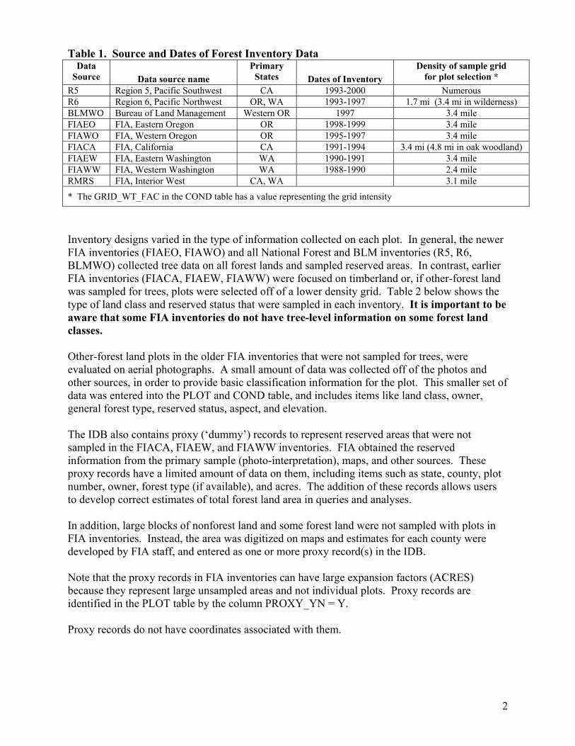
Table 1. Source and Dates of Forest Inventory Data

Data Source Data source name

Primary States Dates of Inventory

Density of sample grid for plot selection *

R5 Region 5, Pacific Southwest CA 1993-2000 Numerous R6 Region 6, Pacific Northwest OR, WA 1993-1997 1.7 mi (3.4 mi in wilderness) BLMWO Bureau of Land Management Western OR 1997 3.4 mile FIAEO FIA, Eastern Oregon OR 1998-1999 3.4 mile FIAWO FIA, Western Oregon OR 1995-1997 3.4 mile FIACA FIA, California CA 1991-1994 3.4 mi (4.8 mi in oak woodland) FIAEW FIA, Eastern Washington WA 1990-1991 3.4 mile FIAWW FIA, Western Washington WA 1988-1990 2.4 mile RMRS FIA, Interior West CA, WA 3.1 mile

* The GRID_WT_FAC in the COND table has a value representing the grid intensity

Inventory designs varied in the type of information collected on each plot. In general, the newer FIA inventories (FIAEO, FIAWO) and all National Forest and BLM inventories (R5, R6, BLMWO) collected tree data on all forest lands and sampled reserved areas. In contrast, earlier FIA inventories (FIACA, FIAEW, FIAWW) were focused on timberland or, if other-forest land was sampled for trees, plots were selected off of a lower density grid. Table 2 below shows the type of land class and reserved status that were sampled in each inventory. It is important to be aware that some FIA inventories do not have tree-level information on some forest land classes. Other-forest land plots in the older FIA inventories that were not sampled for trees, were evaluated on aerial photographs. A small amount of data was collected off of the photos and other sources, in order to provide basic classification information for the plot. This smaller set of data was entered into the PLOT and COND table, and includes items like land class, owner, general forest type, reserved status, aspect, and elevation. The IDB also contains proxy (‘dummy’) records to represent reserved areas that were not sampled in the FIACA, FIAEW, and FIAWW inventories. FIA obtained the reserved information from the primary sample (photo-interpretation), maps, and other sources. These proxy records have a limited amount of data on them, including items such as state, county, plot number, owner, forest type (if available), and acres. The addition of these records allows users to develop correct estimates of total forest land area in queries and analyses. In addition, large blocks of nonforest land and some forest land were not sampled with plots in FIA inventories. Instead, the area was digitized on maps and estimates for each county were developed by FIA staff, and entered as one or more proxy record(s) in the IDB. Note that the proxy records in FIA inventories can have large expansion factors (ACRES) because they represent large unsampled areas and not individual plots. Proxy records are identified in the PLOT table by the column PROXY_YN = Y. Proxy records do not have coordinates associated with them.

3

Area and Volume Expansion When summarizing the amount of land area within a category of interest, the ACRES column should be used (the exception to this is discussed below for FIACA woodland plots). When summarizing volume (or other tree-level, per-acre attribute), the ACRES_VOL column should be used to expand the per-acre value. For example, Net cubic volume = VOL_AC_NET_FT3 * ACRES_VOL. ACRES column Each condition class on a plot represents a certain amount of acres in the broad inventory area. ACRES is used to summarize the amount of land area within a given category (i.e. owner, forest type, state, national forest). ACRES is an estimate of land area based on various stratification schemes and methods that were appropriate for each inventory. Each DATA_SOURCE (R5, R6, BLMWO, and FIA) used slightly different techniques to develop an estimate for this column. FIA ACRES were calculated by FIA staff at the time of the original compilation. The IDB staff used stratification information provided by R5, R6, and BLMWO staff to calculate plot and condition class acres for NFS and BLM inventories. For R6, land area estimates published on the national website that tracks national forest land area (both proclaimed and administered) for each county in the country were used to stratify the plots. This method allows the total land area to match Bureau of Census figures for a given county. The stratification uses the amount of Proclaimed acres of total National Forest land within each county, summarized by wilderness and non-wilderness areas. The total number of NF plots within wilderness or non-wilderness locations in each county were divided into the total NF land area within the county (irregardless of specific National Forest) to derive the acres per plot. Users can then summarize the amount of acres using the Administered National Forest code (FOREST_OR_BLM_DISTRICT column), which is the most common way to analyze and report NFS data. Please see the technical document “Area_Expansion_R6_BLMWO.doc” for

Table 2. Information about the type of land that was sampled in each inventory.

Data Source Land classes sampled for trees

Ground Land Class codes

Reserved lands

sampled? Comment

R5 All forest land 20, 40’s Yes R6 All forest land 20, 40’s Yes BLMWO All forest land 20, 40’s Yes FIAEO All forest land 20, 40’s Yes Not all Juniper forest land was sampled FIAWO All forest land 20, 40’s Yes

FIACA Timberland and partial sample of woodland (other forest,44) 20, 44, 49 No Not all Woodland forest land was sampled

FIAEW Forest land 20, 40’s No

FIAWW Timberland only 20, 49 No ‘Other-forest’ or ‘Unproductive forest’ were not sampled

RMRS All forest land 20’s, 40’s Yes New to Version 2.0 Data from the Toiyabe National Forest in California and the Kaniksu National Forest in Washington were added to the IDB. For FIAEO, data from the Juniper inventory were added, where juniper forest land plots (GLC=43) on the east side of the Cascades were measured.

4

more information. The goal has always been to match the total acres per county in the IDB with the county land area published in the 1990 Bureau of Census reports (because inventory data were collected in the 90’s). For BLMWO, a count was made of the total number of plots in each county in the BLM database. Total land area by county was summarized from the 1995-1998 FIA inventory of western Oregon, for land owned by the BLM. The plot count was divided into the county area to derive the acres per plot, which was multiplied by the COND_WT to estimate ACRES. Please see the document “Area_Expansion_R6_BLMWO.doc” for more information. For R5, condition class acres were estimated from strata on map-based GIS layers. A count of subplots was divided into the area of mapped vegetative strata to estimate acres per subplot, which was multiplied by the number of subplots per condition to calculate ACRES. For FIA, stratification schemes varied by half-state and in general, included owner, land class, county, and survey unit as stratum identifiers. Plot counts within strata were divided into the stratum area to create an estimate of acres per plot, which was multiplied by the COND_WT to estimate ACRES. The sum of the ACRES across all conditions on one plot equals the acres represented by the individual plot location. Each row in the COND table has an estimate of land area (ACRES) associated with that condition on the plot. ACRES_VOL column ACRES_VOL is an area expansion factor used specifically to expand each per-acre column such as volume/acre or biomass/acre, to develop an estimate of population totals for an attribute of interest. Volume/acre estimates are available for a wide variety of live and dead tree attributes such as whole tree volume, merchantable volume, current annual growth volume, mortality volume, gross volume, net volume, etc. Biomass/acre estimates include above ground woody biomass, branch biomass, bark biomass, and bole biomass. Per-acre estimates are also available for down wood data, which should be summarized to the condition level before expansion. To expand any per-acre column, multiply the column by the ACRES_VOL column as follows: Attribute of interest = attribute/acre * ACRES_VOL For example, Volume= volume/ac * ACRES_VOL or Biomass=biomass/ac * ACRES_VOL The result provides an estimate of what the tree or piece of down wood represents across the inventory area (population totals). In many cases, ACRES equals ACRES_VOL. When these columns are different, it indicates that a different stratification scheme or sampling design was used to provide a more accurate estimate of tree volume or biomass. When ACRES_VOL contains a value, it indicates that the condition and plot were intentionally sampled for trees or down wood. It is important to use ACRES_VOL every time a per-acre attribute is expanded.

5

Expansion of Tree Mortality data Dead trees that are recent mortality are stored in the TREE_MORT table. A mortality tree is a dead tree that has died within the past 5 or 10 years of the current inventory date. The TREE_MORT table includes information about trees that died within the last 5 years (for R5, R6 and BLMWO) and trees that died during the FIA remeasurement period (about 10 years for FIACA, FIAEO, FIAWO, FIAWW, FIAEW). Note that for FIA, a mortality tree may or may not be standing. For NFS and BLM inventories, there was no previous measurement, so a recent mortality tree was estimated by field crews to have died sometime within the 5 years prior to the current inventory. All mortality trees for NFS and BLM are standing dead. Some important points need to be made about the use of mortality data on FIA plots. Mortality was tallied on remeasured (or reconstructed) subplots and conditions only. Because the design has changed over time, new subplots were installed in a different configuration. The inventories in the IDB contain the most recent measurement of inventory plots, including the subplots newly installed. Mortality was not measured on these new subplots in FIA inventories. In addition, mortality was only measured on condition class 1 – which was the condition installed and measured at the previous inventory. In the western Washington FIA inventory, half of the plots were not sampled for mortality. This requires a different area expansion factor to be used when expanding the per-acre tree estimates to population totals. The correct area expansion factor to use for mortality data in the TREE_MORT table is found in the COND table and called ACRES_VOL_MORT. For example: Mortality volume in cubic feet = VOL_AC_GRS_FT3 * ACRES_VOL_MORT Because mortality trees were not measured on every subplot and every condition, it may be more appropriate to use a weighted mean of the per-acre estimates, rather than expanding them to a population estimate. California’s woodland inventory conducted by FIA The FIACA inventory sampled all types of land classes on a 3.4-mile grid. Trees were measured on every timberland plot (GLC=20,49) and on a partial sample of all woodland (GLC=44) plots. Because of the partial sample, a different stratification scheme was used on the woodland plots, resulting in a second area expansion factor which must be used to expand all per-acre tree-level estimates (i.e. volume/acre) and to summarize most area information. IDB users need to be aware that the expansion factor called ACRES_VOL must be used when some area summaries are run for woodland land classes. Specifically, if columns that are based on tree data (forest type or stand size) are used to group data, the ACRES_VOL must be used. If a broader summary of forest land by land class is done (where forest type, etc are not used), the ACRES column can be used. Summaries at the county level If a summary is needed at the county level, link the COND_EXTRA table to the COND table by the COND_ID column, and use the expansion factors called ACRES_CNTY or ACRES_CNTY_VOL. Most FIA and all NFS inventories were designed at the Survey Unit level (group of contiguous counties) or National Forest level. The expansion factors ACRES or ACRES_VOL were developed from a stratification at these levels, and provide the most accurate estimates of area, volume, biomass, numbers of trees, etc for the population. For FIA inventories, a second stratification was conducted that incorporated county into the process. This

6

stratification resulted in the second set of expansion factors (ACRES_CNTY or ACRES_CNTY_VOL), which provide better population estimates for a given county. However, standard errors are known to be higher at the county level because the sample size per county (number of plots) is often insufficient to produce reliable results. In summary, the primary use of the inventory data in the IDB should be to provide information at the survey unit, state, National Forest, or BLM district level – which was how the inventories were originally designed. Users should be aware that summaries at the county level are possible (using the COND_EXTRA table) but the estimates are likely to be less reliable with larger standard errors. Note that FIA Oregon inventories and the BLM inventory included county as a component of the main stratification, therefore the ACRES and ACRES_VOL can be used reliably to develop county level estimates. A second county level stratification was not done on NFS lands, therefore the ACRES_CNTY or ACRES_CNTY_VOL are the same as ACRES or ACRES_VOL. For ease of use, the COND_EXTRA table contains entries for every record in the COND table, however only FIA and BLM inventories were actually stratified by county to create these expansion factors . Calculating a weighted average When calculating an average per-unit area estimate with inventory data, it should be weighted by the sampling grid density and the size of the condition class area where the tree or down wood was sampled. The weighting factor called SAMPLING_WT_FAC on the COND table should be used as the weight for all data except tree mortality data. When working with data in the TREE_MORT table, the weight called SAMPLING_WT_MORT_FAC should be used. Weighted means are normally calculated as follows: Weighted mean = (sum of SAMPLING_WT_FAC * Per-Acre Value) / (sum of SAMPLING_WT_FAC ) where SAMPLING_WT_FAC = (GRID_WT_FAC * COND_WT)

7

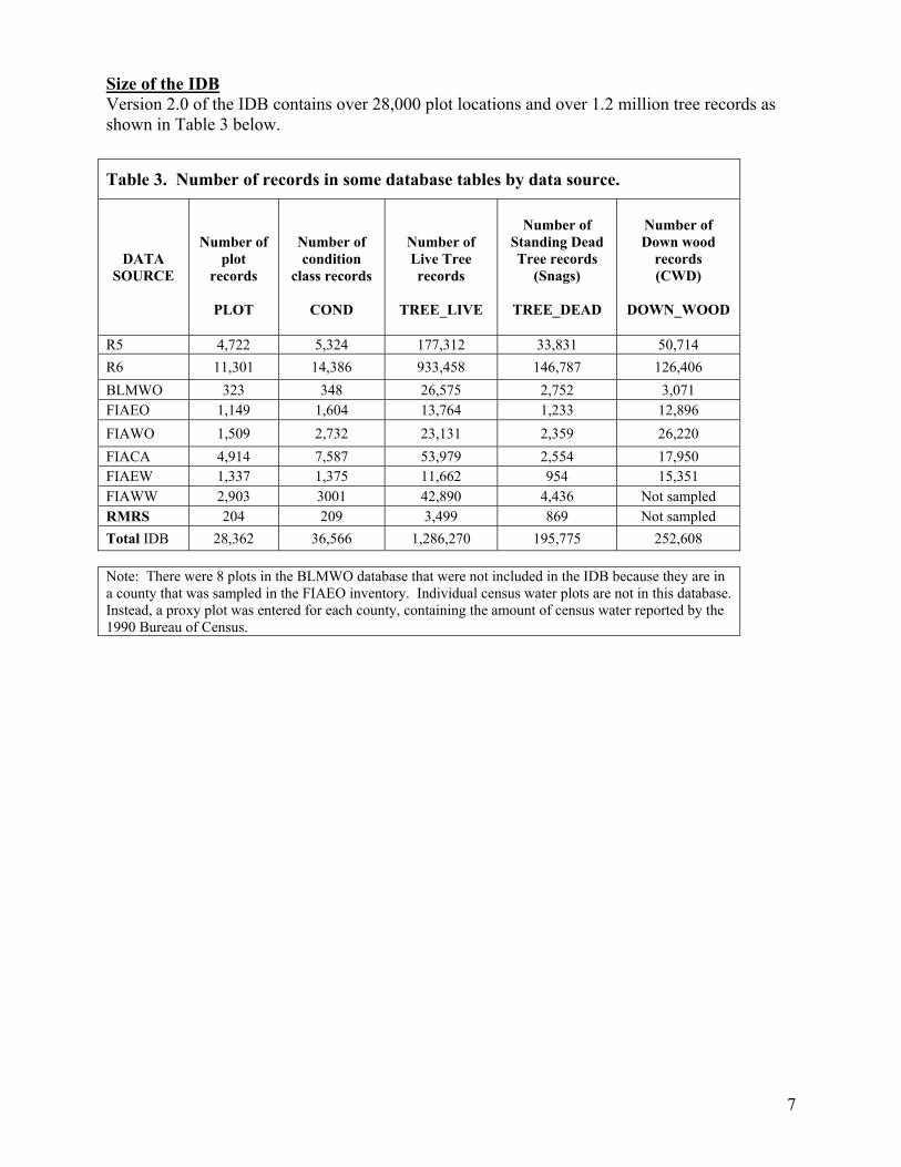
Size of the IDB Version 2.0 of the IDB contains over 28,000 plot locations and over 1.2 million tree records as shown in Table 3 below.

Table 3. Number of records in some database tables by data source.

DATA SOURCE

Number of plot

records

PLOT

Number of condition

class records

COND

Number of Live Tree records

TREE_LIVE

Number of

Standing Dead Tree records

(Snags)

TREE_DEAD

Number of Down wood

records (CWD)

DOWN_WOOD

R5 4,722 5,324 177,312 33,831 50,714 R6 11,301 14,386 933,458 146,787 126,406 BLMWO 323 348 26,575 2,752 3,071 FIAEO 1,149 1,604 13,764 1,233 12,896 FIAWO 1,509 2,732 23,131 2,359 26,220 FIACA 4,914 7,587 53,979 2,554 17,950 FIAEW 1,337 1,375 11,662 954 15,351 FIAWW 2,903 3001 42,890 4,436 Not sampled RMRS 204 209 3,499 869 Not sampled Total IDB 28,362 36,566 1,286,270 195,775 252,608

Note: There were 8 plots in the BLMWO database that were not included in the IDB because they are in a county that was sampled in the FIAEO inventory. Individual census water plots are not in this database. Instead, a proxy plot was entered for each county, containing the amount of census water reported by the 1990 Bureau of Census.

8

TABLES IN THE IDB:

9

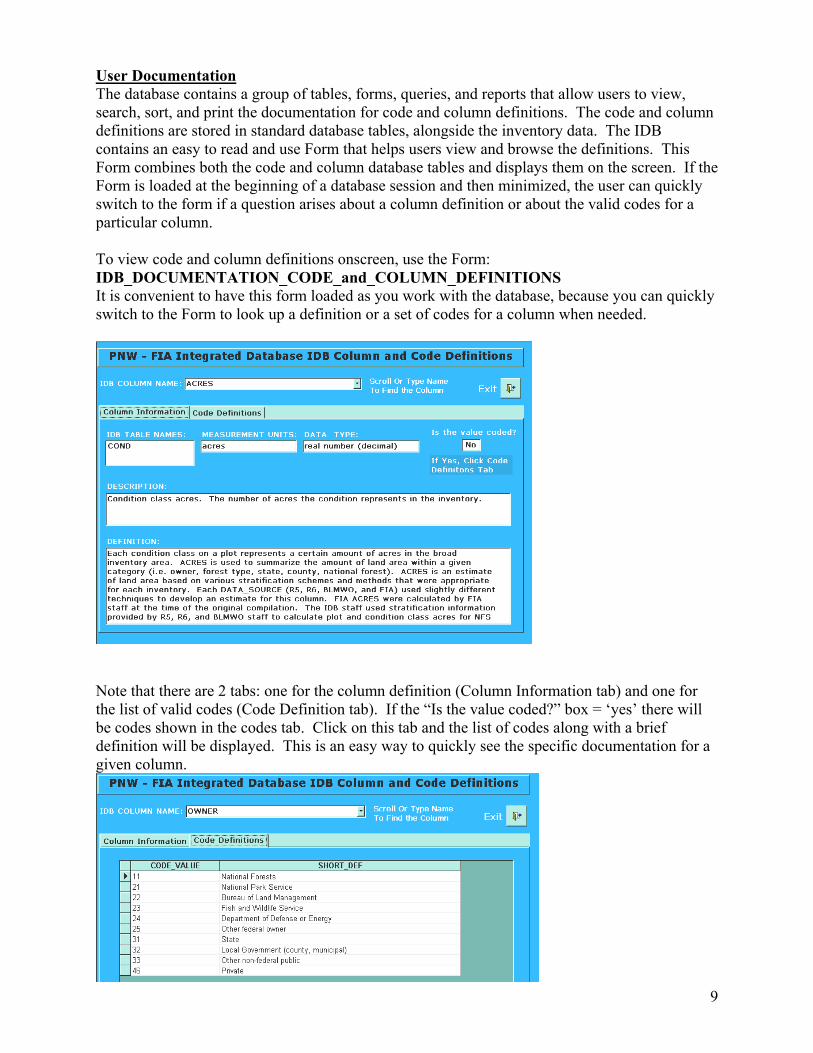
User Documentation The database contains a group of tables, forms, queries, and reports that allow users to view, search, sort, and print the documentation for code and column definitions. The code and column definitions are stored in standard database tables, alongside the inventory data. The IDB contains an easy to read and use Form that helps users view and browse the definitions. This Form combines both the code and column database tables and displays them on the screen. If the Form is loaded at the beginning of a database session and then minimized, the user can quickly switch to the form if a question arises about a column definition or about the valid codes for a particular column. To view code and column definitions onscreen, use the Form: IDB_DOCUMENTATION_CODE_and_COLUMN_DEFINITIONS It is convenient to have this form loaded as you work with the database, because you can quickly switch to the Form to look up a definition or a set of codes for a column when needed.

Note that there are 2 tabs: one for the column definition (Column Information tab) and one for the list of valid codes (Code Definition tab). If the “Is the value coded?” box = ‘yes’ there will be codes shown in the codes tab. Click on this tab and the list of codes along with a brief definition will be displayed. This is an easy way to quickly see the specific documentation for a given column.

10

To print column definitions use the Report Writer: IDB COLUMN DEFINITION REPORT To print code definitions use the Report Writer: IDB CODE DEFINITION REPORT

The output from the reports above have been stored as Adobe PDF files in the User Documentation directory on the CD. In addition, there is a PDF file that contains information about the structure of each database table, including the column name, measurement units, coded information, and the data type. The following documentation files can be printed to serve as a reference while using the IDB: 1_IDB_Vers2 _User Guide Color Coverpage.doc 2_IDB_Vers2_User Guide.doc 3_IDB_Vers2_TABLE_STRUCTURE.pdf 4_IDB_Vers2_COLUMN_LIST.pdf 5_IDB_Vers2_CODE_LIST.pdf 6_IDB_Vers2_COLUMN DEFINITIONS.pdf Technical Documentation The directory called “technical documentation“ contains a variety of documents that describe procedures used to calculate some of the data in the database. The goal of the IDB was to compile the calculated fields in the same way across inventories, whenever possible, using FIA procedures and methods. Because of inherent differences in inventory designs and collection techniques, this goal was not always attainable. In some cases, IDB staff went to other sources (i.e. FVS programs) to locate an appropriate equation or method for the National Forest and BLM data. These methods are described and documented. The technical documentation also includes all volume, stocking, biomass, and site index equations used in this database. IDB staff will continue to update, enhance, and add new technical documents over time.

11

IDB TABLE STRUCTURE AND RELATIONSHIPS Database Tables The current set of inventory tables includes: PLOT -General information about the sample plot COND -Condition class data, multiple conditions (rows) possible on a plot TREE_LIVE -Live tree data, including seedlings TREE_DEAD -Standing dead trees, died from all causes TREE_MORT -Recent mortality – trees that died from natural causes within 5-10 years (may be standing, down, or gone) TREE_SITE -Live tree data, high quality trees measured as site trees DOWN_WOOD -Down wood data >= 3” in diameter SUBPLOT -Subplot data, one row per condition per subplot on the plot STRATUM -Stratification information PLOT_COORDINATES -Contains fuzzed coordinates for each plot location PLOT_EXTRA -Additional information for each plot COND_EXTRA -Additional information for each condition There are also many metadata tables in the database that contain crosswalks of codes to a text name or description. For example, there is a table that contains the numeric species code, common name, and scientific name. These tables are useful to include in a query or report, so the actual text name is displayed instead of a numeric code. The following metadata tables are available in Version 2.0 of the IDB. More tables will be added to this group as relevant information or data become available. These tables can be linked to the inventory data tables via the appropriate numeric code to provide text names for things like tree species, counties, survey unit, state, National Forests, NFS and BLM districts, variants, owner and more. Metadata tables in the IDB: IDB_COUNTY_NAMES IDB_DIAMETER_CLASS_CONVERSIONS IDB_EQUATION_NUMBERS IDB_FOREST_TYPES IDB_FOREST_NAMES IDB_FTYPE_TO_RPA_FTYPE IDB_GLC_GROUP_DESCRIPTIONS IDB_OWNER_GROUPS IDB_PLANT_ASSOCIATIONS IDB_R6_DISTRICTS_ON_FORESTS IDB_TREE_SPECIES IDB_VARIANT_CODE_DESCRIPTIONS

12

Queries The IDB contains a variety of queries to summarize area and volume data within a number of different categories. Open the queries in design mode and enter selection criteria for areas of interest such as state, halfstate, national forest, data source, etc. See the code definitions for the appropriate codes to use. Queries also format and display code and column documentation. Some of the queries are shown below:

13

KEY fields The database has all necessary relationships established and pre-joined among all the inventory tables in the database. The naming convention for KEY fields in this is database is as follows: Each table has an ID field, which is a unique number for every row in the entire table. The name of the column always includes the table name before the word ID. The following list shows the primary key field in each table:

The COND_ID is the most commonly used KEY field in the database. This field is a unique number for every condition record in the COND table, and is required for most joins that users will make. It is present in every table except the plot level tables (see figure 1 below). The ALLTREE_ID is a sequential number that uniquely identifies each individual tree (live and dead) in the entire database. This ID was created because there was overlap and duplication of individual trees among some tree tables. A live tree can also be a site tree, and a mortality tree can also be a snag. The ALLTREE_ID uniquely identifies all individual trees across all DATA_SOURCES and tables. This number allows users to combine live and dead trees if desired, and still retain a unique ID for the new table. If one tree is also in another table, both records will have the same ALLTREE_ID. PLOT_ID is a sequential number that uniquely identifies each plot (row) in the entire PLOT table. It is recommended that PLOT_ID be used when summarizing or grouping data by plot, because the original plot numbers (PLOT) are not unique in the database. For example, in FIA data, a plot number is unique within state and county; for R5 it is unique within region and National Forest; and for R6 plot number is unique for the entire region. People familiar with FIA data should note that the combination of state, county and plot are not unique across all inventories in the IDB, and will not identify an individual plot location. Because of this variability in uniqueness from the many data sources in this database, it is recommended that the column PLOT_ID be used to uniquely identify every plot location in this database. This ID is unique across all data sources and all inventories.

Table Name Key field (unique row identifier)

PLOT PLOT_ID COND COND_ID TREE_LIVE TREE_LIVE_ID TREE_DEAD TREE_DEAD_ID TREE_MORT TREE_MORT _ID TREE_SITE TREE_SITE_ID DOWN_WOOD DOWN_WOOD_ID SUBPLOT SUBPLOT_ID STRATUM STRATUM_ID PLOT_COORDINATES PLOT_ID PLOT_EXTRA PLOT_ID COND_EXTRA COND_ID

14

In previous versions of the IDB, the PLOT table was the only place where the original plot number is stored. However, for convenience, the PLOT, CNTY, STATE, FOREST_OR_BLM_DISTRICT, and COND_CLASS codes were added to the COND, TREE_LIVE, TREE_DEAD, and DOWN_WOOD table. Remember that the PLOT_ ID and COND_ID are the best fields to link tables together. For users who wish to link tables by columns other than the PLOT_ ID and COND_ID, use the following combination of columns for different data sources: All FIA: link on STATE, CTY, PLOT, COND_CLASS R6 and BLMWO: link on PLOT and COND_CLASS R5: link on FOREST_OR_BLM_DISTRICT, PLOT, and COND_CLASS All the relationships are predefined to insure that tables are automatically linked by the appropriate KEY field when the user creates new queries. If a new table is created by the user, the relationships must be re-established manually by dragging a line from one ID to another ID in a second table. Figure 1 below illustrates the IDB table relationships with KEY fields. All relationships have been pre-linked within Access, reducing potential errors when developing queries or reports. However, if new tables are created during an analysis of the data, the links will be lost. The most common link is between COND and each of the 5 tree or down wood tables.

TREE_LIVE_ID COND_ID SUBPLOT_ID ALLTREE_ID

TREE_LIVE TABLE

STRATUM TABLE

DOWN_WOOD_IDCOND_ID SUBPLOT_ID TRANSECT_ID

DOWN_WOODTABLE

TREE_DEAD_ID COND_ID SUBPLOT_ID ALLTREE_ID

TREE_DEAD TABLE

PLOT_ID STRATUM_ID STRATUM_VOL__ID

COND_ID PLOT_ID

COND TABLE

PLOT TABLE

SUBPLOT_ID COND_ID

TREE_MORT_ID COND_ID SUBPLOT_ID ALLTREE_ID

TREE_MORT TABLE

TREE_SITE_ID COND_ID SUBPLOT_ID ALLTREE_ID

TREE_SITE TABLE

STRATUM_ ID

SUBPLOT TABLE

15

Seedlings Seedlings are live trees < 1 inch in diameter, and identified by the column SEEDLING_YN=Y. For R5, R6, and BLMWO, seedlings were group counted during data collection and entered into the live tree database as one line of data. Trees/acre was calculated for each seedling group by first calculating the value for 1 seedling and then multiplying this value by the seedling count. This expanded value is stored in the database, therefore some seedling data may appear to be unusually large in comparison with other tree data. Each seedling has a stocking value calculated for it, which has been converted to a stocking estimate for the seedling group. Confidentiality FIA is mandated by Law (Privacy Amendment: H.R.3423 Department of the Interior and Related Agencies Appropriations Act, 2000 (November 17, 1999)) not to disclose any information that can be tied back to an individual landowner. For this reason we can not give the actual true plot locations out to anyone, because they might be able to use GIS or tax records to ascertain the individual owner of the plot. We use a randomized offset for each plot to mask the true location. This is called fuzzing. For all plots in the IDB that are on lands in public ownership (such as State, Federal and municipal), we randomly offset the coordinates up to 1/2 mile in any direction. We further randomly selected 5% of these plots and offset them by up to 1 mile (instead of the 1/2 mile). Plots in the IDB that are on privately owned lands were fuzzed to 100 seconds of latitude and longitude, which is up to about 2 miles. Using this method, plots were not allowed to jump county lines when we fuzzed the coordinates. Simply fuzzing the plot coordinates does not truly protect us from disclosing data that could be tied to an individual owner, and thus does not comply with the law. For instance, a plot offset by a half mile (or even two miles) in the center of the Warm Springs Reservation would still be in the Reservation, so all data associated with that plot could be tied to an individual owner, in this case the Consolidated Tribes of the Warm Springs. So, the data for a percentage of the IDB plots on privately owned lands have been swapped with the data from a similar plot in the county. In this way, there is always a chance that the data can not be tied back to the single owner, even with a GIS system, thus FIA would still be complying with the law. The swapping method was designed to minimize the affects on analysis. And since no plots are allowed to move to another county, analysis at the county level will not be affected. However, a group of plots from a part of a county might show effects of fuzzing and swapping, with the fewer the number of plots chosen, the greater the possible effect. The ‘fuzzed’ coordinates have been included in the IDB and are stored in the PLOT_COORDINATES table. There is one set of latitude and longitude coordinates for each plot record, except for the PROXY plots. Since PROXY plots are essentially placeholders for estimated unsampled area in the inventory, they are not actual plots. If exact plot coordinates are needed, please contact the FIA program in Portland, OR to determine if we can accommodate your request. Specific protocols for the use of FIA coordinates have been established, and permission is granted on a case by case basis. In addition to the fuzzing of coordinates, the ownership data for private owners in the IDB have been grouped into a general code of ‘private’. For more information on this issue, contact Dale Weyermann (503-808-2042) or the Program Manager, Susan Willits (503-808-2066).

16

Use of the STRATUM table The STRATUM table contains all the necessary data and information about each strata for each inventory (DATA_SOURCE). This table is required to correctly estimate variance or standard errors for an area or volume summary. This table is especially important when working with FIA data because it provides information on both the primary and secondary samples of the double-sample for stratification inventory design. If you are working with an area summary table, link the STRATUM_ID in the STRATUM table to the STRATUM_ID in the PLOT table. If you are working with a volume summary table, link the STRATUM_ID in the STRATUM table to the STRATUM_VOL_ID in the PLOT table. For an extensive discussion of statistical methods for estimating population totals, means, and associated standard errors for each inventory in the IDB, please read the IDB document called Alternative_Estimation_procedures.doc. This document contains a publication (in press) by Tara Barrett entitled Estimation procedures for the combined 1990s periodic inventories of California, Oregon, and Washington. For more information on the use of the STRATUM table, please contact Tara Barrett, Research Biometrician (503-808-2041).

17

Contents of the Integrated Database CD FOLDER: IDB Database Version 2.0 IDB_Version_2.zip UP6_Update Notice for Version 2.0.doc Intro Letter.doc CD Cover 2005.mfp (Media Face CD label) FOLDER: User Documentation V 2.0 1_IDB_Vers2 _User Guide Color Coverpage.doc 2_IDB_Vers2_User Guide.doc 3_IDB_Vers2_TABLE_STRUCTURE.pdf 4_IDB_Vers2_COLUMN_LIST.pdf 5_IDB_Vers2_CODE_LIST.pdf 6_IDB_Vers2_COLUMN DEFINITIONS.pdf Combined Documentation files.pdf IDB_Vers2_TABLE_STRUCTURE.xls

FOLDER: Field Manuals

Technical Documentation V 2.0 Area Expansion_R5.doc Area_Expansion_R6_BLMWO.doc Biomass equations.doc BLM Plant Association crosswalk to Halls codes.xls Census Water.doc Condition Class.doc County Code Corrections_R6_BLM.doc Cull species_information.doc Dead Tree Documentation.doc Down Wood Inventories in the IDB.doc Down Wood Calculation_Methods_Ecological Indicators paper.pdf

18

Down Wood Paper on the Line Intersect method.pdf Down Wood Decay Class codes.doc Diameter increments.DOC Dunnings SITE CLASS table.xls Estimation of Mortality Rates.doc Estimation Procedures GTR 597.pdf Forest type algorithm.doc FVS Crosswalk from Plant Association to SI.xls Ground land class.doc Height estimation in IDB_R5_R6_BLM.doc Height estimation_FVS equations.doc MAI_site classes.doc Mortality Rates for R5, R6 BLM.xls Mortality_USING THE TREE_MORT TABLE.doc Omerniks Ecoregions.doc Plant Association Codes.doc Site Index and MAI_Publication.pdf Site Index.doc Stand Age.doc Stand position.doc Stand size.doc Stocking and stocking equations.doc Table of differences between snags and mortality sampling.doc TPA TPH calculation.doc TREE SPECIES AND SPECIFIC GRAVITY.doc Volume equations.doc