Embed Size (px)
Citation preview
TECHNICAL REPORT STANDARD TITLE PAGE
1. Report No. 2. Governm<1nt AccH•ion No. 3. Recipient'• Cat.IQll No.
FHWA/TX-91/1123-4 4. Title end Subtitle 5. Report Date
MODULUS 4.0, User's Manual January 1991 e. PerforminQ Organization Code
7. Author(sl 8. ,,_rforrnin; Otg41nizetion Rtiport: No.
Tom Scullion, Chester Michalak Research Report 1123-4 9. Performing Organization Name end Address 10. Work Unit No.
Texas Transportation Institute Texas A&M University 11. Contrect or Gr•nt No.
College Station, Texas 77843-3135 Study No. 2-18-87-1123 12. SponeorinQ Agency Name end Add., .. 13. Type of Report end Period Cow"'d
Texas State Department of Highways and Public Final September 1988 Transportation, Transportation Planning Division September 1990
P.O. Box 5051, Austin, Texas 78763 14. Sponsoring Agency Code
15. Suppfe'mentary Notes
Research performed in cooperation with DOT, FHWA Research Study Title "Nondestructive Test Procedures for Analyzing the Structural Condition of Pavements" 16. Abstract
The MODULUS program, a modulus backcalculation system described in this report, has been developed by the Texas Transportation Institute for the Texas Department of Highways and Public Transportation. See TTI Research Reports 1123-1 and 1123-2 for background and technical details. This system is intended to be used when analyzing data collected with only the Falling Weight Deflectometer. The following enhancements have been made in this version of the software:
1) Automatic calculation of a depth to a stiff layer (H4}, which can be overwritten by the user.
2) Automatic calculation of weighting factors for each sensor. 3) Detection of non-linearity in the subgrade, and automatic selection of the
optimum numbers of sensors to use in the backcalculation process. 4) The use of the corps of Engineers WESS linear elastic program which is
considerably faster than existing programs and has no copyright restrictions. 5) Inclusion of a routine to permit manual input of deflection bowl data. One minor restriction on this version of MODULUS is the four of the deflection
sensors must be located at offsets of 0, 12, 24, 36 inches from the center of the load plate. It does not matter which four; for example, other sensors could be included at eight and 18 inches.
The MODULUS system has the three following subsystems: Subsystem 1 Data Input, Subsystem 2 MODULUS Backcalculation, and Subsystem 3 Plot Deflection. 17. Key Wordo 18. Distribution St•tem•nt
Modulus, Backcalculation, Falling Weight No Restrictions Deflectometer, Non-linearity, Linear- Available through the National Technical elasticity Information Service
5285 Port Royal Sorinqfield, Virginia 22161
I 19. Security Clenif. !of th0o "'port! 20. Security Clnoif. (of !hie P'IQ•l 21. No.of Pao•• 22. Price
Unclassified Unclassified 46
Form DOT F 1700. 7 (8-69)

MODULUS 4.0: USER'S MANUAL
by
Tom Scullion Chester Michalak
Research Report 1123-4 Research Study Number 2-18-87-1123
Study Title: "Nondestructive Test Procedures for Analyzing Structural Condition of Pavements"
Conducted for
Texas State Department of Highways and Public Transportation
by
Texas Transportation Institute
January 1991

MODULUS 4.0 USER'S MANUAL ABSTRACT
The MODULUS program, a modulus backcalculation system described in this report, has been developed by the Texas Transportation Institute for the Texas State Department of Highways and Public Transportation. See TTI Research Reports 1123-1 and 1123-3 for background and technical details. This system is intended to be used when analyzing data collected with only the Falling Weight Deflectometer. The following enhancements have been made in this version of the software:
1) Automatic calculation of a depth to a stiff layer (H4), which can be overwritten by the user.
2) Automatic calculation of weighing factors for each sensor. 3) Detection of non-linearity in the subgrade, and automatic
selection of the optimum numbers of sensors to use in the backcalculation process.
4) The use of the corps of Engineers WESS linear elastic program which is considerably faster than existing programs and has no copyright restrictions.
5} Inclusion of a routine to permit manual input of deflection bowl data.
One minor restriction on this version of MODULUS is that four of the deflection sensors must be located at offsets of 0, 12, 24, and 36 inches from the center of the load plate. It does not matter which four; for example, other sensors could be included at 8 and 18 inches.
The MODULUS system has the three following subsystems.
Subsystem 1 Data Input This subsystem has two options: either the user can manually input
deflection bowl data, or it can be automatically read from the field diskette (currently Dynatest versions 9, 10 and 20 data formats only).
This subsystem creates an input file for the modulus backcalculation procedure. The field diskette file must have a .FWD extension, and the created file is given the extension .OUT. This subsystem may be skipped if the .OUT file already exists.
;

Subsystem 2 Modulus Backcalculation This subsystem reads the .OUT file, performs the backcalculation and
creates a .DAT file which contains the calculated E values. Three options are available depending on the level of familiarity the user has with backcalculation schemes.
Subsystem 3 Plot Deflection This subsystem graphically displays the data stored in the .DAT file
and performs subsectioning. Any technical questions regarding this software should be directed to
Tom Scullion at the following address:
Pavement Systems Program Texas Transportation Institute Texas A&M University College Station Texas 77843 (409} 845-9913
ii

METRIC (SI*) CONVERSION FACTORS
APPROXIMATE CONVERSIONS TO SI UNITS APPROXIMATE CONVERSIONS TO SI UNITS
S,mbol Wheft You Know Multlply By To Find S,mbol Symbol Wh•n You Know Multlply By To Find Symbol
LENGTH LENGTH .. - millimetres 0.039 Inches In mm
In Inches 2.54 centimetres cm - m metres 3.28 feet ft ft feet 0.3048 metres m -yd yards 0.914 - m metres 1.09 yards yd
metres m .. km kilometres 0.621 miles mi ml miles 1.61 kilometres km --
- AREA -AREA -
- mm2 millimetres squared 0.0016 square Inches ln1
ln1 square Inches 645.2 centimetres squared cm 1 -- m' metres squared 10.764 square feet ft2 -ft' square feet 0.0929 metres squared m• km• kilometres squared 0.39 square miles ml1 -yd• square yards 0.836 metres squared m• .. - ha hectores (10 000 m') 2.53 acres ac
m11 square miles 2.59 kllometres squared km1 -...... ac acres 0.395 hectares ha MASS (weight) ...... -- -.. - g grams 0.0353 ounces oz
MASS (weight) - kg kilograms 2.205 pounds lb --- Mg megagrams (1 000 kg) 1.103 short tons T oz ounces 28.35 grams g -lb pounds 0.454 kilograms kg ... -- VOLUME T short tons (2000 lb) 0.907 megagrams Mg -
ml millilitres 0.034 fluid ounces fl oz - l litres 0.264 gallons gal VOLUME -
m• metres cubed 35.315 cubic feet ft> --- m• metres cubed 1.308 cubic yards yd• fl oz fluld ounces 29.57 mlllllltres ml -gal gallons 3.785 litres L -ftS cubic feet 0.0328 metres cubed mi .. - TEMPERATURE (exact) -yd• cubic yards 0.0765 metres cubed m• -- oC Celsius 9/5 (then Fahrenheit OF
NOTE: Volumes greater than 1000 L shall be shown In m•. - - temperature add 32) temperature
- Of - Of' 32 98.8 212 -TEMPERATURE (exact) ;; - -f I I • ~ I I ~~I • I ~I ~ I
1~ I I I
1~ I I . 2?0J !t I 1()() f t i i I t , r i
-40 -20 0 20 40 60 80 • -.. "C 37 °C Of Fahrenheit 519 (after Celslus oC temperature subtracting 32) temperature These factors conform to the requlr•ment of FHWA Order 5190.1A.
• SI Is the symbol for the International System of Measurements

DISCLAIMER
The contents of this report reflect the view of the authors who are respons·ible for the opinions, findings, and conclusions presented herein. The contents do not necessarily reflect the official view or policies of the Federal Highway Administration. This report does not constitute a standard, specifications, or regulations.
There is no invention or discovery conceived or reduced to practice in the course of or under this contract; including any art, method, process, machine, manufacture, design or composition of matter; or any new and useful improvement thereof; or any variety of plant which is or may be patentable under the patent law of the United States of America or any foreign country.
iv

IMPLEMENTATION STATEMENT
The Texas SDHPT is currently implementing a new Flexible Pavement Design System developed under study 455. A crucial input to that system is the subgrade resilient moduli value and its variance along the highway. Both of these can be readily calculated from Falling Weight Deflectometer data using the system described in this report.
The version of MODULUS described in this report uses WESLEA as the linear elastic calculation program. The system does not contain any proprietary software.
v

PREFACE
Other Reports in the 1123 series include: Report 1123-1 "A Microcomputer Based Procedure to Backcalculation Layer Moduli from FWD Data" which describes the calculation procedures in MODULUS 2.0, and the segmentation procedures. Report 1123-2 "Field Evaluation of the Multidepth Deflectometer" describes the MDD, the installation procedure and typical results obtained. This device provides the best means of validating modulus backcalculation procedures. Report 1123-3 "Expansion and Validation of the Modulus Backcalculation System"
vi

ABSTRACT DISCLAIMER
TABLE OF CONTENTS
IMPLEMENTATION STATEMENT . . . . PREFACE • . . . . . . . . I. INTRODUCTION ....... .
1.1 Getting Started . . ..... . 1.2 System Requirements •.•...•.
Page i
. . . . . iv • it • • v
. vi . . . . I
. . . . . . . . I
1 1.3 File Naming Convention . . . . . . . . . . . . 1
II. RUNNING THE PROGRAM . . . . . . . . . . . . 4 2.1 Starting the Program . . . . . . . . . 4 2.2 Main Program Menu Options .
III. OPTION 1 INPUT DATA CONVERSION OPTION 3.1 Convert .FWD to .OUT Data ..... 3.2 Manual Input of Deflection Bowl Data
IV. OPTION 2 MODULUS BACKCALCULATION PROCEDURE . 4.1 Using the Modulus Backcalculation Menu Options 4.2 Option 1 - Fixed Designs ... .
• • • • 4
. . . • • 7
7
. 12
. 16
. 18
4.3 Option 2 - Input Material Types ....... . . • 19
. . 19
4.4 Option 3 - Run a Full Analysis ............ 23 V. OPTION 3 PLOT DEFLECTION AND/OR MODULI VALUES PROGRAM . 27
VI. PR I NT RESULTS PROGRAM . . . . . . . . . . . 31
VII. CUSTOMIZING FIXED DESIGNS . . . . . . . . . . . . . . . . 35
vii

LIST OF TABLES
I. Modulus Defaults for the Eight Fixed Designs (ksi)
viii
Page • 21

LIST OF FIGURES
1. Main Program Menu Screen 2. Data Input Screen .... 3. Data Conversion Screen .. 4. Deflection Bowl Manual Entry Form 5. Input/Output File Information 6. Modulus Backcalculation Menu . 7. Existing Fixed Designs .... . 8. Input Material Types ..... . 9. Input Base and Subgrade Types
10. Full Analysis ....... .
Page 5
. . 10
. 11
. . • • 14
. 17
17
. . • 20
. • • • • 24
• • • • • 24
• • 25
11. Setup for Graphics . . . . . . . . . . . . . . . 28 12. Plot for Subgrade Module Values for a Section of FM 2818 ... 30 13. Print Results Menu ...... . 14. Summary Listing ...... . 15. Detailed Bowl by Bowl Listing
ix
• • • 32
. . 33 • • 34

1.1 Getting Started
CHAPTER I INTRODUCTION
The TTI MODULUS Analysis System program is distributed on a 5 1/4" or 3 1/2" high density disk. To make backup copies of this diskette use the DISKCOPY command from DOS to insure that all the files are copied to the backup diskette. It is recommended that the user create a subdirectory called MODULUS and then copy the entire distribution diskette into that subdirectory.
1.2 System Requirements Minimum system requirements to run the program are:
• IBM AT or compatible microcomputer. • 640 Kb of RAM. • DOS (version 3.00 or later) operating system. • Math coprocessor chip (80287, 80387, or similar). • A hard disk with IMB of available storage space. • A EGA or VGA graphics card with 256 Kb of screen memory and a
compatible RGB or monochrome monitor. • Printer.
It is recommended that an advanced microcomputer, a 286 or even a 386 based machine, be used in order to minimize program execution time.
1.3 File Naming Conventions The TTI MODULUS Analysis Systems program uses several types of files.
The type of each of these files is identified by the three letter extension to the filename:
• .LBR: Input/output screen display library. • .WES: A file produced by the MODBAC program. It contains input
data for the WESS program. • .DAI: These files contain the final results .
. DA2: The PRMODRES program uses these files to produce summary and detailed output tables which can be sent to a printer.
1

•TMP.DEF: This file contains input information provided by the user when selecting the full analysis backcalculation option. The information is later used by the MODBAC, WESS, and SEARCH programs.
•WES.RES: This file stores the normalized deflection data basis that are calculated by the WESS program. The file is used by the same programs as TMP.DEF.
•TMPl.DEF: This files contain default information for 24 fixed to TMP24.DEF pavement designs. If any of the fixed TMPI.DEF -
TMP24.0EF designs are selected, the corresponding file is renamed to TMP.DEF and used as input to the search routine.
•WESI.RES: These files contain the default deflection data base, they are renamed to WES.RES and used as input to the search routine.
•.OAT: Files with this extension store deflection readings and corresponding backcalculated moduli for each test point. This data is used by the DELINIAT program.
The DESIGN.DAT file contains the default names for the fixed analysis option of the modulus backcalculation subsystem. See the section on "Customizing Fixed Designs" for instructions on how the user can create its own fixed designs. The DEFAULT.DAT file stores default values for options two and three of the modulus backcalculation subsystem.
•DEFAULT.DAT: This file stores values used in the previous run of modulus backcalculation program. The values are displayed as default inputs during current execution of the program.
•DESIGNS.DAT: This file contains the name descriptions for the 24 existing fixed designs.
•.EXE: Identifies executable files. •.FWD: The field input file as obtained from the Falling Weight
Deflectometer.
2

•.OUT:
•DEPTHS.OUT:
These files are produced by the FWDREAD program. They contain deflection information extracted from either the FWD files (.FWD) or manually input into the system. Contains the depth to bedrock as calculated by the MODBAC.FOR program. The values are printed in the summary report.
•ZABSOLUT.OUT: Stores the ABSOLUTE error values of the fit as calculated by the SEARCH.FOR program. These values are also printed in the summary report.
•STATS.OUT: Stores the mean and standard deviation for the depths to bedrock numbers. These values are presented in the summary report.
•.VAL: This is a special file containing Poisson Ratio values for each pavement layer. This particular file is only used for output purposes by the PRMODRES program.
•.BAT: Batch files used for installation of the system onto the hard disk and for setting up and starting the program.
3

2.1 Starting the Program
CHAPTER II RUNNING THE PROGRAM
To run the TTI MODULUS Analysis System programs, make the MODULUS subdirectory active by typing CD\MODULUS after the DOS prompt. If another drive is active, type the letter of the drive where the system has been installed and press <ENTER>; then type CD\MODULUS.
Once in the MODULUS directory, type MODULUS followed by <ENTER> to start the program. After a few seconds, the introductory screen will be displayed. At this time the main program should appear on the screen, see Figure 1. 2.2 Main Program Menu Options
The Main Program Menu screen allows the selection of any of the four available programs. To execute any of the programs, use the up/down arrow keys to highlight the selection and press <ENTER>. All menus in this package work in the same way.
The following programs are available: •Convert FWD data to INPUT data: This program builds the .OUT file which contains the FWD deflection bowls for later processing. Two options are available: 1. Manual input of load and deflection data. 2. Automatic read of Dynatest FWD field diskette.
•Run Modulus Backcalculation Program: This option allows the user to execute the Modulus Backcalculation (MODULUS) program. This program uses INPUT files (files with the .OUT extension) that have been converted from FWD files using option one above. It can also process files that have been custom-made using a text editor or similar program.
•Plot Deflection and/or Moduli values: Select this option to produce plots of deflection data or backcalculated moduli values, as a function of project length. The program uses a cumulative difference algorithm to achieve unit delineation for either deflection and moduli data. The delineation approach is useful for identifying
4

MODULUS MAIN MENU PROGRAM
*l) Input Data Conversion Options *2) Run Modulus Backcalculation program* *3) Plot Deflection and/or Moduli values*
*4) Print results of latest analysis* *5) Exit to DOS*
Use the t or l keys or enter the option NUMBER and press <ENTER>
V4.0
(C) Copyright 1989, Texas Transportation Institute. All Rights Reserved
Figure I. Main Program Menu Screen.
5

units of sections or stations that present similar structural behavior. This option will also plot the absolute error and depth to bedrock data.
•Print results of latest analysis: This option permits the user to skip directly to the Print Menu in order to obtain summary and/or detailed printouts of the last analysis performed by the Modulus Back Calculation program.
To finish a session just select option five to exit to DOS.
6

CHAPTER III OPTION 1 - INPUT DATA CONVERSION OPTION
The first screen within the input data conversion option is shown in Figure 2. To get data into the system the user has two options. The first is the automatic conversion of the Oynatest field diskette file into the input data format for MODULUS. The second is a screen to manually input deflection data. Both are describe below.
3.1 Convert .FWD to .OUT Data The format used in the Dynatest FWD files is highly elaborate, and
most of the information that they contain is not relevant to the programs contained in the TTI MODULUS Analysis System. Consequently, a program capable of extracting the specific data was developed. This program extracts the following variables from a FWD file: district number, county number, highway prefix and number, mile point position of the station (to 3 decimal places), and load and deflection readings (up to seven) for a pre-specified drop along the length of a project. The program then stores this information in a new file and appends to its name the extension .OUT. These files form the actual input to the Modulus Backcalculation program and are hereon referred to as INPUT or .OUT files. In general during FWD testing one or more drops are made at one location. This program can handle from one to eight drops per location. The user will be requested to select one of the eight drops for processing.
To start the FWD conversion program, select option one from the menu and press <ENTER>. A window will appear in the lower part of the screen asking you to verify your choice. Enter <Y> if the choice is correct.
After a few moments, the program input screen (Figure 3) is displayed. There are five fields of required information that the user needs to input before the program can run. These are:
•DRIVE WHERE THE FWD FILE RESIDES: Enter the letter identifier of the drive where the FWD file to be converted is stored. If the FWD file is in the hard disk, enter the letter of the drive from which the program is running. If the file resides in a floppy disk, enter the letter of that drive. Finish this input by pressing <ENTER>.
7

•FWD DATA FILENAME: In this field enter the name of the FWD file to be converted. Enter the name of the file, up to eight alphanumeric characters, without entering the extension name (it will be automatically appended to the name you entered) and press <ENTER>. In Texas this filename is a combination of county number and highway name. To see a listing of all FWD files residing in the selected drive press <Fl>. To select a file, use the up/down arrows until the desired file is highlighted then press <ENTER>.
eGUTPUT FILE NAME: Supply the name of the output file. It can also be up to eight characters long, and the .OUT extension will be automatically appended. Again press <ENTER> to finish this input.
•NUMBER OF DROPS RECORDED AT EACH POINT: In this field the number of drops (up to eight) performed at each point or station during the test will be automatically displayed.
•NUMBER OF FWD DROP TO USE AT EACH POINT: At this point, enter the number of the drop to be analyzed. Frequently four drops are recorded at different load levels, e.g., 5,000, 8,000, 12,000, and 15,000 pounds. This option permits the user to select the load level of interest.
Check the input carefully. If a mistake has been made, press the <ESC> key, and the cursor will be set back to the beginning of the input process at the position of the drive letter designator. Press <ENTER> to validate the entries until the incorrect one is reached. To change it just enter the new value or name and press <ENTER> to validate it. Keep on pressing <ENTER> until the last field is reached. If it is also correct, press <ENTER> once again to validate that entry.
Pressing this last <ENTER> will start the conversion process, which should take about five to 10 seconds depending on the disk access speed and the length of the file being converted.
8

When the program has successfully executed, a window with the following message will be displayed:
FILE XXXXXXXX.OUT CONTAINS ### POINTS. where XXXXXXXX corresponds to the .OUT file name and ### to the number of points or stations stored in the file.
As a last option, the program will prompt to determine if another file is to be processed. Enter <Y> to extract another FWD file. To quit, enter <N> and press <ENTER> in order to go back to the Main Program Menu.
9

MODULUS INPUT DATA OPTIONS MENU
*l) Convert .FWD to .OUT Data *2) Enter .OUT Data Manually *3) Return to MAIN MENU
V4.0
Use the t amd i keys or enter the option NUMBER and press <ENTER>
Figure 2. Data Input Screen.
10

MODULUS FALLING WEIGHT DEFLECTOMETER DATA CONVERSION
PROGRAM INPUT SCREEN
DRIVE WHERE FWD FILE RESIDES - - - - - - - - - - - X FWD DATA FILENAME - - - - - - - - - - XXXXXXXX.FWD OUTPUT FILE NAME - - - - - - - - - - - XXXXXXXX.OUT NUMBER OF DROPS RECORDED AT EACH POINT - - - - X NUMBER OF FWD DROP TO USE FOR CONVERSION - - - - - X PROCESS ANOTHER FILE? - - - - - - - - - - - - - - X
V4.0
(C) Copyright 1989, Texas Transportation Institute. All Rights Reserved
Figure 3. Data Conversion Screen.
11

3.2 Manual Input of Deflection Bowl Data To start the manual deflection bowl data input program, select option
two from the input data menu and press <ENTER>. A window will appear asking you to verify your choice. Enter <Y> if the choice is correct.
The manual deflection bowl data input screen (Figure 4) will be displayed. The user will be asked to supply the following information to create the file:
eQUTPUT FILE NAME: Enter the name of the file, up to right alphanumeric characters. Note that the extension .OUT will be appended automatically to the name entered by the user.
•NUMBER OF BOWLS TO BE ENTERED: In this field enter the total number of deflection bowls you intend to enter manually.
•DISTRICT: Enter the district number in this field. (2 digits)
•COUNTY: Enter the SDHPT county number in the field. (3 digits)
•HIGHWAY: In this field enter the SDHPT highway prefix and number. (six alphanumerics}
•ENTER INFORMATION FOR BOWL NO.: In this field the program will display the number of the deflection bowls for which the user is entering deflection data.
•STATION OR MILEPOST: In this field enter the milepost (to three decimal places) where the deflection bowl was measured.
•LANE: Enter the lane (R or L) in which the deflection bowl was measured.
•LOAD: In this field enter the load in pounds used for the deflection test drop.
•WI to W7: Enter the deflection in mils measured at each of the FWD sensors one through seven for this deflection test.
12

•VALIDATE: Carefully check the data in fields. If everything is correct enter <Y> to validate the entries, and the data will be read by the program and written to the .OUT file. To change any of the entries, enter < N >, and the cursor will be repositioned at the STATION OR MILEPOINT field. Press enter until the cursor is at the field you want to change, enter the new data and press enter to go to the next field. When all the data entries are correct, enter <Y> at the VALIDATE field, and the data will be read and written to the .OUT file. Note that as each deflection bowl is entered and validated, the ENTER INFORMATION FOR BOWL No. field is automatically updated, and the cursor is positioned at
13

Print Screen BOWLS.AID Input Order: Horizontal
.MODULUS/ FALLING WEIGHT DEFLECTOMETER MANUAL INPUT SCREEN
OUTPUT FILE NAME ------------------- XXXXXXXX.OUT NUMBER OF BOWLS TO BE ENTERED --------------- XXX
DISTRICT -- XX COUNTY -- XXX HIGHWAY ------- XXXXXX
ENTER INFORMATION FOR BOWL NO. ------ XXX:
V4.0
STATION OR MILEPOST --- XXXXXXXX WI --- XXXXXX ws --- xxxxxx
W2 --- XXXXXX W6 --- XXXXXX
LANE -- X W3 --- XXXXXX W7 --- XXXXXX
LOAD --- XXXXXXXX W4 --- XXXXXX
VALIDATE ? -- X SDHPT version. Developed by the Texas Transportation Institute.
Figure 4. Deflection Bowl Manual Entry Form.
14

the STATION OR MILEPOST field for each subsequent deflection bowl. After the user has entered and validated the last deflection bowl, the program will return to the Main Program Menu screen, and the user can select one of the five options available.
To abort this program, press the <ESC> key if the cursor is positioned in the first input field; otherwise press it twice. These <ESC> key sequences will quit the program and return to the Main Program Menu.
Alternatively, if the user has a text editor, he or she can create a .OUT file containing as few or as many deflection bowls as desired by using the data input format of the .OUT file listed below.
Data Item Input Format Column
(a} State I3 1-3 (b) County 14 4-7
Blankfield IX 8 (c) Highway AS 9-16 (d) Milepost F8.3 17-24
Bl ankfield lX 25 (e) Lane Al 26 ( f) Load{lbs} 16 27-32 (g) Sensor l(mils} F6.2 33-38 (h) Sensor 2(mils) F6.2 39-44 (i) Sensor 3{mils) F6.2 45-50 (j) Sensor 4(mils) F6.2 51-56 (k) Sensor 5(mils) F6.2 57-62 ( l) Sensor 6(mils) F6.2 63-68 {m} Sensor 7 (mils} F6.2 69-74
15

CHAPTER IV OPTION 2 MODULUS BACKCALCULATION PROCEDURE
Option two of the Main Program Menu allows the user to run the Modulus Backcalculation program. Inputs to the program consist of a series of default and temporary files, which are transparent to the user. They are created and read automatically. The only file that is usersuppl ied is the .OUT file, which was created using option one of the Main Program Menu as explained above.
After selecting and validating option two from the Main Menu, the Input/Output information screen (Figure 5) is displayed. In this screen the user is requested to enter the name of the .OUT file (the file created by option one). From the .OUT file supplied, MODULUS will generate a file which will store the deflection information and the corresponding backcalculated moduli values for each pavement layer. This file is referred hereon as the OUTPUT file and is given the extension .OAT.
Enter the name of the INPUT (.OUT} file, up to eight characters long. Before pressing <ENTER>, be sure the input file is correct. If incorrect, then use the backspace key to make the correction and press <ENTER> to continue. An output (.DAT) file w·ill be automatically created by the system using the same prefix as the INPUT (.OUT) file. Press <Fl> to see a listing of all the current .OUT files in the current directory. Use the Up/Down arrow keys to select an .OUT file and press <ENTER>. The .OUT file name will be displayed in the input file name field. Specify which deflection bowls are to be used in the modulus backcalculation procedure by entering the beginning mile point and the ending mile point, or enter 0.0 (in both) to use all the deflection bowls in the .OUT file in the analysis. The number of deflection bowls to be used in the analysis will be displayed, then press <ENTER> to go to the modulus backcalculation menu screen.
After entering the INPUT filename, the program displays the Modulus Backcalculation Menu screen (Figure 6) which allows the user to select any of three alternative ways of running the program or to return to the Main Program Menu.
16

MODULUS
INPUT/OUTPUT FILE INFORMATION NAME OF THE INPUT FILE - - - - - - XXXXXXXX.OUT
(PRESS "Fl" FOR A LIST OF ALL .OUT FILES) BEGINNING MILE POINT - - - - - - - XXXXXXXXX ENDING MILE POINT - - - - - - - - XXXXXXXX
(NOTE - - LEAVE BLANK TO USE ALL DEFLECTIONS) NUMBER OF BOWLS FOR THIS ANALYSIS - - - XXX
PRESS "ENTER11 TO CONTINUE
SDHPT version. Developed by the Texas Transportation Institute.
Figure 5. Input/Output File Information.
MODULUS
MODULUS BACKCALCULATION MENU
*l} Use an existing fixed design * *2) Input material types * *3) Run a full analysis * *4} Return to Main Menu *
V4.0
V4.0
Use the t and i keys or enter the option NUMBER and press <ENTER> (C) Copyright 1989, Texas Transportation Institute. All Rights Reserved
Figure 6. Modulus Backcalculation Menu.
17

There are three options for performing backcalculation in MODULUS. They are:
•USE AN EXISTING FIXED DESIGN: This option was intended for those cases where the agency runs the same pavement type many times. The data base for the fixed designs are stored and only the search routine is run. This option lets the user select between 24 designs (eight pavement designs X 3 depth to bedrock) for which all input parameters, except for the deflection and load values, have been already calculated and stored in disk files. This option provides the fastest analysis since it only has to perform the Search algorithm in the program. Note: The current data bases were built assuming seven sensors at one foot spacings and either a clay (240"), sandy/clay (180") or sand (120") subgrade type, with the depth to bedrock as shown in parenthesis. In the section "Customizing Fixed Designs", you will find instructions on how to create alternative fixed designs that comply with particular characteristics which are applicable to your needs.
•INPUT MATERIAL TYPES: For this option the user selects the material types, thicknesses for the pavement layers, and test temperature, and the program assigns the range of acceptable moduli and poisson values to be used in the analysis. This was intended for the user who is unfamiliar with moduli values. This option selects acceptable ranges for each material type.
•RUN A FULL ANALYSIS: In this option the user supplies all of the input parameters needed to perform the analysis. It is intended that once the user is familiar with modulus backcalculation that this will be the most frequently used option. The user has full control over all of the inputs to the analysis.
To quit the program while in the menu screen, select option 4 to return to the Main Program Menu.
4.1 Using the Modulus Backcalculation Menu Options The principal difference in the three options of the Modulus Backcal-
18

culation menu is that in Option I, default databases are used, and no runs of the WESS program are required. Each of the three options discussed in detail.
4.2 Option 1 - Fixed Designs Select this option, and the program will display the Existing Fixed
Designs screen (Figure 7). These layer thicknesses are common in Texas but can be modified to fit a particular user's need (see section "Customizing Fixed Designs"). The moduli values used to build these default databases are shown in Table I. The screen presents the user with two prompts: First, select the type of subgrade for the analysis, sand, sandy/clay or clay. Pressing <ENTER> after the selection validates the choice and moves to the next prompt. Select one of the eight available designs by entering the appropriate number and pressing <ENTER>. If no suitable designs are available for the pavement under analysis, press <ESC> twice to return to the previous menu which will permit selection of an alternate backcalculation option.
Pressing <ENTER> after selecting the desired fixed design choice verifies the selection and starts execution of the program. The screen will clear and the message "The Search Program is Running ... " will be displayed. When done, the messages "Program terminated normally", and "Press any key to continue ... " are displayed. Press any key to display the Print Results Menu screen. Refer to the section "Print Results Program" 1 ater in this manua 1 for ·instructions on how to obtain printed output of the analysis. When the program has completed printing the analysis results, it automatically returns to the Main Program Menu.
4.3 Option 2 - Input Material Types When this option is selected, the program prompts for the required
information using two separate input screens. The first screen (Figure 8), displays default settings for the FWD test. The cursor is automatically positioned at the HMAC surface layer thickness input. However, if the FWD default setting needs to be changed then press <FK2>. Press <ENTER> to move through the fields and make the necessary changes, until the cursor returns to the HMAC surface layer thickness input field. Otherwise enter the surface layer thickness in inches and press <ENTER>.
19

MODULUS
TYPE OF SUBGRADE, (l)SAND (2)SAND/CLAY (3)CLAY - - - - - - - - X *l) 111 SURFACE TREATMENT, 611 FLEXIBLE BASE *2) l" SURFACE TREATMENT, 811 FLEXIBLE BASE *3) 2" HMAC *4) 2" HMAC *5) 411 HMAC *6) 4" HMAC *7) 4" HMAC *8) 611 HMAC
FIXED DESIGN NUMBER - -
Figure 7. Existing Fixed Designs.
, 811 FLEXIBLE BASE , 10" FLEXIBLE BASE , 811 FLEXIBLE BASE , 10 11 FLEXIBLE BASE , 12 11 FLEXIBLE BASE , 12 11 FLEXIBLE BASE
20
- - - - - xx
V4.0
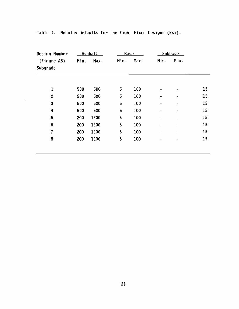
Table 1. Modulus Defaults for the Eight Fixed Designs {ksi).
Design Number {Figure AS)
Subgrade
1
2
3
4
5
6
7
8
Asohalt Min. Max.
500 500
500 500
500 500
500 500 200 1200
200 1200
200 1200
200 1200
Base Min. Max.
5 100
5 100
5 100 5 100
5 100
5 100 5 100
5 100
21
Subbase Min. Max.
15 15
15
15
15
15 15
15

The cursor moves to the second field where the program requests the surface layer material. Enter <L> for crushed limestone aggregate or <G> for crushed river gravel aggregate, and press <ENTER> to continue to the next input field. The options to be selected in this field deserve a brief explanation.
The program has built into it equations for stiffness versus temperature for typical mixes found in Texas (crushed limestone or river gravel mixes). Also equations which represent the reasonable range of stiffnesses are available. These were generated by analyzing stiffness results and obtained on rutted mixes (low stiffnesses) and badly cracked mixes (high stiffness). In the backcalculation procedure, if the user wishes to use a fixed default asphalt modulus, which is often the case on these pavements, then a single value is calculated based on the coarse aggregate type and FWD test temperature. However, if an asphalt modulus is to be backcalculated, then an acceptable range of moduli values is generated using the equation for rutted and cracked mixes, and the FWD test temperature.
This option was intended for field personnel who are familiar with materials information but who have limited experience with modulus backcalculation techniques. In this field select whether you want the program to backcalculate a fixed value or a range of values for the asphalt moduli. Enter <F> for a fixed value or <R> for a range and press <ENTER> or press <FKl> to see the formulas used for each of these two options. The last field in this screen prompts for the pavement temperature in degrees Fahrenheit. Enter the temperature value and press <ENTER>. Use the <ESC> key to return to the first field and make changes, as explained previously.
After validating the pavement temperature with a <ENTER>, the program displays a second screen {Figure 9). In this screen the user selects the material to be used for the base, subbase if any, and subgrade of the pavement sections to be analyzed. The input sequence is organized in five fields. In the first field enter any of the nine available base material options. The second field takes the base thickness in inches. If a subbase is present, input its type and thickness as for the base. Leave the subbase type blank by pressing <ENTER> if there is no subbase.
22

Enter the predominant type of subgrade for the section as per the option list. Changes to the screen can be made using the <ESC> key as described previously. Press <ENTER> to validate the input and to run the program. This time the message "The WESS Program is running ... " appears in the screen to indicate that the program is executing. When WESS is complete, the data base is generated, and the Path Search algorithm program takes over; the respective message is displayed to indicate that it is executing. Completion of the search phase is confirmed by the "Search program terminated normally!" and "Press any key to continue" messages. Pressing any key leads you to the Print Results Menu.
4.4 Option 3 - Run a Full Analysis This option of the Modulus Backcalculation Menu lets the user specify
the thickness, moduli ranges, and Poisson ratios for up to four layers within a pavement section. When you request this option, the input screen (Figure 10) is displayed. The values that are displayed on the screen are the values used in the most recent run of the program. To run the program with these values press <ENTER>. The existing values can be edited at three levels which are accessible through function keys two to four. The editing levels correspond to the degree of likelihood in which the user would change the values, from less to more likely.
For all practical purposes, information such as plate radius, number of sensors and sensor distance to the plate are prone to remain the same throughout the length of a project since these values reflect the characteristics of the FWD. At this point press the <ESC> key if you want to abort the program. Editing is done in the same way as for the previous programs; that is, you enter the desired value and validate it by pressing <ENTER>.
If you want to change all the values on the screen, press the <FK2> key. The cursor will be positioned in the plate radius field. Enter the plate radius in inches and the number of deflection sensors. Then enter the spacing of the sensors in inches and the weighing factor to be used for each sensor. For the FWD, a typical plate radius is 5.91 inches with spacings at 0, 12, 24, 36, 48, 60 and 72 inches. Note: sensors must be placed at 0, 12, 24 and 36 in MODULUS 4.0. The user may wish to assign
23

V4.0 MODULUS
<FK2> PLATE RADIUS (IN) - - - - XXXXXX
NUMBER OF SENSORS - - - X SENSOR NUMBER 1 2 3 4 5 6 7
DISTANCE FROM PLATE - XXXXXX XXXXXX XXXXXX XXXXXX XXXXXX XXXXXX XXXXXX WEIGHTING FACTOR - XXXX XXXX XXXX XXXX XXXX XXXX XXXX
HMAC SURFACE LAYER THICKNESS (IN) - - - - - - - - - - - - - - - - - XXXXX HMAC WITH CRUSHED (L)IMESTONE OR CRUSHED RIVER (G)RAVEL AGGREGATE - - - X USE A (F)IXED VALUE OR A (R)ANGE OF VALUES FOR THE ASPHALT MODULUS
BASED ON TEMPERATURE - - - - - - - - - - - - - - - - - - - - - - - - X INPUT ASPHALT TEMPERATURE (?F) - - - - - - - - - - - - - - - - - - - XXXX
Figure 8. Input Material Types.
MODULUS BASE AND SUBBASE TYPES 1) CRUSHED LIMESTONE 2) ASPHALT BASE 3) CEMENT TREATED BASE 4) LIME TREATED BASE 5) IRON ORE GRAVEL 6) IRON ORE TOPSOIL 7) RIVER GRAVEL 8) CALICHE GRAVEL 9) CALICHE
THICKNESS BASE TYPE - - - X > XXXX
SUBBASE TYPE - X > XXXX
Figure 9. Input Base and Subgrade Types.
24
V4.0
PREDOMINANT SUBGRADE TYPE 1) GRAVELLY SOILS 2) SANDY SOILS 3) SILTS 4) CLAYS, LL < 50 5) CLAYS, LL > 50
SUBGRADE TYPE - - - - - X

V4.0 MODULUS
<FK2> PLATE RADIUS (IN) - - - - - XXXXXX NUMBER OF SENSORS - - X SENSOR No. I 2 3 4 5 6 7 DIS. FROM PLATE - XXXXXXX XXXXXXX XXXXXXX XXXXXXX XXXXXXX XXXXXXX XXXXXXX WEIGHTING FACTOR XXXX xx xx xx xx
<FK3> HI LAYER THICKNESS (IN) - - - - - - XXXXX
MODULUS RANGES FOR: MINIMUM (KSI)
<FK4> SURFACE LAYER - XXXXXXXXX BASE LAYER - - - - - XXXXXXXXX SUBBASE LAYER - - - - XXXXXXXXX
xx xx xx xx xx xx xx xx
H2 xxxxx
MAXIMUM (KSI)
xxxxxxxxx xxxxxxxxx xxxxxxxxx (KSI)
H3 xxxxx
H4 xxxxx
POISSON'S RATIO xxxx xx xx xxxx
SUBGRADE MODULUS (MOST PROBABLE VALUE) - -XXXXXXXXX
POISSON'S RATIO xxxx
Figure 10. Full Analysis.
25

weight factors to each geophone or let the program assign them automatically. Leave all the weighting factors at zero for automatic assignment. However, if the user wishes to override this he simply inputs the desired weighting factors. Weighting Factors typically range from 0 to 1.0, a weighting factor of 0 will remove that sensor from the calculation process.
To change layer thicknesses and modulus ranges, press the <FKJ> key. In these four fields labelled HI to HJ, enter the pavement thicknesses in inches. HI represents the surface layer, H2 the base layer and HJ the subbase layer. The H4 value is automatically calculated and represents the depth in the pavement at which a stiff layer is calculated to occur. (See Report II23-3 for details} This may be bedrock or a stiff clay layer, for example. The user can overwrite this number if needed. Use 300 inches as the maximum possible value of H4. For a four layer pavement, enter the thicknesses in its respective fields. For a three layer system with no subbase, enter the surface thickness, the base thickness, then zero <0> to indicate the absence of subbase. For a two layer pavement, the procedure is the same except that a thickness of <0> is entered for the base layer. To change the modulus ranges only, press the <FK4> key. Enter the lower modulus boundary value, the upper boundary value, and the poisson value for the surface layer. Then, depending on whether the pavement is a two, three, or four layer system, the cursor will move to the corresponding field allowing you to edit the values for the particular layer. Next, enter the most probable modulus value in ksi and the corresponding poisson ratio value for the subgrade. After entering the value for the subgrade layer poisson ratio, check all the input values and if necessary, change any values using the appropriate function key and repeat the above process. If satisfied with the input, press <ENTER> to execute the program. The "WESS Program is Running ... " message should now appear on the screen.
When the program is complete, it displays the appropriate message and asks the user to press any key. The Print Results Menu is then displayed, and the user can obtain a printout of the analysis results.
26

CHAPTER V OPTION 3 PLOT DEFLECTION AND/OR MODULI VALUES PROGRAM
This program allows the user to analyze pavement response variables, mainly deflection readings, calculated moduli values, depth to bedrock and average errors, from a graphical point of view, along the entire project length. It will also perform a unit delineation analysis using the cumulative difference approach in order to identify units of sections having similar characteristics. {See Report 1123-1,}
To run this program select option three from the Main Program Menu and press <ENTER>. After validating the choice, the Pavement Response Variable Graphic Representation and Delineation Analysis screen is displayed {Figure 11}. Here enter the name of the data file containing both the deflection readings and the calculated moduli values for each of the pavement layers. These files are characterized by the extension .DAT in their file names; it is automatically appended to the name of the file that was specified in the backcalculation phase. Enter the file name, up to eight characters long and press <ENTER>.
Next, select the response variables to be plotted. There are a maximum of seven deflection readings and four moduli values for each station. Deflections are identified by a number from 1 to 7, 1 corresponding to the sensor closest to the loading plate, 2 to the second closest, and so on. Moduli values have labels from 8 to 11 where 8 identifies the modulus of the surface layer, 9 the base, 10 the subbase, and 11 the subgrade. Label 12 displays the absolute error and 13 shows the depth to bedrock. Enter the number corresponding to the response variable required, 1 through 7 for deflections or 8 through 11 for moduli values, 12 for absolute error or 13 for depth to bedrock, and press <ENTER>.
The last item of information requested is the minimum section length that will be used by the delineation subroutine to perform the unit delineation of the chosen response variable. If consecutive inflection points in the cumulative difference curve occur at intervals that are less than the minimum section length entered, the program will ignore them. This feature is provided to avoid the clutter of unit delineations
27

MODULUS
PAVEMENT RESPONSE VARIABLE GRAPHIC REPRESENTATION AND DELINEATION ANALYSIS
THE FOLLOWING INFORMATION IS REQUIRED:
NAME OF THE DATAFILE - - - - - - - - - - XXXXXXXX.DAT RESPONSE VARIABLE - - - - - - - - - - - XX MINIMUM SECTION LENGTH - - - - - - - - - - - - XXXXX
(C) Copyright 1989, Texas Transportation Institute. All rights Reserved
Figure 11. Setup for Graphics.
28
V4.0

that might occur in projects with unusually high response variable variability.
Enter this value in miles including fractions of a mile, that is, as a decimal value, and press <ENTER>. To make any changes, use the <ESC> sequence as in the other programs.
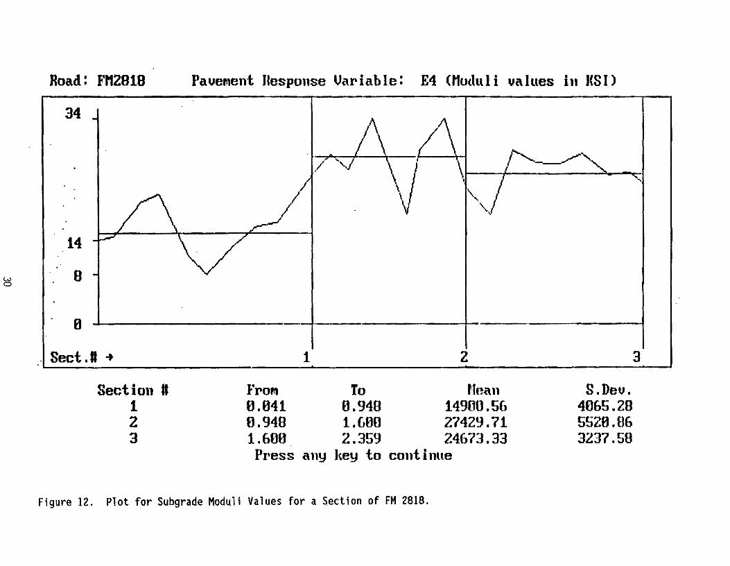
As soon as the <ENTER> key is pressed, the program starts executing, and in a few seconds, the screen is cleared, and a plot of the selected response variable as a function of distance along the project is produced (Figure 12). At the bottom of the screen a table of statistics for each of the unit delineations is displayed. If there are more than three delineated sections in the plot, press any key to see the statistics for the remaining sections. Press any key until the message "Would you like to combine sections manually or Quit? (C/Q):" appears. To quit the program at this point enter <Q>, otherwise enter <C>. The manual combination routine then prompts for the number of sections the user would like the combination to have. Enter the number and press <ENTER>. To combine all sections, enter the total number of sections that were delineated in the plot. If the user did not elect to combine all sections, a prompt is displayed asking for the number of the last section to be included as the new section one. The subroutine repeats the last prompt until all of the sections have been accounted for. Then it recalculates and replots the curve showing the new delineations and their respective statistics.
Repeat the above sequence for manual combination if there are sections left to combine or quit the program. When the user answers <Q> to the prompt, the user is given the choice of printing the statistics for the latest delineation. Then, the following prompt is displayed: "Enter <R> to analyze other Responses or <Q> to quit to the Main Program Menu:". Selecting <Q> returns to the Main Program Menu while entering <R> redisplays the Pavement Response Variable Graphic Representation and Delineation Analysis screen, allowing the user to select another response variable for graphical analysis.
29
Road: Fl12B19
34
14
B
0
. Sect .II +
Section U 1 2 3
Paue111ent Jlesponse Variable: E4 CMu<lul i ualues in }(SI)
I
1 2
l"roM To Hoa n 0.041 0.949 14900.5& 0.949 1.b00 27429.71 1.&00 2.359 24&73.33 Pr'ess any l<ey to continue
S.Deu. 40&5.29 5520.BG 3237.59
Figure 12. Plot for Subgrade Moduli Values for a Section of FM 2818.
3

CHAPTER VI PRINT RESULTS PROGRAM
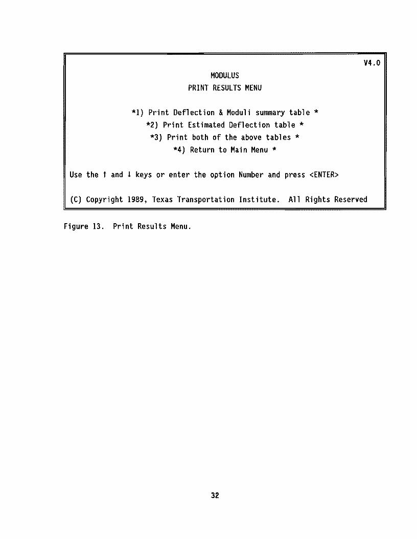
The Print Results of Latest Analysis option in the Main Program Menu give the user direct access to the same Print Results Menu {Figure 13) that is displayed after any of the three options in the Modulus Back Calculation Program terminate execution. It allows the user to print a results summary table or a detailed estimated deflection report, or both for the analysis that was performed the last time the Back Calculation program was used.
The options in this menu are:
•PRINT DEFLECTION & MODULI SUMMARY TABLE: This option lets the user print a table listing the deflection readings, the calculated moduli values, and the estimated absolute percent error per sensor for each station in the project and the estimated depth to a stiff layer for each deflection bowl. At the bottom of the figure, statistics are printed for all of the above variables (Figure 14). The asterisk printed at the end of the line denotes moduli values which hit upper or lower limits of either, the range of allowable input moduli values or modular ratios used within the program to generate the deflection data base. If more than 103 of deflection bowls hit a limit then the user should rerun the program with wider limits to eliminate this problem.
•PRINT ESTIMATED DEFLECTION TABLE: Option <2> of the Print Results Menu produces a detailed station by station result report which includes the back calculated deflection values, absolute error and squared error values, force and pressure at the loading plate, and a list of checks indicating if the moduli values are close to the given limits, if the convexity test fails, or if the solution to the particular station was infeasible {Figure 15).
•PRINT BOTH OF THE ABOVE TABLES: This option prints the summary table first, advances the paper to the beginning of a new page, and then prints the detailed section by section report.
•RETURN TO MAIN MENU: It does just that.
31
MODULUS PRINT RESULTS MENU
*l) Print Deflection & Moduli summary table * *2) Print Estimated Deflection table * *3) Print both of the above tables *
*4) Return to Main Menu *
Use the t and i keys or enter the option Number and press <ENTER>
V4.0
(C) Copyright 1989, Texas Transportation Institute. All Rights Reserved
Figure 13. Print Results Menu.
32

n1 IODVLIS IHLTSIS srsrn (SVDllf IEPOlf) (YmlH U)
---------------------------------------------------------------------------------------------------------------------------------------District: n IODULI RllGt(psll CtHlJ: 21 THcheu(l1) lhl111 lut111 11c••11tl•ad: r1211a P1n1eat: S.H %0,00I 800,0lt
lase: 11.H 1"900 11,000 · S1bbue: .... I • S1bcrde: us.so 15,0IO . .
----------·---------------------~------------------------------------------------------------------------------------------------------Lod leanrd DeUecllH (ails): Calc1l1ted l1d1ll '1l1es (lsi): Abu lite DepU lt
Shtloa (lh) It ·12 ll 14 15 II If SHF(El) US!([Z) S11B8(E3) S11BGUO DIOR/Sm. ldroct ---------------------------------------------------------------------------------------------------------------------------------------
I.OH u,m 31.H %1.U 1%.%5 r.u 5.H Ut z.u 108. U.9 ••• 1.2 2.U 2U.U I
1.104 11,tn u.n 11.H 10.%8 '· 75
UC 3.U tn uo. 25.9 ••• u.o 1.55 300.00 I
t.%14 u,m JI.IT u.u t. 45 (.tf us 2.U l.U sos. U.t ••• U.I I.SI Ul.U t.%95 U,4U U.H 20. 70 1.59 4.'1 J.2t 2.4& 2.11 SU. 13.7 I.I U.2 1.35 JOI.IS 1.m u,m 44.33 U.32 lS.50 I.It 5. 77 (.ti s.u TOO. u.o ••• f.I 1.32 144.U 1
1.501 11,on U.%0 31.'5 U.73 11.U 1.0 5.39 4.54 no. 10.3 ••• 5.% 1.91 1$7.08 e.sot ll,111 34.21 %1.U ll.U 7.IO S.34 3.17 l.17 . uo. 33.9 1.0 I.I %.ID %3%.12 •• 708 1%,111 u.a U.45 11.10 s.u t.H 1.21 z.u HO. 39.1 ••• '·' t.n 2J0, 2J I
t.103 11,m u.n 11.u I.St S.15 tlS s.u t.33 IOO. 11.1 ••• U.8 n.u UZ.J3 I
e.tu 11,lU u.u u.u s.u J.U 2.JT 1.n t.U 117. 15.J ••• U.1 1.18 U.11
··-----------------------------------·----------------------------------------------------------------------·--------------------------lu1: H.U 21.U U.37 I.IS 4.12 3.35 2.75 518. 2T •• ••• U.5 4.71 159.U SIL Du: lt.35 f.U Ut Z.15 1.U l.U . 1.11 uz. U.J ••• ts T.U u.u Tar Coe U (II: u.n JC.ti JS.SS H.%5 U.H JI.TT u.ss SS. H.I ••• JJ.4 m.u 43.0S
---------------------------------------------------------------------------·-----------------------------------------------------------
Figure 14. Summary Listing.
33
\

Page: 1
TTl IODULUS AKALJSIS StSTEI (SECTIOI REPORT) (YmlH U)
District: 17 Co1nty: 21 Blc•r17/R•ad: Flt318
Dlsta1ce (ia) fro1 ceater of loading plate to seasor: it = UDO U.OOI ZC.001 JS.000 41.000 U.000 n.ooo
l1di1s of loadi1g plate(inl: 5.UO 3.000
10. 000 uoo
uuoo
S1rf1ce t\ictaess(ln): lase tilctness(in): Sa•base tllciaess(ln): Sabgrade tllctness(ln):
Shlioa: 0.041 leisured Dtflectlo1: C1lc1lated Deflectlo1: leicit Factor:
I ERROR L11er: lod1ll him (lsi ): Cltse to llails!
Shlloa: O.U4 leas1red Deflection: C1lc1late• Detlectioa: leicU factor:
S EIROR La1er: le41ll Valtes (tsl): Close to llaits!
Shtloa: UH leasared Deflecll11: Calc1laled Defleclioa: leicbt Factor:
I ERROR L17er: 1•••11 f1J1es (lsi): Clise to llalts!
Sh tin: o.m le1s1red Deflection: Calc1late• Deflectlo1: leigit Factor:
S t:llOR Later: lei1ll Yalies (ksl): Close to liaits!
RI lo.GO 31.33 1.00
-%.40 SDIUCE(El)
800.0 TES
It tU9 40.U 1.H 1.28
SURFACE([!) %00.0 JES
Rt JS.OT ll.01 1.00 0.11
SURUCE(Ell m.o 10
11 3UC to.OD LOO
·O.tD SDIFACE(El I
585.8 110
12 RJ u.u u.zs 20.31 12.U us 0.H 3.85 1.50
umm 3U 10
IU u 11.34 10.%1 19.U 9.14 1.41 o.u
-tUS uo BASE(E%1 zu 10
12 u 19.U 9. ($
20.0S 9.%1 o.u o.u
-0.7t 2.n umm JC.4 10
IZ u 2D.7D 1.51 20.SC 8.U 1.52 D.%1 o.u -0.Cl
IASE{E2)
U.7 IO
POISSON RATIO YALUES Bl: J : us U: ' = 0.30 IJ: ' : t.30 14: ' : 1.40
R4 RS T.U s.ac 1.15 5.0C 0.24 0.01
-3.&0 D.00
IS 3.51 3.U O.Of 1.00
SUBB!SE(El) SUBGRADE(Et) 0.0 u
N/A
RI as RS 1.75 UC 3.65 5.15 UC 2.U 0.1C 0.00 0.01
13.l7 0.01 O.Dt SllBBASEIEll SUBGUDE (E4)
t.O ll.O NIA
Kt 85 RS c.n l.U 2.%1 5.11 3.17 z.ot 0.13 0.01 O.OI
-z.u 0.00 1.00 sum mm SUBGUDE(EO
u 11.8 I/A
14 15 H Ut U4 %.H c.u 2.15 LU 1.1% 0.00 0.00 O.H l.01 0.08
SOBBASE([l) SDBGBADE(Et) I.I tu
I/A
RT z.u 2.%7 0.18 1.00
Rf %.91 1.50 o. 00 0.00
R1 1.11 1.U O.OI ....
If %.DI l.U 0.00 O.Ot
1% : ll = U= 15 : IC = Rt :
Plate Lod = 11,m Ih Phte Pmure = m.m psi
Absolale S11 of S ERROR = 10.300 Squ re Err or = O.OOl
Failed Ct1Ye1itJ Test! 10
Plate Load = u,m as Plate Press1re = 108.410 psi
A•sol1te S11 of S ERROi : u.m Squre Ernr = o.m
Failed Coa•exitJ Test! ID
Plate Load = 11,m th Plate Press1re = 10l.S8t psi
A•sol1te S11 of S ERROR = c.m S•ure Error = t.otz
Faile• Ct1Ye1lt1 Test! 10
Plate Lod = 12,m l)s Plate Pre1s1re = 113.?30 psi
i•sol1le S11 of S ERROR = 1.411 Squre Errn = uoo
Failed C11Yesit7 Test! 10 ------······---------------------------------------------~---------------------------------------------------------···---------------~-
Station: •.m 11 u R3 u 15 B6 Rf Plate Lu~ = 11,m us le1s1red Deflectl11: 44.33 28.lt 15.51 I.II 5.7? 4.U 3.15 Plate Press1re = 104.Jtt psi Calc1l1ted Deflecti11: 4U4 %8.10 1$.%3 I.SS 5.H 3.70 %.tt leigbt F1clor: 1.at O.H 0.3$ o. %0 1.80 o.oo O.H
I EIROR ·1.70 0.19 1. 71 -%.01 0.00 O.OI 0.00 Absol1te S11 of S ERROR = 5.m Lay'r: sommrn umm susumm SUBGUD£(EO S~ure Error = t.OOl ltd1li Yalies (tsJ): TOG.2 11.0 ••• r.. Clise It ll1lts! JES IO Iii Fallec Ct1Ye1itJ Test! 10
---------------------··--·----------·------------------------------*---------------------------------------------------------~---·---~~
Figure 15. Detailed Bowl by Bowl listing.
34

CHAPTER VII CUSTOMIZING FIXED DESIGNS
The first option in the Modulus Backcalculation menu, "Use an Existing Fixed Design", allows the user to access 24 different design types that are characteristic of Texas. These are divided into three groups: fixed designs one through eight, nine through 16, and 17 through 24 that differ from each other in the depth to bedrock and type of subgrade assumed. Designs one through eight assume a SAND subgrade and depth to bedrock of 120 inches, designs nine through 16 are for a sandy/clay with a 180 inch depth to bedrock and designs 17 through 24 assume a CLAY subgrade and a 240 inch depth to bedrock.
The process for creating fixed designs is straight forward and includes three steps:
•Running the "Full Design" option from the Modulus Backcalculation Menu using the parameters for the new fixed design; •Renaming the TMP.DEF and WES.RES files produced in the previous step to TMP#.DEF and WES#.RES respectively, where # stands for the number of the existing fixed design being replaced; and eModifying the DESIGNS.DAT file which stores the fixed design menu definitions to reflect the change.
The above procedure has to be duplicated every time a new fixed design is to be incorporated into the system. To replace a new design it is recommended that the new design be new for all three depths to bedrocks (240", 180 11
, and 120"} to include the clay, sandy/clay and sand subgrade types. For example TMPI.DEF and WESI.RES (120"), TMP9.DEF and WES9.RES{l80"), and TMP17.DEF and WES17.RES (240 11
) contain information for pavement type 1 of the fixed design option. Replace all of these files with the output from the modulus backcalculation and change the appropriate entry in the DESIGNS.DAT file to reflect the layer thicknesses and layer material types of the new fixed design you have created.
Note: The system should be backed up regularly.
35