Embed Size (px)
Citation preview

2 Forecasting logistics requirements
2.1 Introduction2.2 Qualitative methods2.3 Quantitative methods2.4 Data preprocessing2.5 Choice of the forecasting method2.6 Advanced forecasting method2.7 Accuracy measure and forecasting monitoring2.8 Interval forecasts2.9 Case study: Forecasting methods at Adriatica Accumulatori
2.10 Case study: Sales forecasting at Orlea2.11 Questions and problems
G. Ghiani, G. Laporte, R. Musmanno Introduction to Logistics System Management © John Wiley & Sons, Ltd 1 / 31
2 Forecasting logistics requirements Accuracy measure and forecasting monitoring
Introduction (1/2)
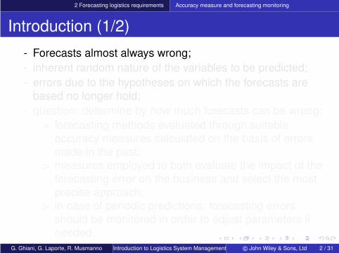
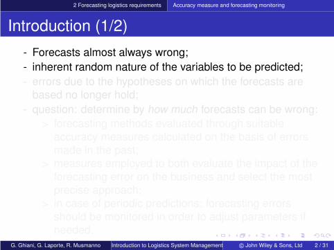
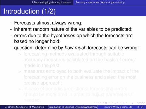
- Forecasts almost always wrong;- inherent random nature of the variables to be predicted;- errors due to the hypotheses on which the forecasts are
based no longer hold;- question: determine by how much forecasts can be wrong:
> forecasting methods evaluated through suitableaccuracy measures calculated on the basis of errorsmade in the past;
> measures employed to both evaluate the impact of theforecasting error on the business and select the mostprecise approach;
> in case of periodic predictions: forecasting errorsshould be monitored in order to adjust parameters ifneeded.
G. Ghiani, G. Laporte, R. Musmanno Introduction to Logistics System Management © John Wiley & Sons, Ltd 2 / 31
2 Forecasting logistics requirements Accuracy measure and forecasting monitoring
Introduction (1/2)
- Forecasts almost always wrong;- inherent random nature of the variables to be predicted;- errors due to the hypotheses on which the forecasts are
based no longer hold;- question: determine by how much forecasts can be wrong:
> forecasting methods evaluated through suitableaccuracy measures calculated on the basis of errorsmade in the past;
> measures employed to both evaluate the impact of theforecasting error on the business and select the mostprecise approach;
> in case of periodic predictions: forecasting errorsshould be monitored in order to adjust parameters ifneeded.
G. Ghiani, G. Laporte, R. Musmanno Introduction to Logistics System Management © John Wiley & Sons, Ltd 2 / 31

2 Forecasting logistics requirements Accuracy measure and forecasting monitoring
Introduction (2/2)
- case of a regular time series;- one-period-ahead forecast.
G. Ghiani, G. Laporte, R. Musmanno Introduction to Logistics System Management © John Wiley & Sons, Ltd 3 / 31

2 Forecasting logistics requirements Accuracy measure and forecasting monitoring
Introduction (2/2)
- case of a regular time series;- one-period-ahead forecast.
G. Ghiani, G. Laporte, R. Musmanno Introduction to Logistics System Management © John Wiley & Sons, Ltd 3 / 31

2 Forecasting logistics requirements Accuracy measure and forecasting monitoring
Accuracy measures (1/7)Mean absolute deviation (MAD) at time period T (> 1):
MADT =
T∑
t=2|et |
T −1; (1)
Mean absolute percentage deviation (MAPD) at time period T(> 1):
MAPDT =
T∑
t=2
|et |yt
T −1; (2)
Mean squared error (MSE)) at time period T (> 2):
MSET =
T∑
t=2e2
t
T −2. (3)
G. Ghiani, G. Laporte, R. Musmanno Introduction to Logistics System Management © John Wiley & Sons, Ltd 4 / 31

2 Forecasting logistics requirements Accuracy measure and forecasting monitoring
Accuracy measures (2/7)
- Used at time period t =T to establish a comparisonbetween different forecasting methods;
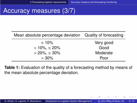
- MAPD used to evaluate the quality of a forecasting method(see Table 1).
G. Ghiani, G. Laporte, R. Musmanno Introduction to Logistics System Management © John Wiley & Sons, Ltd 5 / 31

2 Forecasting logistics requirements Accuracy measure and forecasting monitoring
Accuracy measures (2/7)
- Used at time period t =T to establish a comparisonbetween different forecasting methods;
- MAPD used to evaluate the quality of a forecasting method(see Table 1).
G. Ghiani, G. Laporte, R. Musmanno Introduction to Logistics System Management © John Wiley & Sons, Ltd 5 / 31
2 Forecasting logistics requirements Accuracy measure and forecasting monitoring
Accuracy measures (3/7)
Mean absolute percentage deviation Quality of forecasting
≤ 10% Very good> 10%, ≤ 20% Good> 20%, ≤ 30% Moderate
> 30% Poor
Table 1: Evaluation of the quality of a forecasting method by means ofthe mean absolute percentage deviation.
G. Ghiani, G. Laporte, R. Musmanno Introduction to Logistics System Management © John Wiley & Sons, Ltd 6 / 31

2 Forecasting logistics requirements Accuracy measure and forecasting monitoring
Accuracy measures (4/7)
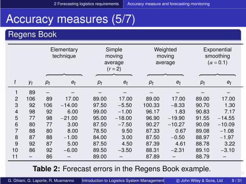
Regens BookWe want to assess the accuracy of the elementary technique, ofthe moving average (with r = 2), of the weighted moving averageand of exponential smoothing (α= 0.1) methods in the RegensBook example, introduced in Section 2.5.4.1. The results of thefour forecasting methods are reported in Table 2. On the basisof the accuracy measures shown in Table 3, we can state that allthe methods provide good-quality forecasts. In particular, themost accurate technique turned out to be the exponentialsmoothing method (with α= 0.1).
G. Ghiani, G. Laporte, R. Musmanno Introduction to Logistics System Management © John Wiley & Sons, Ltd 7 / 31
2 Forecasting logistics requirements Accuracy measure and forecasting monitoring
Accuracy measures (5/7)Regens Book
Elementary Simple Weighted Exponentialtechnique moving moving smoothing
average average (α= 0.1)(r = 2)
︷ ︸︸ ︷ ︷ ︸︸ ︷ ︷ ︸︸ ︷ ︷ ︸︸ ︷
t yt pt et pt et pt et pt et
1 89 – – – – – – – –2 106 89 17.00 89.00 17.00 89.00 17.00 89.00 17.003 92 106 −14.00 97.50 −5.50 100.33 −8.33 90.70 1.304 98 92 6.00 99.00 −1.00 96.17 1.83 90.83 7.175 77 98 −21.00 95.00 −18.00 96.90 −19.90 91.55 −14.556 80 77 3.00 87.50 −7.50 90.27 −10.27 90.09 −10.097 88 80 8.00 78.50 9.50 87.33 0.67 89.08 −1.088 87 88 −1.00 84.00 3.00 87.50 −0.50 88.97 −1.979 92 87 5.00 87.50 4.50 87.39 4.61 88.78 3.22
10 86 92 −6.00 89.50 −3.50 88.31 −2.31 89.10 −3.1011 – 86 – 89.00 – 87.89 – 88.79 –
Table 2: Forecast errors in the Regens Book example.G. Ghiani, G. Laporte, R. Musmanno Introduction to Logistics System Management © John Wiley & Sons, Ltd 8 / 31

2 Forecasting logistics requirements Accuracy measure and forecasting monitoring
Accuracy measures (6/7)
Regens Book
Elementary Simple Weighted Exponentialtechnique moving moving smoothing
average average (α= 0.1)(r = 2)
MAD10 9.00 7.72 7.27 6.61MAPD10 10.12% 8.78% 8.30% 7.43%MSE10 137.13 104.03 111.31 85.08
Table 3: Accuracy values of the forecasting methods used by RegensBook.
G. Ghiani, G. Laporte, R. Musmanno Introduction to Logistics System Management © John Wiley & Sons, Ltd 9 / 31

2 Forecasting logistics requirements Accuracy measure and forecasting monitoring
Accuracy measures (7/7)
Rule of thumbA forecasting method made on a sporadic time series isaccurate if its MAPD is less than 30%.
G. Ghiani, G. Laporte, R. Musmanno Introduction to Logistics System Management © John Wiley & Sons, Ltd 10 / 31

2 Forecasting logistics requirements Accuracy measure and forecasting monitoring
Tuning of the forecasting methods (1/5)- Accuracy measures used to tune the forecasting methods
depending on one or more parameters (like exponentialsmoothing and Winters techniques);
- basic idea: assign the parameters the values that wouldhave maximized the accuracy of the forecasts in the past.
Example. By using the mean squared error, the mostsuitable parameter α∗ of the exponential smoothing methodat time period T can be determined as the solution of theoptimization problem:
MinimizeMSET (α)
subject to0≤α≤ 1.
G. Ghiani, G. Laporte, R. Musmanno Introduction to Logistics System Management © John Wiley & Sons, Ltd 11 / 31

2 Forecasting logistics requirements Accuracy measure and forecasting monitoring
Tuning of the forecasting methods (2/5)
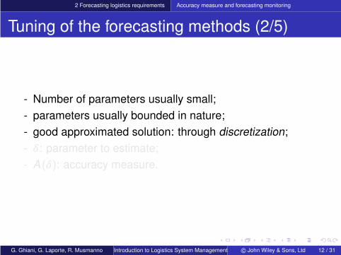
- Number of parameters usually small;- parameters usually bounded in nature;- good approximated solution: through discretization;- δ: parameter to estimate;- A(δ): accuracy measure.
G. Ghiani, G. Laporte, R. Musmanno Introduction to Logistics System Management © John Wiley & Sons, Ltd 12 / 31

2 Forecasting logistics requirements Accuracy measure and forecasting monitoring
Tuning of the forecasting methods (2/5)
- Number of parameters usually small;- parameters usually bounded in nature;- good approximated solution: through discretization;- δ: parameter to estimate;- A(δ): accuracy measure.
G. Ghiani, G. Laporte, R. Musmanno Introduction to Logistics System Management © John Wiley & Sons, Ltd 12 / 31

2 Forecasting logistics requirements Accuracy measure and forecasting monitoring
Tuning of the forecasting methods (3/5)
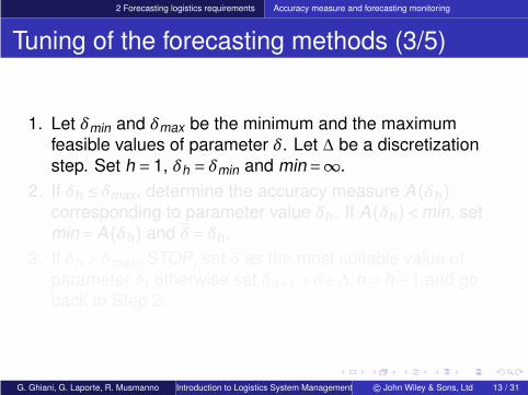
1. Let δmin and δmax be the minimum and the maximumfeasible values of parameter δ. Let ∆ be a discretizationstep. Set h = 1, δh = δmin and min=∞.
2. If δh ≤ δmax, determine the accuracy measure A(δh)corresponding to parameter value δh. If A(δh)<min, setmin=A(δh) and δ= δh.
3. If δh > δmax, STOP, set δ as the most suitable value ofparameter δ, otherwise set δh+1 = δ+∆,h = h+1 and goback to Step 2.
G. Ghiani, G. Laporte, R. Musmanno Introduction to Logistics System Management © John Wiley & Sons, Ltd 13 / 31

2 Forecasting logistics requirements Accuracy measure and forecasting monitoring
Tuning of the forecasting methods (3/5)
1. Let δmin and δmax be the minimum and the maximumfeasible values of parameter δ. Let ∆ be a discretizationstep. Set h = 1, δh = δmin and min=∞.
2. If δh ≤ δmax, determine the accuracy measure A(δh)corresponding to parameter value δh. If A(δh)<min, setmin=A(δh) and δ= δh.
3. If δh > δmax, STOP, set δ as the most suitable value ofparameter δ, otherwise set δh+1 = δ+∆,h = h+1 and goback to Step 2.
G. Ghiani, G. Laporte, R. Musmanno Introduction to Logistics System Management © John Wiley & Sons, Ltd 13 / 31

2 Forecasting logistics requirements Accuracy measure and forecasting monitoring
Tuning of the forecasting methods (4/5)
Regens BookWe want to tune the exponential smoothing method for theRegens Book problem, by utilizing the mean absolute deviationas an accuracy measure.By using αmin = 0, αmax = 1 and ∆= 0.1, we get the deviationsreported in Table 4. On the basis of these results, the mostsuitable value of the forecasting parameter is α= 0.2.
G. Ghiani, G. Laporte, R. Musmanno Introduction to Logistics System Management © John Wiley & Sons, Ltd 14 / 31

2 Forecasting logistics requirements Accuracy measure and forecasting monitoring
Tuning of the forecasting methods (5/5)
Regens Book
α MAD10(α) α MAD10(α)
0.0 6.56 0.6 7.640.1 6.61 0.7 7.800.2 6.42 0.8 7.910.3 6.65 0.9 8.260.4 7.07 1.0 9.000.5 7.40
Table 4: Mean absolute deviations MAD10(α) corresponding tovarious α values in the Regens Book problem.
G. Ghiani, G. Laporte, R. Musmanno Introduction to Logistics System Management © John Wiley & Sons, Ltd 15 / 31

2 Forecasting logistics requirements Accuracy measure and forecasting monitoring
Forecast control
- A forecasting method works correctly if the errors arerandom and not systematic;
- typical systematic errors occur when the variable to bepredicted is constantly underestimated or overestimated, ora seasonal variation is not taken into account;
- forecast control:> aims at identifying systematic errors in periodic
predictions (caused e.g. by a shift in trend) in order toadjust parameters if needed;
> done through a tracking signal or a control chart.
G. Ghiani, G. Laporte, R. Musmanno Introduction to Logistics System Management © John Wiley & Sons, Ltd 16 / 31

2 Forecasting logistics requirements Accuracy measure and forecasting monitoring
Tracking signal (1/7)
- KT at time period T (T > 1): ratio between the cumulativeerror at time period T and MADT
KT =
T∑
t=2et
MADT;
- greater than zero: systematic underestimate of the datumentry;
- negative value: systematic overestimate of the datum entry.
G. Ghiani, G. Laporte, R. Musmanno Introduction to Logistics System Management © John Wiley & Sons, Ltd 17 / 31

2 Forecasting logistics requirements Accuracy measure and forecasting monitoring
Tracking signal (2/7)
- Unbiased forecast: if KT falls in the range of ±K ;- value of K established heuristically (usually between 2 and
5);- if KT outside this interval: parameters of the forecasting
method modified or different forecasting method selected;- KT also used as a different accuracy measure of a
forecasting method.
G. Ghiani, G. Laporte, R. Musmanno Introduction to Logistics System Management © John Wiley & Sons, Ltd 18 / 31

2 Forecasting logistics requirements Accuracy measure and forecasting monitoring
Tracking signal (3/7)
PlazaThree months ago, the logistician of the supermarket chainPlaza (in Bolivia) was in charge of devising and monitoringmonthly forecasts for the company’s sportswear items. Thesales of the previous 12 months (in k$) are reported in Table 5.After a preliminary study of the time series, he decided to makeuse of the exponential smoothing method. The optimalsmoothing parameter α was obtained by minimizing MAD12(α).The corresponding solution was α∗ = 0.26 which was associatedwith MAD12(α
∗)= 15.95. The forecasts pt , t = 2, . . . ,12, arereported in the third column of Table 5.
G. Ghiani, G. Laporte, R. Musmanno Introduction to Logistics System Management © John Wiley & Sons, Ltd 19 / 31

2 Forecasting logistics requirements Accuracy measure and forecasting monitoring
Tracking signal (4/7)
Plaza
Month Sales Forecast Month Sales Forecast
1 977 – 7 948 968.002 958 977.00 8 996 962.763 989 972.01 9 955 971.484 966 976.47 10 959 967.155 956 973.72 11 960 965.026 965 969.07 12 988 963.70
Table 5: Monthly sales of sportsware (in k$) in the Plaza problem andthe corresponding exponential smoothing forecasts with α= 0.26.
G. Ghiani, G. Laporte, R. Musmanno Introduction to Logistics System Management © John Wiley & Sons, Ltd 20 / 31

2 Forecasting logistics requirements Accuracy measure and forecasting monitoring
Tracking signal (5/7)
PlazaHence, the manager verified that the tracking signal K12 was inthe range [−4,4] (K12 =−1.65). Then, he devised the forecast forthe next month p13 = $ 970.08 k.For the subsequent month (T = 13), the sales turned out to beequal to y13 = $ 1024 k. The associated tracking signal valuewas K13 = 1.44, while the new forecast was p14 = $ 984.22 k.
G. Ghiani, G. Laporte, R. Musmanno Introduction to Logistics System Management © John Wiley & Sons, Ltd 21 / 31
2 Forecasting logistics requirements Accuracy measure and forecasting monitoring
Tracking signal (6/7)
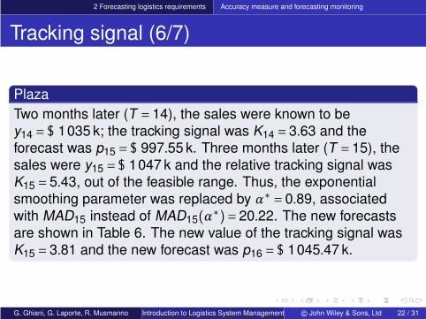
PlazaTwo months later (T = 14), the sales were known to bey14 = $ 1035 k; the tracking signal was K14 = 3.63 and theforecast was p15 = $ 997.55 k. Three months later (T = 15), thesales were y15 = $ 1047 k and the relative tracking signal wasK15 = 5.43, out of the feasible range. Thus, the exponentialsmoothing parameter was replaced by α∗ = 0.89, associatedwith MAD15 instead of MAD15(α
∗)= 20.22. The new forecastsare shown in Table 6. The new value of the tracking signal wasK15 = 3.81 and the new forecast was p16 = $ 1045.47 k.
G. Ghiani, G. Laporte, R. Musmanno Introduction to Logistics System Management © John Wiley & Sons, Ltd 22 / 31

2 Forecasting logistics requirements Accuracy measure and forecasting monitoring
Tracking signal (7/7)Plaza
Month Sales Forecast Month Sales Forecast
1 977 – 9 955 990.842 958 977.00 10 959 959.003 989 960.12 11 960 959.004 966 985.78 12 988 959.895 956 968.21 13 1024 984.866 965 957.36 14 1035 1 019.637 948 964.15 15 1047 1 033.298 996 949.80
Table 6: Monthly sales of sportsware (in k$) during the first 14 monthsin the Plaza problem and the corresponding exponential smoothingforecasts (with α= 0.89).
G. Ghiani, G. Laporte, R. Musmanno Introduction to Logistics System Management © John Wiley & Sons, Ltd 23 / 31

2 Forecasting logistics requirements Accuracy measure and forecasting monitoring
Control charts (1/8)
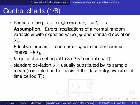
- Based on the plot of single errors et , t = 2, . . . ,T .- Assumption. Errors: realizations of a normal random
variable E with expected value µE and standard deviationσE .
- Effective forecast: if each error et is in the confidenceinterval ±kσE ;
- k : quite often set equal to 3 (‘3-σ’ control chart);- standard deviation σE : usually substituted by its sample
mean (computed on the basis of the data entry available attime period T ):
SE =
√√√√√
T∑
t=2
(
et −E)2
T −2. (4)
G. Ghiani, G. Laporte, R. Musmanno Introduction to Logistics System Management © John Wiley & Sons, Ltd 24 / 31

2 Forecasting logistics requirements Accuracy measure and forecasting monitoring
Control charts (1/8)
- Based on the plot of single errors et , t = 2, . . . ,T .- Assumption. Errors: realizations of a normal random
variable E with expected value µE and standard deviationσE .
- Effective forecast: if each error et is in the confidenceinterval ±kσE ;
- k : quite often set equal to 3 (‘3-σ’ control chart);- standard deviation σE : usually substituted by its sample
mean (computed on the basis of the data entry available attime period T ):
SE =
√√√√√
T∑
t=2
(
et −E)2
T −2. (4)
G. Ghiani, G. Laporte, R. Musmanno Introduction to Logistics System Management © John Wiley & Sons, Ltd 24 / 31

2 Forecasting logistics requirements Accuracy measure and forecasting monitoring
Control charts (2/8)
- Expected error E: equal to 0 in case there are nosystematic errors;
- (4) becomes:
SE ≈
√√√√√
T∑
t=2(et −0)2
T −2=
√
MSET ; (5)
- in case E is significantly different from 0: forecast is biased(see Figure 1);
- updating of parameters of the forecasting method (or,eventually, changing it with a more appropriate one).
G. Ghiani, G. Laporte, R. Musmanno Introduction to Logistics System Management © John Wiley & Sons, Ltd 25 / 31

2 Forecasting logistics requirements Accuracy measure and forecasting monitoring
Control charts (3/8)
0
et
t
Figure 1: Visual examination of the control chart: error with a samplemean not equal to 0.
G. Ghiani, G. Laporte, R. Musmanno Introduction to Logistics System Management © John Wiley & Sons, Ltd 26 / 31

2 Forecasting logistics requirements Accuracy measure and forecasting monitoring
Control charts (4/8)
Useful to verify visually whether the error pattern reveals thepossibility of improving the forecast by introducing suitablemodifications:
1. error pattern shows a positive or negative trend; accuracy offorecasting method progressively diminishing;
2. error pattern is periodic; an existing seasonal effect notidentified.
G. Ghiani, G. Laporte, R. Musmanno Introduction to Logistics System Management © John Wiley & Sons, Ltd 27 / 31

2 Forecasting logistics requirements Accuracy measure and forecasting monitoring
Control charts (5/8)
SoftlineSoftline, a company manufacturing leather sofas, uses themoving average method to forecast (r = 2) the monthly unitproduction cost (assuming sales volume is constant) of its topproduct called Trinity. To assess the forecasting process, thelogistician uses a ‘3-σ’ control chart. Table 7 reports the unitproduction costs as well as the forecasts and the errors madeduring the past two years. The corresponding sample meanerror was
E =e 1.40.
G. Ghiani, G. Laporte, R. Musmanno Introduction to Logistics System Management © John Wiley & Sons, Ltd 28 / 31

2 Forecasting logistics requirements Accuracy measure and forecasting monitoring
Control charts (6/8)
Softline
t yt pt et t yt pt et
1 452.00 – – 13 468.50 458.90 9.602 463.50 452.00 11.50 14 462.00 465.65 −3.653 478.00 457.75 20.25 15 470.00 465.25 4.754 466.50 470.75 −4.25 16 473.80 466.00 7.805 457.00 472.25 −15.25 17 472.00 471.90 0.106 465.20 461.75 3.45 18 478.00 472.90 5.107 460.00 461.10 −1.10 19 468.40 475.00 −6.608 457.50 462.60 −5.10 20 473.40 473.20 −0.209 463.50 458.75 4.75 21 468.00 470.90 −2.90
10 456.00 460.50 −4.50 22 463.00 470.70 −7.7011 455.00 459.75 −4.75 23 470.50 465.50 5.0012 462.80 455.50 7.30 24 475.00 466.75 8.25
25 – 472.75 –
Table 7: Unit production costs, forecasts and errors (in e) in theSoftline problem.
G. Ghiani, G. Laporte, R. Musmanno Introduction to Logistics System Management © John Wiley & Sons, Ltd 29 / 31
2 Forecasting logistics requirements Accuracy measure and forecasting monitoring
Control charts (7/8)
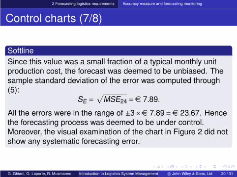
SoftlineSince this value was a small fraction of a typical monthly unitproduction cost, the forecast was deemed to be unbiased. Thesample standard deviation of the error was computed through(5):
SE =√
MSE24 =e 7.89.
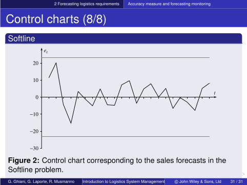
All the errors were in the range of ±3×e 7.89=e 23.67. Hencethe forecasting process was deemed to be under control.Moreover, the visual examination of the chart in Figure 2 did notshow any systematic forecasting error.
G. Ghiani, G. Laporte, R. Musmanno Introduction to Logistics System Management © John Wiley & Sons, Ltd 30 / 31
2 Forecasting logistics requirements Accuracy measure and forecasting monitoring
Control charts (8/8)
Softline
−30
−20
−10
0
10
20
et
t
Figure 2: Control chart corresponding to the sales forecasts in theSoftline problem.G. Ghiani, G. Laporte, R. Musmanno Introduction to Logistics System Management © John Wiley & Sons, Ltd 31 / 31