Embed Size (px)
Citation preview
2 Eddy Current Theory
2.1 Eddy Current Method
2.2 Impedance Measurements
2.3 Impedance Diagrams
2.4 Test Coil Impedance
2.5 Field Distributions

2.1 Eddy Current Method

Eddy Current Penetration Depth
0 ( ) i tyE F x e E e
0 ( ) i tzH F x e H e
δ standard penetration depth
/ /( ) x i xF x e e
aluminum (σ = 26.7 106 S/m or 46 %IACS)
-0.2
0
0.2
0.4
0.6
0.8
1
0 1 2 3Depth [mm]
Re
F
f = 0.05 MHz f = 0.2 MHz f = 1 MHz
f = 0.05 MHz f = 0.2 MHz f = 1 MHz
-0.2
0
0.2
0.4
0.6
0.8
1
0 1 2 3Depth [mm]
| F |
1
f
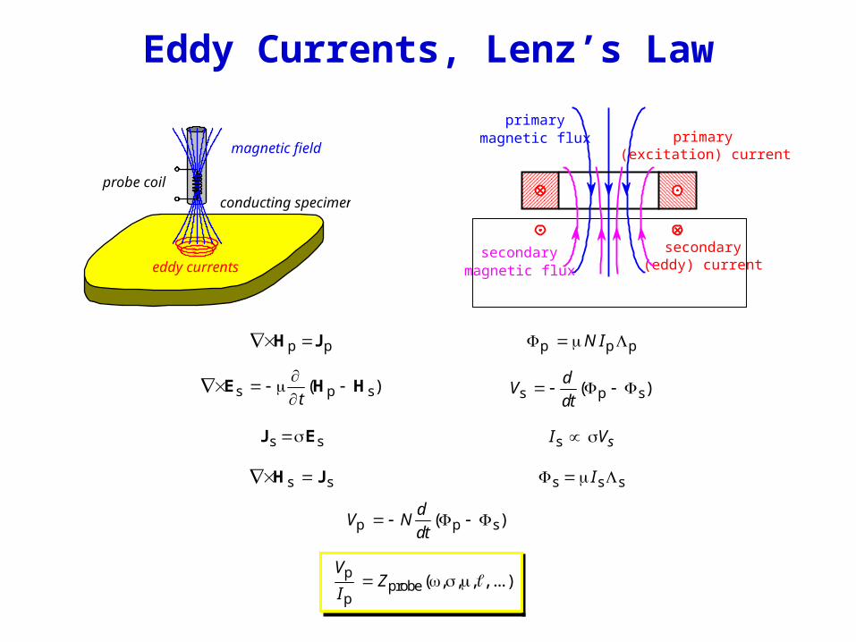
Eddy Currents, Lenz’s Law
conducting specimen
eddy currents
probe coil
magnetic field
s p s( )d
Vdt
p p H J
s p s( )t
E H H
s sJ E
p p pN I
s sI V
s s sI s s H J
secondary(eddy) current
(excitation) currentprimarymagnetic flux
primary
magnetic fluxsecondary
p p s( )d
V Ndt
pprobe
p( , , , , ... )
VZ
I

2.2 Impedance Measurements

Impedance Measurements
pI p
e
( )( )
( )
VK Z
I
Ie VpZp
Ve
Ze
VpZp
Voltage divider:
Current generator:
Iep p
Ve e p
( )( )
( )
V ZK
V Z Z
Ve p
V
( )
1 ( )
KZ Z
K

Resonance
Ve
R
L VoC
0
0.2
0.4
0.6
0.8
1
0 1 2 3Normalized Frequency,
Tra
nsfe
r F
unct
ion,
| K
|
Q = 2
Q = 5
Q = 10
p 2( )
1
i LZ
LC
po
e p
( )( )( )
( ) ( )
ZVK
V R Z
2/
( )1 /
i L RK
i L R LC
2 2( )
1 /
iQ
Ki
Q
1
LC
C RQ R R C
L L
o 21
14Q
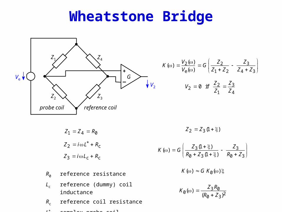
Wheatstone Bridge
32 2
e 1 2 4 3
( )( )
( )
ZV ZK G
V Z Z Z Z
Ve
V2
Z1 Z4
Z2 Z3
+
_ G32
21 4
0 ifZZ
VZ Z
1 4 0Z Z R
*2 cZ i L R
3 c cZ i L R
R0 reference resistance
Lc reference (dummy) coil inductance
Rc reference coil resistance
L* complex probe coil inductance
2 3 (1 )Z Z
probe coil reference coil
3 3
0 3 0 3
(1 )( )
(1 )
Z ZK G
R Z R Z
0( ) ( )K G K
3 00 2
0 3( )
( )
Z RK
R Z

Impedance Bandwidth
3 c cZ i L R
R0 = 100 Ω, Rc = 10 Ω
0( ) ( )K G K
3 00 2
0 3( )
( )
Z RK
R Z
0 1 2 30
0.1
0.2
0.3
0.4
0.5
Frequency [MHz]
Tra
nsfe
r F
unct
ion,
| K
0 |
Lc = 100 µH Lc = 20 µH
Lc = 10 µH
c 00 2
c 0
/( )
1 ( / )
L RK
L R
3 cZ i L
0p
c
R
L
0 p1
( )2
K
02
c
2 R
L
0 1,22
( )5
K
01
c2
R
L
2
14
2 1
c 2 1
62 or 120%
5rB
B
( , , , ,...)
2.3 Impedance Diagrams

Examples of Impedance Diagrams
Im(Z)
Re(Z)
L
C
Im(Z)
Re(Z)0
Ω-
Ω+
∞
L
C
R 0
Ω-
Ω+
∞R
Im(Z)
Re(Z)
R
L
C
0 Ω
∞ R
Im(Z)
Re(Z)
R2
L
C
0 Ω
∞ R1 R1+R2
R1
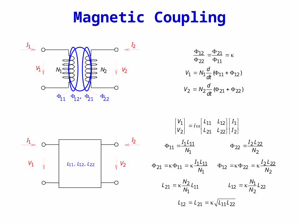
Magnetic Coupling
12 21
22 11
2 2 21 22( )d
V Ndt
1 1 11 12( )d
V Ndt
1 11 12 1
2 21 22 2
V L L Ii
V L L I
12 21 11 22L L L L
221 11
1
NL L
N 1
12 222
NL L
N
1 1121 11
1
I L
N 2 22
12 222
I L
N
1 1111
1
I L
N 2 22
222
I L
N
I1
N1 N2 V2
11
V1
I2
2212 21,
V1 V2L , L , L11 12 22
I1 I2

Probe Coil Impedance
e 22222n
e 22 e 22
R i LLZ i
R i L R i L
2 222 e 222 2
n 2 2 2 2 2 2e e22 22
(1 )LL R
Z iR L R L
V2V1
I1 I2
L , L , L11 12 22 Re
2 2 e 12 1 22 2V I R i L I i L I
122 1
e 22
i LI I
R i L
1 11 1 12 2V i L I i L I
2 212
1 11 1e 22
( )L
V i L IR i L
2 212
coil 11e 22
LZ i L
R i L
222n
22e
LZ i
R i L
1 11 12 1
2 12 22 2
V L L Ii
V L L I
1coil
1
VZ
I
coiln
11(1 )
ZZ i
L
coil ref [1 ( , , )]Z Z
ref 11Z i L
2 211 2212L L L
( )

Impedance Diagram
22 eL R /
2n n 2
Re 1
R Z
22
n n 2Im 1
1X Z
n n0 0
lim 0 and lim 1R X
2n nlim 0 and lim 1R X
2 2
n n( 1) and ( 1) 12 2
R X
0
0.1
0.2
0.3
0.4
0.5
0.6
0.7
0.8
0.9
1
0 0.1 0.2 0.3 0.4 0.5
Normalized Resistance
Nor
mal
ized
Rea
ctan
ce
κ = 0.6 κ = 0.8 κ = 0.9
Re=10
Re=5
Re=30
22 e e3 H, = 1 MHz, / 10%L f R R lift-off trajectories are straight:
n n1X R
conductivity trajectories are semi-circles
2 22 22n n 1
2 2R X
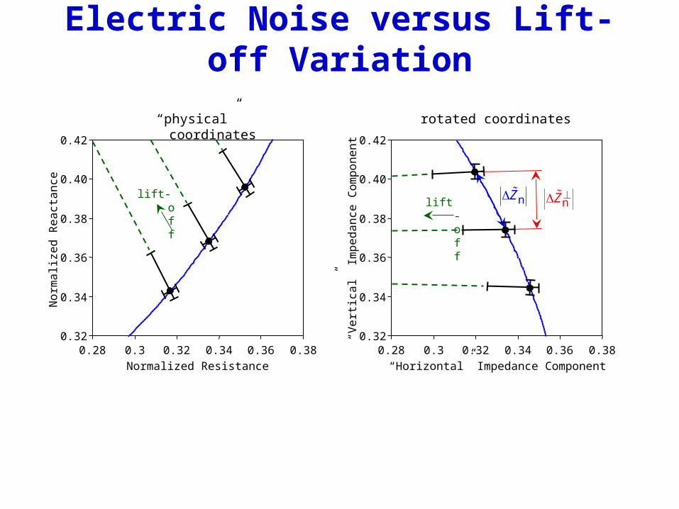
Electric Noise versus Lift-off Variation
0.32
0.34
0.36
0.38
0.40
0.42
0.28 0.3 0.32 0.34 0.36 0.38
“Horizontal” Impedance Component“V
erti
cal”
Im
peda
nce
Com
pone
nt0.32
0.34
0.36
0.38
0.40
0.42
0.28 0.3 0.32 0.34 0.36 0.38
Normalized Resistance
Nor
mal
ized
Rea
ctan
ce lift-offlift-off
“physical” coordinates rotated coordinates
nZ nZ

Conductivity Sensitivity, Gauge Factor
22 e e3 H, = 1 MHz, 10 , 1L f R R
nnorm
e e/
ZF
R R
n
abse e/
ZF
R R
0 (1 )R R F /
/
R RF
0
0.02
0.04
0.06
0.08
0.10
0.12
0.14
0 0.2 0.4 0.6 0.8 1
Frequency [MHz]
Gau
ge F
acto
r, F
absolute
normal0.32
0.34
0.36
0.38
0.40
0.42
0.28 0.3 0.32 0.34 0.36 0.38
Normalized Resistance
Nor
mal
ized
Rea
ctan
ce lift-off
nZ
nZ

Conductivity and Lift-off Trajectories
lift-off trajectories are not straightconductivity trajectories are not semi-circles
0
0.1
0.2
0.3
0.4
0.5
0.6
0.7
0.8
0.9
1
0 0.1 0.2 0.3 0.4 0.5
Normalized Resistance
Nor
mal
ized
Rea
ctan
ce
κ
lift-off
conductivity
eL
RA
( )
e ( )
LR
A
( , ) finite probe size
0
0.1
0.2
0.3
0.4
0.5
0.6
0.7
0.8
0.9
1
0 0.1 0.2 0.3 0.4 0.5
Normalized Resistance
Nor
mal
ized
Rea
ctan
ce
κlift-off
conductivity

2.4 Test Coil Impedance
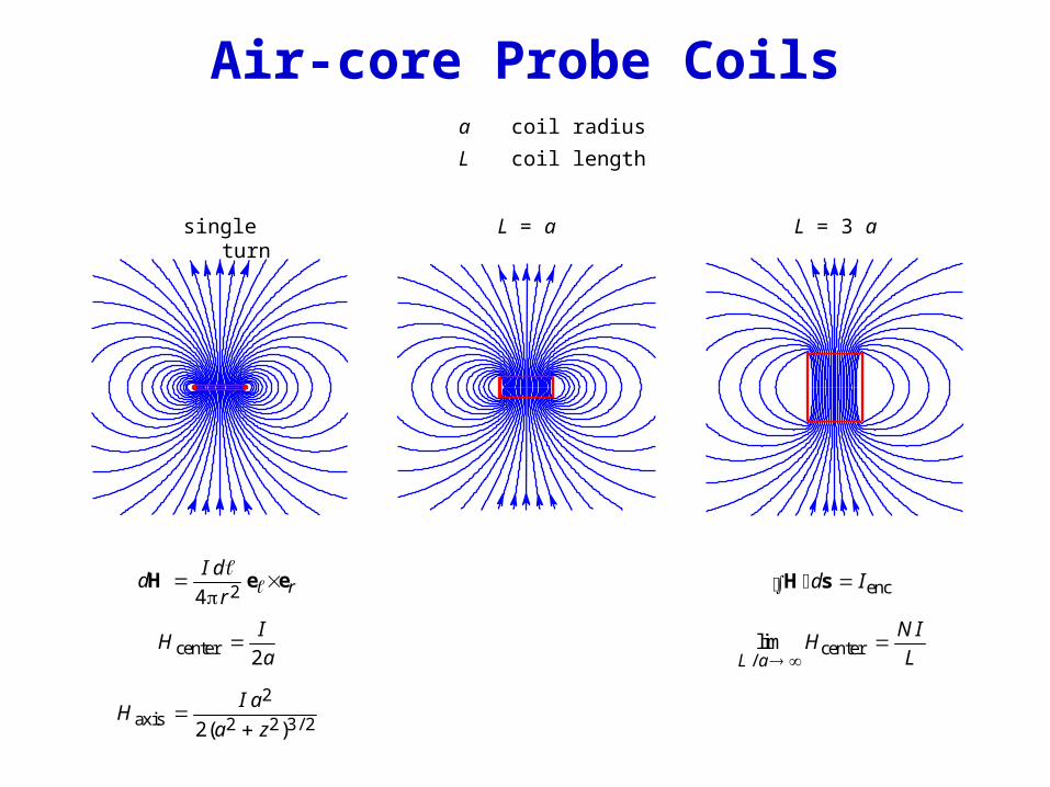
Air-core Probe Coils
single turn L = a L = 3 a
center 2
IH
a
24 rI d
dr
H e e
a coil radius
L coil length
encd IH s
center/lim
L a
N IH
L
2
axis 2 2 3/ 22( )
I aH
a z
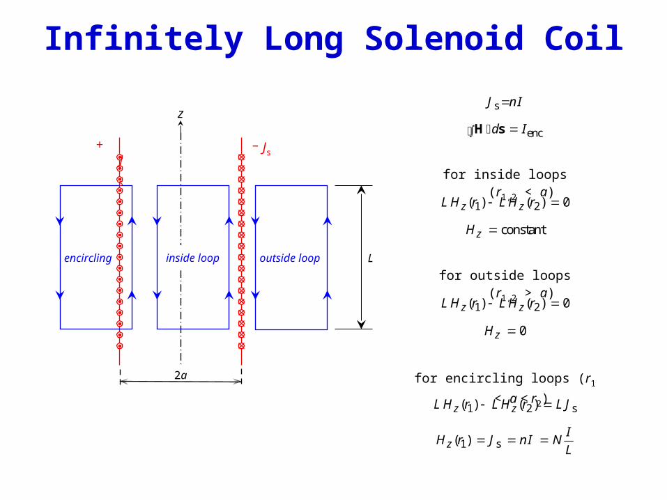
Infinitely Long Solenoid Coil
encd IH s
sJ n I
1 2( ) ( ) 0z zL H r L H r
for outside loops (r1,2 > a)
0zH
1 2( ) ( ) 0z zL H r L H r
for inside loops (r1,2 < a)
constantzH
1 2 s( ) ( )z zL H r L H r L J
1 s( )zI
H r J n I NL
for encircling loops (r1 < a < r2)
inside loop outside loopencircling
2a
L
+ Js_ Js
z

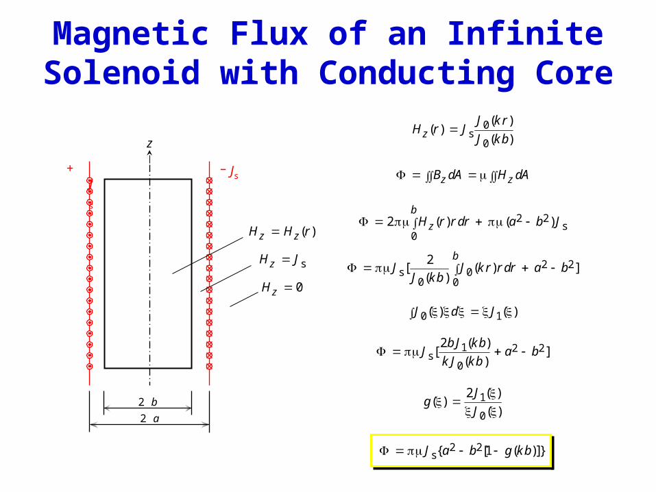
Magnetic Field of an Infinite Solenoid with Conducting Core
in the air gap (b < r < a) Hz = Js
in the core (0 < r < b) Hz = H1 J0(k r)
Jn nth-order Bessel function of the first kinds
10( )
JH
J k b
+ Js_ Js
2 a
2 b
z
0s
0
( )
( )zJ k r
H JJ k b
2 2( )k H 0 2k i 1 i
k
22
21
0zk Hr rr
2 2s
02 ( ) ( )
b
zH r r dr a b J
z zB dA H dA
Magnetic Flux of an Infinite Solenoid with Conducting Core
+ Js_ Js
2 a
2 b
z
0s
0
( )( )
( )zJ k r
H r JJ k b
( )z zH H r
szH J
0zH
2 2s 0
0 0
2[ ( ) ]
( )
bJ J k r r dr a b
J k b
0 1( ) ( )J d J
1 2 2s
0
2 ( )[ ]
( )
b J k bJ a b
k J k b
1
0
2 ( )( )
( )
Jg
J
2 2s [1 ( )]J a b g k b
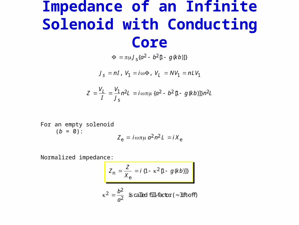
For an empty solenoid (b = 0):
Normalized impedance:
1 1 1, ,s LJ n I V i V NV n LV
1 2 2 2 2
s [1 ( )]LV V
Z n L i a b g k b n LI J
2 2e eZ i a n L i X
22
2is called fill-factor ( lift-off)
b
a
2n
e1 [1 ( )]
ZZ i g k b
X
2 2s [1 ( )]J a b g k b
Impedance of an Infinite Solenoid with Conducting Core

Resistance and Reactance of an Infinite Solenoid with Conducting Core
2n n n1 [1 ( )]Z i g k b R i X
0 Re ( ) 1g k b 0.4 Im ( ) 0g k b
2n Im ( )R g k b 2
n 1 [1 Re ( )]X g k b
n n1 RX m Re ( ) 1
Im ( )
g k bm
g k b
1 ik
(1 )
bk b i
22 2
bi
0.01 0.1 1 10 100 1000-0.4
-0.20.0
0.20.4
0.6
0.81.0
1.2
Normalized Radius, b/δ
g-fu
ncti
on
real part
imaginary part
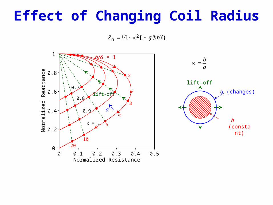
Effect of Changing Coil Radius
a (changes)
b (constant)
lift-off
b
a
Normalized Resistance
Nor
mal
ized
Rea
ctan
ce
0
0.2
0.4
0.6
0.8
1
0 0.1 0.2 0.3 0.4 0.5
b/δ = 1
3
5
10
20
2
κ = 1
0.9
0.8
0.7
a
lift-off
2n 1 [1 ( )]Z i g k b

Effect of Changing Core Radius
b (changing)
a (constant)
lift-off
2n 1 n 2 n1 R RX m m
b
a
n 1 21 0
1, where ( )
2a
a
Normalized Resistance
Nor
mal
ized
Rea
ctan
ce
0
0.2
0.4
0.6
0.8
1
0 0.1 0.2 0.3 0.4 0.5
100400
9
25
n = 4
κ = 1
0.9
0.8
0.7
b
lift-off
2n 1 [1 ( )]Z i g k b
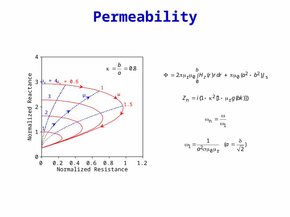
Permeability
Normalized Resistance
Nor
mal
ized
Rea
ctan
ce
0
1
2
3
4
0 0.2 0.4 0.6 0.8 1 1.2
ωn = 0.6
1.5
1
2
3
1
µr = 4
µ ω
0.8b
a
n1
2 2r 0 0 s
02 ( ) ( )
b
zH r r dr a b J
2n r1 [1 ( )]Z i g bk
1 20 r
1( )
2a
a
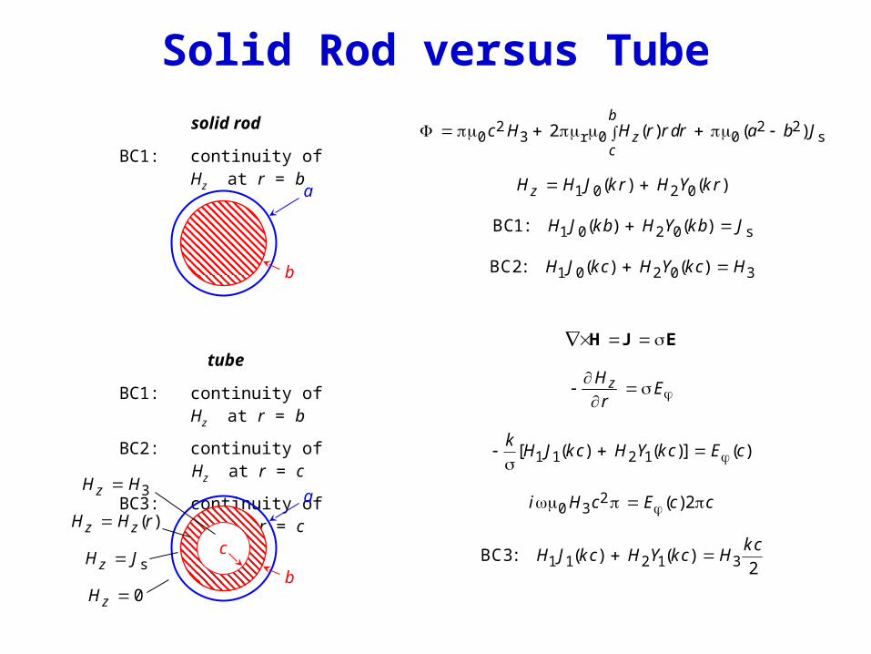
Solid Rod versus Tube
2 2 20 3 r 0 0 s2 ( ) ( )
b
zc
c H H r r dr a b J
1 0 2 0( ) ( )zH H J k r H Y k r
1 0 2 0 sBC1: ( ) ( )H J k b H Y k b J
1 0 2 0 3BC2: ( ) ( )H J k c H Y k c H
1 1 2 1 3BC3: ( ) ( )2
k cH J k c H Y k c H
b
a
1 1 2 1[ ( ) ( )] ( )k
H J k c H Y k c E c
H J E
zHE
r
20 3 ( )2i H c E c c
solid rod
BC1: continuity of Hz at r = b
tube
BC1: continuity of Hz at r = b
BC2: continuity of Hz at r = c
BC3: continuity of Eφ at r = c
b
a
c
( )z zH H r
szH J
0zH
3zH H

Solid Rod versus Tube
b
a
c
1,b c
a b
0
0.2
0.4
0.6
0.8
1
0 0.1 0.2 0.3 0.4 0.5 0.6Normalized Resistance
very thin
solid rod
tube
Nor
mal
ized
Rea
ctan
ce
thick tube
σ1
σ2
σ1
σ2

Wall Thickness
b
a
c
1,b c
a b
0
0.2
0.4
0.6
0.8
1
0 0.1 0.2 0.3 0.4 0.5 0.6
η = 0solid rod
b/ = 3
b/ = 2
Normalized Resistance
Nor
mal
ized
Rea
ctan
ce
b/ = 5
b/ = 10
b/ = 20 η 1thin tube
η = 0.2η = 0.4η = 0.6η = 0.8
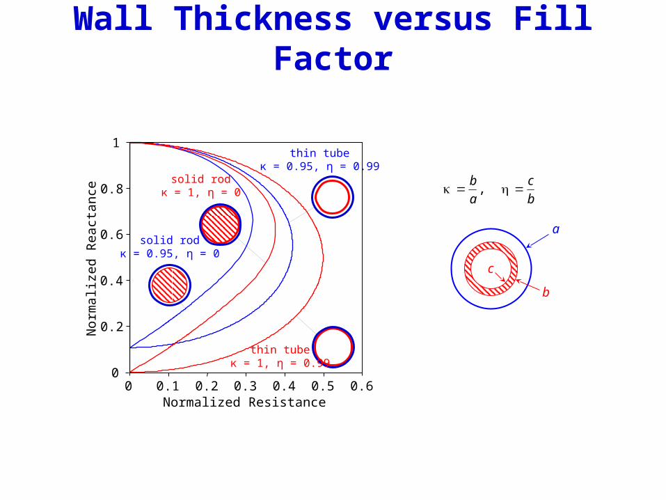
Wall Thickness versus Fill Factor
b
a
c
,b c
a b
0
0.2
0.4
0.6
0.8
1
0 0.1 0.2 0.3 0.4 0.5 0.6Normalized Resistance
Nor
mal
ized
Rea
ctan
ce
solid rodκ = 0.95, η = 0
solid rodκ = 1, η = 0
thin tubeκ = 1, η = 0.99
thin tubeκ = 0.95, η = 0.99

Clad Rod
b
a
c
2 2core core clad clad 0 s
02 ( ) 2 ( ) ( )
c b
cH r r dr H r r dr a b J
clad 1 0 clad 2 0 clad( ) ( )H H J k r H Y k r c r b
core 3 0 core( ) 0H H J k r r c
0
0.2
0.4
0.6
0.8
1
0 0.1 0.2 0.3 0.4 0.5 0.6Normalized Resistance
Nor
mal
ized
Rea
ctan
ce
copper claddingon brass coresolid
copper rod
solidbrass rodbrass cladding
on copper core
d
master curve forsolid rod
d
thin wall
lower fill factor
clad
core, ,
b c
a b
(1 )d b c b

2D Axisymmetric Models
b
a
c
2ao
2ai
t
h
ℓ
short solenoid (2D)
↓long solenoid (1D)
↓thin-wall long solenoid (≈0D)
↓ coupled coils (0D)
pancake coil (2D)
o
i
1( ) ( )a
aI x J x dx
2 20
2 2 60o i
( )( )
( )
i N IZ f d
h a a
r 1( ) 2
r 1( ) 2( 1) [ ]h hf h e e e
2 2 2 2r 01 k i
Dodd and Deeds. J. Appl. Phys. (1968)

Flat Pancake Coil (2D)
0
0.05
0.1
0.15
0.2
0.1 1 10 100
Frequency [MHz]
(Nor
mal
) G
auge
Fac
tor
4 mm
2 mm
1 mm
coil diameter
o iM 2
1
2
a aa f
a
a0 = 1 mm, ai = 0.5 mm, h = 0.05 mm, = 1.5 %IACS, = 0
0
0.2
0.4
0.6
0.8
1
0 0.05 0.1 0.15 0.2 0.25 0.3
Normalized Resistance
Nor
mal
ized
Rea
ctan
ce
0 mm
0.05 mm
0.1 mm
lift-off
frequency
fM
2.5 Field Distributions

Field Distributions
air-core pancake coil (ai = 0.5 mm, ao = 0.75 mm, h = 2 mm), in Ti-6Al-4V (σ = 1 %IACS)
10 Hz
10 kHz
1 MHz
10 MHz
1 mm
magnetic field
2 2r zH H H
electric field Eθ
(eddy current density)

Axial Penetration Depth air-core pancake coil (ai = 0.5 mm, ao = 0.75 mm, h = 2 mm) in Ti-6Al-4V
Axi
al P
enet
rati
on D
epth
, δ a
[m
m]
10-2
10-1
100
101
Frequency [MHz] 10-5 10-4 10-3 10-2 10-1 100 101 102
standard
actual1
f
ai
i o1
1/e point below the surface at ( )2
r a a a

1 22a a
Radial Spread air-core pancake coil (ai = 0.5 mm, ao = 0.75 mm, h = 2 mm) in Ti-6Al-4V
Rad
ial S
prea
d, a
s [m
m]
Frequency [MHz] 10-5 10-4 10-3 10-2 10-1 100 101 102
analytical
finite element
0.8
1.2
1.6
2.0
1.0
1.4
1.8
1/e point from the axis at the surface ( 0)z
2 o1.2a a

Radial Penetration Depth air-core pancake coil (ai = 0.5 mm, ao = 0.75 mm, h = 2 mm) in Ti-6Al-4V
Rad
ial P
enet
rati
on D
epth
, δr
[mm
]
10-2
10-1
100
101
Frequency [MHz] 10-5 10-4 10-3 10-2 10-1 100 101 102
standard
actual1
f
r s 2a a
2 o1.2a a
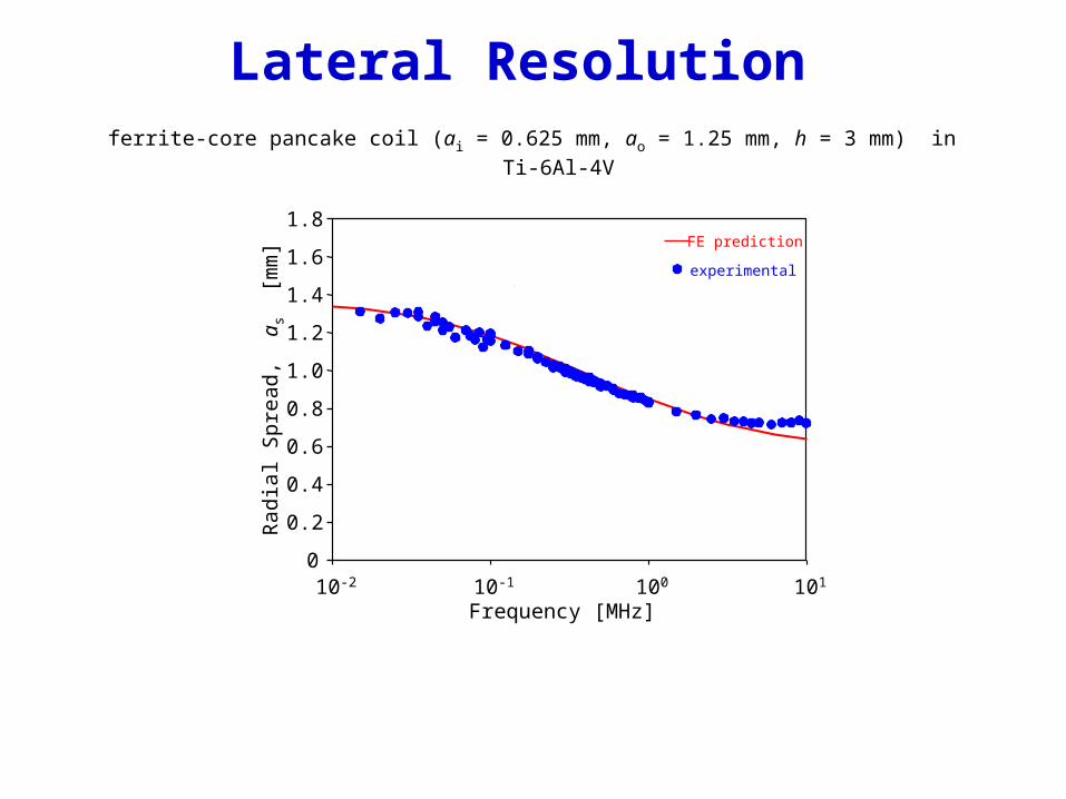
Lateral Resolution ferrite-core pancake coil (ai = 0.625 mm, ao = 1.25 mm, h = 3 mm) in Ti-6Al-4V
1.0
0
0.2
0.4
0.6
0.8
1.2
1.4
1.6
1.8
experimental
FE prediction
Rad
ial S
prea
d, a
s [m
m]
Frequency [MHz] 10-2 10-1 100 101