1D ﬁnite element for modelling of turbine blade vibration

Applied and Computational Mechanics 13 (2019) 107–124

1D finite element for modelling of turbine blade vibrationin the field of centrifugal forces

J. Dupala,∗, M. Zajıceka, V. Lukesa

aNTIS – New Technologies for the Information Society, Faculty of Applied Sciences, University of West Bohemia,Technicka 8, Pilsen, Czech Republic

Received 26 September 2018; accepted 18 December 2019

Abstract

The paper deals with the modelling of turbine blade vibrations by means of a novel 1D finite element that has only 16degrees of freedom. Assuming linear elastic behaviour of the blade material and considering small displacementsand strains, the derived blade finite element takes into account the effects of tension, torsion and bending inaccordance with the Bernoulli’s hypothesis. Additionally, the finite element interlinks bending and torsion, andrespects membrane forces acting on the blade. The derivation of matrices and vectors describing the blade finiteelement is provided in detail by using the Lagrange’s equations while the effect of membrane forces is includedvia the virtual work principle. For modelling purposes, the mathematical model of a turbine blade requires only theknowledge of cross-section contour points at several selected sections along the turbine blade axis. On the basis ofthese points, cross-section characteristics including the warping function are approximated along the blade axis bymeans of cubic splines. The advantage of this approach lies in the fact that all the blade cross-section parametersare identified before running numerical simulations. The warping function introduced in this paper and derived byvariational principle describes cross-section warping caused just by torsion of a prismatic rod.

For the verification of the proposed 1D finite element, an analysis of modal properties of the turbine bladeM6 L-1 manufactured by Doosan Skoda Power is performed. This is achieved by comparing the lowest naturalfrequencies and corresponding mode shapes computed by the 1D and 3D models for a standing blade. The resultsrevealed good agreement between both models despite the significant difference in their degrees of freedom. Theapplicability of the 1D finite element is further demonstrated by analyzing the dependence of natural frequencieson rotor speed.c© 2019 University of West Bohemia. All rights reserved.

Keywords: blade finite element, rotor speed, warping function, natural frequencies

1. Introduction

Many papers and books focused on problems concerning turbine blade dynamics and vibrationswere published in the past. At the beginning of research, entire blades were modelled asa 1D continuum and described by equations of motion including equilibrium conditions ofan infinitesimal element. The solution of derived partial differential equations describing motionof the blade was sought by approximate methods, because the use of computers was very limited.One of the earlier works published in the field of vibrations was written by Filipov [4]. Modellingof a blade packet by means of simple beams coupled with discrete massless springs was shownin paper [1], where each blade was modelled as a massless beam with mass concentrated at itsends. Here, the number of degrees of freedom (DOF) corresponded to a number of blades. Thisvery simplified model takes into account only the first mode shapes of individual blades.

∗Corresponding author. Tel.: +420 377 632 316, e-mail: [email protected]://doi.org/10.24132/acm.2019.463

107

https://doi.org/10.24132/acm.2019.463

J. Dupal et al. / Applied and Computational Mechanics 13 (2019) 107–124

Progress in the finite element (FE) method led to application of the aforementioned modellingapproach to turbine blade dynamics and related fields. Selected theoretical works dealt withinteraction of a bladed wheel with steam aerodynamic forces [7] or with mutual interactionbetween individual blades caused by frictional forces [9]. The last mentioned work dealt with avery interesting approach that uses cyclic symmetry for the reduction of the DOF. This approachallows to respect even other nonlinear forces between individual blades, while the solution isperformed in frequency domain. The recent papers [8] and [6] presented non-linear dynamicanalysis of a friction member between blades. However, the used models were simple, e.g., themodel mentioned in [8] is only a 2-DOF system.

The majority of current works considers models that use the FE analysis by means of 3Delements. Not only due to high computational costs, the complex models usually include onlyseveral blades, bladed packets or an entire bladed disc. To simulate the behaviour of a wholeturbo-machine with minimal costs, another approach is necessary. For this purpose, the presentpaper introduces a novel 1D rotating FE model that despite its relatively low number of DOF isable to well approximate the behaviour of a 3D blade.The description of the finite element, whichwill be derived in the following sections, includes all beam properties and the pre-processor forwarping function calculation and takes into account the variability of blade cross-section alongthe blade axis. Additionally, the following kinematical considerations are applied:

• The cross-section projection into the plane perpendicular to the blade axis remains un-changed.

• The kinetic and potential energies of the blade finite element respect warping of thecross-section.

• The material of the blade finite element satisfies the Hooke’s law.• The material of the blade finite element is assumed to be homogeneous and isotropic.• Bending deflections of the blade are considered to be small and corresponding rotations

can be expressed as their derivatives.• The cross-section characteristics are approximated by cubic polynomials along the blade

axis.• The blade model respects membrane forces.

2. Mathematical description of the 1D finite element

In this section, the mathematical background of the proposed 1D blade finite element is given.This is achieved firstly by introducing the kinematics of displacements, expressing the kineticand deformation potential energies of the finite element and outlining the calculation of the cross-section warping function. Consequently, the matrices and vectors describing the finite elementare derived by applying the Lagrange’s equations and by assuming the effect of membrane force.Lastly, the equations of motion of one finite element as well as those of the entire blade areassemblied.

2.1. Kinematics of displacements

For a better understanding of the following sections, let us introduce a coordinate system ξ, η, ζ ,where ξ is an arbitrarily chosen axis in the direction of the longest blade dimension (the bladeaxis mentioned above). The axis η is parallel with the vector of angular speed ω and the thirdaxis ζ is completed in such a way to get a right-handed coordinate system shown in Fig. 1. Notethat this system ξ, η, ζ defines the rotating coordinate system of the rotor.

108


Fig. 1. Coordinate system of the blade and shear centre displacements

The coordinate system ξ, η, ζ rotates at the constant angular speed ω about the axis η whichis identical to the axis of the turbine rotor. The intersection of ξ axis with the blade cross-sectionis marked as point P . Let us consider the beginning of the finite element in the distance r fromthe axis of rotation. Then, the motion of an arbitrary point of the cross-section at the coordinate ξcan be decomposed into the primary sliding motion of the reference point S∗ from the initialstate point S (displacements of the cross-section shear centre uS, vS, wS) and the secondaryspherical motion of the rigid cross-section caused by bending (ψ, ϑ) and torsion (ϕ) and thetertiary motion in the x-direction caused by warping. Consequently, the radius-vector of theshear centre in coordinate system ξ, η, ζ can be expressed in the form

rS =

⎡⎣ uS

vSwS

⎤⎦ =

⎡⎣ r + ξ + u0 − (ηS − ηC)ψ + (ζS − ζC)ϑ

ηS + v0ζS + w0

⎤⎦ , (1)

where u0 corresponds to the displacement of all cross-section points in the ξ direction causedby the tension and ηS, ζS and ηC, ζC denote the coordinates of the shear centre and the cross-section centroid, respectively. The symbols w0 and v0 denote the displacements in the ζ and ηdirections caused by the bending in planes ξζ and ξη, respectively. Due to the assumption ofsmall displacements, the angles associated with the bending can be written as

ϑ = −∂w0∂ξ= −w′

0, ψ =∂v0∂ξ= v′

0. (2)

Taking the shear centre as a reference point, we can express the radius vector r of an arbitrarypoint of the blade cross-section in the coordinate system ξ, η, ζ in the following form

r = rS +Tr, (3)

109


where r is the radius vector of the arbitrary point in the coordinate systems x, y, z and T is thetransformation matrix from the x, y, z coordinate system to the ξ, η, ζ coordinate system

T =

⎡⎣ cosψ cosϑ, sinϕ sinϑ − cosϕ cosϑ sinψ, sin ϑ cosϕ+ cosϑ sinϕ sinψ

sinψ, cosψ cosϕ, − cosψ sinϕ− cosψ sin ϑ, cosϑ sinϕ+ sinϑ cosϕ sinψ, cosϑ cosϕ − sinϑ sinϕ sinψ

⎤⎦ . (4)

The radius vector r has the form

r =

⎡⎣ ϕ′g

y − ySz − zS

⎤⎦ , (5)

which means that the overall warping corresponds to a product of the warping function g and therelative twist ϕ′. For practical reasons, we express the velocity vector in the rotating coordinatesystem ξ, η, ζ as

r =drdt

∣∣∣∣ξηζ

+ω × r, (6)

where the angular speed vector ω = [0 ω 0]T corresponds to the rotation of the coordinatesystem ξ, η, ζ in relation to the stationary coordinate system.

2.2. Kinetic and deformation potential energies of one finite element

The kinetic energy in the form

EeK =

12ρ

∫ l

0

∫∫A

rT rdA dξ, (7)

where ρ is the density, can be derived by substituting (3), (4), (5) into (6). Due to the complexityof the resulting relation, it is not presented in this paper.

For the derivation of the deformation potential energy, the Bernoulli’s beam hypothesis istaken into consideration. According to this hypothesis, the deformation tensor consists only ofthe following non-zero components

εξ =∂u

∂ξ= u′

0 − (η − ηC)ψ′ + (ζ − ζC)ϑ

′ + ϕ′′g + ϕ′g′,

γξη =∂u

∂η+

∂v

∂ξ=

(∂g

∂η− ζ + ζS

)ϕ′, (8)

γξζ =∂u

∂ζ+

∂w

∂ξ=

(∂g

∂ζ+ η − ηS

)ϕ′,

where u is the displacement of the arbitrary point of the cross-section in the ξ direction andg′ denotes partial derivative of the warping function with respect to the coordinate ξ. By assumingthat the warping function varies slowly along the coordinate ξ, we can neglect the last term of(8)1. The Hooke’s law for the Bernoulli’s beam theory takes the form

σ = Eε, (9)

where σ = [σξ τξζ τξη]T is the stress vector, ε = [εξ γξζ γξη]T is the deformation vectorand E = diag(E G G) is a diagonal matrix, where E is the Young’s modulus and G is the

110


shear modulus. Then, the relation for the deformation potential energy of one finite element canbe written in the following form

EePd =

12

∫ l

0

∫∫A

σTεdA dξ =12

∫ l

0

∫∫A

(Eε2ξ +Gγ2ξη +Gγ2ξζ) dA dξ, (10)

or after substitution

EePd =

12

∫ l

0{E[A(u′

0)2 + Iζ(v

′′0)2 + Iη(w

′′0)2 + Iϕ(ϕ

′′)2 +

+2Dηζv′′0w

′′0 − 2Dηϕv′′

0ϕ′′ − 2Dζϕw′′

0ϕ′′] +GIK(ϕ

′)2} dξ, (11)

where

IK =∫∫

A

[(∂g

∂ζ+ η − ηS

)2+

(∂g

∂η− ζ + ζS

)2]dA (12)

is the so called torsion constant and

Iϕ =∫∫

A

g2 dA, Dϕη =∫∫

A

gη dA,

Dϕζ =∫∫

A

gζ dA, Dηζ =∫∫

A

(η − ηC)(ζ − ζC) dA. (13)

The bar over subscripts in Dηζ denotes a quantity in the coordinate system with the origin in thecross-section centroid.

2.3. Calculation of the warping function

In this paper, the cross-section warping caused only by blade torsion is taken into account. Thecalculation of the warping function is performed supposing clear and free torsion of a prismaticrod.

Let us assume that the cross-section rotates about the yet unknown point called the shearcentre. Taking into consideration clear torsion, the first three terms at the right hand side of(8)1 are equal to zero because these terms correspond to the deformations caused by tensionand bending. The fourth term is zero because the torsion angle ϕ is linearly dependent on thecoordinate ξ, and thus, ϕ′′ = 0. The last term in (8)1 is also equal to zero because the warpingfunction g is constant in the case of clear torsion of the prismatic rod. Then, for the twistedprismatic rod, the potential energy of an infinitesimal element of length dξ can be written in theform

1dξ

EPd =12

∫∫A

G(γ2ξη + γ2ξζ) dA, (14)

where γξη and γξζ express shear strains given by relations (8)2 and (8)3. The substitution of (8)into (14) and the addition of external effect yield

1dξ

EP =Gϕ′2

2

∫∫A

[(∂g

∂η− ζ + ζS

)2+

(∂g

∂ζ+ η − ηS

)2]dA − ϕ′Mξ, (15)

where Mξ is the external torsional moment. Relation (15) contains the total potential energy ofdeformation and external forces EP . To obtain a unique solution of (15), it is necessary to addthe following three conditions:∫∫

A

g dA = 0,∫∫

A

gη dA = 0,∫∫

A

gζ dA = 0, (16)

111


ensuring zero normal force and two bending moments related to axes η and ζ . From the secondand third conditions in (16), it is possible to get Dϕη = 0, Dϕζ = 0.

The solution of the warping function will correspond to a minimum of the followingfunctional

J =G(ϕ′)2

2

∫∫A

[(∂g

∂ζ+ η − ηS

)2+

(∂g

∂η− ζ + ζS

)2]dA − ϕ′Mξ +

+λ∗1

∫∫A

g dA+ λ∗2

∫∫A

ηg dA + λ∗3

∫∫A

ζg dA, (17)

where λ∗1, λ∗

2, λ∗3 are the Lagrange’s multipliers. In (17), there are seven independent quantities

ϕ′, g, ηS, ζS, λ∗1, λ

∗2, λ

∗3 because the shear centre coordinates are still unknown. Then, a functional

variation takes the form

δJ = Gϕ′∫∫

A

[(∂g

∂ζ+ η − ηS

)2+

(∂g

∂η− ζ + ζS

)2]dAδϕ′ +

+G(ϕ′)2∫∫

A

[(∂g

∂ζ+ η − ηS

)∂

∂ζ(δg) +

(∂g

∂η− ζ + ζS

)∂

∂η(δg)

]dA +

+G(ϕ′)2∫∫

A

[−

(∂g

∂ζ+ η − ηS

)δηS +

(∂g

∂η− ζ + ζS

)δζS

]dA −

−Mξδϕ′ + δλ∗

1

∫∫A

g dA + λ∗1

∫∫A

δg dA + δλ∗2

∫∫A

ηg dA+ λ∗2

∫∫A

ηδg dA+

+δλ∗3

∫∫A

ζg dA + λ∗3

∫∫A

ζδg dA = 0. (18)

Because the individual variations are independent of each other, the terms contained in thesevariations must be equal to zero, resulting in a system of seven equations

(GIKϕ′ − Mξ)δϕ′ = 0, (19)

G(ϕ′)2∫∫

A

[(∂g

∂ζ+ η − ηS

)∂

∂ζ(δg) +

(∂g

∂η− ζ + ζS

)∂

∂η(δg)

]dA+

+λ∗1

∫∫A

δg dA+ λ∗2

∫∫A

ηδg dA + λ∗3

∫∫A

ζδg dA = 0, (20)

−G(ϕ′)2∫∫

A

(∂g

∂ζ+ η − ηS

)dAδηS = 0, (21)

G(ϕ′)2∫∫

A

(∂g

∂η− ζ + ζS

)dAδζS = 0, (22)

δλ∗1

∫∫A

g dA = 0, (23)

δλ∗2

∫∫A

ηg dA = 0, (24)

δλ∗3

∫∫A

ζg dA = 0. (25)

Equation (19) is a torque equilibrium condition independent of the other ones. The remainingsix equations (20)–(25) are used for the calculation of unknown quantities g, ηS, ζS, λ∗

1, λ∗2, λ∗

3.

112


The FE discretization of (20)–(25) leads to a system of (n+5) linear algebraic equations, wheren corresponds to the number of discretization points of the cross-section area as well as to thenumber of function values of the warping function. Then, the vector of unknowns can take thefollowing form

x = [gT ηS ζS λ∗1 λ∗

2 λ∗3]T ∈ Rn+5,1, (26)

where g ∈ Rn,1 is the function value vector of the warping function at the discretization points.

2.4. Approximations of displacements and of cross-section characteristics

The displacements in the ξ, η, ζ directions and the corresponding torsion and bending angles ϕ,ψ, ϑ can be approximated as

u0(ξ)=Φ(ξ)S−1q3, v0(ξ)=Φ(ξ)S−1q1, w0(ξ)=Φ(ξ)S−1Pq2,

ϕ(ξ)=Φ(ξ)S−1q4, ψ(ξ)= v′0(ξ) = Φ

′(ξ)S−1q1, ϑ(ξ)=−w′0(ξ) = −Φ′(ξ)S−1Pq2,

(27)

where

q1 =

⎡⎢⎢⎣

v0(0)ψ(0)v0(l)ψ(l)

⎤⎥⎥⎦ , q2 =

⎡⎢⎢⎣

w0(0)ϑ(0)w0(l)ϑ(l)

⎤⎥⎥⎦ , q3 =

⎡⎢⎢⎣

u0(0)u′0(0)

u0(l)u′0(l)

⎤⎥⎥⎦ , q4 =

⎡⎢⎢⎣

ϕ(0)ϕ′(0)ϕ(l)ϕ′(l)

⎤⎥⎥⎦

and

Φ(ξ) = [1 ξ ξ2 ξ3], S =

⎡⎢⎢⎣1 0 0 00 1 0 01 l l2 l3

0 1 2l 3l2

⎤⎥⎥⎦ , P = diag(1 −1 1 −1).

Prime derivative for tensile deformations was used due to the variability of the blade profile andbecause it is appropriate to use higher order polynomials instead of linear ones. Because theuse of quadratic polynomials without derivatives would require an extra mid-site node for eachfinite element, the present study applies cubic polynomials and considers derivatives at the endsof the elements.

The same degree of approximation (cubic polynomials) are used for the approximation ofcross-section characteristics along the coordinate ξ, leading to the following relations:

A(ξ)=3∑

i=0

ai1ξi = Φ(ξ)a1, Iζ(ξ)=

3∑i=0

ai2ξi = Φ(ξ)a2,

Iη(ξ)=3∑

i=0

ai3ξi = Φ(ξ)a3, Iϕ(ξ)=

3∑i=0

ai4ξi = Φ(ξ)a4,

E1(ξ)=3∑

i=0

ai5ξi = Φ(ξ)a5, E2(ξ)=

3∑i=0

ai6ξi = Φ(ξ)a6,

I∗ζ (ξ)=

3∑i=0

ai7ξi = Φ(ξ)a7, I∗

η (ξ)=3∑

i=0

ai8ξi = Φ(ξ)a8,

113


S∗ζ (ξ)=

3∑i=0

ai9ξi = Φ(ξ)a9, Dηζ(ξ)=

3∑i=0

ai10ξi = Φ(ξ)a10,

Sη(ξ)=3∑

i=0

ai11ξi = Φ(ξ)a11, Dη∗ζ(ξ)=

3∑i=0


S∗η(ξ)=

3∑i=0

ai13ξi = Φ(ξ)a13, IK(ξ)=

3∑i=0


E3(ξ)=3∑

i=0


(28)

where

E1(ξ) = A(ξ)ζC(ξ)[ηS(ξ)− ηC(ξ)],

E2(ξ) = A(ξ)ζC(ξ)[ζS(ξ)− ζC(ξ)],

E3(ξ) = A(ξ)[η2S(ξ)− 2ηS(ξ)ηC(ξ) + ζS(ξ)ζC(ξ)] + Iζ(ξ)− Iη(ξ).

2.5. Matrices and vectors describing the blade finite element

2.5.1. Application of the Lagrange’s equations

For the assembling of matrices and vectors describing the blade finite element, the Lagrange’sequations are used in the first place. The application of the left hand side of the Lagrange’sequations to the kinetic and deformation potential energies from Section 2.2 and the use of theapproximations of displacements and of cross-section characteristics given in Section 2.4 yield

ddt

(∂Ee

K

∂ ˙qe

)− ∂Ee

K

∂qe

+∂Ee

Pd

∂qe

= Me ¨qe(t) + ωGe ˙qe(t) + (Ke + KeD)qe(t)− fDe. (29)

In (30), the vector of generalized displacements has the following form

qe = [qT1 qT2 qT3 qT4 ]T. (30)

The symbol Me represents the FE mass matrix, ωGe is the FE matrix of gyroscopic effects, Ke

is the FE stiffness matrix, KeD is the FE circulation matrix and fDe is the FE vector of centrifugal

forces. For better clarity, the specific forms of these matrices and the vector of centrifugalforces can be found in the Appendix of this paper. Note that compared to the cross-sectioncharacteristics listed in (28), which depend on the coordinate ξ, the material parameters ρ, Eand G appearing in the aforementioned matrices and the vector are assumed to be constantwithin one finite element.

2.5.2. Membrane generalized force vector

In this section, the effect of the membrane force is included into the mathematical model of theblade finite element. For this purpose, it is necessary to express the action of the force S(ξ) inthe transverse directions η and ζ , see Fig. 2.

In accordance with Fig. 2, the force resultant in the direction η has the form

dV = S sinψ +∂(S sinψ)

∂ξdξ − S sinψ. (31)

114


Fig. 2. Front and plan views of the membrane force acting in the longitudinal direction

Fig. 3. Axial force acting on the blade

By assuming the angle ψ to be small and taking (2)2 into consideration, (31) can be rewritten as

dV =

(∂S

∂ξ

∂v0∂ξ+ S

∂2v0∂ξ2

)dξ = (S ′v′

0 + Sv′′0) dξ. (32)

Analogously, the force resultant in the direction ζ can be derived, i.e., by considering the angle ϑto be small and respecting (2)1,

dW =

(∂S

∂ξ

∂w0∂ξ+ S

∂2w0∂ξ2

)dξ = (S ′w′

0 + Sw′′0) dξ. (33)

To be able to apply relations (32) and (33), the determination of the axial force S(ξ) has to beperformed. As apparent from Fig. 3, the origin of the coordinate ξ for the blade finite elementlies in the distance r from the axis of rotation. The axial force So acting on the finite elementfrom the rest of the blade can be expressed in the form So = Δmeω2, whereΔm is the mass ofthe remaining part of the blade in the direction ξ and e is its centroid eccentricity. Then, using

115


the approximation of A(s) from (28), the axial force can be written as

S(ξ) = Δmeω2 + ρω2∫ l−ξ

0A(s)(r + ξ + s) ds =

= Δmeω2 + ρω2∫ l−ξ

0

3∑i=0

ai1si(r + ξ + s) ds. (34)

The integration of (34) results in

S(ξ) = Δmeω2 + ρω23∑

i=0

ai1

{(l − ξ)i+1

i+ 1(r + ξ) +

(l − ξ)i+2

i+ 2

}(35)

and its corresponding derivative with respect to ξ

S ′(ξ) = ρω23∑

i=0

ai1

{(l − ξ)i+1

i+ 1− (l − ξ)i(r + ξ)− (l − ξ)i+1

}. (36)

By substituting (35) and (36) into (32) and (33), the membrane forces acting on the infinitesimalelement in the directions η and ζ can be obtained

dV =

{v′′

[Δmeω2 + ρω2

3∑i=0

ai1

⟨(l − ξ)i+1

i+ 1(r + ξ) +

(l − ξ)i+2

i+ 2

⟩]+

+ v′ρω23∑

i=0

ai1

[(l − ξ)i+1

i+ 1− (l − ξ)i(r + ξ)− (l − ξ)i+1

]}dξ, (37)

dW =

{w′′

[Δmeω2 + ρω2

3∑i=0

ai1

⟨(l − ξ)i+1

i+ 1(r + ξ) +

(l − ξ)i+2

i+ 2

⟩]+

+ w′ρω23∑

i=0

ai1

[(l − ξ)i+1

i+ 1− (l − ξ)i(r + ξ)− (l − ξ)i+1

]}dξ. (38)

In (37) and (38), the terms in curly brackets represent loads (force per unit length) caused bymembrane forces. Their virtual work over the whole finite element can be expressed by relations

δWv =∫ l

0δv(ξ)

{v′′(ξ)

[Δmeω2 + ρω2

3∑i=0

ai1

⟨(l − ξ)i+1

i+ 1(r + ξ) +

(l − ξ)i+2

i+ 2

⟩]+

+ v′(ξ)ρω23∑

i=0

ai1

[(l − ξ)i+1

i+ 1− (l − ξ)i(r + ξ)− (l − ξ)i+1

]}dξ, (39)

δWw =∫ l

0δw(ξ)

{w′′(ξ)

[Δmeω2 + ρω2

3∑i=0

ai1

⟨(l − ξ)i+1

i+ 1(r + ξ) +

(l − ξ)i+2

i+ 2

⟩]+

+ w′(ξ)ρω23∑

i=0

ai1

[(l − ξ)i+1

i+ 1− (l − ξ)i(r + ξ)− (l − ξ)i+1

]}dξ. (40)

116


The substitution of the approximations (27) into (39) and (40) and their integration over ξ yield

fM1 = ρω2S−T3∑

i=0

ai1

[1

i+ 1Ji+101 − (r + l)Ji

01

]S−1q1 +Δmeω2S−TJ002S

−1q1 +

+ρω2S−T3∑

i=0

ai1

[r + l

i+ 1Ji+102 +

(1

i+ 2− 1

i+ 1

)Ji+202

]S−1q1, (41)

fM2 = ρω2PS−T3∑

i=0

ai1

[1

i+ 1Ji+101 − (r + l)Ji

01

]S−1Pq2 +Δmeω2PS−TJ002S

−1Pq2 +

+ρω2PS−T3∑

i=0

ai1

[r + l

i+ 1Ji+102 +

(1

i+ 2− 1

i+ 1

)Ji+202

]S−1Pq2, (42)

fM3 = fM4 = 0. (43)

Note that for the sake of clarity, special integrating matrices

Jkij =

∫ l

0κkΦTi (κ)Φj(κ) dκ, i, j = 0, 1, 2, Φ0(κ) = Φ(κ), (44)

were introduced in (41) and (42) by taking the following substitutions into consideration

ξ → l − κ, dξ → −dκ, Φ(ξ)→ Φ(κ) = [1, l − κ, (l − κ)2, (l − κ)3],

Φ′(ξ)→ Φ1(κ) = [0, 1, 2(l − κ), 3(l − κ)2], Φ′′(ξ)→ Φ2(κ) = [0, 0, 2, 6(l − κ)].

Finally, the entire vector of membrane forces acting on a blade finite element can be written as

fMe =

⎡⎢⎢⎣fM1fM200

⎤⎥⎥⎦ =

⎡⎢⎢⎣KM11 0 0 00 KM

22 0 00 0 0 00 0 0 0

⎤⎥⎥⎦

︸︷︷︸Ke

M

⎡⎢⎢⎣q1q2q3q4

⎤⎥⎥⎦ = ω2

⎡⎢⎢⎣MM11 0 0 00 MM

22 0 00 0 0 00 0 0 0

⎤⎥⎥⎦

︸︷︷︸Me

M

⎡⎢⎢⎣q1q2q3q4

⎤⎥⎥⎦ , (45)

whereKe

M = ω2MeM ∈ R16,16

and the individual submatrices have the form

KM11 = ω2MM

11 = ρω2S−T3∑

i=0

ai1

[1

i+ 1Ji+101 − (r + l)Ji

01

]S−1 +Δmeω2S−TJ002S

−1 +

+ρω2S−T3∑

i=0

ai1

[r + l

i+ 1Ji+102 +

(1

i+ 2− 1

i+ 1

)Ji+202

]S−1 (46)

and

KM22 = ω2MM

22 = ρω2PS−T3∑

i=0

ai1

[1

i+ 1Ji+101 − (r + l)Ji

01

]S−1P+

+Δmeω2PS−TJ002S−1P+

+ρω2PS−T3∑

i=0

ai1

[r + l

i+ 1Ji+102

(1

i+ 2− 1

i+ 1

)Ji+202

]S−1P. (47)

117


2.6. Total equations of motion

With reference to Section 2.5, the total equations of motion for a blade finite element can beexpressed as

Me ¨qe(t) + ωGe ˙qe(t) + (Ke + KeD)qe(t) = fZe(t) + fDe + fMe, (48)

where fZe(t) is the vector of remaining external forces. With respect to (A5) and (45), thematrix Ke

D and the vector fMe in (48) can be modified leading to the equations of motion in thefollowing form

Me ¨qe(t) + ωGe ˙qe(t) + (Ke − ω2MeD − ω2Me

M)qe(t) = fZe(t) + fDe. (49)

From the practical point of view, the sequence of general displacements in qe (and forces)can be rearranged in such a way that the first 8 vector components correspond to the first nodeof finite element and the remaining 8 vector components to the second one. This rearrangementcan be performed with the help of a permutation matrix J, i.e., all matrices and vectors in (49)are transformed as Me = JTMeJ and qe = JTqe and fZe(t) = JTfZe(t) etc. Then, the totalequations of motion for the blade finite element have the final form

Meqe(t) + ωGeqe(t) + (Ke − ω2MeD − ω2Me

M)qe(t) = fZe(t) + fDe. (50)

To mathematically describe the motion of the entire blade, it is necessary to assembly thetotal matrices and vectors in a way that is standard in the FE analysis. Then, the equations ofmotion of the blade can be obtained in the following form, similar to (50),

Mq(t) + ωGq(t) + (K− ω2MD − ω2MM )q(t) = fZ(t) + fD. (51)

These equations describe a transient vibration of the blade.

3. Verification of the proposed blade finite element on the basis of modal properties

At the beginning, it should be pointed out that the calculation of the warping function outlinedin Section 2.3 was performed supposing clear and free torsion of a prismatic rod. However,the blade can be generally of variable cross-section and be exposed to constrained torsion.Nevertheless, for the derived blade finite element, we consider simplifying assumptions thatthe warping function is identical for free and constrained torsion as well as for prismatic andnon-prismatic rods. It means that this function depends only on the cross-section shape. To beable to use the blade finite elements for modelling purposes, it is necessary to identify bladeparameters a priori to running any numerical simulation. Firstly, for each known section (alwaysperpendicular to the blade axis), the cross-section characteristics, the coordinates of the centerof gravity and the shear centre and the warping function have to calculated. Consequently,these parameters are approximated by means of cubic polynomials along the blade axis andpolynomial coefficients aij in (28) are determined for each blade finite element. Finally, it ispossible to assembly the corresponding matrices and vectors introduced in Section 2 and listedin Appendix.

The verification of the proposed 1D blade finite element is carried out on the model of theturbine blade M6 L-1 manufactured by Doosan Skoda Power. In this case, the geometry of thisblade is given by individual cross-section contour points obtained at 10 different sections alongthe turbine blade axis. Considering the zero angular speed (ω = 0), the modal behaviour of the

118


turbine blade is analyzed by means of 1D and 3D models, particularly of interest is the behaviourcorresponding to the lowest eigenfrequencies. For the 1D model based on the proposed finiteelement, all required input parameters are calculated as described in the previous paragraph. Inthe case of the 3D model, the geometry of the turbine blade is reconstructed using cubic splinesand the resulting volume is discretized with tetrahedral finite elements. The modal analysis,which includes the calculation of natural frequencies Ωi, i = 1, 2, . . . , n (n ∼ blade DOF), isbased on the following equations

(K− Ω2M)v = 0, (52)

where v is the eigenvector. The boundary conditions prescribed in both 1D and 3D modelscorrespond to a clamped low end and to a free upper end of the turbine blade. Although theseboundary conditions do not faithfully simulate the actual blade attachment, they are sufficientto verify suitability of the proposed 1D finite element.

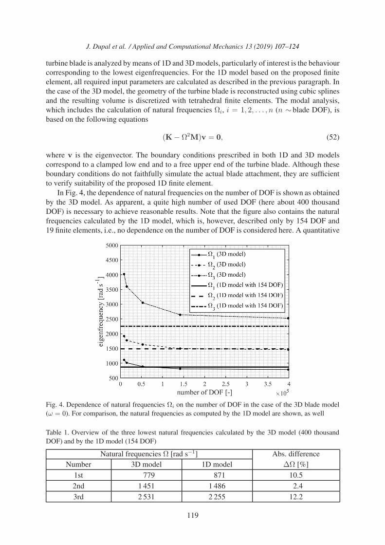
In Fig. 4, the dependence of natural frequencies on the number of DOF is shown as obtainedby the 3D model. As apparent, a quite high number of used DOF (here about 400 thousandDOF) is necessary to achieve reasonable results. Note that the figure also contains the naturalfrequencies calculated by the 1D model, which is, however, described only by 154 DOF and19 finite elements, i.e., no dependence on the number of DOF is considered here. A quantitative

Fig. 4. Dependence of natural frequencies Ωi on the number of DOF in the case of the 3D blade model(ω = 0). For comparison, the natural frequencies as computed by the 1D model are shown, as well

Table 1. Overview of the three lowest natural frequencies calculated by the 3D model (400 thousandDOF) and by the 1D model (154 DOF)

Natural frequencies Ω [rad s−1] Abs. differenceNumber 3D model 1D model ΔΩ [%]

1st 779 871 10.52nd 1 451 1 486 2.43rd 2 531 2 255 12.2

119


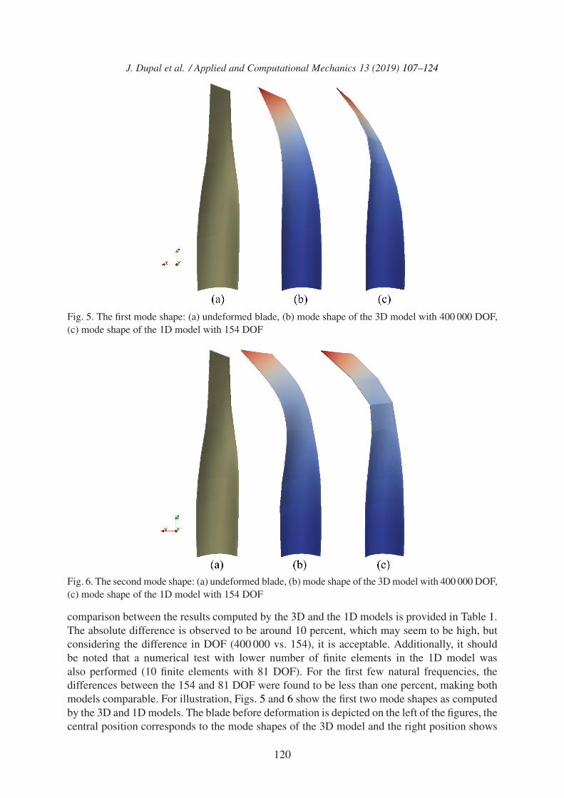
Fig. 5. The first mode shape: (a) undeformed blade, (b) mode shape of the 3D model with 400 000 DOF,(c) mode shape of the 1D model with 154 DOF

Fig. 6. The second mode shape: (a) undeformed blade, (b) mode shape of the 3D model with 400 000 DOF,(c) mode shape of the 1D model with 154 DOF

comparison between the results computed by the 3D and the 1D models is provided in Table 1.The absolute difference is observed to be around 10 percent, which may seem to be high, butconsidering the difference in DOF (400 000 vs. 154), it is acceptable. Additionally, it shouldbe noted that a numerical test with lower number of finite elements in the 1D model wasalso performed (10 finite elements with 81 DOF). For the first few natural frequencies, thedifferences between the 154 and 81 DOF were found to be less than one percent, making bothmodels comparable. For illustration, Figs. 5 and 6 show the first two mode shapes as computedby the 3D and 1D models. The blade before deformation is depicted on the left of the figures, thecentral position corresponds to the mode shapes of the 3D model and the right position shows

120


the mode shapes obtained by applying the presented methodology. In both cases, these figuresindicate a good agreement between the mode shapes from both computational blade models.

In the remainder of this section, the behaviour of the blade in a rotating coordinate system(ω �= 0) is studied. Because of the complex implementation of the 3D model (commercialsoftware usually do not offer the possibility to include effects of the rotating system), onlythe blade model described by the 1D finite elements is assumed. Then, the correspondingmathematical model has the form given by (51) with natural frequencies dependent on theangular speed ω. Compared to the previous paragraphs, the calculation of the frequenciescannot be performed according to (52), but the system of n second order differential equations(51) has to be converted to a system of 2n first order differential equations by using the followingtrivial identity

Mq(t)−Mq(t) = 0.Next, let us consider only the eigenvalue problem which involves the solution of the extendedsystem of equations

[P(ω)− λN(ω)]u = 0, (53)

where

N(ω) =[

ωG MM 0

]and P(ω) =

[ω2(MD +MM)−K 0

0 M

].

The natural frequenciesΩi of the rotating blade correspond to the imaginary parts of eigenvaluesλi, i = 1, 2, . . . , 2n, i.e., Ωi ≈ Im {λi}, obtained by the solution of (53).

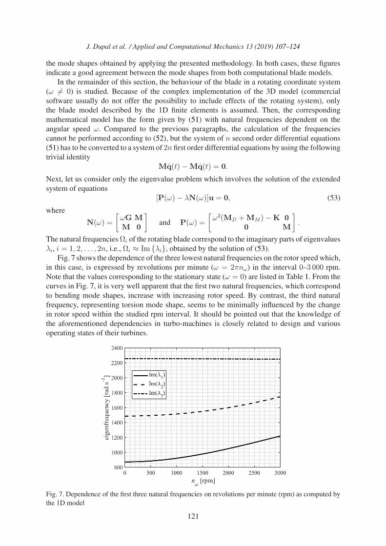
Fig. 7 shows the dependence of the three lowest natural frequencies on the rotor speed which,in this case, is expressed by revolutions per minute (ω = 2πnω) in the interval 0–3 000 rpm.Note that the values corresponding to the stationary state (ω = 0) are listed in Table 1. From thecurves in Fig. 7, it is very well apparent that the first two natural frequencies, which correspondto bending mode shapes, increase with increasing rotor speed. By contrast, the third naturalfrequency, representing torsion mode shape, seems to be minimally influenced by the changein rotor speed within the studied rpm interval. It should be pointed out that the knowledge ofthe aforementioned dependencies in turbo-machines is closely related to design and variousoperating states of their turbines.

Fig. 7. Dependence of the first three natural frequencies on revolutions per minute (rpm) as computed bythe 1D model

121


4. Conclusions

The aim of the present paper was to introduce and verify a novel 1D blade finite element with16 DOF, whose application in vibration simulations can bring a significant reduction of DOFof the total mathematical model and, at the same time, provide results that are comparable tothose obtained from 3D FE models with a much higher number of DOF. The proposed finiteelement can be implemented into any commercial software, where its connection to other typesof elements can be performed by means of transformation matrices between coupled coordinates.

Lastly, it should be pointed out that the blade finite element can serve as a starting point forvibration simulations that consider a turbo-machine as a whole, i.e., by including all the relevantparts such as shaft, generators, blade rings, bandages, bearings and sealing. In this case, oneshould realize that the total mathematical model will be periodically time-dependent becauseof stationary parts (bearings and sealing), whose stiffness and damping will vary in the rotatingcoordinate system during one revolution and be linearly dependent on the angular speed ofthe turbine. This is also the reason why the Coriolis forces are taken into consideration in thematrix of gyroscopic effects ωG. By contrast, the rotating parts of the turbo-machine (turbineshaft, generator non-symmetrical shaft, blade rings and bandages) will be time-invariable in therotating coordinate system fixed to the turbo-machine. For response determination and stabilityassessment, it is possible to use the approach and methodology described by the authors of thispaper in [2, 3, 10].

Acknowledgements

This publication was supported by the project LO1506 of the Czech Ministry of Education, Youthand Sports under the program NPU I and by the projects GA16-04546S and TE01020068.

References

[1] Chatterjee, A., Lumped parameter modelling of turbine blades packets for analysis of modalcharacteristics and identification of damage induced mistuning, Applied Mathematical Modelling40 (3) (2016) 2119–2133. https://doi.org/10.1016/j.apm.2015.09.020

[2] Dupal, J., Zajıcek, M., Analytical periodic solution and stability assessment of 1 DOF parametricsystems with time varying stiffness, Applied Mathematics and Computation 243 (2014) 138–151.https://doi.org/10.1016/j.amc.2014.05.089

[3] Dupal, J., Zajıcek, M., Analytical solution of the drive vibration with time varying parameters,Proceedings of the ASME 2011 International Design Engineering Technical Conference & Com-puters and Information In Engineering Conference IDECT/CIE 2011, Washington DC, USA, 2011.https://doi.org/10.1115/DETC2011-47830

[4] Filipov, A. P., Vibrations of mechanical systems, Naukova dumka, Kiev, 1965. (In Russian)[5] Hoffmann, T., Panning-von Scheidt, L., Wallaschek, J., Modelling friction characteristics in turbine

blade vibrations using a fourier series expansion of a real friction hysteresis, Procedia Engineering199 (2017) 669–674. https://doi.org/10.1016/j.proeng.2017.09.586

[6] Pennacchi, P., Chatterton, S., Bachschmid, N., A model to study the reduction of turbine bladevibration using the snubbing mechanism, Mechanical Systems and Signal Processing 25 (4) (2011)1260–1275. https://doi.org/10.1016/j.ymssp.2010.10.006

[7] Schwerdt, L., Hauptmann, T., Kunin, A., Seume, J. R., Wallaschek, J., Wriggers, P., Panning-VonScheidt, L., Lohnert, S., Aerodynamical and structurel analysis of operationally use turbine blades,5th International Conference on Through-Life Engineering Services 2016, Procedia CIRP Volume59, Cranfield, United Kingdom, 2016. https://doi.org/10.1016/j.procir.2016.09.023

122

https://doi.org/10.1016/j.apm.2015.09.020

https://doi.org/10.1016/j.amc.2014.05.089

https://doi.org/10.1115/DETC2011-47830

https://doi.org/10.1016/j.proeng.2017.09.586

https://doi.org/10.1016/j.ymssp.2010.10.006

https://doi.org/10.1016/j.procir.2016.09.023


[8] Segura, J. A., Castro, L., Rosales, I., Rodriguez, J. A., Urquiza, G., Rodriguez, J. M., Diagnosticand failure analysis in blades of a 300 MW steam turbine, Engineering Failure Analysis 82 (2017)631–641. https://doi.org/10.1016/j.engfailanal.2017.04.039

[9] Voldrich, J., Polach, P., Lazar, J., Mısek, T., Use of cyclic symmetry properties in vibration analysisof bladed disks with friction contacts between blades, Procedia Engineering 96 (2014) 500–509.https://doi.org/10.1016/j.proeng.2014.12.122

[10] Zajıcek, M., Dupal, J., Analytical solution of spur gear mesh using linear model, Mechanism andMachine Theory 118 (2017) 154–167. https://doi.org/10.1016/j.mechmachtheory.2017.08.008

Appendix

In this part of the work, the matrices and vector derived by applying the Lagrange’s equations inSection 2.5.1 are summarized. For better clarity of relations mentioned below, generalized matrices andvectors are defined as integrals of the product of ξ coordinate and various derivative of the function Φ(ξ)

Ikij =∫ l

0ξk ∂iΦT(ξ)

∂ξi

∂jΦ(ξ)∂ξj

dξ, iki =∫ l

0ξk ∂iΦT(ξ)

∂ξidξ. (A1)

Then, the derived matrices and vector based on the Lagrange’s equations (29) have the following forms:

• blade FE mass matrix

Me =

⎡⎢⎢⎣M11 M12 0 M14MT12 M22 0 M240 0 M33 0MT14 M

T24 0 M44

⎤⎥⎥⎦ ∈ R16,16, (A2)

where

M11 = ρS−T(3∑

i=0

ai1Ii00 + ai2Ii11

)S−1, M12 = ρS−T

(3∑

i=0

ai10Ii11

)S−1P,

M14 = −ρS−T(3∑

i=0

ai13Ii00

)S−1, M22 = ρPS−T

(3∑

i=0

ai1Ii00 + ai3Ii11

)S−1P,

M24 = ρPS−T(3∑

i=0

ai9Ii00

)S−1, M33 = ρS−T

(3∑

i=0

ai1Ii00

)S−1,

M44 = ρS−T(3∑

i=0

(ai7 + ai8)Ii00 + ai4Ii11

)S−1.

• blade FE matrix of gyroscopic effects

ωGe = ω

⎡⎢⎢⎣0 0 0 −G140 0 −G23 −G240 GT23 0 G34GT14 G

T24 −GT34 0

⎤⎥⎥⎦ ∈ R16,16, (A3)

where

G14 = 2ρS−T(3∑

i=0

ai2Ii10

)S−1, G23 = 2ρPS−T

(3∑

i=0

ai1Ii00

)S−1,

G24 = 2ρPS−T(3∑

i=0

ai10Ii10

)S−1, G34 = 2ρS−T

(3∑

i=0

ai9Ii00

)S−1.

123

https://doi.org/10.1016/j.engfailanal.2017.04.039

https://doi.org/10.1016/j.proeng.2014.12.122

https://doi.org/10.1016/j.mechmachtheory.2017.08.008


• blade FE stiffness matrix

Ke =

⎡⎢⎢⎣K11 K12 0 0KT12 K22 0 00 0 K33 00 0 0 K44

⎤⎥⎥⎦ ∈ R16,16, (A4)

where

K11 = ES−T(3∑

i=0

ai2Ii22

)S−1, K12 = ES−T

(3∑

i=0

ai10Ii22

)S−1P,

K22 = EPS−T(3∑

i=0

ai3Ii22

)S−1P, K33 = ES−T

(3∑

i=0

ai1Ii11

)S−1,

K44 = S−T(

E3∑

i=0

ai4Ii22 +G3∑

i=0

ai14Ii11

)S−1.

• blade finite element circulation matrix

KeD = −ω2Me

D = −ω2

⎡⎢⎢⎣MD11 MD

12 0 MD14

(MD12)T MD

22 0 MD24

0 0 MD33 0

(MD14)T (MD

24)T 0 MD

44

⎤⎥⎥⎦ ∈ R16,16, (A5)

where

MD11 = ρS−T

(3∑

i=0

ai2Ii11

)S−1, MD

12 = ρS−T(3∑

i=0

ai5Ii11

)S−1P,

MD14 = ρS−T

(3∑

i=0

ai13(rIi10 + Ii+110 )

)S−1, MD

22 = ρPS−T(3∑

i=0

ai1Ii00 + ai6Ii11

)S−1P,

MD24 = −ρPS−T

(3∑

i=0

ai9(rIi10 + Ii+110 − Ii00)

)S−1,

MD33 = ρS−T

(3∑

i=0

ai1Ii00

)S−1, MD

44 = ρS−T(3∑

i=0

ai15Ii00 + ai4Ii11

)S−1.

• blade FE vector of centrifugal forces

fDe =

⎡⎢⎢⎣0fD2fD3fD4

⎤⎥⎥⎦ ∈ R16,1, (A6)

where

fD2 = ρω2PS−T(3∑

i=0

ai11ii0

), fD3 = ρω2S−T

(3∑

i=0

ai1(rii0 + ii+10 )

),

fD4 = ρω2S−T(3∑

i=0

ai12ii0

).

124

Documents

1D ﬁnite element for modelling of turbine blade vibration